Non-Linear Rolling of Ships in Large Sea Wavesby

Scott M. Vanden BergB.S., Aerospace Engineering, University of Notre Dame, 1991

Submitted to the Department of Mechanical Engineering in Partial Fulfillment ofthe Requirements for the Degrees of

Master of Science in Naval Architecture and Marine Engineeringand

Master of Science in Mechanical Engineeringat the

Massachusetts Institute of Technology

11 May 2007 ~@ 2007 Scott M. Vanden Berg. All rights reserved.

The author hereby grants to MIT permission to reproduce and to distributepublicly paper and electronic copies of this thesis document in whole or in part in

any medium now known or hereafter created.

Signature ofAuthor

Department of Mechanical Engineeringx, May 11,2007

Certified by

Jerome H. Milgram, Proftssor of Mechanical EngineeringDepartment of Mechanical Engineering

Thesis SupervisorCertified by

Joel P. Harbour, Associate Professor of the Practicenpartment of Mechanical Engineering

Thesis ReaderAccepted by

Lallit Anand, Professor of Mechanical EngineeringChairman, Department Committee on Graduate Students

Department of Mechanical Engineering

MASSACHUsETTJS INSTIOF TECHNOLOGY

JUL 18 2007

LIBRARIES

Page Intentionally Left Blank

2

Non-Linear Rolling of Ships in Large Sea Wavesby

Scott M. Vanden Berg

Submitted to the Department of Mechanical Engineering on May 12, 2006 inPartial Fulfillment of the Requirements for the Degrees of

Master of Science in Ocean Engineeringand

Master of Science in Mechanical Engineering

ABSTRACT

The United States Navy has taken a new interest in tumblehome hulls.

While the stealth characteristics of these hull forms make them attractive to the

Navy, their sea keeping characteristics have proven to be problematic. Normal

approximations of sea keeping characteristics using linear differential equations

with constant coefficients predict a very stable platform, while observations in

model tests show a ship that is prone to extreme roll transients. This thesis

examines a simple method of producing a non-linear simulation of roll motion

using a tumblehome hull provided by the Office of Naval Research. This

research demonstrates the significant difference that a variable restoring

coefficient introduces into a hull's seakeeping characteristics.

Thesis Advisor: Jerome H. MilgramTitle: Professor of Mechanical Engineering

Thesis Reader: Joel P. HarbourTitle: Associate Professor of the Practice

3

Acknowledgements

The author would like to acknowledge the following organizations and individualsfor their assistance. Without them this thesis would not have been possible.

. Professor Yuming Liu, for his aid in computer simulation schemes

* LT Andrew Gillespy (USN), and LT(jg) Kyriakos Avgouleas, who werefantastic sounding boards during my research

* CDR Joe Harbour for advisement as thesis readers

. Mr. William Belknap from Naval Surface Warfare Center, Carderock Division,for the use of the ONR tumblehome hull form

. Finally, Professor Jerry Milgram, for his advice and experience

4

Table of Contents

ABSTRACT ...................................................................................................... 3Acknowledgem ents ......................................................................................... 4Table of Contents .............................................................................................. 5List of Figures .................................................................................................. 6List of Tables .................................................................................................... 71 Introduction ............................................................................................... 9

1.1 M otivation for Research ..................................................................... 91.2 O bjective and Outline of Thesis ........................................................ 9

2 The O NR Tum blehome Hull ................................................................... 112.1 Hull Description ................................................................................. 112.2 Com puter M odeling in Maxsurf and M atlab....................................... 132.3 Non-Linearities in Righting Moment .................................................. 152.4 Seakeeping Scenario ........................................................................ 16

3 Linear Seakeeping Theory ..................................................................... 173.1 Linear Plane Progressive W aves ...................................................... 173.2 W ave Spectra.................................................................................... 193.3 Equations of Motion & Linear Superposition .................................... 223.4 Treatm ent of Roll in MAXSURF ........................................................ 27

4 Roll Excitation M oment............................................................................. 304.1 Froude-Krylov Moment...................................................................... 304.2 Diffraction M om ent .......................................................................... 32

4.2.1 Diffraction Boundary Value Problem ......................................... 324.2.2 Num erical Determ ination of Diffraction Potential........................ 33

5 M atlab Code Description .......................................................................... 345.1 Files Required from Maxsurf ............................................................. 355.2 Excitation Force Calculator ............................................................... 375.3 Linear Response Generator............................................................. 405.4 Non-Linear Response Generator .................................................... 41

6 Sim ulation Results.................................................................................... 436.1 Sea Keeper and Linear Integration Sim ulations................................ 436.2 Linear Integration and Non-Linear Integration................................... 45

7 Future W ork and Conclusion.................................................................... 487.1 Added M ass and Dam ping ............................................................... 487.2 Directional Seas ............................................................................... 497.3 Non-linear Excitation Mom ents ........................................................ 497.4 W ave Profile Effects on Righting M om ent......................................... 497.5 Conclusion ....................................................................................... 49

List of References............................................................................................ 51Appendix A: M atlab Code for Finding Excitation Forces................................. 52Appendix B: List of Sym bols.......................................................................... 66

5

List of Figures

Figure 2-1: Profile View of the ONR Tumblehome Hull. ................................. 11Figure 2-2: Body Plan of ONR Tumblehome Hull........................................... 12Figure 2-3: Righting Arm Curves for Different Hull Shapes ............................. 13Figure 2-4: Righting Moment vs. Trim for Roll=1 0, Draft=5.5m ....................... 15Figure 2-5: Righting Moment vs. Draft, Roll=10, No pitch ............................... 16Figure 2-6: Seakeeping Scenario................................................................... 17Figure 3-1: Fully Developed Bretschneider (Pierson-Moskowitz) Spectrum for

S ea S tate E ig ht ...................................................................................... . 20Figure 3-2: Simulated Wave Elevation Record for Sea State Eight................. 22Figure 3-3: Heave Response in Sea State Eight Time Simulation from Sea

K e e p e r.................................................................................................... . 2 6Figure 3-4: Pitch Response in Sea State Eight Time Simulation from Sea Keeper

................ .......... ..... ........... ... . ..... ...... ....................... . ........ 2 7Figure 3-5: Roll Response Time Simulation from Sea Keeper ........................ 30Figure 4-1: Normal Vector for Moments ........................................................ 31Figure 4-2: Domain for Diffraction Boundary Value Problem.......................... 34Figure 5-1: ForceFinder Block Diagram........................................................... 37Figure 5-2: findfk Block Diagram ................................................................... 38Figure 5-3: Excitation Moments for Seakeeping Problem................................ 39Figure 5-4: Block Diagram for Non-Linear Roll Integration............................. 42Figure 6-1: Modulus of Non-dimensional Excitation Force vs. Frequency..... 43Figure 6-2: Roll Angle vs Time from Linear Integration and Response Spectrum

........ .......... ...... .... ... ....... . . . ....... ............................. .... ... . . . .... .. 4 5Figure 6-3: Linear Simulation vs. Non-linear Simulation with Larger Rolls in the

L ine a r C a se ............................................................................................. . 4 6Figure 6-4:Linear Simulation vs. Non-linear Simulation with Larger Rolls in the

N o n-linea r C ase ...................................................................................... . 47

6

List of Tables

Table 5-1: Righting Moment vs. Roll, Pitch, & Draft ...................................... 36Table 6-1:Comparison of Different Roll Response Calculations...................... 48

7

Page Intentionally Left Blank

8

1 Introduction

1.1 Motivation for Research

Naval architecture in the United States Navy has come full circle. With the

selection of a tumblehome hull for the DDG-1 000 project, the United States Navy

has come back to a design concept that was used on the oldest commissioned

warship in their fleet, the USS Constitution. Tumblehome, the inward slope of

the upper part of the hull of a ship, has come back in style due to the stealthy

benefits it imparts upon its ship. However, with the use of this 'new' concept

come interesting challenges in naval architecture.

The latest designs for the hulls of United States naval warships have

sparked a controversy over their stability. In the April 2007 edition of the Navy

Times, experts are quoted stating that the hull may be unstable in roll motion.[1]

Programs that use linear sea keeping approximations predict good stability for

tumblehome hulls. However, non-linear effects in the coupling of pitch and

heave with roll motions can degrade the stability of a tumblehome ship.

Programs that calculate the non-linear effects of this nature may require

significant computing power making them costly and time consuming. A simpler

approach could reduce computing requirements and allow naval architects to

quickly estimate the stability of any new hull.

1.2 Objective and Outline of Thesis

The purpose of this thesis is to explore the non-linear effects that pitch,

heave, and roll exert on a ship's restoring moment. The linear seakeeping

equations will be modified to allow the restoration force to be calculated as a

function of roll, pitch, and heave. Time simulations of pitch and heave responses

derived from linear seakeeping theory are used to provide a basis for numerical

solution of the non-linear seakeeping equation for roll. Although the research

presented is for one specific hull form and operating condition, the methods used

are intended to applicable to any ship in any seakeeping situation. Chapter Two

discusses the characteristics of the hull used in this research, including the

9

operational scenario that is used for conducting the research. Chapter Three

explains linear seakeeping theory, as well as the approximations used by the

seakeeping program Maxsurf. Chapter Four discusses the method used to

determine the excitation forces used in the non-linear simulation. Chapter Five

describes the computer programs used to simulate the roll motion of the ship.

Chapter Six presents a comparison of the linear and non-linear results, and

Chapter Seven presents recommendations for future work and conclusions.

10

2 The ONR Tumblehome Hull

2.1 Hull Description

The hull form used for this thesis is the tumblehome hull used by the

Office of Naval Research. This ship has a length of 154 meters and a beam of

18.5 meters. The displacement at a draft of 5.5 meters is approximately 8800

metric tons.[2] The hull has a vertical center of gravity assumed to be 7.5 meters

above baseline, and the transverse metacentric height is 1.47 meters. The bow

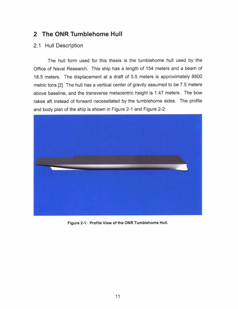
rakes aft instead of forward necessitated by the tumblehome sides. The profile

and body plan of the ship is shown in Figure 2-1 and Figure 2-2:

Figure 2-1: Profile View of the ONR Tumblehome Hull.

11

Figure 2-2: Body Plan of ONR Tumblehome Hull

The tumblehome hull has military advantages that make it attractive for

use in surface combatants. The chief advantage comes from the fact that the

sides of the hull are angled away from the waterline. This will tend to reflect

radar energy that is directed towards the ship from another up into the

atmosphere, and not back towards the radar receiver. This scattering of radar

energy significantly reduces the radar cross section of the ship, making the ship

harder to detect.

From a naval architecture standpoint, tumblehome hulls have some less

than ideal properties. The decreasing beam above the waterline limits the

deckhouse area, and reduces the damaged stability of the hull form compared to

wall sided or flared hulls. In the area of stability, the hull suffers compared to

traditional hull forms. As the ship lists, the tumblehome causes a relative

reduction in the waterplane area of the ship, lowering the righting arm. The

righting arm for zero pitch is shown in Figure 2-3, compared to ships with similar

shapes, but with wall sides and flare instead of tumblehome.

12

- - - -- ----- ------- --------- ------- ----- -----

1.4

1.2

0.3

0.1

0.4

0.2

-0.2-

Medium GM (1.5m) Righting Arm Curves

-- Tumblehome(SHCP)--- Wall-Sided (SHCP)

-- Flare-Sided (SH CP)

1 2C 30 40 ( ec d r, 8 s)

-Heel Angle(degrees)

Figure 2-3: Righting Arm Curves for Different Hull Shapes

The wave piercing bow has its own military advantages. Because of the

reduced buoyancy of the bow, the ship tends to pitch less as it rides through

waves, giving the ship a more stable platform for its weapons systems.

Additionally, the design may reduce the waves generated by the ship, lowering

resistance of the hull. These advantages come at a price in the stability analysis.

The ship loses waterplane area as it pitches down by the bow, resulting in a

smaller transverse righting arm as the bow sinks into the water. In most

operating cases, this effect can be neglected. In heavier seas where pitch is

significant, the loss of righting arm can cause severe rolling transients.

2.2 Computer Modeling in Maxsurf and Matlab

The ONR tumblehome hull was provided by the Carderock Division of the

Naval Surface Warfare Center. In order to conduct this research, it was modeled

in both Maxsurf and Matlab. Offsets were generated in Maxsurf using a

computer aided drawing of the hull. The offsets were used in three different parts

of this research.

First, Maxsurf's Sea Keeper module used the offsets to determine a pitch,

heave, and roll response using the program's linear strip theory calculations.

These outputs were in the form of linear response amplitude operators (RAOs)

13

----------- ............

for both magnitude and phase relative to the incident waves. As explained in

Chapter Five, the RAOs were used to generate a time simulation of the ship's

pitch, heave, and roll. The pitch and heave time simulations were used to

determine the non-linear roll righting moment. The roll response was used to

compare against the results of the non-linear simulation. The offsets were also

used to model the ship in Matlab to determine excitation forces. The offsets were

used as a set of nodes to compute the Froude-Krylov and diffraction excitation

moments. Finally, the hull offsets were used in Maxsurf's Hydromax module to

determine the ship's righting moment in roll as a function of pitch, heave, and roll.

This will be explained in Section 2.3.

Mass distribution for the ship was chosen to approximate a ship with a

relatively high center of gravity to allow for high weight, such as weapons

systems on a naval vessel. The center of gravity was chosen to be on the

centerline two meters above the still waterline. This was arbitrarily chosen so

that the metacentric height would match the height shown in Figure 2-3. The

longitudinal position was determined as directly above the center of buoyancy to

give the ship no trim in pitch. In order to match Maxsurf approximations, an

estimate of 40 percent of the ship's beam was used to approximate the ship's

radius of gyration. Therefore the roll moment of inertia is given by the formula:

,44 = (0.4B) 2 pV (2.1)

This mass distribution may be used to estimate the undamped natural

period of the hull [5] through the use of the equation

T = 27c ( + A 4 ) (2.2)pVgGM,

The added mass in roll, A44 , was assumed to be 0.3 times the mass

moment of inertia, as discussed in Section 3.4. For the values given in this

section, the natural period is approximately 13.9 seconds. This will be used to

compare against results in Chapter Six.

14

2.3 Non-Linearities in Righting Moment

One of the unique aspects of a tumblehome hull is its roll restoring

moment behavior with its movement in the three principal degrees of freedom.

Because of the wave piercing bow, its buoyancy forward is much smaller than its

buoyancy aft. This asymmetry leads to a non-linear behavior in restoring

moment. As mentioned in the previous section, the offsets were used to

determine the hydrostatic righting moment as a function of roll angle, pitch angle,

and draft.

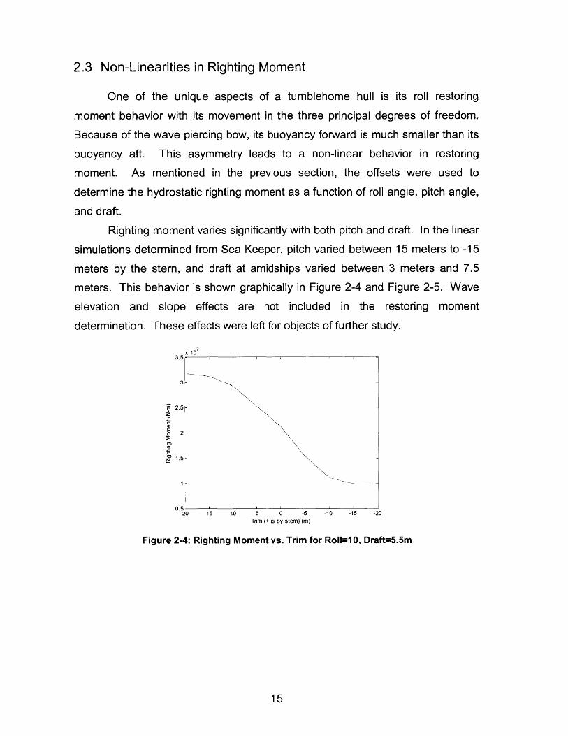
Righting moment varies significantly with both pitch and draft. In the linear

simulations determined from Sea Keeper, pitch varied between 15 meters to -15

meters by the stern, and draft at amidships varied between 3 meters and 7.5

meters. This behavior is shown graphically in Figure 2-4 and Figure 2-5. Wave

elevation and slope effects are not included in the restoring moment

determination. These effects were left for objects of further study.

x 10

3-

E2 2.5-

:E

-9 1.5-

1- - -

0.520 15 10 5 0 -5 -10 -15 -20

Trim (+ is by stem) (m)

Figure 2-4: Righting Moment vs. Trim for RoIl=10, Draft=5.5m

15

2.3 Non-Linearities in Righting Moment

One of the unique aspects of a tumblehome hull is its roll restoring

moment behavior with its movement in the three principal degrees of freedom.

Because of the wave piercing bow, its buoyancy forward is much smaller than its

buoyancy aft. This asymmetry leads to a non-linear behavior in restoring

moment. As mentioned in the previous section, the offsets were used to

determine the hydrostatic righting moment as a function of roll angle, pitch angle,

and draft.

Righting moment varies significantly with both pitch and draft. In the linear

simulations determined from Sea Keeper, pitch varied between 15 meters to -15

meters by the stern, and draft at amidships varied between 3 meters and 7.5

meters. This behavior is shown graphically in Figure 2-4 and Figure 2-5. Wave

elevation and slope effects are not included in the restoring moment

determination. These effects were left for objects of further study.

X 1073.5: 1

3

2.5-

0 22

1.5-

1-

0.5120 15 10 5 0 -5 -10 -15 -20

Trim (+ is by stem) (m)

Figure 2-4: Righting Moment vs. Trim for RoIl=10, Draft=5.5m

15

.............. ... ...... ..... .... .... .........

U=12.8m/s

x

y

A,w

1=rr/3

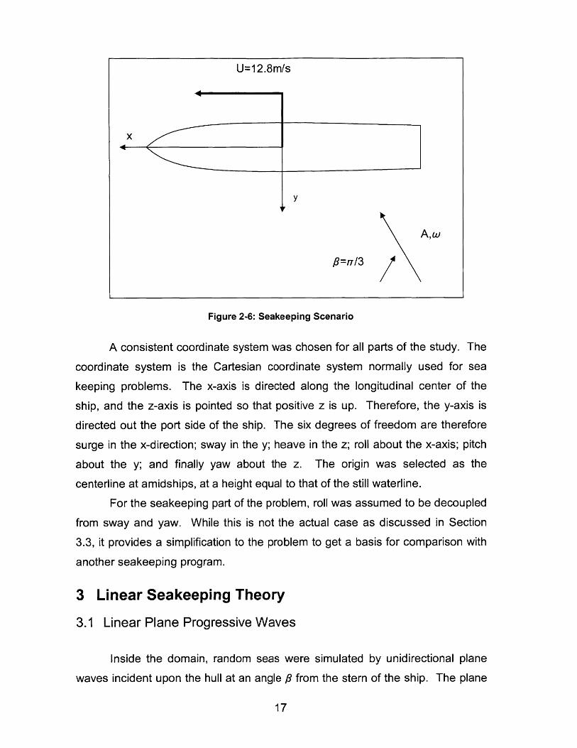
Figure 2-6: Seakeeping Scenario

A consistent coordinate system was chosen for all parts of the study. The

coordinate system is the Cartesian coordinate system normally used for sea

keeping problems. The x-axis is directed along the longitudinal center of the

ship, and the z-axis is pointed so that positive z is up. Therefore, the y-axis is

directed out the port side of the ship. The six degrees of freedom are therefore

surge in the x-direction; sway in the y; heave in the z; roll about the x-axis; pitch

about the y; and finally yaw about the z. The origin was selected as the

centerline at amidships, at a height equal to that of the still waterline.

For the seakeeping part of the problem, roll was assumed to be decoupled

from sway and yaw. While this is not the actual case as discussed in Section

3.3, it provides a simplification to the problem to get a basis for comparison with

another seakeeping program.

3 Linear Seakeeping Theory

3.1 Linear Plane Progressive Waves

Inside the domain, random seas were simulated by unidirectional plane

waves incident upon the hull at an angle fl from the stern of the ship. The plane

17

waves were assumed to be a superposition of sinusoidal waves at different

frequencies. To treat the waves using potential theory, the following

assumptions were made. First, the unsteady viscous forces on the hull are

neglected. Next, the density of the seawater is constant and all flows were

incompressible. Finally flow was approximated as being irrotational.

All flow potential functions must satisfy conservation of mass. With the

assumption of incompressible flow, the conservation of mass states that the

divergence of the velocity field must be zero. In mathematical terms, this means

that the governing equation for all potentials must be:

au' aW' a 2 a24-- + - =_+_ = V2(1 = 0 (3.1)ax' aZ' ax' 2 az' 2

In equation(3.1), the primed quantities are with respect to a coordinate

system with the waves propagating in the x' direction. The two boundary

conditions for these come from the kinematics of the waves and the dynamic

pressure of the wave's surface. The kinematic boundary condition is that along

the wave surface, z=4 where ; (x,y,t) is the wave elevation as a function of

position and time. By defining a function F=z- , then the kinematic boundary

condition may be written as:

DF OF( FS= -t +(V.V)F = on z- =(3.2)

Dt at+ ) Ol=

The dynamic free surface condition comes from the fact that the

pressure is atmospheric along the surface of the wave. From Bernoulli's

equation for potential flow,

a0 1P-- +- V-VD+ gz = - on z= (3.3)at 2 p

In most case, the wave slopes encountered are small, so these

equations may be treated by linearizing the boundary conditions. The linearized

boundary conditions become:

a+2 g - & -- on z=0 (3.4)at az g at

18

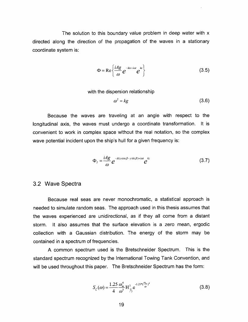
The solution to this boundary value problem in deep water with x

directed along the direction of the propagation of the waves in a stationary

coordinate system is:

D= Re {' e ix+iot"e (3.5)

with the dispersion relationship

C = kg (3.6)

Because the waves are traveling at an angle with respect to the

longitudinal axis, the waves must undergo a coordinate transformation. It is

convenient to work in complex space without the real notation, so the complex

wave potential incident upon the ship's hull for a given frequency is:

~, iAg -ik(xcos/3-ysin /3)+iwt kz (7e e(37

3.2 Wave Spectra

Because real seas are never monochromatic, a statistical approach is

needed to simulate random seas. The approach used in this thesis assumes that

the waves experienced are unidirectional, as if they all come from a distant

storm. It also assumes that the surface elevation is a zero mean, ergodic

collection with a Gaussian distribution. The energy of the storm may be

contained in a spectrum of frequencies.

A common spectrum used is the Bretschneider Spectrum. This is the

standard spectrum recognized by the International Towing Tank Convention, and

will be used throughout this paper. The Bretschneider Spectrum has the form:

1.25 W,4 -(3.8)Sg~ ~~ ()) = - H 3 ' 3

19

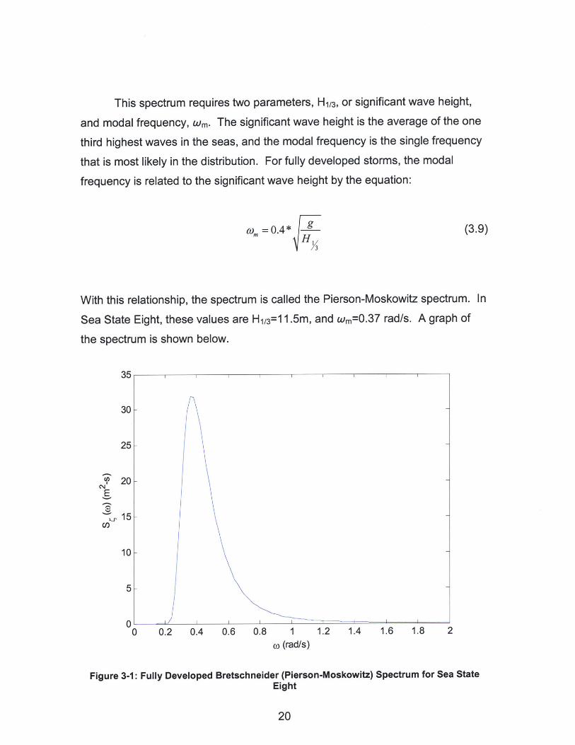
This spectrum requires two parameters, H1/3, or significant wave height,

and modal frequency, wm. The significant wave height is the average of the one

third highest waves in the seas, and the modal frequency is the single frequency

that is most likely in the distribution. For fully developed storms, the modal

frequency is related to the significant wave height by the equation:

(3.9)co. = 0.4* gH1

3

With this relationship, the spectrum is called the Pierson-Moskowitz spectrum. In

Sea State Eight, these values are H1/3=1 1.5m, and wm=0.3 7 rad/s. A graph of

the spectrum is shown below.

C/)

35

30-

25-

20-

10-

0 0.2 0.4 0.6 0.8 1t) (rad/s)

1.2 1.4 1.6 1.8 2

Figure 3-1: Fully Developed Bretschneider (Pierson-Moskowitz)Eight

Spectrum for Sea State

20

I I I I I

5

n

. .. .. .. .... . .. .........

When scaled by pg, the area under the spectrum curve represents

the energy per unit area of the sea state. Because of the assumption that the

sea state is described by a collection of waves at distinct frequencies, this energy

relationship can be used to simulate a random sea state in a discrete form. For a

random sea, the energy density of the system may be expressed as

#freqsA 2 00

E = pg = Pg JS(w)do (3.10)

By discretizing the integral in the above relationship, the wave

amplitudes for discrete frequencies, separated by A o, can be calculated as:

A = 2S (CO)Ao) (3.11)

Adding in a random phase angle, random seas may be simulated

on a computer rather quickly using only the formula for the wave height

spectrum. The surface elevation on a fixed (x,y) vertical line (t) is simply

#freq

it =s(Ot + (3.12)

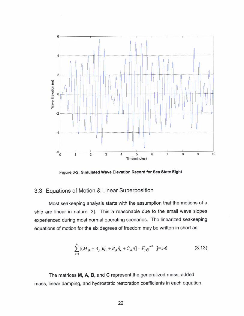
An example of the record of a random sea in Sea State Eight is shown in

figure 3-2. The sea state was generated using 500 discrete frequencies equally

spaced from 0 to 2.5 radian/second, calculated every .01 seconds.

21

III I I I I I

- I0 1 2 3 4 5

Time(minutes)6 7 8 9 10

Figure 3-2: Simulated Wave Elevation Record for Sea State Eight

3.3 Equations of Motion & Linear Superposition

Most seakeeping analysis starts with the assumption that the motions of a

ship are linear in nature [3]. This a reasonable due to the small wave slopes

experienced during most normal operating scenarios. The linearized seakeeping

equations of motion for the six degrees of freedom may be written in short as

6 io.)t J = 6

L [(Mjk ± Ajk )k +Bjkl k ±Cjk?]= Fe j=6k=1

(3.13)

The matrices M, A, B, and C represent the generalized mass, added

mass, linear damping, and hydrostatic restoration coefficients in each equation.

22

C0

0

-2

-4

I I I I I I ~ I I I

. . ......... -- ---------

----------------------- ---- --- --- -------------------

------- --- --- --- --------- -------- --------

----------- -- ----- ---- --- -------- --------- L

I--------------- --------------- -------------------------

-- --- --- -------------- ----------------------------- -------------

-- -------- -------- ---- --- -- --- ------ ----------- -- -------

----- -----

---------- ------ --- --- -----

------- ---------------------------------------------------- -

Because of the lateral symmetry of the ship, several terms can be set to zero.

The result is that the generalized mass matrix has the form:

0

m

0

-mzC

0

0

0

0

m

0

0

0

0

-mz

0

144

0

-146

mz

0

0

0

155

0

0

0

0

-146

0

166

The added mass matrix has the form:

0 A 13

A 2 2 0

0 A 33

A 4 2 0

0 A53

A62 0

0 A 15 0

A 24 0 A 26

0 A35 0

A 44 0 A 46

0 A55 0

A64 0 A66

The damping coefficient matrix

matrix. The damping coefficients

has the same

are non-zero

shape as the added mass

where the added mass

coefficients are non-zero, and zero everywhere else.

Almost all of the restoring coefficients for ships on the ocean surface are

zero. The only non-zero terms are C33, C44, C55, C35, and C53. Expanding the

equations with all coefficients in them shows a very interesting phenomenon.

Because of the symmetrical zeroes in each matrix, the whole system divides into

two sets of three coupled equations; one set consisting of surge, heave, and

pitch, and the other set describing sway, roll, and yaw. This can further be

simplified, as Salveson, et.al point out[4], by noting that the surge force and the

surge response, are very small compared to the other forces and motions. The

equations of motion for each fixed frequency are then:

23

m

0

0

0

mz

0

A11

0

A 3 1

0

A5 1

0

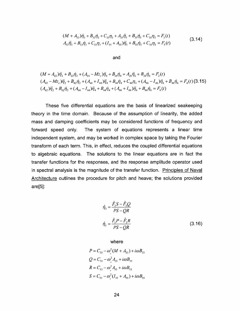
(M + A33)ij +B 3343 + C3373+ AA +B3A5 + C35 175 = F3(t)

A5A +B33 + C5317 3 + (15 +A55 )kj + B5A5 + C5575 = F,(t)

and

(M + A222 A+B 2A + (A2 -Mzc)i 4 +B +A 26A +B2 6 =F2 (t)

(A42 -Mz c)ij 2 +B 42t + (A 4 4 +144) 74 ±B 4 ±C44 774 +(A46 -I46 ) k+B 4 NA = F4(t) (3.15)

(A 62 )42 + B 62 2 + (A64 - 64 )4 + B 6 + (A66 + I66) A +B = FW (

These five differential equations are the basis of linearized seakeeping

theory in the time domain. Because of the assumption of linearity, the added

mass and damping coefficients may be considered functions of frequency and

forward speed only. The system of equations represents a linear time

independent system, and may be worked in complex space by taking the Fourier

transform of each term. This, in effect, reduces the coupled differential equations

to algebraic equations. The solutions to the linear equations are in fact the

transfer functions for the responses, and the response amplitude operator used

in spectral analysis is the magnitude of the transfer function. Principles of Naval

Architecture outlines the procedure for pitch and heave; the solutions provided

are[5]:

FS - FQ773 - 3S 5

PS -QRAA

FP-FR75 = FP FR (3.16)

PS - QR

where

P=C -w)(M+ A3 3 ) +ioB 33

Q = C 35 -Oe35 +iCoB 35

R _= C 3 - A+ +iwB5 3

s=c 55 -C 2 (155 + A 5 )+iB 55

24

It should be noted that the transfer functions are complex operators, with

only the real part of the product having physical meaning. An equivalent

expression which is used in Maxsurf and later in the computer programming is

the modulus and phase of the transfer function H(co), as shown below:

H() - = H(co) e"ia() (3.17)A

However, the transfer functions are only one third of the picture. The

other two parts are the hydrodynamic coefficients in the equations and the

excitation forces. These values are difficult to compute, and that difficulty is

compounded by the fact that many of the coefficients depend on the frequency of

the incident waves. Additionally, the excitation forces depend on both the

frequency and amplitude of the incident waves. The amplitude of the waves is

treated by non-dimensionalizing the response. Forces and displacements are

considered proportional to the amplitude of the wave, so the non-dimensional

response is q /A and the excitation for is per unit amplitude. Likewise, the non-

dimensional angular displacements are 7 / kA.

As mentioned, the added mass and damping coefficients are dependent

on both the frequency and forward speed of the ship in a seakeeping scenario.

This thesis treats the added inertia and damping coefficients for roll as constants.

This simplifies calculations and provides a basis for comparison with the results

for Maxsurf.

For pitch and heave motion, the Sea Keeper module of Maxsurf was used

to obtain both the hydrodynamic coefficients and the exciting forces. The

resultant transfer functions and the discretized wave spectrumwere transformed

into time series for both pitch and heave. The wave heights and phases at many

discrete frequencies were determined as discussed in section 3.3. The response

at time t becomes:

#fteq

7 ) W A,,,RAO(o),,, )cos(ot +/,,,) (3.18)M=1

25

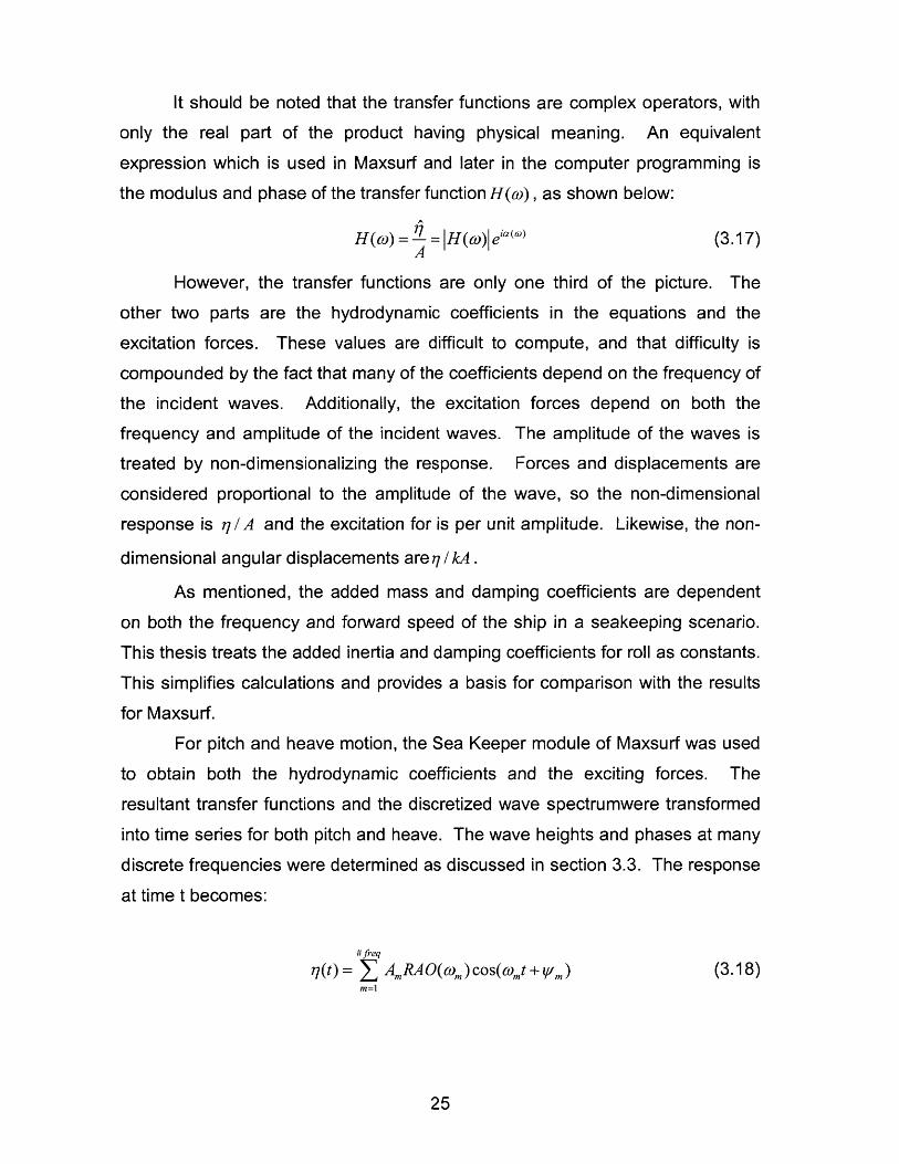
Examples of the pitch response and heave response of the ONR

tumblehome hull are shown in the figures below. The pitch and heave responses

were used as inputs to the righting arm function discussed in section 5.4.

E)

(DCU

6

4

2

0

-2

-4

6r0 1 2 3 4 5 E

Time (minutes)7 8 9

Figure 3-3: Heave Response in Sea State Eight Time Simulation from Sea Keeper

26

-------------- ------------ -- -- -- ---- -- - ------ --- -- - --------

-- -- -- -- - --------- - -- - -- - --- ---- -- ---- -

------------ ---

------------------------------------------------------------------

10

. ... ....... ...

15 I I I I I I

1E 5 -- - - --- --- --- - ----- --- --- --- -- - - ------- - - --------- -- --- -- -

- 0-- ----------

-5 ----- -- - - ---- --- ---- - ---------- - --------- -- ---

-150 1 2 3 4 5 6 7 8 9 10

Time (minutes)

Figure 3-4: Pitch Response in Sea State Eight Time Simulation from Sea Keeper

The mean period for pitch is 17.3 seconds, with a root mean square

average amplitude of 1.9 degrees. This translates to ±5.2 meters of pitch over

the length of the ship. The heave period is 21 seconds, with an average

amplitude of 2.4 meters.

3.4 Treatment of Roll in MAXSURF

Maxsurf uses the same linear sea keeping equations as described in

Section 3.3 with three important differences.[4] First, roll is assumed to be

uncoupled from sway and yaw. In other words, the roll degree of freedom is

simulated as its own independent mass-spring-dashpot system. The reasoning

for decoupling roll from sway and yaw is due to the large force and moment that

the rudder places on a ship. Since this is often ignored in seakeeping, the

relatively smaller wave force and moment are ignored. The roll equation with this

assumption becomes

27

-- - I - - - - ... .... .... , - ... .... .......

(144 + A )ij +B4 + C4r7 = F4e( 3.

The second assumption that Maxsurf makes deals with the added mass

and damping coefficients. In normal seakeeping theory, these coefficients are

functions of excitation frequency and forward speed. This requires calculations

in the frequency domain with an inverse Fourier transform (IFFT) to obtain a time

domain solution. For Sea Keeper, they are assumed to be constants. The

equation is then an ordinary linear differential equation in the time domain with

constant coefficients, with the solution

Fr74 4 cos(t + a) (3.20)

V(C 44 -(44 +A 44 )w )2 +)BCoe

tan(a) = B44 C (3.21)C44 -(U44 +A4 )(C3.

The mass moment of inertia is calculated with a user-defined roll gyradius,

as described in equation (2.1) . The added mass is set to 0.3 times the moment

of inertia of the ship, and the damping coefficient is set by the user through the

input of a damping ratio, 844. For this research, the Maxsurf default value of

0.075 was used for all calculations. The damping coefficient is calculated

according to the equation

B44 = 2,44 C44(144 + A44) (3.22)

Normally, the damping ratio is a function of frequency, making the

equation true for each frequency separately. However, the frequency

dependence is neglected by making 844 a constant. This permits a direct time

domain solution.

28

(3.19 )

Finally, Sea Keeper does not calculate the excitation moment using a

rigorous method. It assumes that the moment may be approximated as the

product of the wave slope and the hydrostatic righting moment, in phase with the

wave slope. Therefore:

F4 =kAC44

where

C44 = pgVGM,

(3.23)

(3.24)

Using all of the values from this section, the roll response amplitude

operator for roll becomes

_L = RAOkA

CC44

j(C4 - (144 ±A44) W2) 2 + CoeB 44

The roll response amplitude operator may be used in conjunction with the

wave height spectrum to produce a time series simulation just as in pitch and

heave. An example of the time simulation for roll is shown below:

0 1 2 3 4 5 6Time (minutes)

7 8 9 10

29

(3.25)

30

20

10

0

-10

-20

1

CD

'a

C

----- --- -

---- -- -- -- -

-.. ...... - ---- --- - ---

---- --- --- -------

. . .... ..... .... .. ......... .... ... .... ... ..... .....

I I

-----------------

-- -- ------

-----------------

-4 ------- ---- - --

-

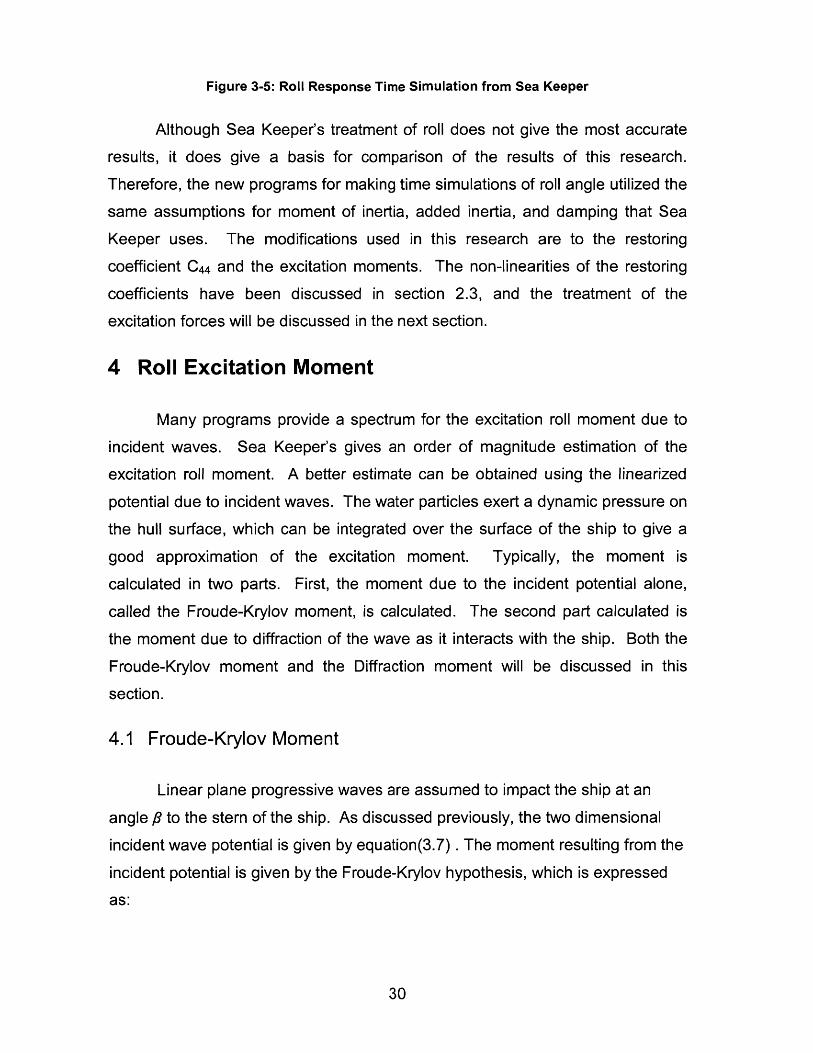
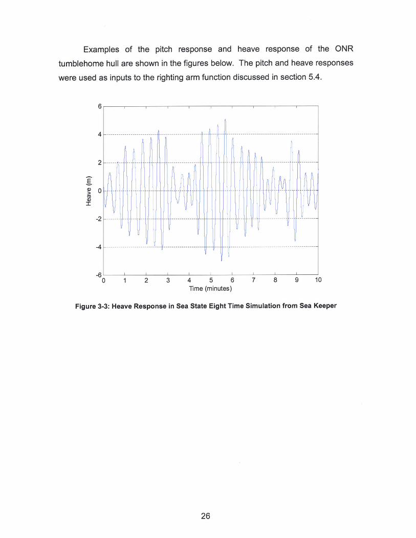
Figure 3-5: Roll Response Time Simulation from Sea Keeper

Although Sea Keeper's treatment of roll does not give the most accurate

results, it does give a basis for comparison of the results of this research.

Therefore, the new programs for making time simulations of roll angle utilized the

same assumptions for moment of inertia, added inertia, and damping that Sea

Keeper uses. The modifications used in this research are to the restoring

coefficient C44 and the excitation moments. The non-linearities of the restoring

coefficients have been discussed in section 2.3, and the treatment of the

excitation forces will be discussed in the next section.

4 Roll Excitation Moment

Many programs provide a spectrum for the excitation roll moment due to

incident waves. Sea Keeper's gives an order of magnitude estimation of the

excitation roll moment. A better estimate can be obtained using the linearized

potential due to incident waves. The water particles exert a dynamic pressure on

the hull surface, which can be integrated over the surface of the ship to give a

good approximation of the excitation moment. Typically, the moment is

calculated in two parts. First, the moment due to the incident potential alone,

called the Froude-Krylov moment, is calculated. The second part calculated is

the moment due to diffraction of the wave as it interacts with the ship. Both the

Froude-Krylov moment and the Diffraction moment will be discussed in this

section.

4.1 Froude-Krylov Moment

Linear plane progressive waves are assumed to impact the ship at an

angle fl to the stern of the ship. As discussed previously, the two dimensional

incident wave potential is given by equation(3.7) . The moment resulting from the

incident potential is given by the Froude-Krylov hypothesis, which is expressed

as:

30

(4.1)M2K = pfD n4 dSC

In complex space, the Froude-Krylov hypothesis is written:

(4.2)M4 F'K =icp J 1 n4dSC

In this case, the surface C is the wetted surface of the ship's hull in still

water, and the normal vector component, n4 , is the cross product of the hull's

two-dimensional normal vector with the position vector of the point in question,

shown in Figure 4-1:

n

n4 = Ir X n I

Figure 4-1: Normal Vector for Moments

The method of numerical analysis becomes quite clear. For a given

section, the normal and incident potential are known at each point in the table of

offsets. The complex sectional Froude-Krylov force is expressed as:

#points #points

f4FK =I yn9 En 4,n =pAg I e (4.3)n=1 n=1

And the overall moment can be calculated using a trapezoidal rule along thelength of the ship:

31

j

(4.4)FFK #stations-1 (f4,m + f4,m+1)

2 (X. - XM+i)Fn=t 2

4.2 Diffraction Moment

The excitation moment

the ship is more complicated.

moment used by Milgram [6].

moment may calculated as

due to the diffraction of waves around the hull of

This thesis uses the calculation of the diffraction

Like the Froude-Krylov moment, the diffraction

M = -)PfJ ndSC

(4.5)

The problem is that the diffraction potential is not known, and more than

likely can not be found as an explicit function of position and time. Therefore,

numerical methods must be used to determine the diffraction potential before

numerical integration can be implemented.

4.2.1 Diffraction Boundary Value Problem

Just as in the case of plane progressive waves, the diffraction potential

must satisfy a fluid flow boundary value problem. The boundary value problem

can be stated as follows: the total potential must satisfy mass conservation

inside the fluid, with no flux along the hull of the ship or bottom boundary of the

domain. The potential of the sides and free surface reflect the fact that the

diffraction will produce waves radiating outward. Therefore, the diffraction

potential satisfies the following equations:

V2#D = 0

a8bD a8 i =0L9D+ 0an an

D = 0az

-o D D = 0an

(4.6)

(4.7)

(4.8)

(4.9)

(Field Condition)

(On the Hull)

(Bottom)

(Free Surface)

32

&5D = -ikD (4.10) (On the Sides)an

4.2.2 Numerical Determination of Diffraction Potential

Once the boundary conditions are known, the potential may be

determined using a constant panel method using Green's theorem. The methd

for determining the diffraction potential is modeled on that used by Milgram[6]. It

is known that the potential obeys Laplace's equation in the field. Another

function that satisfies LaPlace is required for Green's theorem. In this case, the

Rankine Green's function was used. The Rankine Green's function takes the

form

G(y, z, ,g)=-ln(V(y -)) 2 + (z - (4.11)

This function therefore depends on the distance from the field point (y,z)

and the source point (r7,g). Because both the diffraction potential and Green's

function satisfy LaPlace's equation, Green's theorem states that the following

equation is true along the boundary of the domain:

4((D G -G 'D)ds = -7(y, z) (4.12)s an (q,g ) an(77,g)

To solve this numerically, the domain must be divided into several panel

line elements. Along each panel, the values of 0 and 650/t5n in the equation

above may be assumed to be constant. This means that the panels must be

small enough that the potential does not change significantly across the panel.

This becomes important is selecting the domain size, since more panels

significantly increases the computation time for each section. The result

becomes a summation throughout the domain, namely:

L n de .+r .O6 = 1n1 G.dt? (4.13)1 JL1 an1 j =1 franl., UI

33

The integrals in the above equation can be computed numerically as well.

The boundary conditions provide relationships to eliminate the derivative of the

diffraction potential at each point. This reduces the system to a set of N linear

equations for the diffraction potential.

For the problem, a two dimensional domain chosen for this problem is a

box of ocean fluid with the hull in the center of the top, as shown in Figure 4-2:

H

B

W

Figure 4-2: Domain for Diffraction Boundary Value Problem

The half-width of the domain W was set to ten ship beams. This width

was determined to be acceptable for convergence by Milgram [6]. The depth H

was set to one half the wavelength of the incident wave or three times the draft T,

whichever was greater. This brings the domain to where the incident potential is

near zero for long waves, and covers the bottom of the hull for short waves. The

number of panels along the free surface balanced computation time against

panel length. At 55 panels on either side of the ship, the panel length is

approximately 1.5 meters. With a cutoff frequency of 2 radians per second, this

means that each panel is less than one tenth of the wavelength even at the

shortest wavelength.

5 Matlab Code Description

The objective for the computer programs is to obtain a reasonable

estimate to the non-linear roll response using a desktop computer without

requiring unreasonable computation time. For the most part, the objective is

34

accomplished well. The programming language used is Matlab, release 14. The

computer used was a Dell Optiplex GX620, with a 3.2 GHz Pentium 4 processor

and 1GB of memory.

5.1 Files Required from Maxsurf

The computer codes written for this research require three files containing

output from Maxsurf. First, a table of offsets for the hull in question must be

generated for use in the force calculator program. This file is in Microsoft Excel

format, with four columns. The first column is the station number of the offset

point. The program is designed to handle an arbitrary number of stations. The

next three columns are x-coordinates, z-coordinates, and y-coordinates,

respectively. The reason for the switch in y- and z-coordinates is that the offsets

may be cut and pasted directly from a table in Maxsurf. The title of the file must

be 'offsets.xls.' Generation of this file in Maxsurf took approximately four hours.

Most of this time was generating offsets from the imported surface.

The next file required for the programs is used in the linear response

generator. This file contains the response amplitude operators for pitch, heave,

and roll. Each RAO is defined as a 500 element row vector for amplitude and

phase. Additionally, the corresponding frequencies, encounter frequencies, and

wave amplitudes calculated as described in section 3.2 are included in the file.

The file therefore contains nine row vectors with the following names: HRAO

(heave response); Hph (heave phase); RRAO (roll response); Rph (roll phase);

PRAO (pitch response); Pph (pitch phase); freqs (wave frequencies); efreq

(encounter frequencies); and A (wave amplitudes). The name of the file is

'raofunctions.mat.' This file required about one hour to generate once the hull

was saved as a Maxsurf file.

A complication to generating this file was the length of the vectors. The

simulation included frequencies up to 2 radians per second, and 500 discrete

frequencies were desired to provide adequate randomness for a 24 hour period.

Since Maxsurf could only produce 132 frequencies in this range, Matlab's interpi

function was used to interpolate values for the 500 elements of each variable.

This did not significantly increase the preparation time for the file.

35

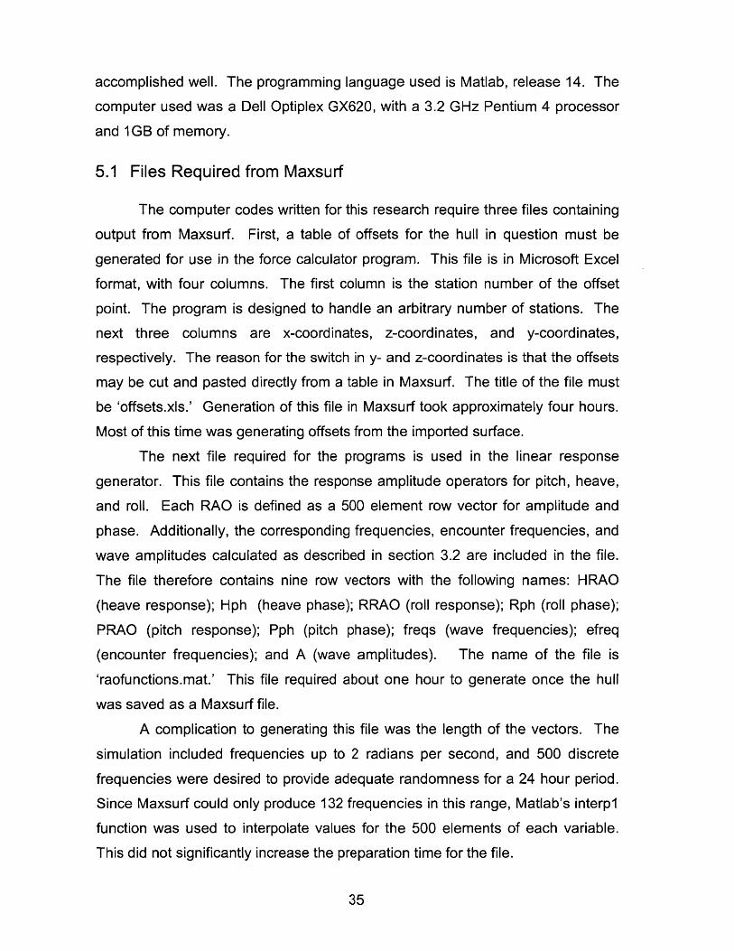
Finally, the righting moment lookup table is required. This is a three-

dimensional lookup table with reference values for each index. The method for

generating the lookup table utilized Maxsurf's Hydromax module. At each draft,

pitch was fixed at values from 20m by the stern to 20m by the bow (+/- .133

radians. This ensures all reasonable values of pitch angle in the time simulation

can be accommodated. The data was collated in a spreadsheet table in the

format shown below:

Displ(kg) LCG(m) VCG(m) T(m)1.6E+07 -10.8 7.5 9

Roll(degrees)Trim(m)

20151050

-5-10-15-20

0000000000

Displ(kg) LCG(m) VCG(m) T(m)1.5E+07 -10.625 7.5 8.75

Roll(degrees)Trim(m)

20151050

-5-10-15-20

0000000000

Table 5-1: Righting Moment vs. Roll, Pitch, & Draft

The table contains restoring moment divided by the acceleration due to

gravity (mass times righting arm) for each value of heave, pitch, and roll. The

two-dimensional table of righting moment as a function of roll and pitch are a two-

dimensional table for the ith set of the variable RM. The index vectors contain the

sequential values of trim, roll, and draft. The titles of these vectors are drafts,

pitchs, and rolls. The pitch is in radians from high to low, while the roll is in

36

10314326230794402584815185085515955651771077218592423135692058278

10320808631463922544876180454815423491712007206674822055592005054

20611101361269685552565424420236857544004867465904945314043893178

20624651362619375537033414891935782493855872439569443648473825025

30872773989511188647961769062267971067068352719599763982145408964

30891477791461298745118755751066012536755488694057062465135336527

40107541061121682011312554111370421077006210227570917449777704006462037

4010966101114596521152134611197453106113609948150896104776500516385324

ig

radians from 0 to 1.74 radians. Drafts are in 0.25 meter increments from two

meters to nine meters. This file is used in the non-linear response generator.

The entire file for nine pitches, eleven roll angles, and 29 drafts took

approximately eight hours to compile.

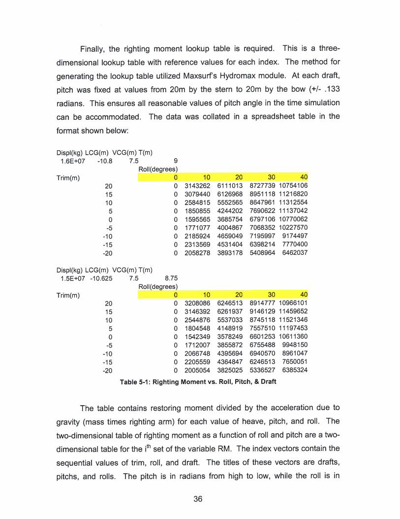
5.2 Excitation Force Calculator

The Matlab program ForceFinder calculates the linear excitation moment

of a ship from offsets provided in an external file using the theory presented in

Chapter Four. The program is designed to calculate the Froude-Krylov and

Diffraction excitation moments for a user defined number of different frequencies.

As mentioned, the program requires a table of offsets with points designated in

meters from the origin. At each frequency, the program determines sectional

moments per unit length of the ship at each section. These sectional moments

are then integrated over the length of the ship to obtain the three dimensional

excitation force. A block diagram of the program is shown in figure 5.1.

Start Endeo

bnt ies 4n1 N nn=nn+1 -

Variable variabqe

set w, we, k freq

sta=1

statta+ Ninert

nstamoments

Call Determine Sectionfindfk Offsets

Figure 5-1: ForceFinder Block Diagram

ForceFinder uses several subroutines to determine the sectional

moments. The main subroutine is 'findfk'. This subroutine takes a section's

37

offsets, determines the sectional excitation moments for the frequency passed to

it. First, it generates the domain shown in figure 4-2 using the subroutine

'setpans'. Next, the subroutine 'infIcoef' calculates the integrals of Green's

function and its derivative at each point due to every other point. The subroutine

'findmatrix' uses these values and the boundary conditions to calculate the

equations for determination of the diffraction potential. With the diffraction

potential known, the subroutine calculates both the Froude-Krylov and diffraction

moments through numerical integration.

Although this process is straightforward, a block diagram of findfk is

presented in figure 5-2. The code for ForceFinder, findfk, and findmatrix are

included in section 1 of Appendix A.

FromMain Return

Apply BC'sTo find matrix(findmatrix)

Figure 5-2: findfk Block Diagram

For the research program, the program was set to generate excitation

moments at 500 frequencies equally divided from zero to 2 radians per second.

This matches the number of wave amplitudes generated for the linear response

spectrum. In this way, the random phasing in the linear response may be applied

to the excitation moments as well. At each frequency, the moment and

amplitude for a one meter wave was calculated. The result is a complex number,

which may be interpreted as a modulus of moment and a phase relative to the

38

GenerateDomain Panels

(setpans)

Calculatef4 and h4

Calculate influenceCoefficients

(inflcoef)cPd=A\b

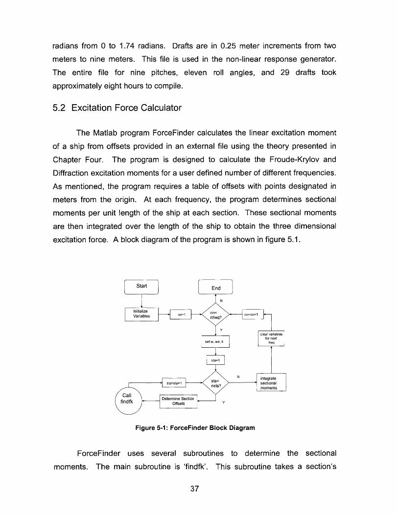
wave height amidships. The output of the program was saved as a Matlab data

file titled 'forcedata500.mat' for use in the non-linear time simulations. The

excitation moment per unit wave amplitude for Sea State Eight is shown in figure

5-3:

x 10612 7I

Froude-Krylov Moment

Diffraction Moment1 0

E8-

C

54-CL

0)E0

00 0.2 0.4 0.6 0.8 1 1.2 1.4 1.6 1.8 2

Circular Frequency (rad/s)

Figure 5-3: Excitation Moments for Seakeeping Problem

ForceFinder has the largest run time of the three programs described.

Because of the large number of panels in the diffraction boundary value problem,

the program requires approximately 50 seconds to find the total excitation force

for each frequency. To match the 500 frequencies used in the spectrum

response calculator, the program run time was 6.9 hours. The author

acknowledges there are many programs available to evaluate the excitation force

that are faster. These may be used as long as the output is in the form of a

Matlab vector labeled F4 containing complex force magnitudes and is saved as

'forcedata500'.

39

5.3 Linear Response Generator

The name of the linear response program is LinearResponse. Although it

does not need any subroutines to operate, it does need the file 'raofunctions.mat'

to generate a time simulation of heave, pitch, and roll. Although only the heave

and pitch vs. time are required for use in the non-linear program, the roll was

calculated for comparison to the time simulation generated in the non-linear roll

simulation.

The linear response program and force program should be run with the

same set of frequencies in their spectra. The linear response program calculates

the wave amplitudes and random phases for each frequency in the simulation.

The moments found in ForceFinder have a phase relative to the phase of their

respective discrete wave system. If the frequencies are not matched prior to

running the two programs, a certain amount of interpolation must happen to

synchronize the frequencies before the final program can be run. This extra work

is easily avoidable by using the same set of frequencies for the separate

programs.

The linear response program is quite simple. For each time, the response

may be expressed as a sum of the linear response at each frequency. This may

be written as# freq

77 = E Ai jH(cqj)jcos(coit + y/i + a) j=3,4,5 (5.1)i=1

The file raofunctions.mat described in section 5.1 contains the wave

amplitudes, transfer function moduli, and transfer function phase angles for these

calculations. Therefore, the program generates a random phase angle for each

frequency, and performs the summation of discrete responses at each time to

produce a wave height, pitch angle, roll angle, and heave.

The output of this program is the time series simulations of wave height,

pitch, heave and roll. Also in the data set will be the frequencies, encounter

frequencies, and wave amplitudes for the sea simulation. The output was saved

as a file titled 'linresplOO.mat' for use in the non-linear response simulation

program. Sample graphs of the time simulations were shown previously in

40

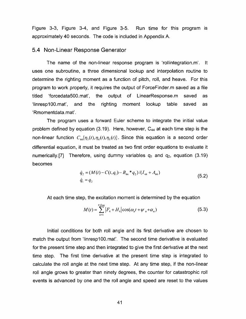
Figure 3-3, Figure 3-4, and Figure 3-5. Run time for this program is

approximately 40 seconds. The code is included in Appendix A.

5.4 Non-Linear Response Generator

The name of the non-linear response program is 'rollintegration.m'. It

uses one subroutine, a three dimensional lookup and interpolation routine to

determine the righting moment as a function of pitch, roll, and heave. For this

program to work properly, it requires the output of ForceFinder.m saved as a file

titled 'forcedata500.mat', the output of LinearResponse.m saved as

'linrespl00.mat', and the righting moment lookup table saved as

'Rmomentdata.mat'.

The program uses a forward Euler scheme to integrate the initial value

problem defined by equation (3.19). Here, however, C44 at each time step is the

non-linear function C44 [773(t), 4 (t),775(t)]. Since this equation is a second order

differential equation, it must be treated as two first order equations to evaluate it

numerically.[7] Therefore, using dummy variables q1 and q2, equation (3.19)

becomes

42 =(M(t) -C(t,q 1)- B44 * q2 )/(I4 +A4) (5.2)41 = q2

At each time step, the excitation moment is determined by the equation#freq

M(t)= ±F4+H4 cos(Cot+,+a,,) (5.3)n=1

Initial conditions for both roll angle and its first derivative are chosen to

match the output from 'linrespl00.mat'. The second time derivative is evaluated

for the present time step and then integrated to give the first derivative at the next

time step. The first time derivative at the present time step is integrated to

calculate the roll angle at the next time step. At any time step, if the non-linear

roll angle grows to greater than ninety degrees, the counter for catastrophic roll

events is advanced by one and the roll angle and speed are reset to the values

41

of the linear integration at for that time. The block diagram for this program is

shown in Figure 5-4.

LoadStart linrespOO

forcedata500Rmomentdata

Set 0(1),0(1) fromvector 'roll'

m(m+1) = (m)*dt

0(m+1) = 0(m)*dt

m=1

0(m) = (M(m) - C(m) - B * (m)) /(1, + A4 4 )

End m<npts-l?

C(m) 9.8* RightingMoment(draft(m), pitch(m),theta(m))

PM(M)= (F4n + H4n)* A,* COS(a)nt(M) + Vf+ +an)

Figure 5-4: Block Diagram for Non-Linear Roll Integration

An additional capability written into the program is to conduct the

integration using the same linear restoring coefficient that Maxsurf's Sea Keeper

module uses, using equation(3.24). The linear and non-linear integration occur

in the same loop, so little extra computation time is required for this addition. The

programs as written in Appendix A are designed to use 500 frequencies up to a

value of 2 radians per second to integrate the roll equation for one hour using a

time step of 0.01 seconds. The run time for rollintegration is approximately one

minute. The small time step is required for numerical convergence. For such a

small time step, the Forward Euler method gives very nearly the same results as

more complicated integration schemes such as Fourth Order Runge-Kutta.

Convergence with a larger time step for implicit integration rules remains to be

investigated for solving the roll differential equation.

42

6 Simulation Results

6.1 Sea Keeper and Linear Integration Simulations

The first comparison that can be made using the output of the integration

program is between the Sea Keeper module of Maxsurf and the integration using

the linear forces and a linear restoring coefficient. As noted in section 3.4, Sea

Keeper uses an approximation of wave slope times the hydrostatic restoring

coefficient for its excitation force. To compare the two excitation forces, the

output from the ForceFinder program was normalized by the value of the Sea

Keeper excitation force (kAC44). This comparison is shown in Figure 6-1. The

figure shows the normalized modulus of the excitation force vs frequency, along

with the constant value of kAC44 that Sea Keeper uses as its excitation force. The

largest discrete wave heights will be near the modal frequency, which is also

shown in the figure.

0.6 0.8 1o (rad/s)

1.2 1.4 1.6 1.8

Figure 6-1: Modulus of Non-dimensional Excitation Force vs. Frequency

The phase angles of the excitation forces are not shown. Since the

calculated excitation moment is computed as a complex number, the phase

varies with the frequency of the wave. On the other hand, the Sea Keeper

43

1.4

1.2

1

0.8

0.6

0.4

0.2

0

LL

Force Finder

- Sea Keeper

- Modal Frequency,Sea State Eight

0 0.2 0.4 2

excitation moments do not include a phase shift, assuming that the excitation

force always acts in phase with the wave height. While this assumption may be

valid for longer wavelengths, it does not hold true for shorter waves. This

difference does not significantly affect the amplitude of the response.

The modulus of the calculated force is larger in the area of the largest

discrete wave heights. Therefore, the overall calculated force should be larger

than the estimations used by Sea Keeper. The linear integration uses the same

value of C4 as the Sea Keeper program. Therefore, the only difference of the

time series for roll between the integration scheme and Sea Keeper is the

excitation forces. The larger forces in the integration should result in a larger

average amplitude for roll response. This is in fact the case. The average

amplitude was determined by calculating the standard deviation of the time

series of the two different methods. The amplitude of the Sea Keeper time series

was 8.8 degrees, while the linear integration average amplitude was 11 degrees.

A plot of the first five minutes is shown in Figure 6-2 for comparison of the two.

30

20

0)C)

10

0

-10

-20

-30'0 2

Time (minutes)3 4 5

44

Linear RollSea Keeper Roll ~

I

OR, - - -- " --- - ----- .. .. .... ------

1

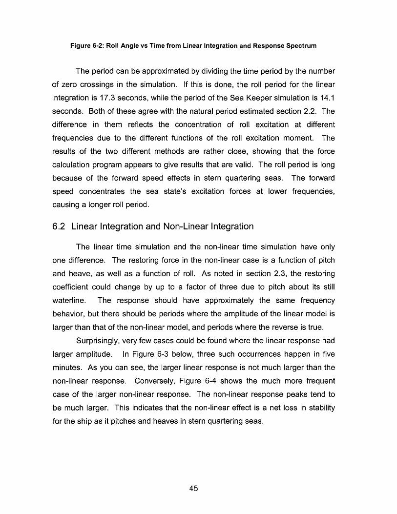
Figure 6-2: Roll Angle vs Time from Linear Integration and Response Spectrum

The period can be approximated by dividing the time period by the number

of zero crossings in the simulation. If this is done, the roll period for the linear

integration is 17.3 seconds, while the period of the Sea Keeper simulation is 14.1

seconds. Both of these agree with the natural period estimated section 2.2. The

difference in them reflects the concentration of roll excitation at different

frequencies due to the different functions of the roll excitation moment. The

results of the two different methods are rather close, showing that the force

calculation program appears to give results that are valid. The roll period is long

because of the forward speed effects in stern quartering seas. The forward

speed concentrates the sea state's excitation forces at lower frequencies,

causing a longer roll period.

6.2 Linear Integration and Non-Linear Integration

The linear time simulation and the non-linear time simulation have only

one difference. The restoring force in the non-linear case is a function of pitch

and heave, as well as a function of roll. As noted in section 2.3, the restoring

coefficient could change by up to a factor of three due to pitch about its still

waterline. The response should have approximately the same frequency

behavior, but there should be periods where the amplitude of the linear model is

larger than that of the non-linear model, and periods where the reverse is true.

Surprisingly, very few cases could be found where the linear response had

larger amplitude. In Figure 6-3 below, three such occurrences happen in five

minutes. As you can see, the larger linear response is not much larger than the

non-linear response. Conversely, Figure 6-4 shows the much more frequent

case of the larger non-linear response. The non-linear response peaks tend to

be much larger. This indicates that the non-linear effect is a net loss in stability

for the ship as it pitches and heaves in stern quartering seas.

45

30 - 1Larger Linear Response

20-

10

0

5 -10-C

-20-

-30-

non-linear time series-4__-_- linear time series

-40-

40 41 42 43 44 45Time (minutes)

Figure 6-3: Linear Simulation vs. Non-linear Simulation with Larger Rolls in the LinearCase

The period of the two integration schemes were very similar. While the

linear integration period was 17.3 seconds, the non-linear time series showed a

period of 17.0 seconds. The amplitudes of the responses were quite different,

however. As noted before, the standard deviation of the linear series was 11

degrees. The non-linear roll had a standard deviation of 16.9 degrees, which is

an increase of more than fifty percent. With larger roll amplitude and the same

period, this implies much greater roll speed and acceleration. Therefore not only

is the hull less stable when treated in a non-linear fashion, it would be less

comfortable for crew as well.

46

90 -------

0

-90

2 5

III II

1 32 33 34

Figure 6-4:Linear Simulation vs. Non-linear Simulation with Larger Rolls in the Non-linearCase

Examination of Figure 6-4 shows a phenomenon that is unique to the non-

linear case. The roll angle exceeds ninety degrees. This large of a roll angle

exceeds the ability of the program to determine the righting moment, and can be

called a catastrophic roll event. This hull form may have a positive righting

moment at roll angles of more than ninety degrees, but a roll of more than ninety

degrees could be catastrophic nonetheless for two reasons. First, anything

inside the ship that is not tied down will undoubtedly move towards the

furthermost hull. Among other problems this represents, the change in the center

of gravity will cause an upsetting moment within the ship. The second

undesirable effect would be downflooding. The downflood angles of this hull

design are not designated, but immersing half of the main deck and

superstructure should almost certainly cause down flooding even for roll angles

less than 90 degrees.

47

(D

L.

non-linear time serieslinear time series

-Caastc- - --- E t-- -

h Catastrophic EEnnt

----- Catastrophic Event- - ------- ------------------------------------------- - -

KJI I I I I

26 27 28 29 30 3Time (minutes)

35

. .. .. . ...... ..

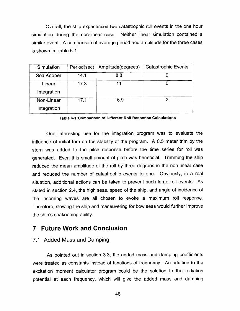
Overall, the ship experienced two catastrophic roll events in the one hour

simulation during the non-linear case. Neither linear simulation contained a

similar event. A comparison of average period and amplitude for the three cases

is shown in Table 6-1.

Simulation Period(sec) Amplitude(degrees) Catastrophic Events

Sea Keeper 14.1 8.8 0

Linear 17.3 11 0

Integration

Non-Linear 17.1 16.9 2

Integration

Table 6-1:Comparison of Different Roll Response Calculations

One interesting use for the integration program was to evaluate the

influence of initial trim on the stability of the program. A 0.5 meter trim by the

stern was added to the pitch response before the time series for roll was

generated. Even this small amount of pitch was beneficial. Trimming the ship

reduced the mean amplitude of the roll by three degrees in the non-linear case

and reduced the number of catastrophic events to one. Obviously, in a real

situation, additional actions can be taken to prevent such large roll events. As

stated in section 2.4, the high seas, speed of the ship, and angle of incidence of

the incoming waves are all chosen to evoke a maximum roll response.

Therefore, slowing the ship and maneuvering for bow seas would further improve

the ship's seakeeping ability.

7 Future Work and Conclusion

7.1 Added Mass and Damping

As pointed out in section 3.3, the added mass and damping coefficients

were treated as constants instead of functions of frequency. An addition to the

excitation moment calculator program could be the solution to the radiation

potential at each frequency, which will give the added mass and damping

48

coefficients for use in the non-linear integration problem. The frequency

dependent added mass and damping can be calculated by a numerical problem

very similar to that used to find the diffraction force[6]. Only the boundary

conditions on the ship surface are different.

7.2 Directional Seas

The waves that are simulated in this thesis are long-crested waves

assumed to be from a distant storm. Simulation of multidirectional random seas

may be included in this analysis through methods described in previous research

from Mr. Sam Geiger[8]. The unidirectional spectrum could be replaced with a

sum of several unidirectional seas with different headings, all adding up to the

same energy as the single unidirectional sea state. This inclusion would provide

a better estimate of the excitation forces involved in real seas.

7.3 Non-linear Excitation Moments

The Froude-Krylof and Diffraction excitation moments were calculated

using linear strip theory along the still waterline of the ship's hull. In reality, the

moments will depend on the actual waterline of the ship as the waves travel in

space. The moment will also depend on the amount of the hull in the water as

the ship is displaced in roll, heave, and pitch. Calculation of these effects is left

as a topic of further research.

7.4 Wave Profile Effects on Righting Moment

The righting moment for the tumblehome hull was calculated using the

draft of the ship at amidships, assuming no effects for wave height or wave

slope. The draft at other positions along the length of the ship is a function of the

longitudinal wave height and the pitch of the ship relative to the wave slope.

Therefore, the righting moment may be refined by taking these two factors into

consideration.

7.5 Conclusion

49

The non-linear roll integration program developed in this thesis can

provide an estimate of the roll response for any hull, given its offsets and the

righting moment data. Although the force calculation program takes some

computation time, any available program that determines the excitation force

may be used to give the roll integration program its input. The program could be

used in any number of design applications, such as determination of a safe

operating envelope for a ship, or the effects of different trim configurations on

stability. Most importantly, it provides a non-linear simulation in a relatively short

time using only a desktop computer. This fact makes the computer program a

valuable design tool.

50

List of References

[1]. Cavas, Christopher, "Dangerous New Design?," Navy Times, 9 April 2007.[2]. Belknap, W & Campbell, B. "ONR Topside Hull-forms", February 2005.[3]. Salveson, N., E.O.Tuck & 0. Faltinsen (1970), "Ship motions and Sea

Loads," SNAME Transactions, Volume 78, 1970.[4]. Formation Design Systems, Maxsurf Operators Manual. 2004.[5]. Lewis, Edward Ed. Principles of Naval Architecture, Voll ///. Jersey City,

NJ: Society of Naval Architects & Marine Engineers, 1989.[6]. Milgram, Jerome. "Strip Theory for Underwater Vehicles in water of Finite

Depth," Journal of Applied Mathematics, in press 2007.[7]. Chapra, Steven C. and Raymond P. Canal. Numerical Methods for

Engineers (Second Edition). New york: McGraw-Hill, 1988.[8]. Geiger, Sam "Hydrodynamic Modeling of Towed Bouyant Submarine

Antenna's in Multidirectional Sea." Master's Degree thesis, MassachusettsInstitute of Technology, Cambridge, Massachusetts, 2000.

51

Appendix A: Matlab Code for Finding Excitation Forces

1. Main Program: 'ForceFinder.m' - This program needs the followingsubroutines to function : findfk, findmatrix, setpans, inficoef, rank2d, localize.Also needs a Microsoft Excel file with offsets provided as described in theprogram. The m-files inficoef, rank2d, and localize were provided by ProfessorJerome Milgram.

% Finds Froude-Krylov and Diffraction Excitation Moments% for frequencies up to 2.5 rad/s, unit amplitude wave% Requires the following files to operate:% offsets.xls: table of offsets in MS Excel with the following columns:% Col 1: station number (can handle any number of stations)% Col 2: x-values (m)% Col 3: z-values (m)% Col 4: y-values (m)% Subroutines: findfk, findmatrix, setpans, inflcoef, rank2d, localize% # of frequencies is set by nfreq% output is in the variables F4, H4% for the research, set nfreq to 500, save data as forcedata500

clear allclose alltictimestampb=clock;starttime=timestampb(4)*1 00+timestampb(5);fprintf('start time =%1.0f\n',starttime)

% initialization of variables:% rho: density of seawater (kg/mA3)% nsta: # of stations (from offsets file)% B: beam of ship (m)% gr: acceleration due to gravity% npts: number of offsets% U: forward speed of the ship% nfreq: number of frequencies in interval 0:2.5% F4: Foude Krylov excitation moment% H4: Diffraction excitation moment% wo, we, k: stationary frequency, encounter frequency, wave number% T: draft% beta: angle of incidence of waves

rho=1025;A= xsread('offsets');nsta=max(A(:,1));B=2*max(A(:,3));gr=9.8;

52

... .... ... ... .. ...

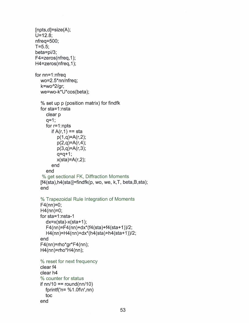
[npts,d]=size(A);U=12.8;nfreq=500;T=5.5;beta=pi/3;F4=zeros(nfreq,1);H4=zeros(nfreq,1);

for nn=1:nfreqwo=2.5*nn/nfreq;k=woA2/gr;we=wo-k*U*cos(beta);

% set up p (position matrix) for findfkfor sta=1:nsta

clear pq=1;for r=1:npts

if A(r,1) == stap(1,q)=A(r,2);p(2,q)=A(r,4);p(3,q)=A(r,3);q=q+1;x(sta)=A(r,2);

endend

% get sectional FK, Diffraction Moments[f4(sta),h4(sta)]=findfk(p, wo, we, k,T, beta,B,sta);end

% Trapezoidal Rule Integration of MomentsF4(nn)=O;H4(nn)=O;for sta=1:nsta-1

dx=x(sta)-x(sta+1);F4(nn)=F4(nn)+dx*(f4(sta)+f4(sta+1))/2;H4(nn)=H4(nn)+dx*(h4(sta)+h4(sta+1))/2;

endF4(nn)=rho*gr*F4(nn);H4(nn)=rho*H4(nn);

% reset for next frequencyclear f4clear h4% counter for statusif nn/10 == round(nn/10)

fprintf('n= %1.0f\n',nn)toc

end

53

. .. . ... .......

endtoc

l.a. Subroutine: 'findfk.m'

function [f4, h4] = findfk(p, w, we, k, T, beta,B,sta)% Finds sectional Froude Krylov & Diffraction Excitation Moments for% ForceFinder% p is matrix of offsets, a is incremental waveheight, psi is random phase angle,w,k are freq & wave nr%KG is height of cg above baseline T is still water draft%posit(1,:) are y-values, posit(2,:) are z values in the section plane%x is the longitudinal position of the section%beta is the angle of incidence of the incoming wave, measured in radians fromthe stern%etal & eta2 are the actual waterlines of the ship after translation andapplication of the wave%r & q are the point indices corresponding to etal & eta2%f2 & f3 are the two-d F-K forces for the section%posit is a matrix of y,z ordered pairsposit(1,:)=p(2,:);posit(2,:)=p(3,:);x=p(1,1);[d,npts]=size(posit);posit(3,:)=zeros(1,npts);gr=9.8;cl=gr/w;c2=k*x*cos(beta);c3=k*posit(2,:)-T;

% This block of code calculates the 2dimensional diffraction potential for thesectionnpv=1 0;nph=55;npb=1 0;% defines domain for constant panel method[np,npanels,yvert,zvert,ybv,zbv,ycontrol,zcontrol,lgth,ny,nz] =setpans(posit(1,:),posit(2,:)-T,npv,nph,npb,B,k,T);% finds G, dG/dn for each panel[g, dgdn] = inflcoef(npanels,yvert,zvert,ycontrol,zcontrol,igth);% finds A & b in discrete BVP A(phi)=b[Amatrix,b] =findmatrix(np,nph, npv,n pb,w,we, k, beta,x,ycontrol,zcontrol,ny, nz,g,dgd n);phid=Amatrix\b;

% determines total disturbance potentialfor m=1:np-1

phil=c1 *exp(i*(c2+k.*sin(beta)*posit(2,m)))*exp(c3(m));PSI4(m)=phil+phid(np+nph-1 +m);

54

phil=cl *exp(i*(c2-k.*sin(beta)*posit(2,m)))*exp(c3(m));PSI4Ieft(m)=phil+phid(np+nph-m);

end

%Translation to origin, which is still water WLposit(2,:)=posit(2,:)-T;WL=O;f4=0;h4=0;

% q is number of points below waterlineif min(posit(2,:))>WL

fprintf('station is above water\n')return

endif max(posit(2,:))>WL

q=1;while posit(2,q)<WL

q=q+1;endq=q-1;fprintf('%1.2f out of %1.2f points\n',q,npts-1)

elseq=npts-1;fprintf('station is below water\n')

endr=q;

aa=zeros(3,npts);%find forces on 'the right half of the hullfor j=1:q

% compute normalsaa(:,j)=cross(posit(:,j+1)-posit(:,j),[O;O;-1]);amag=sqrt(aa(1,j)A2+aa(2,j)A2);n3(j)=aa(1,j)/amag;n2(j)=aa(2,j)/amag;mid=(posit(:,j)+posit(:,j+1))/2;n=[n2(j) n3(j) 0];n4v=cross(mid,n);n4(j)=n4v(3);

z1 =posit(2,j);z2=posit(2,j+1);dl=sqrt((posit(1,j)-posit(1,j+1))^2+(posit(2,j)-posit(2,j+1 ))^ 2);

% calculate the incremental excitation momentptl =exp(k*posit(1 j)*sin(beta)*i)*exp(k*z1)*exp(-i*k.*x*cos(beta));pt2=exp(k*posit(1 ,j+ 1 )*sin(beta)*i)*exp(k*z2)*exp(-i*k.*x*cos(beta));

55

- ------------- ..........

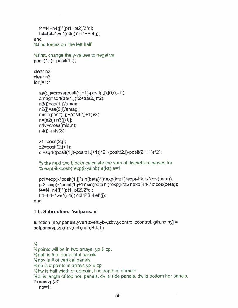
f4=f4+n4(j)*(pt1 +pt2)/2*dl;h4=h4-i*we*(n4(j))*dl*PSl4(j);

end%find forces on 'the left half

%first, change the y-values to negativeposit(1,:)=-posit(1,:);

clear n3clear n2for j=1:r

aa(:,j)=cross(posit(:,j+1)-posit(:,j),[O;O;-1]);amag=sqrt(aa(1 ,j)A2+aa(2,j)A2);n3(j)=aa(1,j)/amag;n2(j)=aa(2,j)/amag;mid=(posit(:,j)+posit(:,j+1))/2;n=[n2(j) n3(j) 0];n4v=cross(mid,n);n4(j)=n4v(3);

z1 =posit(2,j);z2=posit(2,j+1);dl=sqrt((posit(1,j)-posit(1,j+1))A2+(posit(2,j)-posit(2,j+1))A2);

% the next two blocks calculate the sum of discretized waves for% exp(-ikxcosb)*exp(ikysinb)*e(kz),a=1

ptl =exp(k*posit(1 j)*sin(beta)*i)*exp(k*z1 )*exp(-i*k.*x*cos(beta));pt2=exp(k*posit( ,j+1 )*sin(beta)*i)*exp(k*z2)*exp(-i*k.*x*cos(beta));f4=f4+n4(j)*(pt1 +pt2)/2*dl;h4=h4-i*we*(n4(j))*dl*PSl4left(j);

end

I.b. Subroutine: 'setpans.m'

function [np,npanels,yvert,zvert,ybv,zbv,ycontrol,zcontrol,Igth, nx,ny] =setpans(yp,zp,npv,nph,npb,B,k,T)

%points will be in two arrays, yp & zp.%nph is # of horizontal panels%npv is # of vertical panels%np is # points in arrays yp & zp%hw is half width of domain, h is depth of%dl is length of top hor. panels, dv is sideif max(zp)>0

np=1;

56

domainpanels, dw is bottom hor panels.

d=0;while zp(np)<0

np=np+1;endyp=yp(1:np);zp=zp(1:np);dy=yp(np)-yp(np-1);dz=zp(np)-zp(np-1);ynew=yp(np)-zp(np)*dy/dz;yp(np)=ynew;zp(np)=0;

endif max(zp)<=0

[d,np]=size(yp);end

% sets the domain size: hw is half-width (10 beams)% h is depth: half the wavelength or three times the draft,% whichever is greater.% for the ONR hull, B=18.8m ->hw=188m, nph=55, dl=1.54m

hw=10*B;h1 =3/k;h2=3*T;h=max(hl,h2);dl=(hw-yp(np))/nph;dv=h/npv;dw=2*hw/npb;yvert(1)=-hw;zvert(1 )=0;

% vertices for free surfacefor m=1:nph

% left top halfyvert(m+1)=yvert(m)+dl;zvert(m+1)=0;

% right top halftrh=2*np+nph-1 +m;yvert(trh)=yp(np)+dl*m;zvert(trh)=0;

end

% vertices for hullcounter=np;for m=1:np

yvert(m+nph)=-yp(counter);zvert(m+nph)=zp(counter);counter=counter-1;

57

-- - ------- -

mid=m+nph+np-1;yvert(mid)=yp(m);zvert(mid)=zp(m);

end

%vertices for sidesfor m=1:npv

right=2*np+2*nph+m-1;left=right+npv+npb;yvert(right)=hw;zvert(right)=-m*dv;yvert(left)=-hw;zvert(left)=-h+m*dv;

end

% vertices for bottomfor m=1:npb

bot=m+2*np+2*nph+npv-1;yvert(bot)=hw-dw*m;zvert(bot)=-h;

end

endpt=2*(np+npv+nph)+npb-1;yvert(endpt)=yvert(1);zvert(endpt)=zvert(1);npanels=endpt-1;

% control pointsfor k=2 :endpt;

ycontrol(k-1) = 0.5*(yvert(k-1)+yvert(k));zcontrol(k-1) = 0.5*(zvert(k-1)+zvert(k));Igth(k-1)=sqrt((yvert(k)-yvert(k-1 ))A2 ...

+(zvert(k)-zvert(k-1 ))A2);nx(k-1)= -(zvert(k)-zvert(k-1))/lgth(k-1);ny(k-1) = (yvert(k)-yvert(k-1))/Igth(k-1);

end

nbv=endpt-(2*np-3);ybv(1:nph+1)=yvert(1:nph+1);zbv(1:nph+1)=zvert(1:nph+1);ybv(nph+2:nbv)=yvert(2*np+nph-1 :endpt);zbv(nph+2:nbv)=zvert(2*np+nph-1:endpt);

1.c. Subroutine: 'findmatrix.m'

function [Amatrix,b] =findmatrix(np,nph,npv,npb,w,we,k,beta,x,yc,zc,ny,nz,g,dgdn)% x is longitudinal position of station

58

% initialize variablesgr=9.81;ci =i*gr/w;c2=k*x*cos(beta);npanels=2*nph+2*np+2*npv-2+npb;b=zeros(npanels,1);Amatrix=zeros(npanels, npanels);

for m=l:npanelsfor n=l:nph

% top left surface; wA2phi-gdphi/dn=O;

Amatrix(m,n)=dgdn(m,n)-wA2/gr*g(m,n);

%top right surface; same boundary conditionnn=n+2*np+nph-2;Amatrix(m,nn)=dgdn(m,nn)-wA2/gr*g(m,nn);

end

for n=nph+1:2*np+nph-2%ship's hull; dphi/dn=-dphl/dnAmatrix(m,n)=dgdn(m,n);phil=cl *exp(i*(c2-k*sin(beta)*yc(n-nph))+k*zc(n-nph));vv=-phil*i*k*sin(beta);ww=k*phil;vdotn=vv*ny(n-nph)+ww*nz(n-nph);b(m)=b(m)-g(m,n)*vdotn;

endfor n=1:npv

%right side dphi/dn=-ikphinn=n+2*nph+2*np-2;Amatrix(m,nn)=dgdn(m,nn)+i*k*g(m,nn);%left side same boundary conditionnn=n+2*nph+2*np-2+npv+npb;Amatrix(m,nn)=dgdn(m,nn)+i*k*g(m,nn);

endfor n=1:npb

%bottom dphi/dn=Onn=n+2*nph+2*np-2+npv;Amatrix(m,nn)=dgdn(m,nn);

endAmatrix(m,m)=Amatrix(m,m)+pi;

end

2. Main Program: LinearResponse This program only needs theraofunctions.mat file to run.

% Calculates Time simulations for heave, pitch, and roll

59

-Ad

% Needs raofuncations.mat to run

% raofunctions has the following row vectors:

% freqs (wave frequencies of interest)

% efreq (encounter frequencies at each wave frequency)

% A (wave amplitudes at each wave frequency)

% RRAO (roll RAO)

% Rph (roll phase in degrees)

% HRAO (heave RAO)

% Hph (heave phase in degrees)

% PRAO (pitch RAO)

% Pph (pitch phase in degrees)

% save output as linresp100

clear

close all

load raofunctions

tic

[b,a]=size(Hph);

Hph=Hph*pi/1 80;

Pph=Pph*pi/1 80;

Rph=Pph*pi/1 80;

k=freqs.A2/9.8;

we=efreq;

% allow for more than one run for statistics

runs=1;

tinc=1 00;

dt=1/tinc;

% previous two lines set dt to 1/tinc seconds

npts=3600*tinc;

60

. ... .... ..... ... .. ... .... .... ... ......

t=(1:npts)*dt;

heave=zeros(npts,1);

pitch=zeros(npts, 1);

roll=zeros(npts,1);

wh=zeros(npts,1);

for n=1:runs

% set new random phase angles for discretized waves

rand('state',sum(1 00*clock));

psi=2*pi*rand(length(A),1)';

for m=1:npts

wh(m)=sum(A.*cos(efreq*t(m)+psi));

heave(m)=su m(A.*H RAO.*cos(abs(efreq)*t(m)+psi+H ph));

pitch(m)=su m(k.*A.*PRAO.*cos(abs(efreq)*t(m)+psi+Pph));

rolI(m)=sum(k.*A.*RRAO.*cos(abs(efreq)*t(m)+psi+Rph));

if m/tinc==round(m/tinc)

time=m/tinc

toc

end

end

draft=5.5+wh-heave;

maxd raft(n)=max(d raft);

mindraft(n)=min(draft);

n

toc

end

3. Main Program: rollintegration:

% Integrates exciting forces over time to produce a time sim of roll angle% Needs RightingMoment.m to run% Needs the following files to run:% Rmomentdata.mat:% Contains data to conduct the lookup table function for righting moment% forcedata500.mat: Output of ForceFinder, saved as a .mat file

61

% linresp1 0O.mat: Output of LinearResponse, saved as .mat file

clear allclose all

global RMglobal rollsglobal draftsglobal pitchsticload Rmomentdataload forcedata500load linresp100

% sets the time simulation to npts*dt secondsnpts=360000;dt=.01;

% Sets the moment of inertia, added inertia, damping% and linear restoring coefficientsmass=8402180;lactual=mass*(.4*B)A2;A44=.3*lactual;I=Iactual+A44;b=.075;c44=1.476*mass*gr;B44=b*sqrt(c44*1);

% initialize the catastrophic roll event countercount=0;

theta=zeros(npts,1);thdot=zeros(npts,1);thddot=zeros(npts,1);theta2=zeros(npts,1);thdot2=zeros(npts,1);thddot2=zeros(npts,1);M=zeros(npts,1);C=zeros(npts,1);C2=zeros(npts,1);% provide the option to trim by the sternpitch=pitch;

% set IC's to match linresp100theta(1)=roll(1);thdot(1)=(roll(2)-roll(1))/dt;theta2(1)=theta(1);thdot2(1)=thdot(1);

62

.. ...................

%Set magnitude and phase of excitation forcesexmoment=abs((F4+H4)'.*A);mphase=angle(F4+H4)';

for m=1:npts-1

M(m)=su m(exmoment.*cos(we*t(m)+psi+mphase));% protect for high pitch valuesif pitch(m)>max(pitchs)

pitch(m)=max(pitchs);end% check for catastrophic roll eventif theta(m)>pi/2

theta(m)=theta2(m);thdot(m)=thdot2(m);count=count+1

endif theta(m)<-pi/2

theta(m)=theta2(m);thdot(m)=thdot2(m);count=count+1

end% Find non-linear restoring momentC(m)=9.8*RightingMoment(d raft(m), pitch(m),abs(theta(m)));if theta(m)<O

C(m)=-C(m);end% Find linear restoring momentC2(m)=c44*theta2(m);

% Forward Euler integrationthddot(m)=(MhoC(m)-B44*thdot(m))/;thdot(m+ 1 )=thdot(m)+thddot(m)*dt;theta(m+ 1)=theta(m)+thdot(m)*dt;

thddot2(m)=(M(m)-C2(m)-B44*thdot2(m))/l;thdot2(m+1)=thdot2(m)+thddot2(m)*dt;theta2(m+1)=theta2(m)+thdot2(m)*dt;

end

t=t/60;figure(1)plot(t(1:m),theta2(1:m)*1 80/pi,t(1:m),roll(1:m)*1 80/pi)figure(2)plot(t(1:m),theta(1:m)*1 80/pi,t(1:m),theta2(1:m)*1 80/pi)

toc

63

% function to determine non-linear roll moment% variable RM is lookup table for righting moments.% RM(:,p,r) is moment vs. draft% RM(d,:,r) is moment vs. pitch% RM(d,p,:) is moment vs. roll% From an excel spreadsheet:

% roll: 0 .05 ...% pitch% -.15 RM(d,-.15,0) RM(d,-.15,.05)% -.1 RM(d,-.1,0) RM(d,-.1,.05)%Y ...

3.a subroutine: 'RightingMoment'

function moment = RightingMoment(heave, pangle, rangle)

global RMglobal draftsglobal pitchsglobal rolls

% protects from high pitch/heaveif heave<2

heave=2endif pangle<-0.1337

pangle=-.1337end

rangle=abs(rangle);

% find heave indexd=1;while drafts(d)<=heave

d=d+1;end% find pitch indexp=1;while pitchs(p)>=pangle

p=p+1;end% find roll indexr=1;while rolls(r)<=rangle

r=r+1;end

% 3-D interpolation

64

... .........

HMRA=RM(d,p,r)-(rolls(r)-rangle)/(rolls(r)-rolls(r-1))*(RM(d,p,r)-RM(d,p,r-1));LM RA=RM(d, p-1, r)-(rolls(r)-rangle)/(rolls(r)-rolls(r- 1))*(RM (d, p-1, r)-RM (d, p-1, r-1));HRA=HMRA-(pitchs(p)-pangle)/(pitchs(p)-pitchs(p-1))*(HMRA-LMRA);HMRA=RM(d-1,p,r)-(rolls(r)-rangle)/(rolls(r)-rolls(r-1))*(RM(d-1,p,r)-RM(d-1,p,r-1));LMRA=RM(d-1, p-1,r)-(rolls(r)-rangle)/(rolls(r)-rolls(r-1))*(RM(d-1,p-1,r)-RM(d-1,p-1,r-1));LRA=HMRA-(pitchs(p)-pangle)/(pitchs(p)-pitchs(p-1))*(HMRA-LMRA);

moment=H RA-(drafts(d)-heave)/(drafts(d)-d rafts(d-1 ))*(H RA-LRA);return

65

Appendix B: List of Symbols

Variable Meaning

A Wave Amplitude

Aik Added MassB Beam

Bik Damping CoefficientCik Restoring Coefficient

Section Froude-Krylovf MomentFi Force In The j Directiong Acceleration Of Gravity

G Green's FunctionSectional Diffraction

h Moment

H Transfer FunctionH4 Diffraction MomentH1/3 Significant Wave Height144 Roll Moment Of Inertiak Wave Number

Ik44 Roll Gyradiust Length

Mik Generalized Mass TermNormal VectorComponent In J

ni DirectionP Pressure

Response AmplitudeRAO OperatorS Wave Spectral Densityt Time

Speed In The X-u Direction

Variable MeaningSpeed In The Y-

v DirectionVelocity Vector

V VolumeSpeed In The Z-

w Directionx Longitudinal Direction

Non-dimensional AddedX44 mass coefficienty Transverse Directionz Vertical Direction

Phase Angle ForTransfer Function or

a MomentWave Angle Of

/3 IncidenceNon-Dimensional

fl44 Damping TermA Displacement

Wave ElevationR; Response Value0 Roll Angle

Tuning Coefficient OrA Wavelengthp Densityc1 Velocity Potential

Diffraction Potential

(PD

01 Incident PotentialWave Phase Angle

qiw Circular FrequencyWe Encounter Frequency

Modal FrequencyWmWO Wave Frequency

66