new challenges to florida citrus: a capital budgeting...
TRANSCRIPT
1
NEW CHALLENGES TO FLORIDA CITRUS: A CAPITAL BUDGETING ANALYSIS OF
THE IMPACT OF CITRUS CANKER, GREENING, AND RURAL LAND PRICES ON
FLORIDA CITRUS GROWERS
By
JORDAN CARTER MALUGEN
A THESIS PRESENTED TO THE GRADUATE SCHOOL
OF THE UNIVERSITY OF FLORIDA IN PARITAL FULLFILLMENT
OF THE REQUIREMENTS FOR THE DEGREE OF
MASTER OF SCIENCE
UNIVERSITY OF FLORIDA
2009
2
© 2009 Jordan Carter Malugen
3
ACKNOWLEDGMENTS
First, to my parents, whose insistence that I finish this work on a timely basis was mostly
ignored but not forgotten. Second, to my good friend and intellectual superior Dr. Fredrick
Houts, whose accomplishments serve as an example of diligence for me and all who know him.
Third, to the University of Florida’s Food and Resource Economics Department and its Chair,
Dr. Thomas H. Spreen, who recruited me and led me into a new discipline that will serve me for
the rest of my life. Fourth, to Professor Ronald Muraro who taught me the nuts and bolts of the
Florida citrus industry. Fifth, to Dr. Charles Moss who always challenged me to expand my
understanding and perception of the world around me and provided valuable advice on writing
this thesis. Sixth, to the University of Florida’s Institute of Food and Agricultural Sciences and
Senior Vice President Jimmy Cheek, who provided me with the financial support and working
environment to complete my work. Lastly, to the people of Florida and the Florida citrus
growers, who made this research possible.
4
TABLE OF CONTENTS
page
LIST OF TABLES .......................................................................................................................... 6
LIST OF FIGURES ........................................................................................................................ 8
ABSTRACT .................................................................................................................................... 9
CHAPTER .................................................................................................................................... 11
1 INTRODUCTION ................................................................................................................. 11
2 ESTABLISHMENT COST, YIELD, AND INVESTMENT PARAMETERS FOR
CITRUS PRODUCTION IN FLORIDA ............................................................................... 15
Modeling Citrus Production .................................................................................................. 15 Grove Care and Operating Cost Considerations .................................................................... 17
3 ACCOUNTING FOR THE EFFECTS OF CITRUS CANKER AND GREENING ON
FLORIDA COMMERCIAL CITRUS PRODUCTION ........................................................ 33
Citrus Canker ......................................................................................................................... 33
Citrus Greening ...................................................................................................................... 38
4 A NET PRESENT VALUE MODEL OF A FLORIDA CITRUS GROVE ......................... 46
Net Present Value Theoretical Framework ............................................................................ 47 Adapting NPV Analysis to the Citrus Grove ......................................................................... 63
5 EMPIRICAL RESULTS ....................................................................................................... 72
Results of the Mixed-Age Grove Model – Yield and Cost Analysis .................................... 72
Results of the Mixed-Age Grove Model – Breakeven Price Analysis .................................. 81
6 SUMMARY AND CONCLUSIONS .................................................................................... 92
APPENDIX ................................................................................................................................... 99
A GEOGRAPHIC AND TOPOGRAPHIC FEATURES OF FLORIDA COMMERCIAL
CITRUS PRODUCTION REGIONS .................................................................................... 99
B PARAMETERS USED IN THE ANALYSIS ..................................................................... 104
C SELECTED RESULTS ....................................................................................................... 117
LIST OF REFERENCES ............................................................................................................ 124
5
BIOGRAPHICAL SKETCH ...................................................................................................... 129
6
LIST OF TABLES
Table page
2-1 Florida citrus marketing by variety, 2005-06 season ............................................................. 21
2-2 Spray budget comparison: fresh versus processed, cost per acre ........................................... 21
3-1 Tree loss percentages used in analysis ................................................................................... 42
3-2 Annual per acre spray costs by disease scenario .................................................................... 45
4-1 Discounting example .............................................................................................................. 54
4-2 Risk adjusted discount rates by variety .................................................................................. 57
4-3 Discount rates used in citrus investment analysis .................................................................. 58
4-4 Built-up capitalization rate method used in analysis .............................................................. 62
4-5 Comparable Florida grove sales ............................................................................................. 63
5-1 Beginning tree age distribution for mature Valencia on the Ridge ........................................ 74
5-2 Initial investment costs by scenario ........................................................................................ 79
5-3 Tree loss percentage by scenario ............................................................................................ 80
5-4 Estimated breakeven prices across disease scenarios, varieties, and production regions ...... 83
5-5 Grapefruit packout price vomparison ..................................................................................... 87
5-6 Hamlin yield-loss sensitivity .................................................................................................. 88
5-7 Tree loss comparison for a Valencia grove on the Ridge with greening ................................ 90
A-2 Average citrus land preparation costs, 2002-03 season ....................................................... 103
A-3 Land utilization of Florida citrus groves ............................................................................. 103
B-1 Solidset costs by disease scenario for a Valencia orange grove in the ridge ....................... 105
B-2 Reset costs by disease scenario for a Valencia located in the ridge .................................... 106
B-3 New planting/replanting operating costs for a Valencia grove (without canker or greening)
................................................................................................................................... 107
B-4 Operating costs for a mature (15+ year old)Valencia grove located on the ridge (without
canker or greening) ................................................................................................... 108
7
B-5 Harvest and other per box costs ........................................................................................... 109
B-6 Adjustment factors for grove care cost by tree age .............................................................. 109
B-7 Annual irrigation expense (ridge/flatwoods comparison).................................................... 110
B-8 Average per acre citrus land preparation costs (ridge/flatwoods comparison) .................... 110
B-9 Property tax levy for top five citrus producing counties, 2003 ............................................ 110
B-10 Property tax analysis assumptions ..................................................................................... 111
B-11 USDA average yields by variety and production district, 1999-2004 average .................. 111
B-12 Rootstock study for Valencia oranges on ridge and flatwoods sites ................................. 112
B-13 Fruit and juice yield by variety used in the analysis .......................................................... 112
B-14 Mature grove production costs with canker by production region .................................... 113
B-15 Mature grove production costs with greening by production region ................................. 114
B-16 Mature grove production costs with canker and greening ................................................. 115
B-17 Spray schedule and costs by variety and disease scenario ................................................. 116
C-1 Tree age distribution of a solidset Valencia grove, base scenario ....................................... 118
C-2 Yields for a solidset Valencia grove- base scenario ............................................................ 119
C-3 Reset strategy beginning/ending tree distributions under disease scenarios ....................... 120
C-4 Estimated breakeven price by scenario ................................................................................ 121
C-5 Average grove production costs by scenario and disease .................................................... 122
8
LIST OF FIGURES
Figure page
2-1 Evolution of Florida citrus grove density (source: 2004-05 Florida Citrus Summary)......... 16
2-2 Working capital illustration ................................................................................................... 29
2-3 Application of working capital to citrus investment ............................................................. 29
3-1 Indonesian citrus production, 1975-2005 .............................................................................. 40
3-2 Thai citrus production, 1975-2005 ........................................................................................ 41
3-3 South Africa citrus production, 1975-2005 ........................................................................... 42
4-1 Relationship of NPV and IRR ............................................................................................... 51
4-2 Tree age distribution matrix .................................................................................................. 64
4-3 Cost calculation by tree age (original trees) .......................................................................... 68
4-4 Reset tree age matrix ............................................................................................................. 69
5-1 Costs and yields for a newly planted Valencia grove on the Ridge ...................................... 74
5-2 Costs and yields for a mature Valencia grove on the Ridge .................................................. 74
5-3 Costs and yields for mature Indian River grapefruit grove with canker ............................... 76
5-4 Costs and yields for mature Hamlin flatwoods grove with greening .................................... 76
5-5 Resetting comparison ............................................................................................................ 77
A-1 Florida commercial citrus acreage map, 2005 .................................................................... 100
A-2 Florida citrus soil types ....................................................................................................... 101
A-3 Illustration of flatwoods grove design ................................................................................ 101
9
Abstract of Thesis Presented to the Graduate School
of the University of Florida in Partial Fulfillment
of the Requirements for the Degree of Master of Science
NEW CHALLENGES TO FLORIDA CITRUS: A CAPITAL BUDGETING ANALYSIS
OF THE IMPACT OF CITRUS CANKER, GREENING, AND RURAL LAND PRICES
ON FLORIDA CITRUS GROWERS
By
Jordan Carter Malugen
August 2009
Chair: Thomas H. Spreen
Major: Food and Resource Economics
The Florida citrus industry provides over $9.2 billion dollars in direct and indirect
expenditures; employs more than 75,000 people, mainly in rural areas; and is an emblematic
feature of the landscape and history of Florida. After the disastrous hurricane seasons of 2004
and 2005, Florida citrus acreage is now at its lowest point since the tracking of citrus tree acreage
first began in 1966, and may decline further due to the twin challenges of diseases known as
citrus canker and citrus greening, and the rapid urbanization of the state. This study conducts an
expansive survey of current growing practices and collects available information regarding costs,
returns, and yields to create a detailed set of parameters. These parameters are analyzed to
determine the economics of an investment in citrus within a net present value framework, and
uses scenario analysis to test for effects on the profitability of a citrus investment due to these
new challenges.
Parameters and assumptions are defined to reflect average costs and yields of a Florida
citrus grove in normal operations and under the scenarios of canker, greening, and increased land
prices. An empirical present value model is created which dynamically reflects the changes in
costs, yields, and tree loss and replacement (resetting) through a fifteen-year period. The
10
analysis examines the citrus investment by looking at: tree yields and costs by variety (Valencia
orange, Hamlin orange, and red grapefruit), age of the grove (new planting versus mature grove),
location (the Central ridge, Southwest Florida flatwoods, and the Indian River regions), the
presence of disease in various severities (canker and greening), and changes in land prices.
The effect of these variables is measured through changes in the breakeven price of one
unit of production (pound solid for oranges or on-tree box for grapefruit). The breakeven price is
defined as the minimum price guaranteeing a positive net present value throughout the fifteen-
year analysis period. Results are presented to help understand how the challenges affecting the
whole industry may affect the investment decisions faced by the thousands of individual
growers, service-providers, and employees who make up this industry and, ultimately, whose
livelihood depends on it.
11
CHAPTER 1
INTRODUCTION
Florida is the largest producer of citrus in the United States, and second only to Brazil in
the entire world. Florida is the second largest producer of orange juice in the world, and the
largest producer of grapefruit. The 2005-2006 Florida citrus crop was estimated at over $1
billion in value, moreover the Florida citrus industry provided over $9.2 billion dollars in direct
and indirect expenditures to the state GDP and employed more than 75,000 people throughout
the state (Spreen et al. 2006). Unfortunately, while the 2005-6 crop was the second highest
valued crop in Florida history due to high prices, the total acreage of Florida citrus fell 17% from
748,555 to 621,373 acres over the last two years. It is now at its lowest point since the tracking
of citrus tree acreage first began in 1966, and may decline further due to the twin challenges of
diseases known as citrus canker and citrus greening, and the rapid conversion of agricultural land
to residential and commercial uses.
These challenges are unfamiliar to Florida growers and contain the possibility of
fundamentally altering the production and cost structure of the Florida citrus industry. Citrus
canker is a bacterial disease of citrus that causes lesions (or cankers) on the fruit and leaves of
citrus trees, reduces tree productivity, and severely affects the marketability of fresh citrus fruit.
Citrus greening is a bacterial disease of citrus that kills trees and is spread by the invasive insect
species, the Asian citrus psyllid. Finally, rapidly expanding Florida population and conversion
of rural lands to urban use have greatly increased the price of agricultural land suitable for citrus
production and is changing the highest and best use of rural land in many traditional citrus
production areas. It appears that these challenges are having an effect on citrus growers, but
there is a lack of economic analysis focused on the current and projected investment environment
for Florida citrus.
12
This analysis is a continuation of research conducted for a report prepared for the Florida
Department of Citrus by the Food and Resource Economics Department of the University of
Florida’s Institute of Food and Agricultural Sciences (IFAS). The report, An Economic
Assessment of the Future Prospects for the Florida Citrus Industry, was an in-depth examination
of the challenges listed above. This study extends the results co-authored with Ronald Muraro of
the University of Florida - Lake Alfred Citrus Education and Research Center (Lake Alfred
CREC) and reported in Chapter 5 of the original report summarizing the effects of canker,
greening, and urbanization on a citrus investment. The grove operating costs of the investment
model presented in the study and this analysis are based on annual citrus production cost budgets
assembled by Ronald Muraro from surveys with growers and caretakers around Florida. Yield
information is taken from studies by Drs. William Castle and Fritz Roka, 10 Year Rootstock
Trials at Avon Park and Indiantown (Castle 1994), and High Density Plantings in Southwest
Florida (Roka et al. 1997) plus Revision to the Rootstock Bulletin (Castle 1999). Information of
grapefruit yields by tree age was obtained from state-wide average production figures from the
Florida Agricultural Statistics Survey’s 2005-06 Citrus Summary, as no current studies of
Florida grapefruit yield by tree age exist. A review was conducted of applicable horticultural,
plant pathology, and agricultural engineering literature to create and verify assumptions about
costs, cultivation methods, and the effects of canker and greening on a citrus grove. These
references are cited appropriately where applicable.
This study attempts to fill a gap in the current analysis of the challenges facing the Florida
citrus industry by quantifying current scientific literature on canker and greening with an
economic analysis to illustrate the contemporary investment decision of growers planning on
continuing to operate in the citrus industry over the next 15 years. Given the importance of the
13
Florida citrus industry in its economic, social, and historic contributions to the state, an analysis
is required that examines the quantitative effects of these challenges on individual growers.
Clues to the observed decline of bearing citrus acreage at the state-wide level can be found at the
level of the individual growers based on the changing economics of growing citrus and investing
in new citrus production in Florida. Since growing citrus is a business activity, this study
presents an analysis of the profitability of an investment in citrus within a capital budgeting
framework.
Prices, yields, costs, and disease effects vary by variety and grove location, so this analysis
creates five hypothetical Florida groves. Grove situations for Valencia and Hamlin sweet
oranges in both the Central Florida Ridge and Southwestern Florida Flatwoods production
regions are considered. Valencia and Hamlin varieties were selected because of their widespread
planting and predominant use for juice processing. A grove situation of colored grapefruit in the
Indian River production region was selected because of the popularity of fresh Indian River
grapefruit. Therefore, this analysis assumes all Valencia and Hamlin oranges will be utilized for
processing and grapefruit is intended for the fresh market.
This study begins with creating parameters and assumptions to reflect average costs and
yields of an operating citrus grove. First, costs and start up considerations are examined for
establishing a citrus grove, including planting density, grove architecture, irrigation, and land
preparation. Second, operating expenses are defined for chemical applications, cultivation,
fertilizer, irrigation, tree removal and replacement, property taxes, operating capital, and
management costs. Third, the analysis examines citrus tree yields by variety and normal tree
loss. Fourth, the analysis quantifies the effects of citrus canker and greening on the grove, and
the additional costs, tree loss, and yield effects these diseases entail.
14
After the assumptions and parameters of the analysis are defined, an empirical present
value model of the citrus investment is created. The capital budgeting framework is presented
and its application to the citrus grove is explained. Finally, scenarios representing a canker and
greening-free grove, the presence of each canker and greening in the grove, increases in land
prices, and combinations of all three are examined to quantify changes in the returns to a citrus
investment. Results are presented to help understand how the challenges affecting the whole
industry may affect the investment decisions faced by the thousands of individual growers,
service-providers, and employees who make up this industry and, ultimately, whose livelihood
depends on it.
15
CHAPTER 2
ESTABLISHMENT COST, YIELD, AND INVESTMENT PARAMETERS FOR CITRUS
PRODUCTION IN FLORIDA
An important first step in this analysis is to make accurate assumptions and define
parameters that reflect the reality of an average citrus grower in Florida. While the individual
situation of a grower will vary, the cost and yield assumptions are presented are based on a study
of common practices in the citrus industry. Cost parameters are based on observed prices and
projections on their future levels, while yield parameters are based on referenced studies. First, a
discussion is presented of the factors important in current Florida citrus production and key to
the construction of any analysis model for citrus. Second, research of expected yields by variety
and tree age is presented, and model yields are constructed for our hypothetical groves.
Additional information on considerations for growing citrus in Florida and differences between
the ridge and flatwoods citrus production areas is available in Appendix A: Geographic and
Topographic Features of Florida Commercial Citrus Production Areas.
Modeling Citrus Production
Grove Establishment Considerations
Planting a new grove or removing and replacing an existing grove is referred to as a
“solidset”. Significant one-time costs are incurred for land preparation and irrigation installation.
The number of citrus trees per acre and the spacing of trees must balance productivity, access,
and the efficient use of the grove area. Tree spacing is defined by in-row and between-row (or
“row middle”) spacing. A grove must have enough trees to efficiently utilize soil, light,
fertilizer, and sprays but not so many as to crowd each other out and reduce overall productivity.
Moreover, the grove must have space to allow access for grove equipment and harvesting. Early
citrus plantings in Florida were at large spacings of 25’(“in-row”) by 25’(“between-rows”), or
30’ by 30’, which gives 70 and 48 trees per acre, respectively. It was even suggested during the
16
1940s that large grapefruit trees should be spaced 35’ by 35’ or 36 trees per acre. (Ziegler and
Wolfe 1975) Modern grove care techniques and a better understanding of an efficient bearing
and profit-maximizing grove have pushed tree density much higher over the past two decades.
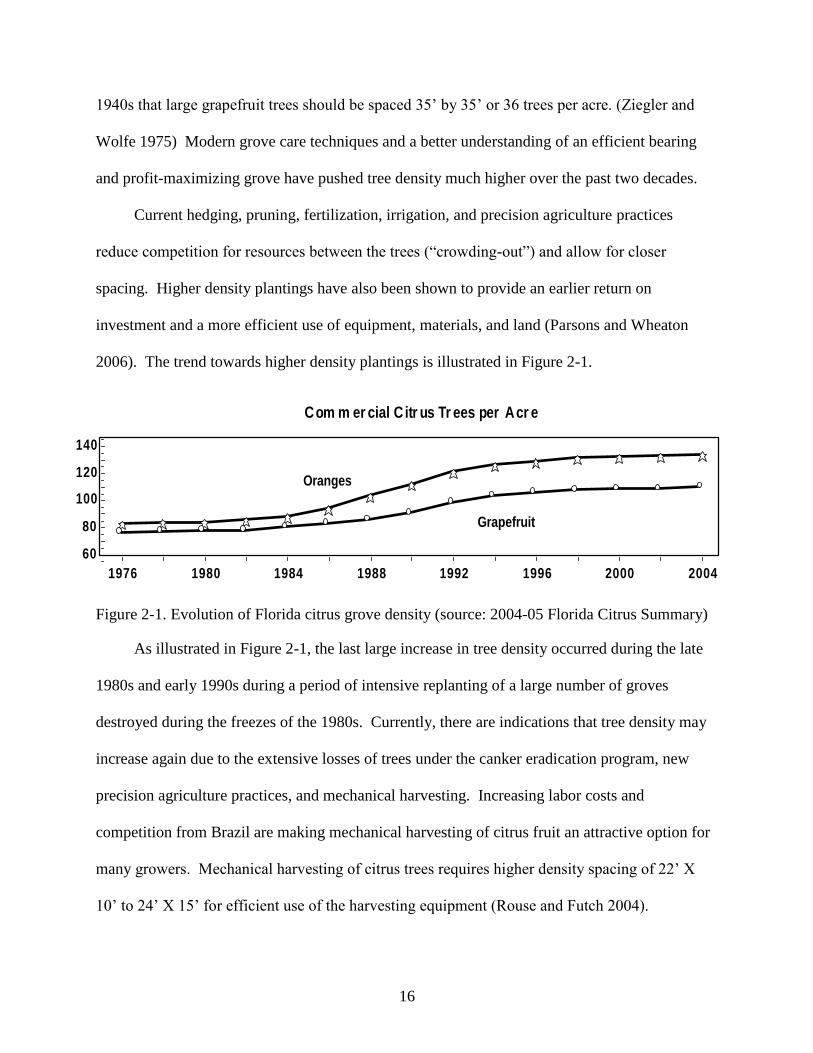
Current hedging, pruning, fertilization, irrigation, and precision agriculture practices
reduce competition for resources between the trees (“crowding-out”) and allow for closer
spacing. Higher density plantings have also been shown to provide an earlier return on
investment and a more efficient use of equipment, materials, and land (Parsons and Wheaton
2006). The trend towards higher density plantings is illustrated in Figure 2-1.
Figure 2-1. Evolution of Florida citrus grove density (source: 2004-05 Florida Citrus Summary)
As illustrated in Figure 2-1, the last large increase in tree density occurred during the late
1980s and early 1990s during a period of intensive replanting of a large number of groves
destroyed during the freezes of the 1980s. Currently, there are indications that tree density may
increase again due to the extensive losses of trees under the canker eradication program, new
precision agriculture practices, and mechanical harvesting. Increasing labor costs and
competition from Brazil are making mechanical harvesting of citrus fruit an attractive option for
many growers. Mechanical harvesting of citrus trees requires higher density spacing of 22’ X
10’ to 24’ X 15’ for efficient use of the harvesting equipment (Rouse and Futch 2004).
1976 1980 1984 1988 1992 1996 2000 2004
60
80
100
120
140
Com m er cial C itr us Tr ees per Acr e
Oranges
Grapefruit
17
In this analysis, new planting densities are assumed to be 198 trees per acre (22’ by 10’
spacing) for Valencia and Hamlin varieties, and 134 trees per acre (22’ by 13’) for grapefruit.
Mature groves tree densities are taken from the 2003-4 IFAS Citrus Production Budgets as
common densities for existing groves (Muraro 2005 I, II, III). Mature grove densities are
assumed to be 112 trees per acre for Valencia and Hamlin on the Ridge, 145 trees per acre for
Valencia and Hamlin on the Flatwoods, and 95 trees per acre for grapefruit.
In the case of a new or replanting of citrus, this analysis uses an irrigation installation and
setup cost of $1000 per acre for the ridge and flatwoods production areas. New plantings may
require a well to be drilled, which increases the cost of installation, but this is not included in the
analysis. A replanted grove is assumed to incur the same cost for irrigation installation due to
two observed practices (Muraro and Futch 2006). First, the irrigation system is usually damaged
during the process of removing (“pushing”) the previous grove. Second, a new system layout is
usually required, especially if there are changes to tree density or other grove architecture.
This analysis does not include the costs of removing or pushing the previous grove, and
starts with the assumption that the land is vacant. Preparing open land for citrus varies
substantially by topographic area (ridge versus flatwoods). Flatwoods groves incur higher land
preparation costs compared to ridge groves. Changes to grove architecture and/or tree density
require incurring costs for soil preparation and bed construction all over again. Therefore, this
analysis assumes that new plantings and replantings of citrus will incur the same land preparation
costs. Average citrus land preparation costs used in this analysis are summarized in Appendix
Table B-10.
Grove Care and Operating Cost Considerations
Citrus fruit is utilized either in the fresh processed market, and in both cases must be
transported from the tree to the juice processing plant or fresh fruit packing house. This process
18
is currently accomplished in three steps: picking the fruit off the tree, roadsiding it by
transporting it from inside the grove to a central loading point, where the fruit is then hauled to
its final destination. These costs are influenced by wage rates, equipment/materials costs, and
fuel/energy costs. These unit costs are substantial, usually are incurred on a per box basis, and
may exceed grove care costs.
Harvesting costs have remained somewhat stable over the past decade, and this enables the
grower to project how much it will cost with some certainty. Wage rates, fuel/energy costs (until
recently), and equipment/materials costs have remained stable. Unfortunately, there are
uncertainties in the supply of agricultural labor, especially for groves located outside of the
major Florida production areas and for late season varieties such as Valencia oranges. Grapefruit
prices in this analysis are quoted as the industry-standard “on-tree” price meaning the price for
pick, roadside, and haul is already subtracted and they do not include a harvesting charge.
Orange prices are “delivered-in” to the processing plant, and include a per box harvesting charge.
This analysis uses average reported costs from the 2004-05 season of $1.64/box for picking and
roadsiding, and $.47/box for transporting the fruit to the juice processing plant for a total of
$2.11 (Muraro 2006 II). Details of individual per box costs can be found in Appendix Table B7.
Additionally, the Florida Department of Citrus (“DOC”) collects a per box excise tax to
fund citrus marketing and industry research. While there have been several legal challenges to
the box tax, plus a current proposal to raise the box tax to $0.25, this analysis assumes a rate of
$0.185 per box, giving a total per box cost of $2.30.
Due to the special handling requirements for fresh fruit, an extra charge of $1.50 per box is
assumed for citrus fruit to be marketed as fresh. Additional handling can include special
packaging and transportation from the grove to ensure the visual appeal of the fruit. Moreover,
19
spot picking is a common practice in fresh fruit groves, where pickers identify and ensure only
the highest quality fruit is picked and sent for sale as fresh. The assumed pick and haul cost for
fresh market fruit is $3.80 per box.
For most growers, agricultural chemical and application costs are the largest production
cost after harvest costs. The diverse uses of agricultural chemicals in citrus for pest control,
disease control, growth regulation, and nutritional supplementation blur the classifications of
fixed-variable costs and range from certain to uncertain. It is the difficult task of the citrus
grower to balance the health and productivity of his/her trees while minimizing the cost of
materials used. In practice, this is a subjective judgment based on the individual experience of
the grower as illustrated by a 2001 survey of spray practices in the Indian River region.
Research and extension literature on citrus spraying rightly focuses on the
complexity of predicting effects of spray practices on distribution of materials
within trees, even in controlled experiments. Consequently, recommendations from
authorities often provide limited guidance to growers. This forces the industry to
explore spraying as an art, in which changes are attempted on an ad-hoc basis and
either rejected or continued based on individual experience or reports from peers.
The tremendous range of grower spray practices appears to reflect the current status
of this ongoing, largely independent, experimentation by individual growers
(Stover et al. 2002a).
There are significant differences in spray costs for citrus fruit grown to be consumed fresh,
and fruit grown for processing into juice. Fresh market fruit requires a blemish-free peel to
enhance its marketability and visual appeal to the consumer. Fresh fruit is delivered to a
packinghouse where it is sorted according to size and peel blemishes. The fruit judged unfit for
fresh consumption is “eliminated” from the total amount delivered, and sent for processing into
juice. The percentage of the total fruit delivered to the packinghouse that is fit for fresh market
sale is called the “packout” rate. Often a fresh fruit packinghouse will deduct a fee for the
eliminated fruit that passes through its packing line and is transported to a juice processing
facility. This fee is deducted (or “charged”) from the total payment to the grower. Fruit sent for
20
processing generally receives a significantly lower price than fresh. Therefore, it is imperative
that a grower obtains a high packout rate to maximize the amount of his production receiving the
highest price, and minimize the possibility of receiving a lower price for eliminations. This is
mostly accomplished through the spray program and spot picking practices as described in the
previous section.
Fungal diseases and insect damage are the two most common causes of peel blemishes and
reasons for fruit elimination. Fungal infections, such as melanose, citrus scab, alternaria, and
greasy spot, are often controlled using fungicidal sprays containing copper and petroleum oil.
Some insects, commonly mites, attack the fruit/peel and must be controlled using pesticides to
ensure fresh market quality.
Citrus trees are attacked by a number of foliar and root pests and diseases that affect
productivity. When balancing lost productivity with the costs of chemical application, the use of
chemical control is generally required when a certain level of infestation or infection is reached.
Fruit grown for the processing market does not require high external quality. In this case, spray
costs appear to be closer to a variable cost of production which increases with yield.
In Florida, most sweet orange varieties, with the exception of Navel oranges, are grown for
the processing market (Table 2.1). Grapefruit, tangerines, and other specialty varieties are
mostly grown for the fresh market. Due to the factors discussed above, spray costs for the fresh
market varieties are significantly higher than oranges for processing. For example, Table 2.2
illustrates the difference in spray costs between the Hamlin orange variety and the red-seedless
grapefruit, grown for the processed and fresh markets respectively. The reader should note that
these spray programs include micronutrient compounds that are mixed into a solution containing
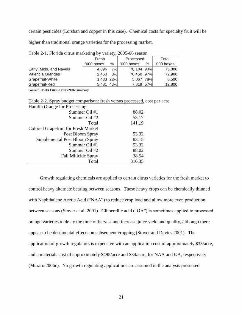
21
certain pesticides (Lorsban and copper in this case). Chemical costs for specialty fruit will be
higher than traditional orange varieties for the processing market.
Table 2-1. Florida citrus marketing by variety, 2005-06 season
Fresh Processed Total
'000 boxes % '000 boxes % '000 boxes
Early, Mids, and Navels 4,896 7% 70,104 93% 75,000
Valencia Oranges 2,450 3% 70,450 97% 72,900
Grapefruit-White 1,433 22% 5,067 78% 6,500
Grapefruit-Red 5,481 43% 7,319 57% 12,800
Source: USDA Citrus Fruits 2006 Summary
Table 2-2. Spray budget comparison: fresh versus processed, cost per acre
Hamlin Orange for Processing
Summer Oil #1 88.02
Summer Oil #2 53.17
Total 141.19
Colored Grapefruit for Fresh Market
Post Bloom Spray 53.32
Supplemental Post Bloom Spray 83.15
Summer Oil #1 53.32
Summer Oil #2 88.02
Fall Miticide Spray 38.54
Total 316.35
Growth regulating chemicals are applied to certain citrus varieties for the fresh market to
control heavy alternate bearing between seasons. These heavy crops can be chemically thinned
with Naphthalene Acetic Acid (“NAA”) to reduce crop load and allow more even production
between seasons (Stover et al. 2001). Gibberellic acid (“GA”) is sometimes applied to processed
orange varieties to delay the time of harvest and increase juice yield and quality, although there
appear to be detrimental effects on subsequent cropping (Stover and Davies 2001). The
application of growth regulators is expensive with an application cost of approximately $35/acre,
and a materials cost of approximately $495/acre and $34/acre, for NAA and GA, respectively
(Muraro 2006c). No growth regulating applications are assumed in the analysis presented
22
because of the focus on oranges and grapefruit varieties, however for certain, primarily fresh
market citrus varieties, incorporation of these costs is an important component of analysis.
Intuitively, older trees with large canopy volumes should require more amounts of
chemicals, however, there is considerable variability between large tree size, high spray volume,
and increased chemical costs. A 2001 UF-IFAS survey of spraying practices in the Indian River
growing region reported some association between spraying large trees at a high spray volume,
but some growers also reported spraying small trees at a high volume (Stover et al. 2002b). Due
to the high cost of chemicals and the economics of spray efficiency, Florida citrus has moved
quickly to adopt variable rate sprayers that can adjust the amount of chemical material applied to
the tree size. Overall, chemical control for pests and disease requires more spray material to
cover increased canopy size as trees age; however, spray costs and materials for young, small,
and/or non-bearing trees will differ as explained in a following section on young tree care. This
analysis assumes that the grove manager or caretaker uses variable rate spraying equipment
methods to apply the quantity of spray material appropriate for the tree age. These costs are
adjusted according to age as shown in Appendix Table B-8.
A productive citrus grove must maintain a certain level of upkeep during its operation. In
the hot and humid Florida environment, other plant species quickly invade a grove and compete
with citrus trees for water, sunlight, and soil nutrients. Cultivation includes controlling for these
uninvited plants through mechanical mowing and herbicide applications. Labor for general
maintenance and upkeep is required to perform a multitude of necessary tasks around the grove.
While these costs may vary significantly, a grower is certain that they will be incurred.
Estimates of cultivation and grove maintenance costs for the 2005-06 season ranged from $80 to
$100 per acre depending on the grove’s location in the state.
23
The generic term “pruning” generally involves three components in a citrus grove:
pruning, hedging, and topping. Pruning refers to removing selected limbs to alter the structure of
the tree in order to reduce overcrowding between trees in a row. Crowding has a negative effect
on yield, juice, and peel quality. Hedging refers to cutting back the trees from encroaching on
the space between the rows (row middles), and allowing grove equipment to pass through.
Topping refers to cutting the top off the tree to prevent it from being excessively tall. Topping
facilitates harvesting, reduces the amount of spray materials needed, and avoids the shading-out
of other trees (Parson and Wheaton 2006).
The frequency of pruning, hedging, and topping depends on the planting density and
vigorousness of the citrus variety and rootstock. Planting the trees in a tighter spacing will
necessitate more frequent pruning to avoid overcrowding. Accordingly, trees planted on
vigorous rootstocks such as Rough Lemon or Volkameriana will encroach on each other faster
than Swingle or Cleopatra rootstocks. A grapefruit tree will encroach faster than a Valencia
orange tree. The 2004-05 IFAS Citrus Budget reports annualized total costs ranging from $28 to
$44 per acre depending on variety and location. This analysis assumes the pruning costs to be
incurred from the fourth year of tree age onwards.
An adequate citrus fertilization program is essential to cultivating productive and healthy
trees. The fertilization of citrus trees increases yields, growth, and has been shown to aid tree
recovery from damage due to weather, disease, or pests (Morgan and Hanlon 2006). Citrus trees
require a large amount of macronutrients (nitrogen-N, phosphorous-P, and potassium-K), and
smaller amounts of micronutrients (iron-Fe, zinc-Zn, manganese-Mn, boron-B, molybdenum-
Mo, and others). Of these nutrients, nitrogen is the most important and is frequently applied in
the form of solid fertilizer through multiple soil applications per year (Zekri and Obreza 2003).
24
Micronutrients are applied as foliar sprays, can be combined with other chemical sprays, and are
usually applied as needed when trees exhibit symptoms of micronutrient deficiency.
An individual grove’s fertilizer program may vary by soil type, tree age, variety, and
specific grove conditions. Moreover, some growers are now using fertigation techniques where
macronutrients are applied in a liquid form through the irrigation system. A typical fertilization
schedule for oranges requires three annual applications by mechanized fertilizer spreaders of
about 210 pounds per acre with grapefruit requiring about three-quarters (150 pounds) of that
amount (Jackson and Davies 1999). IFAS estimates for show for the 2005-06 season a range of
$50 to $70 per application per acre. This analysis assumes a cost of $205 per acre per year for
oranges, and $157 per acre per year for grapefruit. This analysis does not make an allowance for
micronutrient sprays.
Most Florida soils used for citrus production are acidic with a low pH in their native state
and require infrequent applications of soil amendments to raise their pH. Citrus trees grow best
in a pH range of 6.0 to 6.5, and pH values outside of this range affect the absorption of nutrients
by the tree and may reduce tree productivity and growth (Obreza and Collins 2002). The most
commonly applied amendment to raise soil pH is Dolomite limestone, and this is applied as
necessary by the pH level of the soil. Soil and drainage characteristics of the grove determine
the behavior of soil pH, but for the purposes of this analysis, one ton per acre is assumed to be
applied once every three years for an annualized cost of $13.97.
Horticultural and economic considerations require most commercial citrus in Florida to be
irrigated. Many Florida citrus trees are planted on porous and sandy soils that do not retain
sufficient moisture for the tree all year. A citrus tree becomes drought-stressed if it does not
receive enough water, and this has a negative effect on yields, juice quality, and fruit size (Mongi
25
et al. 2003). Moreover, irrigation can effectively be used for cold protection during freeze
events, especially for vulnerable young trees (Parsons and Bohman 2006). Finally, irrigation
reduces yield uncertainty and mitigates risk of financial difficulty due to crop failure caused by
drought.
Several different irrigation systems exist and require different components and designs, but
microsprinkler and micro-jet irrigation have become widely adopted by Florida commercial
citrus. This analysis assumes the use of a microsprinkler irrigation system and is comparable in
costs to a micro-jet system. Costs for operating a microsprinkler irrigation system vary by
location due to additional costs for water management in Flatwoods groves.
In the Florida citrus industry, the process of removing a dead or unproductive tree and
replacing it with a new nursery tree is commonly called “resetting”, and the tree itself is called a
“reset”. Pests, diseases, freezes, lightning, and many other unpredictable and sometimes
unexplainable factors claim the lives of citrus trees. Resetting is an important part of
maintaining a citrus grove at maximum bearing efficiency with a full complement of healthy
trees. The publicly available Florida Commercial Citrus Tree Inventory is conducted every two
years by the FASS, since 1966. Change in commercial citrus acreage is determined by aerial
photography, that identifies the number of existing trees by variety and year planted. The
average tree loss by age group used for this analysis is 1% for trees aged 1-3 years, 1.5% for
trees aged 4-11 years, and 3% for trees 12+ years of age.1
1 This analysis uses an unpublished analysis conducted by Dr. Mark Brown of the Florida Department of Citrus
which compared the changes in the tree inventories by tree age from 1994 to 2004, interpolating for between survey
years. After subtracting for non-bearing trees to eliminate for newly planted trees and for canker eradications, a
linear regression line was fit to account for the increase in losses as trees age. Unfortunately, this data may include
some citrus acreage lost to non-agricultural development, and overestimate the actual tree loss suffered in a healthy
grove; however, interviews of grove managers conducted by the author confirm that these loss rates are reasonable.
26
Resetting a new tree in a mature grove requires incurring immediate and continuous costs
for up to three years. In the near term, the dead/unproductive tree must be removed and the new
tree purchased and planted. This involves additional labor, materials, and equipment time to pull
out the dead tree and dispose of it, clear weeds, aerate the soil, apply a soil fumigant, and plant
the new tree (Jackson 1994). In the longer term, the newly planted tree requires additional care
such as, removing unwanted sprouting, weed control, special fertilization and irrigation
programs, and the maintenance of cold-insulating tree wraps. See Appendix B for detailed cost
information.
Given the costs involved and the delay for reset trees to come into production, growers
attempt to optimize their resetting strategy for maximum economic gain. Nursery trees are
usually ordered one or two years in advance, and special equipment and labor must be arranged
for planting. IFAS Extension publishes an on-line decision aid for optimal resetting strategy that
includes costs, yields, prices, and loss rates (Roka et al. 2000). It is suggested that in high
density and new plantings, a program of continuously resetting dead/unproductive trees may
increase returns to investment; however, IFAS Citrus Economist Ronald Muraro observes that,
under field conditions, most growers only reset trees every other year (biennial resetting) or
longer (Muraro 2006d).
In addition to grove care expenses, there are general operating expenses which must be
considered. Growers may have fixed costs for buildings, equipment, and other costs that cannot
be allocated just to a single grove or on a per acre basis. Since these costs are highly dependent
on a grower’s individual situation, this analysis attempts to limit the number of assumptions
made about a grower’s fixed expenses. A per acre cash cost is assumed that captures typical
fixed expenses such as equipment use, structures, and grove administration by charging a
27
management fee. Property taxes are included on a per acre basis, and a “miscellaneous” cost that
accounts for tools, repairs, and additional grove labor.
Citrus production management in Florida is a highly diverse field, with many grove
caretaking tasks being contracted to third-party caretakers. The spectrum runs from grove
owners who own production equipment (tractors, sprayers, harvesting equipment, etc.) and hire
employees, to owners who contract all production work, including harvesting, for a set fee or
percentage of revenue. IFAS citrus production budgets designate the former as an “owner-
managed” operation, and the latter as a “custom-managed” operation. In the custom-managed
production costs, IFAS citrus production budgets incorporate a 10% surcharge on materials cost
(chemicals and fertilizer), and use “custom” rates reported by grove caretakers and managers.
Many growers fall in between these two extremes, and own some grove equipment, perform
some production work themselves, contract for other work, or perform contract work themselves.
In this analysis, costs are reported for an owner-managed operation. Figures given for
spray and fertilizer materials costs are reduced by 10% from reported IFAS citrus production
budgets. All other grove care costs reflect an owner-managed operation with equipment
depreciation incorporated into the costs. A 5% “management” charge is applied to account for
other fixed and indirect expenses not directly incorporated into the grove care costs.
Property tax on Florida agricultural land is known as the millage rate, and is calculated on
a per $1000 of assessed value basis. Reported millage rates range from a low of 11.5 per $1000
of assessed value (1.15% per year) in Collier County to a high of 29.6 per $1000 (2.96% per
year) in Pinellas County. Millage rates for the top four citrus producing counties are illustrated
in Appendix B - Table B-11 (Hodges et al. 2003).
28
The land value used for property tax assessment (the assessed value) of agricultural
enterprises will usually be lower than the market (just) land value. The tax-assessed value is
based on the value of the land derived from the returns to agricultural use. The procedure used
to assess agricultural value differs by county and the tax assessed land value varies widely. In
this analysis, an average millage rate of 19.5 (1.95%/year) is assumed, with an assessed value of
$3,600 per acre for a mature grove, and $1,550 per acre for a new planting or replanting which
results in about $70 per year and $30 per year in property taxes, respectively. The values were
put into 2003 figures because that is the last publication available with all country agricultural
property tax rates collected (Hodges et al. 2003). The just value given for a mature grove and a
new/replanted grove is taken from the 2003 IFAS Florida Rural Land Value Survey (Reynolds
2003). The dollar amount of property tax is assumed to increase by 2.5% per year over the 15-
year period of analysis reflecting natural growth in the value of agricultural and basic inflation.
A miscellaneous cost of 2% of grove care expenses is added to account for general grove
labor and materials. In the base scenario, this cost varies from $14.65 per acre for oranges on the
ridge to $19.80 per acre for grapefruit on the flatwoods. This is based on the observation that
there are many indirect costs and expenses incurred in grove management for additional labor,
tools, and materials.
Cash outflows (expenses) to pay for the previously described expenses are incurred
throughout the year. Citrus trees in Florida produce one crop per year that generates a cash
inflow (revenue). Many different payment schemes exist where growers contract for delivery of
the fruit and receive a portion of the total payment before delivery. One method to value the
timing mismatch between cash inflows and outflows due to operations is referred to as working
29
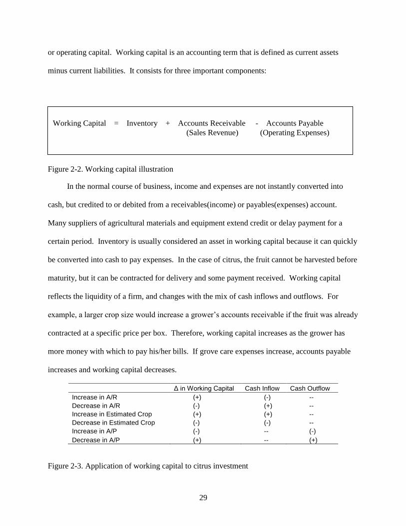
or operating capital. Working capital is an accounting term that is defined as current assets
minus current liabilities. It consists for three important components:
Figure 2-2. Working capital illustration
In the normal course of business, income and expenses are not instantly converted into
cash, but credited to or debited from a receivables(income) or payables(expenses) account.
Many suppliers of agricultural materials and equipment extend credit or delay payment for a
certain period. Inventory is usually considered an asset in working capital because it can quickly
be converted into cash to pay expenses. In the case of citrus, the fruit cannot be harvested before
maturity, but it can be contracted for delivery and some payment received. Working capital
reflects the liquidity of a firm, and changes with the mix of cash inflows and outflows. For
example, a larger crop size would increase a grower’s accounts receivable if the fruit was already
contracted at a specific price per box. Therefore, working capital increases as the grower has
more money with which to pay his/her bills. If grove care expenses increase, accounts payable
increases and working capital decreases.
Δ in Working Capital Cash Inflow Cash Outflow
Increase in A/R (+) (-) --
Decrease in A/R (-) (+) --
Increase in Estimated Crop (+) (+) --
Decrease in Estimated Crop (-) (-) --
Increase in A/P (-) -- (-)
Decrease in A/P (+) -- (+)
Figure 2-3. Application of working capital to citrus investment
Working Capital = Inventory + Accounts Receivable - Accounts Payable
(Sales Revenue) (Operating Expenses)
30
Although the actual cost of maintaining working capital throughout the season varies
significantly by grower circumstance, in this analysis an interest charge of 6% on operating
expenses is incurred for a period six months out of each year of analysis. This is assumed to
account for the costs of maintaining sufficient working capital for production of that year’s crop.
Tree Yields
Yield expectations per tree in generalized Florida growing conditions are summarized from
published data. The Florida Agricultural Statistics Service (FASS) division of the USDA has
calculated average yield by tree age, variety, and region of Florida (Indian River, North &
Central, West, and South) since 1993. The USDA derives the average yield per tree by using the
Commercial Citrus Inventory’s record of trees by age and end-of-season field samples of
production per tree by age (Florida Agricultural Statistics 2006). Appendix Table B13
summarizes the FASS data by tree age and region. At the time of writing, the state average
yields by tree age over the 2000-2005 period are available, but were not used because they are
lower than previous periods due to the effects of the 2004-5 Atlantic Hurricane Season,
especially for the Indian River and Western regions. Since 1960, the Savage yield-tree age study
was frequently used by growers to benchmark their own grove’s results (Savage 1960). The
Savage study may no longer be applicable due to its limitation to ridge groves and low-density
plantings (48 to 70 trees per acre). More recent studies by the researchers at the University of
Florida-IFAS track box and juice yield by tree age in higher density plantings at both ridge and
flatwoods sites. A study of Valencia oranges on twelve rootstocks by Dr. William Castle tracks
box and juice yields by tree age over a 15 year period in both ridge (Avon Park) and flatwoods
(Indiantown) locations (details in Appendix Table B14, Castle 1994). The findings indicate a
trend in high-density plantings in that production per acre reaches a maximum and plateaus
31
earlier, around year 10 or 11 of tree age, than trees with wider spacing. This is due to trees
competing with each other for sunlight, water, and nutrients (Parsons and Wheaton 2006).
Fortunately, the reduced per tree yield is compensated by a greater number of trees for
comparatively more production per acre.
Another study of high density (150+ trees per acre) flatwoods plantings at theUF/IFAS
Southwest Florida REC examined Valencia and Hamlin oranges primarily on Carrizo and
Swingle rootstocks and confirms the plateau of box yields around 8 to 10 years of age.
Moreover, a comparison of the Valencia and Hamlin orange varieties shows that Hamlins
produce between 100 and 120 boxes per acre more than Valencias. (Roka et al. 2000).
Additionally, while Hamlins produce less pounds-solid per box, Hamlins annually out produce
Valencias by 200 to 800 pounds-solid per acre.2
Pounds-solid per box varies due to various biological and environmental factors, and also
depends on variety and rootstock. In addition to the quantity of pounds-solid per box, the quality
of juice is important. Juice with a good color and a sufficiently high sugar to acid ratio (Brix
ratio) receives a premium from juice processors. Late-season Valencia oranges usually exhibit
better juice quality than early-season Hamlins, and the price per pound-solid for Valencias are
generally higher than the price paid for Hamlins (Spreen et al. 2001). Varieties grafted to
rootstocks such as Carrizo, Sour Orange, and Swingle tend to give higher pounds-solid than
2 Pounds-solid is very important for oranges sold for juice processing because growers are paid on the basis
of the pounds-solid measure of juice quantity and not the number of boxes. While a box of oranges always weighs
90lbs, the quantity and quality of juice that can be squeezed from the fruit varies. Orange juice contains water,
sugar, and a diverse range of other organic molecules. Sugars constitute about 75% of the dissolved solids in orange
juice, and are directly proportional to the quality of the juice. The density of the dissolved solids in the orange juice
is measured in degrees Brix, named after the German scientist who discovered how to measure this relationship.
Degrees Brix is converted into the percentage of soluble solids in the juice and multiplied by the amount of juice
squeezed per box to arrive at the number of pounds of solids (abbreviated to pounds-solid or p.s.) per box of
oranges.
32
Rough Lemon and Volkameriana (Jackson and Davies 1999, Castle 1994). When interpreting
the results of this analysis, it is important to remember these differences in breakeven prices.
The preceding sources were used to construct an average box and pounds-solid yield per
tree by age for this analysis. Differences in topography, soil, climatic conditions, and grove care
all play a role in the yields of a particular grove; however these yields are assumed to control for
random effects and represent what a grower can expect from a healthy, well-managed tree.
Therefore, the above information was adjusted with the opinion of IFAS experts to reflect the
expected average yield of a typical Florida grove using standard grove care techniques (Muraro
2006d). Unfortunately, no detailed studies of grapefruit yields exist; instead an approximation of
the state average yields for colored grapefruit is used and adjusted for higher densities. Pounds-
solid are not calculated for grapefruit because it is assumed that grapefruit is produced for the
fresh market. The analysis yields also incorporate a resetting effect due to the resetting of only
half of the total tress lost after year 10 of grove age, which makes more space available for each
tree. The maximum yield in year 10 was increased by 10% for years 11-15 due to trees growing
out into the wider spacing.
33
CHAPTER 3
ACCOUNTING FOR THE EFFECTS OF CITRUS CANKER AND GREENING ON
FLORIDA COMMERCIAL CITRUS PRODUCTION
The Florida citrus industry currently faces two new disease challenges with unpredictable
consequences. Citrus canker is a bacterial disease of citrus that causes unsightly lesions on citrus
leaves and affects tree productivity. Citrus greening, or Huanglongbing (HLB), is a bacterial
disease of citrus that quickly kills trees. Both diseases are highly contagious and have the
possibility of spreading rapidly through commercial production areas of the state. Under the
canker eradication program, any tree detected with citrus canker was required to be eradicated,
along with all other trees within a 1900-foot radius. Growers were compensated by the USDA-
Animal and Plant Health Inspection Service (APHIS). This program was halted in January 2006,
and the management of canker is now the responsibility of individual growers. In August of
2005, citrus greening was first detected in a residential citrus tree near Homestead in Dade
County, and has spread to all of other citrus producing counties. The Florida Department of
Agriculture and Consumer Services (FDACS) made it known that there will not be a greening
eradication program. Florida commercial citrus production is entering an environment of
endemic citrus canker and greening. Due to the novel nature of these challenges to citrus
production, this analysis surveys current academic literature on these diseases in order to
describe their grove-level effects on citrus.
Citrus Canker
Canker bacteria are spread by windblown rain, human and mechanical contact. It enters
the citrus tree through natural openings and wounds in the protective outer tissue of the trees, and
is exacerbated by the citrus leafminer insect. Depending on weather conditions, canker
symptoms appear from about a week to a couple months after infection, and are especially
virulent in hot and humid weather. Severe infections may cause defoliation, badly blemished
34
fruit, premature fruit drop, and tree decline (Schubert and Sun 2001). Studies suggest that the
canker bacteria can be spread over two miles from normal wind and rain alone, with longer
distances of 10 miles and greater possible due to hurricanes and other severe weather events
(Gottwald et al. 2002a).
Florida’s first experience with citrus canker was an outbreak around 1910 that was not
eradicated until 1933. Canker is hypothesized to have arrived in Florida on plant material
imported from Japan (Gottwald et al. 2002 II). After 53 years, canker reappeared in Manatee
county in 1986, and after an extensive eradication program, it was declared eradicated in 1994.
The next year, canker reappeared in a residential citrus tree near Miami airport, and was the
focus of the most recent eradication program. From 1995 onwards, citrus canker was subject to
an eradication program which until 1999 destroyed all trees within a 125 ft. radius of an infected
tree. In 1999, a new study showed that canker was spread much farther than previously thought,
and a 1900 ft. radius of eradication was mandated, plus any cleared land was required to be left
fallow for 2 years. The “1900 ft. rule” was statistically determined to eliminate 99% of the
bacteria spread within 30 days. According to a USDA study, Hurricane Wilma in 2005 may
have exposed 168,000 to 220,000 acres of commercial citrus to canker, in addition to the 80,000
acres already exposed by the 2004 Hurricanes Charley, Francis, and Jeanne (FDACS 2000a).
Approximately 7.5 million commercial trees, 860,000 residential trees, and 4.3 million
nursery trees were eradicated from 1995 until the end of the program. Canker finds are now
reported in all of the top twelve citrus producing counties. (FDACS 2006 II) With the halt of
the citrus canker eradication program, canker will now likely become endemic to Florida for the
first time in the history of the industry.
35
The effects of canker in a citrus grove depend on the susceptibility and market outlet of the
fruit. White and colored grapefruit, Persian (Tahiti) limes, and early and midseason oranges
(especially Navel and Hamlin varieties) are the most susceptible citrus varieties. Valencia
oranges, tangelos, and tangerines appear to be less susceptible to canker (Gottwald et al. 2002b).
Canker does not affect the juice quality of fruit, but the unsightly canker peel blemishes and
quarantines against fresh fruit shipments from canker infected areas lead to the conclusion that
the profitability of fresh market citrus will be impacted more severely than citrus for juice
processing. Studies of citrus production in certain areas of Brazil and Argentina where canker is
endemic suggest guidelines for specific integrated management programs for the control of
canker in a grove (Leite and Mohan 1990, Spreen et al. 2001a, Muraro et al. 2001).
Tree Loss and Yield Reduction Due to Canker
Canker has not been conclusively shown to kill trees in the short and medium term, but a
severely infected tree may become unproductive, and serves as a source of inoculum (bacteria)
that can be spread to neighboring trees. An integrated management program includes removal of
infected trees and some neighboring ones. This analysis assumes an increase of 10% in
historical tree loss rates for all age categories.
The hurricane seasons of 2004 and 2005 not only spread canker through commercial
groves but affected large numbers of citrus tree nurseries. As of 2004, 70% of Florida citrus
nurseries were “field” nurseries where trees are grown outdoors, and are vulnerable to wind and
rain spread canker. Canker eradication destroyed nearly two-thirds of the existing nursery tree
inventory, and eliminated important sources of budwood for propagating new trees (Spreen et al.
2006). Few nursery trees were available for the next two years, with limited production for the
36
next three to five years. This analysis uses a figure of $7.50 per tree to account for increased
price due to decreased supply during the next 2-5 years.
Susceptibility and canker’s resulting damage to a tree varies by citrus variety. Infected
trees exhibit twig dieback and leaf, flower, and fruit drop (Gottwald 2006 II). Hamlin oranges
and grapefruit are considered highly susceptible, and information from Argentina’s experience
with endemic canker indicates possible yield losses of 10-20% for highly susceptible varieties
(Spreen 2001). This analysis assumes a yield penalty of 10% for Hamlin oranges and grapefruit.
Valencia oranges are considered moderately susceptible, and are assessed a lower yield penalty
of 5%.
Canker Management: Augmented Spray Programs
Canker increases the cost of spray programs for the most susceptible varieties, especially
grapefruit for the fresh market. Studies show that copper sprays reduce the canker inoculum
(bacteria) build up on the leaf and fruit surfaces of infected trees, with 3-5 annual sprays for
moderately susceptible varieties and 4-6 for highly susceptible varieties (Gottwald 2006b). The
citrus leafminer insect is currently under somewhat successful biological control, and also is
controlled for by oil-based spray applications (Heppner 2003).
For the purposes of this analysis, it is necessary to determine the additional spray material
and application costs canker adds to standard spray programs. Copper spray is already widely
used as a fungicide/bactericide in Florida to control for melanose, greasy spot, and scab,
especially for the fresh market (McCoy et al. 2005). Petroleum-based oil sprays are also used
extensively to control for insects such as scales, and other diseases. Many of these sprays can be
mixed together, and applied at the same time. Upon consultation with IFAS Lake Alfred CREC
experts, additional spray applications, schedules, and costs were determined for canker control
37
(see Appendix Table B-17). Valencia and Hamlin oranges for the processed market, and
grapefruit annual spray costs are expected to increase $20.96, $48.17, and $35.26 per acre,
respectively.
Canker Management: Field Inspections
Aggressive field inspections and decontamination of workers and grove equipment to
identify canker sources and control its spread are a vital part of the canker management program.
Three yearly field inspections by trained personnel were estimated at $5.84/acre/inspection
(Muraro 2006d). This cost was calculated for a 120-acre grove, using nine inspectors and two
vehicles, and may vary depending on the size and location of the grove.
Canker Management: Windbreaks
Windbreaks are densely planted stands of large trees not susceptible to citrus canker
planted along the borders of a grove or block of citrus. The intent is that the protection of the
trees will stop or deflect the spread of windblown canker for outside sources. This has proved
successful in Argentina and Brazil for protecting groves, and is a likely part of an integrated
canker management program, especially for fresh market fruit (Leite and Mohan 1990). The
annual cost used in this analysis for establishing and maintaining a windbreak is estimated to be
$11.47/acre for a 10-acre block over 20 years, and in this analysis is only included for grapefruit.
There may be additional costs due to lost production from the reduction in grove area planted in
citrus and the shading out of existing trees that are not included in this analysis (see Appendix
Table B15 for a detailed breakdown of costs and additional information).
Canker Management: Packinghouse and Export Certification for Fresh Market Citrus
Fresh fruit must be handled in designated packinghouses where fruit is treated with
disinfectants, and some processing plants and packinghouses refuse to accept fruit from infected
38
groves. In the future endemic canker environment, packinghouses are expected to pass along the
cost of special handling to growers. This analysis assumes $.10 per box (or $40.50/acre @ 450
boxes/acre) based on conversations with industry professionals and academics. Moreover, it is
likely that the DPI will require special inspections for groves exporting internationally, and this
cost is estimated at $60/acre. In the analysis, these costs are only incurred for fresh market
grapefruit after the trees become commercially harvestable at three years of tree age.
Citrus Greening
Citrus greening or Huanglongbin (HLB) is a bacterial disease of citrus native to Asia.
Greening (bacteria species name: Candidatus Liberibacter) gets its name from the small, green
fruit produced by an infected tree. Infection causes the quick decline and death of a tree in about
two to four years. After its initial detection in August of 2005 in Homestead, greening has
spread throughout the state. Greening is spread by an insect vector named the Asian citrus
psyllid which is widely distributed throughout the state and is difficult to control. The exotic
nature of greening in Florida and lack of a definitive management program means there is very
little information about the effects of greening on the production and costs of a grove. Greening
has devastated the citrus industries of other countries, but little is known about how greening will
behave in the intensive grove management environment of Florida. Most existing literature on
greening is found in scientific journals specializing in virology or plant pathology. As of this
writing, there exist only two studies of the economic impact of greening (Grezebach 1994,
Roistacher 1996), and both study greening’s effect on the Thai citrus industry. Other countries’
experiences with greening serves as the basis for the assumptions reached below, and may not
reflect the realities of greening in Florida.

39
Literature Survey of International Experiences with Greening
In Taiwan, greening was first discovered in 1951 with significant spread by 1970’s. Its
transmission was spread by propagation with infected material and the psyllid vector. In a field
study with .78 Ha (240 tangerine trees) in a greening endemic area with no control, psyllid
infestation was found five months after planting, with 89% of trees infected within eight months
after the infestation was discovered (Chen 1998). Trees expressed symptoms of greening and
dieback approximately two and one-half years after the initial infection.
A greening-like disease (CVPD) was first discovered in Indonesia in the 1950s, and was
present in most major production areas by a 1984 survey (Vichtranada 1998). With an integrated
pest management program (IPM), yields increased 200% in certain areas.
A Vietnamese survey conducted in 1995 found greening in all citrus production areas of
Vietnam, and it was observed that four to seven year-old trees were particularly damaged. A
field study of ten hectares at six sites (tangerines and oranges on trifoliate and volkameriana
rootstocks) showed that disease-free trees planted in greening endemic areas, with limited psyllid
control suffered a re-infection rate of 16% to 100% (Hong 1998). The lowest rate was attributed
to a long proceeding fallow period. Before infection, the orange trees yielded 220 boxes per
acre, and after infection only 43 boxes per acre.
40
INDONESIA CITRUS 1975-2005
0
50
100
150
200
250
19751976
19771978
19791980
19811982
19831984
19851986
19871988
19891990
19911992
19931994
19951996
19971998
19992000
20012002
20032004
2005
Bo
x/A
cre
0
10,000,000
20,000,000
30,000,000
40,000,000
50,000,000
60,000,000
MM
BX
Yield (Box/Acre)
Production (mmbx)
1987 - First I.P.M.
Implimented
SOURCE: FAOSTAT, 2005
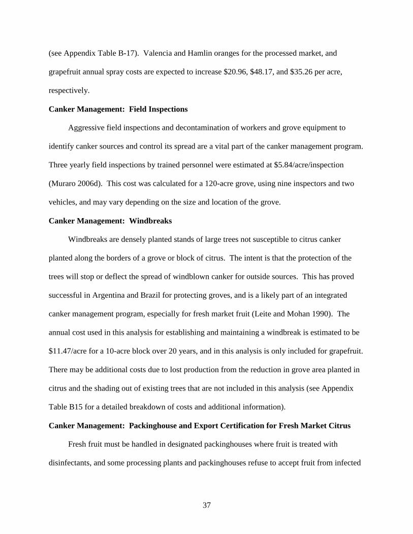
Figure 3-1. Indonesian citrus production, 1975-2005
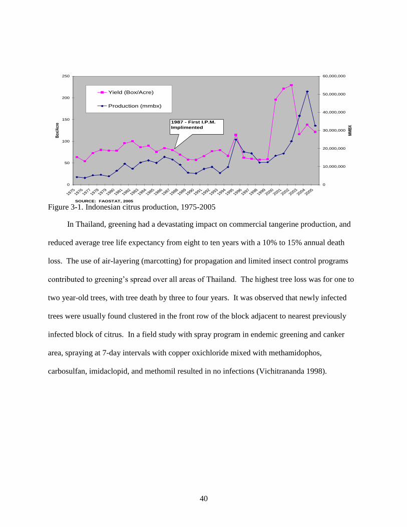
In Thailand, greening had a devastating impact on commercial tangerine production, and
reduced average tree life expectancy from eight to ten years with a 10% to 15% annual death
loss. The use of air-layering (marcotting) for propagation and limited insect control programs
contributed to greening’s spread over all areas of Thailand. The highest tree loss was for one to
two year-old trees, with tree death by three to four years. It was observed that newly infected
trees were usually found clustered in the front row of the block adjacent to nearest previously
infected block of citrus. In a field study with spray program in endemic greening and canker
area, spraying at 7-day intervals with copper oxichloride mixed with methamidophos,
carbosulfan, imidaclopid, and methomil resulted in no infections (Vichitrananda 1998).
41
Figure 3-2. Thai citrus production, 1975-2005
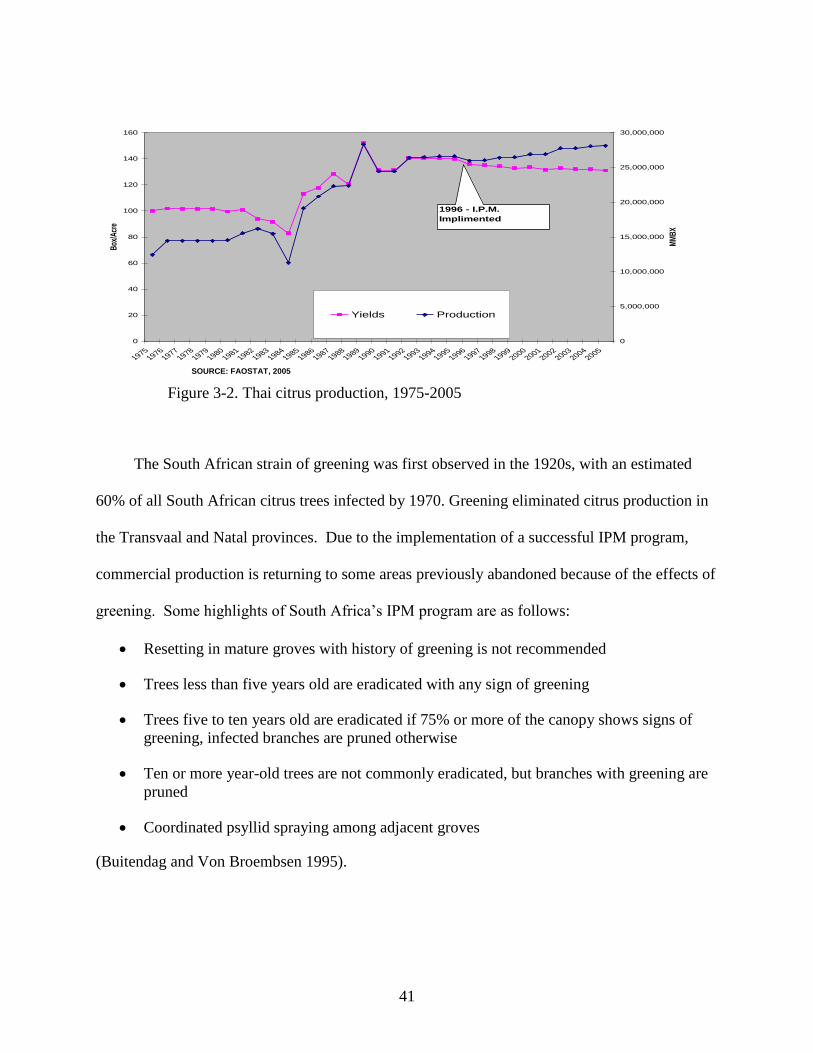
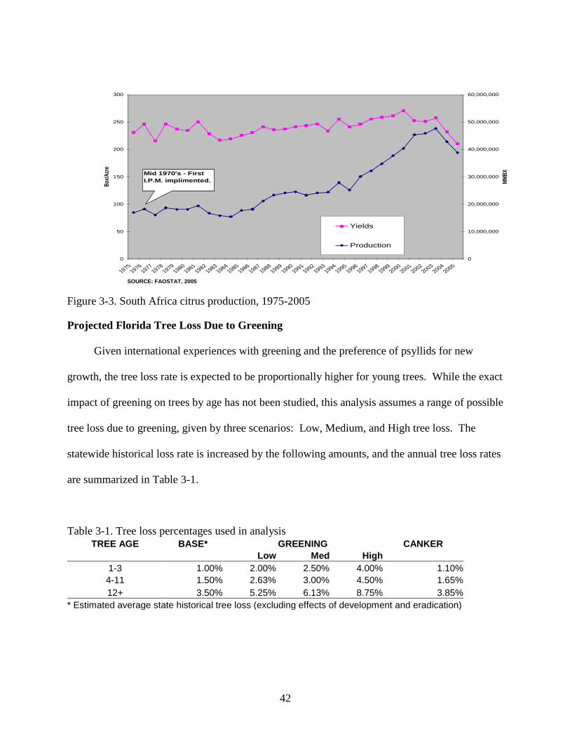
The South African strain of greening was first observed in the 1920s, with an estimated
60% of all South African citrus trees infected by 1970. Greening eliminated citrus production in
the Transvaal and Natal provinces. Due to the implementation of a successful IPM program,
commercial production is returning to some areas previously abandoned because of the effects of
greening. Some highlights of South Africa’s IPM program are as follows:
Resetting in mature groves with history of greening is not recommended
Trees less than five years old are eradicated with any sign of greening
Trees five to ten years old are eradicated if 75% or more of the canopy shows signs of
greening, infected branches are pruned otherwise
Ten or more year-old trees are not commonly eradicated, but branches with greening are
pruned
Coordinated psyllid spraying among adjacent groves
(Buitendag and Von Broembsen 1995).
THAILAND CITRUS 1975-2005
0
20
40
60
80
100
120
140
160
19751976
19771978
19791980
19811982
19831984
19851986
19871988
19891990
19911992
19931994
19951996
19971998
19992000
20012002
20032004
2005
Box
/Acr
e
0
5,000,000
10,000,000
15,000,000
20,000,000
25,000,000
30,000,000
MM
BX
Yields Production
1996 - I.P.M.
Implimented
SOURCE: FAOSTAT, 2005
42
Figure 3-3. South Africa citrus production, 1975-2005
Projected Florida Tree Loss Due to Greening
Given international experiences with greening and the preference of psyllids for new
growth, the tree loss rate is expected to be proportionally higher for young trees. While the exact
impact of greening on trees by age has not been studied, this analysis assumes a range of possible
tree loss due to greening, given by three scenarios: Low, Medium, and High tree loss. The
statewide historical loss rate is increased by the following amounts, and the annual tree loss rates
are summarized in Table 3-1.
Table 3-1. Tree loss percentages used in analysis TREE AGE BASE* GREENING CANKER
Low Med High
1-3 1.00% 2.00% 2.50% 4.00% 1.10%
4-11 1.50% 2.63% 3.00% 4.50% 1.65%
12+ 3.50% 5.25% 6.13% 8.75% 3.85%
* Estimated average state historical tree loss (excluding effects of development and eradication)
SOUTH AFRICA CITRUS 1975-2005
0
50
100
150
200
250
300
19751976
19771978
19791980
19811982
19831984
19851986
19871988
19891990
19911992
19931994
19951996
19971998
19992000
20012002
20032004
2005
Box
/Acr
e
0
10,000,000
20,000,000
30,000,000
40,000,000
50,000,000
60,000,000
MM
BX
Yields
Production
Mid 1970's - First
I.P.M. implimented.
SOURCE: FAOSTAT, 2005
43
Greening Management: Psyllid Control
The psyllid insect vector of greening is difficult to control because the psyllid population
spikes at certain times of the year, exhibits continuous movement between citrus trees and
surrounding host vegetation, and has a wide range of other host plants besides citrus. Moreover,
its small size and recent arrival to Florida makes it difficult for growers not familiar with the
insect to discover its presence in the grove. Psyllids feed almost exclusively on new growth
flushes, and adult psyllids are able to acquire and transmit greening within 24 to 48 hours
(Buitendag and Broembsen 1992). The importance of a coordinated psyllid IPM was illustrated
in Indian field tests that found that 67% of certified greening-free trees were infected three years
after planting if greening was present on adjoining properties (Azzaro et al. 1993). Chinese
researchers successfully eliminated all greening incidents by the eradication of all backyard
citrus and other host plants in area, the use of windbreaks, the planting of certified greening-free
trees, the application of ten to thirteen psyllid-specific sprays per year in flush periods, and the
prohibited introduction of any host plants in general area (Ke and Xu 1990). Another Chinese
study tested the possibility of rehabilitation of an infected grove by pruning all infected branches
and applying 10 to 13 psyllid specific sprays per year. This resulted in reducing new infections
from 2.5% to 1% over eleven years in one location, and 7% to 1% over nine years in the other
(Xu et al. 1991). Moreover, ten to twenty psyllid-specific sprays per year does not appear to be
feasible for both economic and environmental reasons.
From the international experience with greening, a South African study of different psyllid
control programs found that:
Multiple sprays aimed at maintaining low populations of psylla throughout the spring,
summer, and autumn periods were impractical and caused pest repercussions. It was then
realized that systemic treatments targeted specifically at psylla and applied either to the
stem or to the roots would be most effective (Buitendag and Von Broembsen 1992).
44
Experiments in psyllid control in Florida have shown that foliar applied insecticides such as
Danitol, Lorsban, and petroleum oils are useful for short-term control of spikes in psyllid
populations, while foliar or soil-applied systemic insecticides such as Provado, Temik, and
Admire are useful for long-term control. Admire is used on young, non-bearing trees, and Temik
is used on older, productive trees (Rodgers 2006). To augment the standard citrus spray
program, this analysis assumes annual Temik or Admire applications in their maximum
allowable amounts, plus one additional Danitol and Lorsban application per year. This results in
a cost increase of $203.00/acre for oranges on the Ridge, $194.36/acre for oranges on the
Flatwoods, and $156.74/acre for grapefruit, added to the existing grove spray program results in
the chemical costs shown in Appendix Table B17. The grapefruit for fresh market costs do not
increase as much as the oranges for processing because of the ability to combine greening spray
applications with the existing spray program.
Greening Management: Grove Inspections
Greening’s ease of transmission makes it necessary to scout aggressively for signs of
psyllids and infected trees. Infected trees should be eradicated immediately, and psyllid
populations controlled promptly to avoid a quick spread throughout the grove (Brlansky 2005).
This analysis assumes that growers must inspect six times per year. Using the same cost
components as the canker inspection program described above, the annual cost of greening
inspections is $35.04/acre.
Combining the Effects of Canker and Greening
To account for the combined effects of canker and greening in a grove, the above cost
categories, yield, and tree loss assumptions are added together and overlaps, particularly in the
spray programs are subtracted. A comparison of spray programs with different disease scenarios
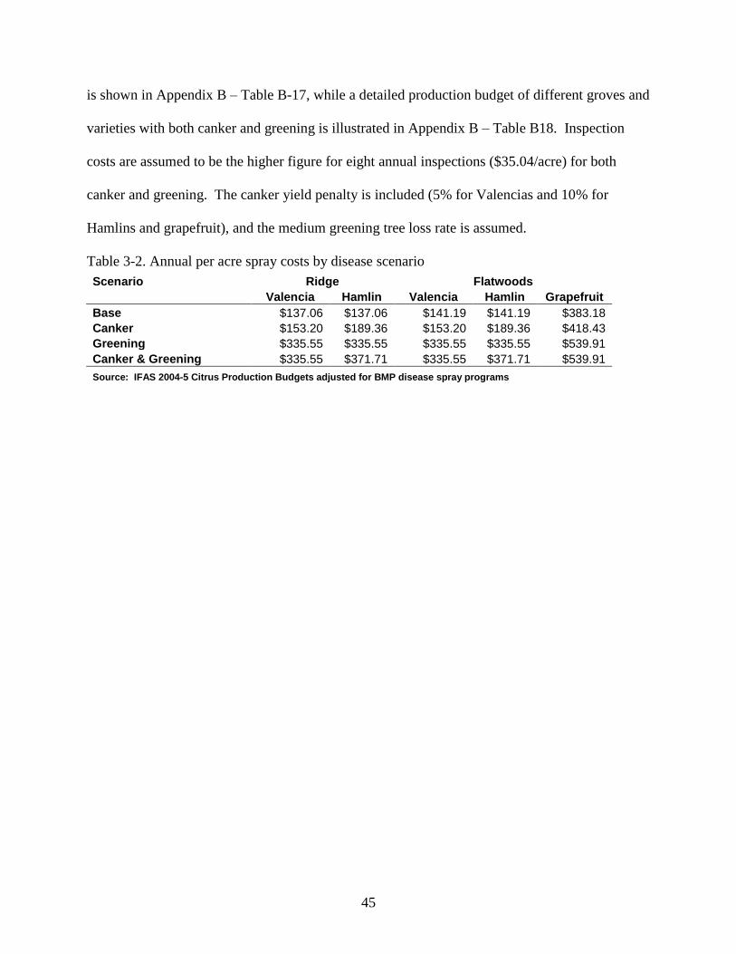
45
is shown in Appendix B – Table B-17, while a detailed production budget of different groves and
varieties with both canker and greening is illustrated in Appendix B – Table B18. Inspection
costs are assumed to be the higher figure for eight annual inspections ($35.04/acre) for both
canker and greening. The canker yield penalty is included (5% for Valencias and 10% for
Hamlins and grapefruit), and the medium greening tree loss rate is assumed.
Table 3-2. Annual per acre spray costs by disease scenario
Scenario Ridge Flatwoods
Valencia Hamlin Valencia Hamlin Grapefruit
Base $137.06 $137.06 $141.19 $141.19 $383.18
Canker $153.20 $189.36 $153.20 $189.36 $418.43
Greening $335.55 $335.55 $335.55 $335.55 $539.91
Canker & Greening $335.55 $371.71 $335.55 $371.71 $539.91
Source: IFAS 2004-5 Citrus Production Budgets adjusted for BMP disease spray programs
46
CHAPTER 4
A NET PRESENT VALUE MODEL OF A FLORIDA CITRUS GROVE
The definition of an investment used in this analysis is the ownership of an asset that has
value. The value of an asset is created by intrinsic value and/or the value of the income it may
produce. Unless this asset is inherited or received as a gift, the ownership of the asset must be
purchased with another asset of value. In this analysis, value is framed in monetary (dollar)
terms. The preferred goal of an investment is to capture a return that is in excess of what it costs
to obtain the asset.
In the case of an investment in a citrus grove, initial costs are incurred in the purchase of
the land and establishment of the trees. This is based upon the expectation of creating value
from the future income from the production of the fruit and the ownership of a productive grove.
Due to the long life of a productive grove, it is necessary to determine the value of the future
production and ownership currently to compare it to the costs that are incurred now. Net present
value analysis is a means of comparing the future expected returns to ownership of a citrus grove
to the current cost of acquiring it.
A citrus grove is a dynamic enterprise where yields, revenues, costs, and grove value
change through time depending on tree age, tree loss, fruit prices, and input costs. This analysis
adapts a mixed-age grove model to reflect grove operating costs and revenues. This mixed-age
grove model captures the evolution of costs over time, including the costs of tree loss, resetting,
and caring for replacement trees. Both box and pound solids yields increase with tree age, and
with resetting it is necessary to capture the effect of a mix of tree ages on total grove yields.
Accounting for trees of different ages within a grove becomes even more important when higher
tree loss assumptions due to disease are incorporated. Generalized examples of the model’s
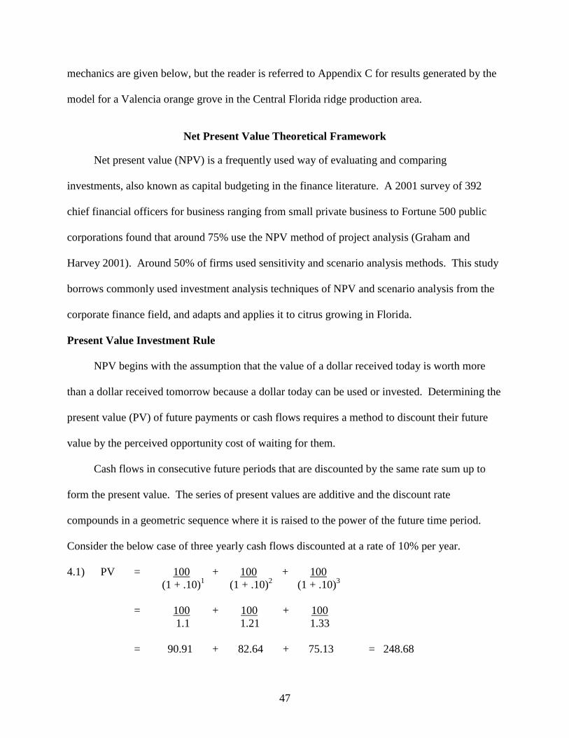
47
mechanics are given below, but the reader is referred to Appendix C for results generated by the
model for a Valencia orange grove in the Central Florida ridge production area.
Net Present Value Theoretical Framework
Net present value (NPV) is a frequently used way of evaluating and comparing
investments, also known as capital budgeting in the finance literature. A 2001 survey of 392
chief financial officers for business ranging from small private business to Fortune 500 public
corporations found that around 75% use the NPV method of project analysis (Graham and
Harvey 2001). Around 50% of firms used sensitivity and scenario analysis methods. This study
borrows commonly used investment analysis techniques of NPV and scenario analysis from the
corporate finance field, and adapts and applies it to citrus growing in Florida.
Present Value Investment Rule
NPV begins with the assumption that the value of a dollar received today is worth more
than a dollar received tomorrow because a dollar today can be used or invested. Determining the
present value (PV) of future payments or cash flows requires a method to discount their future
value by the perceived opportunity cost of waiting for them.
Cash flows in consecutive future periods that are discounted by the same rate sum up to
form the present value. The series of present values are additive and the discount rate
compounds in a geometric sequence where it is raised to the power of the future time period.
Consider the below case of three yearly cash flows discounted at a rate of 10% per year.
4.1) PV = 100 + 100 + 100
(1 + .10)1 (1 + .10)
2 (1 + .10)
3
= 100 + 100 + 100
1.1 1.21 1.33
= 90.91 + 82.64 + 75.13 = 248.68
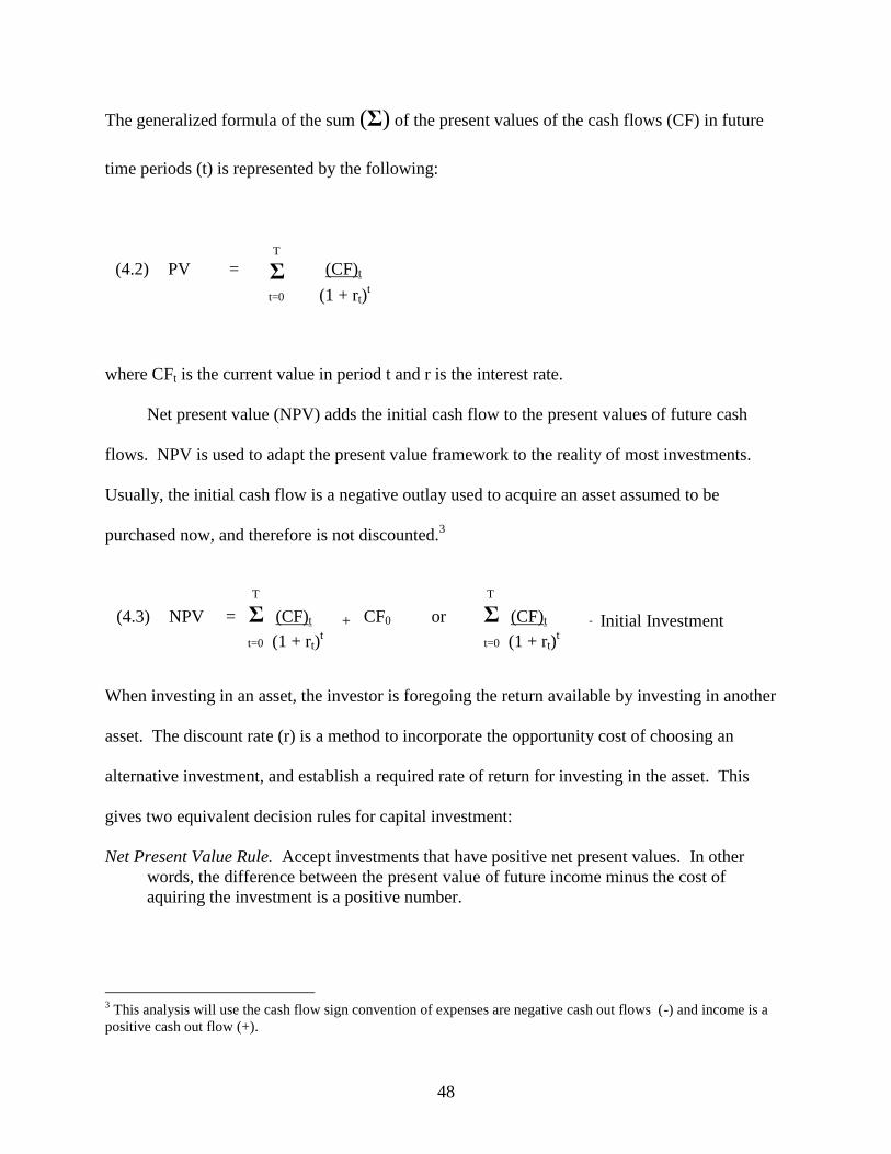
48
The generalized formula of the sum (Σ) of the present values of the cash flows (CF) in future
time periods (t) is represented by the following:
where CFt is the current value in period t and r is the interest rate.
Net present value (NPV) adds the initial cash flow to the present values of future cash
flows. NPV is used to adapt the present value framework to the reality of most investments.
Usually, the initial cash flow is a negative outlay used to acquire an asset assumed to be
purchased now, and therefore is not discounted.3
When investing in an asset, the investor is foregoing the return available by investing in another
asset. The discount rate (r) is a method to incorporate the opportunity cost of choosing an
alternative investment, and establish a required rate of return for investing in the asset. This
gives two equivalent decision rules for capital investment:
Net Present Value Rule. Accept investments that have positive net present values. In other
words, the difference between the present value of future income minus the cost of
aquiring the investment is a positive number.
3 This analysis will use the cash flow sign convention of expenses are negative cash out flows (-) and income is a
positive cash out flow (+).
T
(4.2) PV = Σ (CF)t
t=0 (1 + rt)t
T T
(4.3) NPV = Σ (CF)t + CF0 or Σ (CF)t - Initial Investment
t=0 (1 + rt)t t=0 (1 + rt)
t
49
Rate-of-Return Rule. Accept investments that offer rates of return in excess of their opportunity
costs of capital, or the rate of return of the investment exceeds the rates of return on similar
investments.
Alternative Investment Rules
Three traditional alternatives to the NPV investment decision rule are the book rate of
return, payback period, and internal rate of return (or hurdle rate) (Brealey and Meyers 2003).
These rules are commonly used and may lead to misleading conclusions and incorrect decisions
based on their results. It is important to remember that NPV depends only on forecasted cash
flows and the discount rate or opportunity cost of capital.
Book income is another name for accounting income, and it used to determine the book
rate of return. Book income is commonly shown on a firm or individual’s income statement, and
book assets and shareholder’s equity are shown on the balance sheet. Both are reported using
accrual accounting methods which may not reflect actual cash inflows and outflows. The book
rate of return is the basis for ratios such as the return on assets (ROA) or return on equity (ROE).
Accounting procedures separate cash outflows into capital and operating expenses. Capital
expenditures are depreciated and debited against income according to a schedule that may not
reflect the actual cash flows; also, the allocation of capital and operating expenditures is usually
reported across an entire firm or individual’s income and balance sheet, and not on an individual
project or investment basis. When evaluating a capital investment decision, it is important to
remove the distortive effects of the choice of accounting methods from the actual value of the
investment; however, there are benefits to tax, depreciation, and financing choices. Elsewhere,
this analysis includes a framework for how to calculate these ancillary benefits.
(4.4) Book rate of return = Book Income or Book Income
Book Assets Shareholder’s Equity
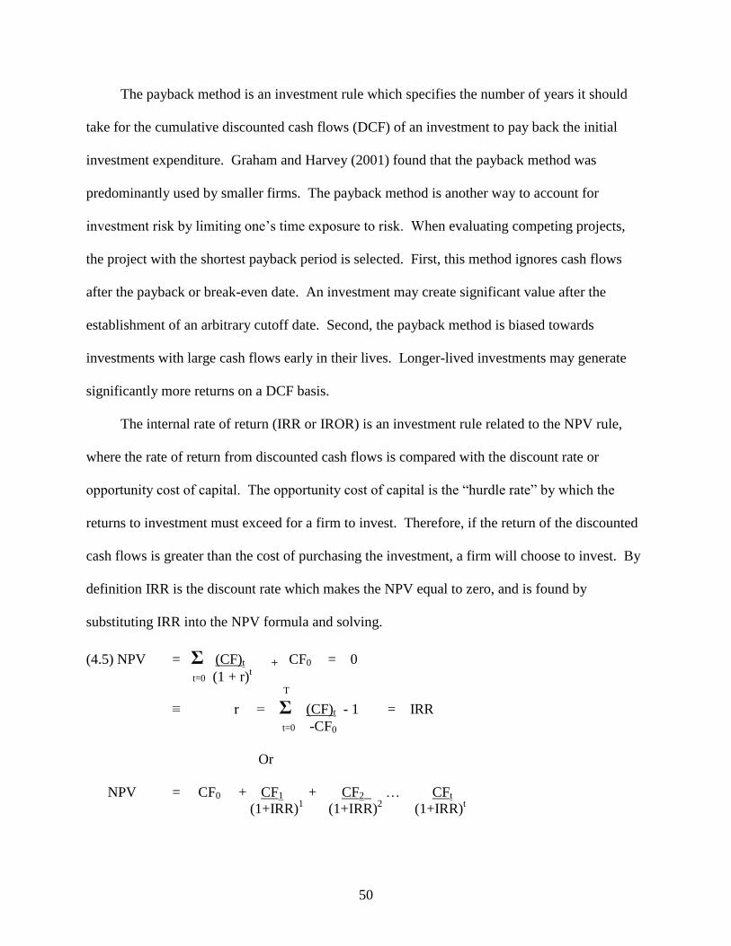
50
The payback method is an investment rule which specifies the number of years it should
take for the cumulative discounted cash flows (DCF) of an investment to pay back the initial
investment expenditure. Graham and Harvey (2001) found that the payback method was
predominantly used by smaller firms. The payback method is another way to account for
investment risk by limiting one’s time exposure to risk. When evaluating competing projects,
the project with the shortest payback period is selected. First, this method ignores cash flows
after the payback or break-even date. An investment may create significant value after the
establishment of an arbitrary cutoff date. Second, the payback method is biased towards
investments with large cash flows early in their lives. Longer-lived investments may generate
significantly more returns on a DCF basis.
The internal rate of return (IRR or IROR) is an investment rule related to the NPV rule,
where the rate of return from discounted cash flows is compared with the discount rate or
opportunity cost of capital. The opportunity cost of capital is the “hurdle rate” by which the
returns to investment must exceed for a firm to invest. Therefore, if the return of the discounted
cash flows is greater than the cost of purchasing the investment, a firm will choose to invest. By
definition IRR is the discount rate which makes the NPV equal to zero, and is found by
substituting IRR into the NPV formula and solving.
(4.5) NPV = Σ (CF)t + CF0 = 0
t=0 (1 + r)t
T
≡ r = Σ (CF)t - 1 = IRR
t=0 -CF0
Or
NPV = CF0 + CF1 + CF2 … CFt
(1+IRR)1 (1+IRR)
2 (1+IRR)
t
51
The IRR illustrates the important aspect of NPV which is its inverse relationship to the
discount rate. As the discount rate increases, the present value of future cash flows decreases
and NPV becomes smaller. This relationship can be represented by the downward sloping line
shown in Figure 4.1. Where the line crosses the discount rate axis is where the NPV of an
investment is equal to zero. That rate is the IRR, in this case 35%. The IRR must be compared
to the discount rate to either accept or reject the investment. For example, if the discount rate (r)
is 20%, the opportunity cost of capital is less than the internal rate of return to the investment
(IRR) of 35%, and the NPV is +$1,200. Therefore, the investment will be accepted. If the
discount rate (r) is 65%, the opportunity cost of capital is greater than the IRR (35%), and the
NPV is -$1,000. Therefore, the investment will be rejected.
Figure 4-1. Relationship of NPV and IRR
The IRR is a polynomial equation for multiple periods, has no unique solution, and must
be solved numerically through interpolation to find an accurate value. Fortunately, this can be
done instantly through the use of spreadsheet-based computer programs or financial calculators.
Unfortunately, an investment’s NPV function is not always as smooth as the line in Figure 4.1.
The IRR method will give an inaccurate figure if there are changes of signs in the cash flow, or
+2,000
+1,000
-1,000
-2,000
Discount
Rate (%)
Net Present Value ($)
25% 100%
25
%
75%
25%
25
%
50%
25%
25
%
IRR = 35%
Firm’s NPV r = 20%
NPV=+1,200
r = 65%
NPV=-1,000
0
52
large positive cash flows early in the investment’s life. For instance, if there are many swings
where the DCF’s go from positive to negative, this may give multiple IRR’s if the function
crosses the discount rate axis more than one time. The IRR is calculated in citrus grove
investment analysis because it can be useful in some situations to compare the profitability of an
investment to its opportunity cost, but NPV is a more reliable measure of value over time and an
absolute measure of the total value created.
Adapting NPV to Citrus Investment
To adapt the NPV framework to a citrus investment, it is first necessary to construct the
cash flows. In its most basic form, the cash flow to growing citrus is a function of yield, price,
and cost. In each period there exists a yield of fruit which is multiplied by the price for the fruit
minus the operating cost. The first period (period 0) is typically referred to as the initial
investment. This is the cash out flow necessary to acquire the grove whether it is the purchase of
a mature grove or the cost for establishing a new or replanted grove. In this analysis, it is
necessary to distinguish two indexing variables of time (t) and tree age (a). Time is the analysis
time which starts in year 0 (present day) and moves forward 15 years or periods. This is distinct
from tree age (a) which will change depending on the beginning age distribution of the grove and
amount of tree loss incorporated into the model. Yields and costs change with time, tree age,
variety (V), tree loss (Ψ), and the presence of disease (θ). In this case, the disease considered is
either canker or greening, and is separated from normal tree loss in a grove. Price (P) is treated
as an exogenous variable and is used to measure the effects of changes is yield and cost due to
disease.
53
Exiting the Investment: Bond Valuation, Perpetuities, and Terminal Value
The additive property of present value makes it an attractive method for determining the
value of an asset with a long series of future cash flows. Although, one must determine a cash
flow for each period of the asset’s expected life. This becomes difficult and time consuming
when the asset has a very long or indefinite life. A well-maintained citrus grove is usually
expected to last at least fifteen years to thirty years, and may last much longer. A grove owner
expects that the grove will retain a terminal value as an income producing property after the
expected life of the grove due to its suitability to be replanted in citrus. This creates an issue of
how to determine the present value of all the future returns accruing to ownership of a grove.
The method of valuing of one of the most basic financial instruments, the bond, illustrates
a path to valuing a citrus investment. A fixed-coupon bond is a debt instrument similar to loan
where the holder of the bond is entitled to a fixed series of interest payments (coupons) until the
bond matures at a specific date and the holder receives the face value (principal) of the bond.
The bond can be viewed as two investments, and discounted separately.
The value of the bond (or a citrus investment) depends on the coupon payments (income),
the principal (value of investment), the time to maturity (expected life of the grove), and the
(4.8) PV(bond) = PV(coupon payments) + PV(principal)
(4.6) -CF0 = Initial Investment
(4.7) CFt = P Yt - Ct, where Y(t, a, V, Ψ , θ) and C (t, a, V, Ψ, θ)
t = analysis time period
a = tree age
V = tree variety
Ψ = tree loss
θ = disease effect
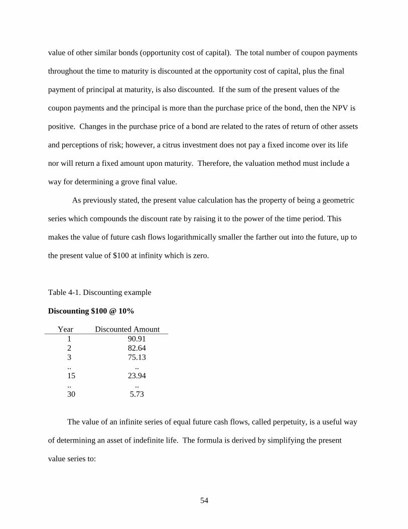
54
value of other similar bonds (opportunity cost of capital). The total number of coupon payments
throughout the time to maturity is discounted at the opportunity cost of capital, plus the final
payment of principal at maturity, is also discounted. If the sum of the present values of the
coupon payments and the principal is more than the purchase price of the bond, then the NPV is
positive. Changes in the purchase price of a bond are related to the rates of return of other assets
and perceptions of risk; however, a citrus investment does not pay a fixed income over its life
nor will return a fixed amount upon maturity. Therefore, the valuation method must include a
way for determining a grove final value.
As previously stated, the present value calculation has the property of being a geometric
series which compounds the discount rate by raising it to the power of the time period. This
makes the value of future cash flows logarithmically smaller the farther out into the future, up to
the present value of $100 at infinity which is zero.
Table 4-1. Discounting example
Discounting $100 @ 10%
Year Discounted Amount
1 90.91
2 82.64
3 75.13
.. ..
15 23.94
.. ..
30 5.73
The value of an infinite series of equal future cash flows, called perpetuity, is a useful way
of determining an asset of indefinite life. The formula is derived by simplifying the present
value series to:
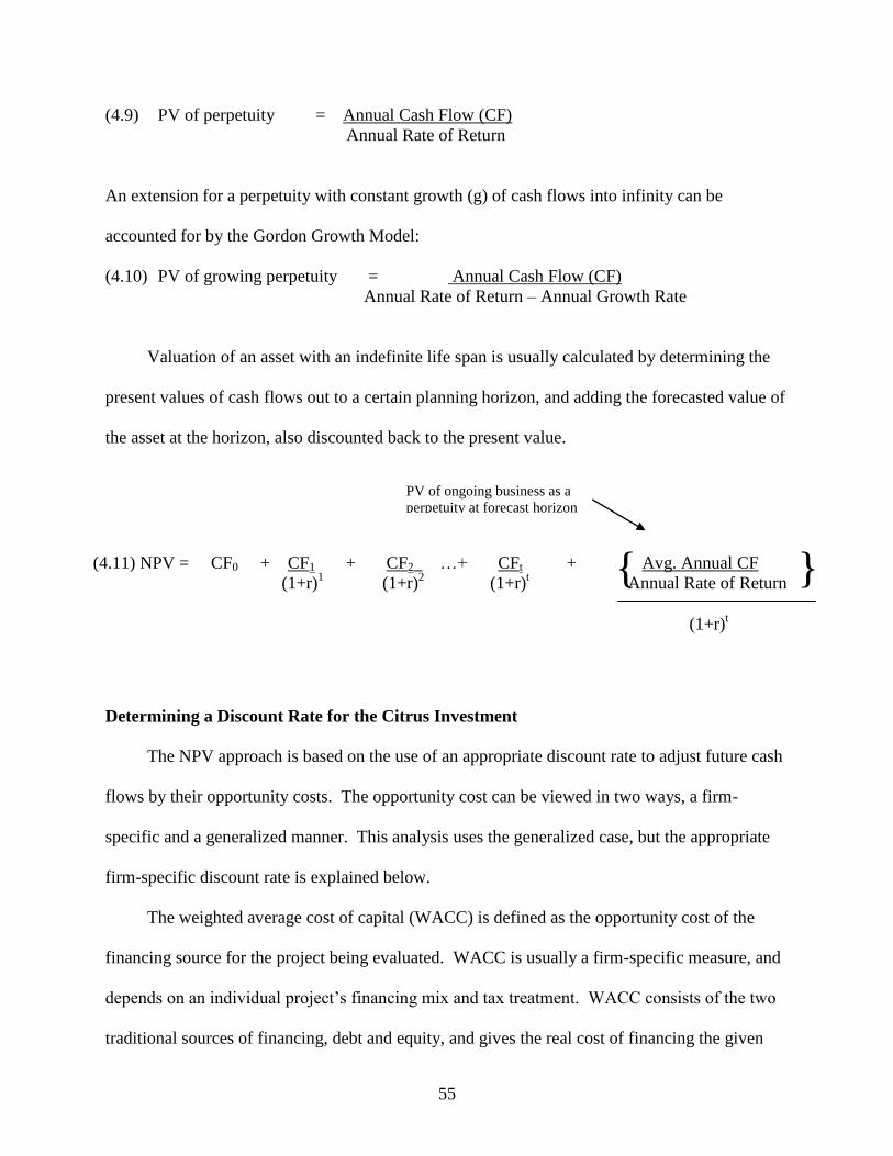
55
(4.9) PV of perpetuity = Annual Cash Flow (CF)
Annual Rate of Return
An extension for a perpetuity with constant growth (g) of cash flows into infinity can be
accounted for by the Gordon Growth Model:
(4.10) PV of growing perpetuity = Annual Cash Flow (CF)
Annual Rate of Return – Annual Growth Rate
Valuation of an asset with an indefinite life span is usually calculated by determining the
present values of cash flows out to a certain planning horizon, and adding the forecasted value of
the asset at the horizon, also discounted back to the present value.
Determining a Discount Rate for the Citrus Investment
The NPV approach is based on the use of an appropriate discount rate to adjust future cash
flows by their opportunity costs. The opportunity cost can be viewed in two ways, a firm-
specific and a generalized manner. This analysis uses the generalized case, but the appropriate
firm-specific discount rate is explained below.
The weighted average cost of capital (WACC) is defined as the opportunity cost of the
financing source for the project being evaluated. WACC is usually a firm-specific measure, and
depends on an individual project’s financing mix and tax treatment. WACC consists of the two
traditional sources of financing, debt and equity, and gives the real cost of financing the given
{ }
(4.11) NPV = CF0 + CF1 + CF2 …+ CFt + Avg. Annual CF
(1+r)1 (1+r)
2 (1+r)
t Annual Rate of Return
(1+r)t
PV of ongoing business as a
perpetuity at forecast horizon
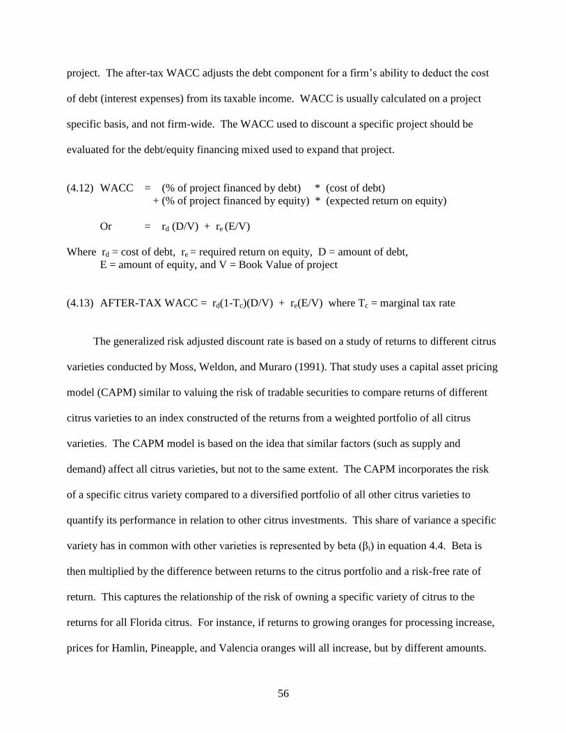
56
project. The after-tax WACC adjusts the debt component for a firm’s ability to deduct the cost
of debt (interest expenses) from its taxable income. WACC is usually calculated on a project
specific basis, and not firm-wide. The WACC used to discount a specific project should be
evaluated for the debt/equity financing mixed used to expand that project.
(4.12) WACC = (% of project financed by debt) * (cost of debt)
+ (% of project financed by equity) * (expected return on equity)
Or = rd (D/V) + re (E/V)
Where rd = cost of debt, re = required return on equity, D = amount of debt,
E = amount of equity, and V = Book Value of project
(4.13) AFTER-TAX WACC = rd(1-Tc)(D/V) + re(E/V) where Tc = marginal tax rate
The generalized risk adjusted discount rate is based on a study of returns to different citrus
varieties conducted by Moss, Weldon, and Muraro (1991). That study uses a capital asset pricing
model (CAPM) similar to valuing the risk of tradable securities to compare returns of different
citrus varieties to an index constructed of the returns from a weighted portfolio of all citrus
varieties. The CAPM model is based on the idea that similar factors (such as supply and
demand) affect all citrus varieties, but not to the same extent. The CAPM incorporates the risk
of a specific citrus variety compared to a diversified portfolio of all other citrus varieties to
quantify its performance in relation to other citrus investments. This share of variance a specific
variety has in common with other varieties is represented by beta (βi) in equation 4.4. Beta is
then multiplied by the difference between returns to the citrus portfolio and a risk-free rate of
return. This captures the relationship of the risk of owning a specific variety of citrus to the
returns for all Florida citrus. For instance, if returns to growing oranges for processing increase,
prices for Hamlin, Pineapple, and Valencia oranges will all increase, but by different amounts.
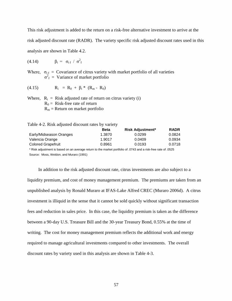
57
This risk adjustment is added to the return on a risk-free alternative investment to arrive at the
risk adjusted discount rate (RADR). The variety specific risk adjusted discount rates used in this
analysis are shown in Table 4.2.
(4.14) βi = σi f / σ2
f
Where, σi f = Covariance of citrus variety with market portfolio of all varieties
σ2
f = Variance of market portfolio
(4.15) Ri = R0 + βi * (Rm - R0)
Where, Ri = Risk adjusted rate of return on citrus variety (i)
R0 = Risk-free rate of return
Rm = Return on market portfolio
Table 4-2. Risk adjusted discount rates by variety Beta Risk Adjustment* RADR
Early/Midseason Oranges 1.3870 0.0299 0.0824
Valencia Orange 1.9017 0.0409 0.0934
Colored Grapefruit 0.8961 0.0193 0.0718
* Risk adjustment is based on an average return to the market portfolio of .0743 and a risk-free rate of .0525
Source: Moss, Weldon, and Muraro (1991)
In addition to the risk adjusted discount rate, citrus investments are also subject to a
liquidity premium, and cost of money management premium. The premiums are taken from an
unpublished analysis by Ronald Muraro at IFAS-Lake Alfred CREC (Muraro 2006d). A citrus
investment is illiquid in the sense that it cannot be sold quickly without significant transaction
fees and reduction in sales price. In this case, the liquidity premium is taken as the difference
between a 90-day U.S. Treasure Bill and the 30-year Treasury Bond, 0.55% at the time of
writing. The cost for money management premium reflects the additional work and energy
required to manage agricultural investments compared to other investments. The overall
discount rates by variety used in this analysis are shown in Table 4-3.
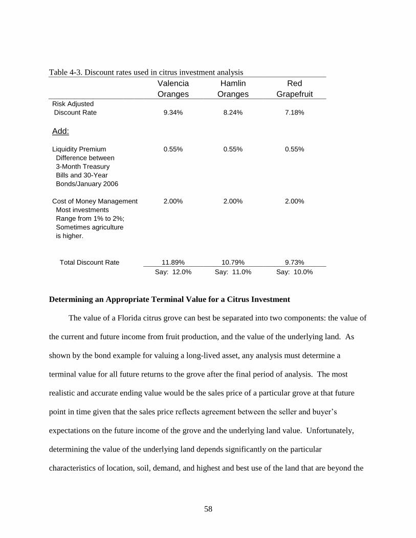
58
Table 4-3. Discount rates used in citrus investment analysis
Valencia Hamlin Red
Oranges Oranges Grapefruit Risk Adjusted
Discount Rate 9.34% 8.24% 7.18%
Add:
Liquidity Premium 0.55% 0.55% 0.55%
Difference between
3-Month Treasury
Bills and 30-Year
Bonds/January 2006
Cost of Money Management 2.00% 2.00% 2.00%
Most investments
Range from 1% to 2%;
Sometimes agriculture
is higher.
Total Discount Rate 11.89% 10.79% 9.73%
Say: 12.0% Say: 11.0% Say: 10.0%
Determining an Appropriate Terminal Value for a Citrus Investment
The value of a Florida citrus grove can best be separated into two components: the value of
the current and future income from fruit production, and the value of the underlying land. As
shown by the bond example for valuing a long-lived asset, any analysis must determine a
terminal value for all future returns to the grove after the final period of analysis. The most
realistic and accurate ending value would be the sales price of a particular grove at that future
point in time given that the sales price reflects agreement between the seller and buyer’s
expectations on the future income of the grove and the underlying land value. Unfortunately,
determining the value of the underlying land depends significantly on the particular
characteristics of location, soil, demand, and highest and best use of the land that are beyond the
59
scope of this analysis; however, information exists about grove income and we can arrive at a
reasonable approximation of a terminal value to include in this analysis.
The valuation (or appraisal) of land and real estate property is commonly divided into three
analysis approaches that are subsequently compared to determine a fair market value for the
property (The Appraisal Institute 2001). First, the extraction or cost approach values the
replacement or reproduction cost of structures and improvements to land given that the utility of
the structures or improvements can be exactly reproduced. For agricultural properties, the cost
approach is usually not applicable because of the low percentage of the total value of the
property that is attributable to structures and improvements (Muraro 1989). Second, the income
approach values a property by its income producing potential and converts the value of all future
income accruing to ownership of the property to a present value through the capitalization rate.
This is the main approach this analysis will use. Third, the market or comparable sales approach
estimates the value of the property by observing the values of like properties, and adjusting for
particular aspects of the sale, such as location, transaction date, land characteristics, and the
terms of sale. While the comparable sales approach is only applicable to specific properties, this
analysis will use that approach to validate an applicable capitalization rate.
The income approach to citrus valuation starts by deriving an average annual expected
income from the property, net of grove and operating expenses. This is divided by the sale price
of the land to determine a capitalization (or cap) rate. The cap rate can be thought of as the
annual return on investment, and is positively related to increases in net income and negatively
related to increases in the sales price. Note, the cap rate only includes income, and not changes
in the selling price of the land over time (capital gain or loss). Since this analysis is generalized
to a variety of grove circumstances, the actual sale price of the grove is unknown, but is assumed
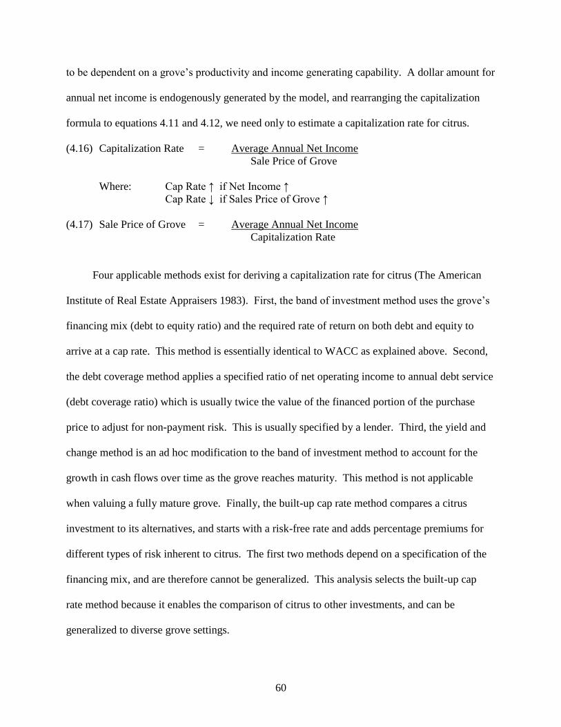
60
to be dependent on a grove’s productivity and income generating capability. A dollar amount for
annual net income is endogenously generated by the model, and rearranging the capitalization
formula to equations 4.11 and 4.12, we need only to estimate a capitalization rate for citrus.
(4.16) Capitalization Rate = Average Annual Net Income
Sale Price of Grove
Where: Cap Rate ↑ if Net Income ↑
Cap Rate ↓ if Sales Price of Grove ↑
(4.17) Sale Price of Grove = Average Annual Net Income
Capitalization Rate
Four applicable methods exist for deriving a capitalization rate for citrus (The American
Institute of Real Estate Appraisers 1983). First, the band of investment method uses the grove’s
financing mix (debt to equity ratio) and the required rate of return on both debt and equity to
arrive at a cap rate. This method is essentially identical to WACC as explained above. Second,
the debt coverage method applies a specified ratio of net operating income to annual debt service
(debt coverage ratio) which is usually twice the value of the financed portion of the purchase
price to adjust for non-payment risk. This is usually specified by a lender. Third, the yield and
change method is an ad hoc modification to the band of investment method to account for the
growth in cash flows over time as the grove reaches maturity. This method is not applicable
when valuing a fully mature grove. Finally, the built-up cap rate method compares a citrus
investment to its alternatives, and starts with a risk-free rate and adds percentage premiums for
different types of risk inherent to citrus. The first two methods depend on a specification of the
financing mix, and are therefore cannot be generalized. This analysis selects the built-up cap
rate method because it enables the comparison of citrus to other investments, and can be
generalized to diverse grove settings.
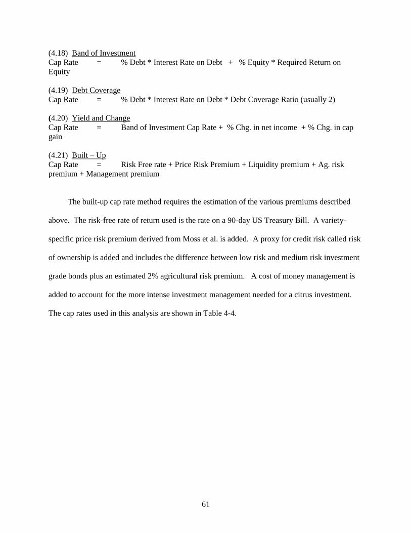
61
(4.18) Band of Investment
Cap Rate = % Debt * Interest Rate on Debt + % Equity * Required Return on
Equity
(4.19) Debt Coverage
Cap Rate = % Debt * Interest Rate on Debt * Debt Coverage Ratio (usually 2)
(4.20) Yield and Change
Cap Rate = Band of Investment Cap Rate + % Chg. in net income + % Chg. in cap
gain
(4.21) Built – Up
Cap Rate = Risk Free rate + Price Risk Premium + Liquidity premium + Ag. risk
premium + Management premium
The built-up cap rate method requires the estimation of the various premiums described
above. The risk-free rate of return used is the rate on a 90-day US Treasury Bill. A variety-
specific price risk premium derived from Moss et al. is added. A proxy for credit risk called risk
of ownership is added and includes the difference between low risk and medium risk investment
grade bonds plus an estimated 2% agricultural risk premium. A cost of money management is
added to account for the more intense investment management needed for a citrus investment.
The cap rates used in this analysis are shown in Table 4-4.
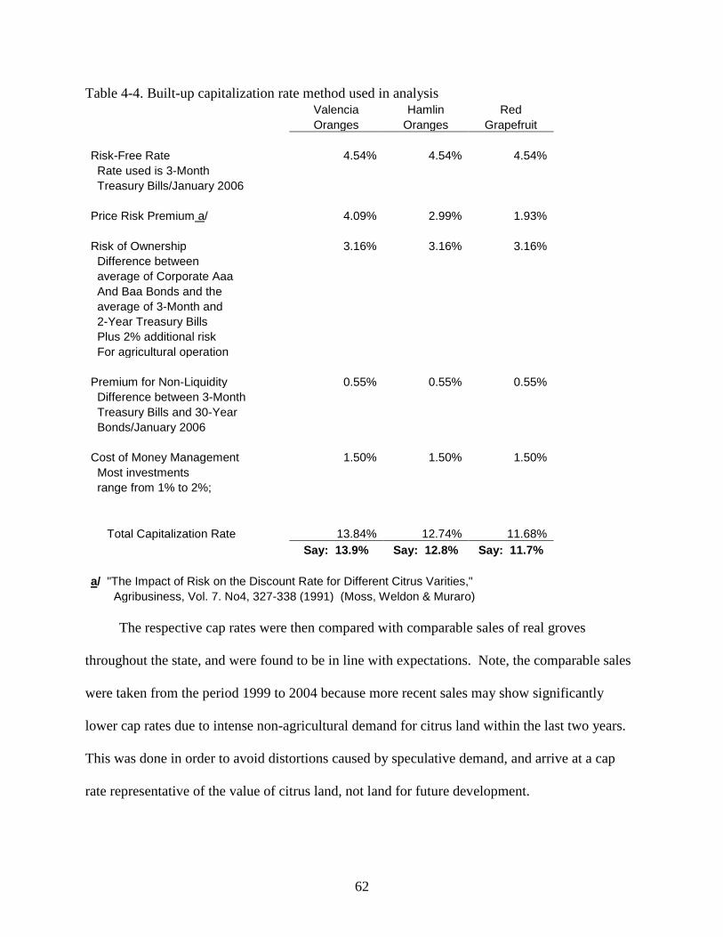
62
Table 4-4. Built-up capitalization rate method used in analysis Valencia Hamlin Red
Oranges Oranges Grapefruit
Risk-Free Rate 4.54% 4.54% 4.54%
Rate used is 3-Month
Treasury Bills/January 2006
Price Risk Premium a/ 4.09% 2.99% 1.93%
Risk of Ownership 3.16% 3.16% 3.16%
Difference between
average of Corporate Aaa
And Baa Bonds and the
average of 3-Month and
2-Year Treasury Bills
Plus 2% additional risk
For agricultural operation
Premium for Non-Liquidity 0.55% 0.55% 0.55%
Difference between 3-Month
Treasury Bills and 30-Year
Bonds/January 2006
Cost of Money Management 1.50% 1.50% 1.50%
Most investments
range from 1% to 2%;
Total Capitalization Rate 13.84% 12.74% 11.68%
Say: 13.9% Say: 12.8% Say: 11.7%
a/ "The Impact of Risk on the Discount Rate for Different Citrus Varities,"
Agribusiness, Vol. 7. No4, 327-338 (1991) (Moss, Weldon & Muraro)
The respective cap rates were then compared with comparable sales of real groves
throughout the state, and were found to be in line with expectations. Note, the comparable sales
were taken from the period 1999 to 2004 because more recent sales may show significantly
lower cap rates due to intense non-agricultural demand for citrus land within the last two years.
This was done in order to avoid distortions caused by speculative demand, and arrive at a cap
rate representative of the value of citrus land, not land for future development.
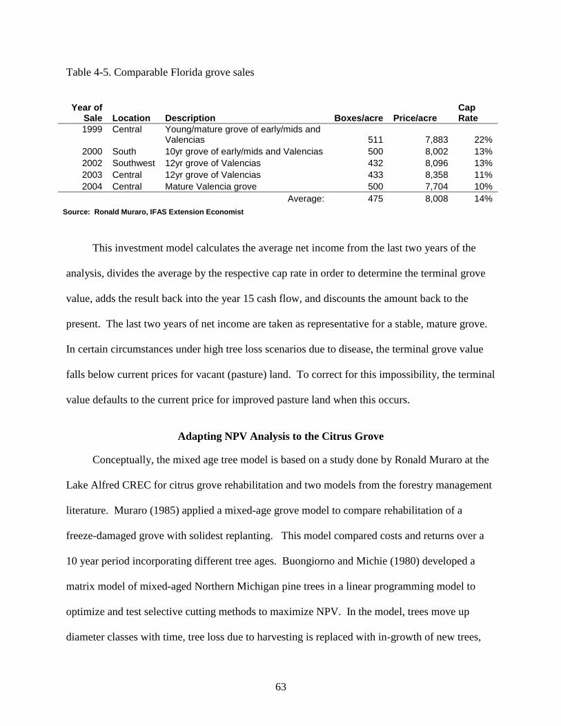
63
Table 4-5. Comparable Florida grove sales
This investment model calculates the average net income from the last two years of the
analysis, divides the average by the respective cap rate in order to determine the terminal grove
value, adds the result back into the year 15 cash flow, and discounts the amount back to the
present. The last two years of net income are taken as representative for a stable, mature grove.
In certain circumstances under high tree loss scenarios due to disease, the terminal grove value
falls below current prices for vacant (pasture) land. To correct for this impossibility, the terminal
value defaults to the current price for improved pasture land when this occurs.
Adapting NPV Analysis to the Citrus Grove
Conceptually, the mixed age tree model is based on a study done by Ronald Muraro at the
Lake Alfred CREC for citrus grove rehabilitation and two models from the forestry management
literature. Muraro (1985) applied a mixed-age grove model to compare rehabilitation of a
freeze-damaged grove with solidest replanting. This model compared costs and returns over a
10 year period incorporating different tree ages. Buongiorno and Michie (1980) developed a
matrix model of mixed-aged Northern Michigan pine trees in a linear programming model to
optimize and test selective cutting methods to maximize NPV. In the model, trees move up
diameter classes with time, tree loss due to harvesting is replaced with in-growth of new trees,
Year of Sale Location Description Boxes/acre Price/acre
Cap Rate
1999 Central Young/mature grove of early/mids and Valencias 511 7,883 22%
2000 South 10yr grove of early/mids and Valencias 500 8,002 13%
2002 Southwest 12yr grove of Valencias 432 8,096 13%
2003 Central 12yr grove of Valencias 433 8,358 11%
2004 Central Mature Valencia grove 500 7,704 10%
Average: 475 8,008 14%
Source: Ronald Muraro, IFAS Extension Economist
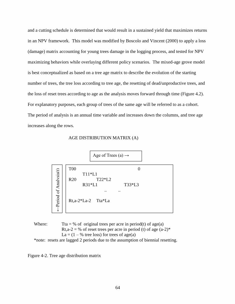
64
and a cutting schedule is determined that would result in a sustained yield that maximizes returns
in an NPV framework. This model was modified by Boscolo and Vincent (2000) to apply a loss
(damage) matrix accounting for young trees damage in the logging process, and tested for NPV
maximizing behaviors while overlaying different policy scenarios. The mixed-age grove model
is best conceptualized as based on a tree age matrix to describe the evolution of the starting
number of trees, the tree loss according to tree age, the resetting of dead/unproductive trees, and
the loss of reset trees according to age as the analysis moves forward through time (Figure 4.2).
For explanatory purposes, each group of trees of the same age will be referred to as a cohort.
The period of analysis is an annual time variable and increases down the columns, and tree age
increases along the rows.
Figure 4-2. Tree age distribution matrix
T00 0
T11*L1
R20 T22*L2
R31*L1 T33*L3
.. ..
Rt,a-2*La-2 Tta*La
Age of Trees (a) →
←P
erio
d o
f A
nal
ysi
s(t)
Where: Tta = % of original trees per acre in period(t) of age(a)
Rt,a-2 = % of reset trees per acre in period (t) of age (a-2)*
La = (1 – % tree loss) for trees of age(a)
*note: resets are lagged 2 periods due to the assumption of biennial resetting.
AGE DISTRIBUTION MATRIX (A)
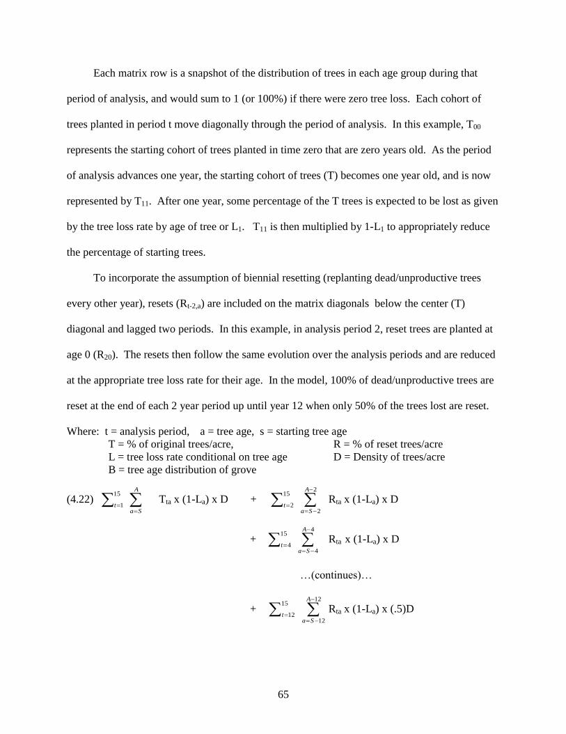
65
Each matrix row is a snapshot of the distribution of trees in each age group during that
period of analysis, and would sum to 1 (or 100%) if there were zero tree loss. Each cohort of
trees planted in period t move diagonally through the period of analysis. In this example, T00
represents the starting cohort of trees planted in time zero that are zero years old. As the period
of analysis advances one year, the starting cohort of trees (T) becomes one year old, and is now
represented by T11. After one year, some percentage of the T trees is expected to be lost as given
by the tree loss rate by age of tree or L1. T11 is then multiplied by 1-L1 to appropriately reduce
the percentage of starting trees.
To incorporate the assumption of biennial resetting (replanting dead/unproductive trees
every other year), resets (Rt-2,a) are included on the matrix diagonals below the center (T)
diagonal and lagged two periods. In this example, in analysis period 2, reset trees are planted at
age 0 (R20). The resets then follow the same evolution over the analysis periods and are reduced
at the appropriate tree loss rate for their age. In the model, 100% of dead/unproductive trees are
reset at the end of each 2 year period up until year 12 when only 50% of the trees lost are reset.
Where: t = analysis period, a = tree age, s = starting tree age
T = % of original trees/acre, R = % of reset trees/acre
L = tree loss rate conditional on tree age D = Density of trees/acre
B = tree age distribution of grove
(4.22)
A
Sat
15
1 Tta x (1-La) x D +
2
2
15
2
A
Sat
Rta x (1-La) x D
+
4
4
15
4
A
Sat
Rta x (1-La) x D
…(continues)…
+
12
12
15
12
A
Sat
Rta x (1-La) x (.5)D
66
+
14
14
15
14
A
Sat
Rta x (1-La) x (.5)D
=
15
0t
Bt
This is due to the opinion that higher density plantings will be maturing at around 10 years
of age, and the older original trees will shade out the young reset trees if spaced too closely
together (Muraro 2006 IV).
Calculating Yields for a Mixed-Age Grove
The per-acre yields given by a mixed age grove can be considered an extension of the age
distribution equation above. As trees age, box production per tree increases, also, pound solids
per box increase with tree age. In equation (2), an additional term for box yield per tree and
pound solid per box by tree age is added to each tree age cohort. This captures the differences in
yields between trees planted at different times. Appendix B - Table B2 illustrates the yield
distribution by tree age for Valencia oranges on the Ridge.
(4.23)
A
at
0
15
0 Tta x (1-La) x D x Ya x Sa +
2
2
15
2
A
sat
Rta x (1-La) x D x Ya x Sa
…(continues same as previous equation)…
= Total boxes per acret
= Total pounds-solid per acret
Where Ya is boxes per tree for a tree of age a and Sa is pound-solids per box for a tree of age a.
Determining Grove Production Costs
This analysis works with the assumption of the use of precision agriculture in grove
management, and applies the tree age matrix to adjusting costs by tree age. First, mature grove
costs for a 10+ year old grove are determined for the base and disease scenarios based on IFAS
67
citrus production budgets. Cost categories that vary by tree age are cultivation and herbicide,
spraying/chemicals, fertilization, pruning/topping/hedging, and irrigation. The costs are adjusted
by tree age according to the schedule in Appendix B, Table B8 – Grove Cost Adjustment by Tree
Age.
Solidset grove costs for years 1 through 4 of tree age are determined separately for the base
and disease scenarios. If the grove is being solidset, the model charges planting costs for special
cultivation and herbicide applications(years 1-4), tree wrap maintenance (years 1-3), labor for
cutting sprouts (years 1-2), Ridomil/Aliete application for foot rot (years 1-2), tree cost, and one
time charges for staking, planting, tree wrap, and first watering of the tree. Spray/chemical costs
are adjusted according to the above schedule (see Appendix B, Table B3 - Solidset Costs by
Disease Scenario).
Reset costs for year 1 through 3 are determined separately for the base and disease
scenarios. As stated in Chapter 1, reset trees incur supplemental costs in addition to normal
grove care costs for about the first three years of life. Supplemental reset costs include
maintenance and cultivation (for years 1-3), and one-time planting charges for site preparation,
dead/unproductive tree removal, nursery tree cost, staking, planting, and first watering the tree.
These costs are in addition to the normal costs incurred for 1 to 3 year old trees.
To incorporate changes in the grove care costs due to tree loss and resetting, a matrix
approach is used to provide a simple and dynamic method for adjusting total costs by the number
of trees of each age. A grove care budget is created for the grove adjusted by tree age from
planting to 15 years of age (see Appendix B, Table B5 - New Planting/Replanting Operating
Cost Budget for Valencia Grove).
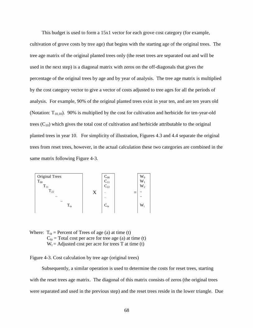
68
This budget is used to form a 15x1 vector for each grove cost category (for example,
cultivation of grove costs by tree age) that begins with the starting age of the original trees. The
tree age matrix of the original planted trees only (the reset trees are separated out and will be
used in the next step) is a diagonal matrix with zeros on the off-diagonals that gives the
percentage of the original trees by age and by year of analysis. The tree age matrix is multiplied
by the cost category vector to give a vector of costs adjusted to tree ages for all the periods of
analysis. For example, 90% of the original planted trees exist in year ten, and are ten years old
(Notation: T10,10). 90% is multiplied by the cost for cultivation and herbicide for ten-year-old
trees (C10) which gives the total cost of cultivation and herbicide attributable to the original
planted trees in year 10. For simplicity of illustration, Figures 4.3 and 4.4 separate the original
trees from reset trees, however, in the actual calculation these two categories are combined in the
same matrix following Figure 4-3.
Figure 4-3. Cost calculation by tree age (original trees)
Subsequently, a similar operation is used to determine the costs for reset trees, starting
with the reset trees age matrix. The diagonal of this matrix consists of zeros (the original trees
were separated and used in the previous step) and the reset trees reside in the lower triangle. Due
X =
Where: Tta = Percent of Trees of age (a) at time (t)
Cta = Total cost per acre for tree age (a) at time (t)
Wt = Adjusted cost per acre for trees T at time (t)
Original Trees
T00
T11
T22
..
..
Tta
C00
C11
C22
..
..
Cta
W0
W1
W2
..
..
Wt
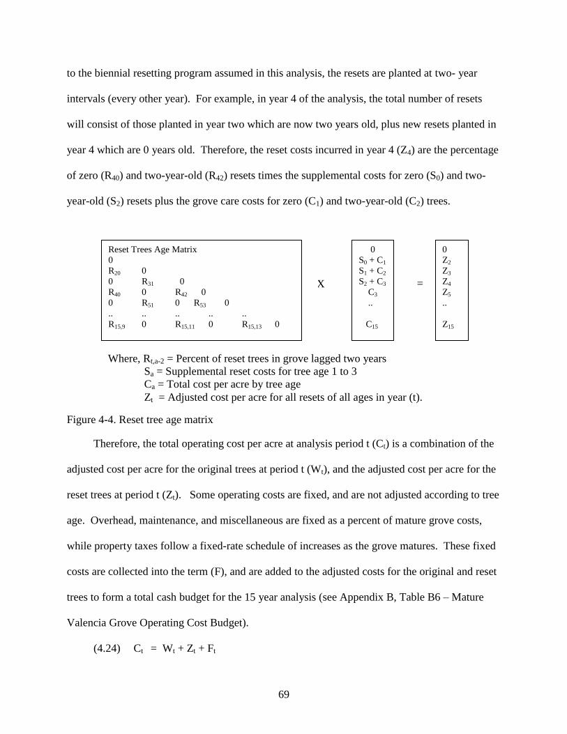
69
to the biennial resetting program assumed in this analysis, the resets are planted at two- year
intervals (every other year). For example, in year 4 of the analysis, the total number of resets
will consist of those planted in year two which are now two years old, plus new resets planted in
year 4 which are 0 years old. Therefore, the reset costs incurred in year 4 (Z4) are the percentage
of zero (R40) and two-year-old (R42) resets times the supplemental costs for zero (S0) and two-
year-old (S2) resets plus the grove care costs for zero (C1) and two-year-old (C2) trees.
Figure 4-4. Reset tree age matrix
Therefore, the total operating cost per acre at analysis period t (Ct) is a combination of the
adjusted cost per acre for the original trees at period t (Wt), and the adjusted cost per acre for the
reset trees at period t (Zt). Some operating costs are fixed, and are not adjusted according to tree
age. Overhead, maintenance, and miscellaneous are fixed as a percent of mature grove costs,
while property taxes follow a fixed-rate schedule of increases as the grove matures. These fixed
costs are collected into the term (F), and are added to the adjusted costs for the original and reset
trees to form a total cash budget for the 15 year analysis (see Appendix B, Table B6 – Mature
Valencia Grove Operating Cost Budget).
(4.24) Ct = Wt + Zt + Ft
Reset Trees Age Matrix
0
R20 0
0 R31 0
R40 0 R42 0
0 R51 0 R53 0
.. .. .. .. ..
R15,9 0 R15,11 0 R15,13 0
0
S0 + C1
S1 + C2
S2 + C3
C3
..
C15
0
Z2
Z3
Z4
Z5
..
Z15
X =
Where, Rt,a-2 = Percent of reset trees in grove lagged two years
Sa = Supplemental reset costs for tree age 1 to 3
Ca = Total cost per acre by tree age
Zt = Adjusted cost per acre for all resets of all ages in year (t).
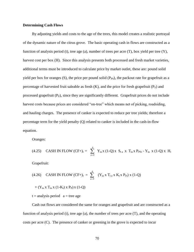
70
Determining Cash Flows
By adjusting yields and costs to the age of the trees, this model creates a realistic portrayal
of the dynamic nature of the citrus grove. The basic operating cash in flows are constructed as a
function of analysis period (t), tree age (a), number of trees per acre (T), box yield per tree (Y),
harvest cost per box (H). Since this analysis presents both processed and fresh market varieties,
additional terms must be introduced to calculate price by market outlet, these are: pound solid
yield per box for oranges (S), the price per pound solid (PPS), the packout rate for grapefruit as a
percentage of harvested fruit saleable as fresh (K), and the price for fresh grapefruit (PF) and
processed grapefruit (PP), since they are significantly different. Grapefruit prices do not include
harvest costs because prices are considered “on-tree” which means net of picking, roadsiding,
and hauling charges. The presence of canker is expected to reduce per tree yields; therefore a
percentage term for the yield penalty (Q) related to canker is included in the cash-in-flow
equation.
Oranges:
(4.25) CASH IN FLOW (CF+)t =
A
a 0
Yta x (1-Q) x St a x Tta x PPSt - Yta x (1-Q) x Ht
Grapefruit:
(4.26) CASH IN FLOW (CF+)t =
A
a 0
(Yta x Tt a x Kt x PFt) x (1-Q)
+ (Yta x Tta x (1-Kt) x PP) x (1-Q)
t = analysis period a = tree age
Cash out flows are considered the same for oranges and grapefruit and are constructed as a
function of analysis period (t), tree age (a), the number of trees per acre (T), and the operating
costs per acre (C). The presence of canker or greening in the grove is expected to incur
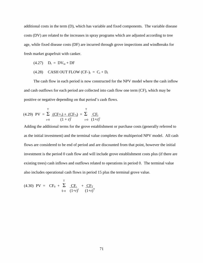
71
additional costs in the term (D), which has variable and fixed components. The variable disease
costs (DV) are related to the increases in spray programs which are adjusted according to tree
age, while fixed disease costs (DF) are incurred through grove inspections and windbreaks for
fresh market grapefruit with canker.
(4.27) Dt = DVta + DF
(4.28) CASH OUT FLOW (CF-)t = Ct + Dt
The cash flow in each period is now constructed for the NPV model where the cash inflow
and cash outflows for each period are collected into cash flow one term (CF), which may be
positive or negative depending on that period’s cash flows.
Adding the additional terms for the grove establishment or purchase costs (generally referred to
as the initial investment) and the terminal value completes the multiperiod NPV model. All cash
flows are considered to be end of period and are discounted from that point, however the initial
investment is the period 0 cash flow and will include grove establishment costs plus (if there are
existing trees) cash inflows and outflows related to operations in period 0. The terminal value
also includes operational cash flows in period 15 plus the terminal grove value.
T
(4.30) PV = CF0 + Σ CFt + CFT
t=0 (1+r)t
(1+r)T
T T
(4.29) PV = Σ (CF+t) + (CF-t) = Σ CFt
t=0 (1 + r)t
t=0 (1+r)t
72
CHAPTER 5
EMPIRICAL RESULTS
Alternative scenarios are constructed to develop hypothetical situations currently faced
by Florida growers. First, investment scenarios are determined based on either new plantings
(with and without land costs), or mature plantings without land costs. Then, the production costs
and yields detailed in Chapter 2 are established for Hamlin and Valencia sweet oranges grown
for the processing (juice) market on both ridge and flatwoods locations, and colored (Red or
Pink) grapefruit grown for the fresh fruit market on an Indian River location. Finally,
assumptions are applied for additional costs, yield decline, and tree losses due to the different
diseases. In Appendix B, detailed cost budgets illustrate the Solidset Costs (Table B-3) of grove
care expenses for the first four years of a new Valencia planting. Appendix B tables B-15, B-16,
and B-17 show annual mature grove production costs with the canker, greening, and canker and
greening diseases scenarios, respectively. Actual production costs are reported in Appendix B
(Tables B-5 and B-6) for a Valencia ridge grove, and vary from the annual figures because of
adjustments for tree age, tree loss, and resetting.
The return on investment is determined at different price levels for citrus using a net
present value framework over a 15 year period of analysis. Price is assumed to remain constant
over the analysis period. In this respect, price serves as an indicator of the effects of changing
costs and disease scenarios. The breakeven prices reported are the lowest prices where the NPV
of the grove is positive over the 15 year period. All calculations are performed on a per-acre
basis.
Results of the Mixed-Age Grove Model – Yield and Cost Analysis
For a new planting of citrus, initial planting (solidset) costs are included in grove expenses.
These costs include initial tree and planting costs, as well as the previously indicated young tree
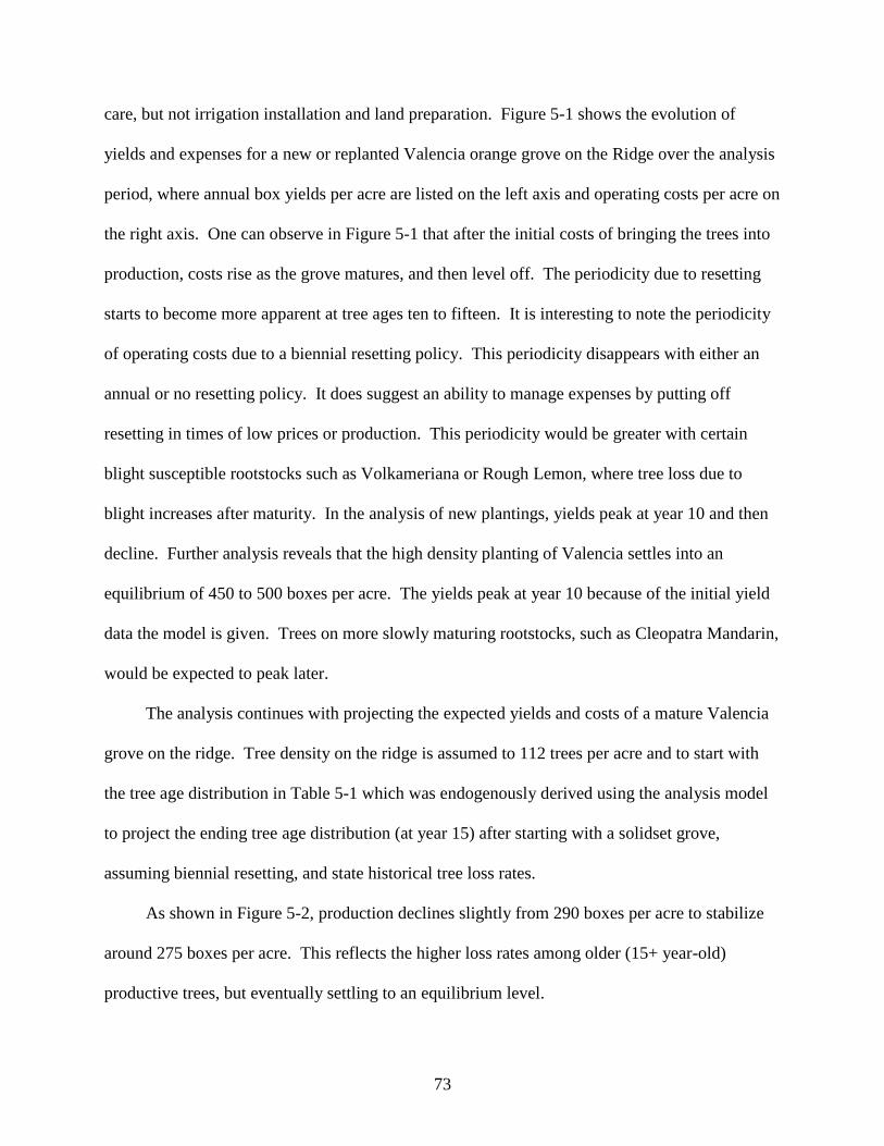
73
care, but not irrigation installation and land preparation. Figure 5-1 shows the evolution of
yields and expenses for a new or replanted Valencia orange grove on the Ridge over the analysis
period, where annual box yields per acre are listed on the left axis and operating costs per acre on
the right axis. One can observe in Figure 5-1 that after the initial costs of bringing the trees into
production, costs rise as the grove matures, and then level off. The periodicity due to resetting
starts to become more apparent at tree ages ten to fifteen. It is interesting to note the periodicity
of operating costs due to a biennial resetting policy. This periodicity disappears with either an
annual or no resetting policy. It does suggest an ability to manage expenses by putting off
resetting in times of low prices or production. This periodicity would be greater with certain
blight susceptible rootstocks such as Volkameriana or Rough Lemon, where tree loss due to
blight increases after maturity. In the analysis of new plantings, yields peak at year 10 and then
decline. Further analysis reveals that the high density planting of Valencia settles into an
equilibrium of 450 to 500 boxes per acre. The yields peak at year 10 because of the initial yield
data the model is given. Trees on more slowly maturing rootstocks, such as Cleopatra Mandarin,
would be expected to peak later.
The analysis continues with projecting the expected yields and costs of a mature Valencia
grove on the ridge. Tree density on the ridge is assumed to 112 trees per acre and to start with
the tree age distribution in Table 5-1 which was endogenously derived using the analysis model
to project the ending tree age distribution (at year 15) after starting with a solidset grove,
assuming biennial resetting, and state historical tree loss rates.
As shown in Figure 5-2, production declines slightly from 290 boxes per acre to stabilize
around 275 boxes per acre. This reflects the higher loss rates among older (15+ year-old)
productive trees, but eventually settling to an equilibrium level.
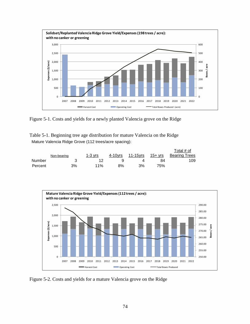
74
Figure 5-1. Costs and yields for a newly planted Valencia grove on the Ridge
Table 5-1. Beginning tree age distribution for mature Valencia on the Ridge
Mature Valencia Ridge Grove (112 trees/acre spacing):
Total # of Bearing Trees Non-bearing 1-3 yrs 4-10yrs 11-15yrs 15+ yrs
Number 3 12 9 4 84 109
Percent 3% 11% 8% 3% 75%
Figure 5-2. Costs and yields for a mature Valencia grove on the Ridge
0
100
200
300
400
500
600
0
500
1,000
1,500
2,000
2,500
3,000
2007 2008 2009 2010 2011 2012 2013 2014 2015 2016 2017 2018 2019 2020 2021 2022
Bo
xes
/ ac
re
Exp
en
ses
($/a
cre
)
Harvest Cost Operating Cost Total Boxes Produced (acre)
Solidset/Replanted Valencia Ridge Grove Yield/Expenses (198 trees / acre):with no canker or greening
250.00
255.00
260.00
265.00
270.00
275.00
280.00
285.00
290.00
0
500
1,000
1,500
2,000
2,500
2007 2008 2009 2010 2011 2012 2013 2014 2015 2016 2017 2018 2019 2020 2021 2022
Bo
xes
/ ac
re
Exp
en
ses
($/a
cre
)
Harvest Cost Operating Cost Total Boxes Produced
Mature Valencia Ridge Grove Yield/Expenses (112 trees / acre):with no canker or greening
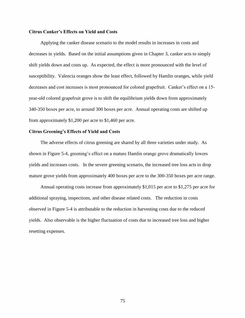
75
Citrus Canker’s Effects on Yield and Costs
Applying the canker disease scenario to the model results in increases in costs and
decreases in yields. Based on the initial assumptions given in Chapter 3, canker acts to simply
shift yields down and costs up. As expected, the effect is more pronounced with the level of
susceptibility. Valencia oranges show the least effect, followed by Hamlin oranges, while yield
decreases and cost increases is most pronounced for colored grapefruit. Canker’s effect on a 15-
year-old colored grapefruit grove is to shift the equilibrium yields down from approximately
340-350 boxes per acre, to around 300 boxes per acre. Annual operating costs are shifted up
from approximately $1,200 per acre to $1,460 per acre.
Citrus Greening’s Effects of Yield and Costs
The adverse effects of citrus greening are shared by all three varieties under study. As
shown in Figure 5-4, greening’s effect on a mature Hamlin orange grove dramatically lowers
yields and increases costs. In the severe greening scenario, the increased tree loss acts to drop
mature grove yields from approximately 400 boxes per acre to the 300-350 boxes per acre range.
Annual operating costs increase from approximately $1,015 per acre to $1,275 per acre for
additional spraying, inspections, and other disease related costs. The reduction in costs
observed in Figure 5-4 is attributable to the reduction in harvesting costs due to the reduced
yields. Also observable is the higher fluctuation of costs due to increased tree loss and higher
resetting expenses.
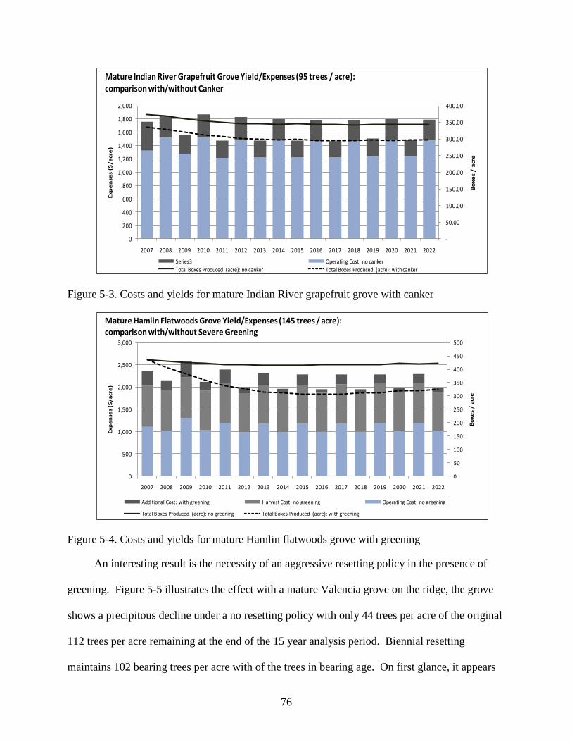
76
Figure 5-3. Costs and yields for mature Indian River grapefruit grove with canker
Figure 5-4. Costs and yields for mature Hamlin flatwoods grove with greening
An interesting result is the necessity of an aggressive resetting policy in the presence of
greening. Figure 5-5 illustrates the effect with a mature Valencia grove on the ridge, the grove
shows a precipitous decline under a no resetting policy with only 44 trees per acre of the original
112 trees per acre remaining at the end of the 15 year analysis period. Biennial resetting
maintains 102 bearing trees per acre with of the trees in bearing age. On first glance, it appears
-
50.00
100.00
150.00
200.00
250.00
300.00
350.00
400.00
0
200
400
600
800
1,000
1,200
1,400
1,600
1,800
2,000
2007 2008 2009 2010 2011 2012 2013 2014 2015 2016 2017 2018 2019 2020 2021 2022
Bo
xe
s /
acr
e
Ex
pe
nse
s ($
/a
cre
)
Series3 Operating Cost: no canker
Total Boxes Produced (acre): no canker Total Boxes Produced (acre): with canker
Mature Indian River Grapefruit Grove Yield/Expenses (95 trees / acre):comparison with/without Canker
0
50
100
150
200
250
300
350
400
450
500
0
500
1,000
1,500
2,000
2,500
3,000
2007 2008 2009 2010 2011 2012 2013 2014 2015 2016 2017 2018 2019 2020 2021 2022
Bo
xe
s /
acr
e
Exp
en
ses
($/a
cre
)
Additional Cost: with greening Harvest Cost: no greening Operating Cost: no greening
Total Boxes Produced (acre): no greening Total Boxes Produced (acre): with greening
Mature Hamlin Flatwoods Grove Yield/Expenses (145 trees / acre):comparison with/without Severe Greening
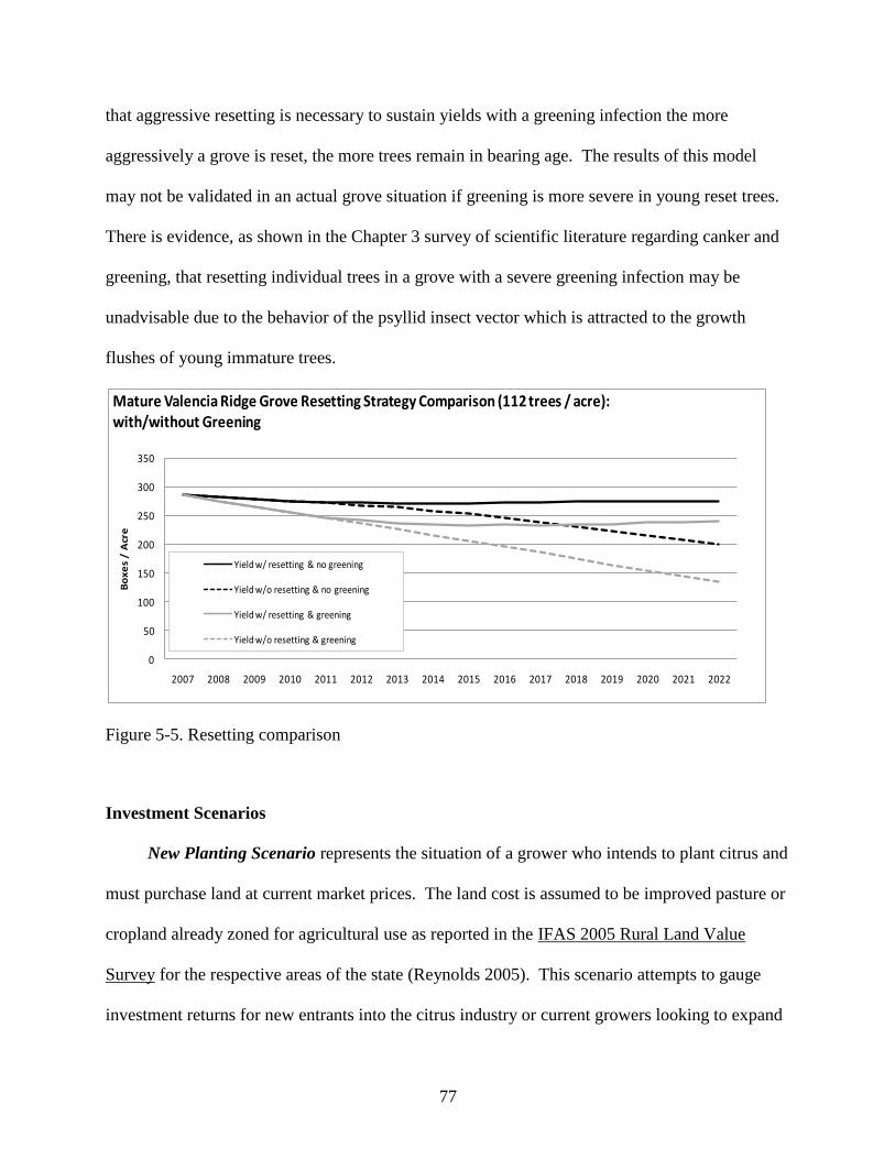
77
that aggressive resetting is necessary to sustain yields with a greening infection the more
aggressively a grove is reset, the more trees remain in bearing age. The results of this model
may not be validated in an actual grove situation if greening is more severe in young reset trees.
There is evidence, as shown in the Chapter 3 survey of scientific literature regarding canker and
greening, that resetting individual trees in a grove with a severe greening infection may be
unadvisable due to the behavior of the psyllid insect vector which is attracted to the growth
flushes of young immature trees.
Figure 5-5. Resetting comparison
Investment Scenarios
New Planting Scenario represents the situation of a grower who intends to plant citrus and
must purchase land at current market prices. The land cost is assumed to be improved pasture or
cropland already zoned for agricultural use as reported in the IFAS 2005 Rural Land Value
Survey for the respective areas of the state (Reynolds 2005). This scenario attempts to gauge
investment returns for new entrants into the citrus industry or current growers looking to expand
0
50
100
150
200
250
300
350
2007 2008 2009 2010 2011 2012 2013 2014 2015 2016 2017 2018 2019 2020 2021 2022
Bo
xe
s /
Acr
e
Mature Valencia Ridge Grove Resetting Strategy Comparison (112 trees / acre): with/without Greening
Yield w/ resetting & no greening
Yield w/o resetting & no greening
Yield w/ resetting & greening
Yield w/o resetting & greening
78
their operations. Also, this scenario may apply to investors wishing to speculate in long-term
property appreciation while generating income from citrus.
Replanting Scenario is representative of a grower or landowner who already owns land
and intends to plant citrus. This land may be new to citrus, the grower may be replacing an
unproductive grove, or replanting a grove previously eradicated due to citrus canker. No
opportunity costs are assumed for alternative uses for the land, either agricultural or non-
agricultural. This scenario would especially apply to large citrus operations with contiguous
properties and vacant land due to canker eradication, or those wishing to plant citrus instead of
other agricultural operations (i.e., livestock, forestry, sod, etc.). Also, this scenario may apply to
investors speculating in long term appreciation in property values, and opportunities for
generating income from the land during the interim.
Mature Grove Scenario (without land costs) is based on a grower/landowner who owns a
mature (15-year-old) grove at the beginning of the planning horizon. This scenario applies to
established growers who did not suffer losses from citrus canker eradication, and seek to
examine the long-term profitability of their groves.
Mature Grove Scenario (with land costs) is based on an investor looking to purchase a
mature (15-year-old) grove. The purchase price is a set at $10,000 per acre for all varieties and
locations. It is a reasonable estimate given prices for mature orange and grapefruit groves as
reported in the 2005 Florida Land Value Survey (Reynolds 2005).
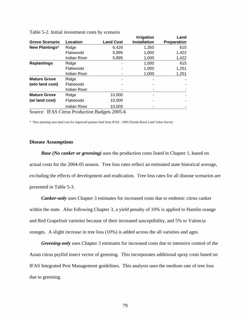
79
Table 5-2. Initial investment costs by scenario
Grove Scenario Location Land Cost Irrigation
Installation Land
Preparation
New Plantings* Ridge 6,426 1,350 615
Flatwoods 5,895 1,000 1,422
Indian River 5,895 1,000 1,422
Replantings Ridge - 1,000 615
Flatwoods - 1,000 1,251
Indian River - 1,000 1,251
Mature Grove Ridge - - -
(w/o land cost) Flatwoods - - -
Indian River - - -
Mature Grove Ridge 10,000 - -
(w/ land cost) Flatwoods 10,000 - -
Indian River 10,000 - -
Source: IFAS Citrus Production Budgets 2005-6
* New planting uses land cost for improved pasture land from IFAS - 2005 Florida Rural Land Value Survey
Disease Assumptions
Base (No canker or greening) uses the production costs listed in Chapter 1, based on
actual costs for the 2004-05 season. Tree loss rates reflect an estimated state historical average,
excluding the effects of development and eradication. Tree loss rates for all disease scenarios are
presented in Table 5-3.
Canker-only uses Chapter 3 estimates for increased costs due to endemic citrus canker
within the state. Also following Chapter 3, a yield penalty of 10% is applied to Hamlin orange
and Red Grapefruit varieties because of their increased susceptibility, and 5% to Valencia
oranges. A slight increase in tree loss (10%) is added across the all varieties and ages.
Greening-only uses Chapter 3 estimates for increased costs due to intensive control of the
Asian citrus psyllid insect vector of greening. This incorporates additional spray costs based on
IFAS Integrated Pest Management guidelines. This analysis uses the medium rate of tree loss
due to greening.
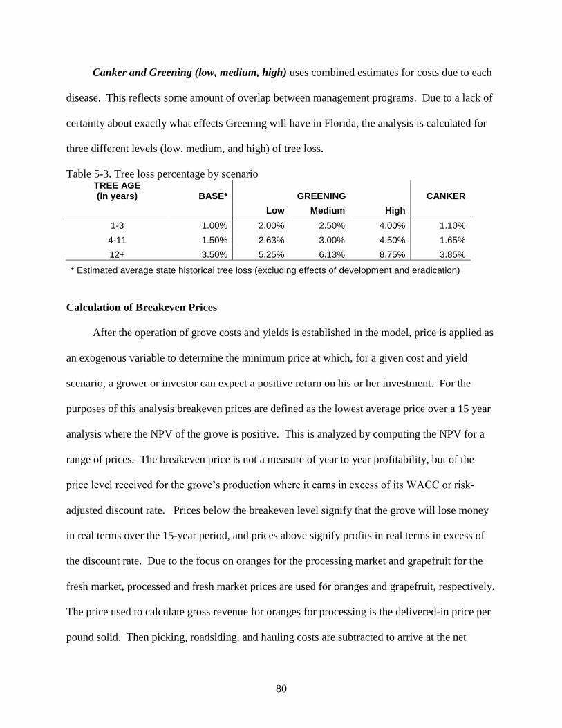
80
Canker and Greening (low, medium, high) uses combined estimates for costs due to each
disease. This reflects some amount of overlap between management programs. Due to a lack of
certainty about exactly what effects Greening will have in Florida, the analysis is calculated for
three different levels (low, medium, and high) of tree loss.
Table 5-3. Tree loss percentage by scenario TREE AGE (in years) BASE* GREENING CANKER
Low Medium High
1-3 1.00% 2.00% 2.50% 4.00% 1.10%
4-11 1.50% 2.63% 3.00% 4.50% 1.65%
12+ 3.50% 5.25% 6.13% 8.75% 3.85%
* Estimated average state historical tree loss (excluding effects of development and eradication)
Calculation of Breakeven Prices
After the operation of grove costs and yields is established in the model, price is applied as
an exogenous variable to determine the minimum price at which, for a given cost and yield
scenario, a grower or investor can expect a positive return on his or her investment. For the
purposes of this analysis breakeven prices are defined as the lowest average price over a 15 year
analysis where the NPV of the grove is positive. This is analyzed by computing the NPV for a
range of prices. The breakeven price is not a measure of year to year profitability, but of the
price level received for the grove’s production where it earns in excess of its WACC or risk-
adjusted discount rate. Prices below the breakeven level signify that the grove will lose money
in real terms over the 15-year period, and prices above signify profits in real terms in excess of
the discount rate. Due to the focus on oranges for the processing market and grapefruit for the
fresh market, processed and fresh market prices are used for oranges and grapefruit, respectively.
The price used to calculate gross revenue for oranges for processing is the delivered-in price per
pound solid. Then picking, roadsiding, and hauling costs are subtracted to arrive at the net
81
revenue of a box of oranges delivered to a processing plant. The price used to calculate revenue
for grapefruit is a combination of the on-tree price per box for fresh and processed sales. The
“on-tree price” is the value of a box of fruit already subtracted the costs of picking, roadsiding,
and hauling. Grapefruit grown for the fresh market will have a certain number of fruit graded
unfit for fresh sale (eliminated) and sent for processing into juice instead. The percentage of the
total amount of fruit delivered to the packinghouse and sent to the fresh market is referred to as
the “packout” rate, and these receive a much higher price than fruit sent for processing. The
packout rate is assumed to be 60%. On-tree fresh prices in dollars per box are reported below,
while eliminations sent for processing receive a price of $2/box in all scenarios.
Results of the Mixed-Age Grove Model – Breakeven Price Analysis
Under field conditions, citrus production is not nearly as deterministic as portrayed in this
analysis. Citrus trees are biological organisms and thus respond (sometimes unpredictably) to
changes in their environment. Climate and individual grove site characteristics have important
and widely divergent effects on production and costs. Also, there is evidence that alternate
bearing patterns exist for some varieties, and may significantly affect tree yields in a given
season. Production costs and technologies change over time and affect operating budgets.
Moreover, growers practice a range of cultural care programs, and their individual costs may be
different.
Individual growers, landowners, or investors have different asset/liability positions, tax
rates, capital gain/loss carry forwards, and risk preferences that change the dynamics and
profitability of a citrus investment. All analysis and calculations are conducted on the basis of
unleveraged cash flows before income tax in order to focus on cash flows attributable
specifically to citrus operations. Also, by excluding land value appreciation through the terminal
82
grove valuation method used, we attempt to remove distortions caused by recent surges in
Florida rural land values, and arrive at a true value for growing citrus in Florida.
The scenarios and assumptions presented attempt to illustrate important aspects of the
decision-making process faced by those involved in citrus production across Florida. Citrus is an
investment where a large upfront cost is incurred (buying and preparing the land and planting the
trees) with operating profits delayed several years until the trees become productive, and sunk
costs being recouped after that, all depending on volatile fruit prices. Due to the nature of
discounted cash flow analysis, changes in the upfront investment costs have a disproportionate
effect on a grove’s NPV. Breakeven prices for all scenarios analyzed are summarized in Table
5-4.
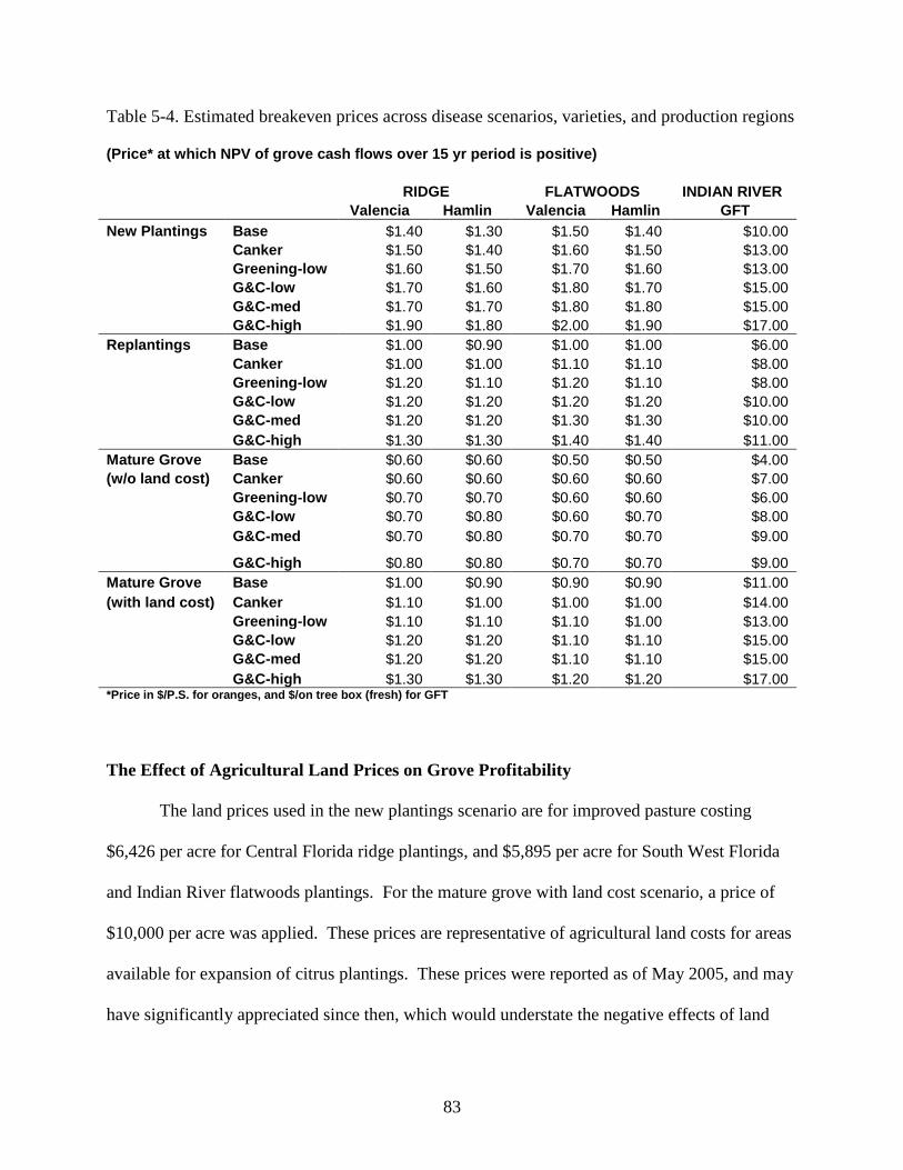
83
Table 5-4. Estimated breakeven prices across disease scenarios, varieties, and production regions
(Price* at which NPV of grove cash flows over 15 yr period is positive)
RIDGE FLATWOODS INDIAN RIVER
Valencia Hamlin Valencia Hamlin GFT
New Plantings Base $1.40 $1.30 $1.50 $1.40 $10.00
Canker $1.50 $1.40 $1.60 $1.50 $13.00
Greening-low $1.60 $1.50 $1.70 $1.60 $13.00
G&C-low $1.70 $1.60 $1.80 $1.70 $15.00
G&C-med $1.70 $1.70 $1.80 $1.80 $15.00
G&C-high $1.90 $1.80 $2.00 $1.90 $17.00
Replantings Base $1.00 $0.90 $1.00 $1.00 $6.00
Canker $1.00 $1.00 $1.10 $1.10 $8.00
Greening-low $1.20 $1.10 $1.20 $1.10 $8.00
G&C-low $1.20 $1.20 $1.20 $1.20 $10.00
G&C-med $1.20 $1.20 $1.30 $1.30 $10.00
G&C-high $1.30 $1.30 $1.40 $1.40 $11.00
Mature Grove Base $0.60 $0.60 $0.50 $0.50 $4.00
(w/o land cost) Canker $0.60 $0.60 $0.60 $0.60 $7.00
Greening-low $0.70 $0.70 $0.60 $0.60 $6.00
G&C-low $0.70 $0.80 $0.60 $0.70 $8.00
G&C-med $0.70 $0.80 $0.70 $0.70 $9.00
G&C-high $0.80 $0.80 $0.70 $0.70 $9.00
Mature Grove Base $1.00 $0.90 $0.90 $0.90 $11.00
(with land cost) Canker $1.10 $1.00 $1.00 $1.00 $14.00
Greening-low $1.10 $1.10 $1.10 $1.00 $13.00
G&C-low $1.20 $1.20 $1.10 $1.10 $15.00
G&C-med $1.20 $1.20 $1.10 $1.10 $15.00
G&C-high $1.30 $1.30 $1.20 $1.20 $17.00 *Price in $/P.S. for oranges, and $/on tree box (fresh) for GFT
The Effect of Agricultural Land Prices on Grove Profitability
The land prices used in the new plantings scenario are for improved pasture costing
$6,426 per acre for Central Florida ridge plantings, and $5,895 per acre for South West Florida
and Indian River flatwoods plantings. For the mature grove with land cost scenario, a price of
$10,000 per acre was applied. These prices are representative of agricultural land costs for areas
available for expansion of citrus plantings. These prices were reported as of May 2005, and may
have significantly appreciated since then, which would understate the negative effects of land
84
costs on new plantings. The current rural land price market in Florida constitutes a relatively
large and disproportionate upfront cost for a grower who wishes to purchase land and plant
citrus.
In reality, all citrus growers have incurred a land cost at some point, and the assumption
of zero land cost in the replanting and mature grove scenarios without land cost is not realistic.
Some portion of this land cost should be charged against the returns of a citrus investment. As in
any commercial real estate investment, many growers/landowners/investors look not only at the
income generated by the property, but also appreciation of the underlying land. Since this
analysis values only the returns associated with a citrus investment, and not land price
appreciation, these scenarios can be thought of as establishing upper and lower bounds on the
profitability of grove investment decisions facing the Florida citrus industry.
At the upper extreme, some growers/landowners/investors may evaluate a citrus grove as
an investment in isolation, and only care about the returns to the citrus operation. Therefore,
they may apply the entire land cost against the profitability of the grove. This is illustrated by
the new plantings scenario, and could represent those growers considering citrus as their primary
business. At the lower extreme, some growers/landowners/investors are purely interested in
returns from land price appreciation, and view citrus as an interim income producing activity
until they opt to realize their gains on the land. These owners would not apply any of the land
cost against the profitability of the grove, instead viewing land cost as recouped upon eventual
sale of the grove. This is illustrated by the replanting (without land cost) scenario, and could
represent investors acquiring land for future non-agricultural development. The replanting
scenario (without land cost) also includes growers who may have had sections of groves
85
eradicated due to canker, but do not have the ability to sell the area due to effects on their entire
grove.
The reality is that most people involved in growing citrus are somewhere in the middle;
neither charging the entire land cost against the citrus investment, nor expecting the entire return
on investment to come from land price appreciation. In weighing the results of this analysis, one
should view the breakeven prices for new planting and mature groves with land costs against
replanting and mature groves without land costs as a range between which one can expect
investment or planting of citrus. According to this analysis for a Valencia orange grove on the
ridge, even with the presence of endemic canker and a high rate of tree loss due to greening, a
citrus investment is profitable in the range of $1.30/P.S. (for replanting without land cost) to
$1.90/P.S. (for new planting with land cost). This range incorporates our conservative estimate
for the residual value of the grove as explained in Chapter 4.
The Effect of Canker on Grove Profitability
The change in costs from the base scenario is the greatest (+26% and +22%) for
new/replanting and a mature grove of grapefruit, respectively, because of significantly increased
spray and canker-free certification costs for fresh market citrus. The increase in costs for
new/replanting of Hamlin oranges (+11-13%) compared to Valencia oranges (+8-9%) reflects
Hamlin’s increased susceptibility to canker and required additional sprays.
Yield penalties of 10% for Hamlin oranges and grapefruit, and 5% for Valencia oranges
were incorporated into the analysis to estimate canker’s effect on per tree production, and tree
loss rates were increased 10% over the historical average across varieties to account for the
removal of infected trees. Changes in average yields due to canker are slightly higher due to the
compounded effect of the yield penalty and higher tree loss.
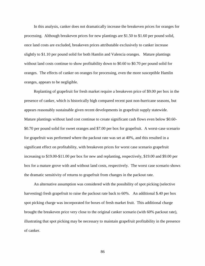
86
In this analysis, canker does not dramatically increase the breakeven prices for oranges for
processing. Although breakeven prices for new plantings are $1.50 to $1.60 per pound solid,
once land costs are excluded, breakeven prices attributable exclusively to canker increase
slightly to $1.10 per pound solid for both Hamlin and Valencia oranges. Mature plantings
without land costs continue to show profitability down to $0.60 to $0.70 per pound solid for
oranges. The effects of canker on oranges for processing, even the more susceptible Hamlin
oranges, appears to be negligible.
Replanting of grapefruit for fresh market require a breakeven price of $9.00 per box in the
presence of canker, which is historically high compared recent past non-hurricane seasons, but
appears reasonably sustainable given recent developments in grapefruit supply statewide.
Mature plantings without land cost continue to create significant cash flows even below $0.60-
$0.70 per pound solid for sweet oranges and $7.00 per box for grapefruit. A worst-case scenario
for grapefruit was performed where the packout rate was set at 40%, and this resulted in a
significant effect on profitability, with breakeven prices for worst case scenario grapefruit
increasing to $19.00-$11.00 per box for new and replanting, respectively, $19.00 and $9.00 per
box for a mature grove with and without land costs, respectively. The worst case scenario shows
the dramatic sensitivity of returns to grapefruit from changes in the packout rate.
An alternative assumption was considered with the possibility of spot picking (selective
harvesting) fresh grapefruit to raise the packout rate back to 60%. An additional $.40 per box
spot picking charge was incorporated for boxes of fresh market fruit. This additional charge
brought the breakeven price very close to the original canker scenario (with 60% packout rate),
illustrating that spot picking may be necessary to maintain grapefruit profitability in the presence
of canker.
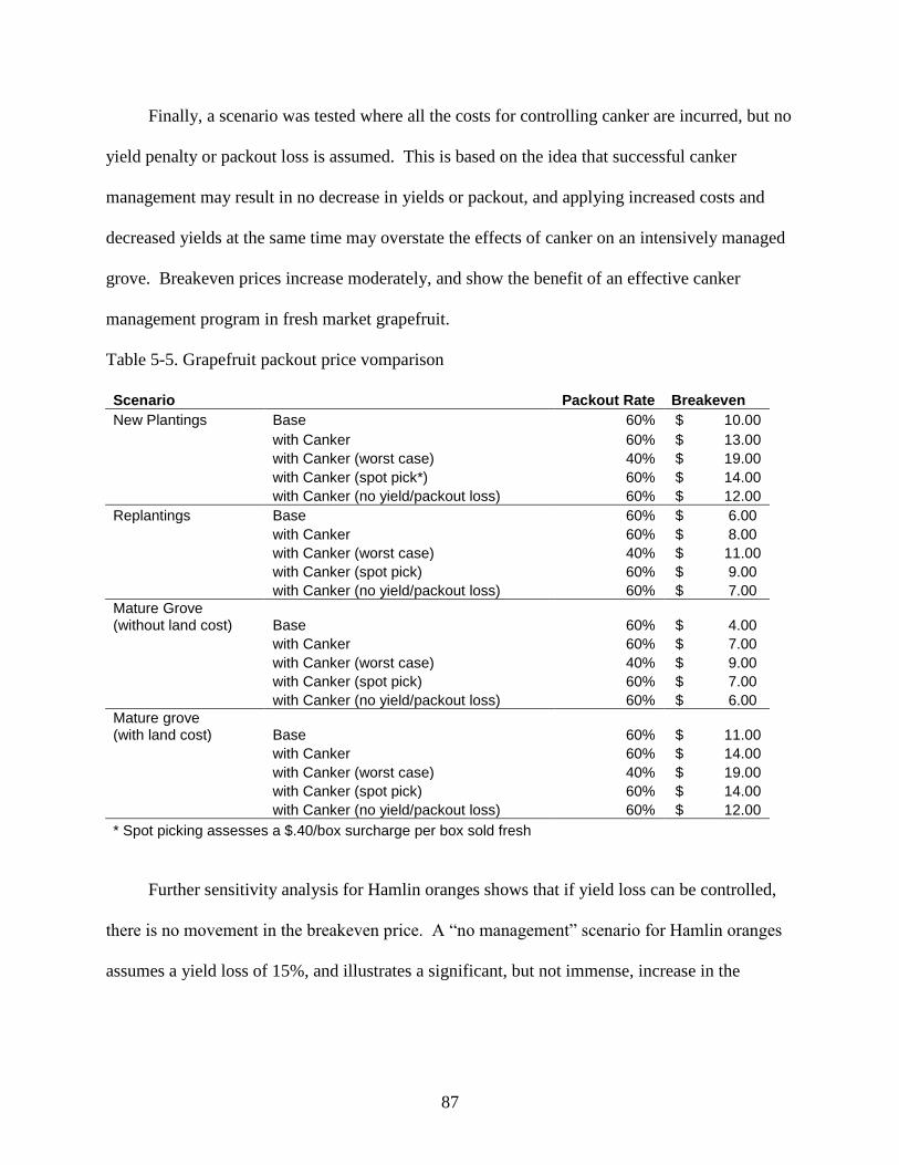
87
Finally, a scenario was tested where all the costs for controlling canker are incurred, but no
yield penalty or packout loss is assumed. This is based on the idea that successful canker
management may result in no decrease in yields or packout, and applying increased costs and
decreased yields at the same time may overstate the effects of canker on an intensively managed
grove. Breakeven prices increase moderately, and show the benefit of an effective canker
management program in fresh market grapefruit.
Table 5-5. Grapefruit packout price vomparison
Scenario Packout Rate Breakeven
New Plantings Base 60% $ 10.00
with Canker 60% $ 13.00
with Canker (worst case) 40% $ 19.00
with Canker (spot pick*) 60% $ 14.00
with Canker (no yield/packout loss) 60% $ 12.00
Replantings Base 60% $ 6.00
with Canker 60% $ 8.00
with Canker (worst case) 40% $ 11.00
with Canker (spot pick) 60% $ 9.00
with Canker (no yield/packout loss) 60% $ 7.00
Mature Grove (without land cost) Base 60% $ 4.00
with Canker 60% $ 7.00
with Canker (worst case) 40% $ 9.00
with Canker (spot pick) 60% $ 7.00
with Canker (no yield/packout loss) 60% $ 6.00
Mature grove (with land cost) Base 60% $ 11.00
with Canker 60% $ 14.00
with Canker (worst case) 40% $ 19.00
with Canker (spot pick) 60% $ 14.00
with Canker (no yield/packout loss) 60% $ 12.00
* Spot picking assesses a $.40/box surcharge per box sold fresh
Further sensitivity analysis for Hamlin oranges shows that if yield loss can be controlled,
there is no movement in the breakeven price. A “no management” scenario for Hamlin oranges
assumes a yield loss of 15%, and illustrates a significant, but not immense, increase in the
88
breakeven price. This suggests that profitability for a Hamlin grove selling to the processing
market may not be catastrophically affected by canker.
Table 5-6. Hamlin yield-loss sensitivity
Scenario Yield Loss Breakeven
New Plantings Base 0% $1.40
with Canker 10% $1.50
with Canker (no yield loss) 0% $1.40
with Canker (no management) 15% $1.60
Replantings Base 0% $1.00
with Canker 10% $1.10
with Canker (no yield loss) 0% $1.00
with Canker (no management) 15% $1.20
Mature Grove ( without land cost) Base 0% $0.50
with Canker 10% $0.60
with Canker (no yield loss) 0% $0.60
with Canker (no management) 15% $0.70
Mature grove (with land cost) Base 0% $0.90
with Canker 10% $1.00
with Canker (no yield loss) 0% $0.90
with Canker (no management) 15% $1.10
While increasing production costs and decreasing yields, especially for fresh market
grapefruit, canker in isolation appears to have a relatively small effect on the profitability of
Florida oranges for juice processing. Canker’s effect on fresh market grapefruit is also
significant and bordering on catastrophic if canker reduces packout rates. It can be supposed that
if adequate control measures are taken, and canker is not allowed to firmly establish itself in a
grove, profitability will remain mostly unchanged.
Effects of Greening on Grove Profitability
In the greening-only analysis, we assume greening increases tree loss to 2% per year for
trees from 0 to 3 years of age, 2.63% for trees aged 4-11, and 5.25% for trees 12+ years. This is
compared to the historic state-wide tree loss rate of 1%, 1.5%, and 3.5%, respectively. Psyllid
89
control, increased resetting, and field inspections for greening result in an increase in production
costs across all varieties and grove ages. Production costs for oranges increase (+32%-35%) for
new plantings/replanting and (+25%-27%) for mature plantings. Production costs for grapefruit
increase (+27%) for new planting/replanting and (+21%) for mature plantings. The difference
between new planting/replanting and mature plantings reflect the disproportionate effect of
greening on young tree loss, and the need to incur additional reset costs. However, mature
groves suffer larger reductions in average per acre yields due to the absolute increase in the loss
of older, highly productive trees.
The presence of greening appears to have a greater effect on breakeven prices compared to
canker. Breakeven prices for new plantings move into the $1.50-$1.70 per pound solid range for
oranges, and $13.00 per box for grapefruit. Breakeven prices for replanting are $1.10-$1.20 per
pound solid for oranges, and $8.00 per box for grapefruit. Breakeven prices for mature groves
without land costs are less than $.60-$.70 per pound solid for sweet oranges and $6.00 per box
for grapefruit. This indicates that while greening by itself does boost production costs
significantly, its effect on replanting and mature groves (without land costs) given current price
levels shows that citrus remains a profitable investment.
A sensitivity analysis on tree loss rates exhibit that higher tree loss rates has a small effect
on breakeven prices. Another effect of greening is that average annual tree maintenance costs
actually decline as tree loss rates increase. This result relates to the use of precision agriculture
in which greening kills older trees and reduces the amount of materials and labor required for
their maintenance, plus harvest costs decline due to reduced yields. This trend may be an artifact
of the analysis assumptions and may not reflect actual grove circumstances. Moreover,
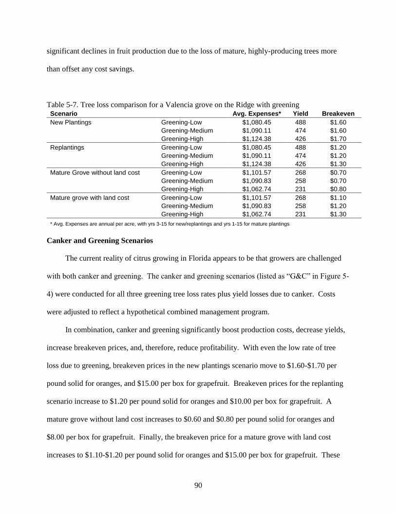
90
significant declines in fruit production due to the loss of mature, highly-producing trees more
than offset any cost savings.
Table 5-7. Tree loss comparison for a Valencia grove on the Ridge with greening Scenario Avg. Expenses* Yield Breakeven
New Plantings Greening-Low $1,080.45 488 $1.60
Greening-Medium $1,090.11 474 $1.60
Greening-High $1,124.38 426 $1.70
Replantings Greening-Low $1,080.45 488 $1.20
Greening-Medium $1,090.11 474 $1.20
Greening-High $1,124.38 426 $1.30
Mature Grove without land cost Greening-Low $1,101.57 268 $0.70
Greening-Medium $1,090.83 258 $0.70
Greening-High $1,062.74 231 $0.80
Mature grove with land cost Greening-Low $1,101.57 268 $1.10
Greening-Medium $1,090.83 258 $1.20
Greening-High $1,062.74 231 $1.30
* Avg. Expenses are annual per acre, with yrs 3-15 for new/replantings and yrs 1-15 for mature plantings
Canker and Greening Scenarios
The current reality of citrus growing in Florida appears to be that growers are challenged
with both canker and greening. The canker and greening scenarios (listed as “G&C” in Figure 5-
4) were conducted for all three greening tree loss rates plus yield losses due to canker. Costs
were adjusted to reflect a hypothetical combined management program.
In combination, canker and greening significantly boost production costs, decrease yields,
increase breakeven prices, and, therefore, reduce profitability. With even the low rate of tree
loss due to greening, breakeven prices in the new plantings scenario move to $1.60-$1.70 per
pound solid for oranges, and $15.00 per box for grapefruit. Breakeven prices for the replanting
scenario increase to $1.20 per pound solid for oranges and $10.00 per box for grapefruit. A
mature grove without land cost increases to $0.60 and $0.80 per pound solid for oranges and
$8.00 per box for grapefruit. Finally, the breakeven price for a mature grove with land cost
increases to $1.10-$1.20 per pound solid for oranges and $15.00 per box for grapefruit. These
91
prices are high by historical standards, and the possibility of achieving sustained prices above
$1.50 per pound solid for oranges or $10.00 per box for grapefruit is questionable. Therefore,
canker and greening act to decrease the profitability, especially of new plantings and mature
groves where land must be purchased at market prices.
92
CHAPTER 6
SUMMARY AND CONCLUSIONS
Given the short period that the Florida citrus industry has dealt with greening and canker, it
is too soon to conclude that the fundamental economics of growing citrus in Florida have
changed. The challenge associated with analyzing the impact of canker, greening, and increasing
rural land prices is principally the novelty of these issues to Florida growers, and a lack of
historical data regarding their effects. Any economic analysis on disease effects on grove
production must make assumptions by quantifying non-linear and highly complex biological
phenomena into monetary or production units in order to be measured. Any economic analysis
on the effects of land prices on a grove investment’s profitability is inherently tied to people’s
expectations of the value of future income from the land plus appreciation, where assumptions
must be made through the discount rate and exit capitalization rate. This analysis uses a NPV
framework to evaluate the profitability of a citrus investment, makes assumptions grounded in
actual historical data for production costs and yields, and then makes reasonable assumptions
about the monetary effects of these new challenges to Florida growers. The value of this
examination is to draw conclusions about the attractiveness of investing in citrus for the
“average” citrus grower/investor, and any changes that these new challenges may cause. From
the conclusions drawn about the economics of a citrus investment, we may be able to predict the
future entry and exit of investors in the Florida citrus industry given the behavior of production
costs and fruit prices. The limitation of this examination is the unique situation of each grower
and grove, which alters any conclusions made which are based on the grove production cost and
yield. In addition, the complex and untested nature of the assumptions used to quantify these
new challenges introduces uncertainty into the analysis and ultimate future of the Florida citrus
industry.
93
The assumptions about the consequences of a growing environment with endemic canker
and greening on grove production were made by looking at production data from other countries
and controlled scientific studies, however, the reality of what the true manifestations of these
diseases will be in the distinct ecologies of Florida and these diseases’ interaction with the
infinitely complex biological environment will take time to study and predict. Overall, the
development of new production technologies, and the experimentation and adaptation by Florida
growers to the manifestations of these diseases will be the true indicator of the long-term success
of the Florida citrus industry.
In the first outbreak of canker in Florida in 1910, anecdotal accounts relate many trees
became rapidly infected and unproductive, which led to the statewide eradication of a significant
portion of Florida citrus trees. At that time groves, however, were not irrigated, fertilizer and
pesticide technology was in its infancy, and biological research into the means of infection was
rudimentary compared to today. The assumptions made about yield loss and production cost
increases are primarily drawn from Argentina’s experience with canker, which is shares certain
similarities to Florida’s climate and environment, but has a significantly lower overall level of
production technology. Long-term studies are needed to measure the spread and virility of
infection within different Florida grove locations and by variety, the rate of decline and potential
rehabilitation of infected trees, and best practices for disease control including sprays, tree-care,
and grove sanitary controls. These will be the determinants of the ultimate economic
consequences of growing citrus in an endemic canker environment.
Greening has devastated citrus industries in Asia and Africa, but these citrus industries
were nowhere near the sophistication of Florida growers in terms of production technology, and
had little access to the resources and scientific knowledge available to the Florida citrus industry.
94
Sprays and systemic insecticides aid in the control of the citrus psyllid insect vector, and there is
a mounting body of evidence that drought and disease-stressed trees are more susceptible to
infection. Most likely, this will increase the production cost of growing citrus, however, the
Florida citrus industry is already moving towards irrigation and regular spray programs for most
commercial groves, therefore the marginal increase in production cost of controlling for greening
may be lower than the approximately 30% assumed in this analysis.
Large institutions such as the University of Florida’s Institute of Food and Agricultural
Sciences (IFAS), the USDA Agricultural Research Center at Ft. Pierce (USDA-ARS), the
Florida Department of Agriculture and Consumer Services (FDACS), and private industry are
investing significant effort into controlling and managing greening. The Florida citrus industry
should soon expect results from these research endeavors, including: the establishment of best
practices for greening control and management and new methods of biological/chemical control
of the psyllid vector. Since greening is fatal to citrus trees, if the spread of greening between and
inside groves cannot be controlled, this will have particularly negative effects on the citrus
investment because of the time frame necessary for the development and profitability of the
grove. If the average life expectancy for citrus trees is shortened to eight years (as was the case
in Thailand) the economics of growing citrus in Florida is impractical. Therefore, this author
recommends that future research efforts to determine the economic effect of greening must focus
on the probability of the spread of greening between groves and control of greening within a
grove. This will be the ultimate test of the assumptions used in this analysis.
The effect of land prices on grove profitability is more easily quantified because there
exists a market of agricultural land prices and historical information about the behavior of land
prices over time. Unfortunately, deriving an assumption for the average value of land and
95
making comparisons between citrus properties is difficult for two reasons. First, every piece of
land is unique in that it has a specific physical location which carries specific attributes such as
soil, drainage, micro-climate, and distance to packinghouses or processing plants which have a
direct impact upon the productivity and profitability of the grove. Second, land prices are
subject to people’s expectations about the future economic value derived from use or ownership
of the land. Expectations about the highest and best use of many Florida citrus groves is
changing as the state becomes more urbanized, and a large demand of non-agricultural users for
citrus growing land (particularly in the central ridge and east coast production areas) is divorcing
the value of citrus land from the value of citrus production.
This analysis attempts to quantify the value of citrus land within the net present value
framework where it is assumed that the value of the land equals the present value of the
discounted cash flows plus a future sale value (terminal grove value) at the end of the projection
period. In this analysis, the terminal grove value is derived from the built-up exit capitalization
rate method which makes it a function of citrus prices, grove production, market interest rates,
the historical volatility of citrus prices, a premium for the ownership risk and additional effort
required to manage an agricultural operation, a liquidity premium, and a cost of money
management assumed for the additional financial structure required for the operation of a citrus
investment compared to other investment options (i.e. stocks, bonds, and other financial
instruments). In this formula, the one determinant more or less common to all growers is the
market interest rate. All other premiums are subjective and specific to the preferences of each
grower/investor, and therefore lead to different expectations of grove value.
The built-up exit cap method is still based on the NPV framework and therefore the
income derived from citrus growing, however, non-agricultural demand for citrus land adds an
96
additional appreciation to the transaction price of citrus land as the potential income from non-
agricultural uses is higher than citrus, and has the effect of lowering the exit cap rate for citrus
investments. This appreciation is highly property specific and is dependent on the grove’s
potential for conversion to non-agricultural use. In this analysis, the prices derived for the citrus
exit cap rate were similar to actual market transactions from the 1999-2004 period which were
taken as a sample which excluded the effects of the strong non-agricultural demand for citrus
properties. Overall, this analysis attempts to exclude appreciation due to non-agricultural
demand, but this appreciation exists, and may be a significant component of grower/investors
subjective valuation of a citrus grove. At the time of writing, macroeconomic factors have
slowed the non-agricultural demand for citrus land, however, continued tracking of Florida
agricultural land prices, such as done through the IFAS Florida Rural Land Value Survey, is
necessary to determine whether citrus land prices will revert to being more closely correlated
with the income value of land, or a new price level is established for Florida rural land and will
persist.
In this analysis, citrus prices are treated as an exogenous variable; however, they are the
ultimate determinate of the profitability of the citrus investment. Analysis of citrus price trends
is outside the scope of this analysis, but price is the most important component of this analysis as
the effects of citrus canker, greening, and rural land prices are all compared on the basis of the
relative change in the breakeven price for the citrus investment within the NPV framework. All
results are relative to citrus prices, and the current high price environment makes the citrus
investment profitable even with significant increases in production cost, tree loss, and land
prices.
97
The economic model of perfect competition suggests that excess profits or losses are
transitory and with no barriers to entry or exit the marginal price of selling a good equals the
marginal cost of producing it, and the dynamics of production and competition in the Florida
citrus industry exhibit many similarities to this model. Within this model, the NPV of the citrus
investment can be considered a proxy for excess profit or losses, while the breakeven price
where the NPV equals zero can be considered an equilibrium point. If current prices are
expected to be above this breakeven price, then one can expect citrus acreage to expand until the
additional supply forces prices down to their equilibrium level, and vice versa in the case of price
expectations below the current breakeven price. In the real world, many factors conspire to
complicate and cloud this fundamental relationship, such as: imperfect information, different
subjective price expectations, different risk expectations (as transmitted through the discount
rate), different cost structures, lags in supply response, changes in demand, foreign competition,
and personal preferences.
In attempting to construct an average return to the citrus investment, we can begin to draw
conclusions about the current and future prospects for the Florida citrus industry. This analysis
finds that current price levels (as of Fall 2007) around $1.75 per pound solid, if sustained, make
many of the scenarios examined profitable, even in the presence of canker, greening, and high
land prices. The major question remaining is if the current high price environment is sustainable
and citrus has established a new higher equilibrium price. In the long run, canker, greening, and
higher citrus land prices should act to force up the cost of production, and therefore the
equilibrium price, however, more research is needed to determine whether other factors,
principally US consumer demand for citrus products and Brazilian citrus production costs will
allow the price to remain higher.
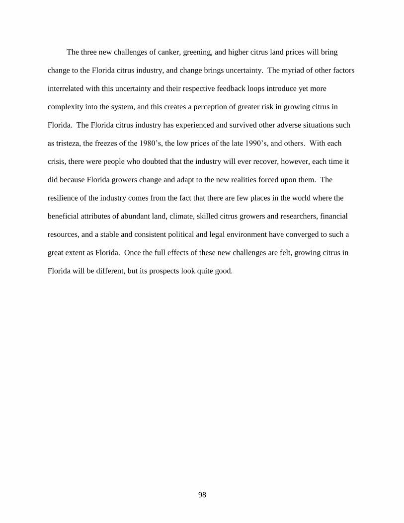
98
The three new challenges of canker, greening, and higher citrus land prices will bring
change to the Florida citrus industry, and change brings uncertainty. The myriad of other factors
interrelated with this uncertainty and their respective feedback loops introduce yet more
complexity into the system, and this creates a perception of greater risk in growing citrus in
Florida. The Florida citrus industry has experienced and survived other adverse situations such
as tristeza, the freezes of the 1980’s, the low prices of the late 1990’s, and others. With each
crisis, there were people who doubted that the industry will ever recover, however, each time it
did because Florida growers change and adapt to the new realities forced upon them. The
resilience of the industry comes from the fact that there are few places in the world where the
beneficial attributes of abundant land, climate, skilled citrus growers and researchers, financial
resources, and a stable and consistent political and legal environment have converged to such a
great extent as Florida. Once the full effects of these new challenges are felt, growing citrus in
Florida will be different, but its prospects look quite good.
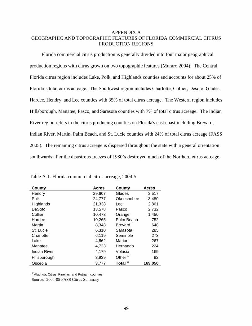
99
APPENDIX A
GEOGRAPHIC AND TOPOGRAPHIC FEATURES OF FLORIDA COMMERCIAL CITRUS
PRODUCTION REGIONS
Florida commercial citrus production is generally divided into four major geographical
production regions with citrus grown on two topographic features (Muraro 2004). The Central
Florida citrus region includes Lake, Polk, and Highlands counties and accounts for about 25% of
Florida’s total citrus acreage. The Southwest region includes Charlotte, Collier, Desoto, Glades,
Hardee, Hendry, and Lee counties with 35% of total citrus acreage. The Western region includes
Hillsborough, Manatee, Pasco, and Sarasota counties with 7% of total citrus acreage. The Indian
River region refers to the citrus producing counties on Florida's east coast including Brevard,
Indian River, Martin, Palm Beach, and St. Lucie counties with 24% of total citrus acreage (FASS
2005). The remaining citrus acreage is dispersed throughout the state with a general orientation
southwards after the disastrous freezes of 1980’s destroyed much of the Northern citrus acreage.
Table A-1. Florida commercial citrus acreage, 2004-5
County Acres County Acres
Hendry 29,607 Glades 3,517
Polk 24,777 Okeechobee 3,480
Highlands 21,338 Lee 2,861
DeSoto 13,578 Pasco 2,732
Collier 10,478 Orange 1,450
Hardee 10,265 Palm Beach 752
Martin 8,348 Brevard 648
St. Lucie 6,310 Sarasota 285
Charlotte 6,119 Seminole 273
Lake 4,862 Marion 267
Manatee 4,723 Hernando 224
Indian River 4,179 Volusia 169
Hillsborough 3,939 Other 1/ 92
Osceola 3,777 Total 2/ 169,050
1/
Alachua, Citrus, Pinellas, and Putnam counties
Source: 2004-05 FASS Citrus Summary
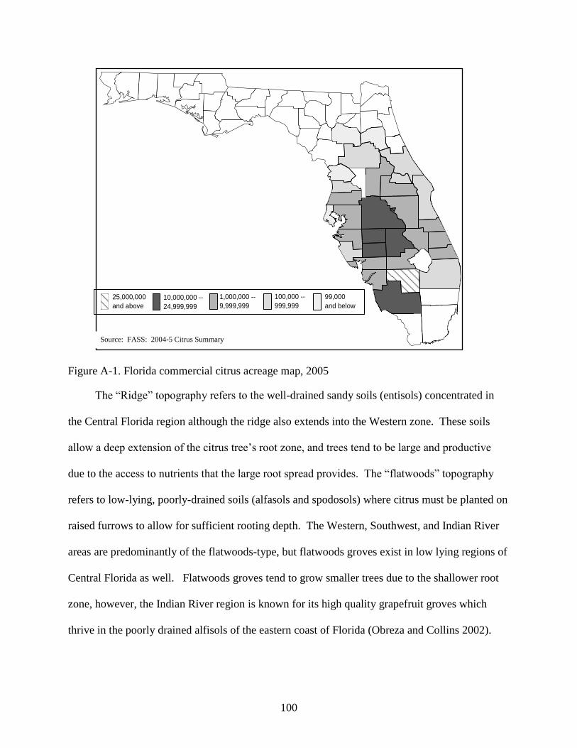
100
1,000,000 --
9,999,999
100,000 --
999,999
10,000,000 --
24,999,999
25,000,000
and above
99,000
and below
Figure A-1. Florida commercial citrus acreage map, 2005
The “Ridge” topography refers to the well-drained sandy soils (entisols) concentrated in
the Central Florida region although the ridge also extends into the Western zone. These soils
allow a deep extension of the citrus tree’s root zone, and trees tend to be large and productive
due to the access to nutrients that the large root spread provides. The “flatwoods” topography
refers to low-lying, poorly-drained soils (alfasols and spodosols) where citrus must be planted on
raised furrows to allow for sufficient rooting depth. The Western, Southwest, and Indian River
areas are predominantly of the flatwoods-type, but flatwoods groves exist in low lying regions of
Central Florida as well. Flatwoods groves tend to grow smaller trees due to the shallower root
zone, however, the Indian River region is known for its high quality grapefruit groves which
thrive in the poorly drained alfisols of the eastern coast of Florida (Obreza and Collins 2002).
Source: FASS: 2004-5 Citrus Summary
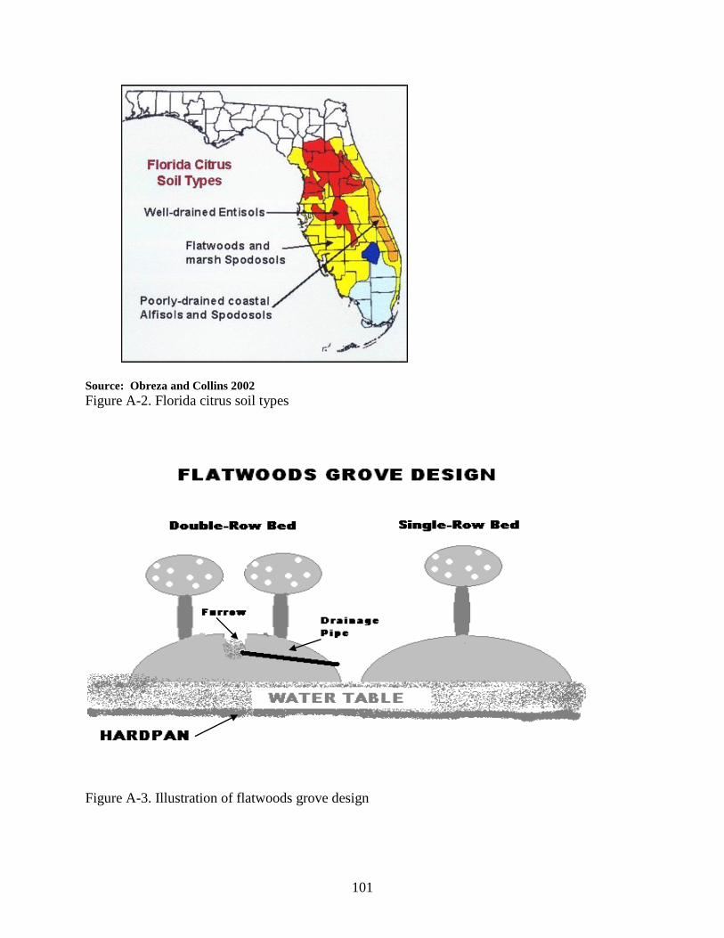
101
Source: Obreza and Collins 2002
Figure A-2. Florida citrus soil types
Figure A-3. Illustration of flatwoods grove design
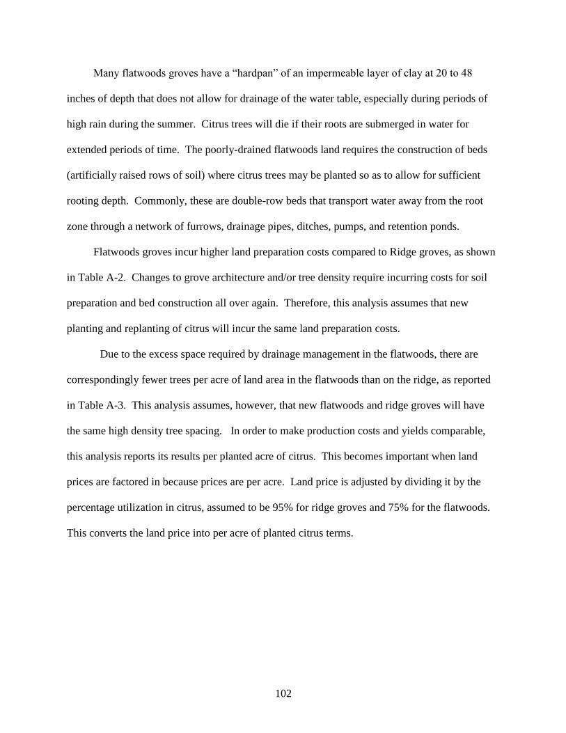
102
Many flatwoods groves have a “hardpan” of an impermeable layer of clay at 20 to 48
inches of depth that does not allow for drainage of the water table, especially during periods of
high rain during the summer. Citrus trees will die if their roots are submerged in water for
extended periods of time. The poorly-drained flatwoods land requires the construction of beds
(artificially raised rows of soil) where citrus trees may be planted so as to allow for sufficient
rooting depth. Commonly, these are double-row beds that transport water away from the root
zone through a network of furrows, drainage pipes, ditches, pumps, and retention ponds.
Flatwoods groves incur higher land preparation costs compared to Ridge groves, as shown
in Table A-2. Changes to grove architecture and/or tree density require incurring costs for soil
preparation and bed construction all over again. Therefore, this analysis assumes that new
planting and replanting of citrus will incur the same land preparation costs.
Due to the excess space required by drainage management in the flatwoods, there are
correspondingly fewer trees per acre of land area in the flatwoods than on the ridge, as reported
in Table A-3. This analysis assumes, however, that new flatwoods and ridge groves will have
the same high density tree spacing. In order to make production costs and yields comparable,
this analysis reports its results per planted acre of citrus. This becomes important when land
prices are factored in because prices are per acre. Land price is adjusted by dividing it by the
percentage utilization in citrus, assumed to be 95% for ridge groves and 75% for the flatwoods.
This converts the land price into per acre of planted citrus terms.
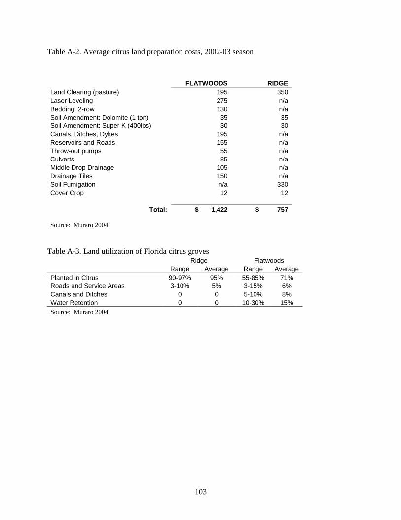
103
Table A-2. Average citrus land preparation costs, 2002-03 season
FLATWOODS RIDGE
Land Clearing (pasture) 195 350
Laser Leveling 275 n/a
Bedding: 2-row 130 n/a
Soil Amendment: Dolomite (1 ton) 35 35
Soil Amendment: Super K (400lbs) 30 30
Canals, Ditches, Dykes 195 n/a
Reservoirs and Roads 155 n/a
Throw-out pumps 55 n/a
Culverts 85 n/a
Middle Drop Drainage 105 n/a
Drainage Tiles 150 n/a
Soil Fumigation n/a 330
Cover Crop 12 12
Total: $ 1,422 $ 757
Source: Muraro 2004
Table A-3. Land utilization of Florida citrus groves Ridge Flatwoods
Range Average Range Average
Planted in Citrus 90-97% 95% 55-85% 71%
Roads and Service Areas 3-10% 5% 3-15% 6%
Canals and Ditches 0 0 5-10% 8%
Water Retention 0 0 10-30% 15%
Source: Muraro 2004
104
APPENDIX B
PARAMETERS USED IN THE ANALYSIS
In this appendix, input data used in the grove investment analysis is presented. This
includes establishment cost for new plantings, reset costs, grove maintenance costs for both a
newly established and mature grove. This data is presented in Tables B-1 through B-4
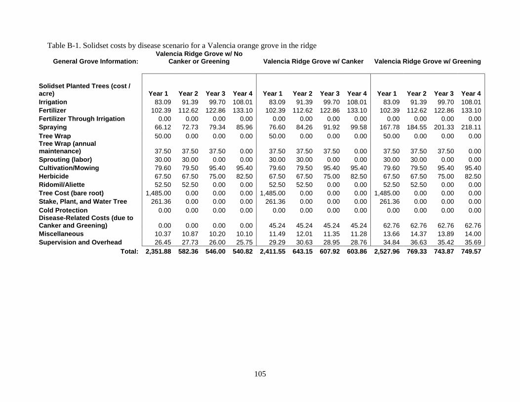
105
Table B-1. Solidset costs by disease scenario for a Valencia orange grove in the ridge
General Grove Information: Valencia Ridge Grove w/ No
Canker or Greening Valencia Ridge Grove w/ Canker Valencia Ridge Grove w/ Greening
Solidset Planted Trees (cost / acre) Year 1 Year 2 Year 3 Year 4 Year 1 Year 2 Year 3 Year 4 Year 1
Year 2
Year 3
Year 4
Irrigation 83.09 91.39 99.70 108.01 83.09 91.39 99.70 108.01 83.09 91.39 99.70 108.01
Fertilizer 102.39 112.62 122.86 133.10 102.39 112.62 122.86 133.10 102.39 112.62 122.86 133.10
Fertilizer Through Irrigation 0.00 0.00 0.00 0.00 0.00 0.00 0.00 0.00 0.00 0.00 0.00 0.00
Spraying 66.12 72.73 79.34 85.96 76.60 84.26 91.92 99.58 167.78 184.55 201.33 218.11
Tree Wrap 50.00 0.00 0.00 0.00 50.00 0.00 0.00 0.00 50.00 0.00 0.00 0.00 Tree Wrap (annual maintenance) 37.50 37.50 37.50 0.00 37.50 37.50 37.50 0.00 37.50 37.50 37.50 0.00
Sprouting (labor) 30.00 30.00 0.00 0.00 30.00 30.00 0.00 0.00 30.00 30.00 0.00 0.00
Cultivation/Mowing 79.60 79.50 95.40 95.40 79.60 79.50 95.40 95.40 79.60 79.50 95.40 95.40
Herbicide 67.50 67.50 75.00 82.50 67.50 67.50 75.00 82.50 67.50 67.50 75.00 82.50
Ridomil/Aliette 52.50 52.50 0.00 0.00 52.50 52.50 0.00 0.00 52.50 52.50 0.00 0.00
Tree Cost (bare root) 1,485.00 0.00 0.00 0.00 1,485.00 0.00 0.00 0.00 1,485.00 0.00 0.00 0.00
Stake, Plant, and Water Tree 261.36 0.00 0.00 0.00 261.36 0.00 0.00 0.00 261.36 0.00 0.00 0.00
Cold Protection 0.00 0.00 0.00 0.00 0.00 0.00 0.00 0.00 0.00 0.00 0.00 0.00 Disease-Related Costs (due to Canker and Greening) 0.00 0.00 0.00 0.00 45.24 45.24 45.24 45.24 62.76 62.76 62.76 62.76
Miscellaneous 10.37 10.87 10.20 10.10 11.49 12.01 11.35 11.28 13.66 14.37 13.89 14.00
Supervision and Overhead 26.45 27.73 26.00 25.75 29.29 30.63 28.95 28.76 34.84 36.63 35.42 35.69
Total: 2,351.88 582.36 546.00 540.82 2,411.55 643.15 607.92 603.86 2,527.96 769.33 743.87 749.57
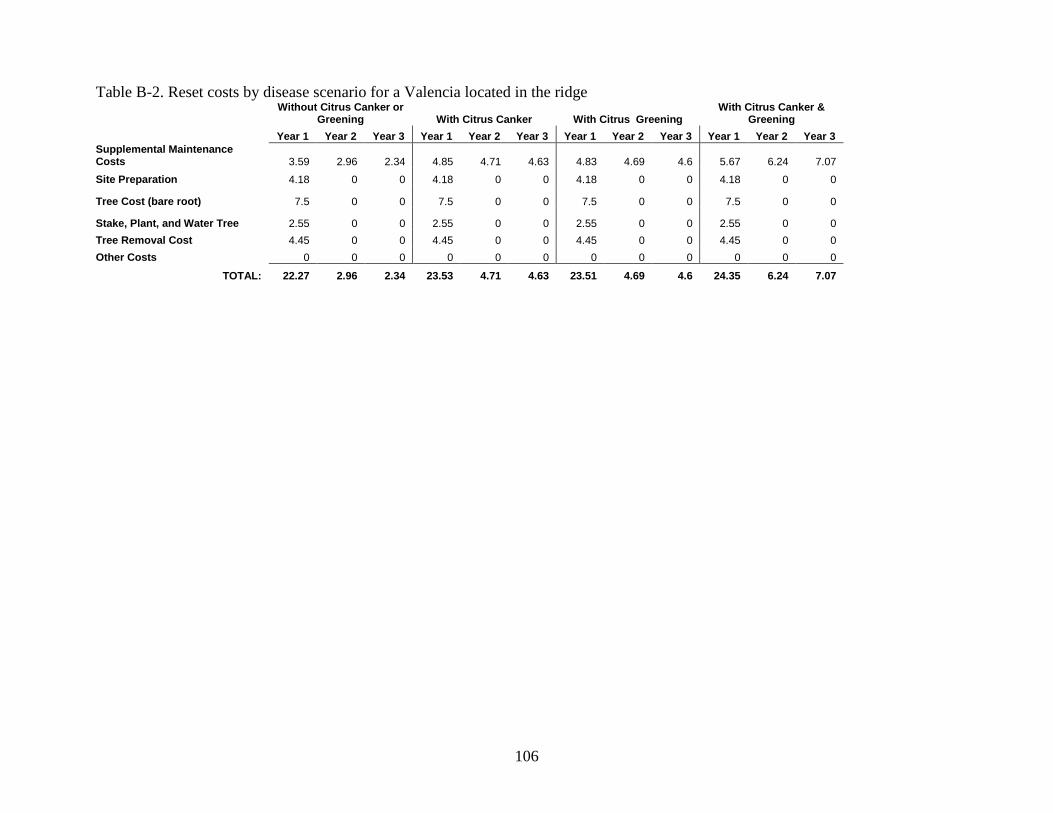
106
Table B-2. Reset costs by disease scenario for a Valencia located in the ridge
Without Citrus Canker or
Greening With Citrus Canker With Citrus Greening With Citrus Canker &
Greening
Year 1 Year 2 Year 3 Year 1 Year 2 Year 3 Year 1 Year 2 Year 3 Year 1 Year 2 Year 3
Supplemental Maintenance Costs 3.59 2.96 2.34 4.85 4.71 4.63 4.83 4.69 4.6 5.67 6.24 7.07
Site Preparation 4.18 0 0 4.18 0 0 4.18 0 0 4.18 0 0
Tree Cost (bare root) 7.5 0 0 7.5 0 0 7.5 0 0 7.5 0 0
Stake, Plant, and Water Tree 2.55 0 0 2.55 0 0 2.55 0 0 2.55 0 0
Tree Removal Cost 4.45 0 0 4.45 0 0 4.45 0 0 4.45 0 0
Other Costs 0 0 0 0 0 0 0 0 0 0 0 0
TOTAL: 22.27 2.96 2.34 23.53 4.71 4.63 23.51 4.69 4.6 24.35 6.24 7.07
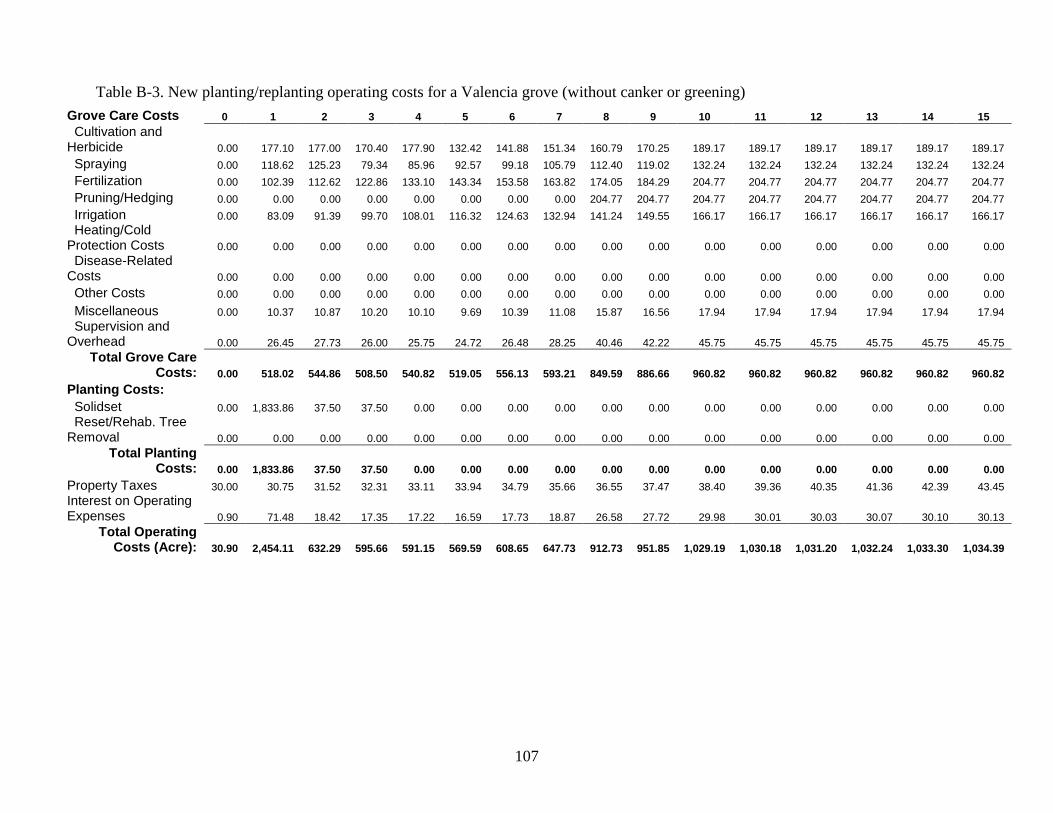
107
Table B-3. New planting/replanting operating costs for a Valencia grove (without canker or greening)
Grove Care Costs 0 1 2 3 4 5 6 7 8 9 10 11 12 13 14 15
Cultivation and Herbicide 0.00 177.10 177.00 170.40 177.90 132.42 141.88 151.34 160.79 170.25 189.17 189.17 189.17 189.17 189.17 189.17
Spraying 0.00 118.62 125.23 79.34 85.96 92.57 99.18 105.79 112.40 119.02 132.24 132.24 132.24 132.24 132.24 132.24
Fertilization 0.00 102.39 112.62 122.86 133.10 143.34 153.58 163.82 174.05 184.29 204.77 204.77 204.77 204.77 204.77 204.77
Pruning/Hedging 0.00 0.00 0.00 0.00 0.00 0.00 0.00 0.00 204.77 204.77 204.77 204.77 204.77 204.77 204.77 204.77
Irrigation 0.00 83.09 91.39 99.70 108.01 116.32 124.63 132.94 141.24 149.55 166.17 166.17 166.17 166.17 166.17 166.17
Heating/Cold Protection Costs 0.00 0.00 0.00 0.00 0.00 0.00 0.00 0.00 0.00 0.00 0.00 0.00 0.00 0.00 0.00 0.00
Disease-Related Costs 0.00 0.00 0.00 0.00 0.00 0.00 0.00 0.00 0.00 0.00 0.00 0.00 0.00 0.00 0.00 0.00
Other Costs 0.00 0.00 0.00 0.00 0.00 0.00 0.00 0.00 0.00 0.00 0.00 0.00 0.00 0.00 0.00 0.00
Miscellaneous 0.00 10.37 10.87 10.20 10.10 9.69 10.39 11.08 15.87 16.56 17.94 17.94 17.94 17.94 17.94 17.94
Supervision and Overhead 0.00 26.45 27.73 26.00 25.75 24.72 26.48 28.25 40.46 42.22 45.75 45.75 45.75 45.75 45.75 45.75
Total Grove Care Costs: 0.00 518.02 544.86 508.50 540.82 519.05 556.13 593.21 849.59 886.66 960.82 960.82 960.82 960.82 960.82 960.82
Planting Costs:
Solidset 0.00 1,833.86 37.50 37.50 0.00 0.00 0.00 0.00 0.00 0.00 0.00 0.00 0.00 0.00 0.00 0.00
Reset/Rehab. Tree Removal 0.00 0.00 0.00 0.00 0.00 0.00 0.00 0.00 0.00 0.00 0.00 0.00 0.00 0.00 0.00 0.00
Total Planting Costs: 0.00 1,833.86 37.50 37.50 0.00 0.00 0.00 0.00 0.00 0.00 0.00 0.00 0.00 0.00 0.00 0.00
Property Taxes 30.00 30.75 31.52 32.31 33.11 33.94 34.79 35.66 36.55 37.47 38.40 39.36 40.35 41.36 42.39 43.45
Interest on Operating Expenses 0.90 71.48 18.42 17.35 17.22 16.59 17.73 18.87 26.58 27.72 29.98 30.01 30.03 30.07 30.10 30.13
Total Operating Costs (Acre): 30.90 2,454.11 632.29 595.66 591.15 569.59 608.65 647.73 912.73 951.85 1,029.19 1,030.18 1,031.20 1,032.24 1,033.30 1,034.39
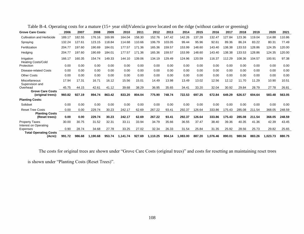
108
Table B-4. Operating costs for a mature (15+ year old)Valencia grove located on the ridge (without canker or greening)
Grove Care Costs: 2006 2007 2008 2009 2010 2011 2012 2013 2014 2015 2016 2017 2018 2019 2020 2021
Cultivation and Herbicide 189.17 182.55 176.16 169.99 164.04 158.30 152.76 147.42 142.26 137.28 132.47 127.84 123.36 119.04 114.88 110.86
Spraying 132.24 127.61 123.15 118.84 114.68 110.66 106.79 103.05 99.44 95.96 92.61 89.36 86.24 83.22 80.31 77.49
Fertilization 204.77 197.60 190.69 184.01 177.57 171.36 165.36 159.57 153.99 148.60 143.40 138.38 133.53 128.86 124.35 120.00
Hedging 204.77 197.60 190.69 184.01 177.57 171.36 165.36 159.57 153.99 148.60 143.40 138.38 133.53 128.86 124.35 120.00
Irrigation 166.17 160.35 154.74 149.33 144.10 139.06 134.19 129.49 124.96 120.59 116.37 112.29 108.36 104.57 100.91 97.38 Heating Costs/Cold Protection 0.00 0.00 0.00 0.00 0.00 0.00 0.00 0.00 0.00 0.00 0.00 0.00 0.00 0.00 0.00 0.00
Disease-related Costs 0.00 0.00 0.00 0.00 0.00 0.00 0.00 0.00 0.00 0.00 0.00 0.00 0.00 0.00 0.00 0.00
Other Costs 0.00 0.00 0.00 0.00 0.00 0.00 0.00 0.00 0.00 0.00 0.00 0.00 0.00 0.00 0.00 0.00
Miscellaneous 17.94 17.31 16.71 16.12 15.56 15.01 14.49 13.98 13.49 13.02 12.56 12.12 11.70 11.29 10.90 10.51 Supervision and Overhead 45.75 44.15 42.61 41.12 39.68 38.29 36.95 35.65 34.41 33.20 32.04 30.92 29.84 28.79 27.78 26.81
Grove Care Costs (original trees): 960.82 927.19 894.74 863.42 833.20 804.04 775.90 748.74 722.53 697.25 672.84 649.29 626.57 604.64 583.48 563.05
Planting Costs:
Solidset 0.00 0.00 0.00 0.00 0.00 0.00 0.00 0.00 0.00 0.00 0.00 0.00 0.00 0.00 0.00 0.00
Reset Tree Costs 0.00 0.00 229.74 30.23 242.17 62.69 267.22 93.41 292.37 126.64 333.86 175.43 285.08 211.54 368.05 248.59
Planting Costs (Reset trees): 0.00 0.00 229.74 30.23 242.17 62.69 267.22 93.41 292.37 126.64 333.86 175.43 285.08 211.54 368.05 248.59
Property Taxes 30.00 30.75 31.52 32.31 33.11 33.94 34.79 35.66 36.55 37.47 38.40 39.36 40.35 41.36 42.39 43.45 Interest on Operating Expenses 0.90 28.74 34.68 27.78 33.25 27.02 32.34 26.33 31.54 25.84 31.35 25.92 28.56 25.73 29.82 25.65
Total Operating Costs (Acre): 991.72 986.68 1,190.68 953.74 1,141.74 927.69 1,110.25 904.14 1,083.00 887.20 1,076.46 890.01 980.56 883.26 1,023.73 880.75
The costs for original trees are shown under “Grove Care Costs (original trees)” and costs for resetting an maintaining reset trees
is shown under “Planting Costs (Reset Trees)”.
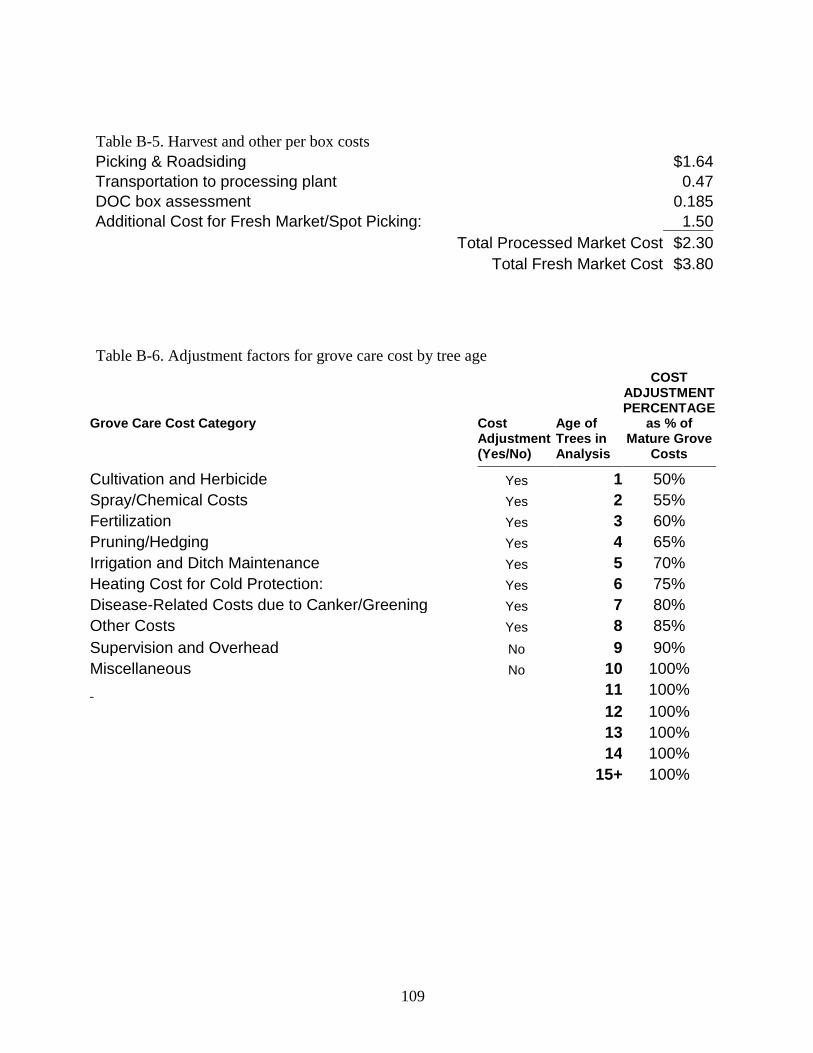
109
Table B-5. Harvest and other per box costs
Picking & Roadsiding $1.64
Transportation to processing plant 0.47
DOC box assessment 0.185
Additional Cost for Fresh Market/Spot Picking: 1.50
Total Processed Market Cost $2.30
Total Fresh Market Cost $3.80
Table B-6. Adjustment factors for grove care cost by tree age
COST ADJUSTMENT PERCENTAGE
Grove Care Cost Category Cost Adjustment (Yes/No)
Age of Trees in Analysis
as % of Mature Grove
Costs
Cultivation and Herbicide Yes 1 50%
Spray/Chemical Costs Yes 2 55%
Fertilization Yes 3 60%
Pruning/Hedging Yes 4 65%
Irrigation and Ditch Maintenance Yes 5 70%
Heating Cost for Cold Protection: Yes 6 75%
Disease-Related Costs due to Canker/Greening Yes 7 80%
Other Costs Yes 8 85%
Supervision and Overhead No 9 90%
Miscellaneous No 10 100%
11 100%
12 100%
13 100% 14 100% 15+ 100%
110
Table B-7. Annual irrigation expense (ridge/flatwoods comparison) ($/Acre)
Variable Operating Expense (Diesel) 59.44
Annual Maintenance 50.17
Fixed-Depreciation Expense (non-cash) 56.56
"Ridge" Total: 166.17
(Additional for Flatwoods)
Clean Ditches (Weed Control) 14.19
Ditch and Canal Maintenance 15.06
Water Control (Pump water
in/out of Ditches and Canals) 13.21
"Flatwoods" and “Indian River” Total: 208.63
Source: 2004-5 IFAS Citrus Production Budgets
Table B-8. Average per acre citrus land preparation costs (ridge/flatwoods comparison) FLATWOODS RIDGE
Land Clearing (pasture) 195 350
Laser Leveling 275 n/a
Bedding: 2-row 130 n/a
Soil Amendment: Dolomite (1 ton) 35 35
Soil Amendment: Super K (400lbs) 30 30
Canals, Ditches, Dykes 195 n/a
Reservoirs and Roads 155 n/a
Throw-out pumps 55 n/a
Culverts 85 n/a
Middle Drop Drainage 105 n/a
Drainage Tiles 150 n/a
Soil Fumigation n/a 330
Cover Crop 12 12
Total: 1,422 757
Source: 2004-5 IFAS Citrus Production Budgets
Table B-9. Property tax levy for top five citrus producing counties, 2003
County Millage Rate A.P.R. (%)*
Polk 17.322 1.73%
Hendry 21.062 2.11%
St. Lucie 20.855 2.09%
Highlands 18.477 1.85% *A.P.R. is annual percentage rate of the millage rate converted into a percent
source: Hodges et al. 2003
111
Table B-10. Property tax analysis assumptions
Mature Grove New Planting/Replanting
Market Value* $ 5,721.00 $ 2,934.00
Assessment Value ($/acre) $ 3,600.00 $ 1,550.00
Millage Rate ($/$1000 of value) 19.5 19.5
Effective A.P.R.(%) 1.95% 1.95%
Annual Property Tax ($/acre) $ 70.20 $ 30.23
* Market value is 2003 value for Central Florida mature oranges and improved pasture for new/replanting
Source: Hodges et al. (2003) and 2003 IFAS Florida Rural Land Value Survey
Table B-11. USDA average yields by variety and production district, 1999-2004 average
VALENCIA ORANGES
3-5 Years 6-8 Years 9-13 Years 14-23 Years 24+ Years
Indian River 0.8 1.3 1.75 2.03 2.68
North&Central 1.03 1.72 2.45 3.59 5.67
Western 1.5 2.22 2.89 3.28 4.26
Southern 0.94 1.67 2.1 2.45 4.07
Statewide 1.09 1.73 2.28 2.83 4.33
EARLY/MIDSEASON ORANGES
3-5 Years 6-8 Years 9-13 Years 14-23 Years 24+ Years
Indian River 0.65 1.51 1.87 2.49 3.03
North&Central 1.36 2.3 3.46 4.75 6.4
Western 1.27 1.74 3.33 4.58 5.32
Southern 1.14 1.9 2.82 3.62 4.11
Statewide 1.16 1.96 3.1 4.13 4.94
COLORED GRAPEFRUIT
3-5 Years 6-8 Years 9-13 Years 14-23 Years 24+ Years
Indian River 1.41 2.18 3.14 4.37 5.01
North&Central 2.67 3.2 4.68 7.35 8.36
Western 2.43 1.64 4.27 2.68 7.18
Southern 2.96 4.1 4.11 4.72 5.67
Statewide 1.86 2.8 3.62 4.58 5.24
Source: 2003-4 Florida Citrus Summary
112
Table B-12. Rootstock study for Valencia oranges on ridge and flatwoods sites
AVON PARK (145 Trees/Acre) INDIANTOWN (102 Trees/Acre)
SWINGLE CARRIZO SWINGLE CARRIZO
SEASON TREE AGE Box/Tree P.S./Box Box/Tree P.S./Box Box/Tree P.S./Box Box/Tree P.S./Box
1980/81 1 0.00 0.00 0.00 0.00 0.00 0.00 0.00 0.00
1981/82 2 0.00 0.00 0.00 0.00 0.00 0.00 0.00 0.00
1982/83 3 0.24 6.56 0.26 6.57 0.00 0.00 0.00 0.00
1983/84 4 0.97 4.96 1.26 4.81 0.20 5.03 0.30 4.63
1984/85 5 1.04 5.92 1.57 5.82 0.40 5.03 0.80 4.63
1985/86 6 1.36 6.04 1.85 5.70 1.00 5.03 1.70 4.63
1986/87 7 1.58 6.14 2.93 6.22 1.60 7.68 2.20 8.04
1987/88 8 1.69 6.26 1.95 6.22 2.20 6.89 3.00 6.75
1988/89 9 3.25 5.98 5.62 5.89 3.60 5.94 4.60 6.21
1989/90 10 2.67 6.51 2.98 6.06 2.10 7.05 4.00 7.30
1990/91 11 4.06 6.54 6.00 6.44 3.00 7.15 4.60 7.60
1991/92 12 3.89 6.59 4.59 6.30 2.30 7.65 4.00 7.45
1992/93 13 3.75 6.56 5.65 6.37 4.50 6.94 6.70 6.69
1993/94 14 4.01 7.65 7.22 6.92 4.70 7.01 6.40 7.08
1994/95 15 3.91 7.18 6.53 6.78 3.00 6.77 5.30 6.91
Source: Dr. William Castle, IFAS Lake Alfred CREC
Table B-13. Fruit and juice yield by variety used in the analysis
Hamlin Orange Valencia Orange Colored
Grapefruit
Spacing: 22' x 10' 22' x 10' 25' x 13'
Trees/Acre: 198 198 134
Tree Boxes P.S. Boxes P.S. Boxes
Age Per Tree Per Tree Per Tree Per Tree Per Tree
1 0.00 0.00 0.00 0.00 0.00 2 0.00 0.00 0.00 0.00 0.00
3 0.55 5.00 0.46 5.00 0.68 4 0.91 5.25 0.77 5.50 1.14 5 1.28 5.50 1.08 6.00 1.60
6 1.73 6.00 1.47 6.50 2.17 7 2.19 6.25 1.85 7.00 2.73 8 2.55 6.25 2.16 7.00 3.19 9 2.92 6.25 2.47 7.00 3.65 10 3.28 6.25 2.78 7.00 4.10
11 3.61 6.25 3.06 7.00 4.51 12 3.61 6.25 3.06 7.00 4.51 13 3.61 6.25 3.06 7.00 4.51 14 3.61 6.25 3.06 7.00 4.51 15 3.61 6.25 3.06 7.00 4.51
113
Table B-14. Mature grove production costs with canker by production region
RIDGE FLATWOODS
VALENCIA HAMLIN VALENCIA HAMLIN GFT
Cultivation and Herbicide 189.17 189.17 189.17 189.17 189.17
Spray Program 132.24 132.24 141.19 141.19 383.17
Fertilization 204.77 204.77 204.77 204.77 157.00
Pruning 40.06 40.06 40.06 40.06 52.13
Irrigation and Ditch Maintenance 166.17 166.17 208.63 208.63 208.63
Miscellaneous 14.65 14.65 15.68 15.68 19.80
Supervision and Overhead 36.62 36.62 39.19 39.19 49.51
Water-drainage Tax - - - - 60.00
Total Grove Care (before canker) 783.68 783.68 838.69 838.69 1,119.41
Additional Disease Related Costs Canker Field Inspections 17.52 17.52 17.52 17.52 17.52
Additional Spray Program 20.96 57.12 12.01 48.17 35.26
Citrus Canker Decontamination Costs 27.72 27.72 27.72 27.72 27.72
Yearly Cost to Establish & Maintenance for Windbreak
- - - - 11.47
DPI Fresh Market Citrus Certification Costs*
- - - - 60.00
Additional Packhouse Certification Costs*
- - - - 40.50
Additional Supervision/Misc. Costs 4.63 7.17 4.01 6.54 13.47
Total Grove Care (after greening) 854.51 893.20 899.94 938.64 1,325.35
% Change from Base 9% 14% 7% 12% 18%
* Only incurred for fresh market fruit once trees reach commerical production age
114
Table B-15. Mature grove production costs with greening by production region
RIDGE FLATWOODS
VALENCIA HAMLIN VALENCIA HAMLIN GFT
Cultivation and Herbicide 189.17 189.17 189.17 189.17 189.17
Spray Program 132.24 132.24 141.19 141.19 383.17
Fertilization 204.77 204.77 204.77 204.77 157.00
Pruning 40.06 40.06 40.06 40.06 52.13
Irrigation and Ditch Maintenance 166.17 166.17 208.63 208.63 208.63
Miscellaneous 14.65 14.65 15.68 15.68 19.80
Supervision and Overhead 36.62 36.62 39.19 39.19 49.51
Water-drainage Tax - - - - 60.00
Total Grove Care (before greening) 783.68 783.68 838.69 838.69 1,119.41
Additional Disease Related Costs
Greening Field Inspections 35.04 35.04 35.04 35.04 35.04
Additional Spray Program 203.31 203.31 194.36 194.36 156.74 Additional Supervision/Misc. Costs 16.68 16.68 16.06 16.06 13.42
Total Grove Care (after greening) 1,038.71 1,038.71 1,084.15 1,084.15 1,324.61
% Change from Base 33% 33% 29% 29% 18%
115
Table B-16. Mature grove production costs with canker and greening
RIDGE FLATWOODS
VALENCIA HAMLIN VALENCIA HAMLIN GFT
Cultivation and Herbicide 189.17 189.17 189.17 189.17 189.17
Spray Program 132.24 132.24 141.19 141.19 383.17
Fertilization 204.77 204.77 204.77 204.77 157.00
Pruning 40.06 40.06 40.06 40.06 52.13
Irrigation and Ditch Maintenance 166.17 166.17 208.63 208.63 208.63
Miscellaneous 14.65 14.65 15.68 15.68 19.80
Supervision and Overhead 36.62 36.62 39.19 39.19 49.51
Water-drainage Tax - - - - 60.00 Total Grove Care (before canker & greening)
783.68 783.68 838.69 838.69 1,119.41
Additional Disease Related Costs Canker/Greening Field Inspections 35.04 35.04 35.04 35.04 35.04 Additional Spray Program 203.31 203.31 194.36 194.36 156.74
Citrus Canker Decontamination Costs 27.72 27.72 27.72 27.72 27.72
Yearly Cost to Establish & Maintenance for Windbreak
- - - - 11.47
DPI Fresh Market Citrus Certification Costs*
- - - - 60.00
Additional Packhouse Certification Costs*
- - - - 40.50
Additional Supervision/Misc. Costs 18.62 18.62 18.00 18.00 23.20
Total Grove Care (after greening) 1,068.37 1,068.37 1,113.81 1,113.81 1,474.08
% Change from Base 36% 36% 33% 33% 32%
* Only incurred for fresh market fruit once trees reach commercial production age
116
Table B-17. Spray schedule and costs by variety and disease scenario
Base Canker Greening Canker & Greening
Type/Purpose Oranges* GFT Valencia Hamlin GFT Oranges* GFT Valencia Hamlin GFT
Winter-Early Spring 118.63 118.63 118.63 118.63 118.63
Systemic Insecticide (Temik/Admire)
Psyllid control
Spring-Post Bloom (at first flush) 99.58 36.16 36.16 36.16 36.16 36.16
Oil/Copper
Rust mite/Leafminer/Fungicide
Spring-Post Bloom (3-weeks after petal fall) 83.43 37.86 54.5 54.5 54.5 54.5 54.5 54.5 54.5 54.5
Copper/Micronutrients/Lorsban
Leafminer/Rust mite/ Scale
Spring-Post Bloom (6-weeks after petal fall) 37.86 59.06 59.06 59.06
Copper/Micromite
Scab/Melanose/Rust mite
Summer (late May) 96.6 109.14 109.14 109.14
Oil/Miticide
Rust mite/Scale
Summer (late May/early June) 53.63 53.82 49.35 49.35 49.35 49.35 49.35 49.35 49.35 49.35
Copper/Oil/Miticide
Rust mite/Scale/Fungicide
Summer (early July/ mid August) 49.35 49.35 49.35 70.69 70.69 70.69 70.69 70.69
Oil/Copper/Lorsban/Micronut.
Rust mite/Scale/Fungicide/Psyllid
Fall (mid November) 57.46 60.87 42.38 42.38 42.38 42.38 42.38
Vendex or Danitol
Rust mite/psyllid control
TOTAL ($/acre) 137.06 383.18 153.20 189.36 418.43 335.55 539.91 335.55 371.71 539.91
* Oranges not separated by variety because of identical spray programs. All orange costs representative of ridge
source: IFAS 2004-5 Citrus Production Budgets adjusted by Ronald Muraro for recommended spray programs by disease
117
APPENDIX C
SELECTED RESULTS
Results from various scenarios are shown in Tables C-1 through C-6.
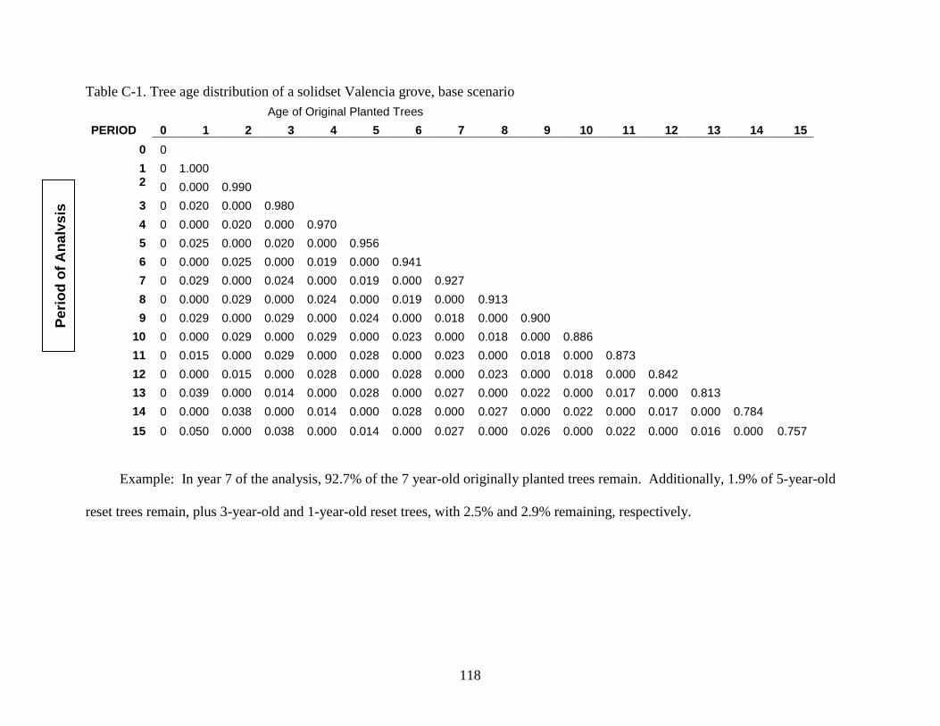
118
Table C-1. Tree age distribution of a solidset Valencia grove, base scenario
Age of Original Planted Trees
PERIOD 0 1 2 3 4 5 6 7 8 9 10 11 12 13 14 15
0 0
1 0 1.000 2 0 0.000 0.990
3 0 0.020 0.000 0.980
4 0 0.000 0.020 0.000 0.970
5 0 0.025 0.000 0.020 0.000 0.956
6 0 0.000 0.025 0.000 0.019 0.000 0.941
7 0 0.029 0.000 0.024 0.000 0.019 0.000 0.927
8 0 0.000 0.029 0.000 0.024 0.000 0.019 0.000 0.913
9 0 0.029 0.000 0.029 0.000 0.024 0.000 0.018 0.000 0.900
10 0 0.000 0.029 0.000 0.029 0.000 0.023 0.000 0.018 0.000 0.886
11 0 0.015 0.000 0.029 0.000 0.028 0.000 0.023 0.000 0.018 0.000 0.873
12 0 0.000 0.015 0.000 0.028 0.000 0.028 0.000 0.023 0.000 0.018 0.000 0.842
13 0 0.039 0.000 0.014 0.000 0.028 0.000 0.027 0.000 0.022 0.000 0.017 0.000 0.813
14 0 0.000 0.038 0.000 0.014 0.000 0.028 0.000 0.027 0.000 0.022 0.000 0.017 0.000 0.784
15 0 0.050 0.000 0.038 0.000 0.014 0.000 0.027 0.000 0.026 0.000 0.022 0.000 0.016 0.000 0.757
Example: In year 7 of the analysis, 92.7% of the 7 year-old originally planted trees remain. Additionally, 1.9% of 5-year-old
reset trees remain, plus 3-year-old and 1-year-old reset trees, with 2.5% and 2.9% remaining, respectively.
Pe
rio
d o
f A
na
lys
is
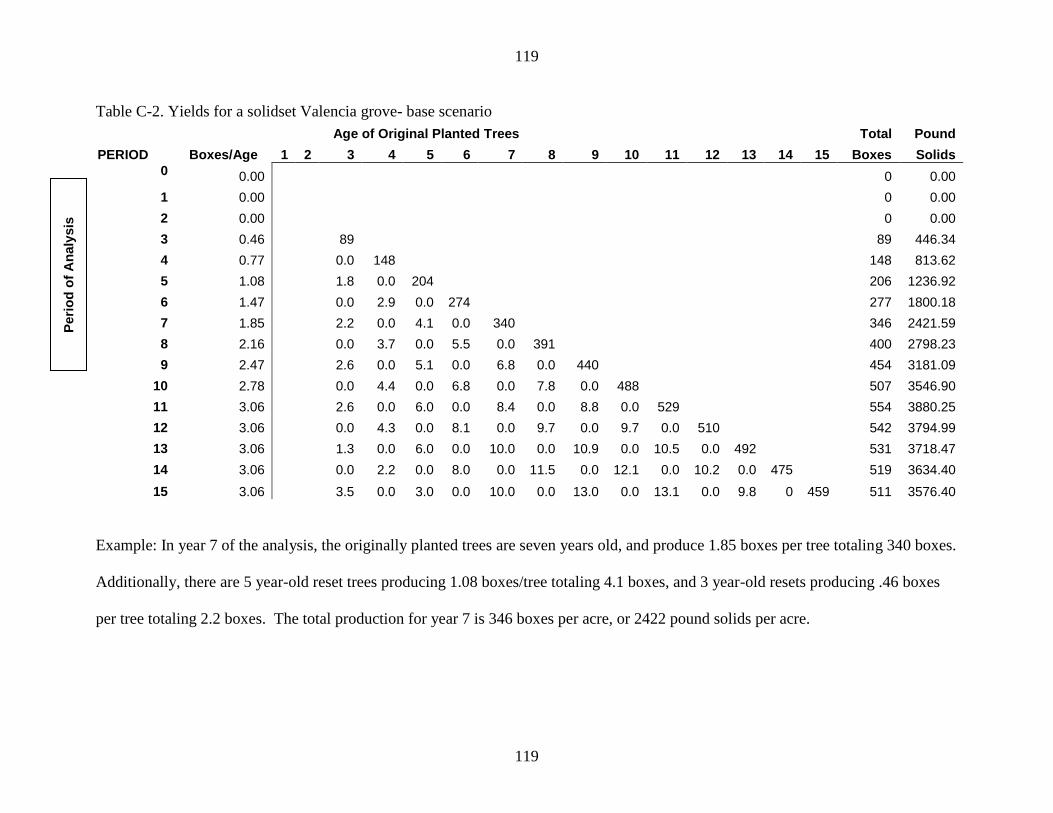
119
119
Table C-2. Yields for a solidset Valencia grove- base scenario
Age of Original Planted Trees Total Pound
PERIOD Boxes/Age 1 2 3 4 5 6 7 8 9 10 11 12 13 14 15 Boxes Solids
0 0.00 0 0.00
1 0.00 0 0.00
2 0.00 0 0.00
3 0.46 89 89 446.34
4 0.77 0.0 148 148 813.62
5 1.08 1.8 0.0 204 206 1236.92
6 1.47 0.0 2.9 0.0 274 277 1800.18
7 1.85 2.2 0.0 4.1 0.0 340 346 2421.59
8 2.16 0.0 3.7 0.0 5.5 0.0 391 400 2798.23
9 2.47 2.6 0.0 5.1 0.0 6.8 0.0 440 454 3181.09
10 2.78 0.0 4.4 0.0 6.8 0.0 7.8 0.0 488 507 3546.90
11 3.06 2.6 0.0 6.0 0.0 8.4 0.0 8.8 0.0 529 554 3880.25
12 3.06 0.0 4.3 0.0 8.1 0.0 9.7 0.0 9.7 0.0 510 542 3794.99
13 3.06 1.3 0.0 6.0 0.0 10.0 0.0 10.9 0.0 10.5 0.0 492 531 3718.47
14 3.06 0.0 2.2 0.0 8.0 0.0 11.5 0.0 12.1 0.0 10.2 0.0 475 519 3634.40
15 3.06 3.5 0.0 3.0 0.0 10.0 0.0 13.0 0.0 13.1 0.0 9.8 0 459 511 3576.40
Example: In year 7 of the analysis, the originally planted trees are seven years old, and produce 1.85 boxes per tree totaling 340 boxes.
Additionally, there are 5 year-old reset trees producing 1.08 boxes/tree totaling 4.1 boxes, and 3 year-old resets producing .46 boxes
per tree totaling 2.2 boxes. The total production for year 7 is 346 boxes per acre, or 2422 pound solids per acre.
Peri
od
of
An
aly
sis
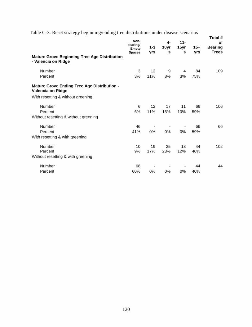
120
Table C-3. Reset strategy beginning/ending tree distributions under disease scenarios
Non-bearing/
Empty Spaces
1-3 yrs
4-10yr
s
11-15yr
s 15+ yrs
Total # of
Bearing Trees
Mature Grove Beginning Tree Age Distribution - Valencia on Ridge
Number
3
12
9
4
84
109
Percent 3% 11% 8% 3% 75%
Mature Grove Ending Tree Age Distribution - Valencia on Ridge
With resetting & without greening
Number
6
12
17
11
66
106
Percent 6% 11% 15% 10% 59%
Without resetting & without greening
Number
46
-
-
-
66
66
Percent 41% 0% 0% 0% 59%
With resetting & with greening
Number
10
19
25
13
44
102 Percent 9% 17% 23% 12% 40%
Without resetting & with greening
Number
68
-
-
-
44
44
Percent 60% 0% 0% 0% 40%
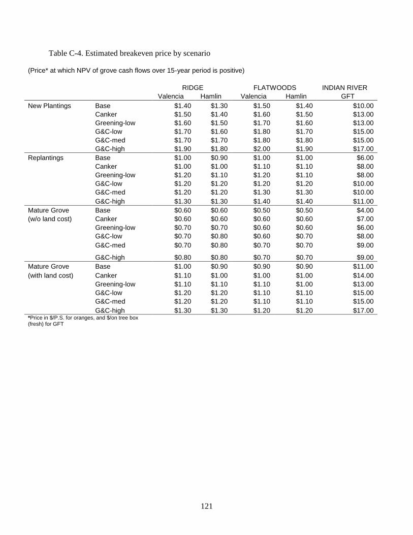
121
Table C-4. Estimated breakeven price by scenario
(Price* at which NPV of grove cash flows over 15-year period is positive)
RIDGE FLATWOODS INDIAN RIVER
Valencia Hamlin Valencia Hamlin GFT
New Plantings Base $1.40 $1.30 $1.50 $1.40 $10.00
Canker $1.50 $1.40 $1.60 $1.50 $13.00
Greening-low $1.60 $1.50 $1.70 $1.60 $13.00
G&C-low $1.70 $1.60 $1.80 $1.70 $15.00
G&C-med $1.70 $1.70 $1.80 $1.80 $15.00
G&C-high $1.90 $1.80 $2.00 $1.90 $17.00
Replantings Base $1.00 $0.90 $1.00 $1.00 $6.00
Canker $1.00 $1.00 $1.10 $1.10 $8.00
Greening-low $1.20 $1.10 $1.20 $1.10 $8.00
G&C-low $1.20 $1.20 $1.20 $1.20 $10.00
G&C-med $1.20 $1.20 $1.30 $1.30 $10.00
G&C-high $1.30 $1.30 $1.40 $1.40 $11.00
Mature Grove Base $0.60 $0.60 $0.50 $0.50 $4.00
(w/o land cost) Canker $0.60 $0.60 $0.60 $0.60 $7.00
Greening-low $0.70 $0.70 $0.60 $0.60 $6.00
G&C-low $0.70 $0.80 $0.60 $0.70 $8.00
G&C-med $0.70 $0.80 $0.70 $0.70 $9.00
G&C-high $0.80 $0.80 $0.70 $0.70 $9.00
Mature Grove Base $1.00 $0.90 $0.90 $0.90 $11.00
(with land cost) Canker $1.10 $1.00 $1.00 $1.00 $14.00
Greening-low $1.10 $1.10 $1.10 $1.00 $13.00
G&C-low $1.20 $1.20 $1.10 $1.10 $15.00
G&C-med $1.20 $1.20 $1.10 $1.10 $15.00
G&C-high $1.30 $1.30 $1.20 $1.20 $17.00 *Price in $/P.S. for oranges, and $/on tree box (fresh) for GFT
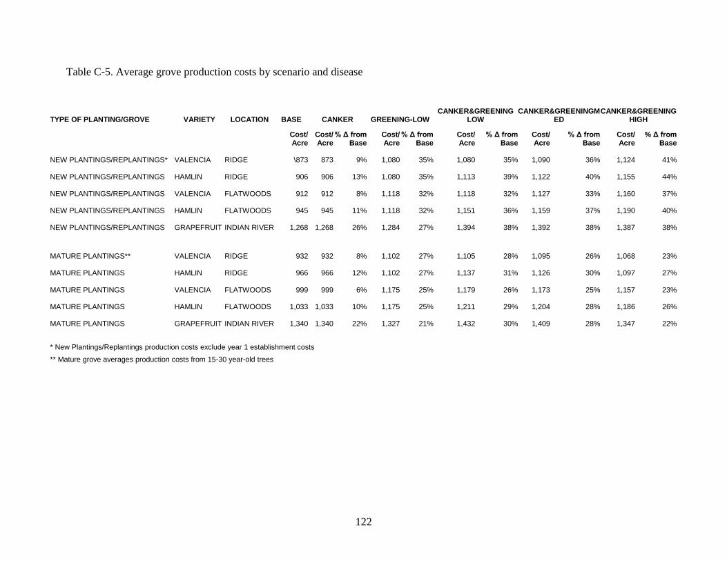
122
Table C-5. Average grove production costs by scenario and disease
TYPE OF PLANTING/GROVE VARIETY LOCATION BASE CANKER GREENING-LOW
CANKER&GREENING
LOW CANKER&GREENINGM
ED CANKER&GREENING
HIGH
Cost/ Acre
Cost/ Acre
% Δ from Base
Cost/ Acre
% Δ from Base
Cost/ Acre
% Δ from Base
Cost/ Acre
% Δ from Base
Cost/ Acre
% Δ from Base
NEW PLANTINGS/REPLANTINGS* VALENCIA RIDGE
\873
873 9% 1,080 35%
1,080 35%
1,090 36%
1,124 41%
NEW PLANTINGS/REPLANTINGS HAMLIN RIDGE
906
906 13% 1,080 35%
1,113 39%
1,122 40%
1,155 44%
NEW PLANTINGS/REPLANTINGS VALENCIA FLATWOODS
912
912 8% 1,118 32%
1,118 32%
1,127 33%
1,160 37%
NEW PLANTINGS/REPLANTINGS HAMLIN FLATWOODS
945
945 11% 1,118 32%
1,151 36%
1,159 37%
1,190 40%
NEW PLANTINGS/REPLANTINGS GRAPEFRUIT INDIAN RIVER
1,268
1,268 26% 1,284 27%
1,394 38%
1,392 38%
1,387 38%
MATURE PLANTINGS** VALENCIA RIDGE
932
932 8% 1,102 27%
1,105 28%
1,095 26%
1,068 23%
MATURE PLANTINGS HAMLIN RIDGE
966
966 12% 1,102 27%
1,137 31%
1,126 30%
1,097 27%
MATURE PLANTINGS VALENCIA FLATWOODS
999
999 6% 1,175 25%
1,179 26%
1,173 25%
1,157 23%
MATURE PLANTINGS HAMLIN FLATWOODS
1,033
1,033 10% 1,175 25%
1,211 29%
1,204 28%
1,186 26%
MATURE PLANTINGS GRAPEFRUIT INDIAN RIVER
1,340
1,340 22% 1,327 21%
1,432 30%
1,409 28%
1,347 22%
* New Plantings/Replantings production costs exclude year 1 establishment costs
** Mature grove averages production costs from 15-30 year-old trees
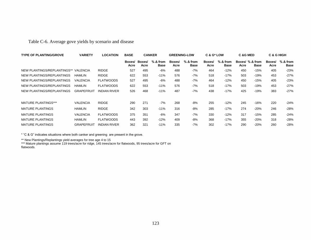
123
Table C-6. Average gove yields by scenario and disease
TYPE OF PLANTING/GROVE VARIETY LOCATION BASE CANKER GREENING-LOW
C & G* LOW C &G MED C & G HIGH
Boxes/
Acre Boxes/
Acre % Δ from
Base Boxes/
Acre % Δ from
Base Boxes/
Acre % Δ from
Base Boxes/
Acre % Δ from
Base Boxes/
Acre % Δ from
Base
NEW PLANTINGS/REPLANTINGS** VALENCIA RIDGE 527 495 -6% 488 -7% 464 -12% 450 -15% 405 -23%
NEW PLANTINGS/REPLANTINGS HAMLIN RIDGE 622 553 -11% 576 -7% 518 -17% 503 -19% 453 -27%
NEW PLANTINGS/REPLANTINGS VALENCIA FLATWOODS 527 495 -6% 488 -7% 464 -12% 450 -15% 405 -23%
NEW PLANTINGS/REPLANTINGS HAMLIN FLATWOODS 622 553 -11% 576 -7% 518 -17% 503 -19% 453 -27%
NEW PLANTINGS/REPLANTINGS GRAPEFRUIT INDIAN RIVER 526 468 -11% 487 -7% 438 -17% 425 -19% 383 -27%
MATURE PLANTINGS*** VALENCIA RIDGE 290 271 -7% 268 -8% 255 -12% 245 -16% 220 -24%
MATURE PLANTINGS HAMLIN RIDGE 342 303 -11% 316 -8% 285 -17% 274 -20% 246 -28%
MATURE PLANTINGS VALENCIA FLATWOODS 375 351 -6% 347 -7% 330 -12% 317 -15% 285 -24%
MATURE PLANTINGS HAMLIN FLATWOODS 443 392 -12% 409 -8% 368 -17% 355 -20% 318 -28%
MATURE PLANTINGS GRAPEFRUIT INDIAN RIVER 362 321 -11% 335 -7% 302 -17% 290 -20% 260 -28%
* “C & G” indicates situations where both canker and greening are present in the grove.
** New Plantings/Replantings yield averages for tree age 4 to 15 *** Mature plantings assume 119 trees/acre for ridge, 145 trees/acre for flatwoods, 95 trees/acre for GFT on flatwoods.
124
LIST OF REFERENCES
American Institute of Real Estate Appraisers. The Appraisal of Rural Property. Chicago:
American Institute of Real Estate Appraisers 1983.
Animal and Plant Health Services (APHIS). “Greening Survey Program Update: March 16th
,
2006”. http://www.aphis.usda.gov/ppq/ep/citrus_greening/pdf_files/update3-16-06.pdf
The Appraisal Institute. The Appraisal of Real Estate (12th
edition). Chicago: The Appraisal
Institute 2001.
Boscolo, M. and J.R. Vincent. “Promoting Better Logging Practices in Tropical Forests: A
Simulation Analysis of Alternative Regulations”. Land Economics. v. 76, no. 1 (2000).
pp. 1-14.
Brealey, R.A. and S.C. Meyers. Principles of Corporate Finance (7th
edition). Boston:
McGraw Hill 2003.
Buitendag, C.H. and L.A. Von Broembsen. “Living with Citrus Greening in South Africa”.
Minutes of 12th
Annual International Organization of Citrus Virologists (IOCV)
Conference. (1995) pp. 269-275.
Buongiorno, J. and B.R. Michie. “A Matrix Model of Uneven-Aged Forest Management”.
Forest Science. 26(1980):609-25.
Castle, William T. “10 year Rootstock Trials at Avon Park and Indiantown.” Citrus Education
and Research Center. University of Florida, Lake Alfred, FL 1994
Chen, C. “Ecology of the Insect Vectors of Citrus Systemic Diseases and Their Control in
Taiwan”. Proceedings of a Regional Workshop on Management of Banana and Ctirus
Through the Use of Disease-Free Planting Planting Materials. Davo City, Philippines.
October 1998.
Florida Agricultural Statistics Service. Citrus Summary, various issues . Orlando, FL
Florida Department of Agriculture and Consumer Services: “USDA Determines Citrus Canker
Eradication Program Not Feasible.” Department Press Release 01-11-2006a.
Florida Department of Agriculture and Consumer Services. “Comprehensive Report on Citrus
Canker Eradication Program in Florida.” Department Press Release 01-14-2006b.
Gottwald, T. R. and X. Sun, T. Riley, J.H. Graham, F. Ferrandino. and E. L. Taylor. “Geo-
referenced Spatiotemporal Analysis of the Urban Citrus Canker Epidemic in Florida”.
Phytopathology. 92(2002a):361-377.
125
Gottwald, T. R., J.H. Graham, and T.S. Schubert. “Citrus Canker: The Pathogen and Its Impact”.
Online. Plant Health Progress doi:10.1094/PHP-2002-0812-01-RV. 2002b.)
Graham, J.R. and C.R. Harevy. “The Theory and Practice of Corporate Finance: Evidence from
the Field”. Journal of Financial Economics. v. 60 (2001). pp. 187-223.
Heppner, J.B. “Citrus Leafminer”. IFAS EDIS: EENY038. 2003.
Hodges,A. W.D. Mulkey, R.P. Muraro, and T.H. Spreen. “County Property Values and Tax
Impacts of Florida's Citrus Industry.” IFAS EDIS: FE437. 2003.
Jackson, L.K. “Citrus Reset Management.” IFAS EDIS: HS142, 1994.
Jackson, L.K. and F. Davies. Citrus Growing in Florida-4th
Edition. Gainesville : University
Press of Florida, 1999
Ke, C. and C.F. Xu. “Successful Integrated Management of Huanglongbing Disease in Several
Farms of Guandong and Fujian by Combined Early Eradication with Targeted Insecticide
Spraying”. Proceedings of 4th
International Asia Pacific Conference on Citrus
Rehabilitation. Chiang Mai, Thailand. 1990. pp. 145-148.
Keith, Thomas. “Applying DCF Analysis to Land in Transition”. The Appraisal Journal.
59(1991): 458-70.
Leite Jr., R. P., and S.K. Mohan. “Integrated Management of the Citrus Bacterial Canker
Disease Caused by Xanthomonas campestris pv. citri in the State of Paraná, Brazil”.
Crop Protection 9(1990):3-7.
McCoy, C.W., H. N. Nigg, L.W. Timmer, S.H. Futch, and M.E. Rogers. “2006 Florida Citrus
Pest Management Guide: Use of Pesticides in Citrus IPM”. IFAS EDIS: CG035, 2005
Moss, C.B., R.N. Weldon, and R.P. Muraro. “The Impact of Risk on the Discount Rate for
Different Citrus Varities”. Agribusiness. 7 (1991): 327-38.
Muraro, R.P. “Ten Year Budget Analysis for Rehabilitation of Freeze-Damaged Citrus Groves”.
University of Florida, Food and Resource Economics Department Staff Paper No. 270,
January 1985.
Muraro, R.P. “Farm Real Estate Valuation”. University of Florida, Institute of Food and
Agricultural Sciences Circular: 333 (March 1989).
Muraro, R.P., F.M. Roka, and R.E. Rouse. “Budgeting Costs and Returns for Southwest Florida
Citrus Production 2004-5.” IFAS EDIS: FE631, 2006a.
Muraro, R.P. and J.W. Hebb. “Budgeting Costs and Returns for Indian River Citrus Production
2004-5.” IFAS EDIS: FE630, 2006b.
126
Muraro, R.P., F.M. Roka, and R.E. Rouse. “Budgeting Costs and Returns for Central Florida
Citrus Production 2004-5.” IFAS EDIS: FE629, 2006c.
Muraro, R.P. Lake Alfred Interview 2/21/2006. Lake Alfred Citrus Education and Research
Center 2006d.
Muraro, R.P., F.M. Roka, and R.E. Rouse. “Budgeting Costs and Returns for Southwest Florida
Citrus Production 2003-4.” IFAS EDIS: FE528, 2005a.
Muraro, R.P. and J.W. Hebb. “Budgeting Costs and Returns for Indian River Citrus Production
2003-4.” IFAS EDIS: FE527, 2005b.
Muraro, R.P., W.G. Hartt, and W.C. Oswalt. “Budgeting Costs and Returns for Central Citrus
Production 2003-4.” IFAS EDIS: FE526, 2005c.
Muraro, R.P. and S. Futch. Lake Alfred Interview 10/6/2005. Citrus Education and Research
Center , Lake Alfred, FL, 2005.
Muraro, R.P., J.W. Hebb, and E.W. Stover. “Budgeting Costs and Returns for Indian River
Citrus Production 2002-3.” IFAS EDIS: FE433, 2004.
Muraro, R.P. and W.C. Oswalt. “Budgeting Costs and Returns for Central Florida Citrus
Production 2002-3.” IFAS EDIS: FE432, 2004.
Muraro, R.P., F.M. Roka, and R.E. Rouse. “Budgeting Costs and Returns for Southwest Florida
Citrus Production 2002-3.” IFAS EDIS: FE434, 2004.
Muraro, R.P. and F.M. Roka. “Citrus Reset Analysis.” IFAS EDIS:FE365, 2003.
Muraro, R.P., F.M. Roka and T.H. Spreen. “Grower Costs of Having Citrus Canker in Florida”.
IFAS EDIS: FE286, 2001.
Muraro, R.P., and W.S. Castle. “Resetting and replanting options in Florida citrus groves and the
financial consequences.” Proceedings of the Florida State Horticulture Society 109: 128-
131. 1996.
Mongi Z., T. A. Obreza and R. Koo. “Irrigation, Nutrition, and Citrus Fruit Quality.” IFAS
EDIS: SL207, 2003.
Morgan, K.T. and E.A. Hanlon. “Improving Citrus Nitrogen Uptake Efficiency: Understanding
Citrus Nitrogen Requirements.” IFAS EDIS: SL240, 2006.
Obreza, T.A. and M. E. Collins. “Common Soils Used for Citrus Production in Florida.” IFAS
EDIS: SL193, 2002.
127
Parsons, L.R. and W. Wheaton. “Tree Density, Hedging, and Topping.” IFAS EDIS: HS1026.
2006.
Parsons, L.R. and B.J. Boman. “Microsprinkler Irrigation for Cold Protection of Florida Citrus”.
IFAS EDIS: HS931, 2003.
Reynolds, J.E. and A. Deas. “Florida Agricultural Land Values Increase: 2000 Survey Results.”
IFAS EDIS: FE214, 2000.
Reynolds, J.E. “Citrus Land Values Decline as Other Land Values Increase: 2001 Survey
Results.” IFAS EDIS: FE321, 2001.
Reynolds, J.E. “Agricultural Land Values Increase as Citrus Land Values Decrease: 2002 Survey
Results.” IFAS EDIS: FE360, 2001.
Reynolds, J.E. “Agricultural Land Values Increase: 2003 Survey Results.” IFAS EDIS: FE439,
2003.
Reynolds, J.E. “Nonagricultural Demand Causes Agricultural Land Values to Increase.” IFAS
EDIS: FE545, 2005.
Reynolds, J.E. “Strong Nonagricultural Demand Keeps Agricultural Land Values Increasing.”
IFAS EDIS: FE625, 2006.
Rodgers, M.E. “Management of Asian Citrus Psyllid.” Presentation at the Citrus Research and
Education Center, Lake Alfred, Florida, 2006.
http://citrusbmp.ifas.ufl.edu/Workshop%20Presentations/Psyllid%20IPM.pdf
Roka, F.M., R.E. Rouse, and R.P. Muraro. “Comparison of Yields by Tree Age and Rootstock
in Southwest Florida Orange Groves”. Proceedings of the Florida State Horticultural
Society. 113(2000):
Roka, Fritz M. “Southwest Florida Citrus Yield by Tree Age in High Density Plantings.”
Proceedings of the Florida State Horticultural Society. 110(1997): 79-82.
Roistacher, C.N. “The Economics of Living with Citrus Disease Huanglongbin (Greening) in
Thailand”. Minutes of 13th
Annual International Organization of Citrus Virologists
(IOCV) Conference. (1996) pp. 279-284.
Rouse, B. and S. Futch. “Start Now to Design Citrus Groves for Mechanical Harvesting.” IFAS
EDIS: HS974, 2004.
Savage, Z. “Citrus Yields per tree by age.” University of Florida Food and Resource Economics
Department Circular: 60-8, 1960.
128
Schubert, T.S. and X. Sun. “Bacterial Citrus Canker”. FDACS Plant Pathology Circular # 377.
April 2001 (3rd
revision).
Spreen, T.H., W. Fernandes., C. Moreira, and R. P. Muraro. “An Economic Evaluation of
Hamlin versus Valencia Orange Production in Florida.” IFAS EDIS: FE 300, 2004.
Spreen, T.H., et al. An Economic Assessment of the Future Prospects for the Florida Citrus
Industry. Food and Resource Economics Department, University of Florida, 2006.
http://www.floridajuice.ifas.ufl.edu/pubs/EconAssessment.pdf
Spreen, T.H., and R.P. Muraro, F.M. Roka. “An Overview of Argentina’s Canker Control
Program”. IFAS EDIS: FE285, 2001.
Stover, E., A. Wheaton, G. Albrigo. “Chemical Thinning of Citrus with NAA for Bigger Fruit,
Less Branch Breakage, and More Regular Cropping”. IFAS EDIS: CH147, 2001.
Stover, E., and F. Davies. “Gibberellic Acid to Enhance Juice Yield and Late Season Quality of
Processing Oranges”. IFAS EDIS: CH145, 2001.
Stover, E., D. Scotto, and J. Salvatore. “Spray Applications to Citrus: Survey of Current
Practices in the Indian River Area”. IFAS EDIS: HS850, 2002a.
Stover, E., D. Scotto, C. Wilson, and M. Salyani. “Spray Applications to Citrus: Overview of
Factors Influencing Spraying Efficiency and Off-Target Disposition”. IFAS EDIS:
HS128, 2002b.
Stover, E. and W.S. Castle. “Citrus Rootstock Usage in the Indian River Region” IFAS EDIS:
HS129, 2002.
Vichitrananda, S. “Disease Management of Citrus Orchards Planted with Disease-Free Seedlings
in Thailand”. Proceedings of a Regional Workshop on Management of Banana and
Ctirus Through the Use of Disease-Free Planting Planting Materials. Davo City,
Philippines. October 1998.
Xu, C.F., D.C. Wang, and C. Ke. “A Report of Implementation of Integrated Control Program
of HLB, aiming at renovating old infected orchard, in epidemic zone and protecting non-
infected orchard in non-infected zone”. Proceedings of the 6th
Annual Asia Pacific
Workshop on Integrated Citrus Health Management. Kuala Lumpur, Malaysia 1991. pp.
55-61.
Zekri, M. and T.A. Obreza.
“Plant Nutrients for Citrus Trees.” IFAS EDIS: SL200, 2003.
Ziegler L.W. and T. Wolfe. Citrus Growing in Florida. Gainesville: University of Florida Press,
1975.
129
BIOGRAPHICAL SKETCH
Jordan Malugen is a native of the state of California and completed his Bachelor of Arts in
International Political Economy at the Colorado College in Colorado Springs, Colorado. Prior to
entering the University of Florida’s Food and Resource Economics Master’s program, he held
positions at the First National Bank in San Diego as an intern in both the foreign exchange and
corporate lending areas, U.S. Foreign Commercial Service in Buenos Aires, Argentina as an
intern, The Bank of New York, New York as an international banking associate, DSF Global as
head of finance and Peruvian market development manager, and Garuda Thai Corporation as
office manager. During his time at the University of Florida, he was the recipient of the Ross
Travel Award for research into the Brazilian citrus industry in conjunction with the International
Agricultural Trade and Policy Center (IATPC). Upon leaving the program, Mr. Malugen began
working for Prudential Real Estate Investors Latin America where he is an associate portfolio
manager. Currently, Mr. Malugen resides in Rio de Janeiro, Brazil.