network methods to characterize brain structure and function · network methods to characterize...
TRANSCRIPT
Network Methods to Characterize Brain Structure and Function
Danielle S. Bassett1,2,∗, Mary-Ellen Lynall3
1Department of Bioengineering, University of Pennsylvania, Philadelphia, PA 19104, USA;
2Sage Center for the Study of the Mind, University of California, Santa Barbara, CA 93106, USA;
3University of Oxford, Oxford OX1 3LB, UK;
∗Corresponding author. Email address: [email protected]
August 29, 2013
1

Abstract
Network science provides tools that can be used to understand the structure and function of the hu-
man brain in novel ways using simple concepts and mathematical representations. Network neuroscience
is a rapidly growing field with implications for systems neuroscience, cognitive neuroscience, and clinical
medicine. In this chapter, we describe the methodology of network science as applied to neuroimaging
data. We cover topics in constructing networks, probing network structure, generating network ‘diagnos-
tics’, and experimental design. We discuss several current frontiers and the associated methodological
challenges and considerations. We aim to provide a practical introduction to the field: we supplement
the explanations and examples with pointers to resources for students or researchers interested in using
these methods to address their own questions in empirical and theoretical neuroscience.
2

Why Network Neuroscience?
Each area of the human brain plays a unique role in processing information gleaned from the external world
and in driving our responses to that external world via behavior. Mapping these roles has led to enormous
insights into the complex and varied contributions of different brain regions to our mental function. However,
the brain is far from a set of disconnected building blocks. Instead, at each moment throughout the day,
parts of the brain communicate with one another in complex spatiotemporal patterns, like evolving dance
partners in a multifarious choreography, which enable the formation of creative thoughts, the acquisition of
new skills, and the adaptation of human behavior. Understanding this spatio-temporal complexity requires
a paradigmatic shift in our conceptual approaches, empirical goals, and quantitative methods: in short, in
the way that we design and interpret our models and experiments.
Systems neuroscience addresses this complexity by seeking to understand the structure and function of
large-scale neural circuits and systems. How do individual brain areas interact with one another to enable
cognitive function? How is cognition constrained by white matter pathways? How does the brain transition
between functions like memory, attention, and movement? How do we control the interactions between
different neural circuits in our brains?
To answer these questions, we can use tools from systems neuroscience to perform (i) data analysis to
extract characteristic or predictive patterns in the data and (ii) forward modeling to build mathematical
models of the system from first principles. The distinction here is important: data analytical approaches
lead to descriptions of an observed process, e.g. “brain areas A and B tend to be alternately activated
during a visual task”. In contrast, modeling involves the creation of a set of mathematical descriptions (i.e.
equations) which describe how components of the system behave, given certain inputs or conditions. For
example, the activity in brain area A could be described by an equation that captures its behavior, including
its dependency on the activity of brain area B, and vice versa. Crucially, the mathematical descriptions in a
model can then be used to predict the behavior of the system given a different set of inputs, or in a different
context. Naturally, models are much more difficult to create than descriptions.
In this chapter, we focus on newly developed tools for data analysis, which we refer to under the broad
term network neuroscience, that we envision will dramatically inform the efforts in forward modeling in the
coming years. Network neuroscience provides a simple and elegant systems approach to understanding how
neural circuits function, how they constrain one another, and how they differ across individuals. A network
representation of a biological system (e.g., a genome, proteome, or connectome) treats individual components
(e.g., genes, proteins, brain regions) as network nodes and treats interactions between these components as
network edges. Network science, an inter-disciplinary approach which spans biology, economics, sociology,
3

linguistics and computer science, provides a battery of quantitative diagnostics that enable us to describe
the architecture of this network in a statistically principled manner. One can then study these properties
of the network to gain insight into organizational principles and evolutionary drivers of complex cognitive
phenomena.
As a basis for discussion throughout the chapter, we use data from a previously published experiment
[1, 2] to illustrate how neuroimaging data can be transformed into a network, how these networks can be
studied, and how they can be compared statistically with one another to address a neuroscientific question.
It is important to keep in mind during this exposition that there is no generic ’correct’ way to do a network
analysis: to showcase some of the tools available, at each stage of our example analysis, we outline various
alternative methodological choices available to the researcher.
A Few Foundational Concepts
In Figure 1, we illustrate the path from data to diagnostics commonly traversed in a network study. In a
first step, data is collected from human subjects using one of the many neuroimaging modality currently in
use: structural MRI, functional MRI, EEG, MEG, or diffusion imaging. Next, the data acquired from each
subject is converted to network form. The construction of the network depends upon the researcher’s choice
in defining network nodes and network edges. Finally, the constructed networks are analyzed statistically to
test hypotheses regarding the organization of the networks. Statistical diagnostics come in two forms: (i)
previously defined network diagnostics that have proved useful in previous studies, or (ii) diagnostics created
in an individual study to capture a pattern observed in the data.
In this section, we will describe this path in greater detail, illustrating choices that can be made at each
stage of the analysis and the impact that these choices can have on the conclusions that can be drawn from
the study.
Network Construction
Having decided to undertake a network analysis, you most likely have a neuroimaging data set in hand and
are faced with the question of how to extract a network from it. To do that, we must define what a network
actually is. A network can be defined in mathematical terms as a graph G composed of N nodes which
represent brain regions and E edges between those nodes that represent region-to-region relationships. The
use of the term graph here differs from the common usage depicting a visual representation of data on axes.
Instead, in network science the term graph often refers to the join-the-dots pattern of connections (edges)
between nodes.
4

DSI
/DTI
fMRI
EEG
/MEG
(sag
ittal
)(a
xial
)
A Neuroimaging Data B Network Representation C Network Diagnostics
No Clustering Clustering
Long Path Length Short Path Length
Core-Periphery Organization Modular Organization
C.1.
C.2.
C.3.
20 40 60 80 100
20406080
1000
0.2
0.4
0.6
0.8
1
Brain Regions
Connectivity Matrix
Brai
n Re
gion
s
−80 −60 −40 −20 0 20 40 60 80−60
−40
−20
0
20
40
60
(coronal)
Embedded Network−0.4 −0.2 0 0.2 0.4 0.6
−0.4
−0.2
0
0.2
0.4
0.6Network
Connectivity Strength
Figure 1: From Data to Diagnostics: The Stages of a Network Study. (A) Data Acquisition.Neuroimaging data can capture structural connectivity (e.g., diffusion spectrum imaging, DSI; diffusiontensor imaging, DTI) or functional connectivity (e.g., functional magnetic resonance imaging, fMRI; elec-troencephalography, EEG, or magnetoencephalography, MEG). (B) Representations of a Network. (Top) Aconnectivity matrix in which matrix elements (or pixel in the grid) represents one connection between twobrain regions, and the color indicates the strength of that connection. (Center) A topographical networkvisualization in which brain regions that are strongly (weakly) connected to one another lie close to (farfrom) each other in the plane. (Bottom) An embedded network visualization in which nodes are placed inanatomically accurate locations. (C) Network Diagnostics. (C.1) The clustering coefficient is a diagnosticof local network structure. The left panel contains a network with zero connected triangles and therefore noclustering, while the right panel contains a network in which additional edges have been added to close theconnected triples (i.e., 3 nodes connected by 2 edges; green) to form triangles (i.e., 3 nodes connected by 3edges; brown), thereby leading to higher clustering. (C.2) The average shortest path length is a diagnostic ofglobal network structure. The left panel contains a network with a relatively long average path length. Forexample, to move from the purple node (top left) to the orange node (bottom right) requires one to traverseat least 4 edges. The right panel contains a network in which addition edges have been added (green) to formtriangles or to link distant nodes (peach), thereby leading to a shorter average path length by comparison.(C.3) Mesoscale network structure can take many forms. The left panel contains a network with a core ofdensely connected nodes (red circles; green edges) and a periphery of sparsely connected nodes (blue circles;gray edges). The right panel contains a network with 4 densely connected modules (red circles; green edges)and a connector hub (blue circle; gray edges) that links these modules to one another.
5

To construct a brain graph, we must choose how to subdivide the brain into network nodes (or brain
regions) and how to define the edges (or interactions) between those nodes. The choice of nodes and edges in
the extraction of brain networks from neuroimaging data varies widely and the question of whether a single
most appropriate choice exists remains under debate [3, 4, 5, 6].
Types of Brain Networks In some cases, the choice of node and edge definition depends upon the type
of network under study. In general, there are two types of brain networks. Functional brain networks are
constructed from functional neuroimaging data (e.g., fMRI, EEG, or MEG) and network edges represent the
functional or effective connectivity patterns between brain areas. Structural brain networks are constructed
from diffusion-based neuroimaging data (e.g., diffusion tensor imaging or diffusion spectrum imaging) and
network edges represent the ‘hard-wired’ white matter connectivity patterns between brain areas. Functional
and structural brain networks each provide different types of information about brain organization and
cognitive function. There is no simple relationship between a person’s structural and functional networks:
for example, areas that have no detectable white-matter connections can be functionally connected. The
question of how these two types of networks relate to one another is a source of considerable scientific
endeavor (e.g., [7, 8]).
Node Choice: Parcellation To create a network, we subdivide the system that we are studying into
components and we represent these components as network nodes. The components of the brain are often
thought of as regions of interest: primary visual cortex, dorsolateral prefrontal cortex, or fusiform gyrus.
Each region can then be represented as a node in the brain network.
A map that segregates the many voxels of a neuroimaging data set into regions of interest or network nodes
is referred to as a parcellation. There are two basic types of parcellations: (i) those based on neuroanatomy
and cytoarchitectonics and (ii) those based on data-driven clustering methods. In applying a parcellation
to neuroimaging data, our goal to choose areas of the brain that can be treated as separate units in the
brain system [9], where “separate” can be defined in many different ways: functionally, structurally, or
anatomically.
Neuroanatomical parcellations define brain regions based on the underlying neuroanatomy. The set of
Brodmann areas is an example of a neuroanatomical parcellation, in which each brain region is comprised
of tissue with a particular cytoarchitecture — that is, a particular arrangement and appearance of stained
neuronal cell bodies, when slices of brain tissue are viewed under a microscope [10]. A network that uses
Brodmann areas as network nodes can be used to probe the relationship between relatively large brain areas
such as dorsolateral prefrontal cortex (Area 46), primary motor cortex (Area 4), and the fusiform gyrus (Area
6
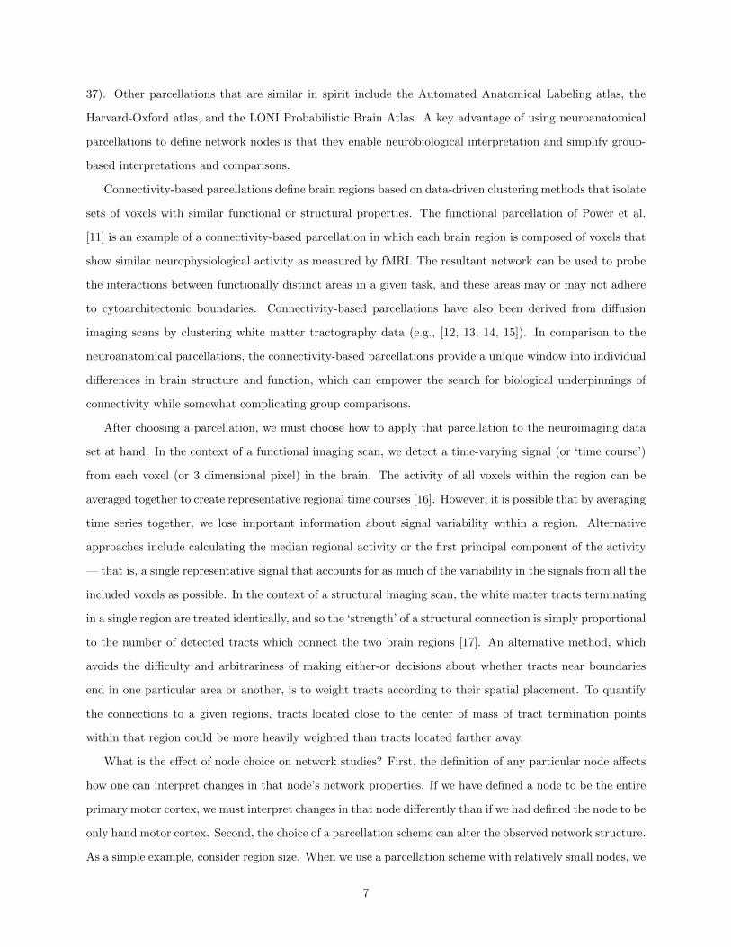
37). Other parcellations that are similar in spirit include the Automated Anatomical Labeling atlas, the
Harvard-Oxford atlas, and the LONI Probabilistic Brain Atlas. A key advantage of using neuroanatomical
parcellations to define network nodes is that they enable neurobiological interpretation and simplify group-
based interpretations and comparisons.
Connectivity-based parcellations define brain regions based on data-driven clustering methods that isolate
sets of voxels with similar functional or structural properties. The functional parcellation of Power et al.
[11] is an example of a connectivity-based parcellation in which each brain region is composed of voxels that
show similar neurophysiological activity as measured by fMRI. The resultant network can be used to probe
the interactions between functionally distinct areas in a given task, and these areas may or may not adhere
to cytoarchitectonic boundaries. Connectivity-based parcellations have also been derived from diffusion
imaging scans by clustering white matter tractography data (e.g., [12, 13, 14, 15]). In comparison to the
neuroanatomical parcellations, the connectivity-based parcellations provide a unique window into individual
differences in brain structure and function, which can empower the search for biological underpinnings of
connectivity while somewhat complicating group comparisons.
After choosing a parcellation, we must choose how to apply that parcellation to the neuroimaging data
set at hand. In the context of a functional imaging scan, we detect a time-varying signal (or ‘time course’)
from each voxel (or 3 dimensional pixel) in the brain. The activity of all voxels within the region can be
averaged together to create representative regional time courses [16]. However, it is possible that by averaging
time series together, we lose important information about signal variability within a region. Alternative
approaches include calculating the median regional activity or the first principal component of the activity
— that is, a single representative signal that accounts for as much of the variability in the signals from all the
included voxels as possible. In the context of a structural imaging scan, the white matter tracts terminating
in a single region are treated identically, and so the ‘strength’ of a structural connection is simply proportional
to the number of detected tracts which connect the two brain regions [17]. An alternative method, which
avoids the difficulty and arbitrariness of making either-or decisions about whether tracts near boundaries
end in one particular area or another, is to weight tracts according to their spatial placement. To quantify
the connections to a given regions, tracts located close to the center of mass of tract termination points
within that region could be more heavily weighted than tracts located farther away.
What is the effect of node choice on network studies? First, the definition of any particular node affects
how one can interpret changes in that node’s network properties. If we have defined a node to be the entire
primary motor cortex, we must interpret changes in that node differently than if we had defined the node to be
only hand motor cortex. Second, the choice of a parcellation scheme can alter the observed network structure.
As a simple example, consider region size. When we use a parcellation scheme with relatively small nodes, we
7
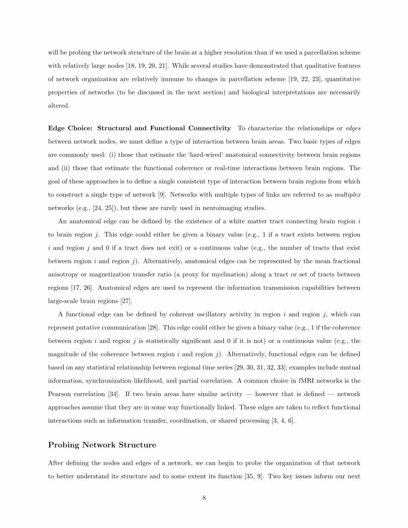
will be probing the network structure of the brain at a higher resolution than if we used a parcellation scheme
with relatively large nodes [18, 19, 20, 21]. While several studies have demonstrated that qualitative features
of network organization are relatively immune to changes in parcellation scheme [19, 22, 23], quantitative
properties of networks (to be discussed in the next section) and biological interpretations are necessarily
altered.
Edge Choice: Structural and Functional Connectivity To characterize the relationships or edges
between network nodes, we must define a type of interaction between brain areas. Two basic types of edges
are commonly used: (i) those that estimate the ‘hard-wired’ anatomical connectivity between brain regions
and (ii) those that estimate the functional coherence or real-time interactions between brain regions. The
goal of these approaches is to define a single consistent type of interaction between brain regions from which
to construct a single type of network [9]. Networks with multiple types of links are referred to as multiplex
networks (e.g., [24, 25]), but these are rarely used in neuroimaging studies.
An anatomical edge can be defined by the existence of a white matter tract connecting brain region i
to brain region j. This edge could either be given a binary value (e.g., 1 if a tract exists between region
i and region j and 0 if a tract does not exit) or a continuous value (e.g., the number of tracts that exist
between region i and region j). Alternatively, anatomical edges can be represented by the mean fractional
anisotropy or magnetization transfer ratio (a proxy for myelination) along a tract or set of tracts between
regions [17, 26]. Anatomical edges are used to represent the information transmission capabilities between
large-scale brain regions [27].
A functional edge can be defined by coherent oscillatory activity in region i and region j, which can
represent putative communication [28]. This edge could either be given a binary value (e.g., 1 if the coherence
between region i and region j is statistically significant and 0 if it is not) or a continuous value (e.g., the
magnitude of the coherence between region i and region j). Alternatively, functional edges can be defined
based on any statistical relationship between regional time series [29, 30, 31, 32, 33]; examples include mutual
information, synchronization likelihood, and partial correlation. A common choice in fMRI networks is the
Pearson correlation [34]. If two brain areas have similar activity — however that is defined — network
approaches assume that they are in some way functionally linked. These edges are taken to reflect functional
interactions such as information transfer, coordination, or shared processing [3, 4, 6].
Probing Network Structure
After defining the nodes and edges of a network, we can begin to probe the organization of that network
to better understand its structure and to some extent its function [35, 9]. Two key issues inform our next
8

steps: statistical noise in the data and the presence of multiple scales of interest in the network. In the
recent literature, several methods have been proposed to address each of these factors and here we briefly
review these approaches.
Statistical Noise. In empirical measurements of brain activity and anatomy, noise affects our confidence
in the estimated strength of edges in both anatomical and functional brain networks. In a functional network,
should we treat two regions as connected if their activity profiles are correlated with a Pearson’s r of 0.01?
Or in an anatomical network, should we treat two regions as being connected if they are linked by a single
streamline as estimated by white matter tractography algorithms? Answers to these questions depend on
our understanding of the noise present in the data. Noise in these data sets can stem from biological,
measurement, or data-processing sources or a complicated combination of all three.
To maximize the power to detect neurophysiologically relevant connectivity patterns, two main solutions
have been proposed. In one approach, we can test the statistical significance of each edge in the network,
then remove statistically non-significant edges from the network by setting their value to 0. We then study
the organization of the remaining (statistically significant) edges. This approach is often utilized in the
context of functional networks. If edges are defined by statistical similarities in regional brain time series,
the significance of the elements of the resulting connectivity matrix are affected by the large number of
tests that have been performed, which significantly increases the chances of Type I (false positive) errors.
Several multiple comparisons correction methods for these errors, such as Bonferroni and False Discovery
Rate [36], have been proffered (e.g., [16, 1]), although some argue that these approaches are too stringent
for network-based analyses [37]. A false positive correction in which edges are retained if their p-values are
less than 1/N where N is the number of nodes in the network may be a suitable compromise (e.g., [38, 39]).
In a second approach, we do not perform any statistical thresholding on the edge weights. Instead, we
study the entire network (inclusive of the noise), and then compare that network structure to null models
that have been constructed to account for one or more sources of noise [2]. For example, we can construct a
null model for functional brain networks by creating surrogate time series that maintain the mean, variance,
and autocorrelation of the original signal. By comparing the real brain network to this null model, we can
identify features of the network that cannot simply be accounted for linear properties of the time series. A
critical area of ongoing research is the development of more sophisticated null models that seek to account
for more complicated structure in biological networks such as growth and development, temporal dynamics,
and physical embedding of the network inside of the skull [40, 41, 2].
9
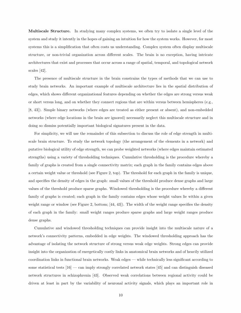
Multiscale Structure. In studying many complex systems, we often try to isolate a single level of the
system and study it intently in the hopes of gaining an intuition for how the system works. However, for most
systems this is a simplification that often costs us understanding. Complex system often display multiscale
structure, or non-trivial organization across different scales. The brain is no exception, having intricate
architectures that exist and processes that occur across a range of spatial, temporal, and topological network
scales [42].
The presence of multiscale structure in the brain constrains the types of methods that we can use to
study brain networks. An important example of multiscale architecture lies in the spatial distribution of
edges, which shows different organizational features depending on whether the edges are strong versus weak
or short versus long, and on whether they connect regions that are within versus between hemispheres (e.g.,
[8, 43]). Simple binary networks (where edges are treated as either present or absent), and non-embedded
networks (where edge locations in the brain are ignored) necessarily neglect this multiscale structure and in
doing so dismiss potentially important biological signatures present in the data.
For simplicity, we will use the remainder of this subsection to discuss the role of edge strength in multi-
scale brain structure. To study the network topology (the arrangement of the elements in a network) and
putative biological utility of edge strength, we can probe weighted networks (where edges maintain estimated
strengths) using a variety of thresholding techniques. Cumulative thresholding is the procedure whereby a
family of graphs is created from a single connectivity matrix; each graph in the family contains edges above
a certain weight value or threshold (see Figure 2, top). The threshold for each graph in the family is unique,
and specifies the density of edges in the graph: small values of the threshold produce dense graphs and large
values of the threshold produce sparse graphs. Windowed thresholding is the procedure whereby a different
family of graphs is created; each graph in the family contains edges whose weight values lie within a given
weight range or window (see Figure 2, bottom; [44, 43]). The width of the weight range specifies the density
of each graph in the family: small weight ranges produce sparse graphs and large weight ranges produce
dense graphs.
Cumulative and windowed thresholding techniques can provide insight into the multiscale nature of a
network’s connectivity patterns, embedded in edge weights. The windowed thresholding approach has the
advantage of isolating the network structure of strong versus weak edge weights. Strong edges can provide
insight into the organization of energetically costly links in anatomical brain networks and of heavily utilized
coordination links in functional brain networks. Weak edges — while technically less significant according to
some statistical tests [16] — can imply strongly correlated network states [45] and can distinguish diseased
network structures in schizophrenia [43]. Observed weak correlations between regional activity could be
driven at least in part by the variability of neuronal activity signals, which plays an important role in
10

Cumulative Thresholding
Windowed Thresholding
Density: 0.1 0.3 0.5 0.7 0.9
Density: 0.2 0.2 0.2 0.2 0.2
10% strongest edges retained
90% strongest edges retained
20% strongest edges retained
20% weakestedges retained
WeightedNetwork
Figure 2: Probing Multiscale Architecture in Network Edge Weights. Multiscale structure in aweighted network (left) can be probed using thresholding techniques. (A) Cumulative thresholding is theprocedure whereby a connectivity matrix is separated into a set of graphs that contain edges above a certainweight value or threshold. (B) Windowed thresholding is the procedure whereby a a connectivity matrixis separated into a set of graphs that contain edges whose weight values lie within a given weight range orwindow [44, 43].
cognitive function [46], development [47], and recovery from injury [48].
Generating Network Diagnostics
A network ‘diagnostic’ is simply a named measurement used to describe a network’s properties. These
properties can then be compared across different networks. For example, a patient’s network diagnostics can
be compared with those of a healthy participant; or a human brain network can be compared to a worm
neuronal network to see whether the properties captured by that diagnostic are shared by neural systems in
different species [20].
Network diagnostics are not quantities like mass, entropy, or replication rate that a priori have a clear
physical meaning. Instead, they are mathematical definitions that formalize architectural concepts specific
to network science [49]. As an outsider, this jargon can at times make the field seem impenetrable. However,
upon closer inspection, many diagnostics captures an intuitive property of interconnected systems that can
often be easily interpreted in the context of the brain [27, 50].
Local, Global, and Mesoscale Properties We can use network diagnostics to study the organization
of anatomical and functional brain networks across spatial scales, from the neighborhood of the network
11

surrounding a single brain area (captured using local statistics) to the architecture of the entire network
(captured using global statistics). A typical local diagnostic is the clustering coefficient C, which relates
to the likelihood that a node’s neighbors are connected to one another, forming triangles or loops (see
Figure 1C1). The clustering coefficient can be calculated for each node separately, and then the values
can be averaged across nodes to determine a mean clustering coefficient for the network. A brain-centric
interpretation of the clustering coefficient is that it might quantify the amount of local information integration
[27, 4].
A typical global diagnostic is the average shortest path length L. The shortest path between node i and
node j is the smallest number of edges that must be traversed to get from node i to node j. The average
shortest path is the mean shortest path over all possible pairs of nodes in the graph (see Figure 1C2). A
brain-centric interpretation of the average shortest path length is that it might quantify the amount of global
information segregation [27, 4]. A related concept — the network efficiency [51, 52] — is also calculated based
on shortest paths through a graph. Networks with high efficiency have short path lengths and networks with
low efficiency have long path lengths. Network efficiency has been interpreted in relation to the efficiency of
information processing in the brain [53, 27].
Mesoscale diagnostics (“meso-” means “middle”) capture intermediate-level properties of network organi-
zation. Rather than focusing on either the local neighborhood of a node or the global structure of the entire
graph, mesoscale diagnostics characterize the organization of groups of nodes. For example, core-periphery
diagnostics enable us to uncover a core of densely and mutually interconnected nodes and a periphery of
sparsely connected nodes (see Figure 1C3, left ; [54, 55]). Core-periphery organization might confer robustness
to the brain’s structural core [56] and enable a balance between stability and adaptivity in brain dynamics
[57]. Modularity is another type of mesoscale property in which sets of nodes form densely connected sub-
groups (see Figure 1C3, right ; [58, 59]). Modular organization provides a natural substrate for the combined
integration and segregation of information processing arguably required for healthy brain function [4].
Despite the changing fashions for particular diagnostics (for example, small-worldness: a buzzword of
the early 2000s which is now falling somewhat out of favor), no single diagnostic can capture all of the
important organizational properties of networks [49]. The library of network diagnostics is continually
growing as applied mathematicians, physicists, computer scientists, and others define new mathematical
entities to capture previously unexplored patterns in network structure. While each diagnostic has a unique
mathematical definition, it is possible for several diagnostics to produce values that are highly correlated
with one another across network samples (e.g., across different brains). A current challenge is to determine
the families of network diagnostics that provide complementary but not necessarily independent information
about functional and anatomical brain organization [38].
12

Interpretational Caveats Network diagnostics can be intuitively interpreted in terms of information pro-
cessing: high clustering can suggest that information is processed in local domains, while short path-length
can suggest that information is being transmitted over longer distances within the network. However, the bi-
ological meaning of these interpretations requires a conceptual leap from topological to biological terms which
are semantically equivalent, but not necessarily conceptually inter-changeable [60]. Biological efficiency, for
example, has evolutionary implications which may not apply to network efficiency. More generally, such
interpretations of network diagnostics require empirical validation demonstrating the relationship between
quantifiable estimates of information processing or biological efficiency and network characteristics. Until
then, a cautious interpretation of network diagnostics need not hamper the utility of these approaches in
prediction, classification, diagnosis, and monitoring and in the study of system level dynamics underlying
cognitive function.
Using Diagnostics to Probe Brain Network Structure We have shown how a variety of different
networks could be produced from a single brain scan. The network diagnostics generated will vary consider-
ably, depending on whether a weighted or binary network is used, whether we take a cumulative or windowed
thresholding approach, and what range of connection densities we choose to consider. For example, we can
see in Figure 3A that the value of the clustering coefficient tends to be small for sparse graphs and large for
dense graphs, where neighbors of a node are more likely to also be connected to one another (see Figure 3A).
The value of network efficiency shows the opposite effect: large values characterize sparse graphs and small
values characterize dense graphs, where any pair of nodes is likely to be connected.
Given this variation, how do we choose which actual numbers should be used to represent a sample,
when it is compared to another? The characteristic curves of diagnostic values as a function of graph
density or mean edge weight provide useful signatures of brain networks in different states (e.g., health
and disease, or various task states). We can collapse a curve extracted from a single participant into one
number by calculating the area under the curve (AUC) [61]. The advantage of this procedure is that we
can then determine group differences in this value by performing a simple t-test or permutation test. The
disadvantage of this procedure is that we have necessarily lost information about the shape of the curve.
Two groups might have identical AUC values but quite different curve shapes. An alternative approach is to
use functional data analysis, a statistical technique developed for the principled study of curves, to determine
whether the area between the curves is significantly different from zero [43, 62] (see Figure 3B).
While network diagnostic values and curves provide insight into the organization of the network, it is the
mapping of these values back to brain regions that enables us to make fine-grained biological interpretations
of our data. Different network diagnostics can display very different spatial distributions across the surface of
13

0 0.2 0.4 0.6 0.8 10
0.5
1
Clus
terin
g Co
e�ci
ent
Density0
1
2
log (Netw
ork E�ciency)
10
A B
0 0.2 0.4 0.6 0.8 10
0.5
1
Clus
terin
g Co
e�ci
ent
Density
Group 1
Group 2
Area
Network E�ciency
Clustering Coe�cientC
57.5
75.2
21.2
9.4
Figure 3: Using Diagnostics to Probe Brain Network Structure. (A) Clustering coefficient (lefty-axis, black) and network efficiency (right y-axis, light gray) as a function of network density as estimatedusing cumulative thresholding techniques. (B) Schematic of mean clustering coefficient versus density curvesfor two sets of participants: Group 1 (thin, light gray dashed line) and Group 2 (thick, dark gray dashedline). Functional data analysis is a statistical framework that can be used to determine whether the areabetween the two curves is significant in comparison to a null model. (C) Area under the clustering coefficientversus density curve (top) and the network efficiency versus density curve (bottom) for 112 regions of thebrain, defined according to the Harvard-Oxford atlas (see [1, 2] for additional details on this data set).
the brain (see Figure 3C). For example, in an early motor skill learning task [1, 2], the clustering coefficient is
strong in the primary motor cortex and weak in visual association areas while the network efficiency displays
the opposite trend. Such maps can be constructed for individual participants or for groups of participants
and enable us to link our results to the large body of neuroimaging literature isolating functions of individual
brain regions.
Experimental Design
Since its inception, network neuroscience has predominantly been exploratory in nature. In network-based
studies of the brain, researchers are constantly fine-tuning methodological approaches and isolating empirical
questions that are amenable to these approaches. Often these studies have included a re-analysis of previously
published data, which had initially been examined from a more traditional perspective. The use of previously
acquired data is unquestionably justified for many reasons, including but not limited to the use of taxpayer
money for research studies, the time spent by subject participants in volunteering for the study, the difficulty
in obtaining patient data, and the richness of data acquired by current neuroimaging techniques that cannot
be mined completely using a single analytic approach. These studies have provided extensive early validation
of network methods and their use in understanding the human brain.
However, the re-analysis of previously acquired data has its disadvantages. The most critical disadvantage
is that these studies were often not conceived with network-based hypotheses in mind. New data acquired
14
using experimental paradigms specifically designed to test network hypotheses will open up entirely new
fields of inquiry. The development of such paradigms and hypotheses is an important frontier in network
neuroscience.
What Can Network Approaches Tell Us?
Is network neuroscience an enlightening new approach to cognitive science or is it simply an interesting
intellectual exercise for the mathematically inclined? The empirical evidence to date strongly supports the
former conclusion.
The first type of evidence comes from the fact that network neuroscience has provided diagnostics that
display close relationships with more traditional measurements or known quantities. For example, people
with a variety of psychiatric and neurological diseases have differently connected brains than people who
are healthy [6]. When people perform different tasks, their brain regions interact differently, leading to
alterations in network diagnostics (e.g., [63]). Over both long and short time scales (from years [64] to days
and minutes [1]), your brain changes in how different regions interact with each other. As your behavior
changes, so do your brain networks [65].
Together, these results provide important validation of the network approach to neuroscience. But not
all of these results are surprising or ground-breaking. The results often grab the attention of the media
instead because they directly address the perennial problem of cartesian dualism that pervades both lay and
medical thinking: linking the mind to the brain. Indeed, studies demonstrating brain correlates of behaviors
or psychiatric disease continually inform, and provoke new developments in, the philosophy of mind. In
addition to their philosophical appeal, network methods can also display these results in a quantitative and
visually appealing way. But do these results fundamentally advance our understanding of how the human
brain works?
Network Neuroscience as Explanation
The growing consensus in the community is a resounding “Yes”. Network science provides a fundamen-
tally new level of explanation for cognitive function. And what do we mean by an “explanation”? Among
other things, an explanation can (i) describe phenomena in terms of more fundamental and general princi-
ples, or (ii) provide a causal history of the phenomena [66]. Reductionist models of biological phenomena
have traditionally provided explanations of the second form (providing causal histories) but in general have
difficulty providing explanations of the first form (linking to fundamental principles). Network science, how-
ever, provides inherently new information about how the brain works in relation to general mathematical
15

and physical principles, and it is this new information that informs novel hypotheses, interpretations, and
empirical studies.
Shifting Conceptual Paradigms Network science has supported a fundamental paradigm shift in the
conceptual framework that we use for neuroscientific inquiry. By placing significant weight on the importance
of interactions, network methods stand in contrast to other approaches focused primarily on the localization
of cognitive functions to specific brain areas through the study of local brain activity. Instead, the princi-
pled investigation of time-dependent communication between brain regions, facilitated by network methods,
has enabled the discovery and description of both intrinsic (the default mode network [67]) and extrinsic
connectivity phenomena.
Revealing Organizational Principles Network science can be used to uncover organizational principles
of complex systems. As an example, consider the use of network science in the identification of evolutionary
and metabolic constraints on brain structure [20, 68]. By studying network architecture present in natural
organisms, from human to worm, we can infer fundamental principles of brain organization, such as cost-
efficiency in network organization [68], and posit their alteration in disease states [69]. Extracting these
guiding principles is of critical importance in building an expanded theoretical neuroscience, and is a necessary
complement to the accrual of increasingly detailed accounts of specific brain areas, pathways, and molecules.
Distilling Mechanisms of Disease In addition to uncovering organizational principles in the healthy
brain, network neuroscience has provided new insights into the mechanisms of disease. In Alzheimer’s dis-
ease, for example, regions of dense functional connectivity (also known as network hubs) correspond to
areas of greatest plaque deposition [70]. In contrast to descriptions of plaque density from non-systems
approaches, these results from network science suggest a disease mechanism: high metabolic function, in-
formation processing, and structural connectivity in brain network hubs might augment the pathological
cascade in Alzheimer’s disease. Network neuroscience methods have also played a primary role in our grow-
ing understanding of schizophrenia as a brain-wide pathology, characterized by extensive dysconnectivity
rather than localized abnormal activity [71]. Even in the context of stroke, network methods have been used
to show that communication pathways are altered far from the lesioned site [72], illustrating the wide-ranging
possible uses of network methods in the study of both localized injury and distributed disease.
16
Network Neuroscience as a Young Field
Despite these exciting recent advances, network neuroscience is still a very young field and many challenges
remain. Particularly salient frontiers evident in the recent literature include the following:
• Network Dynamics. The human brain is a dynamic system [73] underpinning the complexities of
cognitive function. The extension of network methods to characterize the temporal changes in putative
communication patterns in the brain is necessary to understand the constantly evolving nature of
cognition [74, 1, 75, 76].
• Neurophysiological & Genetic Drivers of Network Organization. The brain networks that we observe
are driven by lower level physiological processes (e.g., [43, 77]) and genetic phenomena (e.g., [78,
79]). Determining the role of molecular and cellular dynamics in large-scale network and systems
neuroscience is critical for a mechanistic understanding of brain development and function.
• Network-Based Prediction. Network approaches provide novel possibilities for classification and pre-
diction. Machine learning, mathematical modeling, and statistical analyses have shown promise in
predicting brain state (e.g., [80]), disease progression (e.g., [81]), and potential receptivity to neurore-
habilitation efforts [1, 57].
• Network Approaches to Behavior, Perception, and Evolution. Applications of network methods outside
of neuroimaging could provide important insights into cognitive function. For example, the network
concept of community structure has been used to capture the organization of human movements (e.g.,
[82]), the temporal relationships between concepts (e.g., [83]), and the genetic interactions underlying
cellular machines impacting on neural function (e.g., [84]).
Together, these frontiers promise to provide important progress in our understanding of cognitive function,
its neurophysiological and genetic underpinnings, and its relationship to behavior.
As with any young field, the scientific excitement of network neuroscience is paired with its growing
pains. First, it is not always clear how to translate the findings of network neuroscience to the clinic, be
that in the development of antipsychotic drugs or in the rehabilitation of injured patients. Progress in this
area requires greater progress in clinical systems neuroscience. Second, sources of noise in specific subject
populations (e.g., movement in adolescents or in people with schizophrenia) can produce network signatures,
which if not adequately corrected for, can lead to the inaccurate identification of group differences in network
structure. Indeed, the identification and understanding of individual differences in brain connectivity will be
an important area of growth in the coming years. Third, some network diagnostics and concepts can appear
to be fads: small-worldness and power-law degree distributions were of great interest until it was shown
17

that most real world networks are small-world and power-law degree distributions do not necessarily imply
a specific underlying mechanism (e.g., criticality) [85]. Finally, simple network representations of complex
systems like the brain necessarily abstract away many potentially important biological details: nodes are not
all identical, but instead have different structural and functional properties (e.g., [8]). A critical effort in the
coming years will be to extend network representations to take into account these inter-regional differences to
create more biologically realistic models of this complex data. Despite these growing pains, network science
is a vibrant, rapidly growing field that brings with it exceptional promise for both empirical and theoretical
neuroscience.
Concluding Remarks
In this chapter, we have discussed why network methods provide an interesting approach to the study of
neuroscientific problems in general. The promise, challenges, and controversies of network neuroscience make
it an exciting area, ripe for rapid progress, and crying out for new minds. To encourage you to dive in, we
have provided a list of reviews and resources to explore in Box 1 and a list of helpful toolboxes in Box 2. We
hope that these tools will be of use to you as you walk the paths of methodological innovation and scientific
discovery.
Box 1: Reviews and Resources
• Several reviews address the general techniques used in applying network science to neuroscience data
[86, 87, 4, 88, 3, 89, 90, 91, 68, 92, 93, 92].
• A smaller number of reviews focus on network applications in disease [6, 94, 95, 71].
• “Networks: An Introduction” is an excellent network science textbook [49].
• “Networks of the Brain” is a wonderful book about the application of network science to neuroscience
[27].
18
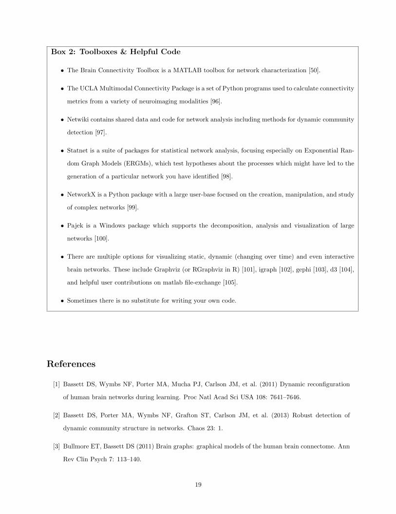
Box 2: Toolboxes & Helpful Code
• The Brain Connectivity Toolbox is a MATLAB toolbox for network characterization [50].
• The UCLA Multimodal Connectivity Package is a set of Python programs used to calculate connectivity
metrics from a variety of neuroimaging modalities [96].
• Netwiki contains shared data and code for network analysis including methods for dynamic community
detection [97].
• Statnet is a suite of packages for statistical network analysis, focusing especially on Exponential Ran-
dom Graph Models (ERGMs), which test hypotheses about the processes which might have led to the
generation of a particular network you have identified [98].
• NetworkX is a Python package with a large user-base focused on the creation, manipulation, and study
of complex networks [99].
• Pajek is a Windows package which supports the decomposition, analysis and visualization of large
networks [100].
• There are multiple options for visualizing static, dynamic (changing over time) and even interactive
brain networks. These include Graphviz (or RGraphviz in R) [101], igraph [102], gephi [103], d3 [104],
and helpful user contributions on matlab file-exchange [105].
• Sometimes there is no substitute for writing your own code.
References
[1] Bassett DS, Wymbs NF, Porter MA, Mucha PJ, Carlson JM, et al. (2011) Dynamic reconfiguration
of human brain networks during learning. Proc Natl Acad Sci USA 108: 7641–7646.
[2] Bassett DS, Porter MA, Wymbs NF, Grafton ST, Carlson JM, et al. (2013) Robust detection of
dynamic community structure in networks. Chaos 23: 1.
[3] Bullmore ET, Bassett DS (2011) Brain graphs: graphical models of the human brain connectome. Ann
Rev Clin Psych 7: 113–140.
19

[4] Bullmore E, Sporns O (2009) Complex brain networks: Graph theoretical analysis of structural and
functional systems. Nat Rev Neurosci 10: 186–198.
[5] Bullmore E, Barnes A, Bassett DS, Fornito A, Kitzbichler M, et al. (2009) Generic aspects of complexity
in brain imaging data and other biological systems. Neuroimage 47: 1125–1134.
[6] Bassett DS, Bullmore ET (2009) Human brain networks in health and disease. Curr Opin Neurol 22:
340–347.
[7] Honey CJ, Sporns O, Cammoun L, Gigandet X, Thiran JP, et al. (2009) Predicting human resting-state
functional connectivity from structural connectivity. Proc Natl Acad Sci USA 106: 2035–40.
[8] Hermundstad AM, Bassett DS, Brown KS, Aminoff EM, Clewett D, et al. (2013) Structural foundations
of resting-state and task-based functional connectivity in the human brain. Proc Natl Acad Sci U S A
110: 6169–6174.
[9] Butts CT (2009) Revisiting the foundations of network analysis. Science 325: 414–416.
[10] Brodmann K (1909) Vergleichende Lokalisationslehre der Grosshirnrinde. Leipzig : Johann Ambrosius
Barth.
[11] Power JD, Cohen AL, Nelson SM, Wig GS, Barnes KA, et al. (2011) Functional network organization
of the human brain. Neuron 72: 665–78.
[12] Cloutman LL, Lambon Ralph MA (2012) Connectivity-based structural and functional parcellation of
the human cortex using diffusion imaging and tractography. Front Neuroanat 6.
[13] Gorbach NS, Schutte C, Melzer C, Goldau M, Sujazow O, et al. (2011) Hierarchical information-based
clustering for connectivity-based cortex parcellation. Front Neuroinform 5.
[14] Roca P, Riviere D, Guevara P, Poupon C, Mangin JF (2009) Tractography-based parcellation of the
cortex using a spatially-informed dimension reduction of the connectivity matrix. Med Image Comput
Comput Assist Interv 12: 935–942.
[15] Perrin M, Cointepas Y, Cachia A, Poupon C, Thirion B, et al. (2008) Connectivity-based parcellation
of the cortical mantle using q-ball diffusion imaging. Int J Biomed Imaging 2008.
[16] Achard S, Salvador R, Whitcher B, Suckling J, Bullmore E (2006) A resilient, low-frequency, small-
world human brain functional network with highly connected association cortical hubs. J Neurosci 26:
63–72.
20
[17] Hagmann P, Cammoun L, Gigandet X, Meuli R, Honey CJ, et al. (2008) Mapping the structural core
of human cerebral cortex. PLoS Biol 6: e159.
[18] Zalesky A, Fornito A, Harding IH, Cocchi L, Yucel M, et al. (2010) Whole-brain anatomical networks:
Does the choice of nodes matter? NeuroImage 50: 970–983.
[19] Bassett DS, Brown JA, Deshpande V, Carlson JM, Grafton ST (2011) Conserved and variable archi-
tecture of human white matter connectivity. NeuroImage 54: 1262–1279.
[20] Bassett DS, Greenfield DL, Meyer-Lindenberg A, Weinberger DR, Moore S, et al. (2010) Efficient
physical embedding of topologically complex information processing networks in brains and computer
circuits. PLoS Comput Biol 6: e1000748.
[21] Meunier D, Lambiotte R, Fornito A, Ersche KD, Bullmore ET (2009) Hierarchical modularity in human
brain functional networks. Front Neuroinformatics 3: 37.
[22] de Reus MA, van den Heuvel MP (2013) The parcellation-based connectome: Limitations and exten-
sions. Neuroimage Epub ahead of print.
[23] Wang J, Wang L, Zang Y, Yang H, Tang H, et al. (2009) Parcellation-dependent small-world brain
functional networks: A resting-state fMRI study. Hum Brain Mapp 30: 1511–1523.
[24] Mucha PJ, Richardson T, Macon K, Porter MA, Onnela JP (2010) Community structure in time-
dependent, multiscale, and multiplex networks. Science 328: 876–878.
[25] Bianconi G (2013) Statistical mechanics of multiplex networks: Entropy and overlap. Phys Rev E 87:
062806.
[26] van den Heuvel MP, Mandl RC, Stam CJ, Kahn RS, Hulshoff Pol HE (2010) Aberrant frontal and
temporal complex network structure in schizophrenia: a graph theoretical analysis. J Neurosci 30:
15915–15926.
[27] Sporns O (2010) Networks of the Brain. MIT Press.
[28] Fries P (2005) A mechanism for cognitive dynamics: Neuronal communication through neuronal co-
herence. Trends Cogn Sci 9: 474–480.
[29] David O, Cosmelli D, Friston KJ (2004) Evaluation of different measures of functional connectivity
using a neural mass model. NeuroImage 21: 659–673.
21

[30] Smith SM, Miller KL, Salimi-Khorshidi G, Webster M, Beckmann CF, et al. (2011) Network modelling
methods for FMRI. Neuroimage 54: 875–91.
[31] Dawson DA, Cha K, Lewis LB, Mendola JD, Shmuel A (2013) Evaluation and calibration of functional
network modeling methods based on known anatomical connections. Neuroimage 67: 331–343.
[32] Gates KM, Molenaar PC (2012) Group search algorithm recovers effective connectivity maps for indi-
viduals in homogeneous and heterogeneous samples. Neuroimage 63: 310–319.
[33] Watanabe T, Hirose S, Wada H, Imai Y, Machida T, et al. (2013) A pairwise maximum entropy model
accurately describes resting-state human brain networks. Nat Commun 4: 1370.
[34] Zalesky A, Fornito A, Bullmore E (2012) On the use of correlation as a measure of network connectivity.
Neuroimage 60: 2096–2106.
[35] Proulx S, Promislow D, Phillips PC (2005) Network thinking in ecology and evolution. Trends in
Ecology and Evolution 20: 345–353.
[36] Benjamini Y, Hochberg Y (1995) Controlling the false discovery rate: a practical and powerful approach
to multiple testing. J R Stat Soc Ser B 57: 289-300.
[37] Fornito A, Zalesky A, Breakspear M (2013) Graph analysis of the human connectome: Promise,
progress, and pitfalls. Neuroimage 80C: 426–444.
[38] Lynall ME, Bassett DS, Kerwin R, McKenna P, Muller U, et al. (2010) Functional connectivity and
brain networks in schizophrenia. J Neurosci 30: 9477–9487.
[39] Bassett DS, Meyer-Lindenberg A, Weinberger DR, Coppola R, Bullmore E (2009) Cognitive fitness of
cost-efficient brain functional networks. Proc Natl Acad Sci USA 106: 11747–11752.
[40] Sporns O (2006) Small-world connectivity, motif composition, and complexity of fractal neuronal con-
nections. Biosystems 85: 55–64.
[41] Klimm F, Bassett DS, Carlson JM, Mucha PJ (2013) Resolving structural variability in network models
and the brain. arXiv 1306.2893.
[42] Siebenhuhner F, Bassett DS (2013) Multiscale Analysis and Nonlinear Dynamics. From Genes to the
Brain, Wiley & Sons, volume In Press, chapter Multiscale Network Organization in the Human Brain.
[43] Bassett DS, Nelson BG, Mueller BA, Camchong J, Lim KO (2012) Altered resting state complexity in
schizophrenia. Neuroimage 59: 2196–2207.
22

[44] Schwarz AJ, McGonigle J (2011) Negative edges and soft thresholding in complex network analysis of
resting state functional connectivity data. Neuroimage 55: 1132–1146.
[45] Schneidman E, Berry MJn, Segev R, Bialek W (2006) Weak pairwise correlations imply strongly
correlated network states in a neural population. Nature 440: 1007–1012.
[46] Misic B, Mills T, Taylor MJ, McIntosh AR (2010) Brain noise is task dependent and region specific. J
Neurophysiol 104: 2667–2676.
[47] McIntosh AR, Kovacevic N, Lippe S, Garrett D, Grady C, et al. (2010) The development of a noisy
brain. Arch Ital Biol 148: 323–337.
[48] Raja Beharelle A, Kovacevic N, McIntosh AR, Levine B (2012) Brain signal variability relates to
stability of behavior after recovery from diffuse brain injury. Neuroimage 60: 1528–1537.
[49] Newman MEJ (2010) Networks: An Introduction. Oxford University Press.
[50] Rubinov M, Sporns O (2009) Complex network measures of brain connectivity: Uses and interpreta-
tions. NeuroImage 52: 1059–1069.
[51] Latora V, Marchiori M (2001) Efficient behavior of small-world networks. Phys Rev Lett 87: 198701.
[52] Latora V, Marchiori M (2003) Economic small-world behavior in weighted networks. Eur Phys J B 32:
249–263.
[53] Achard S, Bullmore E (2007) Efficiency and cost of economical brain functional networks. PLoS
Comput Biol 3: e17.
[54] Borgatti SP, Everett MG (1999) Models of core/periphery structures. Social Networks 21: 375–395.
[55] Rombach MP, Porter MA, Fowler JH, Mucha PJ (2012) Core-periphery structure in networks. arXiv
: 1202.2684.
[56] van den Heuvel MP, Sporns O (2011) Rich-club organization of the human connectome. J Neurosci
31: 15775–15786.
[57] Bassett DS, Wymbs NF, Rombach MP, Porter MA, Mucha PJ, et al. (2013) Core-periphery organisa-
tion of human brain dynamics. PLoS Comp Biol In Press.
[58] Porter MA, Onnela JP, Mucha PJ (2009) Communities in networks. Not Amer Math Soc 56: 1082–
1097, 1164–1166.
23
[59] Fortunato S (2010) Community detection in graphs. Phys Rep 486: 75–174.
[60] Rubinov M, Bassett DS (2011) Emerging evidence of connectomic abnormalities in schizophrenia. J
Neurosci 31: 6263–6265.
[61] Ginestet CE, Nichols TE, Bullmore ET, Simmons A (2011) Brain network analysis: separating cost
from topology using cost-integration. PLoS One 6: e21570.
[62] Siebenhuhner F, Weiss SA, Coppola R, Weinberger DR, Bassett DS (2013) Intra- and inter-frequency
brain network structure in health and schizophrenia. PLoS One In Press.
[63] Bassett DS, Meyer-Lindenberg A, Achard S, Duke T, Bullmore E (2006) Adaptive reconfiguration of
fractal small-world human brain functional networks. Proc Natl Acad Sci USA 103: 19518–19523.
[64] Meunier D, Achard S, Morcom A, Bullmore E (2008) Age-related changes in modular organization of
human brain functional networks. NeuroImage 44: 715–723.
[65] Reijmer AaMaLJaGJ Y D andLeemans (2013) Disruption of the cerebral white matternetworkis related
to slowing of information processing speed in patients with type 2 diabetes. Diabetes Epub ahead of
print.
[66] Woodward J (2011) Scientific explanation. In: Zalta EN, editor, The Stanford Encyclopedia of Phi-
losophy. Winter 2011 edition.
[67] Snyder AZ, Raichle ME (2012) A brief history of the resting state: the Washington University per-
spective. Neuroimage 62: 902–910.
[68] Bullmore E, Sporns O (2012) The economy of brain network organization. Nat Rev Neurosci 13:
336–349.
[69] Vertes PE, Alexander-Bloch AF, Gogtay N, Giedd JN, Rapoport JL, et al. (2012) Simple models of
human brain functional networks. Proc Natl Acad Sci U S A 109: 5868–5873.
[70] Buckner RL, Sepulcre J, Talukdar T, Krienen FM, Liu H, et al. (2009) Cortical hubs revealed by
intrinsic functional connectivity: mapping, assessment of stability, and relation to Alzheimer’s disease.
J Neurosci 29: 1860–1873.
[71] Fornito A, Zalesky A, Pantelis C, Bullmore ET (2012) Schizophrenia, neuroimaging and connectomics.
Neuroimage 62: 2296–2314.
24
[72] Crofts JJ, Higham DJ, Bosnell R, Jbabdi S, Matthews PM, et al. (2011) Network analysis detects
changes in the contralesional hemisphere following stroke. Neuroimage 54: 161–169.
[73] Deco G, Jirsa VK, McIntosh AR (2011) Emerging concepts for the dynamical organization of resting-
state activity in the brain. Nat Rev Neurosci 12: 43–56.
[74] Kramer MA, Eden UT, Lepage KQ, Kolaczyk ED, Bianchi MT, et al. (2011) Emergence of persistent
networks in long-term intracranial eeg recordings. J Neurosci 31: 15757–15767.
[75] Allen EA, Damaraju E, Plis SM, Erhardt EB, Eichele T, et al. (2012) Tracking whole-brain connectivity
dynamics in the resting state. Cereb Cortex Epub ahead of print.
[76] Smith SM, Miller KL, Moeller S, Xu J, Auerbach EJ, et al. (2012) Temporally-independent functional
modes of spontaneous brain activity. Proc Natl Acad Sci U S A 109: 3131–3136.
[77] Vaishnavi SN, Vlassenko AG, Rundle MM, Snyder AZ, Mintun MA, et al. (2010) Regional aerobic
glycolysis in the human brain. Proc Natl Acad Sci U S A 107: 17757–17762.
[78] Fornito A, Zalesky A, Bassett D, Meunier D, Yucel M, et al. (2010) Genetic influences on economical
properties of human functional cortical networks. Submitted .
[79] Esslinger C, Walter H, Kirsch P, Erk S, Schnell K, et al. (2009) Neural mechanisms of a genome-wide
supported psychosis variant. Science 324: 605.
[80] Richiardi J, Eryilmaz H, Schwartz S, Vuilleumier P, Van De Ville D (2011) Decoding brain states from
fMRI connectivity graphs. NeuroImage 56: 616–626.
[81] Raj A, Kuceyeski A, Weiner M (2012) A network diffusion model of disease progression in dementia.
Neuron 73: 1204–1215.
[82] Wymbs NF, Bassett DS, Mucha PJ, Porter MA, Grafton ST (2012) Differential recruitment of the
sensorimotor putamen and frontoparietal cortex during motor chunking in humans. Neuron 74: 936–
946.
[83] Schapiro AC, Rogers TT, Cordova NI, Turk-Browne NB, Botvinick MM (2013) Neural representations
of events arise from temporal community structure. Nat Neurosci 16: 486–492.
[84] Conaco C, Bassett DS, Zhou H, Arcila ML, Degnan SM, et al. (2012) Functionalization of a protosy-
naptic gene expression network. Proc Natl Acad Sci U S A 109: 10612–10618.
[85] Stumpf MPH, Porter MA (2012) Critical truths about power laws. Science 51: 665–666.
25
[86] Bassett DS, Bullmore ET (2006) Small-world brain networks. Neuroscientist 12: 512–523.
[87] Reijneveld JC, Ponten SC, Berendse HW, Stam CJ (2007) The application of graph theoretical analysis
to complex networks in the brain. Clin Neurophysiol 118: 2317–2331.
[88] He Y, Evans A (2010) Graph theoretical modeling of brain connectivity. Curr Opin Neurol 23: 341–
350.
[89] Wig GS, Schlaggar BL, Petersen SE (2011) Concepts and principles in the analysis of brain networks.
Ann N Y Acad Sci 1224: 126–146.
[90] Sporns O (2011) The human connectome: a complex network. Ann N Y Acad Sci 1224: 109–125.
[91] Kaiser M (2011) A tutorial in connectome analysis: topological and spatial features of brain networks.
Neuroimage 57: 892–907.
[92] Sporns O (2012) From simple graphs to the connectome: networks in neuroimaging. Neuroimage 62:
881–886.
[93] Stam CJ, van Straaten EC (2012) The organization of physiological brain networks. Clin Neurophysiol
123: 1067–1087.
[94] He Y, Chen Z, Gong G, Evans A (2009) Neuronal networks in Alzheimer’s disease. Neuroscientist 15:
333–350.
[95] Xie T, He Y (2011) Mapping the Alzheimer’s brain with connectomics. Front Psychiatry 2: 77.
[96] Brown JA (2013). Ucla multimodal connectivity package. URL http://ccn.ucla.edu/wiki/index.
php/UCLA_Multimodal_Connectivity_Package.
[97] Mucha PJ (2013). Netwiki. URL http://netwiki.amath.unc.edu/.
[98] Morris M, Handcock MS, Hunter DR, Butts CT, Goodreau SM, et al. (2013). Statnet. URL http:
//statnet.csde.washington.edu/.
[99] Hagberg AA, Schult DA, Swart PJ (2013). Networkx. URL http://networkx.github.io/index.
html.
[100] Batagelj V, Mrvar A (2013). Pajek. URL http://pajek.imfm.si/doku.php.
[101] Bilgin A, Caldwell D, Ellson J, Gansner E, Hu Y, et al. (2013). Graphviz. URL http://www.graphviz.
org/.
26

[102] Csardi G, Nepusz T (2013). igraph. URL http://igraph.sourceforge.net/.
[103] Bastian M, Heymann S, Jacomy M (2013). Gephi. URL https://gephi.org/.
[104] Bostock M (2013). d3. URL http://d3js.org/.
[105] (2013). Matlab file exchange. URL http://www.mathworks.com/matlabcentral/fileexchange/.
27