Network discovery using Reinforcement Learning

Harshavardhan Kamarthi∗ Priyesh Vijayan*† Bryan Wilder‡ Balaraman Ravindran*†

Milind Tambe§

Abstract

A serious challenge when finding influential actors in real-world social networksis the lack of knowledge about the structure of the underlying network. Currentstate-of-the-art methods rely on hand-crafted sampling algorithms to sample nodesin a carefully constructed order and choose opinion leaders from this discoverednetwork to maximize influence spread in the complete network.In this work, we propose a deep reinforcement learning framework graph neuralnetwork modules for network discovery that automatically learns useful node andgraph representations that encode important structural properties of the network.At training time, the method identifies portions of the network such that the nodesselected from this sampled subgraph can effectively influence nodes in the completenetwork. The learned policy can be directly applied on unseen graphs of similardomain. We experiment with real-world social networks and show that the policieslearned by our RL agent provide a 7-23% improvement over the current state-of-the-art method.

1 Introduction

Real-world applications of influence maximization are often limited by the high cost of collectingnetwork data. In particular, we are motivated in particular by the problem of using influencemaximization for HIV prevention among homeless youth [Yad+18; Wil+18a] where gathering thesocial network of the youth who frequent a given homeless centre requires a week or more of effort.Accordingly, an important direction for algorithm development is to create methods which subsamplethe population by surveying only a small subset of nodes to obtain network information. Each nodethat is surveyed reveals its neighbours, and the goal is to carefully select the nodes to be surveyedto choose an influential set of seed nodes. Wilder et al. [Wil+18b] propose an algorithm motivatedby community structure and prove theoretical guarantees for graphs drawn from the stochasticblock model. Later, [Wil+18a] introduced a more practical algorithm called CHANGE based on thefriendship paradox [Fel91]. It uses a simple yet powerful sampling method: For each of the randomseeds, we query one of its neighbors picked at random.

We take a reinforcement learning approach to solve the network discovery problem and propose agraph-based neural network architecture to learn important graph properties from training dataset viaDeep Q-learning algorithm that in turn helps it to query nodes efficiently for network discovery atdeployment. By leveraging structural information from such datasets, our approach learns policieswhich can be deployed on unseen networks from similar domain.

∗Dept. of Computer Science and Engineering, Indian Institute of Technology Madras†Robert Bosch Centre for Data Science and AI, Indian Institute of Technology Madras‡Center for Artificial Intelligence in Society, University of Southern California§Center for Research on Computation and Society, Harvard University

33rd Conference on Neural Information Processing Systems (NeurIPS 2019), Vancouver, Canada.

2 Problem Description

Let the entire unknown graph be G∗ = (V ∗, E∗). Let X ⊆ V ∗ denote a vertex set and let G[X]denote a sub-graph of G∗ induced by X . Let V (G) be the vertex set of a graph G and E(G) be edgeset of G. Let NG(u) be neighbors of vertex u in a graph G, and E(X,Y ) be all edges such that itconnect a node in X and a node in Y .

Initially, we are given |S| seed nodes and a budget of T queries. When we query a node, wediscover the neighbours of the queried node. Let Gt be the sub-graph discovered after t querieswith vertex set, Vt = V (Gt). Let G0 = (S ∪NG∗(S), E(S,NG∗(S))) with S as the initial seed set.During the t+ 1 query, we choose a node ut from Gt and observe Gt+1 = (Vt ∪NG∗(ut), E(Gt) ∪E(NG∗(ut), {ut})). For any observed graph, we can use a standard influence maximization algorithm(which assumes that the graph is known) as an oracle to determine the best set of nodes to activatebased on the available information. Let A = O(G) be the output of this oracle on graph G, and letIG(A) be the expected number of influenced nodes in G on choosing A as the set of initial activenodes. The task is to find a sequence of queries (u0, u1, . . . , uT−1) such that the discovered graphGT is such that it maximizes the IG∗(O(GT )), i.e, we need to discover a sub-graph GT such that thenodes selected by O in GT maximizes the number of nodes influenced in the entire graph, G∗.

(a) Problem overview

(b) Our Neural Architecture

Figure 1: Problem setup and reinforcement learning model

3 Proposed Method

3.1 Information flow model

First we discuss the mechanics of information diffusion across the network. We assume that informa-tion flow is modelled by independent cascade model [KKT05]. We assign the same parameters to themodel as done in [Wil+18c]. Hence, we fix the diffusion probabilities for all edges as 0.1. We fix thebudget for the number of nodes to be activated at 10. Similar to setting in [Wil+18c], before we startnetwork discovery, we are given 5 random seed nodesR and their neighbourhood is revealed. Wehave T = 5 queries to discover the graph GT using which we find the 10 nodes to activate. Thus, thenumber of queries is equal to the number of random seeds (|R| = T ).

3.2 A Markov Decision Process Formulation

We formulate the sequential decision task of network discovery problem discussed in Section 2 as aMDP as follows.

State: At every time-step t, the current state is the discovered graph Gt.

Actions: Given a sub-graph Gt, we can query any of the nodes in Gt which are not yet queried. Thus,the action space is Vt/{S ∪i≤t ui} if t > 0 or is NG∗(S) if t = 0.

Rewards: The actual reward we get after T steps is the number of nodes influenced in the entiregraph, G∗ using the discovered graph, GT which is IG∗(O(GT )). We denote this reward, whichthe model receives at the end of an episode as Ri. However, the range of these values are highly

2

dependent on size and structure of the influenced network. Therefore, we can’t directly use this signalto train with multiple graphs simultaneously.

Using multiple graphs: When using multiple networks, the reward scheme should reflect theeffectiveness of the policy across different networks of varying size and structure. We solve thisproblem by directly comparing the performance of the policy with the performance of a baseline,the state of the art algorithm CHANGE [Wil+18a] and normalize this difference with respect to thedifference between the performance of CHANGE and a lower-bound on optimal performance on thetraining graph.

Rs =IG∗(O(GT ))− CHANGE(G∗)

OPT (G∗)− CHANGE(G∗)(1)

where CHANGE(G∗) is the average number of influenced nodes when the graph is sampled usingCHANGE [Wil+18a] and OPT is the number of influenced nodes when we select the active nodesgiven the knowledge of entire graph. We also add step-rewards at each step to help alleviate rewardsparsity problem and encourage the agent to learn to find larger graphs. The step-reward Rp,t at timet is given as:

Rp,t =|V (Gt)| − |V (Gt−1)|

|V (G∗)|(2)

3.3 Graph representation

In our RL setup, the state at timestep t is the graph discovered at t. To obtain a rich graph (state)representation, we leverage the recent progress in Network Representation Learning with deeplearning models to get efficient graph representations. Specifically, we use a neural network withpermutation invariant graph convolutional layers and differentiable pooling layers [Yin+18] toobtain graph representations. In this work, we use the formulation in [KW16] for GCN layers.While GCNs refine node features by message passing and aggregating, differential pooling seeksto learn a global representation of the graph by aggregating node features in a hierarchical manner.Differentiable pooling (Diffpool) [Yin+18] learn hierarchical representations of the graph, G in anend-end differentiable manner by iteratively coarsening the graph and learning representations for thecoarsened graph at each stage. Diffpool can be used to map a graph to a single finite dimensionalrepresentation by iteratively coarsening the input graph to a graph with a single node and extractingfeatures for this new one node graph.

3.4 State and action representation

The MDP formulation presents us with challenges atypical of most reinforcement learning problems.A social network is a very structured object that can vary in size and complexity. We use Graphconvolutional layers and differentiable pooling to extract useful vector representations that learn toencode the structural properties of the graph. The actions, which are nodes of the networks yet to bequeried, need to be represented as vectors as well.

We use a Diffpool based neural architecture shown in Figure 1b to obtain graph representation.We used DeepWalk embeddings [PAS14] as node features for input layer. We also utilized theseembeddings for representing nodes as action input in Q-network.

3.5 Model training and deployment

For training, we can use single or multiple graphs. At start of an episode, we sample a graph fromtraining set. At every time-step, we choose the node to query by feeding the graph representation ofdiscovered graphGt and node representations of unqueried nodes to select the node vt with maximumpredicted Q-value. On recieving the reward we store the experience in replay buffer and use it forgradient update of all weights in network including GCN and Diffpool layers. The deploymentalgorithm is similar to training algorithm except we freeze the weights of trained Q-network. Thepseudocode of training algorithm is given in supplementary material.

3

3.6 Datasets

We evaluate the effectiveness of our proposed model on datasets from four different domains: 1)Rural Networks, 2) Retweet Networks, 3) Animal Interaction Networks, 4) Homeless Networks Foreach of the 3 families of networks, we divide them into train and test data as shown in Table 1a.

4 Results

The performance metric we used is improve percent. It is the percentage reduction with respect to thegap between OPT and CHANGE (our baseline). (This is same as the scaled reward for last step ofepisode (Equation 1)). The policies learned through reinforcement learning by our agent results in asignificant increase in the number of nodes influenced as shown in Table 1b.

Network category Train networks Test NetworksRural rural1,rural2 rural3,rural4Animal animals1,animals2 animals3, animals4

Retweet copen, occupy assad, isreal,obama,damascus

Homeless a1,spy,mfp b1,cg1,node4,mfp2,mfp3,spy2,spy3

(a) Train and test split for different sets of networks

Network Family improve %Rural 23.76Animal 26.6Retweet 19.7Homeless 7.91

(b) Summary of best results(Scores are averaged test net-works for each class)

Table 1: Experiment tables

Next, we discuss multiple ways we can improve robustness of training in the face of uncertaintiessuch as choosing the right training graph or overcoming lack of actual real-world network to train on.

We found that training with multiple networks gives better performance gains compared to averageperformance gains received by training on single networks. We also used synthetic graphs generatedfrom extracting properties of training graphs(refer to supplementary for more details). Syntheticgraphs can be useful substitutes when we don’t have access to real-world social networks. They canbe used for data-augmentation as well. We saw that the improve percent scores for models using onlysynthetic graphs are better than the average of the scores of models trained from individual networks.For Homeless, Retweet and Rural networks, data augmentation improved the performance over themodel trained on only training graphs. The results are summarized in plots from Figure 2.

Figure 2: improve percent using different combinations of training datasets.(Avg. Individual: Averagescore from policies learned from one of the training graphs. Syn only: Only synthetic graphs fortraining. Real+Syn: Use both synthetic and actual train graphs)

Features of policies learnt Firstly, we observed that the DQN policies almost always discoverlarger graphs than CHANGE does. The DQN policy tends to pick nodes of higher degree centralityand betweenness centrality with respect to the full graph compared to CHANGE, especially duringlater stages of the episode (during steps 4 and 5).

5 Conclusion

We introduce a novel deep Q-learning based method to leverage structural properties of the availablesocial networks to learn effective policies for the network discovery problem for influence maxi-mization on undiscovered social networks. An interesting direction for future work is to exploreapplications of our method to other network discovery problems to by altering the reward function.

4

References

[Ban+13] Abhijit Banerjee et al. “The diffusion of microfinance”. In: Science 341.6144 (2013),p. 1236498.

[Blo+08] Vincent D Blondel et al. “Fast unfolding of communities in large networks”. In: Journalof statistical mechanics: theory and experiment 2008.10 (2008), P10008.

[Dav+15] Stephen Davis et al. “Spatial analyses of wildlife contact networks”. In: Journal of theRoyal Society Interface 12.102 (2015), p. 20141004.

[Fel91] Scott L Feld. “Why your friends have more friends than you do”. In: American Journalof Sociology 96.6 (1991), pp. 1464–1477.

[Han01] Robert A. Hanneman. “Introduction to Social Network Methods”. In: 2001. Chap. 10.[HLL83] Paul W Holland, Kathryn Blackmond Laskey, and Samuel Leinhardt. “Stochastic block-

models: First steps”. In: Social networks 5.2 (1983), pp. 109–137.[KKT03] David Kempe, Jon Kleinberg, and Éva Tardos. “Maximizing the spread of influence

through a social network”. In: KDD. 2003, pp. 137–146.[KKT05] David Kempe, Jon Kleinberg, and Éva Tardos. “Influential nodes in a diffusion model

for social networks”. In: International Colloquium on Automata, Languages, and Pro-gramming. Springer. 2005, pp. 1127–1138.

[KW16] Thomas N Kipf and Max Welling. “Semi-supervised classification with graph convolu-tional networks”. In: arXiv preprint arXiv:1609.02907 (2016).

[Les+09] Jure Leskovec et al. “Community structure in large networks: Natural cluster sizesand the absence of large well-defined clusters”. In: Internet Mathematics 6.1 (2009),pp. 29–123.

[PAS14] Bryan Perozzi, Rami Al-Rfou, and Steven Skiena. “Deepwalk: Online learning of socialrepresentations”. In: Proceedings of the 20th ACM SIGKDD international conferenceon Knowledge discovery and data mining. ACM. 2014, pp. 701–710.

[RA15] Ryan A. Rossi and Nesreen K. Ahmed. “The Network Data Repository with Interac-tive Graph Analytics and Visualization”. In: Proceedings of the Twenty-Ninth AAAIConference on Artificial Intelligence. 2015. URL: http://networkrepository.com.

[Wil+18a] Bryan Wilder et al. “End-to-end influence maximization in the field”. In: Proceedings ofthe 17th International Conference on Autonomous Agents and MultiAgent Systems. Inter-national Foundation for Autonomous Agents and Multiagent Systems. 2018, pp. 1414–1422.

[Wil+18b] Bryan Wilder et al. “Maximizing influence in an unknown social network”. In: Thirty-Second AAAI Conference on Artificial Intelligence. 2018.

[Wil+18c] Bryan Wilder et al. “Maximizing influence in an unknown social network”. In: AAAI.2018, pp. 4743–4750.

[Yad+18] Amulya Yadav et al. “Bridging the Gap Between Theory and Practice in InfluenceMaximization: Raising Awareness about HIV among Homeless Youth.” In: IJCAI. 2018,pp. 5399–5403.

[Yin+18] Zhitao Ying et al. “Hierarchical graph representation learning with differentiable pool-ing”. In: Advances in Neural Information Processing Systems. 2018, pp. 4800–4810.

5

Supplementary Material

A Influence Model

To model information diffusion over the network, we use the standard independent cascade model(ICM) [KKT03], which is the most commonly used model in the literature. In the ICM, every node iseither active or inactive. At the start of the process, every node is inactive except for the seed nodes,S. The process unfolds over a series of discrete time steps. At every step, each newly activated nodeattempts to activate each of its inactive neighbors. Each edge (u, v) is endowed with a propagationprobability pu,v , which gives the probability that u succeeds in influencing v. The process ends whenthere are no newly activated nodes. Our objective is to choose a limited budget of |S| seed nodessuch that the expected number of active nodes at the end of the process is maximized.

B Network Datasets

Here, we describe in detail, the datsets used in our work.

Rural Networks We used the networks gathered by [Ban+13] to the study diffusion of micro-finance in Indian rural households. Different household networks correspond to different rural regions.Each of these networks models a household in a particular region as a node and connects them by anedge if they were related by a set of possible relations such as health, finance, family, friendship, etc.For our experimental study, we considered four such networks (rural1-4).

Retweet Networks These are information flow networks extracted from the Twitter social network.In these networks, each node is a Twitter user, and two users are connected in a graph if one of theusers retweets the tweets of the other. We considered four such retweet networks from the onlinenetwork dataset repository [RA15] 5 viz: occupy, copen, israel, damascus. Each of these retweetnetworks is related to a specific hashtag based information flow. occupy network is related to hashtagsconcerning the famous "Occupy Wall Street" movement, copen is related to mentions about UNconference held in Copenhagen. israel and damascus are concerned about tweets with politicalhashtags that are related to the country Israel and the city of Damascus.

Animal Interaction Networks These networks are a part of the wildlife contact networks collectedby [Dav+15] at different sessions. They specifically studied the physical interactions between Volesand created a contact network. In these contact networks, the animals (Voles) are modeled as nodes,and there is an edge between them if the animals were caught together in one of the traps laid out inthe study. We use four of these contact networks for our experiments (voles1-4).

Homeless Networks We collected homeless networks from various HIV intervention campaignsorganized for homeless youth in Los Angeles. These networks are gathered from previous interventioncampaigns [Wil+18a; Wil+18b]. We considered ten of these networks for our experiments: a1, b1,cg1, node4, mfp2, mfp3, spy2, spy3.

5http://networkrepository.com/

6

Graph Nodes Edges Average degree Averagebetweenness

Louvianmodularity

damascus 3052 3869 2.53 0.00135 0.784israel 3698 4165 2.25 0.0016 0.87rural3 203 410 4.04 0.0165 0.677rural4 204 672 6.59 0.014 0.496voles3 1686 4623 5.48 0.003 0.786voles4 1218 3592 5.89 0.048 0.773mfp2 182 263 2.89 0.018 0.765mfp3 233 368 3.16 0.01 0.748spy2 117 234 4 0.024 0.677spy3 118 237 4.017 0.187 0.685b1 188 375 3.98 0.015 0.626node4 95 123 2.58 0.02 0.768

Table 2: Some properties of networks

7

C Training Algorithm

Algorithm 1: Train NetworkInput :Train Graphs G = {G1, G2, . . . , GK}, number of episodes N , Query budget T , number of

random seeds |S|1 Initialize DQN Qθ and target DQN Qθ′ ;2 Initialize Prioritized Replay Buffer B;3 for episode = 1 to N do4 Choose a graph G from G;5 Select random nodes from G as S;6 V0 = S ∪NG(S);7 Initial graph is G0 = G[V0];8 Compute Deepwalk node embeddings for G0 as φ;9 Get feature matrix F0, adjacency matrix A0 for G0 as S0 = (F0, A0);

10 X ← N(S);11 for t = 0 to T − 1 do12 With probability ε select a random node vt from X else select node

vt ← argmaxv∈X

Qθ(St, φ(v));

13 Query node vt and observe new graph Gt+1;14 Set R← Rp,t (Eqn. 2).;15 If t = T − 1, R← IG∗(O(GT )) +Rp,t;16 Compute scaled influence reward Rt (Eqn. 1);17 Compute Deepwalk node embeddings for Gt+1 as φ;18 Get feature matrix Ft, adjacency matrix At+1 for Gt+1 as St+1 = (Ft+1, At+1);19 X ← nodes not yet queried in Gt+1;20 Add (St, φ(vt), Rt, St+1) to replay buffer D;21 Sample from B and update Qθ;22 end23 Update target network Qθ′ with parameters of Qθ from time to time;24 end

8

D Deployment algorithm

Algorithm 2: Deploy NetworkInput :Trained network Qθ, Graph to be deployed on G, initial random seeds S, query budget T

1 V0 = S ∪NG(S);2 Get the initial graph G[V0];3 Compute Deepwalk node embeddings for G0 as φ;4 Get feature matrix F0, adjacency matrix A0 for G0 as S0 = (F0, A0);5 X ← N(S);6 for t = 0 to T − 1 do7 Select note vt ← argmax

v∈XQθ(St, φ(v));

8 Query node vt and observe new graph Gt+1;9 Compute Deepwalk node embeddings for Gt+1 as φ;

10 Get feature matrix Ft, adjacency matrix At+1 for Gt+1 as St+1 = (Ft+1, At+1);11 X ← nodes not yet queried in Gt+1;12 end13 A ← O(GT );14 Activate nodes in A to start the influence process;

E Other sampling methods

We describe below other sampling methods previously used for network discovery problem.

1. RANDOM-GREEDY: Along with the given initial |S| seeds we query another T nodes atrandom. Then from the subgraph made up of queried nodes, initial seed nodes and theirneighbors we use O to obtain A, nodes to be activated.

2. RECOMMEND: We query a node at random and its neighbors and then add the neighborwith the maximum degree to A. We do this until we exhaust the total budget of 2T queries.If we don’t have sufficient nodes in A then we get the other nodes from O from discoveredsubgraph.

3. SNOWBALL: We start by querying a node at random and its neighbors and then adding theneighbor with the maximum degree to A. Then we again query neighbours of the nodenewly added to A and add the neighbor with the maximum degree to A. In case we havealready queried all neighbors, we again start with querying another random node. Similar toRECOMMEND, we do this till we exhaust out query budget. Then we choose the rest of thenodes from the greedy algorithm O on the discovered graph.

4. CHANGE [Wil+18a]: This is a recent method that was used for effective HIV interventioncampaign. It uses a simple yet powerful sampling method: For each of the random seeds, wequery one of its neighbors picked at random. The model is inspired by friendship paradoxwhich states that the expected degree of a random node’s neighbor is larger than the expecteddegree of a random node. Again we use O to get nodes for A.

The performance of above methods are shown in Table 3.

F Synthetic Graph Generation

We discuss a simple graph generation technique based on the assumption that our social networkshave similar structures to graphs generated by stochastic block models. Real-world social networkshave densely connected components called communities [Les+09]. The nodes of the same communityare tightly connected and nodes of different communities are less frequently connected by anedge. Stochastic Block Models(SBMs), which originated in sociology ([HLL83]), can generategraphs that emulate such structural properties. The nodes of a graph are divided into communities{C1, C2, . . . , Ck}. We add an edge between two nodes of the same community with probability pinand we add an edge between two nodes of different community with probability pout.

9

Graph OPT CHANGE RANDOM-GREEDY Snowball Recommenddamascus 195.4 95.24 98.45 55.85 51.24israel 115.2 30.6 30.9 21.0 22.63rural3 25.2 17.4 17.1 14.48 15.11rural4 45.4 31.5 30.9 14.68 15.25voles3 110.6 33.7 32.38 31.64 33.89voles4 115.7 58.9 56.5 41.72 45.93mfp2 20.56 14.6 14.8 12.69 13.14mfp3 23.45 16.5 16.6 14.97 15.31spy2 21.26 16.01 15.27 14.15 15.13spy3 21.71 16.09 15.88 14.97 15.60b1 24.7 19.1 17.4 15.66 16.11node4 15.84 12.85 13.2 11.40 11.59cg1 17.02 14.17 13.9 11.86 12.16

Table 3: Influence Scores using different state-of-art sampling methods

Given a training graph, we now wish to estimate community sizes {C1, C2, . . . , Ck} and edgeprobabilities pin, pout to generate a graph with similar community based properties. First, we use theLouvain community detection algorithm ([Blo+08]) to partition the graph into communities. We findthe maximum likelihood estimate for pin and pout based on the number of edges that connect nodesof same community and number of edges that connect nodes of different communities in the traininggraph. Then, we construct SBM using the calculated parameters to generate synthetic graphs.

However, Retweet networks don’t usually resemble the stochastic block model structure. Rather, ineach of the communities detected by Louvain Algorithm, we observe that all nodes in the communityare connected to one or two nodes only (see Figure 3). Hence, to generate synthetic graphs similarto retweet networks we tweak the SBM generation procedure. For nodes in each community, wechoose a single node in the community and connect all other nodes to that node. We call this graphgeneration model as Stochastic Star Model(SSM).

(a) copen(b) Generated by SSM

(c) Generated bySBM(Most nodes areisolated)

Figure 3: Difference in graphs generated by SBM and SSM for retweet networks.

We need to be careful to choose models that closely resemble properties of test networks. Table 4shows the large difference in performance when using SBM and SSM models for training on retweetnetworks.

Train graphs damascus israelCHANGE 95.24 30.6copen+occupy 110.8 43.6SSM graphs 116.7 37.4Real + SSM graphs 119.3 42.3SBM Graphs 98.4 32.7Real + SBM Graphs 104.2 41.9

Table 4: Comaprison of influence score for synthetic graphs generated by SBMs and SSMs on retweetnetworks.

10

G Insights on policy learnt: details

G.1 Size of discovered graphs

Tables 5 and 6 provide results on the size of discovered graph (number of vertices and edges) at endof an episode.

Train\Test rural3 rural4 Train\Test voles3 voles4 damascus israelCHANGE 34.0, 40.2 51.3, 63.1 CHANGE 48.4,52.2 71.2,82.4 CHANGE 355.9,351 149.3,145.1rural1 39.8,42 64.5,77.6 voles1 3.5,82.7 80.7,97.0 copen 372.0,370.2 153.8,149.1rural4 2.7,44.5 65.3,76.7 voles2 52.4,82.8 2.8,113.2 occupy 373.6,372.65 159.8,155.0rural1+rural2 38.2,40.5 68.6,84.1 voles1+voles2 70.7,76.1 83.6,95.5 copen+occupy 389.9,384.6 181.1,168.8Syn only 38.4,49.3 67.5,79.8 Syn only 72.2,74.1 88.5,104.2 Syn only 410.7, 409.5 173.5,168.7Real + Syn 38.9,40.4 75.1,85.5 Real + Syn 71.4,77.4 90.0,109.1 Real + Syn 420.5,425.5 12.5,209.7

Table 5: Size of discovered graph. (No. of vertices, No. of edges). Entries with maximum influencescores are bold and entries with largest no. of vertices are underlined)

Train\Test b1 cg1 node4 mfp2 mfp3 spy2 spy3CHANGE 39.28,40.4 26.45,26,6 23.84,23.7 28.3,28.1 33.1,33.2 32.8,40.6 34.7,42.1a1 38.7,40.3 30.23,28.9 28.5,28.1 34.9,35.0 36.3,36.8 37.1,45.3 40.3,51.8spy 43.7,44.5 31.0,30.5 29.1,27.6 36.2,36.8 34.8,35.6 36.8,46.6 36.8,46.2mfp 41.2,44.2 31.5,29.5 28.9,28.2 33.9,34.2 37.5,38.8 39.1,46.7 36.7,45.6Train 43.1,42.7 30.2,39.4 26.2,25.8 33.8,32.7 9.6,40.1 38.2,41.0 37.2,43.7Train+Synth 44.5,47,3 29.5,33.1 27.2,27.8 36.2,38.9 36.1,38.2 9.5,44.2 38.1,42.9Synth 40.9,42.5 4.8,34.5 9.8,30.3 8.6,37.5 35.1,35.3 39.2,46.4 35.9,40.8

Table 6: Size of discovered graph. (No. of vertices, No. of edges). Entries with maximum influencescores are bold and entries with largest no. of vertices are underlined)

G.2 Observations on nodes selected

We observed two recurring events, labelled O1 and O2, during deployment on test networks:O1: The next node to be selected from current sub-graph has minimum degree in the sub-graph.O2: The next node selected in time step t is from set of nodes discovered only in previous step t− 1.

We found that almost all the time, if O2 occurs, O1 also does. We summarize the frequency of bothobservations in Table 7.

Graph O1 O2rural3 0.88 0.5rural4 0.76 0.31voles3 0.66 0.32voles4 0.85 0.31damascus 0.86 0.44israel 0.87 0.28b1 0.93 0.44spy2 0.83 0.58

Table 7: Fraction of queries conforming to observations O1 and O2

Heuristics based on observations To verify that the behaviours O1 and O2 were beneficial forour task, we devised two heuristics.H1: At each step query only from the nodes with minimum degree in current sub-graphH2: At each step query only from the nodes with minimum degree from the set of node discovered inthe previous step. If no new nodes are discovered in the previous step, choose any node not queriedin the discovered graph.

We break all ties by choosing uniformly at random. The performance of the heuristics is summarizedin Table 8.

11

Figure 4: A toy example demonstrating observations O1 and O2

Graph CHANGE H1 H2 Best-DQNrural3 17.4 17.36 17.3 18.75rural4 32.4 32.39 32.6 35.7voles3 33.7 38.7 39.6 45.8voles4 58.9 61.9 72.8 80.2damascus 95.2 93.7 104.9 119.3israel 30.6 30.37 34.2 43.6b1 19.1 19.0 19.4 20.2spy2 16.01 15.877 16.4 17.4

Table 8: Comparisons of scores of heuristics with baselines and best of DQN models for each graph

We observe that H2 outperforms CHANGE for Animals, Homeless and Retweet networks whereasH1 performs similar to CHANGE in all networks. However, the DQN models still perform muchbetter than heuristics. This indicates that the model learns more complex patterns than the simpleheuristics we designed.

G.3 Properties of nodes selected by the policy

To further investigate why the heuristics and our DQN policy performs better, we look at degreecentrality and betweenness centrality of the nodes queried in the true underlying graph, (includingthe nodes and edges not discovered yet).

We call that betweenness and degree centrality of a node computed on the true graph as its truebetweenness centrality and true degree centrality respectively.

In particular, we study three networks: b1 and israel. We compare the true degree centrality and truebetweenness centrality of queried nodes using CHANGE, DQN model and the heuristics discussedabove.

As we can see from Figure 5, the DQN model can recognize nodes with high full degree centralityand full betweenness centrality. For graphs b1 and israel, H2 also picks nodes with higher fullbetweenness centrality than CHANGE but we don’t see much difference in degree of nodes pickedwith respect that picked by CHANGE.

For b1 and israel we further investigate how full degree and betweenness centrality vary acrosstimesteps for H1, H2 and Best DQN model (see Figure 6).

We observe that on average, DQN model finds nodes of high full betweenness centrality and degreecentrality, especially in the last query. Picking nodes with high true degree centrality allows accessto a larger number of nodes during discovery. Betweenness centrality is an important measure ofcentrality of nodes in transportation systems, biological networks and social networks ([Han01]).For network discovery, nodes of high true betweenness centrality could act as a bridge betweendifferent strongly connected communities of nodes for further exploration. In relation to influencemaximization, nodes with true high betweenness centrality can allow the flow of information betweenparts of the network which would otherwise be hard to access.

12

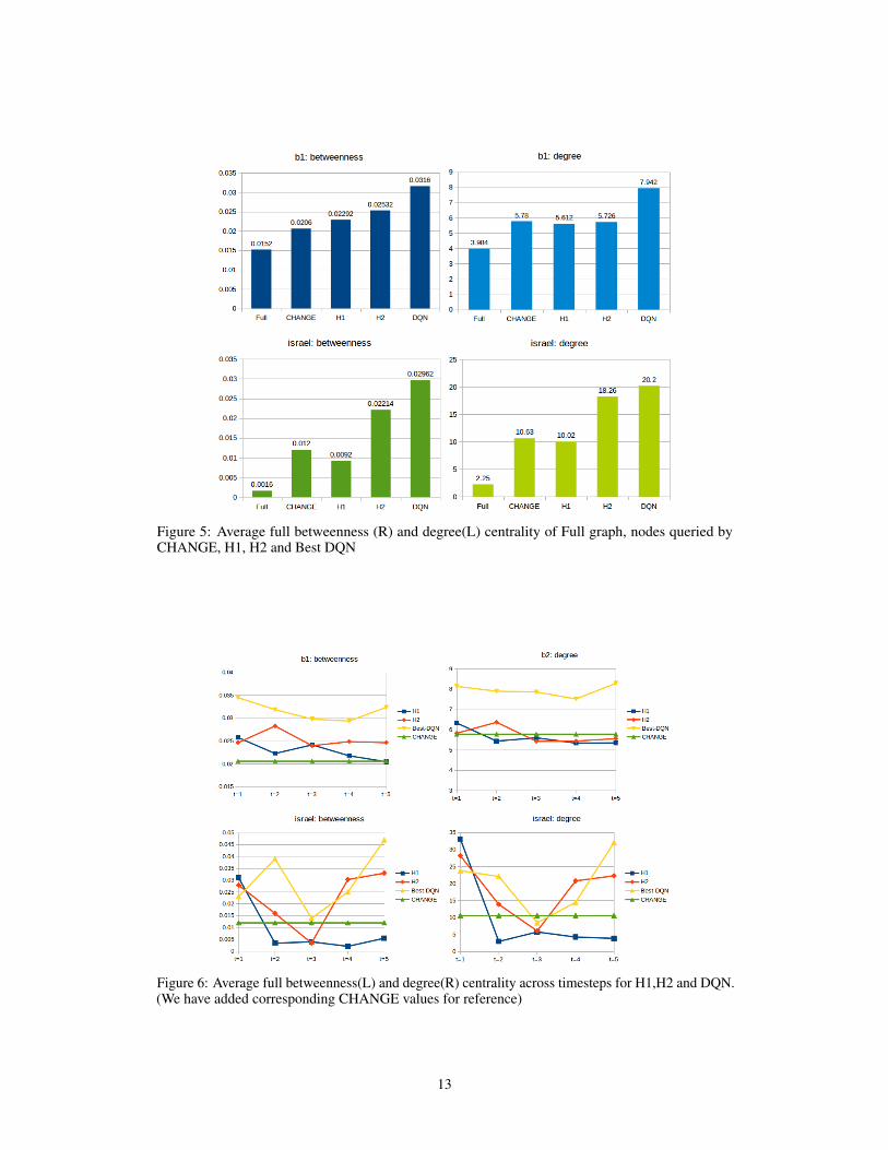
Figure 5: Average full betweenness (R) and degree(L) centrality of Full graph, nodes queried byCHANGE, H1, H2 and Best DQN

Figure 6: Average full betweenness(L) and degree(R) centrality across timesteps for H1,H2 and DQN.(We have added corresponding CHANGE values for reference)

13

H Influence scores for all experiments

Tables 9 and 10 show the influence scores for all experiments performed.

Train\Test rural3 rural4 voles3 voles4 damascus israelCHANGE 17.4 31.5 CHANGE 33.7 58.9 CHANGE 95.24 30.6rural1 18.95 33.1 voles1 42.2 75.3 copen 107.48 36.3rural4 18.1∗ 35.2 voles2 45.3 75.5 occupy 106.2 38.7rural1+rural2 18.2 34.1 voles1+voles2 45.11 78.9 copen+occupy 110.8 43.6Syn only 18.72 34.2 Syn only 45.2 77.3 Syn only 116.7 37.4Real + Syn 18.49 35.7 Real + Syn 45.8 80.2 Real + Syn 119.3 42.3

Table 9: influence scores of all experiments on Rural, Animal and Retweet networks(starred∗ valueswere not statistically significant using t-test with p < 0.01)

Train\Test b1 cg1 node4 mfp2 mfp3 spy2 spy3CHANGE 19.1 14.17 12.85 14.6 16.5 16.01 16.09a1 19.6 14.62 13.63 15.2 17.1 17 18.2spy 19.2∗ 14.53 13.67 15.3 16.5∗ 18 17.6mfp 19.3∗ 14.43 13.56 15.4 17.4 19 17.8Train 19.9 14.8 13.9 15.37 17.76 20 18.1Train+Synth 20.2 14.98 13.83 15.95 17.7 21 18Synth 19.4∗ 14.77 13.7 15.6 17.52 22 17.7

Table 10: influence scores of all experiments on Homeless Networks (starred∗ values were notstatistically significant using t-test with p < 0.01)

14