AUTOMATED DISCOVERY OF OPTIONS IN

REINFORCEMENT LEARNING

A Thesis Presented

by

MARTIN STOLLE

Submitted to the Graduate SchoolMcGill University in partial fulfillmentof the requirements for the degree of

MASTER OF SCIENCE

February 2004

School of Computer Science

c© Copyright by Martin Stolle 2003

All Rights Reserved

ACKNOWLEDGMENTS

I would like to thank my supervisor, Professor Doina Precup, for her guidance and

support of my work starting even at the undergraduate level. Whenever possible, she

was available for consultation and ready to help through her insights into the problems

at hand. Her comments on this thesis were invaluable and resulted in a much clearer

presentation of the ideas. Furthermore, I would like to thank Amy McGovern for her

comments on earlier work and her generous offer to let me use her code for parts of

the experiments. I would also like to thank Bohdana Ratitch for hints and tips during

the coding of the learning algorithms and Francis Perron for his help on the French

resume.

Finally, I would like to give a special thanks to my parents for their love and

support which only made this work and my studies abroad possible. Vielen lieben

Dank!

iii

ABSTRACT

AI planning benefits greatly from the use of temporally-extended or macro-

actions. Macro-actions allow for faster and more efficient planning as well as the

reuse of knowledge from previous solutions. In recent years, a significant amount

of research has been devoted to incorporating macro-actions in learned controllers,

particularly in the context of Reinforcement Learning. One general approach is the

use of options (temporally-extended actions) in Reinforcement Learning [22]. While

the properties of options are well understood, it is not clear how to find new op-

tions automatically. In this thesis we propose two new algorithms for discovering

options and compare them to one algorithm from the literature. We also contribute

a new algorithm for learning with options which improves on the performance of two

widely used learning algorithms. Extensive experiments are used to demonstrate the

effectiveness of the proposed algorithms.

iv

RESUME

La planification de l’IA beneficie considerablement de l’utilisation des actions

temporel-prolonge ou des macro-actions. Les macro-actions tient compte d’une plan-

ification plus rapide et plus efficace aussi bien que la reutilisation de la connaissance de

la solution precedente. Ces dernieres annees, une quantite significative de recherche

a ete consacree a l’incorporation des macro-actions dans la controle appris, en parti-

culier dans le contexte de l’apprentissage par renforcement. Une approche generale

est l’utilisation des options (actions temporel-prolongees) dans l’apprentissage par

renforcement. Tandis que les proprietes des options sont bien connu, il n’est pas

clair comment trouver des nouvelles options automatiquement. Dans cette these

nous proposons deux nouveaux algorithmes pour decouvrir des nouvelles options et

les comparons a un algorithme precedent. Nous contribuons egalement un nouvel

algorithme pour apprendre avec des options qui est plus performante que deux algo-

rithmes d’etude largement repandus. Des experiences etendues sont employees afin

de demontrer l’efficacite de ces algorithmes proposes.

v

TABLE OF CONTENTS

Page

ACKNOWLEDGMENTS . . . . . . . . . . . . . . . . . . . . . . . . . . . iii

ABSTRACT . . . . . . . . . . . . . . . . . . . . . . . . . . . . . . . . . . . iv

RESUME . . . . . . . . . . . . . . . . . . . . . . . . . . . . . . . . . . . . . v

LIST OF TABLES . . . . . . . . . . . . . . . . . . . . . . . . . . . . . . . . viii

LIST OF FIGURES . . . . . . . . . . . . . . . . . . . . . . . . . . . . . . . ix

CHAPTER

1. INTRODUCTION . . . . . . . . . . . . . . . . . . . . . . . . . . . . . . 1

2. BACKGROUND . . . . . . . . . . . . . . . . . . . . . . . . . . . . . . . 4

2.1 Reinforcement Learning . . . . . . . . . . . . . . . . . . . . . . . . . 42.2 Q-Learning . . . . . . . . . . . . . . . . . . . . . . . . . . . . . . . . 62.3 Temporally Extended Actions . . . . . . . . . . . . . . . . . . . . . . 7

2.3.1 Strips . . . . . . . . . . . . . . . . . . . . . . . . . . . . . . . 82.3.2 MacLearn . . . . . . . . . . . . . . . . . . . . . . . . . . . . . 92.3.3 Skills . . . . . . . . . . . . . . . . . . . . . . . . . . . . . . . . 102.3.4 HQ-Learning . . . . . . . . . . . . . . . . . . . . . . . . . . . 122.3.5 Nested Q-Learning . . . . . . . . . . . . . . . . . . . . . . . . 132.3.6 HAM . . . . . . . . . . . . . . . . . . . . . . . . . . . . . . . . 142.3.7 MAXQ . . . . . . . . . . . . . . . . . . . . . . . . . . . . . . . 162.3.8 Drummond’s macro-actions . . . . . . . . . . . . . . . . . . . 17

3. OPTIONS . . . . . . . . . . . . . . . . . . . . . . . . . . . . . . . . . . . 18

3.1 Learning with Options . . . . . . . . . . . . . . . . . . . . . . . . . . 18

3.1.1 SMDP Q-Learning . . . . . . . . . . . . . . . . . . . . . . . . 193.1.2 Intra Option Q-Learning . . . . . . . . . . . . . . . . . . . . . 20

vi

3.1.3 Combined SMDP+Intra Option Q-Learning . . . . . . . . . . 20

3.2 Effects of Options . . . . . . . . . . . . . . . . . . . . . . . . . . . . . 213.3 Option Discovery . . . . . . . . . . . . . . . . . . . . . . . . . . . . . 21

3.3.1 McGovern’s Algorithm . . . . . . . . . . . . . . . . . . . . . . 213.3.2 First New Option Discovery Algorithm . . . . . . . . . . . . . 233.3.3 Second New Option Discovery Algorithm . . . . . . . . . . . . 27

4. EXPERIMENTS . . . . . . . . . . . . . . . . . . . . . . . . . . . . . . . 32

4.1 Environment Description . . . . . . . . . . . . . . . . . . . . . . . . . 32

4.1.1 Grid World Environments . . . . . . . . . . . . . . . . . . . . 324.1.2 Taxi World Environment . . . . . . . . . . . . . . . . . . . . . 34

4.2 Learning Algorithms Description . . . . . . . . . . . . . . . . . . . . 354.3 Option Discovery Algorithms Description . . . . . . . . . . . . . . . . 364.4 Performance Criteria . . . . . . . . . . . . . . . . . . . . . . . . . . . 374.5 Results . . . . . . . . . . . . . . . . . . . . . . . . . . . . . . . . . . . 38

4.5.1 Grid World Environments . . . . . . . . . . . . . . . . . . . . 384.5.2 Taxi World Environment . . . . . . . . . . . . . . . . . . . . . 454.5.3 Testing Algorithmic Variations . . . . . . . . . . . . . . . . . 47

4.6 Directed Exploration with Intra Option Q-Learning . . . . . . . . . . 534.7 Combined SMDP+Intra Option Q-Learning . . . . . . . . . . . . . . 57

4.7.1 Grid World Environments . . . . . . . . . . . . . . . . . . . . 584.7.2 Taxi World Environment . . . . . . . . . . . . . . . . . . . . . 64

5. CONCLUSION . . . . . . . . . . . . . . . . . . . . . . . . . . . . . . . . 68

BIBLIOGRAPHY . . . . . . . . . . . . . . . . . . . . . . . . . . . . . . . . 70

vii

LIST OF TABLES

Table Page

viii

LIST OF FIGURES

Figure Page

3.1 Visitation landscape of the 4 Room environment . . . . . . . . . . . . 24

3.2 Growing the initiation set . . . . . . . . . . . . . . . . . . . . . . . . 30

4.1 Empty Room environment . . . . . . . . . . . . . . . . . . . . . . . . 33

4.2 4 Room environment . . . . . . . . . . . . . . . . . . . . . . . . . . . 33

4.3 No Doors environment . . . . . . . . . . . . . . . . . . . . . . . . . . 34

4.4 Taxi environment . . . . . . . . . . . . . . . . . . . . . . . . . . . . . 35

4.5 Option discovery algorithms in the Empty Room environment . . . . 39

4.6 Sample options found in the Empty Room environment . . . . . . . . 39

4.7 Option discovery algorithms in the 4 Room environment . . . . . . . 40

4.8 Sample options found in the 4 Room environment . . . . . . . . . . . 41

4.9 Option discovery algorithms in the No Doors environment . . . . . . 43

4.10 Sample options found in the No Doors environment . . . . . . . . . . 44

4.11 Option discovery algorithms in the Taxi environment . . . . . . . . . 46

4.12 Different amount of initiation set growing . . . . . . . . . . . . . . . . 48

4.13 Second Algorithm with and without reversed actions . . . . . . . . . 49

4.14 Second Algorithm under reduced experience . . . . . . . . . . . . . . 50

4.15 McGovern’s Algorithm when moving goal around . . . . . . . . . . . 52

4.16 Directed Exploration with primitive actions only . . . . . . . . . . . . 55

ix

4.17 Directed Exploration with found options . . . . . . . . . . . . . . . . 56

4.18 Learning algorithms with random options in the Empty Roomenvironment . . . . . . . . . . . . . . . . . . . . . . . . . . . . . . 58

4.19 Learning algorithms with found options in the Empty Roomenvironment . . . . . . . . . . . . . . . . . . . . . . . . . . . . . . 59

4.20 Learning algorithms with random options in the 4 Roomenvironment . . . . . . . . . . . . . . . . . . . . . . . . . . . . . . 60

4.21 Learning algorithms with found options in the 4 Roomenvironment . . . . . . . . . . . . . . . . . . . . . . . . . . . . . . 61

4.22 Learning algorithms with random options in the No Doorsenvironment . . . . . . . . . . . . . . . . . . . . . . . . . . . . . . 62

4.23 Learning algorithms with found options in the No Doorsenvironment . . . . . . . . . . . . . . . . . . . . . . . . . . . . . . 63

4.24 Learning algorithms with random options in the Taxi environment . . 64

4.25 Learning algorithms with found options in the Taxi environment . . . 65

4.26 Learning algorithms compared by cumulative reward in the Taxienvironment . . . . . . . . . . . . . . . . . . . . . . . . . . . . . . 66

x

CHAPTER 1

INTRODUCTION

In many areas of Computer Science as well as in real life, problems are often broken

down in smaller sub-problems so they become easier to solve. Divide-and-conquer,

recursion and dynamic programming are just some examples of this approach in the

Computer Science world. Likewise, as people grow more familiar with tasks, they

tend to execute them at a coarser level with lower level actions being acted out

subconsciously. For example, when we first learn how to drive a car, every little

detail has to be thought about and acted out conscientiously: push clutch, put in

gear, gently push accelerator while slowly depressing clutch. We carefully monitor

the reaction of the car, listen to the sound and control the pedals precisely, fully

concentrated. Once we know how to drive a car, changing gears happens effortlessly,

we do not have to think much about it. At some point, we do not even think about

changing gears - we shift automatically as we accelerate and change speeds, as the

situation demands. At that point, we only care about getting to the destination of

our journey and which roads to take. The act of driving is abstracted away and is

executed “automatically”.

Planning in AI has successfully used such abstractions in the form of macro-

actions. Starting with STRIPS [11] and SOAR [15], macro-actions in planning and

problem solving have been successfully employed and have been shown to dramat-

ically speed up solution finding by allowing the reuse of previous solutions and de-

creasing effective search depth. Regrettably, for learned control problems, specifically

Reinforcement Learning (RL), macro-action architectures have largely failed to solve

1

the problem of automatically discovering new macro-actions. Many approaches have

focused on other aspects of macro-actions with varying success: Some find common-

alities between different learning tasks [32], others try to copy parts of the solution

from one task to related task [9][10], while yet others allow the use of hierarchies of

actions to help the learning agent [1][4][21][30]. Only a few algorithms exist, that

allow for the automatic creation of even simple hierarchies [7][8] or special purpose

hierarchies [12]. However, none of the approaches combines all components into a

complete architecture of macro-actions: the use of previous knowledge to build hi-

erarchies of temporally extended actions that increase learning speed on new tasks

while reducing its description length.

One approach that allows for building hierarchies of temporally extended actions

in RL is the Options framework by Sutton, Precup and Singh [30]. This approach

rigorously defines a kind of temporally extended action, which can be used to intro-

duce hierarchy and reuse previous knowledge about an environment. Using options

has a number of advantages which are similar in spirit to the reduced search depth

in planning. In practice, options have been shown to improve learning speeds. Fur-

thermore, options are starting to mature into an extensive framework with a scope

similar to that of macro-actions: Work has been done to parameterize options [23][24]

and some limited work exists to discover options automatically [18].

In this work, we introduce two algorithms that automatically discover options.

While these algorithms are not the final word in option discovery, they perform quite

well in practice. We compare the algorithms with the algorithm by McGovern [18]

and show that they significantly outperform her algorithm. Additionally, we present a

new RL algorithm for learning how to behave with options. Our algorithm combines

two traditional learning mechanisms for learning with options, SMDP Q-Learning

and Intra Option Q-Learning. Our experiments demonstrate the effectiveness of this

algorithm compared to its predecessors.

2

The structure of this document is as follows. In Chapter 2 we introduce RL and

commonly used RL algorithms. We also review different types of extended actions

used in Planning as well as RL. In chapter 3 we describe Options, the kind of tem-

porally extended actions used in our algorithms, in more detail and introduce our

new algorithms. Extensive empirical analysis is presented in Chapter 4. Chapter 5

concludes and presents avenues for further research.

3

CHAPTER 2

BACKGROUND

In this chapter we introduce in detail the RL framework and the RL algorithms

used in our work. We also present work related to macro-actions in RL and the

planning domain.

2.1 Reinforcement Learning

This work is set in the general framework of RL, which is a framework for ex-

pressing control problems. It mainly consists of an environment and an agent that

interacts with the environment. The agent performs actions on/in the environment

and receives rewards for its actions. The agent’s task is to optimize the action choices

in such a way that it maximizes the long-term return received from the environment.

A good overview and thorough description of the RL framework can be found in the

book “Reinforcement Learning: An Introduction” [28].

In the vast majority of RL problems, the environment also has a state that is

affected by the actions of the agent. In some environments, the agent has access to

the complete state of the environment, while in others, so called partially observ-

able environments, the agent only receives an observation after every action. This

observation depends on the state of the environment but usually does not allow the

agent to directly infer the state of the environment. In this work, we assume that the

environment can be in one of a finite number of discrete states and that the agent

has access to the state information. This is a standard assumption made in most RL

research.

4

Another property that is usually assumed about the environment is the Markov

property. It dictates that the probability distribution governing the new state of the

environment as well as the reward that the agent receives after executing an action

can only depend on the previous state and the action that the agent chose; they

cannot depend on the history of states. Most RL algorithms and certainly those used

in this thesis assume that the Markov property holds and theoretical guarantees for

the algorithms can only be provided in this case. An environment that satisfies these

properties is also called a Markov Decision Process (MDP).

In these RL environments different tasks can be given. Some tasks are infinite

tasks that never end and the agent continuously chooses actions, picking up rewards

forever. More often, tasks are goal achievement tasks. In such tasks, there is a

goal state where the episode ends and the agent receives a large positive reward.

Intermediate positive and negative rewards can be given in other states.

A finite MDP as described above is completely defined by a four-tuple, {S, A, T, R}.

Here, S is the set of states in the environment and A is the set of actions that the

agent can execute. T is the transition-function, T : S × A → D(S) with T (s′|s, a)

defining the probability that the agent will be in state s′ after executing action a

in state s. The reward-function R : S × A → R defines the numerical reward that

the agent receives for executing an action in a given state. The Markov property is

clearly visible in the definitions: the transition and reward-function only depend on

the current state and action. The behavior of the agent in such an environment is

governed by the agent’s policy π : S → D(A) with π(a|s) defining the probability of

taking action a, given that the agent is in state s.

Once the dynamics of the environment and the agent are defined as above, value

functions can be defined. The state-action value function Qπ : S×A → R is defined as

the expected cumulative future reward that the agent would receive starting in state

s, executing the action a and following policy π afterward. In most environments,

5

it makes sense to discount future rewards - rewards received far in the future are

valued less than the same reward received immediately. In this case, the value of a

state-action pair is the expected discounted cumulative future reward:

Qπ(s, a) = E

(∞∑

t=0

γt · rt+1

∣∣∣π, a0 = a, s0 = s

)(2.1)

where γ ∈ [0, 1) is the discount factor and rt is the reward received at time step t.

In a Markovian environment, there is a unique optimal value function Q∗ that

maximizes the value for each state-action pair. The purpose of an RL algorithm is

to find any optimal policy π∗ that achieves this optimal value function. In general,

if the transition-function T and reward-function R for an environment are known,

dynamic programming can be used to find the optimal value function Q∗ without

knowing the optimal policy a priori. Any policy that picks in every state s an action

a that maximizes Q(s, a) is an optimal policy π∗:

π∗(s) ∈ arg maxa

Q∗(s, a) (2.2)

If ties are broken randomly, the following optimal policy results:

π(a|s) =

1m

if Q(s, a) = maxa′ Q(s, a′)

0 if Q(s, a) 6= maxa′ Q(s, a′)

where m is the number of actions with maximal state-action value.

In general, neither the transition-function nor the reward-function are known and

incremental learning algorithms are used that learn from actual experience in the

environment.

2.2 Q-Learning

There are a couple of learning algorithms that learn state-action value functions.

Probably the most popular such algorithm is Q-Learning proposed by Watkins [33].

6

After executing action a in state s, which causes the environment to transition to the

new state s′, the learner updates its estimate Q(s, a) of the optimal value function as

follows:

Q(s, a) = Q(s, a) + α(r + γ ·max

a′Q (s′, a′)−Q (s, a)

)(2.3)

where α ∈ [0, 1) is an adjustable learning rate.

What makes Q-Learning desirable is that it is guaranteed (under mild technical

conditions) to learn the optimal value function Q∗, regardless of the policy that the

agent was following while learning. A formal proof of the convergence and which

assumptions have to be fulfilled can be found in [14]. In order to exploit the knowledge

gained while using Q-Learning, the learner usually bases its policy on its current

estimate of the value function. This can be done for instance by using the greedy

policy with respect to the current estimate of the value function (see equation 2.2).

While this allows the learner to exploit its knowledge, it might result in a sub-optimal

policy, because the learner might never explore certain actions.

In order to learn Q∗ accurately, the learner has to cover all possible state-action

pairs. One common strategy to guarantee the complete exploration of the state-

action space is to randomize the action choice with small probability ε. Such a policy

is called ε-soft. One example of an ε-soft policy is the ε-greedy policy, defined as

follows:

π(a|s) =

1−εm

+ εn

if Q(s, a) = maxa′ Q(s, a′)

εn

if Q(s, a) 6= maxa′ Q(s, a′)(2.4)

where m is the number of actions with maximal state-action value, n is the total

number of actions and ε ∈ (0, 1) is a small constant determining the amount of

exploration.

2.3 Temporally Extended Actions

In this section we discuss work related to macro-actions in planning and RL.

7

2.3.1 Strips

Probably one of the first occurrences of the concept of macro-actions was in

“Learning and Executing Generalized Robot Plans” by Fikes, Hart and Nilsson [11].

They implemented an extension to the STRIPS planner (and PLANEX plan exe-

cuter) used for controlling robots. The STRIPS algorithm finds plans (sequences of

actions) for an environment whose states are described in predicate calculus. Each

action has a set of preconditions that has to hold true for the action to be executed.

Actions also have an add-list and a delete-list; these contain clauses that are added

or removed respectively from the state description when the action is executed. Sim-

ilarly, a whole plan has a set of preconditions and a list of clauses that are added to

the environment during the plan’s execution.

After finding a specific plan for a specific problem, the algorithm will parameterize

and generalize the plan so that it can be reused for a different problem. For example, a

plan for closing a specific window W1 could consist of an action to push the box B1 in

front of the window, climb onto B1 and then close W1. This plan could be generalized

to a plan that can be used to close any window using any box. Such a macro-action

would then be useful in many different circumstances. Furthermore, future plans can

choose to use only a subsequence of such a previously learned macro-action.

In a series of experiments run by the authors, where each problem could use the

macro-actions generated by generalizing the plans of the previous problems, the use of

macro-actions showed a significant reduction in the amount of resources used during

the search as well as a several fold increase in speed. One of the main reasons was a

decrease in the effective length of the plan and the reduced size of the resulting search

tree.

8

2.3.2 MacLearn

Iba uses a more heuristic approach to finding macro-actions [13]. The MacLearn

problem solver uses best-first search to find a sequence of relational productions that

lead from the start state to the goal state. A macro-action in MacLearn is a general-

ized and parameterized sequence of relational productions that can be used in many

places. Such a macro-action is added to the pool of available actions and can be

used during search like a regular action. As a result, as with STRIPS, the effective

length of the solution path is drastically decreased. However, Iba also noted that

since the number of possible actions at each node is increased, the branching factor

of the search increases with each additional macro-action, potentially increasing the

effort required for finding a solution. Consequently, Iba built safeguards into the algo-

rithm to prevent unnecessary macro-actions from being added to the pool of available

actions.

The proposal of a new macro-action in MacLearn can be broken down into four

steps. The first step is that the macro proposal is triggered. This happens when,

during the expansion of a new search node, a “hump” in the heuristic function is

found. A “hump” in this case means that the heuristic function was constantly

increasing but then decreased with a newly expanded node. After the macro proposal

is triggered, the algorithm will delimit a sequence of operators to be potentially used

as a new macro-action by seeking back in the current search path until the previous

hump or the root node of the search. Now that a sequence of operators has been

delimited, the macro proposal goes into the third phase: the detected sequence is

encapsulated so that it can be used like a relational production. Furthermore, it is

generalized and parameterized so that it is useful in a more general setting. In the

final fourth step, the macro-action is passed on to the static filter.

As noted before, it is important to restrain the number of macro-actions added

to the pool of available actions. This is where the static and the dynamic filter come

9

into play. Right after a macro has been proposed, it is passed to the static filter.

The static filter rejects macros that are equivalent to actions already available in the

pool of actions (i.e. primitives or previously added macro-actions). The macro is also

expanded into its primitive operators and if the length of the macro exceeds a certain

threshold, it is also rejected because the preconditions for the macro are assumed to

be too complicated, making it only seldom applicable. Finally, the programmer can

define domain dependent rules for rejecting macros. After the newly proposed macro

has passed these checks in the static filter, it is added to the pool of available actions.

The dynamic filter removes from the pool macro-actions, which are not frequently

used. Since automatic invocation might also remove useful but only recently added

macros (i.e. which did not have a chance yet to be used), it is invoked manually.

The results on the Hi-Q problem show that on easy problems the use of macro-

actions can increase the time needed to find the solution, while at the same time

enabling the learner to find solutions to hard problems, which could not be solved

using primitive actions only. The increase in the time used is attributed to the

increase in branching factor. After invoking the dynamic filter, the use of macro-

actions dramatically reduced the time needed to find a solution.

2.3.3 Skills

Probably the earliest method for incorporating previously learned macro-actions

in RL is the Skills algorithm proposed by Thrun and Schwartz [32]. The purpose of

Skills is to minimize the description length of the policies of related tasks by allowing

them to share a common sub policy over parts of the state space. On the surface,

Skills are a simple construct: they define a policy and a set of states in which this

policy is applicable. However, their use and the way they are learned are complex.

For each task in the set of tasks and each skill, there is an associated “usability”

parameter, which determines the likelihood with which the agent will use the skill

10

in the given task. This usability parameter is initialized randomly. If the agent is

in a state in which one or more Skills are defined, it has to use one of the Skills

with probabilities given by normalizing the usabilities of the Skills available. No task

specific policy will be used in that state and the combined description length of the

policies can be reduced by not storing a task specific policy for these states. Clearly,

there is a trade-off when having widely applicable Skills: no task specific policies

are defined in these states, reducing the description length. At the same time, the

performance of the agent is limited by the appropriateness of the skill. The Skills

algorithm minimizes an objective function that is a weighted sum of the description

length and the performance loss.

During learning, Q-Learning is used to learn the best policy for each task. At

the same time, three parameters related to Skills are adjusted. After the state-action

value function has been updated for a state, each skill adjusts its policy in that state

so that it will pick the action that most of the tasks would have selected in that state -

however this is weighted by the usability of each task. Furthermore, the applicability

set that determines the states in which Skills are applicable can be shrunk or grown

by arbitrary states, depending on if the inclusion or exclusion of these states will

decrease the weighted sum of description length and quality loss. Finally, gradient

descent on the usability parameters is performed with respect to the weighted sum.

This algorithm is a very special purpose algorithm that tries to exploit common-

alities of tasks in order to reduce the storage space required to store optimal policies

for each task while minimizing the deviation from the optimal policy. However, in

practice it seemed as if it is very computationally intensive and slowed down learning

dramatically. It is not clear in what kind of environments this would be beneficial.

11

2.3.4 HQ-Learning

HQ-Learning is another special purpose algorithm, introduced by Wiering and

Schmidhuber [36]. Its purpose is to allow a memoryless agent to learn optimal policies

in a Partially Observable Markov Decision Process (POMDP). In a POMDP, the agent

does not know about the exact state of the environment, it only receives observations

dependent on the state. Multiple states might produce the same observation and

different observations might be generated by the same state according to some fixed

probability distribution. Hence, a reactive policy that regards the observations as

states and bases its policy on the current observation alone cannot always perform

optimally. HQ-Learning is designed for a subclass of POMDPs in which there is a

deterministic mapping of states to (fewer) observations: the same state will always

generate the same observation, but multiple states can generate the same observation.

An assumption made by Wiering and Schmidhuber is that in such a POMDP a

slightly different action selection strategy can be used: the RL task is broken down

into smaller subgoal achievement tasks such that each subproblem can be solved with

conventional RL methods. The agent then maintains a linear sequence of policies,

each for one subproblem. Once a subgoal is reached, the active policy is changed for

the next policy in the sequence.

The different policies and their subgoals are learned autonomously. Each policy

π has an associated HQ-table which, for each observation o, approximates the total

cumulative reward received starting with the activation of π, using o as the policy’s

subgoal, through the end of the episode. Q-Learning style updating is used to update

the HQ-table. Once a policy becomes active, it selects one of the observations as

subgoal based on the current values in its HQ-table. When it reaches this selected

subgoal, the subgoal’s HQ value is updated based on the cumulative, discounted

reward received during the execution of the policy and the maximum of all HQ-values

of the next policy that now becomes active. The individual policies are updated using

12

Q-Learning. The hope is that the previous policy will learn to select a subgoal that

brings the agent closer to the overall goal and into parts of the environment where the

same observations are generated by different states, so that the use of the successor

policy is useful and required.

HQ-Learning is a rather interesting algorithm for selecting subgoals which have

a very special purpose: to break the POMDP environment into parts where a single

reactive policy can learn the optimal policy. Experimental evidence shows that HQ-

Learning succeeds in environments where single policy agents fail due to ambiguities

in the environment. However, it seems that the learning problem is still hard, since

a small change in one policy - the selection of a different subgoal - can cause large

changes in the observation-reward structure of the following policy.

2.3.5 Nested Q-Learning

Nested Q-Learning by Digney [7][8] is one of the first types of macro-actions in RL

that is similar to the kind of “call and return” macro-actions used in planning and

problem solving (and discussed in section 2.3.1 and 2.3.2). The state representation

is slightly different from standard RL: Digney assumes that the state is represented

by a sensor vector made up of values returned by discrete sensors. State-action

values for Q-Learning are defined accordingly. A set of temporally extended actions

is added to the set of primitive actions defined in the environment. Each temporally

extended action contains its own policy and the state of one of the sensors as its

subgoal. The encapsulated policy should ideally direct the agent to a state where the

sensor state defined as the subgoal is achieved. For this purpose, the reinforcement

value used to learn the policy for the extended action is augmented with an additional

negative reward for every time step that the subgoal is not achieved. The state-action

value functions are expanded to define a value not only for each action, but also for

each temporally extended action. At any point where the agent can choose to pick a

13

primitive action, it can decide to pick one of the extended actions. The policy followed

inside a temporally extended action can similarly pick other temporally extended

actions and hierarchies can arise.

In earlier work, one such temporally extended action was defined for every possible

subgoal: every state of every sensor. However, this has the disadvantage that learning

is slowed down as the set of actions to pick from becomes very large. In later work, the

set of temporally extended actions is learned based on frequency of state occurrence

and high reinforcement gradients.

Another feature of the temporally extended actions defined by Digney is a mech-

anism for learning the states in which the extended actions are useful in, independent

of the task being learned. During initial learning of a new task, the agent can use

these value to favor temporally extended actions, until it has learned their actual

value for the new task.

2.3.6 HAM

Hierarchical Abstract Machines (HAMs) introduced by Parr and Russell [21] ex-

plicitly exploit the concept of hierarchies inherent in macro-actions. An abstract

machine is a non-deterministic automaton that has four different types of states:

choice states, action states, call states and stop states. Each choice state inside an

abstract machine can lead to more than one successor state. A policy based on the

choice state and the state of the environment determines the actual successor state

taken. An action state executes a primitive action in the environment. A call state

branches to another abstract machine. A stop state results in returning to the calling

abstract machine.

It is important to note that a HAM is restricted in its behavior by the hierarchy

of abstract machines that it is using. For example, if all abstract machines in the

HAM only execute actions “down” and “right” in a grid world environment, then the

14

agent cannot possibly learn a way of going to the upper left corner [21]. Furthermore,

the policy learned is not equivalent to a Markov policy over primitive actions because

the actions of an agent in a certain environmental state also depend on the abstract

machine currently in use, which might have been chosen earlier.

However, while the design of the HAM potentially limits the agent, it also gives it

an advantage: the HAM can be designed based on knowledge of the world. As a result,

the initial random “wandering” of an agent using only primitive actions (caused by

an “empty” value function) is drastically reduced and the agent can potentially learn

useful values quicker.

The authors define the learning algorithm HAMQ for learning the policies gov-

erning the choices made in the choice states. HAMQ learns an action-value function

for each state in the environment and possible branch of every choice state. After

reaching a new choice state, the action-value of the previous branch taken is updated

with the cumulative discounted reward obtained from the environment since that last

choice state and the discounted value of the current environment/machine state. Ac-

cording to Parr and Russell, a greedy policy using this value function will converge

to the optimal policy in the environment, given the constraints of the HAM.

In an experimental grid world environment used by the authors, HAMQ was a vast

improvement over regular Q-Learning. HAMQ learned a good policy after 270,000

iterations while regular Q-Learning required 9,000,000 to learn an equally good policy.

Even after 20,000,000 iterations, the policy learned by Q-Learning was not as good

as HAMQ’s final policy.

One major disadvantage of HAMQ over the previous AI techniques that used

macro-actions is that the abstract machines have to be coded by hand. So far, there

is no algorithm that could take a family of environments (e.g. grid worlds) and create

a set of abstract machines or a hierarchy of abstract machines that can be used

to learn a behavior in any environment of that kind. It is also not possible so far

15

to automatically design machines for one particular environment. However, HAMs

served as a basis for “programmable reinforcement learning agents” which allow for

state abstraction. [1][2]

2.3.7 MAXQ

The MAXQ hierarchical RL architecture by Dietterich [4][5][6] is a comprehensive

set of algorithms designed both for temporal abstraction and state abstraction. Here,

each temporally extended action is defined by a set of subgoal states in which it

terminates and by a set of other temporally extended actions that it can pick. This

part of MAXQ is similar to Digney’s temporally extended actions although MAXQ

is more restrictive. In Digney’s temporally extended actions, there is no predefined

hierarchy and any extended action can chose any other extended action, while the

MAXQ hierarchy is predefined. This might be an advantage in environments where

the programmer wants to use prior knowledge, but it is generally desirable that the

algorithm works as autonomously as possible. Indeed, recent work by Hengst has

produced algorithms that automatically discover hierarchies and subgoals for MAXQ

type temporally extended action for certain special MDPs called “factored” MDPs

[12].

The main idea of MAXQ is to split up the state-action value function, QA(s, a)

of each state s and action a for each extended action A into two parts: the reward

expected to be received while executing the action a in state s, Va(s) and the expected

reward to be received after a has completed, until the completion of the current

temporally extended action, CA(s, a). Clearly, QA(s, a) = Va(s) + CA(s, a). If a is a

primitive action, the value of its execution in state s is just the immediate reward r. If

a is another temporally extended action, then Va(s) is just the best state-action value

of abstract action a in state s, maxa′Qa(s, a′), where Qa(s, a

′) is recursively defined

as above. This decomposition of the state-action value function does not improve

16

learning much, since instead of the Q-value functions, the C-value functions as well

as the expected rewards for primitive actions, Va(s) where a is a primitive action,

have to be learned. However, this value function allows for state abstractions that

are beneficial to the learner. Details for the state abstraction mechanism can be found

in [4][5][6].

2.3.8 Drummond’s macro-actions

Drummond’s algorithm focuses on speeding up learning by reusing the value func-

tions of previously learned tasks [9][10]. The main assumption of his algorithm is that

the state is represented as a parameter vector with continuous parameters and that

Euclidean distance can be used to measure distances between states. Drummond uses

techniques from computer vision to find subspaces in the state space within which the

learned value function varies smoothly and which are delimited by discontinuities in

the value function. When subspaces touch without discontinuity, they are said to be

connected via doors. This way, a topological map of the environment is abstracted.

During learning of a new task, before the value function is properly learned, these

subspaces can already be extracted and matched up with a database of previous

subspaces. When a correspondence is found, the value function of the stored subspace

is copied into the current value function.

17

CHAPTER 3

OPTIONS

In this thesis we use the options framework [30][22] for incorporating macro-actions

in RL. An option o is an encapsulated policy πo with an initiation set I and a set of

probabilities β(s) that define the probability of terminating the option in state s. The

initiation set defines the set of states in which an agent may choose a certain option.

After choosing option o, the agent behaves according to the policy πo encapsulated

inside the option. At each state s, the agent leaves the option with probability β(s)

and returns to the previous policy.

An option can be picked in place of a regular action in all states where it is

available. Primitive actions can be viewed as simple options, whose policy always

picks the primitive action that it represents and always quits afterward.

As with HAMs and MAXQ hierarchies, Options have to be specified somehow. In

the original work, the initiation sets and termination probabilities were specified by

hand while the policies were learned. Yet a true learning agent will have to discover

the initiation sets and terminal states autonomously. Work on this has been done by

McGovern [18][19] and two new algorithms are introduced in this paper. Furthermore,

work by Ravindran and Barto allows for the reuse of options in different states,

translating the policy, initiation set and termination probabilities into different parts

of the state-space. This greatly increases the applicability of options [23][24].

3.1 Learning with Options

It is not difficult to extend Q-Learning to learning with options. Two methods

have previously been developed: SMDP Q-Learning [3] and Intra Option Q-Learning

18

[22][30]. In both algorithms, the state-action value function is extended to accommo-

date macro-actions - not only does it store a value for each primitive action in each

state, but also for each macro-action or option. The value for the option represents

the discounted cumulative future reward that the agent is expected to receive when

picking the option in the state, executing actions according to the policy of the option

until its termination and then continuing to act according to the overall policy:

Qπ(s, o) = E

(∞∑

t=0

γt · rt

∣∣∣πo, π

)(3.1)

3.1.1 SMDP Q-Learning

In SMDP Q-Learning, if a primitive action was selected in a state, the value

of the state-action pair is updated according to the regular Q-Learning update rule

(equation 2.3). If the agent selected an option o, no state-action values are updated

until o terminates. At this point, the cumulative, discounted reward received during

the execution of the option is used to update the value of the option in the state s in

which it was initiated:

Q(s, o) = Q(s, o) + α(R + γk ·max

o′Q (s′, o′)−Q (s, o)

)(3.2)

where k is the number of time steps spent in option o, s′ is the state in which o

terminated and R is the cumulative, discounted return:

R =k∑

i=0

γi · ri

This update rule ensures the proper assignment of values to options and allows

for quick value propagation along the option: after the option terminates in s′, the

value of s′ will be propagated immediately to state s. Using primitive actions only

this would require a number of trials on the order of the distance between s and s′.

19

3.1.2 Intra Option Q-Learning

One disadvantage of SMDP Q-Learning is that the experience about the primitive

actions chosen during the execution of the option is not used. Additionally, when

several options would execute the same action in the same state, they could all learn

from the same experience. Intra Option Q-Learning addresses these concerns. At

every step, the state-action value for the primitive action as well as the state-action

value for all options that would have selected the same action are updated, regardless

of the option in effect. For this purpose, at each step the regular Q-Learning update

(equation 2.3) is performed. Additionally, for every option o that would have selected

the same action a, the following update rule is used:

Q(s, o) = Q(s, o) + α (r + γ · U (s′, o)−Q (s, o)) (3.3)

where

U(s, o) = (1− β (s)) ·Q(s, o) + β (s) ·maxo′

(Q (s, o′))

3.1.3 Combined SMDP+Intra Option Q-Learning

Both SMDP and Intra Option Q-Learning have advantages and disadvantages.

While the SMDP Q-Learning improves value propagation by propagating values all

the way through options, Intra Option Q-Learning allows for more efficient utilization

of experience by updating all appropriate action/option values at each step. We

have combined these two update rules to allow for both fast propagation of values

along an option that is being executed (like SMDP Q-Learning) and efficient use of

experience by updating all appropriate actions/options at each step (like Intra Option

Q-Learning). To achieve this, simply both update rules presented above are used. At

each step, the regular Q-Learning update rule (equation 2.1) is executed as well as the

Intra Option Q-Learning update rules shown in equation 3.3. Whenever an option

20

terminates, we additionally execute the SMDP Q-Learning update rule (equation

3.2), which propagates the value back to the state in which the option originated.

3.2 Effects of Options

While options have been shown to improve learning speed, they are not always

beneficial. McGovern and Sutton [20] investigated how the use and appropriateness

of macro-actions in an empty grid world affects the exploratory behavior as well as

the propagation of values. They ran experiments on an empty 11x11 grid world with

the start state in a corner and the goal state either in the center or at the rim (see

Figure 4.1). They used four macro-actions, each one taking the agent directly to one

of the border walls. It was shown that when the goal state was at the border of the

world, thereby almost directly accessible with one of the macro-actions, learning was

significantly faster. However, when the goal state was in the middle, learning with

macro-actions was significantly slower and never actually reached the performance of

regular Q-Learning.

Furthermore, McGovern and Sutton showed that when using options, the states

that were reachable directly through options were visited significantly more often

(because the agent picked actions randomly from the available set of options).

3.3 Option Discovery

3.3.1 McGovern’s Algorithm

One of the earliest algorithms for automated discovery of options is by McGovern

and Barto [18][19]. Their algorithm looks for options that are designed to bring the

agent to certain desired states. In particular, bottleneck states in the environment

are sought out as subgoals.

The motivation for using bottleneck states as subgoals was the observation that

a successful learner in a room-to-room navigation task will have to successfully find

and walk through these bottleneck states in order to move from one room to the

21

next (see Figure 4.2). However, using random exploration alone, the learner tends

to stay within one room, which is a well connected part of the state space, and not

go to another room. Having the option of going to a bottleneck state directly helps

exploration by increasing the likelihood of moving between poorly connected parts of

the environment. It also directly speeds learning of tasks whose solution requires to

move through the bottleneck state [20][18]. Furthermore, these “key” states will keep

appearing on different tasks. To return to the earlier example of driving a car: the

state in which the hand rests on the gear shifter and the foot pushes the clutch is a

state often encountered. Reaching it quickly is key to driving a car properly.

McGovern and Barto formulated the search for these bottleneck states as a mul-

tiple instance learning problem. In a multiple instance learning problem, desirable

and undesirable bags of feature vectors are presented to the learner. The learner’s

task is to find which feature vectors inside these bags were responsible for the classi-

fication of the bag as good (or bad). In the context of finding bottleneck states, the

bags were trajectories and the states observed on a trajectory were the feature vectors

contained in the bags. The solution to this multiple instance learning problem is a set

of states that are “responsible” for the success of the trajectory, states that appear on

all trajectories. These are the wanted bottleneck states. McGovern and Barto used

the Diverse Density algorithm [16][17] to solve the multiple instance learning problem

and find states that appear often on successful trajectories [18][19].

In a nutshell, the algorithm continuously executes trajectories, adding each trajec-

tory as a bag of states to the set of bags. After every trajectory, the Diverse Density

algorithm is used on these bags to find the state that represents the common element

of the bags. A running average of how often each state is found is kept. Once the

average of a state is found to exceed a threshold value and the state passes a static

filter (for eliminating states that are a priori unwanted), it is used as a the goal of a

new option. The initiation set of the option is initialized to the states that lead up

22

to the target state on the trajectories experienced so far. Experience replay from the

trajectories is then used to learn the policy of the new option [18][19].

3.3.2 First New Option Discovery Algorithm

We now introduce two novel algorithms for discovering options. The first algo-

rithm that is presented here also searches for bottleneck states, states that appear

often when performing tasks in the environment. The algorithm was designed with

episodic goal achievement tasks in mind. A goal achievement task is a task where

the agent starts in a given state s and has to learn the optimal path to the goal state

g. We assume that the agent will have to execute many different tasks (defined as

< s, g > pairs) in an environment which otherwise stays the same.

The algorithm is a batch algorithm and works in two phases. In the exploration

phase, the agent collects experiences over a set of tasks < si, gi > which has to satisfy

the property that for each state s such that s = si for some i, there exists at least

one other task < sj, gj > such that s = sj and gi 6= gj. Each task is then learned

until an optimal or near-optimal policy is found. In our experiments, the tasks are

learned for a constant number of episodes numTrain. The learned policy is then

used to execute a small number numExec of greedy episodes without exploration.

During these episodes, the algorithm keeps track of the number of visits to each state

s′ for each task < s, g >, denoted N(s, g, s′). This visitation statistic is used to find

options.

Since we are looking for subgoal achievement options, we have to find the subgoal

of each option and its initiation set. The policy of the option can then be learned

given this information. Ideally, one would like to use all states that are local maxima

in the visitation landscape (see Figure 3.1) as subgoals, since these are “key” states

appearing often on different tasks. Unfortunately, this is not possible, because the

connectivity of the states, as defined by the transition function T , is unknown. Hence,

23

Visitation landscape 4 Room

0 5

10 15

20 0

5

10

15

20 0 200 400 600 800

1000 1200 1400 1600 1800

Figure 3.1. Visitation landscape of the 4 Room grid world from Figure 4.2. Thedoorways are clearly visible as peaks

only the global maximum is used as the desired subgoal z of the first option:

z = arg maxs′

∑<s,g>

N(s, g, s′) (3.4)

One possible approach to building the initiation set is to use the start states of all

trajectories passing through the designated subgoal z. In preliminary experiments,

we found that this produces poor initiation sets, because start states that are unlikely

to require going to this state might become part of the initiation set, even if there

was only one task that required going through z from start s. As a result, a more

discriminatory selection criterion is used. First, we compute the average number of

times trajectories from any start state went through z:

avg =

∑<s,g> N(s, g, z)

|{s|∑

g N(s, g, z) > 0}|(3.5)

Then all start states that occurred more often than the average are found:

24

B = {s|∑

g

N(s, g, z) > avg(s)} (3.6)

For this selection criterion to be meaningful, it is necessary to have multiple goal

states per start state. If the tasks were selected without this restriction, most start

states will only occur in one task and, assuming little stochasticity in the environment,

will appear exactly numExec times or 0 times in the visitation statistic for state z.

Only by guaranteeing that each start state is used on more than one task, it is possible

to find useful start states.

Yet the start states by themselves are not enough as the initiation set. They

only define in some sense the essence of the initiation set; then, a domain dependent

interpolation function is used to find the initiation set:

I = interpolate(B) (3.7)

In the grid world domain, this could be the smallest rectangle including all states in

B. Unfortunately, such an interpolation function might not always be known a priori.

If a good interpolation function is known, most likely the model of the environment

is known as well and more efficient algorithms can be used to find optimal policies.

In order to find a second option, another bottleneck state has to be found. Picking

the state with the second-most number of visits is of little use, since this state will

most likely be adjacent to the global maximum. In order to find a second bottleneck

state, the visitation counts caused by the trajectories that started in the start states

B and that went through the selected subgoal z are removed:

N ′(s, g, s′) = max(N(s, g, s′)−N(s, g, z), 0) ∀s ∈ B, ∀g,∀s′ (3.8)

After the visitation counts are reduced this way, a new global maximum will

emerge and the procedure can be repeated for as many options as desired.

25

The policy for the option is trained by creating an environment in which the sub-

goal of the option is a highly rewarding terminal state. The reward should be about

as high as the reward for the goal state in the original environment. Q-Learning or

any other RL algorithm can then be used to learn the optimal policy.

The first major difference between this algorithm and McGovern’s algorithm is

that we require a batch of trajectories, whereas she focuses on learning on-line. As

a result, our algorithm will always find a set of options that are specific to the envi-

ronment but independent of any one task. We expect these options to be useful for

any future task in the environment. On the other hand, McGovern’s algorithm learns

options that are specific to the task during which the option was found. It is not

immediately clear, how to extend McGovern’s algorithm to also find a set of options.

In experiments on the 4 Room environment, reported by McGovern, the start state

was moved around to find different options. However, this method might not always

be successful in large environments, where one fixed goal is insufficient to find all

bottlenecks. When also moving the goal state around, it is not clear how good the

resulting options are.

The on-line nature of McGovern’s algorithm requires the options to be found based

on trajectories from learning a single task. However, such trajectories can be difficult

to use in finding bottleneck states. Trajectories at the beginning of learning are very

random and will likely cover large parts of the state space; clearly these trajectories do

not contain much information about which states are important for finding the goal

state. On the other hand, trajectories from the advanced stages of learning will all lie

along the same path, which does not allow to discriminate between bottleneck and

non-bottleneck states. In our algorithm, this problem is alleviated by the availability

of trajectories corresponding to different tasks. This makes the visitation counts

more robust and allows us to find bottleneck states without using domain-specific

knowledge.

26

In order to reduce the effects of these problems, McGovern only used the first time

visit to a state on any given trajectory for inclusion in the diverse density bags. This

reduced the inflated visitation counts of the first few episodes. Additionally, artificial

static filters had to be put in place to disallow the selection of states close to the start

and goal state as subgoals. This sort of filter requires a domain dependent distance

metric.

Unfortunately, our first algorithm presented here also has several shortcomings.

The use of the global maximum as a substitute for local maxima and the resulting

need to manipulate the visitation frequencies are a very expensive and ad hoc method.

They require large visitation statistics and the number of options found has to be

limited before hand. Furthermore, the selection of the initiation set based on the

start states requires that there be multiple goal states for each start state, which is

not a natural condition. Also, the domain dependent interpolation is undesirable -

it must be known a priori and hence results in a less autonomous learner. These

shortcomings are mainly a result of the inefficient use of the information gathered

during the exploration phase. The trajectories contain important information about

the connectivity of the environment that one can use to find better subgoals and

initiation sets, while assuming less prior knowledge about the environment.

3.3.3 Second New Option Discovery Algorithm

The second algorithm also seeks bottleneck states but it makes better use of the

trajectories collected during the exploration phase. It works in two phases, similarly to

the first one. In the exploration phase, different tasks < s, g > are learned. Unlike in

the first algorithm, there is no restriction on the distribution of the start states s or the

goal states g. After a fixed number of training trajectories, numTrain, have been exe-

cuted for each task, the learned policy is executed greedily for a small number of times

(numExec). For each trajectory j, the sequence of states s(j, 0), s(j, 1) · · · s(j, t) · · ·

27

that the agent traversed is saved. We also saved the number of visits to each state,

N(s) 1. Note that, unlike in the first algorithm, the number of visits to each state

is not recorded separately for each start-goal state pair and hence much less space is

used. The visitation statistic is now linear in the size of the state space (as opposed

to worst-case cubic in the previous algorithm).

In the second phase, the trajectories and the visitation counts are used to find

the subgoal and initiation set. For the subgoals, we select all the states which are

at a local maximum of the visitation count along a trajectory. These pseudo local

maxima are not necessarily local maxima in the visitation landscape (see Figure 3.1)

as they might lie on a ridge, but they perform well in practice.

p(j, i) := t s.t. N(s(j, t− 1)) < N(s(j, t)) > N(s(j, t + 1))

C =⋃

j,i s(j, p(j, i))(3.9)

where p(j, i) is the time t of the ith peak on trajectory j and C is the set of subgoal

candidates. This is similar in spirit to Iba’s approach to the discovery of macro-

operators in planning [13].

The initiation set for each candidate c ∈ C contains all the states that appear

between two peaks on any trajectory j, p(j, i− 1) and p(j, i) where s(j, p(j, i)) = c:

I(c) =⋃j

{s(j, t)|∃i, s(j, p(j, i)) = c ∧ p(j, i− 1) ≤ t ≤ p(j, i)} (3.10)

(see top of Figure 3.2). However, some environments are reversible: for every two

states s1 and s2 such that s2 is reachable from s1 under action a, there is an opposite

action a′ which allows the agent to go from state s2 to state s1. In these environments,

1This is not strictly necessary, since this information can also be extracted from the trajectoriesevery time it is needed. However, re-computation results in a big speed loss.

28

it is reasonable to also include the states after state c in the initiation set of c. Then

I(c) can optionally be defined as follows:

I(c) =⋃j

{s(j, t)|∃i, s(j, p(j, i)) = c ∧ p(j, i− 1) ≤ t ≤ p(j, i + 1)} (3.11)

This procedure typically generates a large pool of option candidates from which

a small, useful set of options has to be determined. In the current work, we sort

the candidates by initiation set size and select the candidates with the numOpts

largest initiation sets, where numOpts is given a priori. Other procedures could be

envisioned such as sorting the candidates by the number of trajectories where the

subgoal state appeared as a pseudo maximum. Alternatively, a set of options could

be selected such that they maximize the state space covered and minimize the overlap

of options.

After the set of options has been determined, the initiation sets can optionally be

grown by states that appeared on trajectories immediately before any state in the

initiation set:

I ′(c) = I(c) ∪ {s(j, t)|s(j, t + 1) ∈ I(c)} (3.12)

(see Figure 3.2). This avoids initiation sets that are just a star-shaped set of states

centered around a subgoal. Using this kind of initiation set growing should result in a

smoother set of states. The growing step can be executed a desired number of times.

Once the set of options and their initiation sets are determined, the policies of the

options are trained using Q-Learning, like in the first algorithm.

The second algorithm improves upon several limitations of the first algorithm.

First of all, it does not use the global maximum as an approximation for the local

maxima in the visitation statistic. As a result, it does not rely on a CPU expensive

and cumbersome way of reducing visitation counts after each option is found in or-

der to find a second “local” maximum. Instead, the second algorithm exploits the

29

Figure 3.2. Growing the initiation set: X marks the goal, the large black arrows aretrajectories. In the first figure, the original initiation set is show, then one and twostep growing. The small arrows indicate how the initiation set was grown.

30

connectivity information inherent in the trajectories generated in exploration phase

to find pseudo local maxima, states that are local maxima along the trajectories.

McGovern’s algorithm also does not exploit the connectivity information of the tra-

jectories in order to find local maxima in the diverse density statistic. However, the

incremental algorithm, which uses a running average of how often each state appeared

as a global maximum, highlights different states as peaks in the diverse density peak

detection as the tasks changes and different subgoals are found.

Secondly, the selection of the initiation set based on the start states of trajecto-

ries in the first algorithm forces a certain structure on the collection of tasks in the

exploration phase and requires knowledge about a domain-dependent interpolation

function. Both these limitations are lifted in the second algorithm by using the con-

nectivity information implicit in the trajectories again: states preceding a potential

sub-goal state but following a previous sub-goal state on a trajectory are used as the

initiation set. McGovern’s algorithm also uses the trajectories to find the initiation

set. However, since it uses a global maximum for its subgoal detection, it cannot use

the states between two peaks – there is only one global maximum. Hence, it uses

a constant parameter, the number of steps within which a state must appear on a

trajectory before the subgoal state.

Finally, the growing of the initiation sets based on the trajectories is unique to

the second algorithm presented here, and it exploits the connectivity information of

the trajectories even more. The source code for both algorithms can be found on my

web site [25].

31

CHAPTER 4

EXPERIMENTS

4.1 Environment Description

In order to evaluate the quality of options found by the algorithms, they were

empirically evaluated on four benchmark environments. Three of them part of the

grid world domain which is widely used in the RL community [18][19][20][22]. The

fourth benchmark environment is a variation of Dietterich’s taxi domain [4][5][6].

4.1.1 Grid World Environments

In the grid world environments used here, the states are squares in a two-dimensional

grid. The agent has four possible actions that move it in the four cardinal directions,

North, South, East and West. The environments used are stochastic so that with

probability .9 the agent will succeed in executing the action and with probability .1

it will go in one of the other three directions. If the the agent selects an action that

would move into a wall, the agent remains in its place. The agent has to learn how to

navigate to given goal states. Rewards are all 0, except when the agent reaches the

goal state, at which point it receives a reward of 1. The three grid world configurations

were chosen to test the behavior of the algorithms under different conditions.

The first environment is an empty grid world, depicted in Figure 4.1. This is an

open ended experiment, since there are no bottlenecks that can be identified and it

is not clear if the algorithms can discover good options here.

Figure 4.2 shows the second environment, which contains four rooms connected

through doors. These doors are obvious bottlenecks and one would hope that the

option discovery algorithms will find these states as goals for their options. A similar,

32

Figure 4.1. Empty Room environment

Figure 4.2. 4 Room environment

33

Figure 4.3. No Doors environment

smaller version was used by Precup [22] and also in earlier experiments [26]. The

larger version used here is identical to the environment used by McGovern [18][19].

The third environment, depicted in Figure 4.3, is different from the previous envi-

ronments because it has structure (unlike the Empty Room environment, Figure 4.1)

but no bottleneck states (unlike the 4 Room environment, Figure 4.2).

4.1.2 Taxi World Environment

The taxi world environment is similar to the grid world environment, in that the

agent can move around in a two dimensional discrete grid. However, the state is

augmented by the position of a passenger who can be in one of a few designated grid

states or inside the taxi. In addition to the four movement actions, the agent can

also pick up or put down the passenger. While the movement actions are stochastic

again (success rate .7), the pick up and put down actions are deterministic. The agent

receives a reward of -1 on each time step, a reward of -10 when trying to execute an

illegal passenger action (such as a put down in one of the non-designated states) and

a reward of +20 when the goal is finally reached. A goal state in this environment

34

Figure 4.4. Taxi environment

can be any state, defining a position of the taxi and of the passenger. This transition

and reward structure mimic those of the taxi environment used by Dietterich [4][5][6].

However, the goal state of the passenger was not part of the state space, since this

would have made the concept of multiple tasks in the same environment meaningless

and the use of state abstraction imperative.

Figure 4.4 shows the simple taxi environment which will be used in the experiments

below. There are four states, in which the passenger can wait and be picked up/put

down. They are designated with a ’P’ in the diagram. Additionally, the passenger

can reside inside the taxi.

4.2 Learning Algorithms Description

When learning with primitives alone, Q-Learning [33] was used. When learning

with options, Intra Option Q-Learning was used [29][22]. In preliminary trials this

proved to be a robust learning method with results similar to or better than SMDP

Q-Learning [22]. In the second half of the experiments, where different learning

algorithms are compared, the different properties of SMDP Q-Learning, Intra Option

Q-Learning and the new combination algorithm are explored in detail.

During the exploration phase in the grid world as well as for all learning in the taxi

domain, a learning rate of α = .1 was used. During the comparison with primitive

actions of the found options in the grid world, a learning rate of α = .05 was used.

Preliminary experiments had shown that these were optimal values and that learning

35

was very robust with respect to the learning rate. All learning used an ε-greedy

policy with ε = .1 so that with probability .9 a greedy action was chosen and with

probability .1 a random action was chosen. Finally, a discount factor of γ = .9 was

used in order to make a quick achievement of the goal desirable.

4.3 Option Discovery Algorithms Description

In the grid world environments, both the first and the second option discovery

algorithm were asked to find 8 options. In the taxi environment, only the second

algorithm was evaluated.

For the experience gathering phase of the first algorithm, tasks were chosen by

picking 5% of the states as start states, each with 5% of the states as goal states. This

resulted in .25% of all possible tasks being learned. For the second algorithm, also

0.25% of all possible tasks were learned, but now start and goal states were picked

independently.

Each of these tasks were learned with numTrain = 200 episodes in the grid

environments and with numTrain = 500 episodes in the taxi environment. Once the

tasks were learned, the agent acted greedily for numExec = 10 episodes, saving the

trajectories for use in the mining phase. After the mining phase was completed and

the option goal states as well as initiation sets were found, the policies of the options

were learned during 400 learning episodes in the case of the grid world and during

10000 learning episodes in the taxi world. Experience replay with the trajectories

from the exploration phase could have been used. However this was not done solely

due to ease of implementation.

The three grid world environments were used to compare the second option discov-

ery algorithms with McGovern’s algorithm. This was the domain in which McGovern

originally developed her algorithm. Parameters for her algorithm were kept the same

as in her experiments. However, in order to compare the quality of the options, her al-

36

gorithm was slightly modified. In the original experiments, McGovern only measured

the speed of learning on one specific task, during which options had to be found before

they could be used. In order to compare more fairly against the new algorithms, a

second learning phase was then added, during which all found options were available

right from the beginning, just like in the other algorithms. This allows for a better

judgment of the options, since it disassociates the speed with which options are found

from the impact that the options have on learning new tasks.

As baseline performance measures, we used learning with only primitives and with

randomly created options. For the random options, first a goal state was picked at

random. Then all states that could reach that state within n steps were used as the

initiation set. In most environments, n = 8 was chosen. In the small empty room

environment this led to catastrophic results, so n = 4 was used instead. Although

the goal states were picked randomly and the choice of initiation set is somewhat

arbitrary (as is appropriate for random options), these options do contain quite a

bit of domain knowledge in the form of domain connectivity and it is conceivable

that they would improve learning. The policies of these options were learned like the

policies of the algorithmically found options.

4.4 Performance Criteria

The performance criterion for goal achievement tasks is the discounted reward

received by the agent. Since the agent has to learn how to reach the goal, it executes

multiple episodes. Each episode will (hopefully) result in higher rewards received as

the agent learns about the environment and knows how to reach the rewarding goal

more efficiently. The performance of different learning agents is measured by how

quickly they learn, which manifests itself in the speed with which they increase the

reward received for each trial. In goal achievement tasks with no intermediate rewards,

higher rewards directly translate into fewer steps to reach the goal. Accordingly, the

37

results for the grid world environments plot the number of steps taken for each episode.

The faster the curves decrease, the faster the agent learns. The quality of a set of

options is measured by how much it improves the learning of the agent using the

options.

In the taxi domain with different intermediate rewards, we show graphs plotting

cumulative rewards over number of steps. This allows for simultaneously plotting

speed of reaching the goal and increasing reward/reducing penalty. Note that it is

possible for an agent to be slower in learning how to reach the goal state, yet still

be better according to the reward criterion because it executed fewer bad actions

than some other agent. All graphs are averages of 30 experiments, measuring the

performance on learning the same task (< s, g > pair). All error bars shown depict a

range of ± two standard deviations.

4.5 Results

4.5.1 Grid World Environments

The performance of all five learners in the Empty Room environment is shown in

Figure 4.5. A logarithmic scale had to be used, so that the large range required by

the lengthy episodes of the random option learner could be shown without loosing

details in the lower numbers.

Clearly, even in the empty room, just randomly selecting options is not a good idea,

as they perform worse than primitive actions. Ideally, options should take the learner

into the middle of the environment in order to improve exploration of the environment

[20]. Looking at the options, it appears that both new learning algorithms did this

and they improve learning considerably. The options found by McGovern’s algorithm

on the other hand did not affect the learner much - they neither improved or degraded

learning. A look at the options found (Figure 4.6) reveals why: in general McGovern’s

options have small initiation sets so they are not chosen often.

38

100

1000

0 5 10 15 20 25 30 35 40

num

ber s

teps

(log

)

episode

Empty Room

primitivesfirst algo

second algomcgovern

random

Figure 4.5. Option discovery algorithms in the Empty Room environment

Figure 4.6. Sample options found by the first, second and McGovern’s algorithmrespectively

39

100

1000

10000

100000

0 10 20 30 40 50 60 70 80

num

ber s

teps

(log

)

episode

4 Room

primitivesfirst algo

second algomcgovern

random

500

1000

1500

2000

2500

3000

3500

4000

4500

5000

0 10 20 30 40 50 60

num

ber s

teps

episode

4 Room - details

primitivesfirst algo

second algomcgovern

Figure 4.7. Option discovery algorithms in the 4 Room environment

40

Figure 4.8. Sample options found by the first, second and McGovern’s (bottom)algorithm respectively

41

The two graphs in Figure 4.7 show the performance of the different option dis-

covery algorithms in the 4 Room environment. The first graph is again logarithmic.

As can be seen right away, the random options decrease the learning performance

dramatically by several orders of magnitude. Clearly, this proves that it is important

to use good algorithms to discover options. The second graph is a non-logarithmic

graph showing a blow-up of the first 60 trials. The random option curve was removed

and the error bars were omitted in order to avoid cluttering the graph.

McGovern’s options, despite being used from the beginning, only start to speed

up learning after about 30 episodes. These results are confirmed by McGovern’s own

experiment in the 4 Room environment [19]. Both the first and second algorithm

outperform all other learners. The first algorithm seems to have a slight advantage

over the second algorithm, which is probably due to the rectangular “interpolation”

of the initiation set which uses domain specific knowledge.

Looking at the options found helps to understand the algorithms better. Sample

options for the 4 Room environment are reproduced in Figure 4.8. Both the first

and the second algorithms picked hallway states as goals for options, which is what

one would expect. Also, the initiation sets occupy most of the adjacent rooms. The

initiation sets of the first algorithm look somewhat nicer, because they are rectangular

and can better match the shape of the rooms. However, this is specific to the grid

world environment and might not transfer to other environments.

McGovern’s option discovery algorithm also usually identifies hallway states as

option goals. However, as already seen in the Empty room environment, the initiation

sets are small, which might contribute to the lackluster performance of her algorithm.

Also, sometimes option goals are not near hallways.

The trend seen in the previous two environments continues in the No Doors envi-

ronment, as seen in Figure 4.9. Again, the random options cause a severe decrease in

performance of the agent. The agent using McGovern’s algorithm performs slightly

42

100

1000

10000

0 10 20 30 40 50 60

num

ber s

teps

(log

)

episode

No Doors

primitivesfirst algo

second algomcgovern

random

Figure 4.9. Option discovery algorithms in the No Doors environment

43

Figure 4.10. Sample options found by the first (top left) and McGovern’s (top right)algorithm as well as a complete set of options from one run of the second algorithm

44

worse than the agent learning only with primitive actions. Clearly, agents using the

first or second new algorithm outperform all other agents - this time by an even wider

margin. Another interesting phenomenon is that now that the environment does not

have rectangular rooms any more, the interpolation used by the first algorithm does

not help - it seems to even hurt the performance a little. The options found by the

first algorithm do not improve learning as much as the options found by the second

algorithm.

Looking at some of the found options (Figure 4.10), we can see that the rectan-

gular initiation sets selected by the first algorithm do not seem to fit well into the

environment. It would even be possible to have an initiation set that is divided by

a wall, so that the learner, when choosing this option on the wrong side of the wall,

could never succeed in reaching the sub-goal state. Fortunately, this did not happen

in practice. Note though that the goal state is at a corner, a state that one would

expect agents to visit frequently as they move around in the environment as quickly

as possible.

McGovern’s algorithm again found only small initiation sets that do not allow the

options to be used often. Furthermore, it did not choose goal states particularly well,

it did not seem to favor corner states much.

Finally, the options found by the second algorithm seem to nicely cover the state

space. Goal states are at corners, which are the most useful states for moving about

quickly. The initiation sets nicely follow the environment and break it up into logical

partitions. There is some overlap of options.

4.5.2 Taxi World Environment

Figure 4.11 presents the cumulative reward over the cumulative number of steps

taken (top) as well as number of steps (bottom). In this environment, the random

options do not decrease the performance of the learner. The second algorithm is

45

-45000

-40000

-35000

-30000

-25000

-20000

-15000

-10000

-5000

0

0 5000 10000 15000 20000 25000 30000 35000

tota

l rew

ard

total number steps

Taxi Domain - cumulative

primitivessecond algo

random

0

500

1000

1500

2000

0 5 10 15 20 25 30 35 40 45 50

num

ber s

teps

episode

Taxi Domain

primitivessecond algo

random

Figure 4.11. Option discovery algorithms in the Taxi environment

46

versatile enough to again improve the learner significantly. The first algorithm was

no longer tested, because the second algorithm was designed to supersede the first

algorithm.

The cumulative diagram shows a bit more information. It plots the cumulative

reward given over the cumulative number of steps taken for 200 episodes. The curves

for both option learners are above the curve for the primitive action only learner.

This means that on average they received less penalty per step - they executed fewer

harmful actions. This is expected, because when the agent initiates an option, it

acts according to the previously learned policy encapsulated in the option, which

hopefully does not execute bad actions. The agent using the random options needs

longer to learn how to get to the goal and, after having reached the goal for 200 times,

it has executed more actions. Only the options found by the second option discovery

algorithm increased the learning speed while avoiding bad actions.

Another point of interest on the graph is where the lines originate, which is the

result of the reward received and steps taken during the first episode. The learner

using the options discovered by the second algorithm has a first trial that incurs

much less penalty and reaches the goal state much quicker than both the learner

using primitive actions only or the random options.

4.5.3 Testing Algorithmic Variations

In order to understand the option discovery algorithms better, different parameter

settings and variants were explored.

First we experiment with the amount of growing the initiation sets. Figure 4.12

shows the part of the learning curves that distinguishes the learning with options

found using the three parameter settings for growing the initiation set. All three

settings exhibit similar performance, except that when growing only one step, the

first trial was longer on average. Three step growing performs worse than the two

47

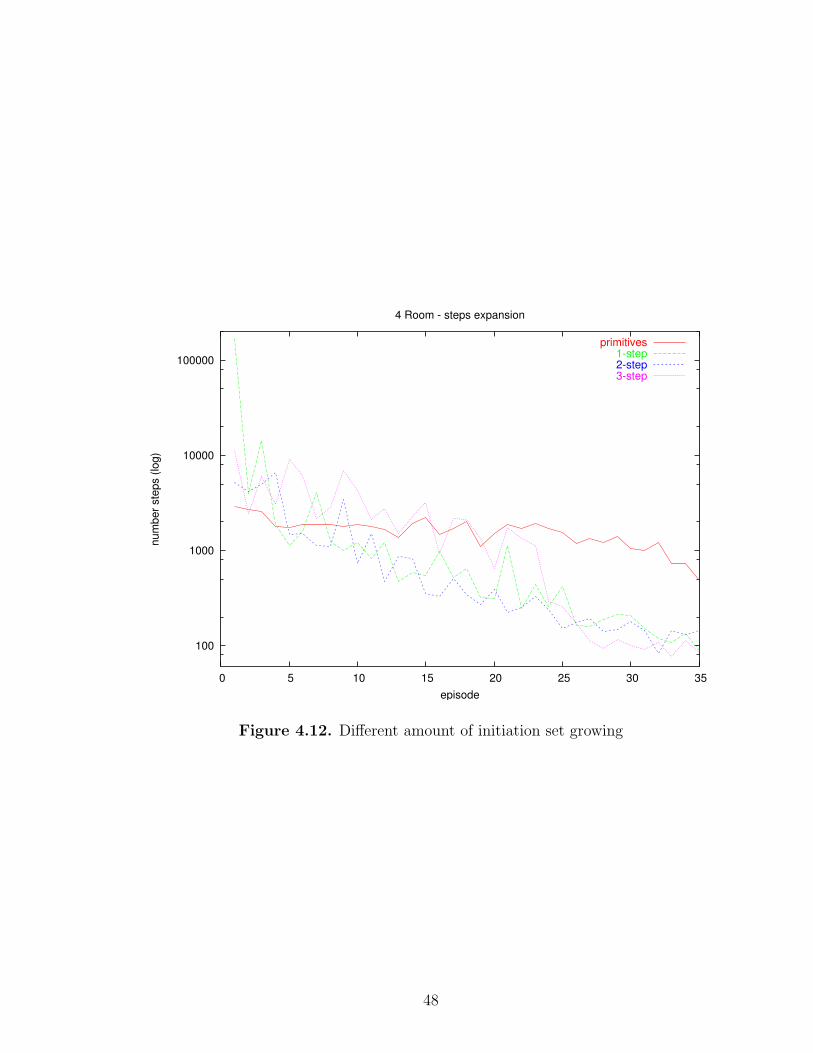
100

1000

10000

100000

0 5 10 15 20 25 30 35

num

ber s

teps

(log

)

episode

4 Room - steps expansion

primitives1-step2-step3-step

Figure 4.12. Different amount of initiation set growing

48

10

100

1000

10000

0 5 10 15 20 25 30 35 40

num

ber s

teps

(log

)

episode

4 Room - backwards

primitives2-step

2-step + backwards

Figure 4.13. Second Algorithm with and without reversed actions

step growing, but also not by much. In the end, the options found by growing the

initiation sets by two steps are the best compromise between increasing the initiation

set size of the options and maintaining the focus on relevant parts of the state space.

In general, however, the algorithm seems robust with respect to this setting.

Figure 4.13 shows the performance of a learner using options that were found when

the states on a trajectory after the subgoal were included in the options’ initiation sets

and the performance of a learner using options where such states where not included

in the initiation set. Performance of the learners is similar. However, including the

states following a subgoal in the initiation set does speed up learning slightly in the

first few episodes, after which the learners perform identically.

Since the cost of the upfront exploration phase is a major Achilles heel, experi-

ments with reduced training during this phase were performed. This can also give

49

100

1000

10000

100000

0 10 20 30 40 50 60 70 80

num

ber s

teps

(log

)

episode

4 Room - reduced quality trials

primitives2-step back

2-step back fewer trajectories2-step back fewer training

Figure 4.14. Second Algorithm under reduced experience

50

some insights into how difficult it would be to use real trajectories, which might not

all be generated by good policies. Another way to reduce the upfront cost is to reduce

the number of tasks chosen. Instead of .25% of all tasks, only .16% of all possible

tasks were tried. In order to give the algorithm the best possible conditions, the

states after the peak of a goal candidate were added to the initiation set, which was

possible because this is a symmetric environment. Furthermore, two step growing

was used, since this seemed the optimal setting.

As expected, when decreasing the amount of experience in the exploration phase,

the quality of the options found decreases as well (Figure 4.14). However, it is worth-

while noting that decreasing the number of tasks only results in a soft degradation of

the quality of the options found. This is probably due to the fact that the agent was

not covering the state space evenly enough and the eight options that it found were

overly concentrated in one area. On the other hand, when each task was only poorly

learned, the quality of the options dramatically decreased. One possible explanation

is that the trajectories used for mining, based on poorly learned policies, were near

random and no useful data could be extracted.

This has interesting implications for a hypothetical, future on-line version of our

option discovery algorithm, which finds options as it learns tasks. It would be possible

to find options right away, as long as it does not find too many options that overlap in

the area of the original trajectories. However, it should only include the trajectories

and look for options, once the task has been properly learned, since the stochasticity

of the episodes when the task has not yet been learned well will dramatically impact

the quality of the options found negatively.

A variant of McGovern’s algorithm was tried, too. As discussed in section 4.3,

the start states for McGovern’s option discovery algorithm were moved around in

order to facilitate the discovery of options that do not lie on the path of only one

particular task. However, as it turned out, after the first start-goal combination was

51

0

2000

4000

6000

8000

10000

12000

14000

16000

0 10 20 30 40 50 60

num

ber s

teps

episode

4 Room - Amy modified

primitivesmcgovern original

mcgovern reduced

Figure 4.15. McGovern’s Algorithm when moving goal around

52

learned (and a few options were found), moving the start state around did not cause

the algorithm to find more options. It seemed like the diverse-density statistic was

saturated. In an attempt to help McGovern’s algorithm, the start state was moved

much quicker (after only 50 episodes instead of 200).

Here are the results of moving the start states around more quickly for McGovern’s

algorithm. Unfortunately, as can be seen in Figure 4.15, this did not lead to an

improvement of the option set. Quite the contrary, the quality of the option sets

found was much worse and impeded the learning of the agent that used these options.

4.6 Directed Exploration with Intra Option Q-Learning

When analyzing the experiments in section 4.5 for the 4 Room environment, we

noticed that in up to three out of 30 experiments that were averaged to produce the

graphs, there were extreme outliers with 600000 to several million steps per episode.

These outliers were removed from the graphs shown above, because they made any

kind of analysis of the performance of the algorithms futile and did not represent the

true performance of the algorithms. Yet, if these algorithms were used in practice,

the issue of occasional poor performance would have to be addressed.

Analysis of the experiments showed that these outliers happened when there were

large regions in the state space which were part of the initiation sets of five or more

options and the subgoals of these options would take the learner away from the goal

of the evaluation task. On the first few episodes then, when the state-action values

were still zero for almost all states and random actions were picked, with probability

of more than 0.5 the agent would pick an action that takes it away from the goal

state. In such cases, an exponential number of time steps before reaching the goal is

to be expected as is documented in the literature [34][35].

In an attempt to avoid this exponential blow-up, algorithms for recency based

directed exploration presented by Thrun [31] were adapted to state-action value based

53

learning in the spirit of Rich Sutton’s work [27]. Instead of associating a time stamp

with each state, a time stamp is associated with every state-action pair. When

greedily selecting which action to pick, the value of each state-action pair is calculated

as follows:

eval(s, a) = Q(s, a) + δ ·√

t− t(s, a) (4.1)

where δ is a weighing parameter that weighs how important exploration is, t is the

current time stamp and t(s, a) is the time at which (s, a) (action a in state s) was

visited. ε-greedy action selection was then used with respect to this value instead of

the original state-action value function.

Care has to be taken when to update the time stamp t(s, a) while executing

an option. Clearly, this depends on the learning algorithm used since Intra Option

Q-Learning and SMDP Q-Learning update different state-action values at different

times. We use directed exploration with Intra Option Q-Learning and update the

time stamp of the primitive action executed at every time step, even when an option

is being executed, since the value for the primitive action is updated nonetheless.

Additionally, when executing an option, at every time step the time stamp of the

option for the state visited is updated. No other option time stamps are updated.

Since using directed exploration also improves the performance of the learner using

primitive actions only, experiments measuring the impact of directed exploration on

learning with primitives only were also run. The results for the 4 Room environment

are shown in Figure 4.16. They show that there is a definite improvement when using

directed exploration with primitive actions, and it is robust toward the setting of the

directed exploration weight. However, it also results in an exploratory policy, which

levels off at a worse level. Even once the optimal action-values are found, the learner

will not always take the optimal action, since sometimes the action was just taken

54

0

500

1000

1500

2000

2500

3000

3500

0 20 40 60 80 100

num

ber s

teps

episode

4 Room - directed exploration primitives

primitivesprimitives direx 0.005

primitives direx 0.05primitives direx 0.1

Figure 4.16. Directed Exploration with primitive actions only

55

100

1000

10000

0 20 40 60 80 100 120 140 160

num

ber s

teps

(log

)

episode

4 Room - directed exploration options

primitivesoptions

options direx 0.005options direx 0.05

options direx 0.1

Figure 4.17. Directed Exploration with found options

56

and other actions will seem more favorable, because they were not taken for a long

time.

Figure 4.17 shows the results of using the found options, including those that cause

severe outliers in the performance of the agent. When adding directed exploration, the

agent successfully avoids the exponential blow up in the first few episodes. Instead of

requiring over 200000 steps on average, it now performs about as well as the primitives.

While this is an impressive improvement, it is still disappointing since, on average,

using the found options will not improve performance over using only primitives.

The improvements due to options in 28 out of 30 experiments are nullified by the bad

performance of the outliers. Furthermore, using directed exploration severely reduces

the performance of the learner in the end. This is likely caused by the fact that once

in a while, when the learner has used all the primitive actions in a particular state

recently, it uses an option that takes it far away. However, even though the graph

is a bit deceiving due to the logarithmic scale on the y-axis, the penalty in the end,

especially when using a weight of 0.005 or 0.05 for the exploratory bonus, is much

smaller than the upfront penalty incurred in the first 30 trials when not using directed

exploration.

Overall, using directed exploration has dramatically reduced the penalty of having

poor option sets, however this improvement is still not satisfactory and is further

lessened by the reduced quality of the final policy. A better solution to the problem

of occasionally having poor option sets would be to incorporate the insights gained

from these experiments and incorporate them into a future option discovery algorithm

that tries to reduce overlap in the initiation sets of options.

4.7 Combined SMDP+Intra Option Q-Learning

In the following series of experiments the different properties of three different

option learning algorithms are explored. The learning algorithms are tried on all four

57

100

1000

0 10 20 30 40 50 60

num

ber s

teps

(log

)

episode

Empty Room - learning algos - random options

primitivesrandom smdprandom intra

random combined

Figure 4.18. Learning algorithms with random options in the Empty Room envi-ronment

environments. Two different option sets were used, the random options as well as the

found options from the second option discovery algorithm.

4.7.1 Grid World Environments

Figure 4.18 shows the weaknesses and strengths of the two conventional learning

algorithms, SMDP Q-Learning and Intra Option Q-Learning, in the Empty Room.

While SMDP Q-Learning initially learns faster, it converges much slower than Intra

Option Q-Learning. This is due to the fact that once an option has been useful,

it will always be preferred over the primitive actions, since their values will not be

updated and it will take a long time before values will have been back propagated

through the primitive action’s selection by exploratory action choice. Clearly, the

combination algorithm combines the best of both worlds. It outperforms the SMDP

58

100

1000

0 5 10 15 20 25 30 35 40

num

ber s

teps

(log

)

episode

Empty Room - learning algos - found options

primitivesoptions smdpoptions intra

options combined

Figure 4.19. Learning algorithms with found options in the Empty Room environ-ment

59

100

1000

10000

100000

1e+06

0 10 20 30 40 50 60 70 80

num

ber s

teps

(log

)

episode

4 Room - learning algos - random options

primitivesrandom smdprandom intra

random combined

Figure 4.20. Learning algorithms with random options in the 4 Room environment

Q-Learner in the initial learning and converges to a policy that is close to the Intra

Option Q-Learning policy.

When using the found options (Figure 4.19), Intra Option Q-Learning learns about

as fast as SMDP Q-Learning and also converges to a better policy. The combined

learning algorithm performs comparably to the Intra Option Learning algorithm and

therefore performs better or at least as good as the best of the two older learning

algorithms in the Empty Room environment.

In the more complicated 4 Room environment, the picture is not as clear for the

random options (Figure 4.20). Again, Intra Option Learning is initially slower in

the original learning phase, but then converges much faster than SMDP Q-Learning.

However, the combined learning algorithm is not quite as fast a SMDP Q-Learning in

the initial learning phase. It starts breaking away from the Intra Option Q-Learning

60

100

1000

0 10 20 30 40 50 60 70

num

ber s

teps

(log

)

episode

4 Room - learning algos - found options

primitivesoptions smdpoptions intra

options combined

Figure 4.21. Learning algorithms with found options in the 4 Room environment

61

100

1000

10000

0 5 10 15 20 25 30 35 40 45 50

num

ber s

teps

(log

)

episode

No Doors - learning algos - random options

primitivesrandom smdprandom intra

random combined

Figure 4.22. Learning algorithms with random options in the No Doors environment

algorithm around the same time as SMDP Q-Learning (around 18 episodes) and only

stabilizes to a good policy after 35 episodes (instead of 30 episodes for SMDP Q-

Learning). In the end it starts to level off at a policy that is in between the quality

of the SMDP Q-Learning policy and the Intra Option Q-Learning policy. Overall, it

is a positive compromise between the two conventional learning algorithms.

Figure 4.21 shows the performance of the learning algorithms with found options.

There is again a performance difference between SMDP Q-Learning and Intra Option

Q-Learning. Intra Option Q-Learning, while clearly using the options to improve

learning over learning with primitive actions, is not quite as fast as SMDP Q-Learning.

However, the combined learning algorithm proves to be the best of both and even

outperforms SMDP Q-Learning in the initial learning speed while leveling off at a

good policy, similar to the Intra Option Q-Learning algorithm.

62

0

500

1000

1500

2000

2500

0 5 10 15 20 25 30 35 40 45 50

num

ber s

teps

episode

No Doors - learning algos - found options

primitivesoptions smdpoptions intra

options combined

Figure 4.23. Learning algorithms with found options in the No Doors environment

63

0

500

1000

1500

2000

0 5 10 15 20 25 30 35 40 45 50

num

ber s

teps

episode

Taxi Domain - learning algos - random options

primitivesrandom smdprandom intra

random combined

Figure 4.24. Learning algorithms with random options in the Taxi environment

In the No Doors environment, both Intra Option Q-Learning and SMDP Q-

Learning perform equally well. The combined learning algorithm is quite a bit better

than the conventional learning algorithms (Figure 4.22)

When looking at the performance of the learners using found options, the picture

is much less interesting. All three learners learn about equally fast. Only SMDP

Q-Learning, again, levels off too soon (Figure 4.23).

4.7.2 Taxi World Environment

The influence of the three learning algorithms on learning in the taxi domain

when using random options is not very clear (Figure 4.24). The difference between

the different learning algorithms are not much bigger than the 95% confidence in-

tervals. Only the combined learning algorithm slightly outperforms the conventional

64

0

500

1000

1500

2000

0 5 10 15 20 25 30 35 40 45 50

num

ber s

teps

episode

Taxi Domain - learning algos - found options

primitivesoptions smdpoptions intra

options combined

Figure 4.25. Learning algorithms with found options in the Taxi environment

65

-45000

-40000

-35000

-30000

-25000

-20000

-15000

-10000

-5000

0

0 5000 10000 15000 20000 25000 30000 35000

cum

ulat

ive

rew

ard

number steps

Taxi Domain - learning algos - cumulative reward

options smdp

options combined

random combined

options intra

random intraprimitives

random smdp

Figure 4.26. Learning algorithms compared by cumulative reward in the Taxi envi-ronment

66

algorithms and approaches the optimal policy much faster than the Intra Option

Q-Learning algorithm

With found options (Figure 4.25), the picture is already much clearer. Both SMDP

Q-Learning and the combined learner clearly outperform the Intra Option Q-Learning

based learner.

Figure 4.26 compares the performance of all learning algorithms with both ran-

dom and found options in the taxi world under consideration of the rewards received

as well as the learning speed. With random options, Intra Option Q-Learning and

SMDP Q-Learning perform about equally well and are comparable to learning with

primitives alone, mirroring the results in Figure 4.24. However, both incur more neg-

ative reward than learning with primitives only. Something that was not apparent

from the previous graph, is that the combined learning algorithm using random op-

tions performs quite well, outperforming even found options used by Intra Option

Q-Learning, both with respect to number of steps (speed of learning) and reward re-

ceived (wrong actions taken). By far the best results are obtained when using SMDP

Q-Learning or the combined learner on the found options. They not only outperform

Intra Option Q-Learning on the same options, but also the best result with random

options by a large margin, both with regard to speed of learning and number of wrong

actions taken.

67

CHAPTER 5

CONCLUSION

In this thesis we have introduced several algorithms that enrich the options frame-

work. The main algorithms allow for the automatic discovery of useful options for

goal-directed tasks. In a variety of experiments, we have shown that both algorithms

find useful options that speed up learning significantly on new tasks and outperform

options found by an existing algorithm. It is worth noting that this earlier algorithm

makes a different set of assumptions - it is an on-line algorithm and can be applied

in situations in which the algorithms presented here cannot be applied. Both option

discovery algorithms presented in this work are batch algorithms. The second new

algorithm makes fewer assumptions, which enables it to serve as the basis for a fu-

ture on-line algorithm. Preliminary experiments were also conducted that show the

performance of the second algorithm in conditions similar to on-line learning. We

believe that these experiments and the second algorithm presented here can be used

as a basis for an algorithm that is specifically designed as an on-line option discovery

algorithm.

Additionally, we introduced a novel learning algorithm for the options framework,

which combines the best of SMDP Q-Learning and Intra Option Q-Learning, two

commonly used algorithms. Empirically, the new algorithm performs better or com-

parable to the best of the two previous algorithms under a variety of conditions. We

believe this to be a significant contribution to the options framework.

There are several possibilities for future work related to the option discovery al-

gorithms. First of all, the second algorithm presented here could serve as the basis

68

for an on-line algorithm. Part of the challenge for this new algorithm is to overcome

the requirements for a large batch of trajectories and to use trajectories from poorly

learned policies, as they frequently occur in the early stages of learning.

Another open issue is how to guard against adverse option sets which can cause

an exponential increase in the number of steps required to learn a task. A possible

venue to eliminate this problem at the root would be to change the selection criteria

for the options, once all candidates are found.

69

BIBLIOGRAPHY

[1] David Andre and Stuart J. Russell. Programmable reinforcement learning agents.In Advances in Neural Information Processing Systems, volume 13, 2000.

[2] David Andre and Stuart J. Russell. State abstraction for programmable rein-forcement learning agents. In Proceedings of the Eighteenth National Conferenceon Artificial Intelligence, pages 119–125, 2002.

[3] Steven J. Bradtke and Michael O. Duff. Reinforcement learning methods forcontinuous-time Markov decision problems. In G. Tesauro, D. Touretzky, andT. Leen, editors, Advances in Neural Information Processing Systems, volume 7,pages 393–400. The MIT Press, 1995.

[4] Thomas G. Dietterich. Hierarchical reinforcement learning with the MAXQ valuefunction decomposition. Journal of Artificial Intelligence Research, 13:227–303,2000.

[5] Thomas G. Dietterich. An overview of MAXQ hierarchical reinforcement learn-ing. Lecture Notes in Computer Science, 1864:26–44, 2000.

[6] Thomas G. Dietterich. State abstraction in MAXQ hierarchical reinforcementlearning. In Advances in Neural Information Processing Systems 12, pages 994–1000, 2000.

[7] Bruce L. Digney. Emergent hierarchical control structures: Learning reac-tive/hierarchical relationships in reinforcement environments. In Proceedingsof the 4th International Conference of Simulation of Adaptive Behavior, pages363–372, 1996.

[8] Bruce L. Digney. Learning hierarchical control structure for multiple tasks andchanging environments. In From animals to animats 5: The fifth conference onthe Simulation of Adaptive Behavior, 1998.

[9] Chris Drummond. Composing functions to speed up reinforcement learning in achanging world. In European Conference on Machine Learning, pages 370–381,1998.

[10] Chris Drummond. Accelerating reinforcement learning by composing solutionsof automatically identified subtasks. Journal of Artificial Intelligence Research,16:59–104, 2002.

70

[11] Fikes, Hart, and Nilsson. Learning and executing generalized robot plans. Arti-ficial Intelligence, 3:251–288, 1972.

[12] Bernhard Hengst. Discovering hierarchy in reinforcement learning with HEXQ.In Proceedings of the Nineteenth International Conference on Machine Learning,pages 243–250, 2002.

[13] Glen A. Iba. A heuristic approach to the discovery of macro-operators. MachineLearning, 3:285–317, 1989.

[14] Tommi Jaakkola, Michael I. Jordan, and Satinder P. Singh. Convergence ofstochastic iterative dynamic programming algorithms. In Jack D. Cowan, Ger-ald Tesauro, and Joshua Alspector, editors, Advances in Neural InformationProcessing Systems, volume 6, pages 703–710. Morgan Kaufmann Publishers,Inc., 1994.

[15] J.E. Laird, P.S. Rosenbloom, and A. Newell. Chunking in soar: The anatomy ofa general learning mechanism. Machine Learning, 1:11–46, 1986.

[16] O. Maron. Learning from Ambiguity. PhD thesis, Massachusetts Institute ofTechnology, 1998.

[17] O. Maron and T. Lozano-Perez. A framework for multiple-instance learning.In M. I. Jordan, M. J. Kearns, and S. A. Solla, editors, Advances in NeuralInformation Processing Systems, volume 10, pages 570–576, 1998.

[18] Amy McGovern. Autonomous Discovery Of Temporal Abstractions From Inter-action With An Environment. PhD thesis, University of Massachusetts Amherst,2002.

[19] Amy McGovern and Andrew G. Barto. Automatic discovery of subgoals inreinforcement learning using diverse density. In Proc. 18th International Conf.on Machine Learning, pages 361–368. Morgan Kaufmann, San Francisco, CA,2001.

[20] Amy McGovern and Richard S. Sutton. Macro-actions in reinforcement learn-ing: An empirical analysis. Technical Report 98-70, University of MassachussetsAmherst, 1998.

[21] Ronald Parr and Stuart J. Russell. Reinforcement learning with hierarchies ofmachines. In Michael I. Jordan, Michael J. Kearns, and Sara A. Solla, editors,Advances in Neural Information Processing Systems, volume 10. The MIT Press,1997.

[22] Doina Precup. Temporal Abstraction in Reinforcement Learning. PhD thesis,University of Massachusets Amherst, 2000.

71

[23] Balaraman Ravindran and Andrew G. Barto. Relativized options: Choosing theright transformation. In Proceedings of the Twentieth International Conferenceon Machine Learning, 2003.

[24] Balaraman Ravindran and Andrew G. Barto. Smdp homomorphisms: An alge-braic approach to abstraction in semi markov decision processes. In Proceedingsof the Eighteenth International Joint Conference on Artificial Intelligence, 2003.

[25] Martin Stolle. Source code for master’s research. Internet/WWW.http://rl.cs.mcgill.ca/˜mstoll/masters-src.tar.gz.

[26] Martin Stolle and Doina Precup. Learning options in reinforcement learning.Lecture Notes in Computer Science, 2371:212–223, 2002.

[27] Richard S. Sutton. Integrated architectures for learning, planning, and reactingbased on approximating dynamic programming. In Proceedings of the SeventhInternational Conference on Machine Learning, pages 216–224, 1990.

[28] Richard S. Sutton and Andrew G. Barto. Reinforcement Learning: An Introduc-tion. MIT Press, Cambridge, MA., 1998.

[29] Richard S. Sutton, Doina Precup, and Satinder Singh. Intra-option learningabout temporally abstract actions. In Proc. 15th International Conf. on MachineLearning, pages 556–564. Morgan Kaufmann, San Francisco, CA, 1998.

[30] Richard S. Sutton, Doina Precup, and Satinder P. Singh. Between MDPs andsemi-MDPs: A framework for temporal abstraction in reinforcement learning.Artificial Intelligence, 112(1-2):181–211, 1999.

[31] Sebastian B. Thrun. Efficient exploration in reinforcement learning. TechnicalReport CMU-CS-92-102, Carnegie Mellon Uniersity, Pittsburgh, Pennsylvania,1992.

[32] Sebastian B. Thrun and Anton Schwartz. Finding structure in reinforcementlearning. In G. Tesauro, D. Touretzky, and T. Leen, editors, Advances in NeuralInformation Processing Systems, volume 7, pages 385–392. The MIT Press, 1995.

[33] Christopher J. C. H. Watkins. Learning from delayed rewards. PhD thesis,Cambridge University, 1989.

[34] Steven D. Whitehead. A complexity analysis of cooperative mechanisms in rein-forcement learning. In Proceedings of the Ninth National Conference on ArtificialIntelligence, pages 607–613, 1991.

[35] Steven D. Whitehead. Complexity and cooperation in q-learning. In MachineLearning: Proceedings of the Eighth International Workshop, pages 363–367,1991.

[36] Marco Wiering and Jurgen Schmidhuber. HQ-learning. Adaptive Behavior,6(2):219–246, 1997.

72