nber working paper series on the monetization of … · suggests that monetization matters mostly...

NBER WORKING PAPER SERIES

ON THE MONETIZATION OF DEFICITS

Alan S. Blinder

Working Paper No. 1052

NATIONAL BUREAJJ OF ECONOMIC RESEARCH1050 Massachusetts Avenue

Cambridge MA 02138

December 1982

Revised version of a paper presented at the conference on "TheEconoj,jc Consequences of Government Deficits" at WashingtonUniversity, st. Louis, Missouri,

October 29—30, 1982. I thankLeonard Nakamura forresearch assistance, the National ScienceFoundation for research

support, and Scott Hem, Dwight Jaffee,Michael Levy, Jorge de Macedo, Hyman Minsky, Franco Modigliani,Joseph Stiglitz, John Taylor, and Burton Zwiclc for helpful commentsand suggestions on an earlier draft. The research reported here ispart of the NBER's research

program in Economic Fluctuations.AnyOpinions expressed are those of the

author and not those of theNational Bureau of Economic Research.

NBER Working Paper #1052December 1982

On the Monetization of Deficits

ABSTRACT

Whether or not a deficit ismonetized is often thought to have important

macroeconomic ramifications. This paper is organized around two questions.

The first is: Doesmonetization matter?, or more specifically, For a given

budget deficit, do nominal or real variables behave differentlydepending

on whether deficits are monetizedor not? Virtually all macro models give

an affirmative answer. Aftersorting out some theoretical issues that

arise in a dynamiccontext, i present some new time series evidence which

suggests that monetization mattersmostly for nominal variables.

The second question is: What factors determine how much monetization

the Federal Reserve will do?After discussing some normative rules, I

offer a game—theortargument to explain why a central bank may choose not

to monetize deficits at all and may even contract bank reserves when the

government raises its deficit. Theempirical work turns up a surprisingly

systematic link between budget deficitsand growth in reserves. This

relationship suggests that the FederalReserve monetizes deficits less when

inflation is high and whengovernment purchases are growing

rapidly.

Alan S. Blinder

Department of EconomicsPrinceton UniversityPrinceton, NJ 08544

(609) 452—4010

A government deficit is said to be 'moneti-ed" when the

central bank purchases the bonds that the government issues to

Because of the central bank's balance sheet

urchases increase bank reserves unless offset

tions. By contrast, new government debt

vate parties does not increase bank reserves.

difference, whether or not a deficit is

en thought to have important macro— economi

And there is considerable evidence that thi

orrect.-

is organized around two questions; Does

ter? and, What factors determine how much

Federal Reserve will do? Both of these

een asked before, and my answers will be less

My aims are more modest: to bring a bit more

evidence to bear on the issues and to add

I takes up the first question: For a given budget

deficit, will nominal or real variables behave differently

depending on whether the new bonds are purchased by the central

bank or by the public? Notice that this is basically the same

as asking; Do open—market operations matter? Virtually all

macro models give an affirmative answer. But some recent

theoretical developments, which I review, suggest that the

issue is a good deal more complicated than indicated by simple

models like the quantity theory or IS—LM. After sorting out

cover its deficit.

identity, such p

by other transac

purchased by pri

Because of this

monetized is o-ft

ramifications.

supposition is c

This paper

monetization mat

monetization the

questions have b

than startling.

c

5

the discu

Sect

ssi on.

ion

a few new thoughts to

some theoretical issues that arise in a dynamic context, I

present some new time series evidence which supports the old

idea that monetization matters.

Section II addresses the second issue: How does the Fed

decide how much of each deficit to monetize? First, some

normative rules dictating how the Fed should make this decision

are presented and brie-fly evaluated. Then a gametheoretic

argument is offered to explain why a central bank with

discretionary authority may choose not to monetize deficits at

all and mayinstead do the opposite, i.e., contract bank

reserves when the government raises its deficit! Finally, I

offer some empirical evidence suggesting that there is a

systematic link between budget deficits and growth in reserves.

This relationship suggests that the Federal Reserve moneti:es

deficits less when inflation is high and when government

purchases are growing rapidly.

I. DOES MONETIZATION MATTER?

Elementary macro models, including both the quantity

theory and IS—LM, suggest that budget deficits have a greater

effect on aggregate demand if they are monetized.

This difference is extreme under the crude quantity

theory. Obviously, if Py=MV and V is a constant, then deficits

increase nominal demand if and only if they are monetized. <1>

A slightly more sophisticated quantity theory, which recognizes

that nonmonetized deficits raise velocity by raising interest

rates, allows for an effect of deficits on aggregate demand.

But the supposition that the effect of money is greater is

maintained.

Essentially the same conclusion emerges from the fix—

price IS—LM model. Figure 1 shows an initial IS—LM equilibrium

at point A. Higher government spending or a cut in taxes

raises the IS curve to IiSi. If the deficit is not monetized,

the LM curve is unchanged and equilibrium moves to point B;

output rises. But if the deficit is monetized, the LM curve

shifts as well (to L1M1) and output increases even more (point

C).

This is all very simple, but it leaves out much. Among

the important omissions are:

- (1) wealth effects on the IS and/or LM curves and the

resulting dynamics that are implied by the government budget

C

-C,

-1

7

/ Lc

G

LA(

constraint;

PAGE 4

(2) changes on

higher or lower interest

(3) expectation

financing decision (which

between the real interest

the supply side of the economy as

rates affect investment;

al effects set up by the government's

, among other things, intervene

rate and the nominal interest rate).

The next three subsections take up each of these in turn.

sellinghigh— p

where H is hi

taken to have

purchases, r

receipts. wri

As Solow

are wealth ef

set up by (1)

viewpoint of

remains stabl

either to the Federal

money) or to the pUblic

1) dH/dt + dB/dt = B

gh— powered money,

zero maturity), 6

is the nominal mt

tten as a function

+ rB — T(V)

of

be financed by

(and hence creating

s publicly—held bonds (here

government

and T is nominal

income.

decade ago

then the

adoxical f

cular, i

cits (wh

, idyn

rom

f theich i

total expenditures

1. WEALTH EFFECTS AND THE GOVERNMENT BUDGET CONSTRAINT

The government budget constraint states that any excess

bonds

owered

C

over total receipts must

Reserve

Bi

is nominal

erest rate,o-f nominal

and I (1973) showed almost a

fects on the IS and LII curves,

lead to results that seem par

static macro models. In parti

e under bond financing of defi

+ there

ami Cs

the

model

s by no

means a sure thing), then the long—run effects of a deficit on

aggregate demand are greater if it is not monetizeth

How can this be true in view of Figure 1? Suppose we add

wealth effects to the analysis and assume that government bonds

are net wealth. <2> Start with the case of bond financing

(point B). The additional wealth represented by the new bonds

augments consumer spending and pushes the IS curve further to

the right. At the same time. however, the LM curve shifts

leftward if there is a wealth effect on the demand for money

<3> The net result of these two wealth effects is clearly to

increase r. But the net effect on V seems to be ambiguous.

However, Solow and I showed (as is obvious) that in a stable

system the net impact of the two wealth effects must increase

income.

The dynamic adjustment proceeds as follows. Each

injection of bonds increases income, and the process continues

(in a stable system) until the induced tax receipts bring the

budget into balance. The dynamics are similar under money

financing, except that each dollar of newly— created money has

an additional liquidity effect on the LM curve which malr:es Y

rise even faster.

Why, then, do bond—financed deficits have larger effects

in the long run? The reason, loosely speaking, is that bond—

financed deficits "last longer." More precisely, bond—financed deficits raise the government's interest expenses

whereas money— financed deficits reduce them. Thus, while each

$1 billion bond issue expands V by less than a $1 billion issue

In (2).(3), rthe mul

Of

under b

return.

fi nancing.

we know that the

-financing? Set

total derivative

(3) dY/dG =

both r and B are

is driven down by

tiplier in (2) ex

course, all this

0th methods of •fi

It also ignores

net result

1) eqL(al to

with respect

new paper

rise in B

(1 + d(rB

leaves B

(1 + B(dr/dG)).

by the increase

ase in M. It fol

multiplier in (3)

hat the ec

matter tu

ons, the be

assets

greater

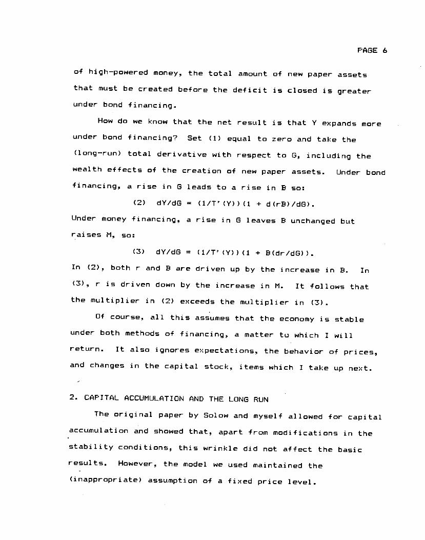
2. CAPITAL CCUf1ULTION IND THE LONG RUN

The original paper by Solow and myself allowed -For capital

accumulation and showed that, apart from modifications in the

stability conditions, this wrinkle did not affect the basic

results. However, the model we used maintained the

(inappropriate) assumption of a fixed price level.

of high—powered money, the total amount

that must be created before the deficit

PAGE 6

of new paper

is closed is

under bond

How do

under bond

(1 ong—run)

wealth effe

+ i rianci ng,

is that V expands

zero and take the

to 6, including

cts of the cr

a rise in 6 1

(2) dY/dG =

Under money -financing,

more

the

raises M, so:

assets. Under bond

so:

/dG).

unchanged but

eation of

eads to a

(l/T' (Y))

a rise in 6

(l/T' CV))

driven up

the incre

ceeds the

assumes t

nancing, a

e<pectati

in B.

1 ows

In

that

and changes in the capital stock, items which

onomy is stable

which I will

havior of prices,

I take up next.

Fortunately, subsequent work established very similar

conclusions in models which deal more satisfactorily with the

price level. <4> -

If the labor force and technology are more or less

exogenous, then the long—run effects of monetization depend on

how the capital stock reacts. Neoclassical growth models lead

to the supposition that money financing of deficits is better

for capital formation than bond financing, <5> but adding even

a minimal amount of complexity to standard macro models

introduces enough ambiguity so that even this intuitive

conclusion cannot be derived.

The ambiguities arise from the interaction of wealth

effects and interest elasticities, neither one of which can be

ignored without assuming away the problem. Consider, as an

example, the following simple IS—LM model augmented to include

wealth effects:

(4) y = c(y—t(y). a) + i(r—ir,K) + g

(5) M/P = L(r, y, a)

(6) a = K + M/P + B/P

- (7) dtl/dt + dB/dt = P(g — t(y)) + rB

(8) (1/P)(dP/dt) u + h(y — F(K))

(9) dK/dt = i(r—n,K)

Equations (4) and (5) are IS and LM curves augmented to include

-real wealth, a, which is defined in (6). Here r denotes the

nominal interest rate and iT the expected rate of inflation.

The difference between M and H is ignored. Equations (7)—(9)

give the dynamics of the three state variables: P. K, and

either M or B. Equation (7) is the government budget

constraint; equation (8) is an expectational Phillips curve;

and equation (9) updates the capital stock.

The signs of most of the short— run comparative static

multipliers implicit in (4)—(6) can be determined with only the

usual qualitative assumptions. An important exception.

however, is dr/dM which., even ignoring possible effects of M on

expected inflation (about which more later), has the sign of:

CaLy - (1_L.a)[1_c(1._tI')]an expression which is negative in the absence of wealth

effects, but ambiguous in their presence. The economics behind

this ambiguity is quite simple. Normally, an increase in II

lowers interest rates by shifting the LM curve to the right.

But the wealth effects of an injection of money shift the UI

curve to the left and the IS curve to the right, thereby

pushing up interest rates. These wealth effects could

conceivably be strong enough to offset the original effect of .M

on the LM curve.

- As might be surmised, this ambiguity is devastating to

long—run analysis where primary attention focuses on the

behavior of the capital stock. If we do not know in which

direction II pushes r, then we certainly will not be able to

• tell in which direction it pushes K, In fact, none of the

long—run comparative static derivatives (obtained from

equations (4>—() and from equations (7)—(9) set equal to zero)

are of determinate sign unless wealth effects are assumed away.

But this is not a legitimate way out of the indeterminacy

because Solow and I (1973) showed years ago that wealth effects

are intimately involved in the stability conditions. <6>

The conclusion, unfortunately, seems to be that theory

will tell us little about the long—run consequences of the

monetization decision. Econometric estimation arid simulation

of quantitative models seem to be the only ways out.

3. THE GOVERNMENT BUDGET CONSTRAINT AND EXPECTATIONS

The dynamic constraints across choices of policy mixes set

up by the government budget constraint bring expectaticDnal

issues to the fore.. The identity points out that today's

deficit and monetization decisions have implications for the

feasible set of fiscal—monetary combinations in future periods.

For example, suppose an expansionary -Fiscal policy today

leads to a large deficit that is not monetized. Future

government budgets will therefore inherit a larger burden of

interest payments, so the same time paths of 6, M, and tax

rates will lead to larger deficits. What will the government

do about this? That depends on its reaction function. For

example, large deficits and high interest rates might induce

greater monetary expansion in the future (the possibility

emphasized by Sargent and Wallace (1961)). Alternatively, it

might induce future tax increases (the case stressed by Barro

(1974)), or cuts in government spending (the apparent hope of

Reaganomics). Yet another possibility is that the government

will simply finance the burgeoning deficits by issuing more and

more bonds. <7>

All of these are live options, and have different

implications for the long—run evolution of the economy. In

fact, under rational expectations, they may have different

implications for the state of the economy today.

As an example of a nor-imonetized deficit, consider a tax

cut financed by issuing new bonds. Such a tax cut todayenlarges current and prospective future budget deficits,thereby requiring some combination of the following policyadjustments:

(1) increases in future taxes;(2) decreases in future government expenditures;

(3) increases in future money creation;

(4) increases in future issues of interest— bearing

national debt.

To the extent that the current decisions made by individualsand firms are influenced by their expectations about thefUture, each of these alternatives may have different

implications for the effects o-f the tax cut today.

For example, if people believe that a tax cut financed by

bonds simply reduces today's taxes and raises future taxes inorder to pay the interest on the bonds, then consumption may

not be affected. This is essentially Darro's (1974) argument.

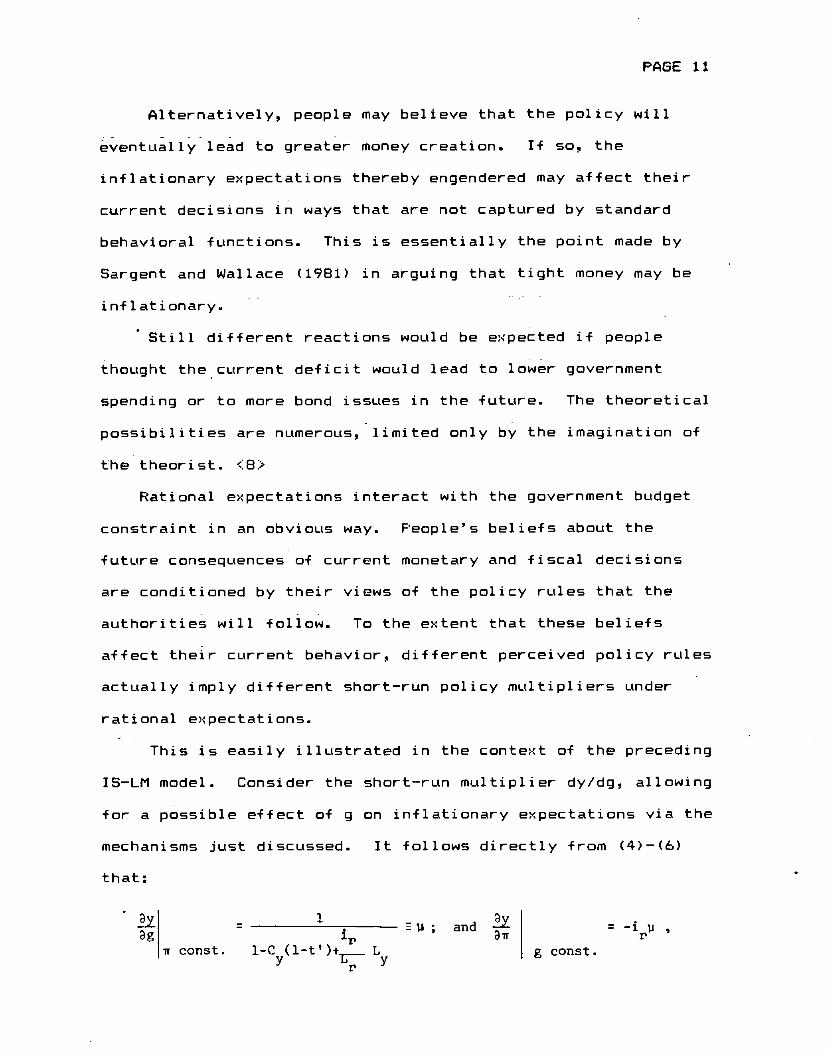
Alternatively, people may believe that the policy will

eventually lead to greater money creation. If so the

inflationary expectations thereby engendered may affect their

current decisions in ways that are not captured by standard

behavioral functions. This is essentially the point made by

Sargent and Wallace (1981) in arguing that tight money may be

inflationary.

Still different reactions would be expected if people

thought the current deficit would lead to lower government

spending or to more bond issues in the future. The theoretical

possibilities are numerous, limited only by the imagination of

the theorist. <8>

Rational expectations interact with the government budget

constraint in an obvious way. Feople's beliefs about the

future consequences of current monetary and fiscal decisions

ar-b conditioned by their views of the policy rules that the

authorities will follow. To the extent that these beliefs

affect their current behavior, different perceived policy rules

actually imply different short—run policy multipliers under

rational expectations.

This is easily illustrated in the context o-f the preceding

IS—UI model. Consider the short—run multiplier dy/dg allowing

for a possible effect of g on inflationary expectations via the

mechanisms just discussed. It follows directly from (4)—(6)

that:

•

•••

1E

; and = —lu ,

,r const. 1_C(1_t)÷.1 L g const.

and from the chain rule that:

dy/dg = + C dvr/dg) C3g h

¶ g

The first term is the standard (positive) government spending

multiplier in IS—LM analysis. The second term is the product

of a positive effect of inflationary expectations on output and

an effect of g on i which depends on the factors enumerated

above. If it is positive, as seems likely, then expectational

effects make the short—run multiplier larger. But it is

conceivable that dir/dg could be zero or even negative.

A key question for policy formulation is: how important

are these expectational effects in practice? This seems to

depend principally on how forward—looking urrent economic

decisions really are.

Take the tax cut example again. Under the pure permanent

income hypothesis (PIH) only the present discounted value of

lifetime alter—tax income flows affects current consumption.

<9> So expectations about future budget policy should haveiniportant effects on current consumption. But if short-

sightedness, extremely high discount rates, or capital market

imperfections effectively break many of the links between the

future and the present, then current consumption may be rather

insensitive to these expectations and rather sensitive to

current income. Even under fully rational expectations and the

pure PIH, consumption may depend largely on current income if

the stochastic process generating income is highly serially

correlated. These are issues about which knowledge is

accumulating; but much remains to be learned. The evidence to

date does not lead to the conclusion that long—term

expectations rule the roost. <10>

The other two places where expectations about future

fiscal and monetary policies might have significant effects on

current behavior are wage and price setting and investment.

Investment, of course, is the quintessential example of an

economic decision which is strongly conditioned by expectations

about the future.. Even Keynes knew this! Eut, once again,

there are some real—world considerations that interfere with

the strictly neoclassical view of investment as the

unconstrained solution to an intertemporal optimization

problem. One is that capital rationing may interfere with a

firm's ability to run current losses on the expectation of

future profits. A second is that management may use ad hoc

rules such as the payback period criterion in appraising

investment projects. A third is the emerging "business school'

view that managers are more shortsighted than they "should be"

because they face the wrong incentives. A fourth is that there

may be a strong accelerator element in investment spending,

which ties the current investment decision much more tightly to

the current state of the economy than neoclassical economics

recognizes. As in the consumption example, each of these

rules which are based

as expected future exc

crucial. Aain, this

before we can make any

A word on uncerta

this topic. It seems

uncertainty to their b

policies will be. If

probability distributi

current decisions than

rational expectations

influence does the two—

decision about

date?

current

effects less

important example. Ad

on forward— looking consi

ess demand) make expectat

is an area where we must

definitive Judgments. <11>

inty seems appropriate before leavi

to me that people probably attach g

el iefs about what future government

so, the means of their subjective

ons may have far less influence

the contemporary preoccupation

would suggest. For example, how

week—ahead weather forecast have

PAGE 14

things diminishes the Importance of the future to

decision making and thereby renders expectational

important.

Wage and price setting is another

hoc rules which adjust wages or prices in accor

law of supply and demand," or which are mainly

looking, render expectational effects rather un

dance with "the

backward

important. But

derations (such

ional effectslearn much more

ng

r eat

on theirwith

much

on

whether or not to plan a picnic on a given

your

Similarly, the importance of expectations for macroeconomic

aggregates is diminished by the likelihood that different

people hold different expectations about what future government

policies are likely to be. <12> If some people believe today's

tax cuts signal higher future taxes, some believe they signal

higher future money creation, and some believe they signal

lower future government spending, then expectations about the

future may have meager current effects in the aggregate.

The conclusion seems to be that, while we should not

forget about expectational effects operating through the

government budget constraint, neither should we get carried

away by them. There is no reason to believe that they are the

whole show.

4. NEW TIME SERIES EVIDENCE

The two preceding sec

accumulation and expectati

theoretical discussion of

creates complexities that

in practice. The latter

may be intractable even i

speak for themselves? Th

reliable structural model

enumerated. What I offer

ambitious: some simple t

knowledge of the monetiza

in nominal GNP, real GNP,

The framework for suc

established by

repeated here.

(1)

tions showed that capital

ons considerably complicate

the monetization issue. The

can be handled in principle,

opens up so many possibilities

n principle. Can we let the d

is is hazardous in the absence

embodying many of the effects

in this section is far less

ime series evidence on whether or not

tion decision helps predict movements

and the price level.

h an analysis has been well

), and will not be

however:

to do with

former

but not

that it

at a

of a

it

Granger (1969) and Sims (1972

Two points are worth making,

Granger—causation has nothing

(13) ,Y/Y = a(L)(AV/Y) +

These were estimated on anni.tal fi

maximum lag extending back either

Monetization "does not matter

Predict growth in Y, if the b coef

Analogously, debt

(AR/R> + c(L) (tD/D).

year data, with the

or three years. <13>

that is, fails to help

ients are Jointly

icy "does not matter"

causation in the usual sense. Since it is quite possible,

especially once expectational influences are accounted for.

that the "effect" might precede the "cause," learning that X

Granger—causes V tells us nothing about whether or not V moved

"because of" X. It means that X adds to the ability to

predict Y, no more and no less.

(2) Whether or not X contributes to the ability to

predict Y may depend on what other information is considered.

Thus, for example, it is perfectly possible that X might

Granger— cause V when some other variable, Z, is excluded from

the regression, but fail to Granger—cause V when Z is

included. In this context, I will interpret the question

"Does monetization matter?" as asking whether or not changes

in bank reserves Granger—cause nominal GNF growth (or

inflation) once we control for growth of the national debt.

Letting V denote nominal GNP. R denote bank reserves, D

denote the outstanding stock o-f government bonds (including

the portion owned by the Fed), and denote the first—

difference operator, regressions of the following form were

run I

b CL)

scal

two

I'

ficpol

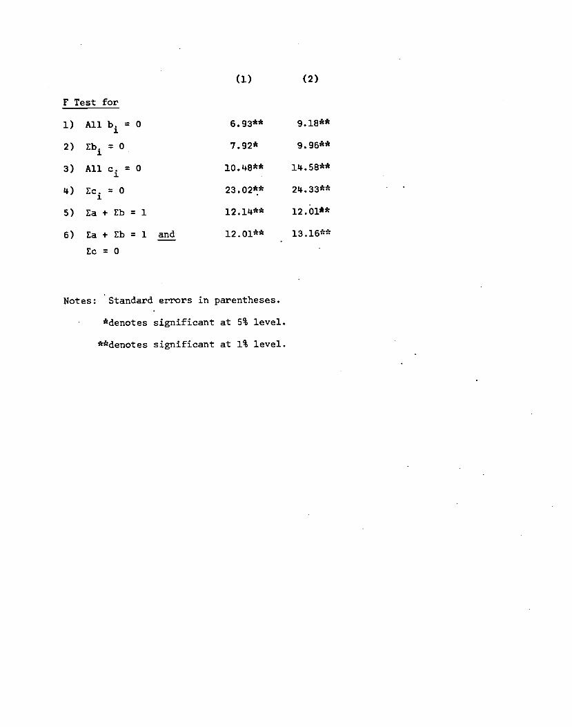
(given monetary policy) if the c coefficients are Jointly

insignificant. Notice that the crude quantity theory suggests

a unitary long—run elasticity for bank reserves and a zero

long—run elasticity for the non—monetized debt, that is:

Sc =0Sa + Sb = 1 and

These hypotheses are all testable by standard F tests.

In estimating (13), D was defined as the increase in

government indebtedness to the public during fiscal year t.

Fiscal, rather than calendar, years were used so as to get a

more accurate measure of the deficit. Budget numbers in the

national income and product accounts (NIPA) differ in several

ways from those in the unified budget, and the deficit series

I used differs further from the unified budget owing to the

activities of off—budget agencies. This suggests a

potentially large slippage between, say, quarterly NIPA

deficit numbers and the true government borrowing

requirement.

In order to use the fiscal year as the unit of time,

quarterly data on adjusted bank reserves, P, <14> and nominal

GNP. V, were put on a fiscal year basis. <15> Results from

estimating equation (13) by ordinary least squares over the

period 1952—1981 appear as regressions (1) and (2) in Table 1.

Roughly speaking, the regressions make it look as if only the

first lag of each variable matters. But, in keeping with the

spirit of this sort of work, the "insignificant" variables

were not dropped.

Table 1

Regressions for Nominal GNP Growth, Fiscal Years 1952-1981

Variable (1) (2)

Constant .068 .052(.015) (.012)

—.536 —.515(.196) (.187)

—.082 .093

(.203) (.125)

— 17't(.133)

.675 .715(.150) (.1146)

(AR/R)2 .186 .116(.212) (.199)

.lL9

(.197)

.3149 .328(.091) (.080)

(D/D)2 .125 . .177(.1114) (.1oL)

(AD/D)3 .161

(.108)

R2 .80 .78

DW 2.16 2.25

Eb..56 .581-Ea.

]

Ec..35 .361-Ea.

)

(].) (2)

F Test for

1) AU b 0 6.93** 9.18**1

2) Eb. = 0 7.92*2.

3) All c = 0 1o.8** lLl 58**1

Li.) Ec. 0 23.02** 2'4.331

5) Za + Eb = 1 l2.lL** 12.Ol**

6) Za + Eb = 1 and 12.0l** l3.l6

Zc=0

Notes: Standard errors in parentheses.

*denotes significant at 5% level.

**denotes significant at 1% level.

debt

ct nom

an aff

change

ci ent.

of the

R/R does

weaker

a, that

the po

the est

oiling +

(F test

elastici

tization

We can,

in national

control

suggest

number

Zero i

whi 1

the

is controlled for

inal GNP growth?

irmative answer,

in reserves has a

More formally, F

table, decisively

not Granger—cause

ypothesis is thats, that reserves

timates are un

elasticity ofis about .57.

er 2), the appr

significantly

matter.

0 LI r 5

helps

Once growth of

. does growth of reserves

The point estimates cert

since in each regression

large and significant

test number 1, reported at the

rejects the null hypothesis

AY/V.

the

have

the b coeffi

g—run effect.

Hard—core monetarism

as can be seen in F—test

the c coefficients are

weaker hypothesis that.

they do not matter in

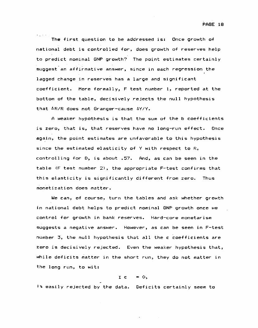
The first question to be addressed is:

PAGE 18

help

ai ni y

the

national

to predi

suggest

lagged

coeffi

bottom

that A

A

is zer

again,

since

contr

table

this

mon e

sum of

no lon

ci en t 5

Once

h

1.

mt

i ma

or

n u

tydoe

of

debt

es

ted

D,

mb

is5

c

favorable to th

V with respectAnd, as can be

opriate F—test

different from

is hypothesis

to R.

seen in the

confirms that

zero. Thus

turn the tables and ask whether growth

to predict nominal GNP growth once we

for growth in bank

s a negative answer.

3, the null hypothesis decisively rejected.

e deficits matter in the

long run, to wit:

Xc

)i easily rejected by the data.

reserves.

However,

s that allEven the

short run

= C),

Deficits certainly seem to

1 conclusion from these regressions is clear:

and nonmonetized deficits are significant

of ubseqLtent C'NP growth.

vious question is whether the debt and reserves

L(sed in Table 1 are mainly predicting movements of

movements of real output. To address this question,

eports the results from regressions analogous to

(13), but using the GNP deflator in place of nominal

The results differ from those obt

in a number of ways, and are far more

quantity—theoretic approach. Unfortu

the case of nominal GF'IP, some of the

we use the regression with three lags

regression with two lags (column 2).

First, the null hypothesis that growth

Contribute to the explanation of inflation

the equation using three lags —— but only

PAGE 19

.tiMtter.

What about the characteristic quantity—theory implication

6).

elasticity of V with respect to R 1S unity?

(in F test number 5), the null hypothesis

ty is unity, i.e. that Za + Eb 1, is

The quantity theory fares no better if it

ude the implication Xc c) (F test number

thatthe long—runj the table shows

that this elasticiclearly rejected.ss extended to md

The overal

both monetized

predi ctors

An ob

variables

.prices or

Table 2 requation

GNP.

ained with nominal GNP

favorable to the

nately, in contrast to

results depend on whether

(column 1) or the

in reserves does

can be rejected in

at the. 57. level of

Table 2

Regressions for Inflation, Fiscal Years 1952-1981

Variable (1) (2)

Constant —.005 —.000(.006) (.006)

(P/P)i 32 .508

(.179) (.173)

—.009 .318(.207) (.182)

.209

(.178)

(.096) (.107)

(R/R)2 -.009 —.099(.102) (.100)

(R/R)3- - .189

(.096)

(D/D)i— .071 — .087(.077) (.075)

(D/D)2 .135 .182(.069) (.063)

.086(AD/D)3

(.06L1.)

.87 .81

DW 1.50 1.5L1

Eb.

1.08 .811_Ea

Ec.: 79 .55

1_Ea

(1) (2)

F Test for

1) All b. = 0 3L7* 2.821

2) Eb. = 0 6.55* 1021

3) All c = 0 3L7* L.23*

I.') Ec. = 0 2.10 1.571.

5) Za+Eb1 .02

6) Ea + Eb = 1 3.25 1.08

and Ec = 0



significance, not at the 17. level. In the equation using two

lags, it cannot be rejected at all. (See F test number 1 at

PAGE 20

Table

in the

2..)

two—lag equation we

the bottom of

Second,

hypothesis

is zero ——

entertain.

equation

Fort un

we use two

cannot even reject the

that the long—run

an hypothesis that

However, we can e

(See F test number

elasticity of

almost rto on

asily reject

2..)

R

atel y,or thre

P with

e would

it in th

depend

For ex

l.ation

e 57..

the other results do

e lags of the variab

debt helps to predi

are contro le for)

respect to

seriously

e three—lag

on whether

ample,

(once

but not the

not

1 es.

ct iad

nf

t th

growth in national

growth in reserves 1

17., level. (F test number 3.) However, the null hypOthesis

that the long—run elasticity of P with respect to D is zero

cannot be rejected. (F test number 4.) The implications that

we associate with the strict quantity theory (see F tests 5

and 6) also cannot be rejected.

Table 3 reports the analogous regressions and F tests

using real GNP in place of nominal GNP. Naturally, the

explanatory power is much lower since we are using nominal

reserves and nominal debt to explain a real variable. In

general, very few significant effects are found.

For e<ample, the hypothesis that growth in reserves does

not help predict real GNP growth can be rejected at the 57.

level in the regression using two lags of each variable. But

it cannot be rejected at the 17. level; and it cannot be

Table 3

___Regressions for Real GNP Growth, Fiscal Years 1952-1981

Variable (1) (2)

Constant .033 .022

(.015) (.013)

—.019 .147

(.209) (.184)

.427 - --.296(.256) (.213)

—.120(.227)

(R/R)i .262 .258- (.187) (.188)

(RfR)_2 —.393 —.450

(.169) (.172)

(R/R)_3 —.198

(.208)

.374 .291

(.152) (.138)

—.203 —.218

(.156) (.124)

—.126(.135)

.36

DW 2.35 2.24

Eb.—.146 —•35

1-Za.)

Ec..06 .131 -Ea.

J

(1) (2)

F Test for

1) All b. = 0 2.56 11.01*1

2) Eb. = 0 1.11 0.6111

3) All c. = 0 2.57 2.351

11) Ec. = 0 0.11 0.1131.



The hypothesis that growth in

real GNP growth cannot be rejected

While the point estimates of

with respect to R are sizeable and

the two versions). neither differs

quantity—theoretic value of zero

estimated long—run elasticity of y

small positive number (.06 and .13

is nowhere near significant (see F

In sum, neither growth

national debt carries much

predicting future real GNF

debt does not help predict

in either regression

the long—run elastici

negative (—.46 and —

significantly -from t

see F text number 2).

with respect to D is

in the two versions),

test number 4).

PAGE 21

rejected at all in the regression using three lags of each

var i ab 1 e.

yty of

..35 in

he

The

a

but

inin bank reser

information th

growth accordi

yes

at

ng

nor growth

iS useful in

to these

equations.. The -fact that both variables were significant

predictors o-f future growth in nominal GNF seems to stem

mainly -from their value in predicting inflation.

== = = == = = === = = = = = = = == = ==

II. THE DETERMINANTS OF MONETIZATION

The government budget constraint. by pointing out that

there are two ways to finance a deficit, creates a presumption

that a blend of the two will normally be used; that is. it

creates a presumption that some fraction of the deficit will

monetized.. Let denote the nominal deficit in fiscal year

and write (1) as:

•- (14) dH/dt

Define as the fractiont

write (14) as:

(15) dH/dt =

This is nothing but an identity; it carries no behavioral

implications —— not even that typically positive.. Our

interest is in the factors determining B.

First note that high—powered money is the sum of reserves

plus currency, so:

PAGE 22

be

t

+ dB/dt =

of the deficit that is monetized and

It is well

meet deman

short—term

is the sum

multiplier

(16) dH/dt = dR/dt + dC/dt.

known that the Fed supplies currency passively

d so as to insulate the money stock, N, from

gyrations in the currency ratio. Remembering

of deposits plus currency, a linear money—

model would be:

to

that M

M = mR + sC,

with m approximately equal tQ the reciprocal of the required

1 SOME SUGGESTED MONETIZ½TION RULES

Before estimating (17) let us consi

that have been suggested for the monetiz

MONETARISM

The most famous and most widely—discussed suggestion

monetary rule can be attributed, more or less accurately,

Milton Friedman. Under Friedman's suggested regime, the

would keep the money supply growing at some constant rate

regardless of budget policy and would refuse to deviate from

and

from

equal to unity.

C, <16> then P

reserve ratio.p

t& be insulated

to react to ch

approximately

to react to C

Emodying this

and

s approximately

fluctuations in

according

By (16)

y accordi

eads to:

anges

equal

approx

idea i

If M -:

will have

to dR/dC —(s/rn),

this means that H

ng to dH/dC = 1 — p

which is

will have

in C

to —p.

i matel

n (15)

d H/d t

gives:

dR/dt

the fi

1

= + (l—p) (dC/dt)ttthen using (16)

- (17)

essi on,

= It 6trst termIn this expr

which we are

Feds effort

this second

p(dC/dt).

includes all

mtS to

term

erested while

offset curren

does offer an

the things in

the second

cy fluctua

informal

term represents

tions. Neverthel

test of the

reasonableness of the

dC/dt should resemble

rati os.

the

ess,

empirical

a weighted

results:

average

the coefficient of

of required reserve

der some specific rules

ation decision.

for a

to

Fed

the rule for cyclical

a constant growth rul

a

ld

he

S of

the

yea

the

ng b

ng def

This

se with

and Bu

oymen t

sky

inas

Phillips curve.

Recently, McCallum

and Wallace (1981) have

result for the monetari

different models, each

is liable to be dynamic

both fiscal policy (def

authors) and the money

e for bank reserves (or for

rule the marginal monetizat

presumably be zero.

place to offer a compre

the k—percent rule, but

debate in recent years

rs ago. Solow and I (1

money supply constant

qnds could destabilize

icits by money creation

finding, while derived i

fixed prices, proved to b

iter (1976) established a

economy with perfectly fl

PAGE 24

this policy as

the monetary

ion rate, in

review of

element

showed that a

financing all

economy,

obably led to a

a very simple

e remarkably

parallel result

exible prices.

reasons. Here I interpret

base)

equat

• Under such

ion (17), wou

This is not t

pros and con

has entered

ioning. Some

cy o-F holdingcits by 1SSL(i

the

that

ment

Dl i

defi

hensi ye

one new

is worth

97-:)

arid

the

pr

n

whereas

stable s

and spec

robust.

for a fu

Pyle and

results

extremes

+ i nanci

yst em.

ial ca

Tobin

11 —empi

Turnov

obtain

SUCh

models

models

(1976) and others showed that analogous

intermediate between these two

with an expectations— augmented

(1981, 1982), Smith (1982) and Sargent

re—emphasized the importance of this

st policy rule. Though using rather

has made the same point: that the system

ally unstable under a policy that holds

med in various ways by the different

supply (or its growth rate) constant.

The mechanism behind these results is not hard to

understand. Suppose some shock (such as an autonomous decline

iii demand in a Keynesian model) opens up a deficit in the

government budget, and the monetarist regime is in force.

Bonds will be issued to finance the deficit. With both

interest rates and the number of bonds increasing, interest

payments on the national debt will be increasing. But thisincreases the deficit still further, requiring even larger

issues of bonds in subsequent periods, and the process repeats.

if the real rate o-F interest exceeds the rate of population

growth, then the real supply of bonds per capita will growwithout limit Consequently, unless bonds are totally

irrelevant to other economic variables (as in the non—

Ricardian view of Barro (1974)). the whole economy will

explode. <17>

So the stabilizing properties of the monetarist rule are

open to serious question, to say the least. What about its

longer—run effects?

As a long—run defense against inflation, the monetarist

rule seems to be very effective. Although academic scribblers

can, and have, constructed examples of continuous in-flaton

without growth in reserves, my feeling is that policy makers

can justifiably treat these models as intellectual curiosa and

proceed on the assumption that a maintained growth rate of

reserves will eventually control the rate of inflation.

But what about capital formation and real economic growth?

When a recession comes,

action. Ifinvestment

format ions

bonds to fi

push up mt

spending.

create a ci

predictabi 1

determinant vestment than

It seems to me that much

fiscal— monetary coordination

for monetization derives from

the policy mix for investment.

monetarism, which eliminates t

eliminating policy,

will retard invesment

gid monetarism will not

t unless long—run

more important

it is. <18>

urrent fuss over lack of

concommitant pressures

over the implications of

then hard—core

ination issue by

PAGE 26

the k—percent rule takes no remedial

there is

spending,

an important accelerator

the slack demand will re

me time, the issuance of

budget deficits that rec

aspect to

tard capital

new government

ession brings will

e sa

the

rate

Ic: ely

cond

the

At thnance

erest

The ii

i mate

ity of

of in

s. An

r esu 1

uci ye

price

d this, too,

t is that ri

to investmen

level is aI think

of the c

and the

concern

If so,

he coord

As McCa

moneti zati on

earlier "A M

Stability" C

better name,

does not look like a very good solution.

BONDISM

llum (1981) pointed out, a potentially better

rule was actually suggested by Friedman in his

onetary and Fiscai.Framework for Economic

1948), but subsequently abandoned. For lack of a

Gary Smith (1982) suggested that we call the

policy "bondism" because it treats bonds

as monetarism

Under the

rate would be

treatsold Fr

unity,

in much the same way

money.

iedman policy, the marginal monetization

not zero. Speci4ically, Friedman

the notion

muted. The

cancel vabi y

subsequent

of the rul

the econorn

should not

subsequent

that cyclic

one poteriti

lead to a 1

inf 1 ati onary

e keeps the hi

y fluctuates around

be a major worry.

ly be reversed by

and tax rates be set

ons so as to balance

icits be financed by

urn (1981. 1982> and

ent to

973),

score

a strongicy. Thus

abi 1 izer.

criteri a?

easy money

formati on.

probably be

ation. The

in a hurry,

f the fisca

balanced,

its high— employment

Monetary expansions

monetary contractions.

the

and

alone,

the old

The fact

un der

So does

quite

rule can

with

1 part

and if

suggested that government spending

according to allocative considerati

budget on average, and that all def

creation of money. <19> Both McCall

PAGE 27

the

Smith

(1982) observed that this policy regime is equival

"money financing" scenario in Blinder and Solow (1

hence probably leads to a stable system. On this

it has much to recommend it over monetarism.

But there is more to the story. Consider what

happen when, for example, a deficiency of aggregate

brought on a recession. Falling incomes would open

deficit, and this would aL(tomatically induce the Fed

the monetary spigot. The economy would get

anti—recessionary stimulus from monetary pol

Friedman rule would seem to be a powerful St

How does it score on the more long—run

that recessions would automatically engender

the "bondist" policy augurs well for capital

al disturbances would

WCL(l d

demand

up a budget

to turn on

al worry is over infi

ot of money creation

consequences. But i

gh—employment budget

norm, this

should

<20> If the

rule is believed, even large injections of money should not

raise the spectre of secular inflation.

While I have never been an advocate of rigid rules,, it

seems to me that all this adds up to a clear conclusion: the

old Friedman rule ought to get more serious quantitative

attention and the new Friedman rule ought to get less.

2. GAME THEORY AND MONETIZATION

We have seen that it has been suggested that the optimal

marginal monetization rate is zero and that the optimal

marginal monetization rate is one. These suggestions would

seem to bracket the relevant alternatives. ut such is not

necessarily the case once we remember that stabilization policy

in the United States is in the hands of two independent

authorities, one in charge of fiscal policy and the other in

charge of monetary policy, with neither one dominating the

other. <21>

When the two policy makers are at loggerheads, a policy

mix of tight money and loose fiscal policy frequently results,

with deleterious effects on interest rates and investment. <22>

What outcome does theory lead us to expect when fiscal and

monetary policy are in different hands and the two parties have

different ideas about what is best for the economy?

A natural way to conceptualize this situation is as a

twb—person non—zero—sum game. And a natural candidate for what

will emerge, it seems to me, is the Nash equilibrium. Why the

Nash equilibrium? Both policy makers understand that they do

not operate in a vacuum. Each—presumably understands that he

is facing an intelligent adversary with a decision making

problem qualitatively- similar to-his own. Furthermore, this is

a repeated game; each policy maker has been here before and

assumes that he will be here again. It seems natural that each

would assume that the other will make the optimal response to

whatever strategy he plays. If so, each will probably play his

Nash strategy.-.

tet us see how the Nash equilibrium works out in a

in Figurethe

has

or

bank

payoff

two a

lower

reser

matrix

vail able

the deficit,

yes. I also

e. (See

icy maker

can raise

or lower

outcomes

Speci-F

ordering

favor exp

istic exampl

hat each pol

government

can raise

order the

ce ordering

preference

assumed to

the case of

here both pla

and

moderately real

2. ) I assume t

strategies: thethe central bank

assume that they

other's preferen

authority (whose

in each box) is

point of view,

and the case w

(rank 4). The

the diagonal)and so orders

as between the

contraction, I

di fferen

ical ly,

appears

ansi onar

a monetized defic

y contractionary

monetary

wants to

authority (whose ord

contract the economy

tly, but know each

the fiscal

below the diagonal

y policy. From its

it is best (rank 1)

strategies is worst

ering appears above

to fight inflation,

way. However,

on and

that society

these

two

assu

alternatives in the opposite

outcomes which combine expansi

me that the two players agree

is better served by easy money and a tight budget rather than

0.r-40p.'

C)

:M0ta1Y Policy

lower reserves raise reserves

lowerdeficit

raisedeficit

Figure 2

tight money and a loose budget.

This explains the entries in the payoff matrix (Figure 2).

Now where is the Nash equilibrium? The example is a case of

the Prisoners' Dilemma since each player has a dominant

strategy. Specifically, if the Fed raises bank reserves, the

administration will plan for a higher deficit and the Fed will

wind up with its least— preferred outcome (the lower righthand

box). So the Fed will reduce bank reserves, Knowing this, the

administration's best strategy is to raise the deficit, so the

outcOme will be the lower lefthand box. Clearly, this is the

only Nash equilibrium for this game. It also seems to be the

most plausible outcome of uncoordinated but intelligent

behavior.

But notice two interesting aspects of this outcome.

First, the deficit goes up and bank reserves go down; looked

at from the perspective of equation (17), the marginal

monetization rate is negative

Second, both the Fed and the fiscal authority agree that

the upper riqhthand box —— easy money plus tight fiscal policy

—— is superior to the Nash equilibrium. Under full monetary—

fiscal coordination, they might well select this policy mix.

But, if they cannot reach an agreement, then the Nash

equilibrium —— a Pareto— inferior outcome —— is likely to

ar i se.

If this example is typical, then switching from a system

of two uncoordinated policy makers to one with a single,

The problem

coordination is

authorities have

not be easily ir

illustrates that

impossible in an

this case is no

another enough t

inferior. Maybe

However, th

lacks knowledge

of the other.

Nash aquilibri

equally plausi

is no reason to

sum games to be

• of course, is that

more easily said than

reasons for disagreei

oned out. <23> However

full coordination (wh

y event> may not

more than an agr

PAGE 31

And there

it has long

tical. What we need in

to consult with one

oth parties view as

ON MONETIZATION

of the Fed's "reaction function" began

generated some interesting papers. In

unified

is good

policy

reason

been known

two—person

maker might yield substantial gains.

to think that it is typical, because

that

non—

there

zero—

expect

Pareto

achievi

done.

ng ——

thisich is

Nash equilibria in

optimal.

ng greater

The two

reasons which may

example

probably

o avoid outcomes

this is not too

ings become far

of either the p

be cri

eement

that b

much to ask.

less clear if one policy maker

references or the economic model

no particLilar reason to think the

and other solutions become

le, each player may simply pursue

Then

urn wi

ble.

there is

11 result,

For e>a.mp

his global

are other

optimum,

possibi 1 i

ignoring the

ties as well.

decision

<24>

of the other. There

3. EMPIRICAL EVIDENCE

Econometric study

some years ago and has

recent years, several authors have investigated whether or

Federal deficits per se increase the growth of money

not

(presumably via monetization).

decidedly mixed.

PREVIOUS LITERATURE

The first papers to focus on

Barro (1978) and Niskanen (1978>,

conclusion: that the size of the

little to do with money growth.

Barro studied the period 1941—1976,

had developed elsewhere to divide money

and unanticipated components. He found

deficit (NIFA basis), when added to his

(which included a federal expenditure v

"wrong" sign. suggesting that deficits

growth. However, when the expenditure

the coefficient of the deficit was corr

of the literature that followed, it is

that the estimated coefficients of the

using an equation he

growth into anticipated

that the federal

annual regression

ariable), obtained the

actually deter money

variable was omitted,

ectly signed. In view

also worth mentioning

deficit in Barro's

PAGE 32

The evidence obtained so far is

the monetization issue, by

reached more or less the same

federal deficit has rather

regressions changed dramatically when the war years (1941—1945)

were excluded from the sample.

- Niskanen's specification looked more like a traditional

reaction function. Using annual data covering 1948— 1976, he

sought to explain money growth by the lagged growth rates of

real GNP and prices (reflecting stabilization objectives) and

the federal deficit. His regression fit the data rather poorly

but, unlike Barra's, yielded a correctly signed and

statistically significant coeflicient on the deficit. However,

Niskanen found that the coefficient of the deficit became small

and insignificant when he included a dummy variable for the

years 1967—1976.

Hamburger and Zwick (1981) changed Barro's money growth and

government spending variables to make them more comparable to

his measure of the deficit and also to align them better in

time; they also shortened the period to 194—1976. Consistent

with Barro, they obtained a coefficient of 1..C)9 (with a t—ratio

of 2.2) on spending and a coefficient of —0.26 (with a t—ratio

of 0.6) on the deficit. However, when they further shortened

the period to 1961—1976 (leaving Just 16 observations) the

results changed dramatically. The coefficient of the spending

variable fell to 0.18 (and became insignificant) while the

coefficient of the deficit rose to 0.92 (with a t—ratia of

1.9).

These results appear to tell us as much about the extreme

sensitivity of the estimates to the choice of sample period as

they do about whether or not the Fed monetizes deficits.

However, in a very recent paper Hamburger and Zwick (1982)

extend their results through 1981 with very little change in

the estimates.

These studies lead to no firm conclusions about the

determinants of monetization. <2> However, they do create a

skeptical attitude about facile assertions that deficits induce

faster money growth. More importantly, the studies teach us

some valuable lessons about the formulation c-F. an approprate

PAI3E 34

research strategy. Specifically:

(1) Results are extremely sensitive to the choice of time

period, suggesting that the Fed's behavior pattern may have

changed over time. This led me to do considerable testing of

the estimated relationships for temporal stability.

(2> Results are also rather sensitive to the particular

time series that are used, suggesting a relationship that is

far from robust. This led me to pay careful attention to the

measurement of certain variables —— especially "money" and "the

deficit" —— and their alignment in time. <26>

A FIRST LOOK AT THE DATA

My point of departure is equation (17), which can be

thought of as a modified version of the government budget

constraint. Until we specify the nature of more fully, all

this equation does is remind US that (a) "monetization" means

creation of high—powered money, not of any of the standard M's,

and (b) currency changes ought to be controlled for in

analyzing the determinants of changes in bank reserves.

Figure 3 plots the change in adjusted bank reserves

against the increase in the outstanding stock of government

interest—bearing debt. As in the regressions in Section L4,

the fiscal year is the unit for measuring time. The scatter

diagram covers fiscal years 1949 through 1981.

Though the measure of "money" is quite different from that

used in earlier studies, <27> we see immediately that more

subtle techniques will be required to unearth a relationship

.005

L_

_

4-

..00a

4

.003

• .0

02

—.0

014-

..

'50

'59

'65

'61

'7

'53

71

I.—.

'51

--—

-4—

----

'56,

'57

'.73

7Lj '6

6 '6

7&'6

9. .

'52

'62

S

'58

'68

77.

78

I 5L

'60

'81

Def

icit

GN

P

—.0

2 —

.0].

0

.01

.02

.03

. .0

5 .0

7

between deficits and growth in reserves. The eyeball, with its

inability to do multiple regression analysis, is unable to

discérn any such relationship.

_______ Regression (1) in Table takes the next step. It

controls for changes in currency as suggested by equation (17),

but maintains the null hypo.thesis that is constant through

time. <28> Once again, there is no apparent relationship

between the deficit and growth in reserves; the adjusted

•

- the regression, for example, is —.01! Note, however, that the

coefficient of changes in currency, while insignificant, turns

out more or less as expected (perhaps a bit too high>.

Breaking the sample into smaller subperiods as suggested

by the previous literature, does not improve the relationship

between deficits and growth in reserves. The data show no

obvious correlation between the two variables.

—---—RE6RESSION ANALYSIS

Uf course, a lack of zero—order correlation does not

necessarily imply that there i.s no relationship once other

pertinent influences are controlled for. Among the variables

that might be expected to influence , the fraction c-f the

deficit that is monetized, are

(a) the size of the deficit (if there is a nonlinear

relationship>;

(b) the lagged dependent variable (if there is inertia

in the Fed's behavior); <29>

Cc) interest rates (if the Fed wants to limit the

Table 4

Determinants of Mbnetizationa

(1) (2) (3) (4) (.5) (6)./-Time Period. .19.49SI :l9k98]V..I9496O 196181•i9688i :1954—81

Coefficient (s.e. of:

Constant .0014 .0010 .0005 .0013 .0006 .0006(.0003) (.0003) (.0005) (.0003) (.00O8) (.0002)

6 /Y :013 .076 .151 .064 .070 .039t (015) (.023) (.061). (.019) (.022) (.019)

• —5Ol5 . 733 .-.833 • —.550(.303) (2.262) (.194) (.226) (.228)

—.455 —.645 —.398 —.367 —.230(.161) (.297) (.137) (.154) (.171)

—.140 —.061 .093 —.099 .110 .153(.118) (.107) (307) (.108) (.222) (:089)

.05 .36 .58 .56 .67 .27

DW 1.78 1.78 2.94 2.16 2.53 2.60

aDependent variable change in adjusted bank reserves, dividedby nominal GNP.

these

least

purcha

hencef

monet i

My procedure

one at a time.

other variabi

inclusion of

ustness) . Fi

the ful

see wh

anatory

a were

bias)

ch is

orth denoted by

zation rate as:

money stock, if

rowtb rule.

all tried, singly

With so many

data, some data—rn

was as follows.

to see which had

es were added, to

other variables

nally, equations

and in combination,

plausible

ining was

First, variables

some explanatory

see which factors

(and hence had some

that had been

mated on

rvi ved.

orm best

to mini

federal

purchases),

the marginal

Yt = 10+ +

raise the rate of interest);

(or unemployment) and/or inflation

stabilization motives);

tion of federal spending (reflecting

8arro

extent to which deficits

(d) real output

(reflecting traditional

Ce) the composi

cetain "optimal public fin

(1979) in considering the

(f) growth in the

a monetarist—style money g

These variables were

as linear determinants of

hypotheses, and so little

ance"

choice

consider

between

ations ra

debt and

ised by

taxes)

the Fed was pursuing

inevitable.

were tried

• power. Then

survived the

claim to rob

estimated on

subsamples to

The expl

cri ten

squares

ses (whi

1 sample (1949—1981) were esti

ich empirical relationships su

variables that seemed to perf

the rate of inflation (lagged,

and the rate o-F growth of real

dominated by national defense

on

mi ze

Hence, I model

is

the sample into two

This break point was

Regression (2) In Table gives the result for the whole

period. According to this regression, 7.67. of any deficit

would be monetized if there were no inflation last year and

real purchases were unchanged. Both inflation and growth of

purchases tend to decrease the fraction of the deficit that

monetized. The coefficient of currency is reasonable. The

explanatory power of the equation (R2..36) is moderate, at

best. <30>

Regressions (3) and (4) break

subperiods, 1949—1960 and 1961—1981.

prompted both by the Hamburger—Zwick results and by the

observation that several of the residuals for years prior to

1960 were quite large. Although Levy placed the break in his

regression after 1969, a series of regressions confirmed that

the 1960/1961 break created a local minimum in the combined sum

of squared residuals of the two equations.

Substantial differences emerge between the two equations.

The effect of inflation on the rate of monetization is only

about one—seventh as large in the later period, suggesting a

greater tolerance of inflation. The coefficient of currency is

reasonable in the later period, but unreasonable in the earlier

period. The Durbin—Watson statistic is also far better in the

later period. In general, the equation performs much better in

1961—1981 than

It is tempting to conclude that a stable relationship has

it does in 1949—1960.

existed since 1961, but not before, which would help explain

some of the earlier results. To test this notion further, the

time period for the 1961—1981 regression was changed by

alternatively adding or subtracting a year from the start of

the sample. I found a remarkably stable relationship as the

period was shortened to begin later than 1961. For example,

the regression over 1968—1981 (which has only 14 observations)

is reported as regression (5) in Table t. Except for the

currency coefficient, it looks amazingly similar to regression

(4). There was considerably less stability as the sample was

lengthened by beginning earlier than 1961, however. As an

illustration, regression (6) reports the results for the

1954—1981 period.

Two further tests for equation stability were performed.

First, the equation for 1961—1981 was differenced, a procedure

suggested by Plosser and Schwert (1978) as a test for

specification error. The estimates changed little, which

provides further support for the specification. (Changes were

greater for the 1949—1960 regression, where we are a bit short

on degrees of freedom.) Second, a Chow test was performed to

look for evidence of a structural shift starting in 1973,

the period of floating exchange rates. The F statistic for

this test was nearly zero.

The implied marginal monetization rates for the two

periods, based on regressions (3) and (4) in Table L1, are as

follows:

For 1949—1960:

For 1961—1981:

The major difference i

inflation rates near 2

1949—1960 period, the

close (around 47. of t

the more recent rule

at 107. inflation (and

1949

1961

—1960 rule would

—1981 rule would

A more importan

combination of the i

monetization of defi

tome much closer to the mon

= 1. Negative monetization

game—theoretic analysis in

high monetization rates.

If defici

are monet

e way of

monetization rates

t). At.higher infl

more monetization.

h in real purchases

—367. of the deficit

—2%.

deficit

pies of i

decrease

nflation.

this:

leads

rules

0 than to the b

as suggested by

seem more 1 i kel

15 —

06 —

react

that

5.02

0.73

ion

wer

!t_1

—

pt-i —

to inf

e typi

PAGE 39

At the

the

. 65x;

. 40xt .

lation.cal in

'ft =

'ft =

in the

=.02)

plied

defici

ds to

growt

m

S

1

he

1 ea

27.

are quite

ation rates,

For example,

), the

whereas themonetize

monetize

t point. h

ndependent

cits. Bot

owever, is

var i ab 1 es

h estimated

no conceivable

to very much

for Axample.

etarist

rates,

Section

=

such

11.2,

they

in th

ondist ''tthe

y than

that

little

to the

should

extent

kindle

ts are mainly inflationary

ized, then budget deficits

inflationary fears.

OTHER RESULTS

The measure of the Federal

work violates elementary princi

because it fails to net out the

the outstanding debt caused by i

used in the empirical

nflation accounting

in the real value of

Putting the same

point somewhat differently, it fails to include the implicit

receipts from the inflation tax. Should the deficit be

corrected for inflation?

If we want to model the Fed as a rational government

bureau free of inflation illusion, then it is hard to argue

against making the correction. True, it is the entire

(uncorrected) deficit that must be financed by selling bonds.

But some of these "new" bonds merely replace existing bonds

whose real values are eroded b' inflation. Since we do not

count rollover as part of the government's borrowing

requirement., neither should we count the portion of the

putative deficit that merely maintains the real value of the

existing debt.

On the other hand, casual empiricism suggests that it is

only a minority of economists and accountants who are free o-f

this particular form of inflation illusion. If we are

interested in describing how the Fed actually behaved, rather

than how it should have behaved, then perhaps the uncorrected

deficit is the appropriate variable to use.

In fact, when I ran regressions like those in Table

using the inflation— corrected deficit, the fits of the

regressions deterioriated enormously. The adjusted R2 for the

new version of regression (2) actually became negative! In

other words, whatever success we have in explaining

monetization of the uncorrected deficit completely disappears

when we seek to explain monetization of the corrected deficits

This leaves two possibilities. Either we have a passable model

of the monetization decision of a Federal Reserve which suffers

from inflation illusion, or the Fed is free of inflation

illusion but its behavior is unpredictable. I am personally

inclined toward the former view, but the data admit of both

interpretations.

A second issue is raided by Barro's non—Ricardian

equivalence theorem. I have tacitly accepted the view that

taxes are something quite distinct from debt by taking debt and

money as alternative ways of financing the excess of

expenditures over tax receipts. But, if debt and taxes are

equivalent,.then the true decision is among current taxes,

future taxes (i.e., debt), and money as alternative ways of

financing government expenditures. On this view, expenditures,

not the deficit, should be the independent variable in a

regression explaining money creation.

To study this issue, I disaggregated the deficit into

three additive components —— outlays, tax receipts, and net

off—budget borrowing —— and re—ran the regressions in order to

test the following two constraints:

-U) that outlays and the off—budget deficit have the same

coefficient;

(ii) that the coefficient of tax receipts is equal and

opposite to that of outlays.

Both constraints are imposed by the regressions in Table i, and

the results strongly supported them. Not only did an F test

III. SUMMARY

- Simple- "old—fashioned K:eynesian" macro models suggest that

budget deficits always expand aggregate demand., but that their

effects are stronger if they are monetized; that is., monetary

policy matters.

The time series evidence on nominal GNF' growth offered

here, though incapable of giving structural information, is

consistent with these ideas. In-Formation on changes in bank

reserves helps predict nominal I3NP changes, even when changes

in government debt are controlled for. Symmetrically, changes

in outstanding debt are a significant predictor of nominal GNF

changes even after controlling for changes in reserves.

If we focus on inflation rather than nominal BNP growth,

however, more surprising results are obtained. Growth in

government debt is a significant predictor of inflation, even

after growth in bank reserves are controlled -For. But,

surprisingly enough, the evidence that bank reserves

contributes anything to the prediction of inflation that is not

already supplied by debt is decidedly mixed.

The received theory gives us far less guidance on long—

run issues. Some ambiguities arise from interest elasticities

and wealth effects; others arise from complexities stemming

from the reaction of expectations. A believable empirical

model for addressing these issues is sorely needed, but has yet

PAGE .43

hihëfr inflation or increased growth of real federal purchases

by slowing the expansion of reserves. Then our regression, by

rorcingp?nd x.to enter interactively with might make the

deficit appear to be a significant factor in the Fed's behavior

When, in fact, it was not.

To examine this possibility, I re—ran regressions (2),

(3), and (4) in Table 3 replacing the interaction variables x6

and p6 by x and p alone. For the period

locus, this substitution caused the fit of the regression to

deteriorate enormously; F? fell to .10 and all the righthand

variables were insignificant. For the 1949—1981 period as a

whole, the deteriorated only slightly, but the Durbin—Watson

statistic fell to 1.18, giving strong evidence of

misspecilication. Only for the short 1949— 1960 period did the

point of view

dependent var

regressi on.

using money

29).

contri

luded

often

e find

If the

of laram

or it

, then

idly.o measu

had a

cientof this hypothes

iable was totallyThis stands jfl st

bute to the exboth nominal i

thought to be

ings here are

Fed monetizes

ge deficits, t

However, I

s absolute val

it should hay

Tests of this

ghthand variables

planation of

nterest rates and

stabilization

consistent with

a larger fraction

hen the deficit

had little success

ue. I-f the Fed was

e reduced reserves

hypothesis using

no evidence

on

(from the

lagged

added to the

regressions

PAGE 42

fail (by a large margin) to reject them, but the point

estimates conformed reasonably well to the constraints. By

contrast, the non—Ricardian equivalence hypothesis would seem

to call for a coefficient of zero on taxes, a restriction that

was easily rejected.

As indicated earlier, other plausible ri

were tried, but did not

monetization. These inc

unemployment, variables

targets of the Fed. Th

those of Levy (1981).

of small deficits than

itself should help expl

with either the deficit

targetting money growth

whenever M grew too rap

(what we now call) Ml t

its favor. Whenever Ml

monetization, its coeffi

inre

sighad

is)in

ark

money turned up

nificant effect

the wrong sign

Finally, the

significant whencontrast to the

growth as the dependent variable. (See footnote

There is still one further possibility. Perhaps the Fed

really ignored deficits, but systematically reacted to either

to be developed. If the coefficients of the time series

regressions are interpreted as reduced form multipliers, they

imply that both monetized and nonmonetized deficits have

sizable, though not always statistically significant, long—run

effects on nominal GNP and prices. But this "evidence" is no

more than suggestive, if that, given the non— structural

approach that has been followed. I regard the question as

open.

While the Fed has not followed any rigid monetization

rule, its postwar behavior comes far closer to the "new

Friedman" monetarist rule (no monetization at the margin> than

it does to the "old Friedman" bondist rule (complete

monetization at the margin>. But when inflation has been high,

the Fed typically has reduced bank reserves despite government

deficits; that is, monetization has been negative —— an.

outcome "predicted" by the game—theoretic analysis of monetary

and fiscal policy presented here.

In general, the empirical relationship between budget

deficits and the creation or destruction of bank reserves seems

far more stable and systematic than previous research would

lead us to believe. However, the relationship appears to date

only from 1961 or so.

This paper

tentative answer

matter —— certaivariables as wel

has focused on two empi

s suggested here are:

nly for real variables,

1. nd: the Fed seems

rical questions. The

Yes, monetization does

and maybe for nominal

to look chiefly at the

f or

to

in

1

PAGE 46

purchases

I would

The usual story ——

(shortage> of the

retards) economic

observers. Vet money

practice. Why?

n (1970) and recently

simply reacts

money has no causal

or-ig, creating a

erpretation. I have

most economists,, and

nk they can identify

downturn in economic

Stiçljtz and I (1982)

growth rate of real government

on of the deficit to monetize.

a theoret

decision

ical question:

matter?

inflation rate and the

in deciding what fracti

like to close, however, by posing

Exactly why does the monetization

The question is both deep and vexing.

that easy (tight> money creates a surplus

medium of exchange which, in turn, spurs (

activity —— strains the credulity of many

creation does seem to have real effects in

One possibility, raised first by Tobi

by King and Plosser (1982), is that money

passively to real activity. On this view.

role; real activity simply pulls money al

statistical correlation with no causal mt

some sympathy with this view.. However

virtually all businessmen, seem to thi

periods in which tight money led to a

activity.

A second possibility, which Joseph

are developing in a thcoming paper, is that creation of new

bank reserves leads an expansion of credit which loosens

quantitative constra ts that were previously binding. On this

view, the statistica correlation between money and real

economic activity is no accident, but it merely reflects their

mutual connection to the same important phenomenon —— the ebb

and flow of credit.

Neither of these views has yet been fully worked out and

subjected to empirical testing. It may be that neither will

prove correct. But little progress can be made in resolving

the theoretical issues pertaining to monetization until we have

a more convincing story of why monetary policy has real effects

in the first place.

FOOTNOTES

1. The only possible slippage is between expansion of bank

reserves (which is the direct consequence of monetization) and

expansion of the money stock. In practice, the money

multiplier is stable enough so that this is not a major worry.

2. As is well—known, Barro (1974) has argued against this

assumption. For a critique o-f Barro's argument, see Buiter and

Tobin (1979). For an analysis of the dynamics of the

government budget constraint under the assumption that Barro

was right, see McCallum (1982)..

3. The existence of a wealth effect on the demand for money,

though often assumed (see, for example, Tobin (1982)), is by no

means gL(aranteed. It could be absent, for example, under a

strict transactionist point of view.

4. See, among others. Tobin and Buiter (1976), Pyle and

Turnovsky (1976), and Turnovsky (1979).

5. See, for example, Diamond (1965) or Phelps and Shell (1969).

The latter shows that it is just a suggestion, not a clean

deduction.

PAGE 2

6. If P is somehow fixed, as it was in the original

1inder—Solow article, then these difficulties do not arise.

But such a model makes little sense for long—run analysis.

stability of the economy under this

into question. More on this later.

8. For a mbre detailed discussion of this issue. see Feldstein

(1982).

9. Indeed

that each

the next

to the en

under the

generation

generation'sd of time is

hypothesis advanced by Barro

has an operative bequest motilifetime utility —— the pen

relevant.

(1974) ——

ye based on

od from now

for example. Blinder (1981), Hall and Mishkin (1982),

(1982), or Mankiw (1981). Bernanke (1981) is more

ic about the PIH.

12. Divergent expectations have been emphasized recently by,

7. The

cal ledlast policy has been

10. See,

Hayashi

optimist

11. For an interesting discussion o-f

backward—looking wage contracts, and

between them empirically, see Taylor

forward—looking versus

how we might distinguish

(1982>.

among others, Phelps (1981) and Frydman (1981).

PAGE 3

the variables. The

heoretical model in

like the quantity

the flow of income

he flow of additions

). This motivated me

tion (13) in which

version had less

most every regression

The series comes from the Federal Reserve Bank of St.

s, and is adjusted both for interbank shifts of deposits

changes in required reserves.

15. The

quarterl

GNP data

seasonal 1

transition quarter was omitted. In aggregating

y data into fiscal years, I used seasonally adjusted

due to their presumed greater accuracy than the

y unadjusted data.

16. Insulating the rate of interest from currency shifts

amounts to the same thing. It is the schedule relating money

supply to r that is presumed to be insulated by the Fed.

in the Granger—Sims methodology, which is13. Nothing

atheoretic, tells us in what form to enter

form of equation (13) is suggestive of a t

which asset stocks influence income flows,

theory. By contrast, in Keynesian models

depends on the stock of reserves, but on t

to the national debt (i.e., on the deficit

to experiment with a reformulation of equa

replaced AD. However, this alternative

explanatory power than equation (13) in al

I ran.

14.

Loui

and

17. In a complex system, many more things are going on than I

can describe in a single paragraph. For example, income and

prices are changing, with important consequences for the budget

deficit. Vet the basic mechanism described here seems to come

shining through in all the models.

18. Or unless inflation itself is sufficiently damaging to

investment via, for example, the deterioration of the real

value of depreciation allowances. This last factor has been

stressed in a number of places by Feldstein. See, among

others, Feldstein (1980).

19. There is no distinction between money and high—powered

money under Friedman's plan, since part of his plan was the

elimination of fractional reserve banking.

20. This statement is predicated on defining high employment as

approximately the natural rate. With a Humphrey—Hawkins type

definition of high employment, the old Friedman rule can lead

to inflationary- disaster.

21. In reality, things are more complicated still because the

President and Congress often disagree over national economic

policy. A model with three stabilization authorities may be

better.

22. Theopposite policy mix —— tight budgets and easy money ——

ihile conceivable, seems'to be rarely encountered.

23. For a lull discussion of the reasons for these

disagreements. and why it is not obvious what to do about them.

see Blinder (1982).

24. In the simple example of Figure 2, "going it alone" also

leads to the Nash equilibrium. But this is not generally true.

A fuller discussion of some alternatives appears in Blinder

(1982).

25. McMillan and Beard (1982) study the same issue, reaching

conclusions opposite from those of Hamburger and Zwick (1981).

But Hamburger and Zwick (1982) argue that this is because

McMillan and Beard fail to align the data correctly in time. A

fifth study, far similar in spirit to my own, is that of Levy

(1981). I will comment on Levy's work as I present my own

results.

26. Hamburger and Zwick (1981, 1982) obtain stronger results

when they use a better measure of the deficit, a measure which

is similar to my own. They also stress the importance of

properly aligning the data in time.

for Levy (1981). His dependent variable is si

The main dilference is that he uses (quarterl

n the adjusted base, whereas I use (annual) chan

bank reserves. Viewed from the perspective of

(17), Levy's choice imposes a coefficient of —1

As will be seen below, the estimated coefficient

to zero.

28. To correct

variables were

"trend" prcvisi

a constant was

for potentially severe

divided by nominal GNP.

on of reserves even in

added to the regression.

heteroskedasticity, all

Also, to allow for some

the absence o-f deficits,

29. Barro (1978). Hamburger—Zwick (1

(1982) all found the lagged value of

important. Levy's (1981) study of c

found a significant lagged dependent

with quarterly data.

30. Levy (1981

rate o-f 6.47. f

estimate. The

goodness of fi

heteroskedast i

data, and got

dependent van

981), and McFlillan— Beard

money (not reserves) to be

hanges in reserves also

variable, but he worked

27. Except

to my own

changes i

adjusted

equation

dC/dt.

closer

PAGE 6

milar

y)

ges in

on

is

) estimated a (constant) marginal monetization

or the period 1952—1978, quite close to my

two equations cannot be compared in terms of

t because Levy did not make the correction for

city mentioned in footnote 2, used quarterly

much of his explanatory power from the lagged

able and seasonal dummies. I presume the fits

are comparable, and so cannot agree with his conclusion that

"any implication that the largest portion of monetary policy is

random (should) be rejected" (p.!65).

REFERENCES

Robert J. Barro, "Are Government Bonds Net WEalth?", Journal

of Political Economy, November/December 19Th, pp. 1095-1117.

Robert J. Barro, "Comment from an Unreconstructed Ricardian,"

Journal of Monetary Economics, August 1978, pp. 569-581.

Robert J. Barro, "On the Determination of the Public Debt,"

Journal of Political Economy, 1979, pp. gLi-0-971.

Ben S. Bernanke, "Permanent Income, Liquidity, and Exenditir

on Automobiles: Evidence from Panel Data," mimeo,

Stanford University, September 1981.

Alan S. Blinder, "Issues in the Coordination of Monetary and

Fiscal Policy," NBER Working Paper No. 982, September 1982

(forthcoming in a Federal Reserve Bank of Kansas City

conference volume).

Alan S. Blinder, "Temporary Income Taxes and Consumer Spending,"

Journal of Political Economy, February 1981, pp. 26-53.

Alan S. Blinder and Robert M. Solow, "Does Fiscal Policy

Matter?'t, Journal of Public Economics, 1973, pp. 319-337.

Alan S. Blinder and Joseph E. Stiglitz, "Money, Credit Constraints,

and Economic Activity," paper presented

-at the December 1982 meetings of the American Economic

Association.

Willem H. Buiter and James Tobin, "Debt Neutrality: A Brief

Review of Doctrine and Evidence," in G. M. von Furstenburg

(ed.) Social Security versus Private Saving, Ballinger, 1979.

Peter Diamond, "National. Debt in a :0c Model ," American

Economic Revie;, 1965, pp. 1126—1150.

Martin S. Feldstein, "Fiscal Policies. Inflation, and Capital

Formation," Arnrican v. 71, Setebor

]980, pp.. 636—650.. .

Martin S. Feldstein, "Government Deficits and Aggregate

Demand," Journal: of Public Economics, V. 9, 1982, ppl20:

Milton Friedman, "AMonetaryand Fisa1 Framework for.Econornic:

.......:.Stability,"..American_EconomicReview,..v....38,•June l9'f8..•.:

pp. 25_26Ll..

Roman Frydman, "Individual Rationality, Decentralization and

the Rational Expectations Hypothesis," mimeo, New York

Uriiversity, Novemb,er 1981.

Clive W. Granger, "Investigating Causal Relations by Econometric

Models and Cross—Spectral Methods," Econometrica,

1969, pp. tt2L_L38.

Robert E. Hall and Frederic S. Mishkin, "The Sensitivity of

Consumption to Transitory Income: Estimates from Panel

Data on Households," Econometrica, 1982, pp. t6l_t82.

Michael J. Hamburger and Burton Zwick, "Deficits, Money, and

Inflation," Journal of Monetary Economics, January 1981,

pp. l'l—150.

Michael J. Hamburger and Burton Zwick, "Deficits, Money, and

Inflation: Reply, Journal of Monetary Economics,

1982, forthcoming.

Fumio Hayashi, "The Effect of Liquidity Constraints on

Consumption: A Cross-Sectional Analysis," NBER Working

Paper No. 882, April 1982.

Robert C. King and Charles I. Plosser, "The Behavior of Money,

Credit and Prices in a Real Business Cycle," NBER Working

Paper No. 853, February 1982.

Mickey D. Levy, "Factors Affeèting Monetary Policy in an Era

of Inflation," Journal of Monetary Economics, November

1981, pp. 351—373.

N. Gregory Mankiw, "Hall's Consumption Hypothesis and Durable

Goods," rnimeo, MIT, January1981.

Bennett T. McCallum, "Monetarist Principles and the Money

Stock ;Growth.Ruie,' American Economic Review, :v.. 71.,

May 1981, pp. 134—138.

Bennett T. McCallum, "Are Bond-Financed Deficits Inflationary?- ARicardian Analysis," mimeo, Carnegie—Mellon University,

May 1982..

.-W D. McMillan and T. R.. Beard, .!'Deficits, Money, and

Inflation: Comment," Journal of Monetary Economics,

1982, forthcoming.

William A. Niskanen, "Deficits, Government Spending, and

Inflation: What is the Evidence?" Journal of Monetary

Economics, August 1978, pp. 591—602.

Edmund S. Phelps, "The Trouble with 'Rational Expectations'

- and the Problem of Inflation Stabilization," mimeo,

Columbia University, October 1981.

Edmund S. Phelps and Karl Shell, "Public Debt, Taxation, and

Capital Intensiveness," Journal of Economic Theory,

1969, pp. 330_3146.

Charles I. Plosser and G. W. Schwert, "Money, Income and

Sunspots: Measuring Economic Relationships and the

Effects of Differencing," Journal of Monetary Economics,

Vo1.L., 1978, pp. 637-660.

David H. Pyle and Stephen J. Turnovsky, "The Dynamics of

Government Policy in an Inflationary Economy: An

1lntermediate Run' Analysis," Journal of Money, Credit,

and Banking, v. 8, November 1976, po. Lll_37.

Thomas J. Sargent arid Neil Wallace," Some Unpleasant Monetarist

Arithmetic," Federal Reserve Bank of Minneapolis Quarterly

Review, v. 5, Fall 1981, pp. 1—17.

Christopher A. Sims, ttMoney, Income, and Causality," American

Economic Review, 1972, pp. 5L1.0_552.

Gary Smith, "Monetarism, Bondism, and Inflation," Journal of

Money, Credit, and Banking, v. 14, May 1982, pp. 278-286.

John B. Taylor, "Rational Expectations and the Invisible

Handshake," J. Tobin (ed.) Macroeconomics, Prices, and

Quantities, in volume in honor of Arthur Okun, forthcoming

1982.

James Tobin, "Money and Finance in the Macroeconomic Process,"

Journal of Money, Credit, and Banking, May 1982,

pp. l7l20Li.

James Tobin, "Money and Income: Post Hoc Ergo Propter Hoc?"

Quarterly Journal of Economics, 1970.

James Tobin and Willem Buiter, "Long-Run Effects of Fiscal

and Monetary Policy on Aggregate Demand," in J. L. Stein

(ed.), Monetarism, North-Holland, 1976, PP. 273—309.

Stephen J. Turnovsky, "Macroeconomic Dynamics and Growth in .a

Monetary Economy," Journal of Money, Credit, and Banking,

1978, pp. 1—26.

nber working paper series on the monetization of … · suggests that monetization matters mostly...

Documents