NBER WORKING PAPER SERIES

INFLATION STABILIZATION AND WELFARE:THE CASE OF A DISTORTED STEADY STATE

Pierpaolo BenignoMichael Woodford

Working Paper 10838http://www.nber.org/papers/w10838

NATIONAL BUREAU OF ECONOMIC RESEARCH1050 Massachusetts Avenue

Cambridge, MA 02138October 2004

We would like to thank Jordi Gali, Bob King, Andrew Scott, and Alex Wolman for comments, and theNational Science Foundation for research support through a grant to the NBER. The views expressed hereinare those of the author(s) and not necessarily those of the National Bureau of Economic Research.

©2004 by Pierpaolo Benigno and Michael Woodford. All rights reserved. Short sections of text, not toexceed two paragraphs, may be quoted without explicit permission provided that full credit, including ©notice, is given to the source.

Inflation Stabilization and Welfare: The Case of a Distorted Steady StatePierpaolo Benigno and Michael WoodfordNBER Working Paper No. 10838October 2004JEL No. D61, E52, E61

ABSTRACT

This paper considers the appropriate stabilization objectives for monetary policy in amicrofounded model with staggered price-setting. Rotemberg and Woodford (1997) and Woodford

(2002) have shown that under certain conditions, a local approximation to the expected utility of the

representative household in a model of this kind is related inversely to the expected discounted value

of a conventional quadratic loss function, in which each period's loss is a weighted average of

squared deviations of inflation and an output gap measure from their optimal values (zero).

However, those derivations rely on an assumption of the existence of an output or employment

subsidy that offsets the distortion due to the market power of monopolistically-competitive price-

setters, so that the steady state under a zero-inflation policy involves an efficient level of output.

Here we show how to dispense with this unappealing assumption, so that a valid linear-quadratic

approximation to the optimal policy problem is possible even when the steady state is distorted to

an arbitrary extent (allowing for tax distortions as well as market power), and when, as a

consequence, it is necessary to take account of the effects of stabilization policy on the average level

of output.

We again obtain a welfare-theoretic loss function that involves both inflation and an

appropriately defined output gap, though the degree of distortion of the steady state affects both the

weights on the two stabilization objectives and the definition of the welfare-relevant output gap. In

the light of these results, we reconsider the conditions under which complete price stability is

optimal, and find that they are more restrictive in the case of a distorted steady state. We also

consider the conditions under which pure randomization of monetary policy can be welfare-

improving, and find that this is possible in the case of a sufficiently distorted steady state, though the

parameter values required are probably not empirically realistic.

Pierpaolo BenignoDepartment of EconomicsNew York University279 Mercer StreetNew York, NY 10003pierpaolo.benigno@nyu.edu

Michael WoodfordDepartment of EconomicsColumbia University420 W. 118th StreetNew York, NY 10027and NBERmw2230@columbia.edu

According to a common conception of the goals of monetary stabilization policy,

it is appropriate for the monetary authority to aim to stabilize both some measure

of inflation and some measure of real activity relative to potential. This is often

represented by supposing that the authority should seek to minimize the expected

discounted value of a quadratic loss function, in which each period’s loss consists of

a weighted average of the square of the inflation rate and the square of the “output

gap.” It is furthermore typically argued that the two stabilization goals are not fully

compatible with one another, owing to the occurrence of “cost-push shocks,” which

prevent a zero output gap from being consistent with zero inflation. The problem of

finding an optimal tradeoff between the two goals is then non-trivial.1

This familiar framework raises a number of questions, however. Most obvious is

the question of how to define the “output gap” that policy should seek to stabilize.

Should this be understood to mean output relative to some smooth trend, or should

the target output level vary in response to real disturbances of various sorts? A

closely related question is the definition of the “cost-push shocks”: how should these

be identified in practice, and how often do disturbances of this kind actually occur?

And even supposing that we know how to identify the output gap and the cost-push

disturbances, what relative weight should be placed on output-gap stabilization as

opposed to inflation stabilization?

Here we propose to answer such questions on welfare-theoretic grounds. The

ultimate aim of monetary policy, in our view, should be the maximization of the

expected utility of households. We show, however (following a method introduced by

Rotemberg and Woodford, 1997, and further expounded in Woodford, 2002; 2003,

chap. 6), that it is possible to derive a quadratic approximation to the expected

utility of the representative household that takes the form of a discounted quadratic

loss function of the kind assumed in the traditional literature on monetary policy

evaluation. In the case that the exogenous disturbances are sufficiently small in

amplitude, the best policy (in terms of expected utility) will also be the one that

minimizes the discounted quadratic loss function. We thus obtain precise answers to

the question of what terms should appear in a quadratic loss function, and with which

relative weights, that depend on the specification of one’s model of the monetary

transmission mechanism.2

1See, e.g., Clarida et al. (1999) and Walsh (2003, chaps. 8, 11) for a number of analyses in thisvein.

2For examples of the way in which alternative model specifications lead to alternative welfare-theoretic loss functions, see Woodford (2003, chap. 6) and Giannoni and Woodford (2003).

1

An important limitation of the method introduced by Rotemberg and Woodford

(1997) is that it requires that the zero-inflation steady state of one’s model involve an

efficient level of output.3 (They imagine a model in which this is true by assuming the

existence of an output subsidy that offsets the distortion resulting from the market

power of monopolistically competitive suppliers, though this is obviously not liter-

ally true in actual economies.) For if one were instead to consider the more realistic

case of an economy in which steady-state output is inefficiently low, one would find

that expected utility would depend on the expected level of output. An estimate of

expected utility that is accurate to second order would then require a solution for

output (or at any rate, for the expected discounted level of output) that is accurate

to second order in the amplitude of the exogenous disturbances. A log-linear approx-

imation to the structural equations of one’s model will then not suffice to allow one to

determine the evolution of output under one policy or another to a sufficient degree

of accuracy. As a consequence, a linear-quadratic methodology — in which a linear

policy rule is derived so as to minimize a quadratic approximation to the true welfare

objective subject to linear constraints that are first-order approximations to the true

structural equations — will not generally yield a correct linear approximation to the

optimal policy rule.4

Here we show how the method of Rotemberg and Woodford can be extended

to deal with the case in which the steady-state level of output is inefficient (owing

to the existence of distorting taxes on sales revenues or labor income, in addition

to the distortions created by market power). Our approach involves computation

of a second-order approximation to the model structural relations (specifically, to

the aggregate-supply relation in the present application), and using this to solve for

the expected discounted value of output as a function of purely quadratic terms.

This solution can then be used to substitute for the terms proportional to expected

discounted output in the quadratic approximation to expected utility. In this way,

we obtain an approximation to expected utility — that holds regardless of the policy

contemplated (as long as it involves inflation that is not too extreme) — and that is

3Strictly speaking, it is not essential to the method that zero be the inflation rate that leads tothe efficient level of output; it is only necessary that there be some such steady state, and that thepolicies that one intends to compare all be close enough to being consistent with that steady state.

4See Woodford (2003, chap. 6) and Benigno and Woodford (2004c) for discussion of the conditionsrequired for validity of an LQ approach.

2

purely quadratic, in the sense of lacking any linear terms. This alternative quadratic

loss function can then be evaluated to second order using an approximate solution

for the endogenous variables of one’s model that is accurate only to first order. One

is then able to compute a linear approximation to optimal policy using a simple

linear-quadratic methodology.

Our proposal to substitute purely quadratic terms for the discounted linear terms

in the Taylor approximation to expected utility builds upon an idea of Sutherland

(2002), who showed how it was possible to take account of the effects of macroeco-

nomic volatility on the average levels of variables in welfare calculations for a model

with Calvo pricing like the baseline model considered here. Sutherland’s crucial in-

sight was that it is not necessary to compute a complete second-order solution for

the evolution of the endogenous variables under each of the policies that one wishes

to consider in order to evaluate the discounted linear terms needed for the welfare

calculation. Sutherland’s approach, however, still requires that one restrict attention

to a particular parametric family of policy rules before computing the second-order

approximations that are used to substitute for the discounted linear terms in the

welfare criterion. Instead, we show that one can substitute out the linear terms using

only a second-order approximation to the structural equations; one thus obtains a

welfare criterion that applies to arbitrary policies.5

An alternative way of attaining a welfare measure that is accurate to second or-

der even in the case of a distorted steady state, that has recently become popular, is

to solve for a second-order approximation to the complete evolution of the endoge-

nous variables under any given policy rule, and then use this solution to evaluate a

quadratic approximation to expected utility (e.g., Kim et al., 2002). However, the

requirement that a system of quadratic expectational difference equations be solved

for each policy rule that is contemplated is much more computationally demanding

than the implementation of our LQ methodology. For we are required to consider the

second-order approximation to our structural equations only once — when deriving

the appropriate quadratic loss function, a calculation undertaken in this paper —

after which the evaluation of individual policies requires only that one solve a system

of linear equations. In addition, the method illustrated by Kim et al. requires that

5It might seem fortuitous that we are able to do this in the present case, but Benigno andWoodford (2004c) shows that substitutions of this kind can be used quite generally to obtain apurely quadratic loss function.

3

one restrict one’s attention to a particular parametric family of policy rules, since

the system of equations that is solved to second order must include a specification of

the policy rule. Our method, by contrast, allows us to determine what variables it is

desirable for policy to depend on without having to prejudge that issue.

Yet another approach that allows a correct calculation of a linear approximation

to the optimal policy rule even in the case of a distorted steady state is to compute

first-order conditions that characterize optimal policy in the exact model (i.e., with-

out approximating either the welfare measure or the structural equations), and then

log-linearize these optimality conditions in order to obtain an approximate charac-

terization of optimal policy (e.g., King and Wolman, 1999; Khan et al., 2003). A

disadvantage of this approach is that it is only suitable for computing the optimal

policy; our quadratic approximate welfare measure also yields a correct ranking of

alternative sub-optimal policy rules, as long as disturbances are small enough, and

the policies under comparison all involve low inflation. Furthermore, our LQ ap-

proach makes it straightforward to consider whether the second-order conditions for

a policy to be a local optimum are satisfied, and not just the first-order conditions

that are typically considered in the literature on “Ramsey policy”, as we show in

section 3.1 below. Under conditions where the second-order conditions are satisfied,

our approach and the one used by Khan et al. yield identical approximate linear char-

acterizations of optimal policy; but we believe that the LQ approach provides useful

insight into the aspects of the policy problem that are responsible for the conclusions

obtained. We illustrate this in sections 3.2 and 3.3 by providing an analytical deriva-

tion of results with the same qualitative features as the numerical results reported by

Khan et al. for a related model.

1 Monetary Stabilization Policy: Welfare-Theoretic

Foundations

Here we describe our assumptions about the economic environment and pose the

optimization problem that a monetary stabilization policy is intended to solve. The

approximation method that we use to characterize the solution to this problem is then

presented in the following section. Further details of the derivation of the structural

equations of our model of nominal price rigidity can be found in Woodford (2003,

4

chapter 3).

1.1 Objective and Constraints

The goal of policy is assumed to be the maximization of the level of expected utility

of a representative household. In our model, each household seeks to maximize

Ut0 ≡ Et0

∞∑t=t0

βt−t0

[u(Ct; ξt)−

∫ 1

0

v(Ht(j); ξt)dj

], (1.1)

where Ct is a Dixit-Stiglitz aggregate of consumption of each of a continuum of

differentiated goods,

Ct ≡[∫ 1

0

ct(i)θ

θ−1 di

] θ−1θ

, (1.2)

with an elasticity of substitution equal to θ > 1, and Ht(j) is the quantity supplied

of labor of type j. Each differentiated good is supplied by a single monopolistically

competitive producer. There are assumed to be many goods in each of an infinite

number of “industries”; the goods in each industry j are produced using a type of

labor that is specific to that industry, and suppliers in the same industry also change

their prices at the same time. The representative household supplies all types of labor

as well as consuming all types of goods.6 To simplify the algebraic form of our results,

in our main exposition we shall restrict attention to the case of isoelastic functional

forms,

u(Ct; ξt) ≡C1−σ−1

t C σ−1

t

1− σ−1 , (1.3)

v(Ht; ξt) ≡λ

1 + νH1+ν

t H−νt , (1.4)

where σ, ν > 0, and Ct, Ht are bounded exogenous disturbance processes. (We use

the notation ξt to refer to the complete vector of exogenous disturbances, including

Ct and Ht.)7

6We might alternatively assume specialization across households in the type of labor supplied; inthe presence of perfect sharing of labor income risk across households, household decisions regardingconsumption and labor supply would all be as assumed here.

7The extension of our results to the case of more general preferences is taken up in a longerversion of this paper (Benigno and Woodford, 2004a).

5

We assume a common technology for the production of all goods, in which (industry-

specific) labor is the only variable input,

yt(i) = Atf(ht(i)) = Atht(i)1/φ,

where At is an exogenously varying technology factor, and φ > 1.8 Inverting the

production function to write the demand for each type of labor as a function of the

quantities produced of the various differentiated goods, and using the identity

Yt = Ct + Gt

to substitute for Ct, where Gt is exogenous government demand for the composite

good, we can write the utility of the representative household as a function of the

expected production plan yt(i).9The utility of the representative household (our welfare measure) can be expressed

as a function of equilibrium production,

Ut0 ≡ Et0

∞∑t=t0

βt−t0

[u(Yt; ξt)−

∫ 1

0

v(yjt ; ξt)dj

], (1.5)

where

u(Yt; ξt) ≡ u(Yt −Gt; ξt),

v(yjt ; ξt) ≡ v(f−1(yj

t /At); ξt).

In this last expression we make use of the fact that the quantity produced of each

good in industry j will be the same, and hence can be denoted yjt ; and that the

quantity of labor hired by each of these firms will also be the same, so that the total

demand for labor of type j is proportional to the demand of any one of these firms.

We can furthermore express the relative quantities demanded of the differentiated

goods each period as a function of their relative prices. This allows us to write the

utility flow to the representative household in the form U(Yt, ∆t; ξt), where

∆t ≡∫ 1

0

(pt(i)

Pt

)−θ(1+ω)

di ≥ 1 (1.6)

8Again, more general production functions are considered in Benigno and Woodford (2004a).9The government is assumed to need to obtain an exogenously given quantity of the Dixit-Stiglitz

aggregate each period, and to obtain this in a cost-minimizing fashion. Hence the governmentallocates its purchases across the suppliers of differentiated goods in the same proportion as dohouseholds, and the index of aggregate demand Yt is the same function of the individual quantitiesyt(i) as Ct is of the individual quantities consumed ct(i), defined in (1.2).

6

is a measure of price dispersion at date t, in which Pt is the Dixit-Stiglitz price index

Pt ≡[∫ 1

0

pt(i)1−θdi

] 11−θ

, (1.7)

and the vector ξt now includes the exogenous disturbances Gt and At as well as the

preference shocks. Hence we can write our objective (1.5) as

Ut0 = Et0

∞∑t=t0

βt−t0U(Yt, ∆t; ξt). (1.8)

The producers in each industry fix the prices of their goods in monetary units for

a random interval of time, as in the model of staggered pricing introduced by Calvo

(1983). We let 0 ≤ α < 1 be the fraction of prices that remain unchanged in any

period. A supplier that changes its price in period t chooses its new price pt(i) to

maximize

Et

∞∑T=t

αT−tQt,T Π(pt(i), pjT , PT ; YT , ξT )

, (1.9)

where Qt,T is the stochastic discount factor by which financial markets discount ran-

dom nominal income in period T to determine the nominal value of a claim to such

income in period t, and αT−t is the probability that a price chosen in period t will

not have been revised by period T . In equilibrium, this discount factor is given by

Qt,T = βT−t uc(CT ; ξT )

uc(Ct; ξt)

Pt

PT

. (1.10)

The function

Π(p, pj, P ; Y, ξ) ≡ (1−τ)pY (p/P )−θ−µw vh(f−1(Y (pj/P )−θ/A); ξ)

uc(Y −G; ξ)P ·f−1(Y (p/P )−θ/A)

(1.11)

indicates the after-tax nominal profits of a supplier with price p, in an industry

with common price pj, when the aggregate price index is equal to P and aggregate

demand is equal to Y . Here τ t is the proportional tax on sales revenues in period t;

we treat τ t as an exogenous disturbance process, taken as given by the monetary

policymaker.10 We assume that τ t fluctuates over a small interval around a non-

zero steady-state level τ ; this is another of the possible reasons for inefficiency of the

10The extension to the case in which the tax rate is also chosen optimally in response to othershocks is treated in Benigno and Woodford (2003).

7

steady-state level of output that we consider.11 Profits are equal to after-tax sales

revenues net of the wage bill, and the real wage demanded for labor of type j is

assumed to be given by

wt(j) = µwt

vh(Ht(j); ξ)

uc(Ct; ξt), (1.12)

where µwt ≥ 1 is an exogenous markup factor in the labor market (allowed to vary

over time, but assumed common to all labor markets),12 and firms are assumed to

be wage-takers. We allow for exogenous variations in both the tax rate and the wage

markup in order to include the possibility of “pure cost-push shocks” that affect

equilibrium pricing behavior while implying no change in the efficient allocation of

resources.13 The disturbances τ t and µwt are also included as elements of the vector

ξt.

Each of the suppliers that revise their prices in period t choose the same new price

p∗t , that maximizes (1.9). Note that supplier i’s profits are a concave function of the

quantity sold yt(i), since revenues are proportional to yθ−1

θt (i) and hence concave in

yt(i), while costs are convex in yt(i). Moreover, since yt(i) is proportional to pt(i)−θ,

the profit function is also concave in pt(i)−θ. The first-order condition for the optimal

choice of the price pt(i) is the same as the one with respect to pt(i)−θ; hence the first-

order condition with respect to pt(i),

Et

∞∑T=t

αT−tQt,T Π1(pt(i), pjT , PT ; YT , ξT )

= 0,

is both necessary and sufficient for an optimum. The equilibrium choice p∗t (which

is the same for each firm in industry j) is the solution to the equation obtained by

substituting pt(i) = pjt = p∗t into the above.

Under our assumed isoelastic functional forms, the optimal choice has a closed-

11Other types of distorting taxes would have similar consequences, since it is the overall size ofthe steady-state inefficiency wedge that is of greatest importance for our analysis, as we show below.To economize on notation, we assume that the only distorting tax is of this particular kind.

12In the case that we assume that µwt = 1 at all times, our model is one in which both households

and firms are wage-takers, or there is efficient contracting between them.13We show below, however, that these two disturbances are not, in general, the only reasons for

the existence of a “cost-push” term in our aggregate-supply relation, in the sense of a term thatcreates a tension between the goals of inflation stabilization and output-gap stabilization.

8

form solutionp∗tPt

=

(Kt

Ft

) 11+ωθ

, (1.13)

where ω ≡ φ(1 + ν)− 1 > 0 is the elasticity of real marginal cost in an industry with

respect to industry output, and Ft and Kt are functions of current aggregate output

Yt, the current exogenous state ξt, and the expected future evolution of inflation,

output, and disturbances, defined by

Ft ≡ Et

∞∑T=t

(αβ)T−t(1− τT )f(YT ; ξT )

(PT

Pt

)θ−1

, (1.14)

Kt ≡ Et

∞∑T=t

(αβ)T−tk(YT ; ξT )

(PT

Pt

)θ(1+ω)

, (1.15)

in which expressions

f(Y ; ξ) ≡ uy(Y ; ξ)Y, (1.16)

k(Y ; ξ) ≡ θ

θ − 1µwvy(Y ; ξ)Y. (1.17)

The price index then evolves according to a law of motion

Pt =[(1− α)p∗1−θ

t + αP 1−θt−1

] 11−θ , (1.18)

as a consequence of (1.7). Substitution of (1.13) into (1.18) implies that equilibrium

inflation in any period is given by

1− αΠθ−1t

1− α=

(Ft

Kt

) θ−11+ωθ

, (1.19)

where Πt ≡ Pt/Pt−1. This defines a short-run aggregate supply relation between

inflation and output, given the current disturbances ξt, and expectations regarding

future inflation, output, and disturbances. This is the only relevant constraint on the

monetary authority’s ability to simultaneously stabilize inflation and output in our

model.

Because the relative prices of the industries that do not change their prices in

period t remain the same, we can also use (1.18) to derive a law of motion of the form

∆t = h(∆t−1, Πt) (1.20)

9

for the dispersion measure defined in (1.6), where

h(∆, Π) ≡ α∆Πθ(1+ω) + (1− α)

(1− αΠθ−1

1− α

)− θ(1+ω)1−θ

.

This is the source in our model of welfare losses from inflation or deflation.

We assume the existence of a lump-sum source of government revenue (in addition

to the fixed tax rate τ), and assume that the fiscal authority ensures intertemporal

government solvency regardless of what monetary policy may be chosen by the mone-

tary authority.14 This allows us to abstract from the fiscal consequences of alternative

monetary policies in our consideration of optimal monetary stabilization policy, as is

common in the literature on monetary policy rules. An extension of our analysis to

the case in which only distorting taxes exist is presented in Benigno and Woodford

(2003).

Finally, we abstract here from any monetary frictions that would account for

a demand for central-bank liabilities that earn a substandard rate of return; we

nonetheless assume that the central bank can control the riskless short-term nominal

interest rate it,15 which is in turn related to other financial asset prices through the

arbitrage relation

1 + it = [EtQt,t+1]−1.

We shall assume that the zero lower bound on nominal interest rates never binds

under the optimal policies considered below,16 so that we need not introduce any

additional constraint on the possible paths of output and prices associated with a

need for the chosen evolution of prices to be consistent with a non-negative nomi-

nal interest rate. We also note that the ability of the central bank to control it in

each period gives it one degree of freedom each period (in each possible state of the

world) with which to determine equilibrium outcomes. Because of the existence of

the aggregate-supply relation (1.19) as a necessary constraint on the joint evolution

14Thus we here assume that fiscal policy is “Ricardian,” in the terminology of Woodford (2001).A non-Ricardian fiscal policy would imply the existence of an additional constraint on the set ofequilibria that could be achieved through monetary policy. The consequences of such a constraintfor the character of optimal monetary policy will be considered elsewhere.

15For discussion of how this is possible even in a “cashless” economy of the kind assumed here,see Woodford (2003, chapter 2).

16This can be shown to be true in the case of small enough disturbances, given that the nominalinterest rate is equal to r = β−1 − 1 > 0 under the optimal policy in the absence of disturbances.

10

of inflation and output, there is exactly one degree of freedom to be determined each

period, in order to determine particular stochastic processes Πt, Yt from among

the set of possible rational-expectations equilibria.17 Hence we shall suppose that

the monetary authority can choose from among the possible processes Πt, Yt that

constitute rational-expectations equilibria, and consider which equilibrium it is opti-

mal to bring about; the detail that policy is implemented through the control of a

short-term nominal interest rate will not actually matter to our calculations.

1.2 Optimal Policy from a “Timeless Perspective”

Under the standard (Ramsey) approach to the characterization of an optimal policy

commitment, one chooses among state-contingent paths Πt, Yt, ∆t from some initial

date t0 onward that satisfy (1.19) and (1.20) for each t ≥ t0,18 given initial price dis-

persion ∆t0−1, so as to maximize (1.8). Such a t0−optimal plan requires commitment,

insofar as the corresponding t−optimal plan for some later date t, given the condi-

tion ∆t−1 obtaining at that date, will not involve a continuation of the t0−optimal

plan. This failure of time consistency occurs because the constraints on what can be

achieved at date t0, consistent with the existence of a rational-expectations equilib-

rium, depend on the expected paths of inflation and output at later dates; but in the

absence of a prior commitment, a planner would have no motive at those later dates

to choose a policy consistent with the anticipations that it was desirable to create at

date t0.

However, the degree of advance commitment that is necessary to bring about an

optimal equilibrium is of only a limited sort. Let xt ≡ (Πt, Yt, ∆t), Xt ≡ (Ft, Kt), and

let F(ξt) be the set of values for (∆t−1, Xt) such that there exist paths xT for dates

T ≥ t that satisfy (1.19) and (1.20) for each T , that are consistent with the specified

values for the elements of Xt, and that imply a well-defined value for the objective

Ut defined in (1.8).19 Furthermore, for any (∆t−1, Xt) ∈ F(ξt), let V (∆t−1, Xt; ξt)

17At least, this is the case if one restricts attention to those equilibrium in which inflation andoutput remain forever within certain neighborhoods of the steady-state values defined below. Weare here concerned solely with the choice of an optimal policy from among those policies consistentwith a nearby equilibrium of this kind, as this is the problem to which our approximation techniquemay be applied.

18Here the definitions (1.14) – (1.15) are understood to have been substituted for Ft and Kt inequation (1.19).

11

denote the maximum attainable value of Ut among the state-contingent paths that

satisfy the constraints just mentioned. Then the t0−optimal plan can be obtained as

the solution to the following two-stage optimization problem.

In the first stage, values of the endogenous variables xt0 and state-contingent

commitments Xt0+1(ξt0+1) for the following period, are chosen so as to maximize an

objective defined below. Then in the second stage, the equilibrium evolution from

period t0+1 onward is chosen to solve the maximization problem that defines the value

function V (∆t0 , Xt0+1; ξt0+1), given the state of the world ξt0+1 and the precommitted

values for Xt0+1 associated with that state.

In defining the objective for the first stage of this equivalent formulation of the

Ramsey problem, it is useful to let Π(F,K) denote the value of Πt that solves (1.19)

for given values of Ft and Kt. We also define the functional relationships

J [xt, Xt+1(·)](ξt) ≡ U(Yt, ∆t; ξt) + βEtV (∆t, Xt+1; ξt+1),

F [xt, Xt+1(·)](ξt) ≡ (1− τ t)f(Yt; ξt) + αβEtΠ(Ft+1, Kt+1)θ−1Ft+1,

K[xt, Xt+1(·)](ξt) ≡ k(Yt; ξt) + αβEtΠ(Ft+1, Kt+1)θ(1+ω)Kt+1,

where f(Y ; ξ) and k(Y ; ξ) are defined in (1.16) and (1.17).

Then in the first stage, xt0 and Xt0+1(·) are chosen so as to maximize J [xt0 , Xt0+1(·)](ξt0)

over values of xt0 and Xt0+1(·) such that

(i) Πt0 and ∆t0 satisfy (1.20);

(ii) the values

Ft0 = F [xt0 , Xt0+1(·)](ξt0), (1.21)

Kt0 = K[xt0 , Xt0+1(·)](ξt0) (1.22)

satisfy

Πt0 = Π(Ft0 , Kt0); (1.23)

and

(iii) the choices (∆t0 , Xt0+1) ∈ F for each possible state of the world ξt0+1.

19In the notation F(ξt), ξt refers to the state of the world at date t, i.e., to a complete specificationof all information that is available at that date about both the current exogenous disturbancesand the joint probability distribution of all future disturbances. Under the assumption that thestate vector ξt is Markovian, we can use the same notation ξt for a summary of all exogenousdisturbances in period t and the state of the world in period t. The argument ξt of the valuefunction V (∆t−1, Xt; ξt) has the same interpretation.

12

The following result can then be established, as shown in Appendix A.

Proposition 1. Given ∆t0−1, let the process xt be determined by (i) choosing

xt0 and state-contingent commitments Xt0+1(ξt0+1) to solve the first-stage problem

just stated, and (ii) for each possible state of the world ξt0+1, choosing the evolution

of xt for t ≥ t0 + 1 so as to maximize Ut0+1, among all of the paths consistent with

(1.19) and (1.20) for each t ≥ t0 + 1, given ∆t0 , and that are also consistent with the

value of Xt0+1(ξt0+1) determined in the first stage. Then the process xt represents

a Ramsey policy; that is, it maximizes Ut0 among all of the paths consistent with

(1.19) and (1.20) for each t ≥ t0, given ∆t0−1.

The optimization problem in stage two of this reformulation of the Ramsey prob-

lem is of the same form as the Ramsey problem itself, except that there are additional

constraints associated with the precommitted values for the elements of Xt0+1(ξt0+1).

Let us consider a problem like the Ramsey problem just defined, looking forward from

some period t0, except under the constraints that the quantities Xt0 must take certain

given values, where (∆t0−1, Xt0) ∈ F(ξt0). This constrained problem can similarly be

expressed as a two-stage problem of the same form as above, with an identical stage

two problem to the one described above. Stage two of this constrained problem is

thus of exactly the same form as the problem itself. Hence the constrained problem

has a recursive form, even though the original Ramsey problem did not. This is

shown by the following proposition, also proved in Appendix A.

Proposition 2. Given some (∆t0−1, Xt0) ∈ F(ξt0), consider the sequential de-

cision problem in which in each period t ≥ t0, (xt, Xt+1(·)) are chosen to maximize

J [xt, Xt+1(·)](ξt), subject to constraints (i) – (iii) of the “first stage” problem stated

above, given the predetermined state variable ∆t−1 and the precommitted values Xt.

Then the process xt that is chosen in this way is the process that maximizes Ut0

among all of the paths consistent with (1.19) and (1.20) for each t ≥ t0, given ∆t0−1,

and also consistent with the specified values Xt0 .

Our aim here is to characterize policy that solves the constrained optimization

problem with which Proposition 2 is concerned i.e., policy that is optimal from some

date t onward given precommitted values for Xt. Because of the recursive form of this

13

problem, it is possible for a commitment to a time-invariant policy rule from date t

onward to implement an equilibrium that solves the problem, for some specification

of the initial commitments Xt. A time-invariant policy rule with this property is said

by Woodford (2003, chapter 7) to be “optimal from a timeless perspective.”20 Such

a rule is one that a policymaker that solves a traditional Ramsey problem would be

willing to commit to eventually follow, though the solution to the Ramsey problem

involves different behavior initially, as there is no need to internalize the effects of

prior anticipation of the policy adopted for period t0.21 One might also argue that it

is desirable to commit to follow such a rule immediately, even though such a policy

would not solve the (unconstrained) Ramsey problem, as a way of demonstrating

one’s willingness to accept constraints that one wishes the public to believe that one

will accept in the future.

2 A Linear-Quadratic Approximate Problem

In fact, we shall here characterize the solution to this problem (and similarly, derive

optimal time-invariant policy rules) only for initial conditions near certain steady-

state values, allowing us to use local approximations in characterizing optimal pol-

icy.22 We establish that these steady-state values have the property that if one starts

from initial conditions close enough to the steady state, and exogenous disturbances

thereafter are small enough, the optimal policy subject to the initial commitments

remains forever near the steady state. Hence our local characterization describes the

long run character of Ramsey policy, in the event that disturbances are small enough.

Of greater interest here, it describes policy that is optimal from a timeless perspective

20See also Woodford (1999) and Giannoni and Woodford (2002).21In the present model, Ramsey policy involves an initial positive rate of inflation, even in the

absence of any shocks, even though in the long run it involves a commitment to maintain a zeroinflation rate on average. This is because welfare is increased by exploiting the Phillips curve toincrease output through an inflationary policy initially; but it is not optimal to create the anticipationthat one will behave in this way later, owing to the adverse effects of the anticipated inflation onearlier periods’ inflation/output tradeoffs. See Woodford (2003, chapter 7) for further discussion.

22Local approximations of the same sort are often used in the literature in numerical character-izations of Ramsey policy. Strictly speaking, however, such approximations are valid only in thecase of initial commitments Xt0 near enough to the steady-state values of these variables, and thet0− optimal (Ramsey) policy need not involve values of Xt0 near the steady-state values, even inthe absence of random disturbances.

14

in the event of small disturbances.

We first must show the existence of a steady state, i.e., of an optimal policy (under

appropriate initial conditions) that involves constant values of all variables. To this

end we consider the purely deterministic case, in which the exogenous disturbances

Ct,Gt,Ht,At,µwt ,τ t each take constant values C, H, A, µw, τ > 0, G ≥ 0 for all t ≥ t0.

We wish to find an initial degree of price dispersion ∆t0−1 and initial commitments

Xt0 = X such that the solution to the problem defined in Proposition 2 involves a

constant policy xt = x, Xt+1 = X each period, in which ∆ is equal to the initial

price dispersion. We show in Appendix B that the first-order conditions for this

problem admit a steady-state solution of this form, and we verify below that (when our

parameters satisfy certain bounds) the second-order conditions for a local optimum

are also satisfied.

We show that Π = 1(zero inflation), and correspondingly that ∆ = 1(zero price

dispersion).23 We may furthermore assume without loss of generality that the con-

stant values of C and H are chosen so that in the optimal steady state, Ct = C and

Ht = H each period.24

We next wish to characterize the optimal responses to small perturbations of the

initial conditions and small fluctuations in the disturbance processes around the above

values. To do this, we compute a linear-quadratic approximate problem, the solution

to which represents a linear approximation to the solution to the policy problem

defined in Proposition 2. An important advantage of this approach is that it allows

direct comparison of our results with those obtained in other analyses of optimal

monetary stabilization policy. Other advantages are that it makes it straightforward

to verify whether the second-order conditions hold that are required in order for

a solution to our first-order conditions to be at least a local optimum (see section

3.1), and that it provides us with a welfare measure with which to rank alternative

sub-optimal policies, in addition to allowing computation of the optimal policy.

We begin by computing a Taylor-series approximation to our welfare measure

(1.8), expanding around the steady-state allocation defined above, in which yt(i) = Y

23Our conclusion that the optimal steady-state inflation rate is zero can be generalized to otherprice-setting mechanisms and a more general preference specification, as shown in Benigno andWoodford (2004a), and to the case in which only distorting taxes are available as in Benigno andWoodford (2003a).

24Note that we may assign arbitrary positive values to C, H without changing the nature of theimplied preferences, as long as the value of λ is appropriately adjusted.

15

for each good at all times and ξt = 0 at all times.25 As a second-order (logarithmic)

approximation to this measure, we obtain26

Ut0 = Y uc · Et0

∞∑t=t0

βt−t0ΦYt − 1

2uyyY

2t + Ytuyξξt − u∆∆t

+ t.i.p. +O(||ξ||3), (2.1)

where Yt ≡ log(Yt/Y ) and ∆t ≡ log ∆t measure deviations of aggregate output and

the price dispersion measure from their steady-state levels, the term “t.i.p.” collects

terms that are independent of policy (constants and functions of exogenous distur-

bances) and hence irrelevant for ranking alternative policies, and ||ξ|| is a bound on

the amplitude of our perturbations of the steady state.27 Here the coefficient

Φ ≡ 1− θ − 1

θ

1− τ

µw< 1

measures the steady-state wedge between the marginal rate of substitution between

consumption and leisure and the marginal product of labor, and hence the inefficiency

of the steady-state output level Y . The coefficients uyy, uyξ and u∆ are defined in

Appendix B.

In addition, we can take a second-order approximation to equation (1.20) and

integrate it to obtain

∞∑t=t0

βt−t0 ∆t =α

(1− α)(1− αβ)θ(1+ω)(1+ωθ)

∞∑t=t0

βt−t0π2

t

2+t.i.p.+O(||ξ||3). (2.2)

25Here the elements of ξt are assumed to be ct ≡ log(Ct/C), ht ≡ log(Ht/H), at ≡ log(At/A), µwt ≡

log(µwt /µw), Gt ≡ (Gt−G)/Y , and τ t ≡ (τ t− τ)/τ , so that a value of zero for this vector corresponds

to the steady-state values of all disturbances. The perturbation Gt is not defined to be logarithmicso that we do not have to assume positive steady-state value for this variable.

26See Appendix B for details. Our calculations here follow closely those of Woodford (2003,chapter 6).

27Specifically, we use the notation O(||ξ||k) as shorthand for O(||ξ, ∆1/2t0−1, Xt0 ||k), where in each

case hats refer to log deviations from the steady-state values of the various parameters of the policyproblem. We treat ∆1/2

t0 as an expansion parameter, rather than ∆t0 because (1.20) implies thatdeviations of the inflation rate from zero of order ε only result in deviations in the dispersion measure∆t from one of order ε2. We are thus entitled to treat the fluctuations in ∆t as being only of secondorder in our bound on the amplitude of disturbances, since if this is true at some initial date it willremain true thereafter. (See Appendix B for further discussion.)

16

Substituting (2.2) into (2.1), we can then approximate our welfare measure by

Ut0 = Y uc · Et0

∞∑t=t0

βt−t0 [ΦYt − 1

2uyyY

2t + Ytuyξξt −

1

2uππ2

t ]

+t.i.p. +O(||ξ||3), (2.3)

for a certain coefficient uπ > 0 defined in Appendix B. Note that we can now write

our stabilization objective purely in terms of the evolution of the aggregate variables

Yt, πt and the exogenous disturbances.

We note that when Φ > 0, there is a non-zero linear term in (2.3), which means

that we cannot expect to evaluate this expression to second order using only an

approximate solution for the path of aggregate output that is accurate only to first

order. Thus we cannot determine optimal policy, even up to first order, using this

approximate objective together with approximations to the structural equations that

are accurate only to first order. Rotemberg and Woodford (1997) avoid this problem

by assuming an output subsidy (i.e., a value τ < 0) of the size needed to ensure that

Φ = 0. Here we wish to relax this assumption. We show here that an alternative way

of dealing with this problem is to use a second-order approximation to the aggregate-

supply relation to eliminate the linear terms in the quadratic welfare measure. We

show in Appendix B that to second order, equation (1.19) can be written in the form

Vt = κ(Yt + cξξt +1

2cyyY

2t − Ytcyξξt +

1

2cππ2

t ) + βEtVt+1

+s.o.t.i.p. +O(||ξ||3), (2.4)

for certain coefficients defined in the appendix. Here the notation “s.o.t.i.p.” indicates

terms independent of policy that are entirely of second or higher order, and we have

defined

Vt ≡ πt +1

2vππ2

t + vzπtZt, (2.5)

where

Zt ≡ Et

∞∑T=t

(αβ)T−t[zyYT + zππT + zξξT ]; (2.6)

again the coefficients are defined in Appendix B. Note that to first order (2.4) reduces

simply to

πt = κ[Yt + cξξt] + βEtπt+1, (2.7)

17

for a certain coefficient κ > 0. This is the familiar “New Keynesian Phillips curve”

relation.

Integrating forward equation (2.4), we obtain a relation of the form

Vt0 = Et0

∞∑t=t0

βt−t0κ[Yt +1

2cyyY

2t − Ytcyξξt +

1

2cππ2

t ] + t.i.p. +O(||ξ||3). (2.8)

We can then use (2.8) to write the discounted sum of output terms in (2.3) as a

function of purely quadratic terms, up to a residual of third order. As shown in

Appendix B, we can rewrite (2.3) as

Ut0 = −ΩEt0

∞∑t=t0

βt−t0qπ

2π2

t +qy

2(Yt − Y ∗

t )2

+ Tt0 + t.i.p. +O(||ξ||3), (2.9)

where 28

Ω ≡ Y uc > 0,

qπ ≡ θ

κ[(ω + σ−1) + Φ(1− σ−1)], (2.10)

qy ≡ ω + σ−1 + Φ(1− σ−1)− Φσ−1(s−1C − 1)

ω + σ−1, (2.11)

Y ∗t = ω1Y

nt − ω2Gt + ω3u

wt + ω4τ t, (2.12)

and

Y nt ≡ −cξξt =

σ−1gt + ωqt − µwt − ωτ τ t

(ω + σ−1),

in which expressions

ω1 = q−1y [(ω + σ−1) + Φ(1− σ−1)],

ω2 =Φs−1

C σ−1

(ω + σ−1)2 + Φ[(1− σ−1)(ω + σ−1)− (s−1C − 1)σ−1]

,

ω3 ≡ 1− Φ

(ω + σ−1) + Φ[(1− σ−1)− (s−1C − 1)σ−1(ω + σ−1)−1]

,

ω4 ≡ ωτ

(ω + σ−1) + Φ[(1− σ−1)− (s−1C − 1)σ−1(ω + σ−1)−1]

.

28In what follows, the following definitions have been used: σ−1 ≡ σ−1s−1C with sC ≡ C/Y ;

ωqt ≡ νht + φ(1 + ν)at; gt ≡ Gt + sC ct; ωτ ≡ τ /(1− τ); κ ≡ (1− αβ)(1− α)(ω + σ−1)/[α(1 + θω)].

18

Here Y nt represents a log-linear approximation to the “natural rate of output,” i.e.,

the flexible-price equilibrium level of output (Woodford, 2003, chap. 3); in terms of

this notation, the log-linear aggregate supply relation (2.7) can be written as

πt = κ[Yt − Y nt ] + βEtπt+1. (2.13)

The term Tt0 ≡ ΦY ucκ−1Vt0 is a transitory component defined in Appendix B.

Once again, we are interested in characterizing optimal policy from a timeless

perspective. We observe from the form of the structural relations (2.4) and the

definition of Vt that the aspects of the expected future evolution of the endogenous

variables that affect the feasible set of values for inflation, output in any period t

can be summarized (in our second-order approximation to the structural relations)

by the expected values of Vt+1, Zt+1. Hence the only commitments regarding future

outcomes that can be of value in improving stabilization outcomes in period t can be

summarized by commitments at t regarding the state-contingent values of those two

variables in the following period. It follows that we are interested in characterizing

optimal policy from any date t0 onward subject to the constraint that given values

for Vt0 , Zt0 be satisfied,29 in addition to the constraints represented by the structural

equations.

But given predetermined values for Vt0 the value of the transitory component Tt0

is predetermined. Hence, over the set of admissible policies, higher values of (2.9)

correspond to lower values of

Lt0 ≡ Et0

∞∑t=t0

βt−t0qπ

2π2

t +qy

2(Yt − Y ∗

t )2

. (2.14)

It follows that we may rank policies in terms of the implied value of the discounted

quadratic loss function Lt0 . Because this loss function is purely quadratic (i.e., lacking

linear terms), it is possible to evaluate it to second order using only a first-order

approximation to the equilibrium evolution of inflation and output under a given

policy. Hence the log-linear approximate structural relation (2.7) (or equivalently,

(2.13)) is sufficiently accurate for our purposes. Similarly, it suffices that we use

log-linear approximations to the variable Vt0 in describing the initial commitments,

29Note that a specification of initial values for these two variables corresponds, in our quadraticapproximation to the structural equations, to a specification of initial values for the three variablesFt0 ,Kt0 in section 1.

19

which are given by Vt0 = πt0 . Then an optimal policy from a timeless perspective is a

policy from date t0 onward that minimizes the quadratic loss function Lt0 subject to

the constraints implied by the linear structural relation (2.13) holding in each period

t ≥ t0 and subject also to the constraints that a certain predetermined value for Vt0

be achieved.30 This last constraint may equivalently be expressed as a constraint on

the initial inflation rate,

πt0 = πt0 . (2.15)

(The definition of the constraint value πt0 under a policy that is optimal from a

timeless perspective is discussed further in Woodford, 2003, chap. 7, sec. 2.1.)

The policy objective Lt0 now depends only on the evolution of the inflation rate

and the welfare-relevant output gap

yt ≡ Yt − Y ∗t .

It is useful to write the linear constraints implied by our model’s structural equations

in terms of the welfare-relevant output gap as well. The aggregate-supply relation

(2.13) can be alternatively expressed as

πt = κyt + βEtπt+1 + ut, (2.16)

where ut is a composite “cost-push” term, indicating the degree to which the exoge-

nous disturbances preclude simultaneous stabilization of inflation and the welfare-

relevant output gap. In terms of our previous notation for the exogenous disturbances

in the model, this is given by

ut ≡ κ(Y ∗t − Y n

t )

= κ(ω1 − 1)Y nt − κω2Gt + κω3u

wt + κω4τ t.

It is important for the discussion below to note that pure markup shocks are not the

only source of movements in the cost-push term ut.

We have thus shown that an objective for policy of the form (2.14), as discussed in

the introduction, can indeed be justified on welfare-theoretic grounds. This requires

that the “output gap” in such an objective be interpreted in the way defined here,

30The constraint associated with a predetermined value for Zt0 can be neglected, in a first-ordercharacterization of optimal policy, because the variable Zt does not appear in the first-order approx-imation to the aggregate-supply relation.

20

i.e., as the percentage deviation of output from a variable target level of output that

depends on the evolution of exogenous disturbances of many sorts. (There is thus no

reason, in general, for the welfare-theoretic target level of output to correspond to a

smooth trend.) We have also seen that exogenous disturbances may indeed preclude

simultaneous stabilization of inflation and the welfare-relevant output gap; the extent

to which this is true depends on the degree of variability of the disturbance term ut

defined above. We now turn to the consequences of this characterization for the

nature of optimal policy.

3 Optimal Inflation Stabilization

We now use our linear-quadratic approximate policy problem to characterize optimal

policy in the event of small enough disturbances. We begin by establishing conditions

under which the second-order conditions for loss minimization are satisfied, so that

the first-order conditions determine a loss-minimizing policy, and hence approximate

at least a local welfare maximum. These are also conditions under which welfare

cannot be increased (at least locally) by arbitrary randomization of policy. We then

use the first-order conditions to characterize the optimal responses of inflation and

output to exogenous disturbances, and discuss the conditions under which optimal

policy corresponds to complete price stability.

3.1 Conditions for the Desirability of Policy Randomization

We have shown in the previous section that our approximate policy problem consists

of choosing processes πt, Yt for dates t ≥ t0 to minimize the loss function Lt0

defined in (2.14), subject to the constraint that the log-linear approximate aggregate

supply relation (2.16) hold each period, and that the initial inflation rate satisfy a

constraint of the form (2.15). We first consider whether a solution to the first-order

conditions associated with this problem necessarily represents a loss minimum. This

is necessarily true if the loss function is convex, as it will be if qπ, qy > 0; but as we

shall see, our approximate loss function is not necessarily (globally) convex, yet our

LQ approximation may nonetheless suffice to characterize (locally) optimal policy.

Here we examine the somewhat weaker conditions under which this will still be true.

As a closely related question, we consider the issue of whether purely random

21

policy — randomization of policy by the monetary authority, uncorrelated with any

random variation in economic “fundamentals” — can be welfare-improving. Again,

in the case of a convex loss function, of the kind conventionally assumed in analyses of

monetary stabilization policy with ad hoc objectives, it can be shown that arbitrary

randomization is never optimal. But if our approximate loss function need not be

convex, the answer is not obvious, and Dupor (2003) exhibits a general-equilibrium

model with sticky prices in which randomization of monetary policy can be welfare-

improving. Here we use our LQ approximation method to establish general conditions

under which a result like Dupor’s will obtain in a model with Calvo-style staggered

pricing.

Both questions turn on the positive definiteness of a certain quadratic form defined

by the coefficients of the LQ problem. Suppose that πt, Yt are stochastic processes

consistent with both the equilibrium relation (2.16) at all dates t ≥ t0 and the initial

constraint (2.15), and let us then consider the perturbed processes

πt ≡ πt + ψπt , Yt ≡ Yt + ψy

t , (3.1)

for some stochastic processes ψπt , ψy

t . Each of these stochastic processes xt is

assumed to be such that

Et0

∑t=t0

βt−t0x2t < ∞, (3.2)

so that the loss function Lt0 is well-defined for both the original and the perturbed

processes. The perturbed processes will also represent a possible rational-expectations

equilibrium consistent with (2.15) if the processes ψπt , ψy

t satisfy

ψπt = κψy

t + βEtψπt+1 (3.3)

for all t ≥ t0, and

ψπt0

= 0. (3.4)

Now consider the Hilbert space H of stochastic processes ψ ≡ ψπt , ψy

t for dates

t ≥ t0 satisfying the bounds (3.2) for x = ψπ, ψy.31 Then the quadratic form

L(ψ) ≡ Et0

∞∑t=t0

βt−t0[qπ

2ψπ2

t +qy

2ψy2

t

](3.5)

31This can be shown to be a Hilbert space if the inner product of two processes ψ1, ψ2 is definedas Et0

∑∞t=t0

βt−t0 [ψ1,πt ψ2,π

t + ψ1,yt ψ2,y

t ].

22

is well defined for any processes ψ ∈ H. Furthermore, let the linear subspace H1

be the set of processes ψ ∈ H that satisfy (3.4) in addition to satisfying (3.3) for

each t ≥ t0. Then the quadratic form (3.5) is positive definite on the subspace H1 if

L(ψ) > 0 for any processes ψ ∈ H1 that are not identically zero (i.e., equal to zero

almost surely at all dates). This is the critical condition for both of the issues with

which we are concerned, as indicated in the following proposition.

Proposition 3. Randomization of monetary policy reduces the expected losses

Lt0 — and hence is locally welfare-reducing in the exact problem as well — if and

only if the quadratic form (3.5) is positive definite on the subspace H1. Furthermore,

if and only if this is true, processes πt, Yt that satisfy the first-order conditions

for the LQ optimization problem [discussed further in section 3.3] represent a loss

minimum, and hence an approximation to (at least a local) welfare maximum in the

exact problem.

Furthermore, the necessary and sufficient conditions for (3.5) to be positive defi-

nite on H1 reduce to the following: qπ and qy are not both equal to zero; and either

(i) qy ≥ 0 and

qπ + (1− β1/2)2κ−2qy > 0, (3.6)

holds, or (ii) qy ≤ 0 and

qπ + (1 + β1/2)2κ−2qy > 0, (3.7)

holds.

The proof is given in Appendix A.

Note that in the case that both qy, qπ ≥ 0, (3.6) is satisfied as long as least one

coefficient is strictly positive; thus the case of a convex loss function is one in which

the second-order conditions are necessarily satisfied and randomization of policy is

necessarily welfare-reducing. However, Proposition 3 shows that the requirement of

convexity of the loss function can be weakened while retaining these results.

In fact, in the case of isoelastic functional forms, convexity is likely to obtain for

quantitatively reasonable parameter values, even if it is not a necessary consequence

of the general assumptions made above. In the isoelastic case, qy and qπ are given

by (2.11) and (2.10) respectively. It follows from this expression and our general

23

assumptions that qπ > 0, though it remains possible in the isoelastic case for qy to be

negative. Furthermore, one observes that a necessary condition for qy to be negative

is that sC < 1/2, or alternatively that sG > 1/2, which is larger share of government

purchases in total demand than is typical of industrial economies.

Even if qy < 0, Proposition 3 shows that randomization of policy will still be

welfare-reducing, as long as

qy ≥ − κ2qπ

(1 + β1/2)2. (3.8)

Violation of this bound requires an even more extreme role of the government in

the economy, though it remains a technical possibility, consistent with our general

neoclassical assumptions.32 We show elsewhere (Benigno and Woodford, 2004a) that

it is possible for randomization to be welfare-improving without such an extremely

large share of government purchases in total demand, in the case of more general

functional forms. Nonetheless, this possibility seems to be of more theoretical than

practical interest.

3.2 The Case for Price Stability

Under certain circumstances, our characterization of the approximate loss function

yields immediate conclusions regarding the nature of optimal policy. These are the

conditions under which optimal policy involves complete stabilization of the inflation

rate at zero, i.e., complete price stability. While the conditions under which this

is exactly true are fairly special, they are nonetheless of interest, insofar as price

stability may be a good approximation to optimal policy as long as the conditions

are not too grossly violated.

The quadratic loss function Lt0 defined in (2.14) is clearly minimized by a policy

under which inflation is zero at all times if two conditions are met: (i) the coefficients

of the loss function satisfy qy, qπ > 0; and (ii) the exogenous terms Y nt and Y ∗

t coincide

at all times. Condition (ii) implies that a policy under which inflation is zero at all

times will also involve Yt = Y ∗t at all times, as a consequence of (2.16).33 Condition

32For given values 0 < β < 1, ω ≥ 0, σ−1 > 0, Φ > 0, κ > 0, and θ > 1, choice of a value of sG

close enough to 1 — and hence a value of sC close enough to zero — will make qy an arbitrarilylarge negative quantity, while qπ and the other expressions on the right-hand side of (3.8) remainfinite. Hence it is possible to find parameter values for which (3.8) is violated.

33Here we assume that a policy under which inflation is zero at all times is feasible. In the model

24

(i) then implies that such an equilibrium necessarily achieves the lowest possible value

for expected losses, since expected losses are zero and the loss function is necessarily

non-negative.

In fact, condition (i) can be weakened; it suffices that qy and qπ satisfy the condi-

tions stated in Proposition 3. In Appendix A we establish the following result.

Proposition 4. Suppose that Y nt = Y ∗

t at all times, and that the conditions

stated in Proposition 3 are satisfied. Then the policy that uniquely minimizes Lt0 is

the one under which πt = 0 at all times, regardless of the realizations of the exogenous

disturbances [as long as these are small enough to make such an equilibrium possible].

This means that in the exact model as well, a policy under which inflation is zero at

all times is optimal from a timeless perspective. That is, under the initial constraint

that πt0 = 0, expected utility is maximized by a policy under which πt = 0 for all

t ≥ t0.

The condition that Y nt = Y ∗

t at all times, assumed in Proposition 4, is not quite

so special a situation as might be imagined. It is consistent with the existence of

a number of distinct types of independent disturbances, as long as certain model

parameters take special values. Comparing the definitions of Y nt and Y ∗

t above, one

sees that [for the isoelastic case considered in section 2] both expressions will be

affected to exactly the same extent by technology shocks, by shocks to household

impatience to consume, and by shocks to the disutility of labor supply, in the case

that ω1 = 1. This condition in turn holds if Φ(s−1C − 1) = 0, which holds if either

Φ = 0 or sG = 0. Furthermore, both expressions are affected to exactly the same

extent by variations in government purchases as well, if in addition ω2 = 0, which

holds if Φ = 0. However, variations in the wage markup or in the level of distorting

taxes necessarily affect the two expressions differently, except in a special case that

would imply that they are no longer affected in the same way by any disturbances to

tastes or technology. We thus obtain the following result.

Proposition 5. Consider a model with the isoelastic functional forms (1.3) –

(1.4), and parameter values ω ≥ 0, σ−1 > 0, and suppose that there are random

proposed here, this is necessarily the case as long as disturbances are small enough, so that thenominal interest rate required for an equilibrium with zero inflation is non-negative at all times.

25

fluctuations in the composite disturbance term ωqt + σ−1ct. [This is generally true

if either preferences or technology are random.] Then Y nt = Y ∗

t at all times — so

that the “cost-push” term in the aggregate-supply relation (2.16) is zero at all times

— if and only if (i) there are no random variations in the wage markup or the tax

rate (µwt = τ t = 0 at all times); and (ii) either (a) the steady-state level of output is

efficient (Φ = 0) or (b) there are no government purchases (Gt = 0 at all times).

The result that there is no “cost-push” term in the aggregate-supply relation in

the case that Φ = 0, as long as there are no markup fluctuations or variations in

the level of distorting taxes, has already been obtained in Woodford (2003, chap. 6),

following Rotemberg and Woodford (1997). Here there is also a simple intuition for

the fact that price stability is optimal, first stated by Goodfriend and King (1997):

the model is one in which, if prices were perfectly flexible, the equilibrium allocation

of resources would be optimal. Even with staggered price adjustment, a policy that

achieves zero inflation at all times leads to an equilibrium allocation of resources that

is the same as if prices were flexible; hence the policy is optimal.

More interesting is the conclusion that even when the steady-state is inefficient

(Φ > 0), a policy of complete price stability is still optimal (from a timeless perspec-

tive34) in the isoelastic case, as long as there are no government purchases. (The

absence of government purchases is actually necessary in order for this case to be

isoelastic in the relevant sense; for it is only if Gt = 0 that (1.3) implies that the

marginal utility of income will be an isoelastic function of the level of output Yt, and

not simply of the level of consumption Ct.)

This result provides an analytical explanation of certain numerical results obtained

by Khan et al. (2003) in a closely related model.35 Khan et al. assume isoelastic

functional forms, as we have, and also calibrate their model so that in the steady state

34That is, it is optimal among policies that satisfy an initial precommitment (2.15) with πt0 = 0,though it is not optimal in the absence of such a constraint, except when Φ = 0. See the comparisonof Ramsey policy to timelessly optimal policy in the low-Φ case treated in Woodford, 2003, chap.7, sec. 1.1.

35The model considered by Khan et al., in the variant that abstracts from monetary frictions, isessentially the same as ours, except for a different form of staggering of pricing decisions: in theirmodel, the probability that a price is revised each period depends on the number of periods sincethe last revision of that price, rather than being a constant as in the Calvo model. We discuss theconsequences of this more general form of staggering in Benigno and Woodford (2004a).

26

there are no government purchases (sG = 0), even though they consider the effects

of small departures of Gt from the steady-state value of zero. When they consider

the optimal policy response to a technology shock, and use a linearization method36

to compute a linear approximation to the optimal response — i.e., to compute the

derivative of the optimal paths with respect to the amplitude of the technology shock,

evaluated at the case of a zero disturbance (the steady state) — they are in effect

computing a linear approximation to optimal policy in a model in which there are no

government purchases, since they compute a perturbation which involves no change

in the level of government purchases to a steady state with no government purchases.

In fact, Khan et al. find that the optimal response to a technology shock involves no

change in the inflation rate (which continues to equal zero, the optimal steady-state

inflation rate in their model as in ours), and a response of output that is the same

as would occur in a model with flexible prices (i.e., Yt = Y nt ).37 This is just what

Propositions 4 and 5 would imply for our model.

Instead, they find that the optimal response to a variation in government pur-

chases involves some change in the inflation rate, and an output response that differs

slightly from the flexible-price equilibrium response. This too is what our analysis

would predict, in the case that Φ > 0. Thus our results provide analytical insight into

the reason for the numerical results obtained by Khan et al. for a particular numerical

calibration, which allows us to better understand their degree of generality. On the

one hand, we find that their conclusion with regard to technology shocks does not

depend on their precise parameter values, except the choice to assume that sG = 0.

However, our analysis also indicates that they would not have obtained the same

result under a more realistic calibration in which sG > 0; so this simplification was

not innocuous. Our further analysis in Benigno and Woodford (2004a) also shows

that their result would not obtain, in general, in the case of non-isoelastic functional

forms, even under the assumption that sG = 0.

36The method that they use to compute a linear approximation to optimal policy involves firstwriting the exact (nonlinear) first-order conditions that characterize optimal policy, then linearizingthese first-order conditions, and solving the linearized equations. This method yields an identicallinear approximation to optimal policy as the solution to our LQ problem though, as we haveexplained in section 2, we believe there are advantages to proceeding from an LQ approximatepolicy problem.

37King and Wolman (1999) obtain a similar conclusion in a model where government purchasesare not considered at all.

27

3.3 Optimal Responses to “Cost-Push” Disturbances

While in the previous section we have described cases in which complete price stability

is optimal, we have also found that this is exactly true only in fairly special cases,

when we allow (realistically) for a distorted steady state. In general, the “cost-push”

term ut will be non-zero. This is obviously true if there is time variation in the size of

tax distortions or in wage markups, since disturbances of this kind affect the flexible-

price equilibrium level of output while they are irrelevant for the efficient allocation

of resources. But our results above show that even if there are no disturbances of

those types, shocks to tastes or technology, or variations in government purchases,

also generally give rise to fluctuations in the cost-push term. In any such case, it is

not possible simultaneously to fully stabilize both inflation and the welfare-relevant

output gap; the optimal trade-off between the two stabilization objectives generally

involves some degree of variation in both variables in response to disturbances.

In order to consider optimal policy in this more general case, it suffices that we

specify the stochastic process for fluctuations in the composite cost-push term ut;the underlying source of those fluctuations does not matter, at least as far as the

optimal fluctuations in inflation and in the welfare-relevant output gap are concerned.

(The optimal responses of other variables, such as output, employment, or private

consumption, will instead generally depend on what kind of real disturbances have

occurred.) It follows from the approximation introduced in section 2 that a log-linear

approximation to the optimal evolution of inflation and the output gap are given by

the processes πt, yt that minimize Lt0 , subject to the constraints that the aggregate-

supply relation (2.16) be satisfied each period, and that the initial inflation rate satisfy

a constraint of the form (2.15). The solution to this problem plainly depends only on

the stochastic evolution of the composite cost-push term. Thus from this point we

make treat the specification of the transitory fluctuations ut as a primitive.

The form of the optimization problem just stated is the same as in a model where

the steady state is assumed to be efficient (Φ = 0); the only differences made by

allowing Φ to be positive have to do with the expressions that we have derived for

qπ and qy as functions of underlying model parameters, the expression for ut as a

function of underlying disturbances, and the definition of the welfare-relevant output

gap yt. The solution to the problem is therefore the same (in the case of a given

ut process and given values of qπ and qy) as in the Φ = 0 case treated in Woodford

28

(2003, chap. 7).38 We recall here some of the main results presented there, which

directly apply to the present case as well.

The first-order conditions for the optimization problem just stated are of the form

qππt + ϕt − ϕt−1 = 0, (3.9)

qyyt − κϕt = 0, (3.10)

for each t ≥ t0, where ϕt is the Lagrange multiplier associated with the constraint

(2.16) in period t. Bounded processes πt, yt, ϕt that satisfy (2.16) and (3.9) –

(3.10) for each t ≥ t0 and are consistent with the initial condition (2.15) represent an

optimum. Using (3.9) to eliminate πt and (3.10) to eliminate yt,39 (2.16) becomes an

equation for the evolution of the multiplier

βqyEtϕt+1 − [(1 + β)qy + κ2qπ]ϕt + qyϕt−1 = qπqyut. (3.11)

The initial condition (2.15) can similarly be expressed as a constraint on the path of

the multipliers

ϕt0 − ϕt0−1 = −qππt0 . (3.12)

An optimum can then be described by a bounded process ϕt for all dates t ≥ t0−1

that satisfies (3.11) for each t ≥ t0 and is also consistent with (3.12).

Equation (3.11) has a unique bounded solution consistent with (3.12) if and only

if the characteristic equation

βqyµ2 − [

(1 + β)qy + κ2qπ

]µ + qy = 0 (3.13)

has exactly one root such that |µ| < 1. This requires that the characteristic equation

have real roots, exactly one of which lies in the interval between -1 and 1; this in turn

is true if and only if40 qπ 6= 0 and

qy

qπ

> − κ2

2(1 + β). (3.14)

38See also Clarida, Gali and Gertler (1999) for analysis of an LQ problem of this form.39Here we assume that both qπ, qy 6= 0. Note that if either qπ or qy happens to equal zero, optimal

policy is easily characterized: it consists simply of the complete stabilization of the variable withthe non-zero weight in the loss function.

40Note that while we have assumed qy 6= 0 in the above derivation, (3.11), (3.12) and (3.13) arealso correct even when qy = 0.

29

Note that in the case that Φ = 0 (treated in Woodford, 2003, chap. 7), this condition

is necessarily satisfied, since in that case qπ, qy > 0. We then obtain the following

result.

Proposition 6. Suppose that qπ 6= 0, and that (3.14) is satisfied in addition to

the conditions listed in Proposition 3. Then in the case of any small enough value

of πt0 , and any sufficiently tightly bounded fluctuations in the cost-push disturbance

process ut, the solution to the optimization problem stated in Proposition 2 involves

fluctuations πt, yt that remain forever within any given neighborhood of the steady-

state values (0, 0). These optimal dynamics are furthermore approximated (arbitrarily

well, in the case of tight enough bounds on πt0 and on the amplitude of the cost-push

terms) by the log-linear dynamics corresponding to the unique bounded solution to

equations (2.16), (3.9) and (3.10) consistent with initial condition (2.15).

This solution is obtained by solving (3.9) and (3.10) for πt and yt respectively,

where the multiplier process ϕt is specified recursively by the relation

ϕt = µϕt−1 − qπ

∞∑j=0

βjµj+1Etut+j. (3.15)

Here µ is the root of (3.13) that satisfies −1 < µ < 1, and the initial value ϕt0−1 is

chosen so that that the solution is consistent with (2.15).

The proof follows exactly the same lines as in the case with Φ = 0 treated in Woodford

(2003, chap. 7). Further details are given there of how one may compute the value

of ϕt0−1 corresponding to a given initial commitment (2.15), and examples are given

there of self-consistent initial commitments associated with policy that is optimal

“from a timeless perspective.”

In the isoelastic case, as discussed above, qπ > 0. One can then show further-

more that condition (3.14) implies condition (3.8), though the former condition is

stronger.41 Hence it suffices that (3.14) hold in order for Proposition 6 to apply.

Since this is necessarily satisfied if qy ≥ 0, it also follows from our discussion above

41Whenever (3.8) is satisfied, so that a bounded solution to the first-order conditions wouldcorrespond to an optimum, there is necessarily no more than one bounded solution. However, theremight be no bounded solution, as the optimal policy might involve mildly explosive dynamics. Thisis the case in which (3.8) is satisfied though (3.14) is not. We do not wish to consider such caseshere, as our local LQ approximation to the policy problem could not be guaranteed to remain an

30

that if sG ≤ 1/2, the condition is necessarily satisfied. Thus in the isoelastic case,

Proposition 6 necessarily applies, unless government purchases are a large share of

total output. (But once again, it remains possible for the condition not to hold;

indeed, it is possible for (3.14) to fail even though (3.8) is satisfied.)

As an example of the implications of Proposition 6, consider the case of exogenous

fluctuations in the level of government purchases, according to a first-order autore-

gressive process of the form

Gt = ρGGt−1 + εGt , (3.16)

where 0 ≤ ρG < 1 and εGt is an i.i.d., bounded, mean-zero exogenous shock process.

It follows from the definition of the cost-push term in section 2 that in this case,

ut = γGGt, with a coefficient

γG ≡ −κΦσ−1

(ω + σ−1)qy

.

In this case, (3.15) reduces to

ϕt = µϕt−1 + φGGt,

where

φG ≡ − qπµγG

1− βµρG

.

It then follows that an innovation εGt to the level of government purchases affects

the current level and expected future path of the Lagrange multiplier by an amount

Etϕt+j − Et−1ϕt+j =µj+1 − ρj+1

G

µ− ρG

φGεGt

for each j ≥ 0. Given this impulse response for the multiplier, (3.9) – (3.10) can be

used to derive corresponding impulse responses for prices and the output gap,

Etpt+j − Et−1pt+j = − 1

qπ

µj+1 − ρj+1G

µ− ρG

φGεGt , (3.17)

Etyt+j − Et−1yt+j =κ

qy

µj+1 − ρj+1G

µ− ρG

φGεGt , (3.18)

accurate approximation in such a case. Hence we shall require that the stronger condition (3.14)be satisfied. In the case of an exact LQ problem, this condition would not be required in order for(3.11) to determine a well-defined optimal policy.

31

where in (3.17) we use the notation pt ≡ log Pt.

If we further specialize to the case in which G = 0, so that sC = 1 (as in the

calibration of Khan et al., 2003), then in the case of any Φ > 0 we have

qy = ω + Φ + σ−1(1− Φ) > 0,

qπ =θ

κqy > 0,

as a consequence of which one can show that 0 < µ < 1. We also observe in this case

that γG < 0, as a result of which φG > 0. It then follows that each of the coefficients

of the impulse response function (3.17) is negative, while each of the coefficients of

the impulse response function (3.18) is positive. That is, an unexpected increase in

government purchases results in a decrease in prices and an increase in the (welfare-

relevant) output gap; both impulse responses return asymptotically to zero, without

ever overshooting their long-run levels.

This provides us with an analytical explanation of the results of Khan et al. (2003)

in a closely related model. They also find that the optimal response to an increase

in government purchases involves a temporary reduction in prices, together with a

greater contraction of private consumption (and a smaller increase in output) than

would occur in the flexible-price equilibrium, or than would result from a monetary

policy that completely stabilized inflation. Our analytical results here yield the same

conclusion. Because γG < 0, an increase in government purchases causes a negative

“cost-push shock,” meaning that it is not possible to maintain Yt equal to Y ∗t without

deflation (as Y ∗t rises less than does the natural rate Y n

t ). The optimal tradeoff

between the objectives of inflation stabilization and output-gap stabilization requires

one to accept some deflation, though not as much as would be required to maintain

Yt equal to Y ∗t .

This involves an increase in the welfare-relevant output gap, and since Y ∗t = ψGGt,

where

ψG =σ−1

ω + σ−1

ω + σ−1(1− Φ)

ω + Φ + σ−1(1− Φ)> 0,

the target level of output also increases; hence output increases relative to trend in

response to such a shock. Nonetheless, optimal policy involves output temporarily

lower than the flexible-price equilibrium level Y nt , as found by Khan et al. The price-

level response (3.17) implies that Etpt+1 falls by an amount that is µ + ρG < 2 times

as large as the decline in pt; hence Etπt+1 does not decline by as much as does πt

32

(if it falls at all). It then follows from (2.13) that Yt − Y nt must fall in response to

a positive innovation εGt . Thus output rises less (at least in the period of the shock)

under optimal policy than it would in a flexible-price equilibrium; or alternatively,

consumption falls by more than it would in a flexible-price equilibrium, as reported

by Khan et al. Our results for a model with Calvo pricing are thus qualitatively

similar to theirs for a model with an alternative form of staggering of price changes,

and we are also able to obtain precise analytical expressions for the size of the effects

in question.

4 Extensions

We have provided rigorous welfare-theoretic foundations for the form of linear-quadratic

policy problem postulated in Clarida et al. (1999), among many other recent studies,

in terms of the maximization of the expected utility of the representative household

in a canonical “new Keynesian” model with monopolistic competition and staggered

price-setting of the kind introduced by Calvo (1983). We have furthermore shown

that this is possible even without the special assumption relied upon by Rotemberg

and Woodford (1997) and Woodford (2002), according to which an output subsidy

offsets the steady-state distortions that would otherwise result from the existence of

market power on the part of the suppliers of differentiated goods. We find that a

linear-quadratic policy problem of the same form is obtained even in the case of a

distorted steady, indeed, one that may be substantially distorted, as a result of the

tax system as well as market power. With a few caveats (such as the theoretical pos-

sibility of a failure of the coefficient qy to be positive), we find that the conclusions

of studies such as Clarida et al. (1999) regarding optimal monetary policy continue

to apply in this case.

In Benigno and Woodford (2004a), we show that these conclusions can be gener-

alized still further. In particular, we show that the special isoelastic functional forms

for preferences and technology assumed here are not necessary, except to simplify

our calculations. In the case of completely general differentiable functions, we show

that it is possible to derive a quadratic approximation to expected utility of the form

(2.14); the only difference is that in the general case the expressions for the coeffi-

cients qπ, qy, and the definition of the exogenous target level of output Y ∗t are more

complicated. Proposition 3 continues to state the correct second-order conditions for

33

the linear-quadratic optimization problem; but in the general case, it is theoretically

possible for qπ as well as qy to be negative, and there are additional theoretically pos-

sible cases in which the second-order conditions fail to hold. (We nonetheless continue

to regard the cases in which the SOCs fail to hold as being of little practical interest.)

In the general case there are also additional ways in which exogenous disturbances

can give rise to “cost-push” terms in the aggregate-supply relation; for example, it is

no longer true, in general, that a technology shock gives rise to no cost-push term,

even in the case that G = 0. Thus the case in which price stability is exactly optimal

appears an even more special case; yet it remains true that for empirically realistic

parameterizations, an optimal policy will involve only very small departures from a

zero inflation rate.

We also show that a similar linear-quadratic policy problem can be defined in the

case of staggering schemes other than Calvo’s, i.e., when the probability of revision

of a given price is not independent of the length of time that it has been in effect;

we discuss a more general framework that can deal with cases such as the fixed-

length price commitments considered in Chari et al. (2000) and the more complex

parameterization assumed by Khan et al. (2003). In this case, the welfare-theoretic

loss function is no longer as simple as (2.14). However, it can still be expressed

as a sum of squared price-differential terms (that all equal zero if and only if the

aggregate price index never varies) and a squared output-gap term, so that once again

price stability is optimal if and only if there are no “cost-push” disturbances to the

aggregate-supply relation, and the sources of cost-push disturbances are essentially

the same as in the case of Calvo pricing.

In Benigno and Woodford (2004b), we extend the present framework by allowing

for sticky wages as well as prices. This allows us to generalize the welfare analysis of

Erceg et al. (2000), again without relying upon the output and employment subsidies

assumed by those authors, following the lead of Rotemberg and Woodford (1997).

Again we find that even in the case of a distorted steady state, we can derive a

purely quadratic loss function, though this now includes a term proportional to the

squared rate of nominal wage growth, in addition to the terms present in (2.14). As

emphasized by Erceg et al., this implies that in general complete stabilization of the

inflation rate is not optimal. We find furthermore that in the case of a distorted steady

state, the tensions among the three alternative stabilization objectives represented

by the three terms in the welfare-theoretic loss function are greater than is indicated

34

by the numerical results of Erceg et al. under the assumption of an efficient steady

state.

In Benigno and Benigno (2004), the present analysis is extended to the case of a

two-country model. In the case of an open economy, the device used by Rotemberg

and Woodford (1997) is unavailable even in the presence of subsidies that offset the

distortions due to market power, since it is no longer possible to express the consump-

tion of the representative household by an exact function of domestic production and

express utility in terms of the level of production only. The linear terms in the Taylor

series expansion for the utility of the representative household of each country can

nonetheless be eliminated using the method illustrated here, allowing derivation of a

purely quadratic objective for each country that approximates the expected utility of

its representative household.

Finally, in Benigno and Woodford (2003), we extend the present analysis to con-

sider the jointly optimal determination of monetary and fiscal policy. The tax-rate

process τ t is considered to be freely chosen by a fiscal authority, rather than treated

as exogenous as in this paper, and lump-sum taxes are assumed not to exist, so that

an intertemporal solvency condition for the government becomes an additional con-

straint on possible state-contingent paths for the economy. The welfare-theoretic

stabilization objective is again shown to be of the form (2.14), though the coefficients

qπ, qy and the target output process Y ∗t are defined somewhat differently, owing to

the existence of the additional constraint.

The nature of the tensions between inflation stabilization and output-gap stabi-

lization are also somewhat different when fiscal considerations are taken into account.

On the one hand, fluctuations in the cost-push term ut do not necessarily imply any

conflict between the two stabilization goals, as another policy instrument (variation

in the tax rate τ t) can be used to offset cost-push shocks. But on the other hand,

there will be a conflict between the two goals, even in the absence of any cost-push

effects, to the extent that shocks cause variations in the requirements for intertem-

poral government solvency (variations in “fiscal stress”). Hence the case in which

complete price stability is optimal is found to be even more restrictive. Nonetheless,

inflation stabilization is found to be an important goal (for both monetary and fiscal

policy), and in our numerical analysis of the optimal response to fiscal disturbances,

we conclude that inflation should fluctuate very little under an optimal policy.

35

A Proofs of Propositions

Proposition 1. Given ∆t0−1, let the process xt be determined by (i) choosing

xt0 and state-contingent commitments Xt0+1(ξt0+1) to solve the first-stage problem

stated in section 1.2, and (ii) for each possible state of the world ξt0+1, choosing the

evolution of xt for t ≥ t0+1 so as to maximize Ut0+1, among all of the paths consistent

with (1.19) and (1.20) for each t ≥ t0 + 1, given ∆t0 , and that are also consistent

with the value of Xt0+1(ξt0+1) determined in the first stage. Then the process xtrepresents a Ramsey policy; that is, it maximizes Ut0 among all of the paths consistent

with (1.19) and (1.20) for each t ≥ t0, given ∆t0−1.

Proof: First, note that the process xt associated with the solution to the two-

stage problem is a feasible plan for the Ramsey problem; that is, it satisfies (1.19)

and (1.20) for each t ≥ t0, given ∆t0−1. For conditions (1.19) and (1.20) are satisfied

for t = t0 as a consequence of conditions (i) – (iii) of the first-stage problem, while

they are satisfied for all dates t ≥ t0 + 1 as a consequence of the constraints on the

second-stage problem. It then remains to show that there cannot be any other process

xt that also satisfies all of the constraints of the Ramsey problem, and that attains

a higher level of ex ante expected utility Ut0 .

The proof is by contradiction. Suppose that there exists such a process xt, and

let Xt0+1(·) be the implied state-contingent values for Xt0+1 in each of the possible

states of the world at date t0 + 1, let Ut0+1(ξt0+1) be the utility looking forward from

any given state of the world at date t0 +1 under that plan, and let Ut0 be the implied

level of ex ante expected utility under the plan. By hypothesis, Ut0 > Ut0 , where the

latter quantity represents the level of ex ante expected utility implied by the solution

to the two-stage problem.

Note then that the values (xt0 , Xt0+1(·)) satisfy conditions (i) – (iii) of the first-

stage problem. It is then possible to define J [xt0 , Xt0+1(·)](ξt0). Because the process

xt for t ≥ t0 + 1 is one possible plan consistent with (1.19) and (1.20) for each

t ≥ t0 + 1, given ∆t0 , and also consistent with the precommitment Xt0+1(ξt0+1) in

each possible state of the world at date t0 + 1, we must have

V (∆t0 , Xt0+1; ξt0+1) ≥ Ut0+1(ξt0+1)

36

for each possible state ξt0+1. It follows from this that

J [xt0 , Xt0+1(·)](ξt0) ≥ Ut0 .

But then

J [xt0 , Xt0+1(·)](ξt0) > Ut0 ,

which contradicts the assumption that the process xt solves the first-stage opti-

mization problem. Hence no such alternative process xt can exist, and the process

xt represents a Ramsey policy.

Proposition 2. Given some (∆t0−1, Xt0) ∈ F(ξt0), consider the sequential de-

cision problem in which in each period t ≥ t0, (xt, Xt+1(·)) are chosen to maximize

J [xt, Xt+1(·)](ξt), subject to constraints (i) – (iii) of the “first stage” problem stated

above, given the predetermined state variable ∆t−1 and the precommitted values Xt.

Then the process xt that is chosen in this way is the process that maximizes Ut0

among all of the paths consistent with (1.19) and (1.20) for each t ≥ t0, given ∆t0−1,

and also consistent with the specified values Xt0 .

Proof: Consider the problem of choosing a process xt to maximize Ut0 among

all of the paths consistent with (1.19) and (1.20) for each t ≥ t0, given ∆t0−1, and also

consistent with the specified values Xt0 . This is the same kind of optimization problem

as in Proposition 1, except for the additional constraint that Xt0 take the specified

values. Using a proof exactly analogous to the one used to establish Proposition 1,

one can show that this problem is equivalent to a two-stage problem in which (i) one

chooses xt0 and state-contingent commitments Xt0+1(ξt0+1) to solve the first-stage

problem stated in section 1.2, except with the additional stipulation that equations

(1.21) – (1.22) are satisfied by the specified values for Xt0 ; and (ii) for each possible

state of the world ξt0+1, one chooses the evolution of xt for t ≥ t0+1 so as to maximize

Ut0+1, among all of the paths consistent with (1.19) and (1.20) for each t ≥ t0 + 1,

given ∆t0 , and that are also consistent with the value of Xt0+1(ξt0+1) determined in

the first stage. This establishes that in the optimal plan, (xt0 , Xt0+1(·)) solve a “first

stage” problem of the kind described in the proposition.

Note furthermore that the “second stage” problem here is exactly the same form

of optimization problem as the one considered in the proposition. One can then use

the same proof to show that it is itself equivalent to a two-stage problem of the same

37

kind. This then implies that in the optimal plan, (xt0+1, Xt0+2(·)) solve a “first stage”

problem of the kind described in the proposition. The same argument can be applied,

iteratively (t−t0+1 times), to establish that for any period t ≥ t0, in the optimal plan

(xt, Xt+1(·)) solve a “first stage” problem of the kind described in the proposition.

Now suppose that for each t ≥ t0, (xt, Xt+1(·)) are chosen to solve the “first

stage” problem described in the proposition, given the solution for previous periods,

as assumed in the hypothesis. It follows from the argument just given that in any

period t, the vector xt chosen in this way coincides (for every possible history) with

the one that would be chosen under an optimal plan, as asserted by the proposition.

Proposition 3. Randomization of monetary policy reduces the expected losses

(2.14) — and hence is locally welfare-reducing in the exact problem as well — if and

only if the quadratic form (3.5) is positive definite on the subspace H1. Furthermore,

if and only if this is true, processes πt, Yt that satisfy the first-order conditions for

the LQ optimization problem represent a loss minimum, and hence an approximation

to (at least a local) welfare maximum in the exact problem.

Furthermore, the necessary and sufficient conditions for (3.5) to be positive defi-

nite on H1 reduce to the following: qπ and qy are not both equal to zero; and either

(i) qy ≥ 0 and

qπ + (1− β1/2)2κ−2qy > 0, (A.1)

holds, or (ii) qy ≤ 0 and

qπ + (1 + β1/2)2κ−2qy > 0, (A.2)

holds.

Proof: (1) We begin by considering the second-order conditions for optimality,

i.e., the conditions under which a solution to the first-order conditions (3.9)–(3.10)

will represent a loss minimum. Let πt, Yt be any stochastic processes in H con-

sistent with both the equilibrium relation (2.16) at all dates t ≥ t0 and the initial

constraint (2.15), and then consider the perturbed processes πt, Yt defined by (3.1)

for some stochastic processes ψπt , ψy

t ∈ H1. Because the perturbation processes

are assumed to satisfy (3.3) and (3.4), both the original processes (π, Y ) and the

perturbed processes (π, Y ) represent rational-expectations equilibria consistent with

(2.15). It also follows from our hypotheses that both pairs of stochastic processes

38

belong to H, and hence that the loss function (2.14) is well-defined for each pair of

processes.

Let L(π, Y ) denote the value of (2.14) in the case of the original processes and

L(π, Y ) the value in the case of the perturbed processes. Then

L(π, Y ) = L(π, Y ) + Et0

∞∑t=t0

βt−t0 [qππtψπt + qyYtψ

yt ] + Et0

∞∑t=t0

βt−t0[qπ

2ψπ2

t +qy

2ψy2

t

].

(A.3)

Suppose furthermore that the original processes πt, Yt satisfy the first-order con-

ditions for a loss minimum (3.9)–(3.10). This implies that the middle term on the

right-hand side of (A.3) must equal zero, for any processes ψπt , ψy

t satisfying (3.2)

– (3.4). A solution to the first-order conditions is then a loss minimum if and only if

Et0

∞∑t=t0

βt−t0[qπ

2ψπ2

t +qy

2ψy2

t

]> 0 (A.4)

for any processes ψπt , ψy

t satisfying (3.2) – (3.4), other than the trivial case in which

ψπt = ψy

t = 0 for all t almost surely. Thus the first- and second-order conditions are

jointly necessary and sufficient for a pair of processes (π, Y ) ∈ H to represent a loss

minimum in the LQ problem; they also imply that the solution πt, Yt approximates

an equilibrium that maximizes expected utility at least locally in the exact policy

problem.

(2) The second-order conditions (A.4) are also necessary and sufficient in order

for arbitrary randomization of policy to be welfare-reducing, at least locally. For

suppose that πt, Yt are some equilibrium processes consistent with (2.15), (2.16) and

(3.2), which depend non-trivially on the realization of a “sunspot” variable at some

date t > t0. Then let πt, Yt be the processes obtained by averaging the processes

πt, Yt over the alternative sunspot states with the same values of all “fundamental”

disturbances. The processes πt, Yt will then also satisfy (2.16) for all t ≥ t0, (2.15)

and (3.2). Defining the processes ψπt , ψy

t by relations (3.1), one notes that

Et0πtψπt = Et0Ytψ

yt = 0

for all t > t0. Hence the middle term on the right-hand side of (A.3) is equal to zero.

Then if the second-order conditions (A.4) hold, it follows that L(π, Y ) < L(π, Y ).

Since a lower-loss equilibrium can be found in the case of any equilibrium πt, Yt that

involves arbitrary randomization, optimal policy cannot involve such randomization.

39

(3) Conversely, suppose that the second-order conditions do not hold. Then there

exist processes ψπt , ψy

t , not both equal to zero almost surely at all times, such that

the expression in (A.4) is less than or equal to zero. Since condition (A.4) depends

only on the serial correlation properties of the processes ψπt , ψy

t , and not on their

relation to any fundamental sources of uncertainty, we may suppose that they are

“sunspot” variables, distributed independently of the fundamental disturbances. We

may furthermore suppose that they have ex ante mean zero, i.e., that

Et0ψπt = Et0ψ

yt = 0 (A.5)

for all t ≥ t0.42

Now consider any equilibrium processes πt, Yt consistent with (2.15) and (3.2),

and the perturbed processes πt, Yt defined by (3.1), where ψπt , ψy

t are the sunspot

processes just discussed. The perturbed processes represent another possible equilib-

rium consistent with (2.15) and (3.2), one involving arbitrary randomization. Further-

more, because the processes ψπt , ψy

t are distributed independently of the processes

πt, Yt,Et0πtψ

πt = Et0πtEt0ψ

πt = 0,

and likewise for Et0Ytψyt . It follows that the middle term on the right-hand side of

(A.3) must equal zero. Then the hypothesis that (A.4) does not hold implies that

L(π, Y ) ≤ L(π, Y ), so that arbitrary randomization is not welfare-reducing. Thus

the second-order condition is also necessary for this not to be possible.

(4) It remains to consider the algebraic conditions on the parameters of the LQ

optimization problem under which (A.4) holds for all stochastic processes ψ ∈ H1

that are not equal to zero at all times almost surely. We first show that this is

42Let ψπ

t , ψy

t be any sunspot processes (not almost surely equal to zero at all times) that satisfy(3.3) for all t ≥ t0 and (3.4), as well as (3.2), such that the expression in (A.4) is less than or equalto zero. By hypothesis, some such processes exist. Then consider the alternative sunspot processessuch that ψ

π

t0 = ψy

t0 = 0, while the joint distribution of the processes ψπ

t , ψy

t for t ≥ t0 + 1 isidentical to the joint distribution of the processes ψπ

t , ψy

t for t ≥ t0, under a time shift of oneperiod. Finally, let ψπ

t0 = ψyt0 = 0, and ψπ

t = σt0+1ψπ

t , ψyt = σt0+1ψ

y

t for all t ≥ t0 + 1, where σt0+1

is another independently distributed sunspot variable, realized at date t0+1, and taking the value -1or 1, each with probability 1/2. Then the processes ψπ

t , ψyt are also sunspot processes, not almost

surely equal to zero at all times, that satisfy (3.3) for all t ≥ t0 and (3.4), as well as (3.2), and suchthat the expression in (A.4) is less than or equal to zero. In addition, the new processes ψπ

t , ψyt

necessarily satisfy (A.5), even if the original processes ψπ

t , ψy

t did not.

40

equivalent to the positive definiteness of a corresponding quadratic form defined for

deterministic sequences. Let H be the Hilbert space of complex-valued sequences

ψπt , ψ

yt such that

∞∑t=t0

βt−t0|xt|2 < ∞ (A.6)

for x = ψπ, ψ

y, and let H1 be the subspace of H consisting of sequences that in

addition satisfy

ψπt = κψ

yt + βψ

πt+1 (A.7)

for all t ≥ t0.43 Then we shall establish that (A.4) holds for all (real-valued) stochastic

processes ψπt , ψy

t ∈ H1 that are not equal to zero at all times almost surely if and

only if

L(ψ) ≡∞∑

t=t0

βt−t0[qπ

2|ψπ

t |2 +qy

2|ψy

t |2]

> 0 (A.8)

for any complex-valued (deterministic) sequences ψπt , ψ

yt ∈ H1 that are not equal

to zero at all times.

We begin by showing that (A.4) holding on H1 implies that (A.8) must hold on

H1. We show this by contradiction. Suppose instead that that there exists a pair of

sequences ψπt , ψ

yt ∈ H1, not both equal to zero at all dates, for which (A.8) does

not hold. If a pair of complex-valued sequences of this kind exist, we can also find a

pair of real-valued sequences. For any ψ ∈ H1 can be written as

ψ = ψre

+ iψim

,

where ψre

, ψim

are real-valued sequences, and it can be shown that ψre

, ψim

are both

real-valued elements of H1. Furthermore, one observes that

L(ψ) = L(ψre

) + L(ψim

).

Then as by hypothesis L(ψ) ≤ 0, it follows that L ≤ 0 for at least one of the real-

valued sequences as well. Thus we may assume without loss of generality that ψ is a

real-valued sequence.

Then we can define a real-valued sunspot process ψπt0

= ψyt0 = 0, and ψπ

t =

σt0+1ψπt−1, ψ

yt = σt0+1ψ

yt−1 for all t ≥ t0+1, where σt0+1 is an independently distributed

43Note that in the definition of the subspace H1, we do not require that a condition analogous to(2.15) be satisfied.

41

sunspot variable, realized at date t0 + 1, and taking the value -1 or 1, each with

probability 1/2. Then the processes ψπt , ψy

t satisfy (3.2), are not almost surely

equal to zero at all times, satisfy (3.3) for all t ≥ t0, and satisfy (3.4), but are such

that the left-hand side of (A.4) is less than or equal to zero. Thus (A.4) would not

hold for all processes ψ ∈ H1. It follows that if (A.4) holds on H1, (A.8) must hold

for all complex-valued sequences ψ ∈ H1.

(5) Conversely, one can also show that (A.8) holding on H1 implies that (A.4)

must hold on H1. Let any process ψ ∈ H1 be decomposed as

ψt =

t−t0∑j=0

ψ(j)t ,

where ψ(0)t ≡ Et0ψt and ψ

(j)t ≡ Et0+jψt − Et0+j−1ψt, for each j ≥ 1. Note that this

implies that ψ(j)t = 0 for all t0 ≤ t < t0 + j, and that the entire sequence ψ(j)

t is

known with certainty at date t0 + j. It then follows that

Et0x2t =

t−t0∑j=0

Et0x(j)2t (A.9)

for x = ψπ, ψy, from which it follows that if the process xt satisfies (3.2), the process

x(j)t must also satisfy (3.2), for each j ≥ 0. This in turn implies that for any j, the

sequences of values ψ(j)t for t ≥ t0 + j satisfies (A.6) almost surely. Furthermore,

if for any j ≥ 0 we define the sequence ψ(j)

by ψ(j)t = ψ

(j)t+j for all t ≥ t0, then the

fact that (by hypothesis) the process ψ satisfies (3.3) furthermore implies that the

sequences ψ(j)

each such satisfy (A.7) almost surely.44 Thus for each j ≥ 0, the

sequence ψ(j)

belongs almost surely to H1. Furthermore, there exists at least one j

for which ψ(j)

is not almost surely equal to zero.

It follows from (A.9) that

L(ψπ, ψy) =∞∑

j=0

βjEt0L(ψ(j)

). (A.10)

Since by hypothesis (A.8) holds for all elements of H1, L(ψ(j)

) ≥ 0 for all j, and

the inequality is strict in the case of those j (of which there must be at least one,

44The value of the sequence ψ(j) is known with certainty at date t0 + j. The “almost surely” refers

to the ex ante probability distribution over possible states of the world at date t0 + j.

42

with positive probability) for which ψ(j) 6= 0. Thus the sum on the right-hand side

of (A.10) must be positive, from which it follows that ψ satisfies (A.4), as was to be

proven.

(6) Our problem thus reduces to a search for necessary and sufficient conditions

under which (A.8) must be satisfied by all complex-valued sequences ψ ∈ H1. We can

show that this is equivalent to a related problem that arises in connection with the

optimal control of a purely backward-looking system, so that classical results can be

applied. Let H2 be the subspace of H1 consisting of those sequences that satisfy the

additional condition ψπt0

= 0. We shall establish that (A.8) holds for all sequences

ψ ∈ H1 if and only if it holds for all sequences in H2. It is obvious, of course, that if

(A.8) holds on H1 it must hold on H2. It remains to show that the converse is true

as well.

For any complex number ψ0, let us define45

V (ψ0) ≡ minψ∈H1

L(ψ) s.t. ψπt0

= ψ0.

We establish the following properties of the function V . First, we note that if ψ is

an element of H1 consistent with initial condition ψ0, then the complex conjugate

sequence ψ†

is an element of H1 consistent with initial condition ψ†0. Then since

L(ψ†) = L(ψ), it follows that V (ψ†0) ≤ V (ψ0). The same argument can be used to

show that V (ψ0) ≤ V (ψ†0), and so we conclude that V (ψ†0) = V (ψ0) for all ψ0. An

argument of exactly the same form shows that V (−ψ0) = V (ψ0) for all ψ0.

Similarly, if ψ1 is an element of H1 consistent with initial condition ψ0,1, and ψ2

is an element of H1 consistent with ψ0,2, then for any real number 0 < λ < 1, one

observes that the sequence λψ1 +(1−λ)ψ2 is an element of H1 consistent with initial

condition λψ0,1 + (1− λ)ψ0,2. Because L is a convex function,

L(λψ1 + (1− λ)ψ2) ≤ λL(ψ1) + (1− λ)L(ψ2), (A.11)

from which it follows that

V (λψ0,1 + (1− λ)ψ0,2) ≤ λV (ψ0,1) + (1− λ)V (ψ0,2). (A.12)

45It is easily shown that the set of sequences ψ ∈ H1 consistent with any given initial value ψ0 isnon-empty. If there is no lower bound on the value of L on this set, the value of V (ψ0) is defined tobe −∞.

43

One thus establishes that V is a convex function of ψ0. Furthermore, the inequality

in (A.11) is strict unless ψ1 = ψ2, from which it follows that the inequality in (A.12)

is strict unless ψ0,1 = ψ0,2 or V (ψ1,0) = V (ψ2,0) = −∞. Thus V is a strictly convex

function, if there exists any ψ0 for which V (ψ0) > −∞.

We have established that if there exists any ψ0 for which V (ψ0) > −∞, V is a

strictly convex function of ψ0 with the properties that V (ψ†0) = V (ψ0) and V (−ψ0) =

V (ψ0) for all ψ0. It is easily shown that any such function must reach its unique

minimum at ψ0 = 0. Hence V (ψ0) > 0 for all ψ0 6= 0 if and only if V (ψ0) ≥ 0. It then

follows that L(ψ) > 0 for all non-zero ψ ∈ H1 if and only if the same inequality holds

for all non-zero ψ ∈ H1 that satisfy the initial condition ψπt0

= 0, i.e., all non-zero

ψ ∈ H2. This is what we have sought to establish.

(7) Our problem now reduces to a search for necessary and sufficient conditions

under which (A.8) must be satisfied by all complex-valued sequences ψ ∈ H2. This is

just the second-order condition for optimality in the problem of minimizing

∞∑t=t0

βt−t0qπ

2π2

t +qy

2y2

t

, (A.13)

subject to the constraints that the deterministic sequences πt, yt satisfy (3.2) and

the law of motion

πt+1 = β−1[πt − κyt], (A.14)

starting from a given initial condition for the predetermined state variable πt0 . (Note

that (A.14) is just a deterministic version of (2.16), except that we now treat inflation

as a predetermined state variable, so that the constraint (A.14) is no longer forward-

looking.)

This problem is of the type studied by Telser and Graves (1972). We can write

our problem as the minimization of a loss function of the form

∞∑t=t0

βt−t0x′tBxt

where

xt ≡[

πt

yt

], B ≡

[qπ 0

0 qy

],

subject to a law of motion of the form

A(L)xt = 0

44

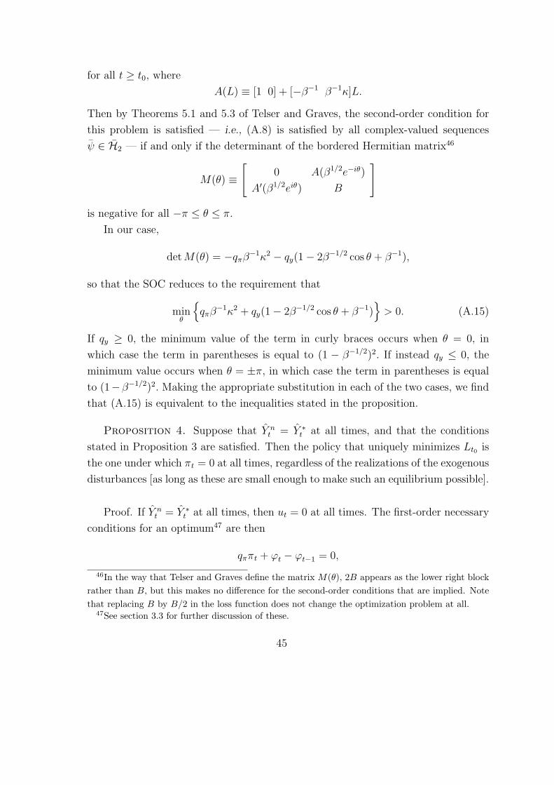
for all t ≥ t0, where

A(L) ≡ [1 0] + [−β−1 β−1κ]L.

Then by Theorems 5.1 and 5.3 of Telser and Graves, the second-order condition for

this problem is satisfied — i.e., (A.8) is satisfied by all complex-valued sequences

ψ ∈ H2 — if and only if the determinant of the bordered Hermitian matrix46

M(θ) ≡[

0 A(β1/2e−iθ)

A′(β1/2eiθ) B

]

is negative for all −π ≤ θ ≤ π.

In our case,

det M(θ) = −qπβ−1κ2 − qy(1− 2β−1/2 cos θ + β−1),

so that the SOC reduces to the requirement that

minθ

qπβ−1κ2 + qy(1− 2β−1/2 cos θ + β−1)

> 0. (A.15)

If qy ≥ 0, the minimum value of the term in curly braces occurs when θ = 0, in

which case the term in parentheses is equal to (1 − β−1/2)2. If instead qy ≤ 0, the

minimum value occurs when θ = ±π, in which case the term in parentheses is equal

to (1−β−1/2)2. Making the appropriate substitution in each of the two cases, we find

that (A.15) is equivalent to the inequalities stated in the proposition.

Proposition 4. Suppose that Y nt = Y ∗

t at all times, and that the conditions

stated in Proposition 3 are satisfied. Then the policy that uniquely minimizes Lt0 is

the one under which πt = 0 at all times, regardless of the realizations of the exogenous

disturbances [as long as these are small enough to make such an equilibrium possible].

Proof. If Y nt = Y ∗

t at all times, then ut = 0 at all times. The first-order necessary

conditions for an optimum47 are then

qππt + ϕt − ϕt−1 = 0,

46In the way that Telser and Graves define the matrix M(θ), 2B appears as the lower right blockrather than B, but this makes no difference for the second-order conditions that are implied. Notethat replacing B by B/2 in the loss function does not change the optimization problem at all.

47See section 3.3 for further discussion of these.

45

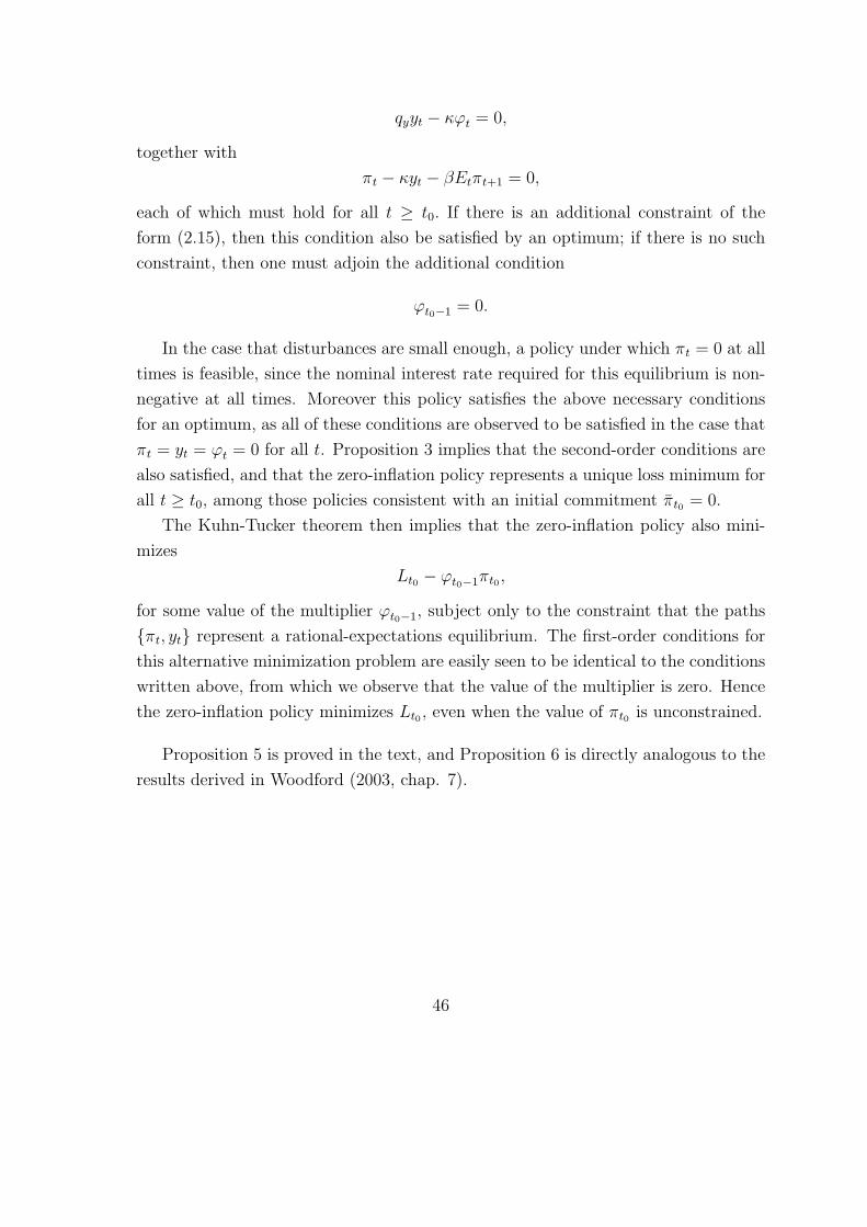
qyyt − κϕt = 0,

together with

πt − κyt − βEtπt+1 = 0,

each of which must hold for all t ≥ t0. If there is an additional constraint of the

form (2.15), then this condition also be satisfied by an optimum; if there is no such

constraint, then one must adjoin the additional condition

ϕt0−1 = 0.

In the case that disturbances are small enough, a policy under which πt = 0 at all

times is feasible, since the nominal interest rate required for this equilibrium is non-

negative at all times. Moreover this policy satisfies the above necessary conditions

for an optimum, as all of these conditions are observed to be satisfied in the case that

πt = yt = ϕt = 0 for all t. Proposition 3 implies that the second-order conditions are

also satisfied, and that the zero-inflation policy represents a unique loss minimum for

all t ≥ t0, among those policies consistent with an initial commitment πt0 = 0.

The Kuhn-Tucker theorem then implies that the zero-inflation policy also mini-

mizes

Lt0 − ϕt0−1πt0 ,

for some value of the multiplier ϕt0−1, subject only to the constraint that the paths

πt, yt represent a rational-expectations equilibrium. The first-order conditions for

this alternative minimization problem are easily seen to be identical to the conditions

written above, from which we observe that the value of the multiplier is zero. Hence

the zero-inflation policy minimizes Lt0 , even when the value of πt0 is unconstrained.

Proposition 5 is proved in the text, and Proposition 6 is directly analogous to the

results derived in Woodford (2003, chap. 7).

46

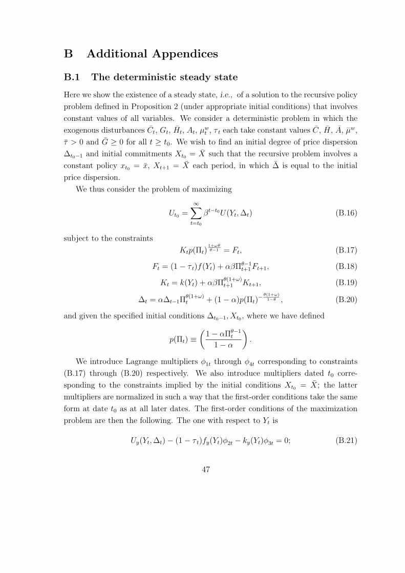
B Additional Appendices

B.1 The deterministic steady state

Here we show the existence of a steady state, i.e., of a solution to the recursive policy

problem defined in Proposition 2 (under appropriate initial conditions) that involves

constant values of all variables. We consider a deterministic problem in which the

exogenous disturbances Ct, Gt, Ht, At, µwt , τ t each take constant values C, H, A, µw,

τ > 0 and G ≥ 0 for all t ≥ t0. We wish to find an initial degree of price dispersion

∆t0−1 and initial commitments Xt0 = X such that the recursive problem involves a

constant policy xt0 = x, Xt+1 = X each period, in which ∆ is equal to the initial

price dispersion.

We thus consider the problem of maximizing

Ut0 =∞∑

t=t0

βt−t0U(Yt, ∆t) (B.16)

subject to the constraints

Ktp(Πt)1+ωθθ−1 = Ft, (B.17)

Ft = (1− τ t)f(Yt) + αβΠθ−1t+1Ft+1, (B.18)

Kt = k(Yt) + αβΠθ(1+ω)t+1 Kt+1, (B.19)

∆t = α∆t−1Πθ(1+ω)t + (1− α)p(Πt)

− θ(1+ω)1−θ , (B.20)

and given the specified initial conditions ∆t0−1, Xt0 , where we have defined

p(Πt) ≡(

1− αΠθ−1t

1− α

).

We introduce Lagrange multipliers φ1t through φ4t corresponding to constraints

(B.17) through (B.20) respectively. We also introduce multipliers dated t0 corre-

sponding to the constraints implied by the initial conditions Xt0 = X; the latter

multipliers are normalized in such a way that the first-order conditions take the same

form at date t0 as at all later dates. The first-order conditions of the maximization

problem are then the following. The one with respect to Yt is

Uy(Yt, ∆t)− (1− τ t)fy(Yt)φ2t − ky(Yt)φ3t = 0; (B.21)

47

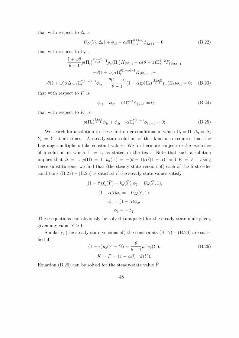
that with respect to ∆t is

U∆(Yt, ∆t) + φ4t − αβΠθ(1+ω)t+1 φ4,t+1 = 0; (B.22)

that with respect to Πtis

1 + ωθ

θ − 1p(Πt)

(1+ωθ)θ−1

−1pπ(Πt)Ktφ1,t − α(θ − 1)Πθ−2t Ftφ2,t−1

−θ(1 + ω)αΠθ(1+ω)−1t Ktφ3,t−1+

−θ(1 + ω)α∆t−1Πθ(1+ω)−1t φ4t −

θ(1 + ω)

θ − 1(1− α)p(Πt)

(1+ωθ)θ−1 pπ(Πt)φ4t = 0; (B.23)

that with respect to Ft is

−φ1t + φ2t − αΠθ−1t φ2,t−1 = 0; (B.24)

that with respect to Kt is

p(Πt)1+ωθθ−1 φ1t + φ3t − αΠ

θ(1+ω)t φ3,t−1 = 0; (B.25)

We search for a solution to these first-order conditions in which Πt = Π, ∆t = ∆,

Yt = Y at all times. A steady-state solution of this kind also requires that the

Lagrange multipliers take constant values. We furthermore conjecture the existence

of a solution in which Π = 1, as stated in the text. Note that such a solution

implies that ∆ = 1, p(Π) = 1, pπ(Π) = −(θ − 1)α/(1 − α), and K = F . Using

these substitutions, we find that (the steady-state version of) each of the first-order

conditions (B.21) – (B.25) is satisfied if the steady-state values satisfy

[(1− τ)fy(Y )− ky(Y )]φ2 = Uy(Y , 1),

(1− αβ)φ4 = −U∆(Y , 1),

φ1 = (1− α)φ2,

φ3 = −φ2.

These equations can obviously be solved (uniquely) for the steady-state multipliers,

given any value Y > 0.

Similarly, (the steady-state versions of) the constraints (B.17) – (B.20) are satis-

fied if

(1− τ)uc(Y − G) =θ

θ − 1µwvy(Y ), (B.26)

K = F = (1− αβ)−1k(Y ),

Equation (B.26) can be solved for the steady-state value Y .

48

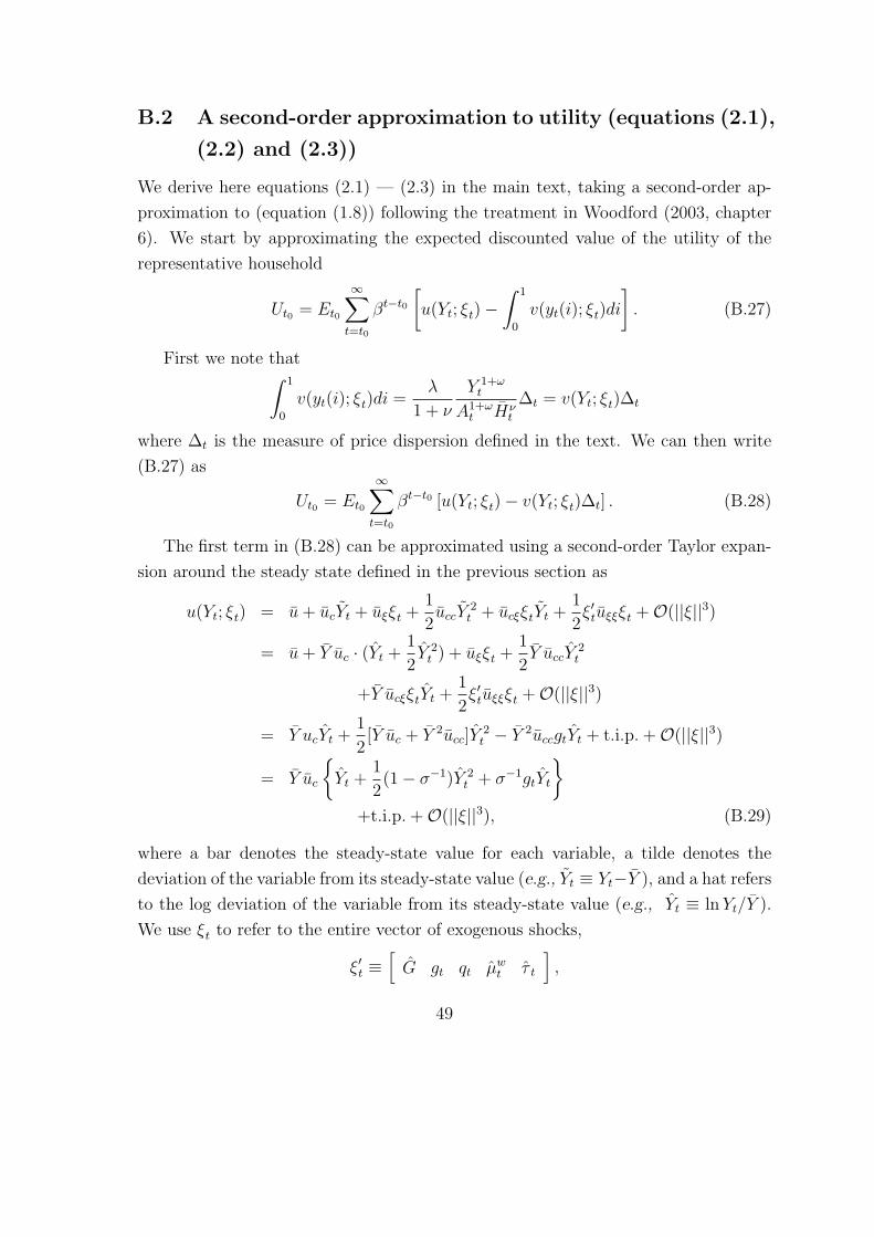
B.2 A second-order approximation to utility (equations (2.1),

(2.2) and (2.3))

We derive here equations (2.1) — (2.3) in the main text, taking a second-order ap-

proximation to (equation (1.8)) following the treatment in Woodford (2003, chapter

6). We start by approximating the expected discounted value of the utility of the

representative household

Ut0 = Et0

∞∑t=t0

βt−t0

[u(Yt; ξt)−

∫ 1

0

v(yt(i); ξt)di

]. (B.27)

First we note that∫ 1

0

v(yt(i); ξt)di =λ

1 + ν

Y 1+ωt

A1+ωt Hν

t

∆t = v(Yt; ξt)∆t

where ∆t is the measure of price dispersion defined in the text. We can then write

(B.27) as

Ut0 = Et0

∞∑t=t0

βt−t0 [u(Yt; ξt)− v(Yt; ξt)∆t] . (B.28)

The first term in (B.28) can be approximated using a second-order Taylor expan-

sion around the steady state defined in the previous section as

u(Yt; ξt) = u + ucYt + uξξt +1

2uccY

2t + ucξξtYt +

1

2ξ′tuξξξt +O(||ξ||3)

= u + Y uc · (Yt +1

2Y 2

t ) + uξξt +1

2Y uccY

2t

+Y ucξξtYt +1

2ξ′tuξξξt +O(||ξ||3)

= Y ucYt +1

2[Y uc + Y 2ucc]Y

2t − Y 2uccgtYt + t.i.p. +O(||ξ||3)

= Y uc

Yt +

1

2(1− σ−1)Y 2

t + σ−1gtYt

+t.i.p. +O(||ξ||3), (B.29)

where a bar denotes the steady-state value for each variable, a tilde denotes the

deviation of the variable from its steady-state value (e.g., Yt ≡ Yt−Y ), and a hat refers

to the log deviation of the variable from its steady-state value (e.g., Yt ≡ ln Yt/Y ).

We use ξt to refer to the entire vector of exogenous shocks,

ξ′t ≡[

G gt qt µwt τ t

],

49

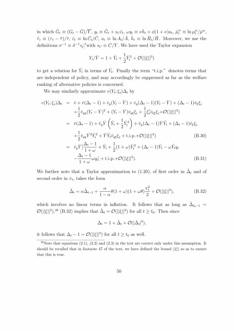
in which Gt ≡ (Gt − G)/Y , gt ≡ Gt + sC ct, ωqt ≡ νht + φ(1 + ν)at, µwt ≡ ln µw

t /µw,

τ t ≡ (τ t − τ)/τ , ct ≡ ln Ct/C, at ≡ ln At/A, ht ≡ ln Ht/H. Moreover, we use the

definitions σ−1 ≡ σ−1s−1C with sC ≡ C/Y . We have used the Taylor expansion

Yt/Y = 1 + Yt +1

2Y 2

t +O(||ξ||3)

to get a relation for Yt in terms of Yt. Finally the term “t.i.p.” denotes terms that

are independent of policy, and may accordingly be suppressed as far as the welfare

ranking of alternative policies is concerned.

We may similarly approximate v(Yt; ξt)∆t by

v(Yt; ξt)∆t = v + v(∆t − 1) + vy(Yt − Y ) + vy(∆t − 1)(Yt − Y ) + (∆t − 1)vξξt

+1

2vyy(Yt − Y )2 + (Yt − Y )vyξξt +

1

2ξ′tvξξξt+O(||ξ||3)

= v(∆t − 1) + vyY

(Yt +

1

2Y 2

t

)+ vy(∆t − 1)Y Yt + (∆t − 1)vξξt

+1

2vyyY

2Y 2t + Y Ytvyξξt + t.i.p.+O(||ξ||3) (B.30)

= vyY [∆t − 1

1 + ω+ Yt +

1

2(1 + ω)Y 2

t + (∆t − 1)Yt − ωYtqt

−∆t − 1

1 + ωωqt] + t.i.p.+O(||ξ||3). (B.31)

We further note that a Taylor approximation to (1.20), of first order in ∆t and of

second order in πt, takes the form

∆t = α∆t−1 +α

1− αθ(1 + ω)(1 + ωθ)

π2t

2+O(||ξ||3), (B.32)

which involves no linear terms in inflation. It follows that as long as ∆t0−1 =

O(||ξ||2),48 (B.32) implies that ∆t = O(||ξ||2) for all t ≥ t0. Then since

∆t = 1 + ∆t +O(|∆t|2),

it follows that ∆t − 1 = O(||ξ||2) for all t ≥ t0 as well.

48Note that equations (2.1), (2.2) and (2.3) in the text are correct only under this assumption. Itshould be recalled that in footnote 47 of the text, we have defined the bound ||ξ|| so as to ensurethat this is true.

50

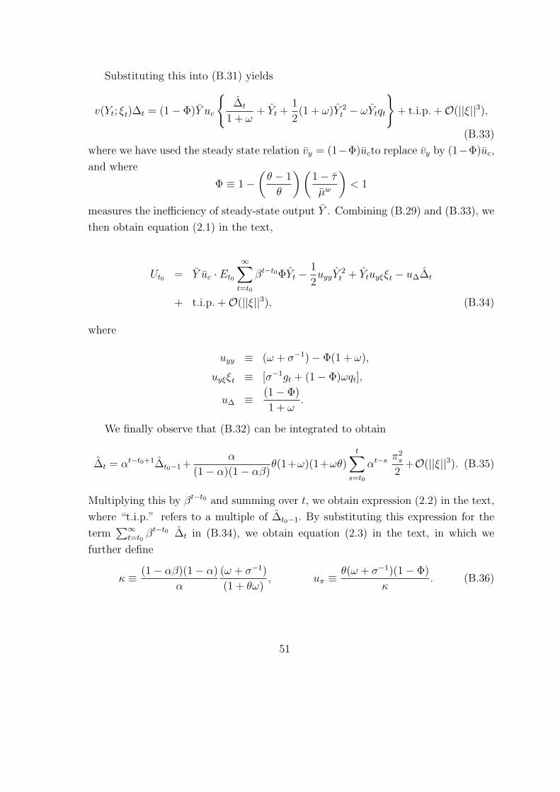
Substituting this into (B.31) yields

v(Yt; ξt)∆t = (1− Φ)Y uc

∆t

1 + ω+ Yt +

1

2(1 + ω)Y 2

t − ωYtqt

+ t.i.p. +O(||ξ||3),

(B.33)

where we have used the steady state relation vy = (1−Φ)ucto replace vy by (1−Φ)uc,

and where

Φ ≡ 1−(

θ − 1

θ

)(1− τ

µw

)< 1

measures the inefficiency of steady-state output Y . Combining (B.29) and (B.33), we

then obtain equation (2.1) in the text,

Ut0 = Y uc · Et0

∞∑t=t0

βt−t0ΦYt − 1

2uyyY

2t + Ytuyξξt − u∆∆t

+ t.i.p. +O(||ξ||3), (B.34)

where

uyy ≡ (ω + σ−1)− Φ(1 + ω),

uyξξt ≡ [σ−1gt + (1− Φ)ωqt],

u∆ ≡ (1− Φ)

1 + ω.

We finally observe that (B.32) can be integrated to obtain

∆t = αt−t0+1∆t0−1 +α

(1− α)(1− αβ)θ(1+ω)(1+ωθ)

t∑s=t0

αt−s π2s

2+O(||ξ||3). (B.35)

Multiplying this by βt−t0 and summing over t, we obtain expression (2.2) in the text,

where “t.i.p.” refers to a multiple of ∆t0−1. By substituting this expression for the

term∑∞

t=t0βt−t0 ∆t in (B.34), we obtain equation (2.3) in the text, in which we

further define

κ ≡ (1− αβ)(1− α)

α

(ω + σ−1)

(1 + θω), uπ ≡ θ(ω + σ−1)(1− Φ)

κ. (B.36)

51

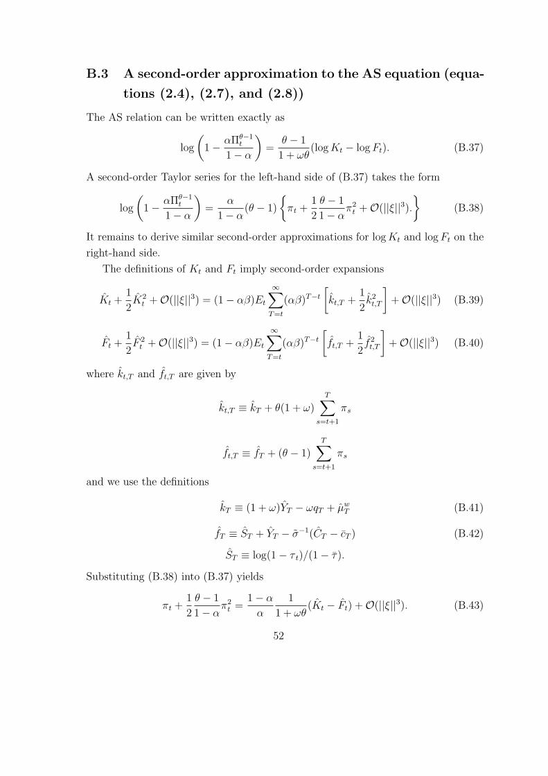
B.3 A second-order approximation to the AS equation (equa-

tions (2.4), (2.7), and (2.8))

The AS relation can be written exactly as

log

(1− αΠθ−1

t

1− α

)=

θ − 1

1 + ωθ(log Kt − log Ft). (B.37)

A second-order Taylor series for the left-hand side of (B.37) takes the form

log

(1− αΠθ−1

t

1− α

)=

α

1− α(θ − 1)

πt +

1

2

θ − 1

1− απ2

t +O(||ξ||3).

(B.38)

It remains to derive similar second-order approximations for log Kt and log Ft on the

right-hand side.

The definitions of Kt and Ft imply second-order expansions

Kt +1

2K2

t +O(||ξ||3) = (1− αβ)Et

∞∑T=t

(αβ)T−t

[kt,T +

1

2k2

t,T

]+O(||ξ||3) (B.39)

Ft +1

2F 2

t +O(||ξ||3) = (1− αβ)Et

∞∑T=t

(αβ)T−t

[ft,T +

1

2f 2

t,T

]+O(||ξ||3) (B.40)

where kt,T and ft,T are given by

kt,T ≡ kT + θ(1 + ω)T∑

s=t+1

πs

ft,T ≡ fT + (θ − 1)T∑

s=t+1

πs

and we use the definitions

kT ≡ (1 + ω)YT − ωqT + µwT (B.41)

fT ≡ ST + YT − σ−1(CT − cT ) (B.42)

ST ≡ log(1− τ t)/(1− τ).

Substituting (B.38) into (B.37) yields

πt +1

2

θ − 1

1− απ2

t =1− α

α

1

1 + ωθ(Kt − Ft) +O(||ξ||3). (B.43)

52

Note that to first order, this reduces to

πt =1− α

α

1

1 + ωθ(Kt − Ft) +O(||ξ||2) (B.44)

=(1− α)(1− αβ)

α

1

1 + ωθEt

∞∑T=t

(αβ)T−t[kt,T − ft,T

]+O(||ξ||2). (B.45)

We can use (B.39)–(B.40) to obtain a second-order expansion for the right-hand

side of (B.43). Subtracting (B.40) from (B.39), we obtain

Kt − Ft = (1− αβ)Et

∞∑T=t

(αβ)T−t

[(kt,T − ft,T ) +

1

2(k2

t,T − f 2t,T )

]

−1

2(K2

t − F 2t ) +O(||ξ||3)

= (1− αβ)Et

∞∑T=t

(αβ)T−t

[(kt,T − ft,T ) +

1

2(k2

t,T − f 2t,T )

](B.46)

−1

2(Kt − Ft)(Kt + Ft) +O(||ξ||3)

= (1− αβ)Et

∞∑T=t

(αβ)T−t

[(kt,T − ft,T ) +

1

2(k2

t,T − f 2t,T )

](B.47)

−1

2(1− αβ)

α

(1− α)(1 + ωθ)πtZt +O(||ξ||3),

where in passing from (B.46) to (B.47) we have used (B.44) to substitute for (Kt−Ft)

in the second term on the right-hand side, and

(Kt + Ft) = (1− αβ)Zt +O(||ξ||2)

to substitute for (Kt + Ft), in which expression we define

Zt ≡ Et

∞∑T=t

(αβ)T−t[kt,T + ft,T

]. (B.48)

We can use the definitions of kt,T and ft,T to further expand the first term on the

right-hand side of (B.47). We obtain

Et

∞∑T=t

(αβ)T−t[kt,T − ft,T

]= Et

∞∑T=t

(αβ)T−t[kT − fT

]+ (1 + ωθ)Et

∞∑T=t

(αβ)T−t

T∑s=t+1

πs

= Et

∞∑T=t

(αβ)T−t[kT − fT

]+

(1 + ωθ)

1− αβPt, (B.49)

53

where

Pt ≡ Et

∞∑T=t+1

(αβ)T−tπT , (B.50)

and

1

2Et

∞∑T=t

(αβ)T−t[k2

t,T − f 2t,T

]=

1

2Et

∞∑T=t

(αβ)T−t[k2

T − f 2T

]

+Et

∞∑T=t

(αβ)T−t[θ(1 + ω)kT + (1− θ)fT ] ·T∑

s=t+1

πs

+1

2(2θ + θω − 1)(1 + θω)Et

∞∑T=t

(αβ)T−t

(T∑

s=t+1

πs

)2

=1

2Et

∞∑T=t

(αβ)T−t[k2

T − f 2T

]+ Et

∞∑T=t+1

(αβ)T−tπT NT

+1

2

(2θ + θω − 1)(1 + θω)

(1− αβ)Et

∞∑T=t+1

(αβ)T−tπT (πT + 2PT )

where

Nt ≡ Et

∞∑T=t

(αβ)T−t[θ(1 + ω)kT + (1− θ)fT ]. (B.51)

Substituting these expressions into (B.47), we obtain

Kt − Ft = (1− αβ)Et

∞∑T=t

(αβ)T−t

[(kT − fT ) +

1

2(k2

T − f 2T )

]+

+(1 + ωθ)Et

∞∑T=t+1

(αβ)T−tπT + (1− αβ)Et

∞∑T=t+1

(αβ)T−tπT NT +

1

2(2θ + θω − 1)(1 + θω)Et

∞∑T=t+1

(αβ)T−tπT (πT + 2PT )

−1

2(1− αβ)

α

(1− α)(1 + ωθ)πtZt +O(||ξ||3). (B.52)

54

This can be written recursively as

Kt − Ft +1

2

α(1− αβ)(1 + ωθ)

(1− α)πtZt = (1− αβ)

[(kt − ft) +

1

2(k2

t − f 2t )

]+

+αβ(1 + ωθ)Etπt+1 + (1− αβ)αβEtπt+1Nt+1 +1

2(2θ + θω − 1)(1 + θω)Etπt+1(πt+1 + 2Pt+1) +

+αβEt

[Kt+1 − Ft+1 +

1

2

α(1− αβ)(1 + ωθ)

(1− α)πt+1Zt+1

]+

+O(||ξ||3) (B.53)

Using (B.43) to substitute for Kt − Ft in (B.53), we obtain

πt +1

2

θ − 1

1− απ2

t +1

2(1− αβ)πtZt =

1− α

α

(1− αβ)

(1 + ωθ)

[(kt − ft) +

1

2(k2

t − f 2t )

]+

+(1− α)βEtπt+1 + (1− α)β(1− αβ)

(1 + θω)Etπt+1Nt+1 +

1

2(2θ + θω − 1)(1− α)βEtπt+1(πt+1 + 2Pt+1) +

+αβEt

[πt+1 +

1

2

θ − 1

1− απ2

t+1 +1

2(1− αβ)πt+1Zt+1

]+

+O(||ξ||3). (B.54)

This is our second-order approximation to the AS relation. Note that to first order,

this reduces to

πt =1− α

α

(1− αβ)

(1 + ωθ)(kt − ft) + βEtπt+1 +O(||ξ||2), (B.55)

as could also have been obtained directly from (B.45).

We can furthermore eliminate Nt by observing that (B.51) implies that

Nt ≡ 1

2Et

∞∑T=t

(αβ)T−t[(1 + θω)(kt + ft) + (2θ + θω − 1)(kt − ft)]

=1

2Et

∞∑T=t

(αβ)T−t[(1 + θω)(kt,T + ft,T ) + (2θ + θω − 1)(kt,T − ft,T )]

−(2θ + θω − 1)(1 + θω)

(1− αβ)Pt

=1

2(1 + θω)Zt +

1

2(2θ + θω − 1)

(1 + θω)

1− α

α

(1− αβ)πt

−(2θ + θω − 1)(1 + θω)

(1− αβ)Pt (B.56)

55

By substituting (B.56) into (B.54), we obtain

πt +1

2

θ − 1

1− απ2

t +1

2(1− αβ)πtZt =

1− α

α

(1− αβ)

(1 + ωθ)

[(kt − ft) +

1

2(k2

t − f 2t )

]+

+βEtπt+1 +1

2β(1− αβ)Etπt+1Zt+1 +

1

2(2θ + θω − 1)βEtπ

2t+1 + αβEt

[1

2

θ − 1

1− απ2

t+1

]+

+O(||ξ||3),

which can be rewritten as

πt +1

2

θ − 1

1− απ2

t +1

2(1− αβ)πtZt =

1− α

α

(1− αβ)

(1 + ωθ)

[(kt − ft) +

1

2(k2

t − f 2t )

]

+βEtπt+1 +1

2β(1− αβ)Etπt+1Zt+1 + βEt

[1

2

θ − 1

1− απ2

t+1

]

+1

2θ(1 + ω)βEtπ

2t+1 +O(||ξ||3). (B.57)

This is a relation of the form (2.4); it can be integrated forward to obtain a relation

of the form (2.8),

Vt0 =1− α

α

(1− αβ)

(1 + ωθ)Et

∞∑t=t0

(αβ)t−t0

[(kt − ft) +

1

2(k2

t − f 2t )

]+

1

2θ(1+ω)Et

∞∑t=t0

(αβ)t−t0π2t ,

(B.58)

where

Vt ≡ πt − 1

2

1− θ

1− απ2

t +1

2(1− αβ)πtZt +

1

2θ(1 + ω)π2

t . (B.59)

Note that this last definition is of the form (2.5) given in the text, where the coeffi-

cients are defined as

vπ ≡ θ(1 + ω)− 1− θ

(1− α), vz ≡ (1− αβ)

2.

We then obtain the relations given in the text by substituting into the above

equations the definitions (B.41) for kt and (B.42) for ft. In the expression for ft, we

can furthermore use a second-order approximation to the identity Yt = Ct + Gt to

solve for Ct as a function of Yt and exogenous disturbances,

Ct = s−1C Yt − s−1

C Gt +s−1

C (1− s−1C )

2Y 2

t + s−2C YtGt + s.o.t.i.p. +O(||ξ||3), (B.60)

56

where “s.o.t.i.p” refers to second-order (or higher) terms independent of policy; the

first-order terms have been kept as these will matter for the log-linear aggregate-

supply relation that appears as a constraint in our policy problem. We similarly note

that

St = −ωτ τ t + s.o.t.i.p. +O(||ξ||3), (B.61)

where ωτ ≡ τ /(1 − τ). Equations (B.60) – (B.61) can be used to substitute for Ct

and St in (B.42), resulting in an expression for ft that involves only Yt and elements

of ξt.

Substituting these expressions for kt and ft into (B.57), we obtain equation (2.4)

in the text, where we define

cξξt ≡ (ω + σ−1)−1[−σ−1gt − ωqt + µwt + ωτ τ t],

cyy ≡ (2 + ω − σ−1) + σ−1(1− s−1C )(ω + σ−1)−1,

cyξξt ≡ (ω + σ−1)−1[−σ−1s−1C Gt + σ−1(1− σ−1)gt + ω(1 + ω)qt

−(1 + ω)µwt − (1− σ−1)ωτ τ t],

cπ ≡ θ(1 + ω)

κ,

and κ is again the coefficient defined in (B.36). (Note that κ > 0, as asserted in

the text.) The same substitutions into definition (B.48) allow us to define Zt by an

expression of the form (2.6) given in the text, where

zy ≡ (2 + ω − σ−1) + vk(ω + σ−1),

zξξt ≡ σ−1(1− vk)gt − ω(1 + vk)qt + (1 + vk)µwt − ωτ (1− vk)τ t,

zπ ≡ −(ω + σ−1)

κvk,

in which expressions we define

vk ≡ κ

(ω + σ−1)

α

1− αβ(1− 2θ − ωθ).

To a first-order approximation, equation (2.4) reduces to equation (2.7) given in

the text. Finally, the same substitutions for kt and ft into (B.58) yields equation

57

(2.8) in the text, where the term cξξt is now included in terms independent of policy.

(Such terms matter when part of the log-linear constraints, as in the case of (2.7),

but not when part of the quadratic objective.)

B.4 Derivation of equation (2.9)

We can multiply equation (2.8) by ΦY uc and subtract from (2.1) to obtain

Ut0 = −Y ucEt0

∞∑t=t0

βt−t0

1

2qyY

2t − Yt(uyξξt + Φcyξξt) +

1

2qππ2

t

+Tt0+t.i.p.+O(||ξ||3),

where

qπ ≡ uπ + Φcπ

=θ(ω + σ−1)(1− Φ)

κ+ Φ

θ(1 + ω)

κ

=θ

κ[(ω + σ−1) + Φ(1− σ−1)],

qy ≡ uyy + Φcyy

= (ω + σ−1)− Φ(1 + ω) + Φ(2 + ω − σ−1) + Φσ−1(1− s−1C )(ω + σ−1)−1

= (ω + σ−1) + Φ(1− σ−1) +Φσ−1(1− s−1

C )

ω + σ−1.

This can be rewritten in the form (2.9) given in the text, where

Y ∗t ≡ q−1

y [uyξξt + Φcyξξt]

= q−1y σ−1gt + (1− Φ)ωqt + (ω + σ−1)−1Φ[−σ−1s−1

C Gt + σ−1(1− σ−1)gt + ω(1 + ω)qt

−(1 + ω)µwt − (1− σ−1)ωτ τ t]

= ω1Ynt − ω2Gt + ω3u

wt + ω4τ t,

and Ω, Y nt , and the ωi are defined as in the text.

58

References

[1] Benigno, Gianluca, and Pierpaolo Benigno (2004), “Designing Targeting Rules

for International Monetary Policy Cooperation,” unpublished, London School of

Economics, August.

[2] Benigno, Pierpaolo, and Michael Woodford (2003), “Optimal Monetary and Fis-

cal Policy: A Linear-Quadratic Approach,” in M. Gertler and K. Rogoff, eds.,

NBER Macroeconomics Annual 2003, vol. 18, forthcoming.

[3] Benigno, Pierpaolo, and Michael Woodford (2004a), “Inflation Stabilization and

Welfare: The Case of a Distorted Steady State,” presented at the CEPR Euro-

pean Summer Symposium in Macroeconomics, Tarragona, May.

[4] Benigno, Pierpaolo, and Michael Woodford (2004b), “Optimal Stabilization Pol-

icy when Wages and Prices are Sticky: The Case of a Distorted Steady State,”

unpublished, New York University, July.

[5] Benigno, Pierpaolo, and Michael Woodford (2004c), “Optimal Policy under Re-

cursive Commitment: A Linear-Quadratic Approach ,” in preparation.

[6] Calvo, Guillermo (1983), “Staggered Prices in a Utility-Maximizing Framework,”

Journal of Monetary Economics, 12: 383-398.

[7] Chari, V.V., Patrick J. Kehoe, and Ellen R. McGrattan, “Sticky Price Models of

the Business Cycle: Can the Contract Multiplier Solve the Persistence Problem?”

Econometrica 68: 1151-1179 (2000).

[8] Clarida, Richard, Jordi Gali, and Mark Gertler (1999), “The Science of Monetary

Policy: a New Keynesian Perspective,” Journal of Economic Literature, 37 (4),

pp. 1661-1707.

[9] Dupor, William (2003), “Optimal Random Monetary Policy with Nominal Rigid-

ity,” Journal of Economic Theory, 112 (1): 66-78.

[10] Erceg, Christopher J., Dale W. Henderson, and Andrew T. Levin, “Optimal

Monetary Policy with Staggered Wage and Price Contracts,” Journal of Mone-

tary Economics 46: 281-313 (2000).

59

[11] Giannoni, Marc, and Michael Woodford (2002), “Optimal Interest-Rate Rules:

I. General Theory,”NBER working paper no. 9419, December.

[12] Giannoni, Marc, and Michael Woodford (2003), “Optimal Inflation Targeting

Rules,”in B.S. Bernanke and M. Woodford, eds., The Inflation Targeting Debate,

Chicago: University of Chicago Press, forthcoming.

[13] Goodfriend, Marvin, and Robert King (1997), “The New Neoclassical Synthesis

and the Role of Monetary Policy,” in B.S. Bernanke and J.J. Rotemberg (eds.),

NBER Macroeconomic Annual 1997, Cambridge, MA: MIT press.

[14] Khan, Aubhik, Robert G. King, and Alexander L. Wolman (2003), “Optimal

Monetary Policy,” Review of Economic Studies 70(4): 825-860.

[15] Kim, Jinill, Sunghyun Kim, Ernst Schaumburg, and Christopher A. Sims (2003),

“Calculating and Using Second Order Accurate Solutions of Discrete Time Dy-

namic Equilibrium Models ,” unpublished manuscript, University of Virginia,

June.

[16] King, Robert G., and Alexander L. Wolman (1999), “What Should the Monetary

Authority Do when Prices are Sticky,” in J.B. Taylor, ed., Monetary Policy Rules,

Chicago: University of Chicago Press.

[17] Rotemberg, Julio J., and Michael Woodford (1997), “An Optimization-Based

Econometric Framework for the Evaluation of Monetary Policy”, in B.S.

Bernanke and Rotemberg (eds.), NBER Macroeconomic Annual 1997, Cam-

bridge, MA: MIT Press. 297-346.

[18] Sutherland, Alan (2002), “A Simple Second-Order Solution Method for Dynamic

General Equilibrium Models,” unpublished manuscript, University of St. An-

drews.

[19] Telser, Lester G., and Robert L. Graves (1972), Functional Analysis in Mathe-

matical Economics: Optimization over Infinite Horizons, Chicago: University of

Chicago Press.

[20] Walsh, Carl (2003), Monetary Theory and Policy, 2nd edition, Cambridge,

MA:MIT Press.

60

[21] Woodford, Michael (1999), “Commentary: How Should Monetary Policy Be

Conducted in an Era of Price Stability?”in Federal Reserve Bank of Kansas

City, New Challenges for Monetary Policy.

[22] Woodford, Michael (2001), “Fiscal Requirements for Price Stability,”Journal of

Money, Credit and Banking 33: 669-728.

[23] Woodford, Michael (2003), Interest and Prices: Foundations of a Theory of

Monetary Policy, Princeton University Press.

61