inflation implications of rising government debt … · inflation implications of rising government...
TRANSCRIPT

NBER WORKING PAPER SERIES
INFLATION IMPLICATIONS OF RISING GOVERNMENT DEBT
Chryssi GiannitsarouAndrew Scott
Working Paper 12654http://www.nber.org/papers/w12654
NATIONAL BUREAU OF ECONOMIC RESEARCH1050 Massachusetts Avenue
Cambridge, MA 02138October 2006
We thank Boris Glass for extensive research assistance and support. We are also grateful to participantsat ISOM 2006 and EEA-ESEM 2006. We are particularly grateful to Domenico Giannone, Eric Leeperand Lucrezia Reichlin for their comments and suggestions for improving this paper. The views expressedherein are those of the author(s) and do not necessarily reflect the views of the National Bureau ofEconomic Research.
© 2006 by Chryssi Giannitsarou and Andrew Scott. All rights reserved. Short sections of text, notto exceed two paragraphs, may be quoted without explicit permission provided that full credit, including© notice, is given to the source.

Inflation Implications of Rising Government DebtChryssi Giannitsarou and Andrew ScottNBER Working Paper No. 12654October 2006JEL No. E31,E62
ABSTRACT
The intertemporal budget constraint of the government implies a relationship between a ratio of currentliabilities to the primary deficit with future values of inflation, interest rates, GDP and narrow moneygrowth and changes in the primary deficit. This relationship defines a natural measure of fiscal balanceand can be used as an accounting identity to examine the channels through which governments achievefiscal sustainability. We evaluate the ability of this framework to account for the fiscal behaviour ofsix industrialised nations since 1960. We show how fiscal imbalances are mainly removed throughadjustments in the primary deficit (80-100%), with less substantial roles being played by inflation(0-10%) and GDP growth (0-20%). Focusing on the relation between fiscal imbalances and inflationsuggests extremely modest interactions. This post WWII evidence suggests that the widely anticipatedfuture increases in fiscal deficits, need not necessarily have a substantial impact on inflation.
Chryssi GiannitsarouFaculty of EconomicsUniversity of CambridgeAustin Robinson BuildingSidgwick AvenueCambridge CB3 9DD, [email protected]
Andrew ScottDepartment of EconomicsLondon Business SchoolSussex Place,London NW1 4SA, [email protected]

INFLATION IMPLICATIONS OF RISING GOVERNMENT DEBT�
C. Giannitsarouy A. Scottz
October 21, 2006
Abstract. The intertemporal budget constraint of the government implies a relationship
between a ratio of current liabilities to the primary de�cit with future values of in�ation, interest
rates, GDP and narrow money growth and changes in the primary de�cit. This relationship de�nes a
natural measure of �scal balance and can be used as an accounting identity to examine the channels
through which governments achieve �scal sustainability. We evaluate the ability of this framework to
account for the �scal behaviour of six industrialised nations since 1960. We show how �scal imbalances
are mainly removed through adjustments in the primary de�cit (80-100%), with less substantial roles
being played by in�ation (0-10%) and GDP growth (0-20%). Focusing on the relation between �scal
imbalances and in�ation suggests extremely modest interactions. This post WWII evidence suggests
that the widely anticipated future increases in �scal de�cits, need not necessarily have a substantial
impact on in�ation.
JEL classification: E31, E62
Keywords: Fiscal de�cit, �scal sustainability, government debt, in�ation, intertemporal budget
constraint.
1. Introduction
Figures 1 and 2 show recent �scal trends for six large industrialised nations. Levels of government
debt increased markedly during the 1970s, then stabilised and improved during the 1980s and 1990s,
but have recently shown signs of further deterioration. With OECD countries experiencing an ageing
population, it is widely expected that �scal positions will worsen yet further in coming decades (see
inter alia Roseveare, Leibfritz, Fore and Wurzel, 1998, for projections). These considerations raise three
important issues: (a) Is current �scal policy sustainable? (b) How have OECD governments achieved
�scal sustainability in past decades? (c) What are the implications for in�ation of these projected rising
�scal de�cits? This paper seeks to provide insights to each of these three questions.
Key to our analysis is the intertemporal budget constraint of the government. To answer the �rst
question (on sustainability), we use the methodology of Giannitsarou and Scott (2006) and derive a log
linear approximation to the intertemporal budget constraint. Using this framework, we show how debt
sustainability requires an equilibrium relationship between the market value of government debt, the
stock of narrow money and the levels of government revenue and expenditure. We show how to estimate
�We thank Boris Glass for extensive research assistance and support. We are also grateful to seminar participants atISOM 2006, and EEA 2006 Vienna. We would like to thank in particular Domenico Giannone, Eric Leeper and LucreziaReichlin for their comments and suggestions for improving this paper.
yFaculty of Economics, University of Cambridge and CEPR. E-mail: [email protected] Department, London Business School and CEPR. E-mail: [email protected].
1

Inflation and Rising Debt 2
this relationship and derive a measure of sustainability for six OECD countries and use our estimates
to characterise the dynamics of �scal adjustment for our six countries. In order to answer the second
question (how do governments achieve �scal adjustment) we show analytically how deviations from the
equilibrium relationship between debt, money and the primary de�cit have to be met through future
changes in either primary de�cits, monetary liabilities, real interest rates, in�ation or GDP growth. Using
the VAR methodology proposed by Campbell and Shiller (1988), we assess the relative contribution of
each channel to �nancing �scal activity, for the period 1960-2005. Our third and �nal focus is to use this
framework to assess statistically whether the substantial expected increase in �scal de�cits threatens the
current low levels of in�ation.
Our �ndings can be summarised as follows. For the period under consideration and for US, Japan,
Germany, UK, Italy and Canada, �scal imbalances are mostly removed through adjustments in the
primary de�cit (80-100%), with less important adjustments through in�ation (0-10%) and GDP growth
(0-20%). In particular, the relation between �scal imbalances and in�ation suggests extremely modest
statistical interactions between the two; suggesting that widely anticipated increases in �scal de�cits, due
to demographic factors, are not necessarily predictors of higher future in�ation. It is important to stress
that this conclusion is based around an analysis which is in essence a purely accounting exercise. There
exists a large and varied theoretical literature examining the economic linkages between �scal de�cits
and in�ation (see inter alia Sargent and Wallace, 1981, McCallum, 1984, Leeper, 1991, Sims, 1994 and
Woodford, 1995) but, by contrast, our analysis pursues a di¤erent path. Using the accounting framework
of the intertemporal budget constraint to empirically document the relative statistical role of di¤erent
factors in achieving �scal balance.
The plan of the paper is as follows. In Section 2 we examine the properties of our data set and
argue that our sample period is appropriate for reviewing how �scal adjustment is achieved in the
face of large variations in government debt in response to sharp increases in social transfers. Using
the period-by-period budget constraint we examine evidence for �scal sustainability and the drivers of
the debt/GDP ratio. A simple accounting exercise shows that nominal GDP growth, and especially
in�ation, played an important role in achieving debt stability. In Section 3 we extend our analysis and
introduce our log linearised version of the intertemporal budget constraint and derive our key measure of
�scal imbalances, namely a relationship between levels of government liabilities and the primary de�cit.
We show how variations in this relationship are related to expected changes in future de�cits, money
creation and changes in in�ation, real interest rates and real GDP growth. In Section 4 we show how
to estimate this long run relationship between liabilities and the de�cit and we then construct estimates
of �scal imbalances across the countries in our sample and draw conclusions about the dynamics of
�scal adjustment. Section 5 builds on this long run relationship and the restrictions imposed by the
intertemporal budget constraint to perform a variance decomposition for how �scal sustainability is
achieved. We extend our framework to assess the separate importance of government expenditure and
tax revenue in achieving �scal balance and examine the predictive role of �scal imbalances in predicting
future in�ation. A �nal section concludes.

Inflation and Rising Debt 3
2. Fiscal Sustainability: A backward looking approach
Our focus is on assessing the sustainability of �scal policy in six industrial nations - US, Japan, Germany,
UK, Italy and Canada - over the period 1960-2005. Our interest is not just to assess �scal sustainability,
but also to identify the means through which this sustainability is achieved. We choose these nations
because we are interested in the implications of demographic induced de�cits that are expected to a¤ect
these countries in the coming decades. We choose this time period because, in contrast to the majority
of the literature, we are interested in how governments achieve �scal balance in the face of rising non-war
related expenditures.
With demographic change expected to lead to increasing social transfers, this sample is a natural
environment with which to consider the likely impact of rising debt. For example, over this period,
Canada increased social transfers by 4.7% of GDP, Germany by 6.6%, Italy 7.8%, Japan 9.2%, UK 5.9%
and US 6.7%. which accounted for 104%, 57%, 51%, 49%, 88% and 146% respectively of the observed
increase in total government expenditure during this period. In other words our period is one where
increases in government expenditure were heavily linked to rises in social transfers. A further reason
for focusing on this post WWII period is that it is the most recent and most relevant: our results
in Giannitsarou and Scott (2006), using historical UK and US data, suggest that the means through
which �scal adjustment is achieved have changed signi�cantly across centuries and in particular war
induced increases in debt are �nanced through di¤erent channels than general increases in debt. We
leave undiscussed the political economy features that might explain why military expenditure is �nanced
through di¤erent means to social transfers but the implication is that focusing on modern times of peace
is critical if we are to gauge the impact of demographic induced future �scal de�cits.
For this period to be informative regarding the means whereby governments achieve �scal sustain-
ability it is important that debt and de�cits show signi�cant variation. Another reason why so many
previous researchers have focused on war related expenditure is it leads to dramatic swings in public debt
and de�cits and so is a natural period with which to examine �scal sustainability. Table 1 documents
some stylised facts for key �scal variables over our post war period.1 Debt relative to GDP shows large
volatility, with a standard deviation ranging from 0.078 to 0.381. With the exception of the US, all
countries see an increase in debt/GDP over the sample period and in two of our six cases, debt/GDP
rises above 100% GDP. This is far from being a period of tranquil public �nances or modest variation in
debt, suggesting once more its relevance as a case study for coming decades.
Performing various unit root tests (see Tables 2-5) to the market value of government debt, govern-
ment expenditure (excluding interest payments) and revenue, all expressed as a ratio to GDP, provides
further evidence of the variability of government �nances. The strong consensus that emerges from
these results is that all variables appear to be non-stationary and contain unit roots. The fact that
government expenditure/GDP and tax revenue/GDP are non-stationary over this period is testimony
to the rise of social transfers commented on in previous paragraphs. The suggestion that debt/GDP is
also non-stationary further implies that achieving �scal sustainability in this post war period has been
1A detailed description of our data and its sources is provided in appendix A.

Inflation and Rising Debt 4
a challenge. The �nding that the debt/GDP ratio is non-stationary also con�icts with the �ndings of
Giannitsarou and Scott (2006) that use longer runs of historical data. It thus seems that the sample in
this paper is one of unusual �scal problems.
The �nding that debt/GDP is non-stationary may appear to be inconsistent with �scal sustainability,
but as stressed by Bohn (2006), this is not necessarily the case. Critical for sustainability, according to
this analysis, is the existence of a feedback from the level of debt to the current primary de�cit. In other
words, when estimating a regression of
PrimarySurplust = A(L)Xt + �Debtt + �t;
where Xt denotes a set of relevant explanatory variables, it is necessary that � is positive and larger
than the interest rate paid on government debt. The �nal column in Table 1 reports estimates of � (and
associated p values) for each of our countries where Xt consisted of lagged values of the primary surplus.
Only in the cases of Japan and Germany is the debt term not signi�cant at the 5% level or less (although
including additional variables such as GDP, interest rates, etc. remedied this problem for Germany),
suggesting that most countries show evidence of �scal sustainability over our period. Interestingly, Japan
and Germany are the only countries where the maximum value for debt/GDP is observed in the �nal
observation in the sample period. We include all six countries in our estimation below, but these results
suggest some care should be taken in interpreting the Japanese and German �ndings.
To better understand the movements in the debt/GDP ratio and its relationship with other �scal
variables it is useful to consider the period-by-period budget constraint. Let 1+{t denote the growth innominal GDP and 1+ it�1 the one year holding return on nominal government bonds. Let Bt, Gt and Ttbe the ratios of nominal debt, government spending and tax revenues to nominal GDP.2 Then we have
�Bt = (Gt � Tt) +it�11 + {t
Bt�1 �{t
1 + {tBt�1: (1)
In other words, the debt to GDP ratio increases through the ratio of the primary de�cit to GDP and
interest payments on debt (using the growth adjusted real interest rate), and reduces through a nominal
growth dividend {tBt�1= (1 + {t). To investigate the role of variations in bond prices as a way of ensuringthat the intertemporal budget constraint of the government holds (the focus of Marcet and Scott, 2005a),
we evaluate (1) by considering it as the one year holding return on government bonds. In other words,
we include both coupon payments and capital gains, so that our budget constraint is speci�ed in terms
of the market value of government debt, rather than the stock of outstanding debt.
Following Bohn (2005), to gain some understanding of what drives changes in the debt/GDP ratio,
we can evaluate (1) using sample averages for our period. The results are shown in Table 6. As noted
in Table 1, Japan and Germany show the most dramatic increases in debt, with only the US and UK
showing broad debt stability. These substantial di¤erences in debt dynamics are despite the fact that,
with the exception of Italy, the total de�cit/GDP ratio is reasonably similar across countries. The main
2For easy reference, the notation we use throughout the paper is summarised in Appendix B.

Inflation and Rising Debt 5
reason behind Germany and Japan�s di¤erent debt dynamics is their low value of the growth dividend;
this is particularly noticeable for the in�ation component (the nominal growth dividend consists of a real
growth and an in�ation component). Reviewing Table 6, it is seems that in�ation has been a signi�cant
in�uence in achieving �scal sustainability. At �rst glance, this would seem to generate the serious concern
that rising de�cits induced by demographic change may lead to rising in�ation.
Table 6 is a useful accounting exercise, but in focusing on ex post realisations only provides a backward
looking analysis. Equation (1) holds for all �scal policies, regardless of whether they are sustainable or
not, and as a consequence cannot be used to assess the sustainability of �scal policy. Moreover, it does
not provide information on how governments expect to achieve �scal sustainability or how �scal policy
responds to shocks to key economic variables. In order to gain insights into these issues we next turn to
a forward looking perspective by introducing the intertemporal budget constraint.
3. Fiscal Sustainability: A Forward Looking Approach
In this section we use the intertermporal budget constraint to derive an alternative accounting framework
for studying �scal sustainability. This alternative approach produces a relationship between the level
of government liabilities relative to the primary de�cit and projections of future values of key �scal
variables. We will argue that this relationship is a natural way to characterise imbalances in �scal policy.
Furthermore, using this expression we can examine how adjustments to the government�s �scal position
are made in order to restore �scal sustainability. In other words, while the backward looking accounting
equation (1) helps quantify how the average value of �scal variables are related this forward looking
approach helps quantify how key variables change in order to ensure �scal sustainability.
In deriving the government�s intertemporal budget constraint we use the same log-linearisation ap-
proach as in Giannitsarou and Scott (2006). Log-linearising the intertemporal budget constraint has been
used in a wide variety of applications; e.g. Campbell and Shiller (1987) and (1988) apply this approach
to equity prices and dividends, Campbell and Shiller (1991) use it to analyse the yield curve, Lettau
and Ludvigson (2001) examine the consumption-wealth ratio and its ability to predict capital gains, and
Bergin and She¤rin (2000) and Gourinchas and Rey (2005) apply the framework to the balance of pay-
ments. Although the overall methodology is similar to these other studies we share with Gourinchas and
Rey (2005) a signi�cant problem. Log linearisation requires approximating around stationary variables
but in our case the trending nature of government expenditures and revenues prevents a straightforward
approach. The non-stationarity of �scal variables creates a number of signi�cant di¢ culties that need to
be overcome if we are to utilise a long linearisation approach.
Since we focus on the implications of �scal de�cits for in�ation, we start with a version of the
government�s budget constraint (1) augmented with monetary liabilities i.e.
Gt � Tt = Bt ��t�1�tQt
Bt�1 +Ht �1
�tQtHt�1; (2)
where Ht denotes the ratio of monetary liabilities to GDP, �t the in�ation rate (1 + �t), and Qt is the
growth in real GDP (1 + t).

Inflation and Rising Debt 6
In seeking to derive a log linear version of the government�s budget constraint Giannitsarou and Scott
(2006) stress two di¢ culties: (a) Gt; Tt and Bt show evidence of non-stationarity and (b) it is not possible
to take logs and linearise the primary de�cit Dt = Gt � Tt due to its possible negative values; thereforethe log linearisation needs to be done separately for Gt and Tt. To overcome these di¢ culties and arrive
at a useful version of the intertemporal budget constraint, we need to make the following assumptions :
Assumption 1: There exists a variable Wt such that Gt=Wt; Tt=Wt; Bt=Wt and Ht=Wt are stationary.
Assumption 2: The real and nominal interest rate, the growth rate of GDP, in�ation and the growth
rate of Wt are all stationary, with steady states i, r, , � and ! respectively.
Assumption 3: The No-Ponzi condition holds i.e.
limN!1
�1
�b
�N(Bt+N�1 +Ht+N�1) = 0;
where �b denotes the growth adjusted real interest rate less growth in Wt. This condition holds if
(1 + ) (1 + !) < 1 + r:
Assumptions 1 and 2 are required to pursue our log linear approach. Assumption 3 is a version of the
standard transversality condition that ensures �scal sustainability holds and enables us to express current
�scal policy in terms of �nite valued in�nite horizon present value expressions. Given the importance
these assumptions it is worthwhile discussing each of them more extensively.
Assumption 1 invokes the existence of a variable Wt, that transforms the ratios of government spend-
ing, revenues and debt to GDP to stationary variables. As explained in Campbell and Shiller (1988),
in order to be able to consider a �rst order approximation to the budget constraint, the variables that
are approximated need to be stationary. The standard practice is to assume that de�ating variables
by GDP is su¢ cient to induce stationarity. However, Tables 2-5 suggest that apart from debt/GDP,
expenditure, revenue and money over GDP also seem to be non-stationary. We therefore need to invoke
the assumption of a common trend Wt across all four variables which is capable of inducing stationarity.
An obvious issue is the identity of Wt: what variable would induce stationarity in the public �nances?
One possible interpretation is that Wt is a purely statistical term representing a common trend amongst
these variables. Alternatively, Wt could have an economic interpretation, for instance, the value of the
stock of public assets. However, because our focus lies in deriving a log-linearised version of the budget
constraint, we need only assume that such a variable exists; we do not need to empirically observe this
variable. This is because ultimately terms in Wt cancel out after the linearisation leaving us with just
log-linear expressions for Gt; Tt, Bt.and Ht: Although Wt does not �gure in our later empirical exercise,
Assumption 1 does have testable implications: if these variables share a common trendWt, we should �nd
cointegrating relations between the variables in the pairs fGt; Ttg ; and fGt;Btg and fBt;Htg. Indeed,
Inflation and Rising Debt 7
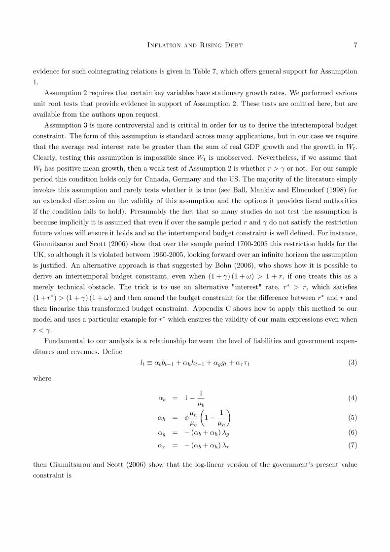
evidence for such cointegrating relations is given in Table 7, which o¤ers general support for Assumption
1.
Assumption 2 requires that certain key variables have stationary growth rates. We performed various
unit root tests that provide evidence in support of Assumption 2. These tests are omitted here, but are
available from the authors upon request.
Assumption 3 is more controversial and is critical in order for us to derive the intertemporal budget
constraint. The form of this assumption is standard across many applications, but in our case we require
that the average real interest rate be greater than the sum of real GDP growth and the growth in Wt.
Clearly, testing this assumption is impossible since Wt is unobserved. Nevertheless, if we assume that
Wt has positive mean growth, then a weak test of Assumption 2 is whether r > or not. For our sample
period this condition holds only for Canada, Germany and the US. The majority of the literature simply
invokes this assumption and rarely tests whether it is true (see Ball, Mankiw and Elmendorf (1998) for
an extended discussion on the validity of this assumption and the options it provides �scal authorities
if the condition fails to hold). Presumably the fact that so many studies do not test the assumption is
because implicitly it is assumed that even if over the sample period r and do not satisfy the restriction
future values will ensure it holds and so the intertemporal budget constraint is well de�ned. For instance,
Giannitsarou and Scott (2006) show that over the sample period 1700-2005 this restriction holds for the
UK, so although it is violated between 1960-2005, looking forward over an in�nite horizon the assumption
is justi�ed. An alternative approach is that suggested by Bohn (2006), who shows how it is possible to
derive an intertemporal budget constraint, even when (1 + ) (1 + !) > 1 + r, if one treats this as a
merely technical obstacle. The trick is to use an alternative "interest" rate, r� > r, which satis�es
(1+ r�) > (1 + ) (1 + !) and then amend the budget constraint for the di¤erence between r� and r and
then linearise this transformed budget constraint. Appendix C shows how to apply this method to our
model and uses a particular example for r� which ensures the validity of our main expressions even when
r < :
Fundamental to our analysis is a relationship between the level of liabilities and government expen-
ditures and revenues. De�ne
lt � �bbt�1 + �hht�1 + �ggt + ��� t (3)
where
�b = 1� 1
�b(4)
�h = ��h�b
�1� 1
�h
�(5)
�g = � (�b + �h)�g (6)
�� = � (�b + �h)�� (7)
then Giannitsarou and Scott (2006) show that the log-linear version of the government�s present value
constraint is

Inflation and Rising Debt 8
lt '��1� 1
�b
�+ �
�h�b
�1� 1
�h
��Et
1Xj=1
�1
�b
�j�dt+j +
�
�b(1� �h
�b)Et
1Xj=0
�1
�b
�j�ht+j
+
�1� 1
�b
�Et
T�1Xj=0
�1
�b
�j ��rt+j�1 + �
�h�b�t+j +
�1 + �
�h�b
� t+j
�: (8)
Note that by Assumption 3, it must be that �b > 1 and �h < 1:
The variable
dt � �ggt + ��� t;
where �g and �� are of opposite signs, is essentially a transformed version of the primary de�cit. The
critical variable for our analysis is lt, which is a measure of the imbalances in �scal policy. If �g > 0 and
�� < 0, then lt de�nes a relationship between government liabilities and the primary de�cit; if �g < 0
and �� > 0, then instead the relationship is between government liabilities and the primary surplus.
Since �b > 1 and �h < 1, the coe¢ cient on debt is positive and the coe¢ cient on money is negative,
regardless of the signs of �g and �� :
Equation (8) pins down a long run equilibrium relationship between the market value of government
debt, monetary liabilities and a version of the current primary de�cit, dt. We interpret this expression as
follows. For given values of mean interest rates, real GDP growth and money holdings, there has to be
a steady state relationship between debt and the primary de�cit, if debt is to be sustainable and for the
intertemporal budget constraint to hold. Under our Assumption 2 and given our empirical evidence on
unit roots, the right hand side of (8) is stationary, so that Etlt+j = �, as j !1; suggesting lt � � as anatural measure of required �scal adjustment. When lt = 0, then this equilibrium relationship holds, but
for lt > 0 debt is too high relative to current �scal de�cits. Adjustment is achieved through variations
in the right hand side of (8).
Further insights into (8) and lt can be gained from considering the results of Trehan and Walsh (1988)
and (1991), and Bohn (2006). The former show that the intertemporal budget constraint requires that
the primary de�cit and debt satisfy a cointegrating relationship. Given Assumption 2 and the fact that
Etlt+j = �, the same is true for our approximation to the intertemporal budget constraint.3 Bohn (2006)
focuses on an alternative insight, namely that debt sustainability requires a feedback rule from debt to
de�cits. Given Assumption 2, we know that lt must be stationary, which can be achieved through a
feedback rule from debt to the de�cit, although in this case the feedback is from a weighted average of
marketable debt and monetary liabilities.
If the left hand side of (8) measures the degree of �scal adjustment required, then the right hand side
of (8) tells us how this �scal adjustment (lt � �) is achieved through either: (a) future improvements inthe primary de�cit ��dt+j , (b) issuing more monetary liabilities, �ht+j or (c) variations in the growth
3Strictly speaking (8) states that if the components of lt are of order of integration N , then the right hand side of (8) isorder N � 1.

Inflation and Rising Debt 9
adjusted real interest rate (rt+j ��t+j � t+j). The coe¢ cients on each of the components of the growthadjusted real interest rate di¤er, as the nominal dividend e¤ect (�t+j � t+j) operates on both bondsand money, while rt+j a¤ects only bonds. As a result, equation (8) tells us that, if the intertemporal
budget constraint holds, any deviations in the long run relationship between debt and de�cits must help
predict movements in either future primary de�cits, money creation, nominal interest rates, in�ation or
GDP growth. We stress once more that our intertemporal budget constraint is an accounting framework
and the predictive role of lt is a purely statistical rather than necessarily causal phenomenon.
4. Estimating Fiscal Imbalances
Crucial to implementing our approach to the intertemporal budget constraint is construction of an
estimate for lt and so estimates of �b; �h; �g and �� :A common approach to estimating (3) and its
analogues in the literature is to use Stock and Watson�s (1993) Dynamic OLS estimator. In our case this
would involve estimating the regression:
gt = �1� t + �2bt�1 + �3ht�1 +kX
i=�k(ci��� t�i + cib�bt�i + cih�ht�i): (9)
Using (3), (4)-(7) and the fact that �g + �� = 1, we get the implied restrictions
�2 + �3 =1
1� ��; (10)
�1 = � ��1� ��
: (11)
Table 8 shows the results from estimating this equation and the implied estimated coe¢ cients for the
parameters of interest, �b, �h, �g and �� . These estimated coe¢ cients are calculated as follows. First, we
check that in each case, we cannot reject restriction (10), at either the 5% or 10% level. Next, equation
(9) contains three key estimated parameters, namely �1; �2 and �3. From these reduced form estimates
we wish to estimate the structural parameters �; �b; �h; �� , using relations (4)-(7). However, due to
(10), we have in e¤ect only two independently estimated parameters. Therefore identifying our structural
parameters requires using additional information. In particular, we can estimate � as the sample average
of narrow money to government debt ratio (H=B) and by de�nition we have �b=�h = (1 + �) (1 + r).
Using these additional restrictions we can then just identify the key structural parameters of interest and
construct our estimate of lt :
l̂t =
�1� 1
�b
�bt�1 + �
�h�b
�1� 1
�h
�ht�1 �
��1� 1
�b
�+ �
�h�b
�1� 1
�h
��dt:
The variable l̂t is a measure of the deviation of a weighted average of government liabilities from a
transformed measure of the primary de�cit dt. The larger lt is, the larger debt is relative to the steady
state level of de�cits and the greater the required degree of �scal adjustment. Note that given the
estimates of Table 8, the weights on government expenditure and tax revenue (�g and �� ) are of opposite

Inflation and Rising Debt 10
sign and approximately equal in absolute value, so that dt is only mildly di¤erent from the primary
de�cit (and in the case of Japan and the UK there is very little di¤erence). The coe¢ cients �g and
�� , re�ecting the relative importance of the primary de�cit relative to liabilities, clearly show signi�cant
variations across countries. These variations re�ect the fact that the size of the primary de�cit needed to
ensure sustainability depends on the level of interest rates, GDP growth and debt and small variations
in these numbers can produce large variations in �g and �� .
While this approach is standard in the literature our use of Assumption 1 creates additional problems
which make the above analysis problematic. Assumption 1 implies that Gt; Tt; Bt and Ht all share a
common stochastic trend, Wt. As a result there exist three (linearly independent) cointegrating vectors.
Evidence for this was shown in Table 7, which we used earlier as support for Assumption 1. In other
words, in our data we have the following cointegrating relationships:4
gt = '1tt + u1t
bt = '2ht + u2t
gt = '3bt + u3t
where uit; i = 1; 2; 3 are stationary error terms, since the variables cointegrate. Given that each of these
pairs is stationary, it also must be the case that any linear combination of these cointegrating relations
must also be stationary. In other words, Assumption 1 implies that for any �1; �2 and �3 the following
holds :
�1(gt � '1tt) + �2(bt � '2ht) + �3(gt � '3bt) = wt
where wt is a stationary error term which is a linear combination of the u0its. Rearranging this expression
yields
gt =�1'1�1 + �3
tt ��2 � �3'3�1 + �3
bt +�2'2�1 + �3
ht + wt
Assumption 1 implies that this equation must hold for arbitrary �1, �2 and �3 while the intertemporal
budget constraint implies, through (3), (4)-(7), that only one speci�c cointegrating vector is useful in
predicting future �scal behaviour e.g the right hand side of (8). Assumption 1 means that when we
estimate (3) using DOLS we are in e¤ect estimating some weighted average of the three cointegrating
vectors, where the weights are arbitrary and not uniquely determined. While (3) and (4)-(7) imply some
cross parameter restrictions, they are not enough to uniquely pin down �1; �2 and �3 and overcome
this indeterminacy. In other words, it is not obvious that the estimates in Table 8 truly uncover the
structural parameters that we are interested in.
4Here we follow Gourinchas and Rey (2005) and allow the coe¢ cients in these cointegrating relationships to di¤er from1. Measurement important when dealing with �scal data; in particular because of o¤-balance sheet items, o¢ cial debt datadoes not accumulate purely as a consequence of the total de�cit.

Inflation and Rising Debt 11
In order to validate the estimates of Table 8 as reliable measures of �scal imbalance, we use two
independent arguments. The �rst and most powerful is that the intertemporal budget constraint implies
more than just a linear cointegrating vector of the form (3) exists. In particular the intertemporal budget
constraint implies that the "true" lt, i.e. expression (3), equals the right hand side of (8). Assumption
1 entails that there exist many cointegrating vectors between bt; ht; gt and tt but the intertemporal
budget constraint implies that only one particular cointegrating vector should be useful in predicting the
present value of future �scal variables. This in turn implies that innovations in lt should be equal to the
innovations in the present value of these future �scal variables. We show in a later section how to exploit
this to test for the validity of our estimated (3) as a measure of �scal imbalances. For the cases where
this test is not rejected we can be con�dent that DOLS does not estimate an arbitrary cointegrating
relationship but the speci�c one implied by the intertemporal budget constraint.
The second means of verifying our DOLS estimates of (3) as a valid measure of �scal imbalances
is to provide alternative estimates of the key structural parameters �; �g; �� ; �b; �h and use these
to construct an estimate of fltg which can then be compared with those obtained from DOLS. Sample
estimates of real interest rates, real GDP growth, government expenditure, tax revenues and money
holdings as shares of GDP were constructed and an estimate of ! (the growth of the common trend Wt)
formed by averaging the trend growth rates of bt; ht; gt and tt. Estimating lt in this way is problematic
for several statistical reasons and is not our preferred approach. The �rst problem is that gt and tt are
non-stationary and so do not have a well de�ned unconditional mean. The second is that when we use
DOLS we can exploit the order of integration of the variables and arrive at superconsistent estimates.
However, this approach does o¤er, however �awed, a further means of assessing our measure of �scal
imbalances.
Table 9 shows the results for our key parameters from this alternative estimation method and also
o¤ers some information on how this measure of lt compares with that from using DOLS. For Canada,
UK and US the results are astoundingly similar, both in terms of the structural parameters and the
correlation between the estimates of lt and �lt. In all three cases we can reject strongly the null of
non-stationarity for this alternative estimate of lt. For Italy the coe¢ cient estimates are broadly similar
except that those on debt and money are around twice as large but the two estimates broadly track
one another and show similar behaviour in their rate of change. The only countries where there are
important di¤erences are for Japan and especially Germany, note that these are the two countries for
which our earlier analysis questioned the degree to which �scal policy had been sustainable over our
sample period. For Japan the main di¤erence is that the coe¢ cients on government expenditure and
taxation are much smaller than from DOLS and so this estimate of lt places much greater weight on
the debt and monetary liabilities term. This leads to a weaker correlation between the two estimates
although the �uctuations in lt are broadly similar. The two estimates for Germany are however very
di¤erent, with a near perfect negative correlation arising from the fact that �g and �t have opposite
signs to that from DOLS. Note also that there is only weak evidence that this alternative measure of ltis stationary, which our assumptions require. These independent validations of our DOLS estimates of

Inflation and Rising Debt 12
lt suggest that, with the exception of Germany, they are valid measures of the degree of �scal imbalance
as suggested by the intertemporal budget constraint.
We now move to consider in more detail what these estimates imply about the dynamics of �scal
adjustment. In order to make comparisons across countries it is necessary to standardise our measures of
lt, due to the fact that the estimated coe¢ cients in Table 8 di¤er so much across countries. As previously
described, l̂t is the deviation in the relationship between liabilities and the primary de�cit. Consider the
case where �scal equilibrium, i.e. lt = 0, is achieved purely through adjustments in tax rates. Given our
de�nition of lt this would require an increase in taxes of
l̂�t =1
���h�1� 1
�b
�+ ��h�b
�1� 1
�h
�i [l̂t �ml]:
where ml is the sample mean for lt and l̂�t is a normalised measure of �scal imbalances which can be
used to make comparisons across countries: it is the required increase in the tax revenue/GDP needed
to restore �scal equilibrium and can be thought of as an alternative measure of �scal sustainability to
those proposed by Blanchard et al (1989) and Polito and Wickens (2006).
Estimates of l̂�t are shown in Figure 3, for our sample period. These suggest that the discrepancy
between debt and de�cit in the US is currently on a par with the Reagan years, although it has shown
some signs of improvement over the last year. After a protracted correction during the 1980s and 1990s,
the estimates suggest that Canadian public �nances are now in rough balance as is German policy. Not
surprisingly Japan�s �scal situation has shown a dramatic recent deterioration, as has the �scal position
of UK. Finally, after many consecutive years of �scal improvements, our estimates suggest that from a
long term perspective, Italian public �nances have deteriorated signi�cantly in recent times. Table 10
reports some summary statistics regarding �scal adjustment for our countries during this period. The
degree of imbalance varies between around plus and minus 5% for all economies, except for the US where
the range is narrower (plus or minus 3%). In all cases �scal adjustment is highly persistent although
not a unit root process; as discussed above, it is critical for our analysis that lt is stationary. Fiscal
adjustment is a protracted process, with a half life of between 2 and 4 years. Given that our sample
period contains 46 years of data for most countries we have several completed cycles of �scal adjustment.
However, the case of Japan shows weakest evidence of adjustment in �scal policy, perhaps re�ecting our
earlier comments that the continual rise in Japanese government debt may re�ect an uncompleted �scal
adjustment.
5. Financing the Budget
The previous section constructed estimates of our measure of �scal imbalance and statistically charac-
terised its variability. Equation (8) states that these �uctuations in lt are associated with �uctuations
in future de�cits, money creation, real interest rates, in�ation and real GDP growth in a manner that
ensures the government�s intertemporal budget constraint holds. If the left hand side of 8) shows a
measure of �scal imbalance then the right hand side shows which variables account for variations in �scal

Inflation and Rising Debt 13
imbalances. We now turn our attention to using this equation to perform a variance decomposition on
lt. De�ne zt = (lt; �dt; �ht; rt�1; �t; t) and assume zt follows a VAR(p) process, i.e.
zt = A1zt�1 +A2zt�2 + :::+Apzt�p + "t;
where Ak; k = 1; :::; p are 6 � 6 matrices. Denoting zt =�z0t; z
0t�1; :::; z
0t�p+1
�and "t = ("0t; 0; :::; 0)
we can rewrite this VAR(p) as a VAR(1) so that
zt = Azt�1 + "t;
where
A =
0BBBB@A1 A2 � � � Ap�1 Ap
0 1 � � � 0 0...
.... . .
......
0 0 � � � 1 0
1CCCCA :Noting that conditional expectations satisfy
Etzt+j = Ajzt
and de�ning appropriate indicator vectors e such that
e0lzt = lt; e0�dzt = �dt; e
0rzt = rt�1; e
0�hzt = �ht; e
0�zt = �t; e
0 zt = t;
we can then, following Campbell and Shiller (1988) rewrite (8) as
e0lzt =
��1� 1
�b
�+ �
�h�b
�1� 1
�h
�� 1Xj=1
(1=�b)j e
0�dA
jzt +�
�b
�1� �h
�b
� 1Xj=0
(1=�b)j e
0�hA
jzt
��1� 1
�b
� 1Xj=0
(1=�b)j e
0rA
jzt +
�1� 1
�b
���h�b
1Xj=0
(1=�b)j e
0�A
jzt
+
�1� 1
�b
��1 + �
�h�b
� 1Xj=0
(1=�b)j e
0 A
jzt;
or equivalently
e0lzt =
(1
�b
��1� 1
�b
�+ �
�h�b
�1� 1
�h
��e0�dA
�I � 1
�bA
��1+�
�b
�1� �h
�b
�e0�h
�I � 1
�bA
��1��1� 1
�b
��e0r � �
�h�be0� �
�1 + �
�h�b
�e0
��I � 1
�bA
��1)zt: (12)

Inflation and Rising Debt 14
This is simply a restatement of our key equation (8), but where we have replaced the expectation
terms with conditional forecasts obtained from our VAR representation for zt. If our log linearisation to
the budget constraint is appropriate we have
e0l
�I � 1
�bA
�=
1
�b
��1� 1
�b
�+ �
�h�b
�1� 1
�h
��e0�dA+
�
�b
�1� �h
�b
�e0�h
��1� 1
�b
��e0r � �
�h�be0� �
�1 + �
�h�b
�e0
�: (13)
This expression shows the restriction our present value formula imposes on innovations to lt relative to
innovations in de�cits, money and growth adjusted real interest rates. It can therefore be used as a
joint test for the adequacy of both our approximation to the intertemporal budget constraint and the
forecasting system used for our variables. It is this test we referred to earlier as a means of validating
our DOLS estimates of lt. As shown in Giannitsarou and Scott (2006), an alternative and easier to
implement formulation of this restriction is:
0 = Et�1
�1
�b(�bt � ��ht) + lt �
�rt�1 � t � �
�h�b(�t + t)
��:
This last expression can be easily tested by regressing the expression in the expectation on variables in the
t-1 information set and testing for their signi�cance. If our log linear approximation to the intertemporal
budget constraint is to hold, then these lagged variables should be insigni�cant.
To proceed with our variance decomposition we rewrite our system as
lt = F�d;t + F�h;t + Fr;t + F�;t + F ;t;
where
F�d;t =1
�b
��1� 1
�b
�+ �
�h�b
�1� 1
�h
��e0�dA
�I � 1
�bA
��1zt;
F�h;t =�
�b
�1� �h
�b
�e0�h
�I � 1
�bA
��1zt;
Fr;t = ��1� 1
�b
�e0r
�I � 1
�bA
��1zt;
F�;t =
�1� 1
�b
���h�be0�
�I � 1
�bA
��1zt;
F ;t =
�1� 1
�b
��1 + �
�h�b
�e0
�I � 1
�bA
��1zt:
where Fj;t denotes the projected contribution of component j towards maintaining the intertemporal
Inflation and Rising Debt 15
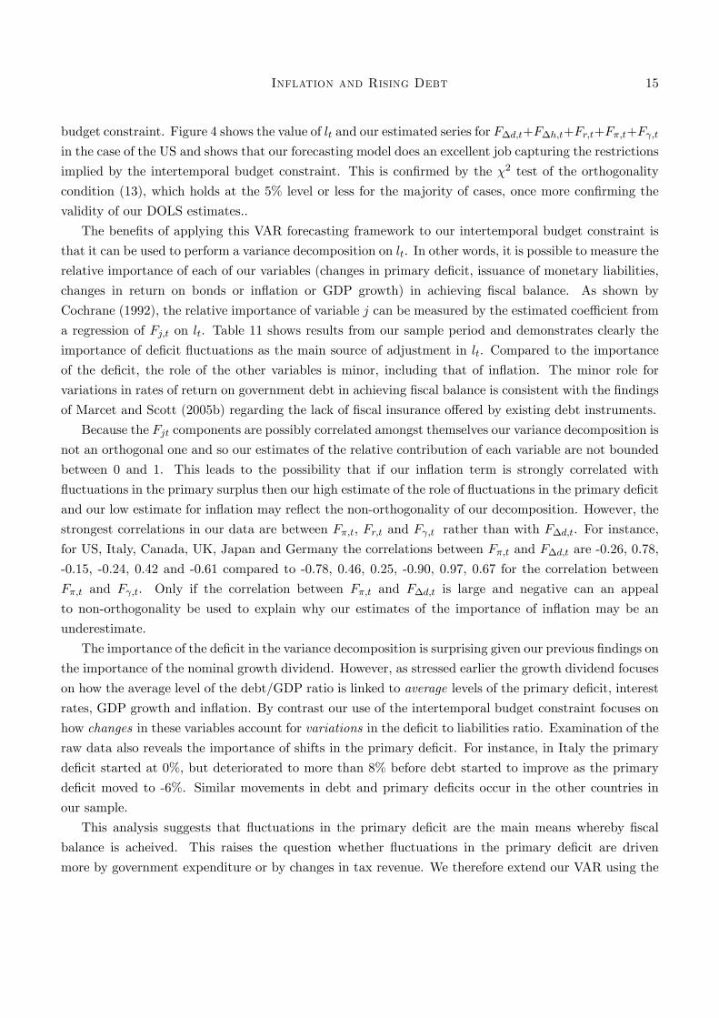
budget constraint. Figure 4 shows the value of lt and our estimated series for F�d;t+F�h;t+Fr;t+F�;t+F ;tin the case of the US and shows that our forecasting model does an excellent job capturing the restrictions
implied by the intertemporal budget constraint. This is con�rmed by the �2 test of the orthogonality
condition (13), which holds at the 5% level or less for the majority of cases, once more con�rming the
validity of our DOLS estimates..
The bene�ts of applying this VAR forecasting framework to our intertemporal budget constraint is
that it can be used to perform a variance decomposition on lt. In other words, it is possible to measure the
relative importance of each of our variables (changes in primary de�cit, issuance of monetary liabilities,
changes in return on bonds or in�ation or GDP growth) in achieving �scal balance. As shown by
Cochrane (1992), the relative importance of variable j can be measured by the estimated coe¢ cient from
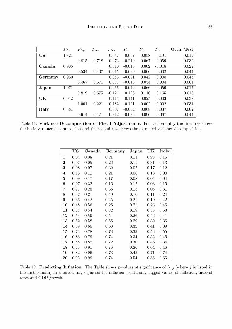
a regression of Fj;t on lt. Table 11 shows results from our sample period and demonstrates clearly the
importance of de�cit �uctuations as the main source of adjustment in lt. Compared to the importance
of the de�cit, the role of the other variables is minor, including that of in�ation. The minor role for
variations in rates of return on government debt in achieving �scal balance is consistent with the �ndings
of Marcet and Scott (2005b) regarding the lack of �scal insurance o¤ered by existing debt instruments.
Because the Fjt components are possibly correlated amongst themselves our variance decomposition is
not an orthogonal one and so our estimates of the relative contribution of each variable are not bounded
between 0 and 1. This leads to the possibility that if our in�ation term is strongly correlated with
�uctuations in the primary surplus then our high estimate of the role of �uctuations in the primary de�cit
and our low estimate for in�ation may re�ect the non-orthogonality of our decomposition. However, the
strongest correlations in our data are between F�;t, Fr;t and F ;t rather than with F�d;t. For instance,
for US, Italy, Canada, UK, Japan and Germany the correlations between F�;t and F�d;t are -0.26, 0.78,
-0.15, -0.24, 0.42 and -0.61 compared to -0.78, 0.46, 0.25, -0.90, 0.97, 0.67 for the correlation between
F�;t and F ;t. Only if the correlation between F�;t and F�d;t is large and negative can an appeal
to non-orthogonality be used to explain why our estimates of the importance of in�ation may be an
underestimate.
The importance of the de�cit in the variance decomposition is surprising given our previous �ndings on
the importance of the nominal growth dividend. However, as stressed earlier the growth dividend focuses
on how the average level of the debt/GDP ratio is linked to average levels of the primary de�cit, interest
rates, GDP growth and in�ation. By contrast our use of the intertemporal budget constraint focuses on
how changes in these variables account for variations in the de�cit to liabilities ratio. Examination of the
raw data also reveals the importance of shifts in the primary de�cit. For instance, in Italy the primary
de�cit started at 0%, but deteriorated to more than 8% before debt started to improve as the primary
de�cit moved to -6%. Similar movements in debt and primary de�cits occur in the other countries in
our sample.
This analysis suggests that �uctuations in the primary de�cit are the main means whereby �scal
balance is acheived. This raises the question whether �uctuations in the primary de�cit are driven
more by government expenditure or by changes in tax revenue. We therefore extend our VAR using the
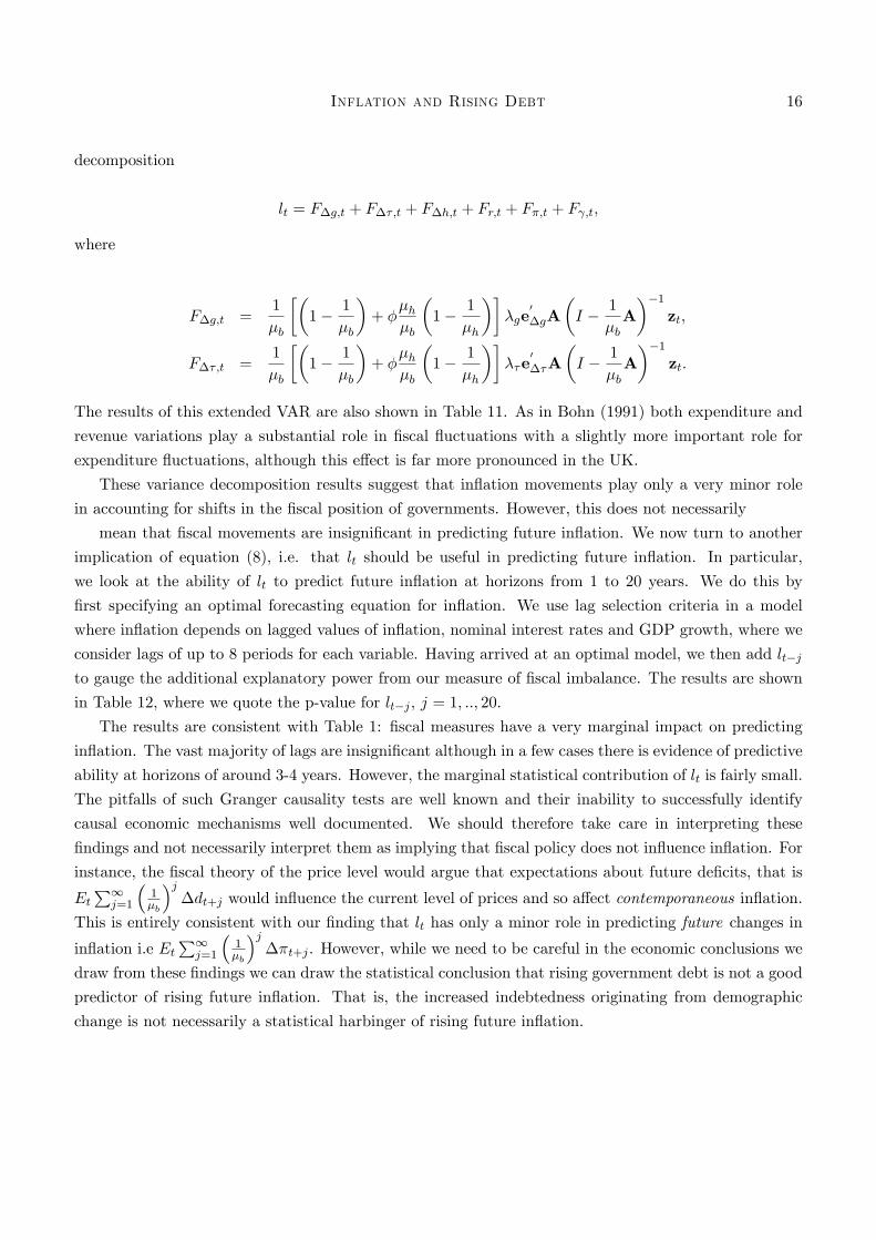
Inflation and Rising Debt 16
decomposition
lt = F�g;t + F��;t + F�h;t + Fr;t + F�;t + F ;t;
where
F�g;t =1
�b
��1� 1
�b
�+ �
�h�b
�1� 1
�h
���ge
0�gA
�I � 1
�bA
��1zt;
F��;t =1
�b
��1� 1
�b
�+ �
�h�b
�1� 1
�h
����e
0��A
�I � 1
�bA
��1zt:
The results of this extended VAR are also shown in Table 11. As in Bohn (1991) both expenditure and
revenue variations play a substantial role in �scal �uctuations with a slightly more important role for
expenditure �uctuations, although this e¤ect is far more pronounced in the UK.
These variance decomposition results suggest that in�ation movements play only a very minor role
in accounting for shifts in the �scal position of governments. However, this does not necessarily
mean that �scal movements are insigni�cant in predicting future in�ation. We now turn to another
implication of equation (8), i.e. that lt should be useful in predicting future in�ation. In particular,
we look at the ability of lt to predict future in�ation at horizons from 1 to 20 years. We do this by
�rst specifying an optimal forecasting equation for in�ation. We use lag selection criteria in a model
where in�ation depends on lagged values of in�ation, nominal interest rates and GDP growth, where we
consider lags of up to 8 periods for each variable. Having arrived at an optimal model, we then add lt�jto gauge the additional explanatory power from our measure of �scal imbalance. The results are shown
in Table 12, where we quote the p-value for lt�j ; j = 1; ::; 20.
The results are consistent with Table 1: �scal measures have a very marginal impact on predicting
in�ation. The vast majority of lags are insigni�cant although in a few cases there is evidence of predictive
ability at horizons of around 3-4 years. However, the marginal statistical contribution of lt is fairly small.
The pitfalls of such Granger causality tests are well known and their inability to successfully identify
causal economic mechanisms well documented. We should therefore take care in interpreting these
�ndings and not necessarily interpret them as implying that �scal policy does not in�uence in�ation. For
instance, the �scal theory of the price level would argue that expectations about future de�cits, that is
EtP1j=1
�1�b
�j�dt+j would in�uence the current level of prices and so a¤ect contemporaneous in�ation.
This is entirely consistent with our �nding that lt has only a minor role in predicting future changes in
in�ation i.e EtP1j=1
�1�b
�j��t+j . However, while we need to be careful in the economic conclusions we
draw from these �ndings we can draw the statistical conclusion that rising government debt is not a good
predictor of rising future in�ation. That is, the increased indebtedness originating from demographic
change is not necessarily a statistical harbinger of rising future in�ation.

Inflation and Rising Debt 17
6. Conclusion
This paper sought to apply a log linearised version of the intertemporal budget constraint to consider
government�s �scal positions. It tried to answer three key questions (a) is current �scal policy sustainable?
(b) how have OECD governments �nanced their �scal de�cits in recent decades and (c) what are the
implications for in�ation of the expected rising de�cits? The contribution of the paper is purely empirical,
using an accounting identity to quantify the statistical impact of certain key variables.
In answer to the �rst question, for each country we estimated a measure of current �scal imbalance,
de�ned as the ratio between current liabilities and the primary de�cit. For all countries, the current
measure for this imbalance was within the historical range of variation suggesting that current policies
are sustainable, with the possible exception of Japan. Using our version of the intertemporal budget
constraint, we analysed how in previous years governments had achieved �scal balance. We found an
overwhelming role for changes in the primary surplus with only a minor role for in�ation, growth and
interest rate e¤ects. Further we also found that �scal imbalances had only a very weak forecasting role
for future in�ation at nearly all horizons, with some mild evidence that �scal imbalances could help
predict in�ation three to four years ahead.
Obviously our results should be interpreted with care as they are based on a certain historical period
and an assumption that governments cannot take a de�cit gamble if r < ; inevitably any attempt at an
econometric approach to evaluating the intertemporal budget constraint is vulnerable to time dependence
and non-stationarity. Our accounting framework also prevents us from attributing any causal role to the
statistical relationships we discover. However, the statistical �ndings are striking: variations in �scal
imbalances and movements to �scal sustainability are achieved mainly through variations in the primary
de�cit. Moreover, rising government debt amongst these countries is not a reliable predictor of higher
future in�ation.
A. Data
Notes on data sources for the UK and US can be found in Giannitsarou and Scott (2006). For the
remaining countries details are as below. The following abbreviations are used:
� GFD: Global Financial Data
� IFS: International Financial Statistics (IMF)
� OECD-EO: OECD Economic Outlook Database
� OECD-CGD: OECD Central Government Debt Statistics
� HSoC: Historical Statistics of Canada ( Statistics Canada )
� DI: DataInsight

Inflation and Rising Debt 18
GDP, Prices and In�ation
Country variable sample period source ID/Speci�cation
CAN real GDP GFD GDPCCANM
nom. GDP GDPCANM
JAP nom. GDP 1955-2005 IFS 15899B.CZF
De�ator 15899BIRZF
JAP, ITA, GER nom. GDP 1960-2005 OECD-EO
De�ator
The implicit GDP de�ator is used as the price index.
(Gross) in�ation is then obtained as the annual rate of change of the index.
Base Money
Country sample source ID/Speci�cation
CAN 1926-1954 HSoC J69+J71
1955-2005 DI MBASENS@CN
GER DI M1@EURNS@GY
ITA 1960-1990 Fratianni (2005), p49¤ col BP
1991-2005 Banca d�Italia
JAP DI MBASENS@JP
For Canada, Italy, and Japan, base money is used.
For Germany, it is the national de�nition of M1 (currency in circulation plus overnight deposits).
Government receipts and expenditure
Country sample source ID/Spec.
CAN Receipts, expenditure 1926-1965 HSoC F109, F116
Receipts, expenditure 1966-2005 DI REVG@CN, EXG@CN
Interest EXGCDINS@CN
GER, ITA, JAP Receipts, expenditure OECD-EO
Interest
All government expenditure data is net of interest service. Revenues are net of interest receipts
for Germany, Italy and Japan, but not for Canada. The primary de�cit is expressed
as net expenditure minus (net) receipts.
Government debt and market values. Market values are approximated for central government
marketable debt, which is from OECD-CGD. For the periods before these data are available, the last
available share of marketable in total debt was used to obtain marketable debt. The price of government
debt is approximated as

Inflation and Rising Debt 19
pt =1 +NC
1 +NI;
where N is the average term to maturity of outstanding government securities, C is the average coupon
rate, and I is the average market yield. Data on average terms to maturity and average yields is from
OECD-CGD. If no average term to maturity was available, average maturities were used. For earlier
periods, the last average maturity available was taken. If average yields were unavailable, yields are
constant maturity benchmark yields (from GFD). For a given year, the benchmark yield closest to the
average term to maturity of that year was applied. Average coupon data is approximated as the ratio of
gross interest service to gross government debt, more precisely,
Ct =Interestt+1DEBTt
:

Inflation and Rising Debt 20
B. Variable Definitions and Notation
variable de�nition steady state
Gt government spending over GDPTt tax revenues over GDPBt debt over GDPHt seignorage over GDPWt aggregate wealthPt price indexYt real GDPRt = 1 + rt gross real interest rate R = 1 + r�t = 1 + it gross nominal interest rate � = 1 + i
t = WtWt�1
= 1 + !
�t = 1 + �t = PtPt�1
� = 1 + �
Qt = 1 + t = YtYt�1
Q = 1 + �Gt = Gt=Wt
�G�Tt = Tt=Wt
�T�Bt = Bt=Wt
�B�Ht = Ht=Wy
�Hwt = lnWt
gt = lnGt� t = lnTtbt = lnBtht = lnHtdt = �ggt + ��� t�b = �
�Q
�h = 1�Q
�g =�G
�G� �T�� = � �T
�G� �T� =
�H�B
m = (1� �b) �B + (1� �h) �Hml = samle mean of lt� = summary of constants that we can ignore

Inflation and Rising Debt 21
C. Derivation of the Log-Linear Budget Constraint5
The budget constraint for the government, after having adjusted with GDP and prices, can be written
as
Gt � Tt = Bt ��t�1�tQt
Bt�1 +Ht �1
�tQtHt�1:
Dividing through with Wt, we get
GtWt
� TtWt
=BtWt
� �t�1�tQtt
Bt�1Wt�1
+HtWt
� 1
�tQtt
Ht�1t�1
;
i.e.�Gt � �Tt = �Bt �
�t�1�tQtt
�Bt�1 + �Ht �1
�tQtt�Ht�1:
In this last expression, all variables are by assumption stationary. Thus we can log-linearise the expres-
sion. To do this, we rewrite it as
t �Gt � t �Tt = t �Bt ��t�1�tQt
�Bt�1 +t �Ht �1
�tQt�Ht�1;
We then use the approximations
exp(z) � z + 1;
rt�1 � it�1 + �t
and the steady state relationship
�G� �T = (1� �b) �B + (1� �h) �H � m or��G� �T
����B + �H
�= �
��b �B + �h �H
�;
to obtain
bt�1 =1
�bbt �
1
�b
m�Bdt +
�
�bst � rt�1 + �
�h�b�t +
�1 + �
�h�b
� t:
Substituting forward we get
bt�1 =
�1
�b
�Tbt+T�1 +
T�1Xj=0
�1
�b
�j �� 1
�b
m�Bdt+j +
�
�bst+j � rt+j�1 + �
�h�b�t+j +
�1 + �
�h�b
� t+j
�
Let
lt�1 =
�1� 1
�b
�bt�1 + �
�h�b
�1� 1
�h
�ht�1 �
��1� 1
�b
�+ �
�h�b
�1� 1
�h
��dt
5See Table ?? for the notation of the variables and parameters we use.
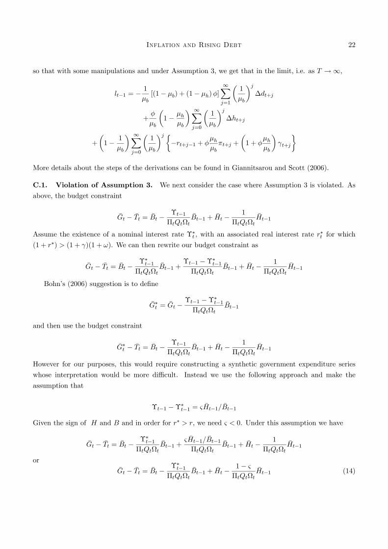
Inflation and Rising Debt 22
so that with some manipulations and under Assumption 3, we get that in the limit, i.e. as T !1,
lt�1 = �1
�b[(1� �b) + (1� �h)�]
1Xj=1
�1
�b
�j�dt+j
+�
�b
�1� �h
�b
� 1Xj=0
�1
�b
�j�ht+j
+
�1� 1
�b
� 1Xj=0
�1
�b
�j ��rt+j�1 + �
�h�b�t+j +
�1 + �
�h�b
� t+j
�
More details about the steps of the derivations can be found in Giannitsarou and Scott (2006).
C.1. Violation of Assumption 3. We next consider the case where Assumption 3 is violated. As
above, the budget constraint
�Gt � �Tt = �Bt ��t�1�tQtt
�Bt�1 + �Ht �1
�tQtt�Ht�1
Assume the existence of a nominal interest rate ��t , with an associated real interest rate r�t for which
(1 + r�) > (1 + )(1 + !). We can then rewrite our budget constraint as
�Gt � �Tt = �Bt ���t�1�tQtt
�Bt�1 +�t�1 ���t�1�tQtt
�Bt�1 + �Ht �1
�tQtt�Ht�1
Bohn�s (2006) suggestion is to de�ne
�G�t = �Gt ��t�1 ���t�1�tQtt
�Bt�1
and then use the budget constraint
�G�t � �Tt = �Bt ��t�1�tQtt
�Bt�1 + �Ht �1
�tQtt�Ht�1
However for our purposes, this would require constructing a synthetic government expenditure series
whose interpretation would be more di¢ cult. Instead we use the following approach and make the
assumption that
�t�1 ���t�1 = & �Ht�1= �Bt�1
Given the sign of H and B and in order for r� > r, we need & < 0. Under this assumption we have
�Gt � �Tt = �Bt ���t�1�tQtt
�Bt�1 +& �Ht�1= �Bt�1�tQtt
�Bt�1 + �Ht �1
�tQtt�Ht�1
or�Gt � �Tt = �Bt �
��t�1�tQtt
�Bt�1 + �Ht �1� &�tQtt
�Ht�1 (14)

Inflation and Rising Debt 23
This last equation is exactly the same as (2), except that the coe¢ cient on �Ht�1 is di¤erent. All the
above steps for deriving a log-linear present value constraint can now be replicated by substituting �band �h with
��b =1 + r�
(1 + ) (1 + !)and
��h =1� &
(1 + ) (1 + !)
respectively.

Inflation and Rising Debt 24
References
[1] Ball, Mankiw and Elmendorf, 1998, "The De�cit Gamble", Journal of Money, Credit, and Banking
30, 699 - 720.
[2] Bergin and She¤rin, 2000. "Interest Rates, Exchange Rates and Present Value Models of the Current
Account", Economic Journal 110, 535 - 558.
[3] Blanchard, Chouraqui, Hagemann, and Sartor, 1990. "The Sustainability of Fiscal Policy: New
Answers to Old Questions", OECD Economic Studies, 15.
[4] Bohn, 1991. "Budget Balance Through Revenue or Spending Adjustments? Some Historical Evi-
dence for the United States", Journal of Monetary Economics 27, 333-359.
[5] Bohn, 2005. "The Sustainability of Fiscal Policy in the United States", CESifo Working Paper 1446.
[6] Bohn, 2006. "Are stationarity and cointegration restrictions really necessary for the intertemporal
budget constraint?", Mimeograph.
[7] Campbell and Shiller, 1987. "Cointegration and Tests of Present Value Models", Journal of Political
Economy 95, 1062-88.
[8] Campbell and Shiller, 1988. "The Dividend-Price Ratio and Expectations of Future Dividends and
Discount Factors", Review of Financial Studies 1, 195-227.
[9] Campbell and Shiller, 1991. "Yield Spreads and Interest Rate Movements: A Bird�s Eye View",
Review of Economic Studies 58, 495-514.
[10] Cochrane, 1992. "Explaining the Variance of Price-Dividend Ratios", Review of Financial Studies
5, 243-80.
[11] Giannitsarou and Scott, 2006. "Paths to Fiscal Sustainability", mimeograph.
[12] Gourinchas and Rey, 2005. "International Financial Adjustment", NBER working paper 11155.
[13] Hansen, Roberds and Sargent, 1991. "Time-Series Implications of Present Value Budget Balance
and Martingale Models of Consumption and Taxes", in Rational Expectations Econometrics, edited
by Hansen and Sargent, Westview Press.
[14] Lettau and Ludvigson, 2001. "Consumption, Aggregate Wealth and Expected Stock Returns", Jour-
nal of Finance 56, 815-49.
[15] Leeper, 1991. "Equilibria under �active�and �passive�monetary and �scal policies", Journal of Mon-
etary Economics 27, 129-47.
[16] Marcet and Scott, 2005a. "Debt and De�cit Fluctuations and the Structure of Bond Markets�,
Mimeograph.
Inflation and Rising Debt 25
[17] Marcet and Scott, 2005b. "Fiscal Insurance and OECD Debt Management", Mimeograph.
[18] McCallum, 1984. "Are bond-�nanced de�cits in�ationary? A Ricardian analysis", Journal of Political
Economy 92, 123-35.
[19] Polito and Wickens, 2006. "Fiscal Policy Sustainability", Mimeograph.
[20] Roseveare, Leibfritz, Fore and Wurzel, 1998. "Ageing Populations, Pension Systems and Government
Budgets", OECD Economics Department Working Paper 168.
[21] Sargent and Wallace, 1981. "Some Unpleasant Monetarist Arithmetic", Federal Reserve Bank of
Minneapolis Quarterly Review.
[22] Sims, 1994. "A Simple Model for study of the determination of the price level and the interaction
of monetary and �scal policy", Economic Theory 4, 381-99.
[23] Stock and Watson, 1993. "A Simple Estimator of Cointegrating Vectors in Higher Order Integrated
Systems", Econometrica 61, 783-820.
[24] Trehan and Walsh, 1988. "Common Trends, the Government Budget Constraint and Revenue
Smoothing", Journal of Economic Dynamics and Control 12, 425-444.
[25] Trehan and Walsh, 1991. "Testing Intertemporal Budget Constraints: Theory and Application to
US Federal Budget and Current Account De�cits", Journal of Money, Banking and Credit 23, 206
- 223.
[26] Woodford, 1995. "Price level determinacy without control of a monetary aggregate", Carnegie
Rochester Conference Series on Public Policy 43, 1-46.
[27] Wickens and Uctum, 1993. "The Sustainability of Current Account De�cits: A Test of the US
Intertemporal Budget Constraint", Journal of Economic Dynamics and Control 17, 423 - 441.

Inflation and Rising Debt 26
Country Mean Min Max Initial Final St. Dev Feed Coef P-Value
Canada 0.378 0.292 0.718 0.292 0.464 0.193 -0.024 0.03Germany 0.246 0.049 0.700 0.052 0.700 0.213 -0.006 0.45Italy 0.702 0.304 1.203 0.374 1.076 0.328 -0.048 0.00Japan 0.333 0.041 1.296 0.069 1.296 0.226 -0.003 0.67UK 0.523 0.312 0.928 0.928 0.429 0.381 -0.034 0.01US 0.300 0.185 0.457 0.353 0.337 0.078 -0.057 0.01
Table 1: Debt Variability and Sustainability. First 5 columns report the average, minimum, max-imum, initial and �nal period values of the market value of government debt to GDP ratio. The nextcolumn reports the standard deviation of the debt/GDP ratio. The penultimate column shows estimatesof � in a regression of a country�s primary surplus on four lags of its own value and the lagged value ofthe debt/GDP ratio with the �nal column reporting the p value (to two decimal places) of the feedbackcoe¢ cient.

Inflation and Rising Debt 27
Debt/GDPCountry Test Statistic statistic 5% CV verdictCAN ADF(8) C -3.450 -2.860 stationary
ADF(8) C T -3.910 -3.410 trend stationaryKPSS(4) 0.718 0.463 unit rootKPSS(4) T 0.159 0.146 unit root
GER ADF(1) -2.280 -1.940 stationaryADF(1) C T -2.440 -3.410 unit rootKPSS(4) 0.994 0.460 unit rootKPSS(4) T 0.150 0.146 unit root
ITA ADF(1) -2.110 -1.940 stationaryKPSS(4) 0.959 0.463 unit rootKPSS(4) T 0.151 0.146 unit root
JAP ADF(1) -3.310 -1.940 stationaryADF(3) C T -2.270 -3.410 unit rootKPSS(4) 0.969 0.463 unit rootKPSS(4) T 0.163 0.146 unit root
UK ADF(2) C -2.510 -2.860 unit rootKPSS(4) 0.581 0.463 unit rootKPSS(4) T 0.204 0.146 unit root
US ADF(1) C -1.790 -2.860 unit rootADF(1) C T -2.440 -3.410 unit rootKPSS(4) 0.381 0.463 stationaryKPSS(4) T 0.146 0.146 unit root
C means constant included. T means trend included.
Table 2: Unit Root Tests, Gov Debt/GDP. ADF denotes Augmented Dickey Fuller Test and KPSSthe Kwiatowski, Phillips, Schmidt and Shin test. C denotes a constant also included in the test andT a trend. Number in parantheses indicates number of lags with which test was augmented. The �nalcolumn shows the inference from evaluating null of test statistic at 95 per cent con�dence intervals.

Inflation and Rising Debt 28
MoneyCountry test statistic 5% CV verdictCAN ADF(1) C -1.440 -2.860 unit root
KPSS(4) 0.971 0.463 unit rootKPSS(4) T 0.133 0.146 trend stationary
GER ADF(1) C 1.390 -2.860 unit rootADF(1) C T -1.110 -3.410 unit rootKPSS(4) 0.839 0.460 unit rootKPSS(4) T 0.253 0.146 unit root
ITA ADF(0) 1.410 -1.940 unit rootADF(4) C T -3.610 -3.410 trend stationaryKPSS(4) 0.880 0.463 unit rootKPSS(4) T 0.143 0.146 trend stationary
JAP ADF(1) -1.730 -1.940 unit rootKPSS(4) 0.590 0.463 unit rootKPSS(4) T 0.182 0.146 unit root
UK ADF(5) C -0.430 -1.940 unit rootKPSS(4) 0.940 0.463 unit rootKPSS(4) T 0.203 0.146 unit root
US ADF(1) C -2.080 -2.860 unit rootADF(0) C T -0.450 -3.410 unit rootKPSS(4) 0.666 0.463 unit rootKPSS(4) T 0.252 0.146 unit root
C means constant included. T means trend included.
Table 3: Unit Root Tests, H/GDP. The table reads as in table 2.

Inflation and Rising Debt 29
Expenditure/GDPCountry test statistic 5% CV verdictCAN ADF(1), C -2.110 -2.860 unit root
KPSS(4) 0.748 0.463 unit rootKPSS(4) T 0.217 0.146 unit root
GER ADF(0) -1.820 -1.940 unit rootKPSS(4) 0.600 0.460 unit rootKPSS(4) T 0.198 0.146 unit root
ITA ADF(2) C -2.670 -2.86 unit rootADF(2) C T -1.360 -3.410 unit rootKPSS(4) 0.920 0.463 unit rootKPSS(4) T 0.236 0.146 unit root
JAP ADF(3) -1.310 1.940 unit rootADF(3) C T -2.455 -3.410 unit rootKPSS(4) 0.941 0.463 unit rootKPSS(4) 0.137 0.146 trend stationary
UK ADF(9) C -1.604 -2.860 unit rootADF(10) C T -3.745 -3.410 trend stationaryKPSS(4) 0.398 0.463 stationaryKPSS(4) T 0.204 0.146 unit root
US ADF(7) C -1.628 -2.860 unit rootADF(6) C T -1.993 -3.410 trend stationaryKPSS(4) 0.193 0.463 stationaryKPSS(4) T 0.194 0.146 unit root
C means constant included. T means trend included.
Table 4: Unit Root Tests, G/GDP. The table reads as in table 2.
Inflation and Rising Debt 30
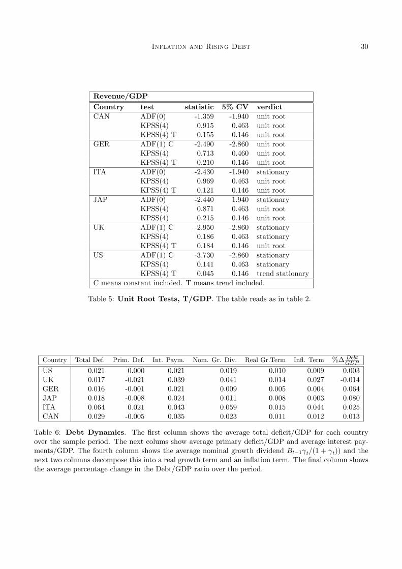
Revenue/GDPCountry test statistic 5% CV verdictCAN ADF(0) -1.359 -1.940 unit root
KPSS(4) 0.915 0.463 unit rootKPSS(4) T 0.155 0.146 unit root
GER ADF(1) C -2.490 -2.860 unit rootKPSS(4) 0.713 0.460 unit rootKPSS(4) T 0.210 0.146 unit root
ITA ADF(0) -2.430 -1.940 stationaryKPSS(4) 0.969 0.463 unit rootKPSS(4) T 0.121 0.146 unit root
JAP ADF(0) -2.440 1.940 stationaryKPSS(4) 0.871 0.463 unit rootKPSS(4) 0.215 0.146 unit root
UK ADF(1) C -2.950 -2.860 stationaryKPSS(4) 0.186 0.463 stationaryKPSS(4) T 0.184 0.146 unit root
US ADF(1) C -3.730 -2.860 stationaryKPSS(4) 0.141 0.463 stationaryKPSS(4) T 0.045 0.146 trend stationary
C means constant included. T means trend included.
Table 5: Unit Root Tests, T/GDP. The table reads as in table 2.
Country Total Def. Prim. Def. Int. Paym. Nom. Gr. Div. Real Gr.Term In�. Term %� DebtGDP
US 0.021 0.000 0.021 0.019 0.010 0.009 0.003UK 0.017 -0.021 0.039 0.041 0.014 0.027 -0.014GER 0.016 -0.001 0.021 0.009 0.005 0.004 0.064JAP 0.018 -0.008 0.024 0.011 0.008 0.003 0.080ITA 0.064 0.021 0.043 0.059 0.015 0.044 0.025CAN 0.029 -0.005 0.035 0.023 0.011 0.012 0.013
Table 6: Debt Dynamics. The �rst column shows the average total de�cit/GDP for each countryover the sample period. The next colums show average primary de�cit/GDP and average interest pay-ments/GDP. The fourth column shows the average nominal growth dividend Bt�1 t=(1 + t)) and thenext two columns decompose this into a real growth term and an in�ation term. The �nal column showsthe average percentage change in the Debt/GDP ratio over the period.

Inflation and Rising Debt 31
Gt; T t Gt; Bt Bt;Ht
Lags 0 1 2 3 4 0 1 2 3 4 0 1 2 3 4
Canada 1% 10% 5%� 5% 10% 1% 10%� 10% 5% 5% 5% 10%� 10%Germany 1% 10% 10% 10%� 5% 1%� 10% 10% 5% 5% 5% 10%� 10% 10%Italy 10% 5%� 5% 5% 1% 1%� 1% 1% 1% 1% 1%� 1% 1% 5%Japan 5% 10% 10%� 1% 1%� 1% 1% 1% 5% 5% 5%� 10% 10%UK 10% 10% 5%� 5% 5% 5% 5%� 1% 1% 5% 1% 5% 10%� 5% 5%US 5% 5%� 5% 1% 1% 1% 5% 5%� 5% 5% 1% 5% 1% 5%� 5%
Table 7: Cointegration tests. The Table shows the p-value of test for level of rejection of the null of nohypothesis between variables listed in top row using Johansen (1991). A � indicates the lag augmentationselected by the AIC criteria.
US Canada Germany Japan UK Italy� 0.302 0.174 1.060 0.612 0.103 0.267 1.078 1.083 1.065 1.057 1.090 1.075�b 1.027 1.033 1.008 1.021 1.008 1.041�h 0.953 0.954 0.947 0.965 0.925 0.969�g -6.968 -15.650 7.690 -2564.103 -56.526 -3.073�� 7.968 16.650 -6.690 2565.103 57.526 4.073�b 0.026 0.032 0.008 0.020 0.008 0.040�h -0.014 -0.008 -0.056 -0.021 -0.008 -0.008�g 0.088 0.376 0.376 -1.458 0.047 0.097�� -0.100 -0.399 -0.319 1.458 -0.048 -0.129H0 : �2 + �3 =
11��� 0.033 0.046 0.071 0.029 0.061 0.039
Table 8: Estimates of Equilibrium Relationship Debt and De�cits. The �rst row reports thesample average of H=B and the second row reports the sample average of nominal GDP growth. Theparameters �b and �� are estimated, as are �g and �� (subject to the restriction that �g +�� = 1). Thenext four rows show the implied estimated coe¢ cients for de�ning lt = �bbt + �hht + �ggt + ��� t. Thelast row shows p-values for the hypothesis that �2 + �3 = 1=(1� �� ).

Inflation and Rising Debt 32
US Japan Germany UK Italy Canada�b 1.026 1.015 1.006 1.008 1.010 1.014
1.027 1.021 1.008 1.008 1.041 1.033�h 0.947 0.980 0.973 0.933 0.944 0.978
0.953 0.965 0.947 0.925 0.969 0.954�g -9.371 34.703 -19.672 -52.589 20.196 -36.460
-6.968 -2564.100 7.690 -56.526 -3.073 -15.650�t 10.371 -33.703 20.672 53.589 -19.196 37.460
7.968 2565.100 -6.690 57.526 4.073 16.650�b 0.026 0.015 0.006 0.008 0.010 0.014
0.026 0.020 0.008 0.008 0.004 0.032�h -0.016 -0.012 -0.028 -0.007 -0.015 -0.004
-0.014 -0.021 -0.056 -0.008 -0.008 -0.008�g 0.095 -0.093 -0.441 0.040 0.105 0.383
0.088 -1.458 0.376 0.047 0.097 0.376�t -0.105 0.089 0.464 -0.041 -0.100 -0.394
-0.100 1.458 -0.319 -0.048 -0.129 -0.399
Corr(lt) 0.999 0.874 -0.978 0.999 0.749 0.966Corr(�lt) 0.998 0.893 -0.617 0.998 0.824 0.997ADF 0.010 0.030 0.080 0.010 0.030 0.010
Table 9: Alternative Estimates of Fiscal Imbalances. The �rst row for each country shows es-timates of structural parameters and coe¢ cients to form lt using sample averages and the second rowshows estimates from DOLS. The row labelled Corr(lt) shows the correlation coe¢ cient between the twoestimates of lt and the row labelled Corr(�lt) shows the correlation between the �rst di¤erences of thetwo estimates. The �nal row shows the p-value from an Augmented Dickey Fuller test for stationarity.
US Canada Germany Japan UK ItalyMax 0.031 0.065 0.050 0.045 0.055 0.049Min -0.025 -0.053 -0.053 -0.060 -0.049 -0.062Std Dev 0.015 0.027 0.022 0.027 0.024 0.026Sum AR 0.758 0.860 0.718 0.608 0.756 0.590Unit Root 0.042 0.031 0.100 0.046 0.054 0.02725% 0.960 3.300 0.930 1.300 0.210 3.00050% 2.500 4.100 2.100 2.100 2.500 4.10075% 5.000 5.200 4.100 2.900 4.960 6.900
Table 10: Dynamics of Fiscal Adjustment. The �rst row shows minimum value of lt over sampleperiod, while the second row shows the maximum value. The third row is the standard deviation of ltand the fourth row shows the sum of the AR coe¢ cients when lt is modelled as an AR(P) process whereP is chosen optimally using AIC criteria. The next row is the p-value from an ADF test that lt is a unitroot process. The last three rows show the number of periods it takes lt to adjust by 25%, 50% and 75%respectively to a shock to its value.
Inflation and Rising Debt 33
F�d F�g F�� F�h Fr F� F Orth. TestUS 1.321 -0.057 0.007 0.058 0.191 0.019
0.815 0.718 0.073 -0.219 0.067 -0.059 0.032Canada 0.985 0.010 -0.013 0.002 -0.018 0.022
0.534 -0.437 -0.015 -0.039 0.006 -0.002 0.044Germany 0.930 0.053 -0.021 0.042 0.008 0.045
0.467 0.571 0.021 -0.016 0.034 0.004 0.061Japan 1.071 -0.066 0.042 0.066 0.059 0.017
0.819 0.675 -0.121 0.126 0.116 0.165 0.013UK 0.912 0.113 -0.141 0.025 -0.003 0.038
1.001 0.221 0.182 -0.121 -0.002 -0.002 0.031Italy 0.881 0.007 -0.054 0.068 0.037 0.062
0.614 0.471 0.312 -0.036 0.096 0.067 0.044
Table 11: Variance Decomposition of Fiscal Adjustments. For each country the �rst row showsthe basic variance decomposition and the second row shows the extended variance decomposition.
US Canada Germany Japan UK Italy1 0.04 0.08 0.21 0.13 0.23 0.162 0.07 0.05 0.26 0.11 0.31 0.133 0.08 0.07 0.32 0.07 0.17 0.124 0.13 0.11 0.21 0.06 0.13 0.085 0.09 0.17 0.17 0.08 0.04 0.046 0.07 0.32 0.16 0.12 0.03 0.157 0.21 0.25 0.35 0.15 0.05 0.318 0.32 0.21 0.49 0.16 0.11 0.249 0.36 0.42 0.45 0.21 0.19 0.4210 0.48 0.56 0.26 0.21 0.23 0.4611 0.63 0.54 0.32 0.19 0.35 0.5312 0.54 0.59 0.54 0.26 0.46 0.4113 0.52 0.58 0.56 0.29 0.32 0.3614 0.59 0.65 0.63 0.32 0.41 0.3915 0.73 0.78 0.78 0.33 0.53 0.5516 0.86 0.79 0.74 0.34 0.52 0.4517 0.88 0.82 0.72 0.30 0.46 0.3418 0.75 0.91 0.76 0.26 0.64 0.4619 0.82 0.96 0.73 0.45 0.71 0.7420 0.95 0.99 0.74 0.54 0.55 0.65
Table 12: Predicting In�ation. The Table shows p-values of signi�cance of lt�j (where j is listed inthe �rst column) in a forecasting equation for in�ation, containing lagged values of in�ation, interestrates and GDP growth.

Inflation and Rising Debt 34
Figure 1: Debt over GDP, for six industrialised countries, 1960 - 2005.
Figure 2: Total de�cit over GDP, for six industrialised countries, 1960 - 2005.

Inflation and Rising Debt 35
Figure 3: Fiscal Position.

Inflation and Rising Debt 36
Figure 4: US Decomposition.