nag library chapter introduction f08 – least squares and ...2.2.1 qr factorization the most...

NAG Library Chapter Introduction

f08 – Least Squares and Eigenvalue Problems (LAPACK)

Contents

1 Scope of the Chapter . . . . . . . . . . . . . . . . . . . . . . . . . . . . . . . . . . . . . . . . . . . . . . . . . . . . 3

2 Background to the Problems . . . . . . . . . . . . . . . . . . . . . . . . . . . . . . . . . . . . . . . . . . . . 3

2.1 Linear Least Squares Problems. . . . . . . . . . . . . . . . . . . . . . . . . . . . . . . . . . . . . . . . . . 3

2.2 Orthogonal Factorizations and Least Squares Problems . . . . . . . . . . . . . . . . . . . . . 4

2.2.1 QR factorization . . . . . . . . . . . . . . . . . . . . . . . . . . . . . . . . . . . . . . . . . . . . . . . . . . 42.2.2 LQ factorization . . . . . . . . . . . . . . . . . . . . . . . . . . . . . . . . . . . . . . . . . . . . . . . . . . 52.2.3 QR factorization with column pivoting. . . . . . . . . . . . . . . . . . . . . . . . . . . . . . . . . 52.2.4 Complete orthogonal factorization . . . . . . . . . . . . . . . . . . . . . . . . . . . . . . . . . . . . . 62.2.5 Updating a QR factorization . . . . . . . . . . . . . . . . . . . . . . . . . . . . . . . . . . . . . . . . . 62.2.6 Other factorizations . . . . . . . . . . . . . . . . . . . . . . . . . . . . . . . . . . . . . . . . . . . . . . . . 7

2.3 The Singular Value Decomposition . . . . . . . . . . . . . . . . . . . . . . . . . . . . . . . . . . . . . . 7

2.4 The Singular Value Decomposition and Least Squares Problems . . . . . . . . . . . . . 8

2.5 Generalized Linear Least Squares Problems . . . . . . . . . . . . . . . . . . . . . . . . . . . . . . . 8

2.6 Generalized Orthogonal Factorization and Generalized Linear Least SquaresProblems . . . . . . . . . . . . . . . . . . . . . . . . . . . . . . . . . . . . . . . . . . . . . . . . . . . . . . . . . . . . 8

2.6.1 Generalized QR Factorization . . . . . . . . . . . . . . . . . . . . . . . . . . . . . . . . . . . . . . . . 82.6.2 Generalized RQ Factorization . . . . . . . . . . . . . . . . . . . . . . . . . . . . . . . . . . . . . . . . 92.6.3 Generalized Singular Value Decomposition (GSVD) . . . . . . . . . . . . . . . . . . . . . . 112.6.4 The Full CS Decomposition of Orthogonal Matrices . . . . . . . . . . . . . . . . . . . . . 12

2.7 Symmetric Eigenvalue Problems. . . . . . . . . . . . . . . . . . . . . . . . . . . . . . . . . . . . . . . . 13

2.8 Generalized Symmetric-definite Eigenvalue Problems . . . . . . . . . . . . . . . . . . . . . . 14

2.9 Packed Storage for Symmetric Matrices . . . . . . . . . . . . . . . . . . . . . . . . . . . . . . . . . 14

2.10 Band Matrices . . . . . . . . . . . . . . . . . . . . . . . . . . . . . . . . . . . . . . . . . . . . . . . . . . . . . . . 14

2.11 Nonsymmetric Eigenvalue Problems . . . . . . . . . . . . . . . . . . . . . . . . . . . . . . . . . . . . 15

2.12 Generalized Nonsymmetric Eigenvalue Problem . . . . . . . . . . . . . . . . . . . . . . . . . . 16

2.13 The Sylvester Equation and the Generalized Sylvester Equation . . . . . . . . . . . . . 17

2.14 Error and Perturbation Bounds and Condition Numbers . . . . . . . . . . . . . . . . . . . . 17

2.14.1 Least squares problems . . . . . . . . . . . . . . . . . . . . . . . . . . . . . . . . . . . . . . . . . . . . 182.14.2 The singular value decomposition . . . . . . . . . . . . . . . . . . . . . . . . . . . . . . . . . . . . 192.14.3 The symmetric eigenproblem. . . . . . . . . . . . . . . . . . . . . . . . . . . . . . . . . . . . . . . . 202.14.4 The generalized symmetric-definite eigenproblem . . . . . . . . . . . . . . . . . . . . . . . . 212.14.5 The nonsymmetric eigenproblem. . . . . . . . . . . . . . . . . . . . . . . . . . . . . . . . . . . . . 212.14.6 Balancing and condition for the nonsymmetric eigenproblem . . . . . . . . . . . . . . . 222.14.7 The generalized nonsymmetric eigenvalue problem. . . . . . . . . . . . . . . . . . . . . . . 222.14.8 Balancing the generalized eigenvalue problem . . . . . . . . . . . . . . . . . . . . . . . . . . 232.14.9 Other problems . . . . . . . . . . . . . . . . . . . . . . . . . . . . . . . . . . . . . . . . . . . . . . . . . . 23

2.15 Block Partitioned Algorithms . . . . . . . . . . . . . . . . . . . . . . . . . . . . . . . . . . . . . . . . . . 23

f08 – Least-squares and Eigenvalue Problems (LAPACK) Introduction – f08

Mark 25 f08.1

3 Recommendations on Choice and Use of Available Functions . . . . . . . . . . . 24

3.1 Available Functions . . . . . . . . . . . . . . . . . . . . . . . . . . . . . . . . . . . . . . . . . . . . . . . . . . 24

3.1.1 Driver functions . . . . . . . . . . . . . . . . . . . . . . . . . . . . . . . . . . . . . . . . . . . . . . . . . 243.1.1.1 Linear least squares problems (LLS). . . . . . . . . . . . . . . . . . . . . . . . . . . . 243.1.1.2 Generalized linear least squares problems (LSE and GLM) . . . . . . . . . . 243.1.1.3 Symmetric eigenvalue problems (SEP) . . . . . . . . . . . . . . . . . . . . . . . . . . 243.1.1.4 Nonsymmetric eigenvalue problem (NEP). . . . . . . . . . . . . . . . . . . . . . . . 253.1.1.5 Singular value decomposition (SVD) . . . . . . . . . . . . . . . . . . . . . . . . . . . 253.1.1.6 Generalized symmetric definite eigenvalue problems (GSEP) . . . . . . . . . 253.1.1.7 Generalized nonsymmetric eigenvalue problem (GNEP) . . . . . . . . . . . . . 263.1.1.8 Generalized singular value decomposition (GSVD). . . . . . . . . . . . . . . . . 26

3.1.2 Computational functions . . . . . . . . . . . . . . . . . . . . . . . . . . . . . . . . . . . . . . . . . . . 263.1.2.1 Orthogonal factorizations . . . . . . . . . . . . . . . . . . . . . . . . . . . . . . . . . . . . 263.1.2.2 Generalized orthogonal factorizations . . . . . . . . . . . . . . . . . . . . . . . . . . . 273.1.2.3 Singular value problems . . . . . . . . . . . . . . . . . . . . . . . . . . . . . . . . . . . . . 273.1.2.4 Generalized singular value decomposition. . . . . . . . . . . . . . . . . . . . . . . . 283.1.2.5 Symmetric eigenvalue problems . . . . . . . . . . . . . . . . . . . . . . . . . . . . . . . 283.1.2.6 Generalized symmetric-definite eigenvalue problems. . . . . . . . . . . . . . . . 303.1.2.7 Nonsymmetric eigenvalue problems . . . . . . . . . . . . . . . . . . . . . . . . . . . . 313.1.2.8 Generalized nonsymmetric eigenvalue problems . . . . . . . . . . . . . . . . . . . 323.1.2.9 The Sylvester equation and the generalized Sylvester equation . . . . . . . 33

3.2 NAG Names and LAPACK Names . . . . . . . . . . . . . . . . . . . . . . . . . . . . . . . . . . . . . 34

3.3 Matrix Storage Schemes . . . . . . . . . . . . . . . . . . . . . . . . . . . . . . . . . . . . . . . . . . . . . . 35

3.3.1 Conventional storage . . . . . . . . . . . . . . . . . . . . . . . . . . . . . . . . . . . . . . . . . . . . . . 353.3.2 Packed storage . . . . . . . . . . . . . . . . . . . . . . . . . . . . . . . . . . . . . . . . . . . . . . . . . . 353.3.3 Band storage . . . . . . . . . . . . . . . . . . . . . . . . . . . . . . . . . . . . . . . . . . . . . . . . . . . . 353.3.4 Tridiagonal and bidiagonal matrices . . . . . . . . . . . . . . . . . . . . . . . . . . . . . . . . . . 353.3.5 Real diagonal elements of complex matrices. . . . . . . . . . . . . . . . . . . . . . . . . . . . 353.3.6 Representation of orthogonal or unitary matrices . . . . . . . . . . . . . . . . . . . . . . . . 35

3.4 Argument Conventions. . . . . . . . . . . . . . . . . . . . . . . . . . . . . . . . . . . . . . . . . . . . . . . . 36

3.4.1 Option arguments . . . . . . . . . . . . . . . . . . . . . . . . . . . . . . . . . . . . . . . . . . . . . . . . 363.4.2 Problem dimensions . . . . . . . . . . . . . . . . . . . . . . . . . . . . . . . . . . . . . . . . . . . . . . 36

4 Decision Trees . . . . . . . . . . . . . . . . . . . . . . . . . . . . . . . . . . . . . . . . . . . . . . . . . . . . . . . . . . 37

4.1 General Purpose Functions (eigenvalues and eigenvectors) . . . . . . . . . . . . . . . . . 37

4.2 General Purpose Functions (singular value decomposition) . . . . . . . . . . . . . . . . . 42

5 Functionality Index. . . . . . . . . . . . . . . . . . . . . . . . . . . . . . . . . . . . . . . . . . . . . . . . . . . . . 42

6 Auxiliary Functions Associated with Library Function Arguments . . . . . . 49

7 Functions Withdrawn or Scheduled for Withdrawal . . . . . . . . . . . . . . . . . . . . 49

8 References. . . . . . . . . . . . . . . . . . . . . . . . . . . . . . . . . . . . . . . . . . . . . . . . . . . . . . . . . . . . . . 49

Introduction – f08 NAG Library Manual

f08.2 Mark 25

1 Scope of the Chapter

This chapter provides functions for the solution of linear least squares problems, eigenvalue problemsand singular value problems, as well as associated computations. It provides functions for:

– solution of linear least squares problems

– solution of symmetric eigenvalue problems

– solution of nonsymmetric eigenvalue problems

– solution of singular value problems

– solution of generalized linear least squares problems

– solution of generalized symmetric-definite eigenvalue problems

– solution of generalized nonsymmetric eigenvalue problems

– solution of generalized singular value problems

– matrix factorizations associated with the above problems

– estimating condition numbers of eigenvalue and eigenvector problems

– estimating the numerical rank of a matrix

– solution of the Sylvester matrix equation

Functions are provided for both real and complex data.

For a general introduction to the solution of linear least squares problems, you should turn first toChapter f04. The decision trees, at the end of Chapter f04, direct you to the most appropriate functionsin Chapters f04 or f08. Chapters f04 and f08 contain Black Box (or driver) functions which enablestandard linear least squares problems to be solved by a call to a single function.

For a general introduction to eigenvalue and singular value problems, you should turn first to Chapterf02. The decision trees, at the end of Chapter f02, direct you to the most appropriate functions inChapters f02 or f08. Chapters f02 and f08 contain Black Box (or driver) functions which enable standardtypes of problem to be solved by a call to a single function. Often functions in Chapter f02 call Chapterf08 functions to perform the necessary computational tasks.

The functions in this chapter (Chapter f08) handle only dense, band, tridiagonal and Hessenberg matrices(not matrices with more specialised structures, or general sparse matrices). The tables in Section 3 andthe decision trees in Section 4 direct you to the most appropriate functions in Chapter f08.

The functions in this chapter have all been derived from the LAPACK project (see Anderson et al.(1999)). They have been designed to be efficient on a wide range of high-performance computers,without compromising efficiency on conventional serial machines.

It is not expected that you will need to read all of the following sections, but rather you will pick outthose sections relevant to your particular problem.

2 Background to the Problems

This section is only a brief introduction to the numerical solution of linear least squares problems,eigenvalue and singular value problems. Consult a standard textbook for a more thorough discussion, forexample Golub and Van Loan (2012).

2.1 Linear Least Squares Problems

The linear least squares problem is

minimizex

b�Axk k2; ð1Þ

where A is an m by n matrix, b is a given m element vector and x is an n-element solution vector.


Mark 25 f08.3

In the most usual case m � n and rank Að Þ ¼ n, so that A has full rank and in this case the solution toproblem (1) is unique; the problem is also referred to as finding a least squares solution to anoverdetermined system of linear equations.

When m < n and rank Að Þ ¼ m, there are an infinite number of solutions x which exactly satisfyb�Ax ¼ 0. In this case it is often useful to find the unique solution x which minimizes xk k2, and theproblem is referred to as finding a minimum norm solution to an underdetermined system of linearequations.

In the general case when we may have rank Að Þ < min m;nð Þ – in other words, A may be rank-deficient– we seek the minimum norm least squares solution x which minimizes both xk k2 and b�Axk k2.

This chapter (Chapter f08) contains driver functions to solve these problems with a single call, as well ascomputational functions that can be combined with functions in Chapter f07 to solve these linear leastsquares problems. The next two sections discuss the factorizations that can be used in the solution oflinear least squares problems.

2.2 Orthogonal Factorizations and Least Squares Problems

A number of functions are provided for factorizing a general rectangular m by n matrix A, as theproduct of an orthogonal matrix (unitary if complex) and a triangular (or possibly trapezoidal) matrix.

A real matrix Q is orthogonal if QTQ ¼ I; a complex matrix Q is unitary if QHQ ¼ I. Orthogonal orunitary matrices have the important property that they leave the 2-norm of a vector invariant, so that

xk k2 ¼ Qxk k2;

if Q is orthogonal or unitary. They usually help to maintain numerical stability because they do notamplify rounding errors.

Orthogonal factorizations are used in the solution of linear least squares problems. They may also beused to perform preliminary steps in the solution of eigenvalue or singular value problems, and areuseful tools in the solution of a number of other problems.

2.2.1 QR factorization

The most common, and best known, of the factorizations is the QR factorization given by

A ¼ Q R0

� �; if m � n;

where R is an n by n upper triangular matrix and Q is an m by m orthogonal (or unitary) matrix. If A isof full rank n, then R is nonsingular. It is sometimes convenient to write the factorization as

A ¼ Q1Q2ð Þ R0

� �

which reduces to

A ¼ Q1R;

where Q1 consists of the first n columns of Q, and Q2 the remaining m� n columns.

If m < n, R is trapezoidal, and the factorization can be written

A ¼ Q R1R2ð Þ; if m < n;

where R1 is upper triangular and R2 is rectangular.

The QR factorization can be used to solve the linear least squares problem (1) when m � n and A is offull rank, since

b�Axk k2 ¼ QTb�QTAx��

2¼ c1 �Rx

c2

� ��

2

;

where


f08.4 Mark 25

c � c1

c2

� �¼

QT1b

QT2b

0@

1A ¼ QTb;

and c1 is an n-element vector. Then x is the solution of the upper triangular system

Rx ¼ c1:

The residual vector r is given by

r ¼ b�Ax ¼ Q 0c2

� �:

The residual sum of squares rk k22 may be computed without forming r explicitly, since

rk k2 ¼ b�Axk k2 ¼ c2k k2:

2.2.2 LQ factorization

The LQ factorization is given by

A ¼ L 0ð ÞQ ¼ L 0ð Þ Q1

Q2

� �¼ LQ1; if m � n;

where L is m by m lower triangular, Q is n by n orthogonal (or unitary), Q1 consists of the first m rowsof Q, and Q2 the remaining n�m rows.

The LQ factorization of A is essentially the same as the QR factorization of AT (AH if A is complex),since

A ¼ L 0ð ÞQ, AT ¼ QT LT

0

� �:

The LQ factorization may be used to find a minimum norm solution of an underdetermined system oflinear equations Ax ¼ b where A is m by n with m < n and has rank m. The solution is given by

x ¼ QT L�1b0

� �:

2.2.3 QR factorization with column pivoting

To solve a linear least squares problem (1) when A is not of full rank, or the rank of A is in doubt, wecan perform either a QR factorization with column pivoting or a singular value decomposition.

The QR factorization with column pivoting is given by

A ¼ Q R0

� �PT; m � n;

where Q and R are as before and P is a (real) permutation matrix, chosen (in general) so that

r11j j � r22j j � � � � � rnnj j

and moreover, for each k,

rkkj j � Rk:j;j

�� 2; j ¼ kþ 1; . . . ; n:

If we put

R ¼ R11 R12

0 R22

� �

where R11 is the leading k by k upper triangular sub-matrix of R then, in exact arithmetic, ifrank Að Þ ¼ k, the whole of the sub-matrix R22 in rows and columns kþ 1 to n would be zero. Innumerical computation, the aim must be to determine an index k, such that the leading sub-matrix R11 is


Mark 25 f08.5

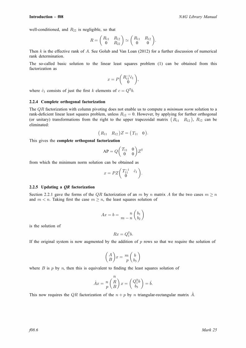
well-conditioned, and R22 is negligible, so that

R ¼ R11 R12

0 R22

� �’ R11 R12

0 0

� �:

Then k is the effective rank of A. See Golub and Van Loan (2012) for a further discussion of numericalrank determination.

The so-called basic solution to the linear least squares problem (1) can be obtained from thisfactorization as

x ¼ P R�111 c1

0

� �;

where c1 consists of just the first k elements of c ¼ QTb.

2.2.4 Complete orthogonal factorization

The QR factorization with column pivoting does not enable us to compute a minimum norm solution to arank-deficient linear least squares problem, unless R12 ¼ 0. However, by applying for further orthogonal(or unitary) transformations from the right to the upper trapezoidal matrix R11 R12

� �, R12 can be

eliminated:

R11 R12

� �Z ¼ T11 0

� �:

This gives the complete orthogonal factorization

AP ¼ Q T11 00 0

� �ZT

from which the minimum norm solution can be obtained as

x ¼ PZ T�111 c1

0

� �:

2.2.5 Updating a QR factorization

Section 2.2.1 gave the forms of the QR factorization of an m by n matrix A for the two cases m � nand m < n. Taking first the case m � n, the least squares solution of

Ax ¼ b ¼��

n b1

m� n b2

is the solution of

Rx ¼ QT1b:

If the original system is now augmented by the addition of p rows so that we require the solution of

AB

� �x ¼

��m bp b3

where B is p by n, then this is equivalent to finding the least squares solution of

Ax ¼�� n

n Rp B

x ¼ QT1bb3

� �¼ b:

This now requires the QR factorization of the nþ p by n triangular-rectangular matrix A.


f08.6 Mark 25

For the case m < n � mþ p, the least squares solution of the augmented system reduces to

Ax ¼ BR1 R2

� �x ¼ b3

QTb

� �¼ b;

where A is pentagonal.

In both cases A can be written as a special case of a triangular-pentagonal matrix consisting of an uppertriangular part on top of a rectangular part which is itself on top of a trapezoidal part. In the first casethere is no trapezoidal part, in the second case a zero upper triangular part can be added, and moregenerally the two cases can be combined.

2.2.6 Other factorizations

The QL and RQ factorizations are given by

A ¼ Q 0L

� �; if m � n;

and

A ¼ 0 R� �

Q; if m � n:The factorizations are less commonly used than either the QR or LQ factorizations described above, buthave applications in, for example, the computation of generalized QR factorizations.

2.3 The Singular Value Decomposition

The singular value decomposition (SVD) of an m by n matrix A is given by

A ¼ U�V T; A ¼ U�V Hin the complex case� �

where U and V are orthogonal (unitary) and � is an m by n diagonal matrix with real diagonalelements, �i, such that

�1 � �2 � � � � � �min m;nð Þ � 0:

The �i are the singular values of A and the first min m;nð Þ columns of U and V are the left and rightsingular vectors of A. The singular values and singular vectors satisfy

Avi ¼ �iui and ATui ¼ �ivi or AHui ¼ �ivi� �

where ui and vi are the ith columns of U and V respectively.

The computation proceeds in the following stages.

1. The matrix A is reduced to bidiagonal form A ¼ U1BVT

1 if A is real (A ¼ U1BVH

1 if A is complex),where U1 and V1 are orthogonal (unitary if A is complex), and B is real and upper bidiagonal whenm � n and lower bidiagonal when m < n, so that B is nonzero only on the main diagonal andeither on the first superdiagonal (if m � n) or the first subdiagonal (if m < n).

2. The SVD of the bidiagonal matrix B is computed as B ¼ U2�VT

2 , where U2 and V2 are orthogonaland � is diagonal as described above. The singular vectors of A are then U ¼ U1U2 and V ¼ V1V2.

If m� n, it may be more efficient to first perform a QR factorization of A, and then compute the SVDof the n by n matrix R, since if A ¼ QR and R ¼ U�V T, then the SVD of A is given byA ¼ QUð Þ�V T.

Similarly, if m� n, it may be more efficient to first perform an LQ factorization of A.

This chapter supports two primary algorithms for computing the SVD of a bidiagonal matrix. They are:

(i) the divide and conquer algorithm;

(ii) the QR algorithm.


Mark 25 f08.7

The divide and conquer algorithm is much faster than the QR algorithm if singular vectors of largematrices are required.

2.4 The Singular Value Decomposition and Least Squares Problems

The SVD may be used to find a minimum norm solution to a (possibly) rank-deficient linear leastsquares problem (1). The effective rank, k, of A can be determined as the number of singular values

which exceed a suitable threshold. Let � be the leading k by k sub-matrix of �, and V be the matrixconsisting of the first k columns of V . Then the solution is given by

x ¼ V ��1c1;

where c1 consists of the first k elements of c ¼ UTb ¼ UT2U

T1 b.

2.5 Generalized Linear Least Squares Problems

The simple type of linear least squares problem described in Section 2.1 can be generalized in variousways.

1. Linear least squares problems with equality constraints:

find x to minimize S ¼ c�Axk k22 subject to Bx ¼ d;

where A is m by n and B is p by n, with p � n � mþ p. The equations Bx ¼ d may be regardedas a set of equality constraints on the problem of minimizing S. Alternatively the problem may beregarded as solving an overdetermined system of equations

AB

� �x ¼ c

d

� �;

where some of the equations (those involving B) are to be solved exactly, and the others (thoseinvolving A) are to be solved in a least squares sense. The problem has a unique solution on the

assumptions that B has full row rank p and the matrix AB

� �has full column rank n. (For linear

least squares problems with inequality constraints, refer to Chapter e04.)

2. General Gauss–Markov linear model problems:

minimize yk k2 subject to d ¼ AxþBy;

where A is m by n and B is m by p, with n � m � nþ p. When B ¼ I, the problem reduces to anordinary linear least squares problem. When B is square and nonsingular, it is equivalent to aweighted linear least squares problem:

find x to minimize B�1 d�Axð Þ��

2:

The problem has a unique solution on the assumptions that A has full column rank n, and thematrix A;Bð Þ has full row rank m. Unless B is diagonal, for numerical stability it is generallypreferable to solve a weighted linear least squares problem as a general Gauss–Markov linear modelproblem.

2.6 Generalized Orthogonal Factorization and Generalized Linear Least SquaresProblems

2.6.1 Generalized QR Factorization

The generalized QR (GQR) factorization of an n by m matrix A and an n by p matrix B is given bythe pair of factorizations

A ¼ QR and B ¼ QTZ;

where Q and Z are respectively n by n and p by p orthogonal matrices (or unitary matrices if A and Bare complex). R has the form


f08.8 Mark 25

R ¼�� m

m R11

n�m 0; if n � m;

or

R ¼�� n m� n

n R11 R12 ; if n < m;

where R11 is upper triangular. T has the form

T ¼�� p� n n

n 0 T12 ; if n � p;

or

T ¼�� p

n� p T11

p T21; if n > p;

where T12 or T21 is upper triangular.

Note that if B is square and nonsingular, the GQR factorization of A and B implicitly gives the QRfactorization of the matrix B�1A:

B�1A ¼ ZT T�1R� �

without explicitly computing the matrix inverse B�1 or the product B�1A (remembering that the inverseof an invertible upper triangular matrix and the product of two upper triangular matrices is an uppertriangular matrix).

The GQR factorization can be used to solve the general (Gauss–Markov) linear model problem (GLM)(see Section 2.5, but note that A and B are dimensioned differently there as m by n and p by nrespectively). Using the GQR factorization of A and B, we rewrite the equation d ¼ AxþBy as

QTd ¼ QTAxþQTBy¼ Rxþ TZy:

We partition this as

d1

d2

� �¼

�� m

m R11

n�m 0xþ

�� p� nþm n�mm T11 T12

n�m 0 T22

y1

y2

� �

where

d1

d2

� �� QTd; and y1

y2

� �� Zy:

The GLM problem is solved by setting

y1 ¼ 0 and y2 ¼ T�122 d2

from which we obtain the desired solutions

x ¼ R�111 d1 � T12y2ð Þ and y ¼ ZT 0

y2

� �:

2.6.2 Generalized RQ Factorization

The generalized RQ (GRQ) factorization of an m by n matrix A and a p by n matrix B is given by thepair of factorizations

A ¼ RQ; B ¼ ZTQ


Mark 25 f08.9

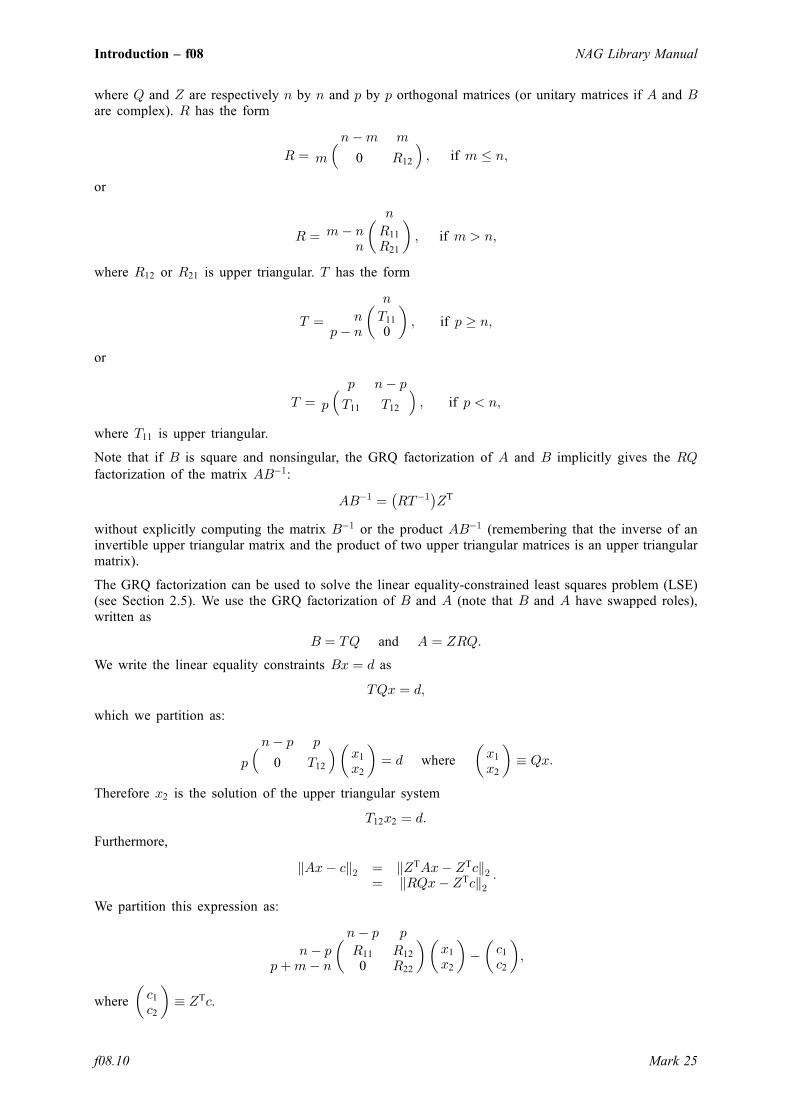
where Q and Z are respectively n by n and p by p orthogonal matrices (or unitary matrices if A and Bare complex). R has the form

R ¼��n�m m

m 0 R12 ; if m � n;

or

R ¼�� n

m� n R11

n R21; if m > n;

where R12 or R21 is upper triangular. T has the form

T ¼�� n

n T11

p� n 0; if p � n;

or

T ¼�� p n� p

p T11 T12 ; if p < n;

where T11 is upper triangular.

Note that if B is square and nonsingular, the GRQ factorization of A and B implicitly gives the RQfactorization of the matrix AB�1:

AB�1 ¼ RT�1� �

ZT

without explicitly computing the matrix B�1 or the product AB�1 (remembering that the inverse of aninvertible upper triangular matrix and the product of two upper triangular matrices is an upper triangularmatrix).

The GRQ factorization can be used to solve the linear equality-constrained least squares problem (LSE)(see Section 2.5). We use the GRQ factorization of B and A (note that B and A have swapped roles),written as

B ¼ TQ and A ¼ ZRQ:We write the linear equality constraints Bx ¼ d as

TQx ¼ d;

which we partition as:

��n� p p

p 0 T12x1

x2

� �¼ d where x1

x2

� �� Qx:

Therefore x2 is the solution of the upper triangular system

T12x2 ¼ d:Furthermore,

Ax� ck k2 ¼ ZTAx� ZTck k2¼ RQx� ZTck k2

:

We partition this expression as:

��n� p p

n� p R11 R12

pþm� n 0 R22

x1

x2

� �� c1

c2

� �;

where c1

c2

� �� ZTc.


f08.10 Mark 25

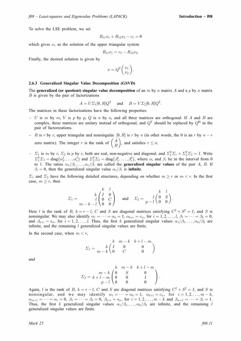
To solve the LSE problem, we set

R11x1 þR12x2 � c1 ¼ 0

which gives x1 as the solution of the upper triangular system

R11x1 ¼ c1 �R12x2:

Finally, the desired solution is given by

x ¼ QT x1

x2

� �:

2.6.3 Generalized Singular Value Decomposition (GSVD)

The generalized (or quotient) singular value decomposition of an m by n matrix A and a p by n matrixB is given by the pair of factorizations

A ¼ U�1 0; R½ QT and B ¼ V�2 0; R½ QT:

The matrices in these factorizations have the following properties:

– U is m by m, V is p by p, Q is n by n, and all three matrices are orthogonal. If A and B arecomplex, these matrices are unitary instead of orthogonal, and QT should be replaced by QH in thepair of factorizations.

– R is r by r, upper triangular and nonsingular. 0; R½ is r by n (in other words, the 0 is an r by n� r

zero matrix). The integer r is the rank of AB

� �, and satisfies r � n.

– �1 is m by r, �2 is p by r, both are real, non-negative and diagonal, and �T1�1 þ�T

2�2 ¼ I. Write

�T1�1 ¼ diag �2

1; . . . ; �2r

� �and �T

2�2 ¼ diag �21; . . . ; �2

r

� �, where �i and �i lie in the interval from 0

to 1. The ratios �1=�1; . . . ; �r=�r are called the generalized singular values of the pair A, B. If�i ¼ 0, then the generalized singular value �i=�i is infinite.

�1 and �2 have the following detailed structures, depending on whether m � r or m < r. In the firstcase, m � r, then

�1 ¼

1A

0@k l

k I 0l 0 C

m� k� l 0 0and �2 ¼

�� k l

l 0 Sp� l 0 0

:

Here l is the rank of B, k ¼ r� l, C and S are diagonal matrices satisfying C2 þ S2 ¼ I, and S isnonsingular. We may also identify �1 ¼ � � � ¼ �k ¼ 1, �kþi ¼ cii, for i ¼ 1; 2; . . . ; l, �1 ¼ � � � ¼ �k ¼ 0,and �kþi ¼ sii, for i ¼ 1; 2; . . . ; l. Thus, the first k generalized singular values �1=�1; . . . ; �k=�k areinfinite, and the remaining l generalized singular values are finite.

In the second case, when m < r,

�1 ¼�� k m� k kþ l�m

k I 0 0m� k 0 C 0

and

�2 ¼

1A

0@k m� k kþ l�m

m� k 0 S 0kþ l�m 0 0 I

p� l 0 0 0:

Again, l is the rank of B, k ¼ r� l, C and S are diagonal matrices satisfying C2 þ S2 ¼ I, and S isnonsingular, and we may identify �1 ¼ � � � ¼ �k ¼ 1, �kþi ¼ cii, for i ¼ 1; 2; . . . ;m� k,�mþ1 ¼ � � � ¼ �r ¼ 0, �1 ¼ � � � ¼ �k ¼ 0, �kþi ¼ sii, for i ¼ 1; 2; . . . ;m� k and �mþ1 ¼ � � � ¼ �r ¼ 1.Thus, the first k generalized singular values �1=�1; . . . ; �k=�k are infinite, and the remaining lgeneralized singular values are finite.


Mark 25 f08.11

Here are some important special cases of the generalized singular value decomposition. First, if B issquare and nonsingular, then r ¼ n and the generalized singular value decomposition of A and B isequivalent to the singular value decomposition of AB�1, where the singular values of AB�1 are equal tothe generalized singular values of the pair A, B:

AB�1 ¼ U�1RQT

� �V�2RQ

T� ��1 ¼ U �1�

�12

� �V T:

Second, for the matrix C, where

C � AB

� �

if the columns of C are orthonormal, then r ¼ n, R ¼ I and the generalized singular valuedecomposition of A and B is equivalent to the CS (Cosine–Sine) decomposition of C:

AB

� �¼ U 0

0 V

� ��1

�2

� �QT:

Third, the generalized eigenvalues and eigenvectors of ATA� �BTB can be expressed in terms of thegeneralized singular value decomposition: Let

X ¼ Q I 00 R�1

� �:

Then

XTATAX ¼ 0 00 �T

1�1

� �and XTBTBX ¼ 0 0

0 �T2�2

� �:

Therefore, the columns of X are the eigenvectors of ATA� �BTB, and ‘nontrivial’ eigenvalues are thesquares of the generalized singular values (see also Section 2.8). ‘Trivial’ eigenvalues are thosecorresponding to the leading n� r columns of X, which span the common null space of ATA and BTB.The ‘trivial eigenvalues’ are not well defined.

2.6.4 The Full CS Decomposition of Orthogonal Matrices

In Section 2.6.3 the CS (Cosine-Sine) decomposition of an orthogonal matrix partitioned into twosubmatrices A and B was given by

AB

� �¼ U 0

0 V

� ��1

�2

� �QT:

The full CS decomposition of an m by m orthogonal matrix X partitions X into four submatrices andfactorizes as

X11 X12

X21 X22

� �¼ U1 0

0 U2

� ��11 ��12

�21 �22

� �V1 00 V2

� �T

where, X11 is a p by q submatrix (which implies the dimensions of X12, X21 and X22); U1, U2, V1 andV2 are orthogonal matrices of dimensions p, m� p, q and m� q respectively; �11 is the p by q single-diagonal matrix

�11 ¼

1A

0@k11 � r r q � k11

k11 � r I 0 0r 0 C 0

p� k11 0 0; k11 ¼ min p; qð Þ

�12 is the p by m� q single-diagonal matrix

�12 ¼

1A

0@m� q � k12 r k12 � r

p� k12 0 0r 0 S 0

k12 � r 0 0 I

; k12 ¼ min p;m� qð Þ;

�21 is the m� p by q single-diagonal matrix


f08.12 Mark 25

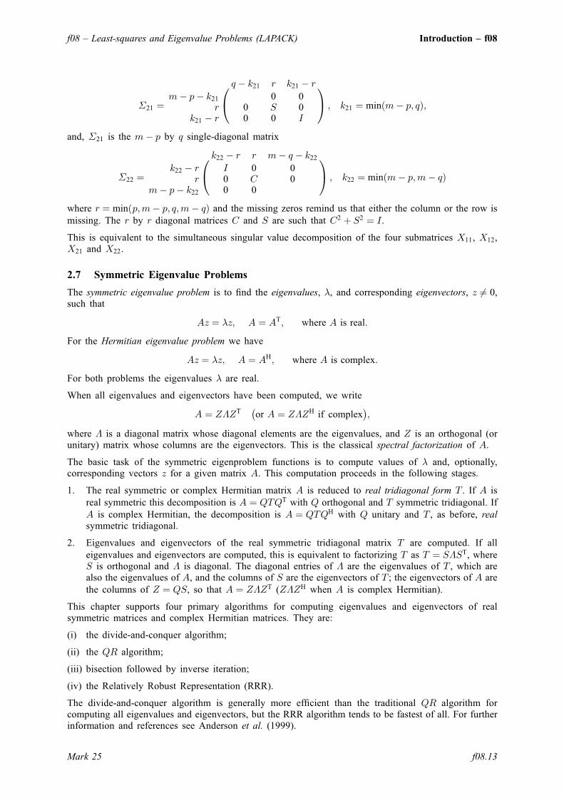
�21 ¼

1A

0@q � k21 r k21 � r

m� p� k21 0 0r 0 S 0

k21 � r 0 0 I

; k21 ¼ min m� p; qð Þ;

and, �21 is the m� p by q single-diagonal matrix

�22 ¼

1A

0@k22 � r r m� q � k22

k22 � r I 0 0r 0 C 0

m� p� k22 0 0; k22 ¼ min m� p;m� qð Þ

where r ¼ min p;m� p; q;m� qð Þ and the missing zeros remind us that either the column or the row ismissing. The r by r diagonal matrices C and S are such that C2 þ S2 ¼ I.

This is equivalent to the simultaneous singular value decomposition of the four submatrices X11, X12,X21 and X22.

2.7 Symmetric Eigenvalue Problems

The symmetric eigenvalue problem is to find the eigenvalues, �, and corresponding eigenvectors, z 6¼ 0,such that

Az ¼ �z; A ¼ AT; where A is real:

For the Hermitian eigenvalue problem we have

Az ¼ �z; A ¼ AH; where A is complex:

For both problems the eigenvalues � are real.

When all eigenvalues and eigenvectors have been computed, we write

A ¼ Z�ZT or A ¼ Z�ZH if complex� �

;

where � is a diagonal matrix whose diagonal elements are the eigenvalues, and Z is an orthogonal (orunitary) matrix whose columns are the eigenvectors. This is the classical spectral factorization of A.

The basic task of the symmetric eigenproblem functions is to compute values of � and, optionally,corresponding vectors z for a given matrix A. This computation proceeds in the following stages.

1. The real symmetric or complex Hermitian matrix A is reduced to real tridiagonal form T . If A isreal symmetric this decomposition is A ¼ QTQT with Q orthogonal and T symmetric tridiagonal. IfA is complex Hermitian, the decomposition is A ¼ QTQH with Q unitary and T , as before, realsymmetric tridiagonal.

2. Eigenvalues and eigenvectors of the real symmetric tridiagonal matrix T are computed. If alleigenvalues and eigenvectors are computed, this is equivalent to factorizing T as T ¼ S�ST, whereS is orthogonal and � is diagonal. The diagonal entries of � are the eigenvalues of T , which arealso the eigenvalues of A, and the columns of S are the eigenvectors of T ; the eigenvectors of A arethe columns of Z ¼ QS, so that A ¼ Z�ZT (Z�ZH when A is complex Hermitian).

This chapter supports four primary algorithms for computing eigenvalues and eigenvectors of realsymmetric matrices and complex Hermitian matrices. They are:

(i) the divide-and-conquer algorithm;

(ii) the QR algorithm;

(iii) bisection followed by inverse iteration;

(iv) the Relatively Robust Representation (RRR).

The divide-and-conquer algorithm is generally more efficient than the traditional QR algorithm forcomputing all eigenvalues and eigenvectors, but the RRR algorithm tends to be fastest of all. For furtherinformation and references see Anderson et al. (1999).


Mark 25 f08.13

2.8 Generalized Symmetric-definite Eigenvalue Problems

This section is concerned with the solution of the generalized eigenvalue problems Az ¼ �Bz,ABz ¼ �z, and BAz ¼ �z, where A and B are real symmetric or complex Hermitian and B is positivedefinite. Each of these problems can be reduced to a standard symmetric eigenvalue problem, using aCholesky factorization of B as either B ¼ LLT or B ¼ UTU (LLH or UHU in the Hermitian case).

With B ¼ LLT, we have

Az ¼ �Bz) L�1AL�T� �

LTz� �

¼ � LTz� �

:

Hence the eigenvalues of Az ¼ �Bz are those of Cy ¼ �y, where C is the symmetric matrixC ¼ L�1AL�T and y ¼ LTz. In the complex case C is Hermitian with C ¼ L�1AL�H and y ¼ LHz.

Table 1 summarises how each of the three types of problem may be reduced to standard form Cy ¼ �y,and how the eigenvectors z of the original problem may be recovered from the eigenvectors y of thereduced problem. The table applies to real problems; for complex problems, transposed matrices must bereplaced by conjugate-transposes.

Type of problem Factorization of B Reduction Recovery of eigenvectors

1. Az ¼ �Bz B ¼ LLT,B ¼ UTU

C ¼ L�1AL�T,C ¼ U�TAU�1

z ¼ L�Ty,z ¼ U�1y

2. ABz ¼ �z B ¼ LLT,B ¼ UTU

C ¼ LTAL,C ¼ UAUT

z ¼ L�Ty,z ¼ U�1y

3. BAz ¼ �z B ¼ LLT,B ¼ UTU

C ¼ LTAL,C ¼ UAUT

z ¼ Ly,z ¼ UTy

Table 1Reduction of generalized symmetric-definite eigenproblems to standard problems

When the generalized symmetric-definite problem has been reduced to the corresponding standardproblem Cy ¼ �y, this may then be solved using the functions described in the previous section. Nospecial functions are needed to recover the eigenvectors z of the generalized problem from theeigenvectors y of the standard problem, because these computations are simple applications of Level 2 orLevel 3 BLAS (see Chapter f16).

2.9 Packed Storage for Symmetric Matrices

Functions which handle symmetric matrices are usually designed so that they use either the upper orlower triangle of the matrix; it is not necessary to store the whole matrix. If either the upper or lowertriangle is stored conventionally in the upper or lower triangle of a two-dimensional array, the remainingelements of the array can be used to store other useful data. However, that is not always convenient, andif it is important to economize on storage, the upper or lower triangle can be stored in a one-dimensionalarray of length n nþ 1ð Þ=2; that is, the storage is almost halved.

This storage format is referred to as packed storage; it is described in Section 3.3.2 in the f07 ChapterIntroduction.

Functions designed for packed storage are usually less efficient, especially on high-performancecomputers, so there is a trade-off between storage and efficiency.

2.10 Band Matrices

A band matrix is one whose elements are confined to a relatively small number of subdiagonals orsuperdiagonals on either side of the main diagonal. Algorithms can take advantage of bandedness toreduce the amount of work and storage required. The storage scheme for band matrices is described inSection 3.3.4 in the f07 Chapter Introduction.


f08.14 Mark 25

If the problem is the generalized symmetric definite eigenvalue problem Az ¼ �Bz and the matrices Aand B are additionally banded, the matrix C as defined in Section 2.8 is, in general, full. We can reducethe problem to a banded standard problem by modifying the definition of C thus:

C ¼ XTAX; where X ¼ U�1Q or L�TQ;

where Q is an orthogonal matrix chosen to ensure that C has bandwidth no greater than that of A.

A further refinement is possible when A and B are banded, which halves the amount of work required toform C. Instead of the standard Cholesky factorization of B as UTU or LLT, we use a split Choleskyfactorization B ¼ STS, where

S ¼ U11

M21 L22

� �

with U11 upper triangular and L22 lower triangular of order approximately n=2; S has the samebandwidth as B.

2.11 Nonsymmetric Eigenvalue Problems

The nonsymmetric eigenvalue problem is to find the eigenvalues, �, and corresponding eigenvectors,v 6¼ 0, such that

Av ¼ �v:

More precisely, a vector v as just defined is called a right eigenvector of A, and a vector u 6¼ 0 satisfying

uTA ¼ �uT uHA ¼ �uH when u is complex� �

is called a left eigenvector of A.

A real matrix A may have complex eigenvalues, occurring as complex conjugate pairs.

This problem can be solved via the Schur factorization of A, defined in the real case as

A ¼ ZTZT;

where Z is an orthogonal matrix and T is an upper quasi-triangular matrix with 1 by 1 and 2 by 2diagonal blocks, the 2 by 2 blocks corresponding to complex conjugate pairs of eigenvalues of A. In thecomplex case, the Schur factorization is

A ¼ ZTZH;

where Z is unitary and T is a complex upper triangular matrix.

The columns of Z are called the Schur vectors. For each k (1 � k � n), the first k columns of Z form anorthonormal basis for the invariant subspace corresponding to the first k eigenvalues on the diagonal ofT . Because this basis is orthonormal, it is preferable in many applications to compute Schur vectorsrather than eigenvectors. It is possible to order the Schur factorization so that any desired set of keigenvalues occupy the k leading positions on the diagonal of T .

The two basic tasks of the nonsymmetric eigenvalue functions are to compute, for a given matrix A, alln values of � and, if desired, their associated right eigenvectors v and/or left eigenvectors u, and theSchur factorization.

These two basic tasks can be performed in the following stages.

1. A general matrix A is reduced to upper Hessenberg form H which is zero below the firstsubdiagonal. The reduction may be written A ¼ QHQT with Q orthogonal if A is real, orA ¼ QHQH with Q unitary if A is complex.

2. The upper Hessenberg matrix H is reduced to Schur form T , giving the Schur factorizationH ¼ STST (for H real) or H ¼ STSH (for H complex). The matrix S (the Schur vectors of H)may optionally be computed as well. Alternatively S may be postmultiplied into the matrix Qdetermined in stage 1, to give the matrix Z ¼ QS, the Schur vectors of A. The eigenvalues areobtained from the diagonal elements or diagonal blocks of T .


Mark 25 f08.15

3. Given the eigenvalues, the eigenvectors may be computed in two different ways. Inverse iterationcan be performed on H to compute the eigenvectors of H, and then the eigenvectors can bemultiplied by the matrix Q in order to transform them to eigenvectors of A. Alternatively theeigenvectors of T can be computed, and optionally transformed to those of H or A if the matrix Sor Z is supplied.

The accuracy with which eigenvalues can be obtained can often be improved by balancing a matrix. Thisis discussed further in Section 2.14.6 below.

2.12 Generalized Nonsymmetric Eigenvalue Problem

The generalized nonsymmetric eigenvalue problem is to find the eigenvalues, �, and correspondingeigenvectors, v 6¼ 0, such that

Av ¼ �Bv:More precisely, a vector v as just defined is called a right eigenvector of the matrix pair A;Bð Þ, and avector u 6¼ 0 satisfying

uTA ¼ �uTB uHA ¼ �uHB when u is complex� �

is called a left eigenvector of the matrix pair A;Bð Þ.If B is singular then the problem has one or more infinite eigenvalues � ¼ 1, corresponding to Bv ¼ 0.Note that if A is nonsingular, then the equivalent problem �Av ¼ Bv is perfectly well defined and aninfinite eigenvalue corresponds to � ¼ 0. To deal with both finite (including zero) and infiniteeigenvalues, the functions in this chapter do not compute � explicitly, but rather return a pair of numbers�; �ð Þ such that if � 6¼ 0

� ¼ �=�

and if � 6¼ 0 and � ¼ 0 then � ¼ 1. � is always returned as real and non-negative. Of course,computationally an infinite eigenvalue may correspond to a small � rather than an exact zero.

For a given pair A;Bð Þ the set of all the matrices of the form A� �Bð Þ is called a matrix pencil and �and v are said to be an eigenvalue and eigenvector of the pencil A� �Bð Þ. If A and B are both singularand share a common null space then

det A� �Bð Þ � 0

so that the pencil A� �Bð Þ is singular for all �. In other words any � can be regarded as an eigenvalue.In exact arithmetic a singular pencil will have � ¼ � ¼ 0 for some �; �ð Þ. Computationally if some pair�; �ð Þ is small then the pencil is singular, or nearly singular, and no reliance can be placed on any of the

computed eigenvalues. Singular pencils can also manifest themselves in other ways; see, in particular,Sections 2.3.5.2 and 4.11.1.4 of Anderson et al. (1999) for further details.

The generalized eigenvalue problem can be solved via the generalized Schur factorization of the pairA;Bð Þ defined in the real case as

A ¼ QSZT; B ¼ QTZT;

where Q and Z are orthogonal, T is upper triangular with non-negative diagonal elements and S is upperquasi-triangular with 1 by 1 and 2 by 2 diagonal blocks, the 2 by 2 blocks corresponding to complexconjugate pairs of eigenvalues. In the complex case, the generalized Schur factorization is

A ¼ QSZH; B ¼ QTZH;

where Q and Z are unitary and S and T are upper triangular, with T having real non-negative diagonalelements. The columns of Q and Z are called respectively the left and right generalized Schur vectorsand span pairs of deflating subspaces of A and B, which are a generalization of invariant subspaces.

It is possible to order the generalized Schur factorization so that any desired set of k eigenvaluescorrespond to the k leading positions on the diagonals of the pair S; Tð Þ.


f08.16 Mark 25

The two basic tasks of the generalized nonsymmetric eigenvalue functions are to compute, for a givenpair A;Bð Þ, all n values of � and, if desired, their associated right eigenvectors v and/or left eigenvectorsu, and the generalized Schur factorization.

These two basic tasks can be performed in the following stages.

1. The matrix pair A;Bð Þ is reduced to generalized upper Hessenberg form H;Rð Þ, where H is upperHessenberg (zero below the first subdiagonal) and R is upper triangular. The reduction may bewritten as A ¼ Q1HZ

T1 ; B ¼ Q1RZ

T1 in the real case with Q1 and Z1 orthogonal, and

A ¼ Q1HZH1 ; B ¼ Q1RZ

H1 in the complex case with Q1 and Z1 unitary.

2. The generalized upper Hessenberg form H;Rð Þ is reduced to the generalized Schur form S; Tð Þusing the generalized Schur factorization H ¼ Q2SZ

T2 , R ¼ Q2TZ

T2 in the real case with Q2 and Z2

orthogonal, and H ¼ Q2SZH2 ; R ¼ Q2TZ

H2 in the complex case. The generalized Schur vectors of

A;Bð Þ are given by Q ¼ Q1Q2, Z ¼ Z1Z2. The eigenvalues are obtained from the diagonalelements (or blocks) of the pair S; Tð Þ.

3. Given the eigenvalues, the eigenvectors of the pair S; Tð Þ can be computed, and optionallytransformed to those of H;Rð Þ or A;Bð Þ.

The accuracy with which eigenvalues can be obtained can often be improved by balancing a matrix pair.This is discussed further in Section 2.14.8 below.

2.13 The Sylvester Equation and the Generalized Sylvester Equation

The Sylvester equation is a matrix equation of the form

AX þXB ¼ C;

where A, B, and C are given matrices with A being m by m, B an n by n matrix and C, and thesolution matrix X, m by n matrices. The solution of a special case of this equation occurs in thecomputation of the condition number for an invariant subspace, but a combination of functions in thischapter allows the solution of the general Sylvester equation.

Functions are also provided for solving a special case of the generalized Sylvester equations

AR� LB ¼ C; DR� LE ¼ F;

where A;Dð Þ, B;Eð Þ and C; Fð Þ are given matrix pairs, and R and L are the solution matrices.

2.14 Error and Perturbation Bounds and Condition Numbers

In this section we discuss the effects of rounding errors in the solution process and the effects ofuncertainties in the data, on the solution to the problem. A number of the functions in this chapter returninformation, such as condition numbers, that allow these effects to be assessed. First we discuss somenotation used in the error bounds of later sections.

The bounds usually contain the factor p nð Þ (or p m; nð Þ), which grows as a function of the matrixdimension n (or matrix dimensions m and n). It measures how errors can grow as a function of thematrix dimension, and represents a potentially different function for each problem. In practice, it usuallygrows just linearly; p nð Þ � 10n is often true, although generally only much weaker bounds can beactually proved. We normally describe p nð Þ as a ‘modestly growing’ function of n. For detailedderivations of various p nð Þ, see Golub and Van Loan (2012) and Wilkinson (1965).

For linear equation (see Chapter f07) and least squares solvers, we consider bounds on the relative errorx� xk k= xk k in the computed solution x, where x is the true solution. For eigenvalue problems we

consider bounds on the error �i � �i in the ith computed eigenvalue �i, where �i is the true ith

eigenvalue. For singular value problems we similarly consider bounds �i � �ij j.Bounding the error in computed eigenvectors and singular vectors vi is more subtle because thesevectors are not unique: even though we restrict vik k2 ¼ 1 and vik k2 ¼ 1, we may still multiply them byarbitrary constants of absolute value 1. So to avoid ambiguity we bound the angular difference betweenvi and the true vector vi, so that


Mark 25 f08.17

vi; við Þ ¼ acute angle between vi and vi¼ arccos vH

i vi : ð2Þ

Here arccos ð Þ is in the standard range: 0 � arccos ð Þ < . When vi; við Þ is small, we can choose aconstant � with absolute value 1 so that �vi � vik k2 vi; við Þ.In addition to bounds for individual eigenvectors, bounds can be obtained for the spaces spanned bycollections of eigenvectors. These may be much more accurately determined than the individualeigenvectors which span them. These spaces are called invariant subspaces in the case of eigenvectors,because if v is any vector in the space, Av is also in the space, where A is the matrix. Again, we will use

angle to measure the difference between a computed space S and the true space S:

S; S� �

¼ acute angle between S and S

¼ maxs2Ss6¼0

mins2Ss6¼0

s; sð Þ or maxs2Ss6¼0

mins2Ss6¼0

s; sð Þ ð3Þ

S; S� �

may be computed as follows. Let S be a matrix whose columns are orthonormal and spanS.

Similarly let S be an orthonormal matrix with columns spanning S. Then

S; S� �

¼ arccos�min SHS� �

:

Finally, we remark on the accuracy of the bounds when they are large. Relative errors like x� xk k= xk kand angular errors like vi; við Þ are only of interest when they are much less than 1. Some stated boundsare not strictly true when they are close to 1, but rigorous bounds are much more complicated andsupply little extra information in the interesting case of small errors. These bounds are indicated by usingthe symbol �< , or ‘approximately less than’, instead of the usual �. Thus, when these bounds are closeto 1 or greater, they indicate that the computed answer may have no significant digits at all, but do nototherwise bound the error.

A number of functions in this chapter return error estimates and/or condition number estimates directly.In other cases Anderson et al. (1999) gives code fragments to illustrate the computation of theseestimates, and a number of the Chapter f08 example programs, for the driver functions, implement thesecode fragments.

2.14.1 Least squares problems

The conventional error analysis of linear least squares problems goes as follows. The problem is to findthe x minimizing Ax� bk k2. Let x be the solution computed using one of the methods described above.We discuss the most common case, where A is overdetermined (i.e., has more rows than columns) andhas full rank.

Then the computed solution x has a small normwise backward error. In other words x minimizesAþ Eð Þx� bþ fð Þk k2, where

maxEk k2

Ak k2

;fk k2

bk k2

� �� p nð Þ�

and p nð Þ is a modestly growing function of n and � is the machine precision. Let�2 Að Þ ¼ �max Að Þ=�min Að Þ, ¼ Ax� bk k2, and sin ð Þ ¼ = bk k2. Then if p nð Þ� is small enough, theerror x� x is bounded by

x� xk k2

xk k2�< p nð Þ� 2�2 Að Þ

cos ð Þ þ tan ð Þ�22 Að Þ

�:

If A is rank-deficient, the problem can be regularized by treating all singular values less than a user-specified threshold as exactly zero. See Golub and Van Loan (2012) for error bounds in this case, as wellas for the underdetermined case.

The solution of the overdetermined, full-rank problem may also be characterised as the solution of thelinear system of equations


f08.18 Mark 25

I AAT 0

� �rx

� �¼ b

0

� �:

By solving this linear system (see Chapter f07) component-wise error bounds can also be obtained (seeArioli et al. (1989)).

2.14.2 The singular value decomposition

The usual error analysis of the SVD algorithm is as follows (see Golub and Van Loan (2012)).

The computed SVD, U�V T, is nearly the exact SVD of Aþ E, i.e., Aþ E ¼ U þ �U� �

� V þ �V� �

is

the true SVD, so that U þ �U and V þ �V are both orthogonal, where Ek k2= Ak k2 � p m; nð Þ�,�U�� p m; nð Þ�, and �V

�� p m; nð Þ�. Here p m; nð Þ is a modestly growing function of m and n and �is the machine precision. Each computed singular value �i differs from the true �i by an amountsatisfying the bound

�i � �ij j � p m; nð Þ��1:

Thus large singular values (those near �1) are computed to high relative accuracy and small ones maynot be.

The angular difference between the computed left singular vector ui and the true ui satisfies theapproximate bound

ui; uið Þ �<p m; nð Þ� Ak k2

gapi

where

gapi ¼ minj6¼i

�i � �j

is the absolute gap between �i and the nearest other singular value. Thus, if �i is close to other singularvalues, its corresponding singular vector ui may be inaccurate. The same bound applies to the computedright singular vector vi and the true vector vi. The gaps may be easily obtained from the computedsingular values.

Let S be the space spanned by a collection of computed left singular vectors ui; i 2 If g, where I is asubset of the integers from 1 to n. Let S be the corresponding true space. Then

S; S� �

�<p m; nð Þ� Ak k2

gapI

:

where

gapI ¼ min �i � �j for i 2 I ; j =2 I�

is the absolute gap between the singular values in I and the nearest other singular value. Thus, a clusterof close singular values which is far away from any other singular value may have a well determined

space S even if its individual singular vectors are ill-conditioned. The same bound applies to a set ofright singular vectors vi; i 2 If g.In the special case of bidiagonal matrices, the singular values and singular vectors may be computedmuch more accurately (see Demmel and Kahan (1990)). A bidiagonal matrix B has nonzero entries onlyon the main diagonal and the diagonal immediately above it (or immediately below it). Reduction of adense matrix to bidiagonal form B can introduce additional errors, so the following bounds for thebidiagonal case do not apply to the dense case.

Using the functions in this chapter, each computed singular value of a bidiagonal matrix is accurate tonearly full relative accuracy, no matter how tiny it is, so that

�i � �ij j � p m; nð Þ��i:


Mark 25 f08.19

The computed left singular vector ui has an angular error at most about

ui; uið Þ �<p m; nð Þ�relgapi

where

relgapi ¼ minj6¼i

�i � �j = �i þ �j� �

is the relative gap between �i and the nearest other singular value. The same bound applies to the rightsingular vector vi and vi. Since the relative gap may be much larger than the absolute gap, this errorbound may be much smaller than the previous one. The relative gaps may be easily obtained from thecomputed singular values.

2.14.3 The symmetric eigenproblem

The usual error analysis of the symmetric eigenproblem is as follows (see Parlett (1998)).

The computed eigendecomposition Z�ZT is nearly the exact eigendecomposition of Aþ E, i.e.,

Aþ E ¼ Z þ �Z� �

� Z þ �Z� �T

is the true eigendecomposition so that Z þ �Z is orthogonal, where

Ek k2= Ak k2 � p nð Þ� and �Z��

2� p nð Þ� and p nð Þ is a modestly growing function of n and � is the

machine precision. Each computed eigenvalue �i differs from the true �i by an amount satisfying thebound

�i � �i � p nð Þ� Ak k2:

Thus large eigenvalues (those near maxi�ij j ¼ Ak k2) are computed to high relative accuracy and small

ones may not be.

The angular difference between the computed unit eigenvector zi and the true zi satisfies the approximatebound

zi; zið Þ �<p nð Þ� Ak k2

gapi

if p nð Þ� is small enough, where

gapi ¼ minj6¼i

�i � �j

is the absolute gap between �i and the nearest other eigenvalue. Thus, if �i is close to other eigenvalues,its corresponding eigenvector zi may be inaccurate. The gaps may be easily obtained from the computedeigenvalues.

Let S be the invariant subspace spanned by a collection of eigenvectors zi; i 2 If g, where I is a subsetof the integers from 1 to n. Let S be the corresponding true subspace. Then

S; S� �

�<p nð Þ� Ak k2

gapI

where

gapI ¼ min �i � �j for i 2 I ; j =2 I�

is the absolute gap between the eigenvalues in I and the nearest other eigenvalue. Thus, a cluster ofclose eigenvalues which is far away from any other eigenvalue may have a well determined invariant

subspace S even if its individual eigenvectors are ill-conditioned.

In the special case of a real symmetric tridiagonal matrix T , functions in this chapter can compute theeigenvalues and eigenvectors much more accurately. See Anderson et al. (1999) for further details.


f08.20 Mark 25

2.14.4 The generalized symmetric-definite eigenproblem

The three types of problem to be considered are A� �B, AB� �I and BA� �I. In each case A and Bare real symmetric (or complex Hermitian) and B is positive definite. We consider each case in turn,assuming that functions in this chapter are used to transform the generalized problem to the standardsymmetric problem, followed by the solution of the symmetric problem. In all cases

gapi ¼ minj6¼i

�i � �j

is the absolute gap between �i and the nearest other eigenvalue.

1. A� �B. The computed eigenvalues �i can differ from the true eigenvalues �i by an amount

�i � �i �< p nð Þ� B�1

�� 2Ak k2:

The angular difference between the computed eigenvector zi and the true eigenvector zi is

zi; zið Þ �<p nð Þ� B�1

�� 2Ak k2 �2 Bð Þð Þ1=2

gapi:

2. AB� �I or BA� �I. The computed eigenvalues �i can differ from the true eigenvalues �i by anamount

�i � �i �< p nð Þ� Bk k2 Ak k2:

The angular difference between the computed eigenvector zi and the true eigenvector zi is

zi; zið Þ �<p nð Þ� Bk k2 Ak k2 �2 Bð Þð Þ1=2

gapi:

These error bounds are large when B is ill-conditioned with respect to inversion (�2 Bð Þ is large). It isoften the case that the eigenvalues and eigenvectors are much better conditioned than indicated here.One way to get tighter bounds is effective when the diagonal entries of B differ widely in magnitude, asfor example with a graded matrix.

1. A� �B. Let D ¼ diag b�1=211 ; . . . ; b�1=2

nn

� �be a diagonal matrix. Then replace B by DBD and A by

DAD in the above bounds.

2. AB� �I or BA� �I. Let D ¼ diag b�1=211 ; . . . ; b�1=2

nn

� �be a diagonal matrix. Then replace B by

DBD and A by D�1AD�1 in the above bounds.

Further details can be found in Anderson et al. (1999).

2.14.5 The nonsymmetric eigenproblem

The nonsymmetric eigenvalue problem is more complicated than the symmetric eigenvalue problem. Inthis section, we just summarise the bounds. Further details can be found in Anderson et al. (1999).

We let �i be the ith computed eigenvalue and �i the ith true eigenvalue. Let vi be the correspondingcomputed right eigenvector, and vi the true right eigenvector (so Avi ¼ �ivi). If I is a subset of the

integers from 1 to n, we let �I denote the average of the selected eigenvalues: �I ¼Pi2I�i

� �=Pi2I

1

� �,

and similarly for �I. We also let SI denote the subspace spanned by vi; i 2 If g; it is called a right

invariant subspace because if v is any vector in SI then Av is also in SI . SI is the correspondingcomputed subspace.

The algorithms for the nonsymmetric eigenproblem are normwise backward stable: they compute theexact eigenvalues, eigenvectors and invariant subspaces of slightly perturbed matrices Aþ Eð Þ, whereEk k � p nð Þ� Ak k. Some of the bounds are stated in terms of Ek k2 and others in terms of Ek kF ; one may

use p nð Þ� for either quantity.


Mark 25 f08.21

Functions are provided so that, for each (�i; vi) pair the two values si and sepi, or for a selected subset Iof eigenvalues the values sI and sepI can be obtained, for which the error bounds in Table 2 are true forsufficiently small Ek k, (which is why they are called asymptotic):

Simple eigenvalue �i � �i �< Ek k2=si

Eigenvalue cluster �I � �I

�< Ek k2=sI

Eigenvector vi; við Þ �< Ek kF=sepi

Invariant subspace SI ; SI

� ��< Ek kF=sepI

Table 2Asymptotic error bounds for the nonsymmetric

eigenproblem

If the problem is ill-conditioned, the asymptotic bounds may only hold for extremely small Ek k. Theglobal error bounds of Table 3 are guaranteed to hold for all Ek kF < s� sep=4:

Simpleeigenvalue

�i � �i � n Ek k2=si Holds for all E

Eigenvaluecluster

�I � �I

� 2 Ek k2=sI Requires Ek kF < sI � sepI=4

Eigenvector vi; við Þ � arctan 2 Ek kF= sepi � 4 Ek kF=si� ��

Requires Ek kF < si � sepi=4

Invariantsubspace

SI ; SI

� �� arctan 2 Ek kF= sepI � 4 Ek kF=sI

� �� Requires Ek kF < sI � sepI=4

Table 3Global error bounds for the nonsymmetric eigenproblem

2.14.6 Balancing and condition for the nonsymmetric eigenproblem

There are two preprocessing steps one may perform on a matrix A in order to make its eigenproblemeasier. The first is permutation, or reordering the rows and columns to make A more nearly uppertriangular (closer to Schur form): A0 ¼ PAP T, where P is a permutation matrix. If A0 is permutable toupper triangular form (or close to it), then no floating-point operations (or very few) are needed toreduce it to Schur form. The second is scaling by a diagonal matrix D to make the rows and columns ofA0 more nearly equal in norm: A00 ¼ DA0D�1. Scaling can make the matrix norm smaller with respect tothe eigenvalues, and so possibly reduce the inaccuracy contributed by roundoff (see Chapter 11 ofWilkinson and Reinsch (1971)). We refer to these two operations as balancing.

Permuting has no effect on the condition numbers or their interpretation as described previously. Scaling,however, does change their interpretation and further details can be found in Anderson et al. (1999).

2.14.7 The generalized nonsymmetric eigenvalue problem

The algorithms for the generalized nonsymmetric eigenvalue problem are normwise backward stable:they compute the exact eigenvalues (as the pairs �; �ð Þ), eigenvectors and deflating subspaces of slightlyperturbed pairs Aþ E;Bþ Fð Þ, where

E;Fð Þk kF � p nð Þ� A;Bð Þk kF :Asymptotic and global error bounds can be obtained, which are generalizations of those given inTables 2 and 3. See Section 4.11 of Anderson et al. (1999) for details. Functions are provided tocompute estimates of reciprocal conditions numbers for eigenvalues and eigenspaces.


f08.22 Mark 25

2.14.8 Balancing the generalized eigenvalue problem

As with the standard nonsymmetric eigenvalue problem, there are two preprocessing steps one mayperform on a matrix pair A;Bð Þ in order to make its eigenproblem easier; permutation and scaling,which together are referred to as balancing, as indicated in the following two steps.

1. The balancing function first attempts to permute A and B to block upper triangular form by asimilarity transformation:

PAP T ¼ F ¼F11 F12 F13

F22 F23

F33

0@

1A;

PBPT ¼ G ¼G11 G12 G13

G22 G23

G33

0@

1A;

where P is a permutation matrix, F11, F33, G11 and G33 are upper triangular. Then the diagonalelements of the matrix F11; G11ð Þ and G33; H33ð Þ are generalized eigenvalues of A;Bð Þ. The rest ofthe generalized eigenvalues are given by the matrix pair F22; G22ð Þ. Subsequent operations tocompute the eigenvalues of A;Bð Þ need only be applied to the matrix F22; G22ð Þ; this can save asignificant amount of work if F22; G22ð Þ is smaller than the original matrix pair A;Bð Þ. If no suitablepermutation exists (as is often the case), then there is no gain in efficiency or accuracy.

2. The balancing function applies a diagonal similarity transformation to F;Gð Þ, to make the rows andcolumns of F22; G22ð Þ as close as possible in the norm:

DFD�1 ¼I

D22

I

0@

1A F11 F12 F13

F22 F23

F33

0@

1A I

D�122

I

0@

1A;

DGD�1 ¼I

D22

I

0@

1A G11 G12 G13

G22 G23

G33

0@

1A I

D�122

I

0@

1A:

This transformation usually improves the accuracy of computed generalized eigenvalues andeigenvectors. However, there are exceptional occasions when this transformation increases the normof the pencil; in this case accuracy could be lower with diagonal balancing.

See Anderson et al. (1999) for further details.

2.14.9 Other problems

Error bounds for other problems such as the generalized linear least squares problem and generalizedsingular value decomposition can be found in Anderson et al. (1999).

2.15 Block Partitioned Algorithms

A number of the functions in this chapter use what is termed a block partitioned algorithm. This meansthat at each major step of the algorithm a block of rows or columns is updated, and much of thecomputation is performed by matrix-matrix operations on these blocks. The matrix-matrix operations areperformed by calls to the Level 3 BLAS (see Chapter f16), which are the key to achieving highperformance on many modern computers. In the case of the QR algorithm for reducing an upperHessenberg matrix to Schur form, a multishift strategy is used in order to improve performance. SeeGolub and Van Loan (2012) or Anderson et al. (1999) for more about block partitioned algorithms andthe multishift strategy.

The performance of a block partitioned algorithm varies to some extent with the block size – that is, thenumber of rows or columns per block. This is a machine-dependent argument, which is set to a suitablevalue when the library is implemented on each range of machines. You do not normally need to be


Mark 25 f08.23

aware of what value is being used. Different block sizes may be used for different functions. Values inthe range 16 to 64 are typical.

On more conventional machines there is often no advantage from using a block partitioned algorithm,and then the functions use an unblocked algorithm (effectively a block size of 1), relying solely on callsto the Level 2 BLAS (see Chapter f16 again).

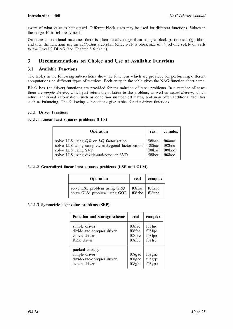
3 Recommendations on Choice and Use of Available Functions

3.1 Available Functions

The tables in the following sub-sections show the functions which are provided for performing differentcomputations on different types of matrices. Each entry in the table gives the NAG function short name.

Black box (or driver) functions are provided for the solution of most problems. In a number of casesthere are simple drivers, which just return the solution to the problem, as well as expert drivers, whichreturn additional information, such as condition number estimates, and may offer additional facilitiessuch as balancing. The following sub-sections give tables for the driver functions.

3.1.1 Driver functions

3.1.1.1 Linear least squares problems (LLS)

Operation real complex

solve LLS using QR or LQ factorizationsolve LLS using complete orthogonal factorizationsolve LLS using SVDsolve LLS using divide-and-conquer SVD

f08aacf08bacf08kacf08kcc

f08ancf08bncf08kncf08kqc

3.1.1.2 Generalized linear least squares problems (LSE and GLM)

Operation real complex

solve LSE problem using GRQsolve GLM problem using GQR

f08zacf08zbc

f08zncf08zpc

3.1.1.3 Symmetric eigenvalue problems (SEP)

Function and storage scheme real complex

simple driverdivide-and-conquer driverexpert driverRRR driver

f08facf08fccf08fbcf08fdc

f08fncf08fqcf08fpcf08frc

packed storagesimple driverdivide-and-conquer driverexpert driver

f08gacf08gccf08gbc

f08gncf08gqcf08gpc


f08.24 Mark 25

band matrixsimple driverdivide-and-conquer driverexpert driver

f08hacf08hccf08hbc

f08hncf08hqcf08hpc

tridiagonal matrixsimple driverdivide-and-conquer driverexpert driverRRR driver

f08jacf08jccf08jbcf08jdc

3.1.1.4 Nonsymmetric eigenvalue problem (NEP)


simple driver for Schur factorizationexpert driver for Schur factorizationsimple driver for eigenvalues/vectorsexpert driver for eigenvalues/vectors

f08pacf08pbcf08nacf08nbc

f08pncf08ppcf08nncf08npc

3.1.1.5 Singular value decomposition (SVD)


simple driverdivide-and-conquer driversimple driver for one-sided Jacobi SVDexpert driver for one-sided Jacobi SVD

f08kbcf08kdcf08kjcf08khc

f08kpcf08krc

3.1.1.6 Generalized symmetric definite eigenvalue problems (GSEP)


simple driverdivide-and-conquer driverexpert driver

f08sacf08sccf08sbc

f08sncf08sqcf08spc

packed storagesimple driverdivide-and-conquer driverexpert driver

f08tacf08tccf08tbc

f08tncf08tqcf08tpc

band matrixsimple driverdivide-and-conquer driverexpert driver

f08uacf08uccf08ubc

f08uncf08uqcf08upc


Mark 25 f08.25

3.1.1.7 Generalized nonsymmetric eigenvalue problem (GNEP)


simple driver for Schur factorizationexpert driver for Schur factorizationsimple driver for eigenvalues/vectorsexpert driver for eigenvalues/vectors

f08xacf08xbcf08wacf08wbc

f08xncf08xpcf08wncf08wpc

3.1.1.8 Generalized singular value decomposition (GSVD)


singular values/vectors f08vac f08vnc

3.1.2 Computational functions

It is possible to solve problems by calling two or more functions in sequence. Some common sequencesof functions are indicated in the tables in the following sub-sections; an asterisk ( ) against a functionname means that the sequence of calls is illustrated in the example program for that function.

3.1.2.1 Orthogonal factorizations

Functions are provided for QR factorization (with and without column pivoting), and for LQ, QL andRQ factorizations (without pivoting only), of a general real or complex rectangular matrix. A function isalso provided for the RQ factorization of a real or complex upper trapezoidal matrix. (LAPACK refers tothis as the RZ factorization.)

The factorization functions do not form the matrix Q explicitly, but represent it as a product ofelementary reflectors (see Section 3.3.6). Additional functions are provided to generate all or part of Qexplicitly if it is required, or to apply Q in its factored form to another matrix (specifically to computeone of the matrix products QC, QTC, CQ or CQT with QT replaced by QH if C and Q are complex).

Factorizewithoutpivoting

Factorizewithpivoting

Factorize(blocked)

Generatematrix Q

Applymatrix Q

ApplyQ (blocked)

QR factorization,real matrices

f08aec f08bfc f08abc f08afc f08agc f08acc

QR factorization,real triangular-pentagonal

f08bbc f08bcc

LQ factorization,real matrices

f08ahc f08ajc f08akc

QL factorization,real matrices

f08cec f08cfc f08cgc

RQ factorization,real matrices

f08chc f08cjc f08ckc

RQ factorization,real upper trapezoidal matrices

f08bhc f08bkc

QR factorization,complex matrices

f08asc f08btc f08apc f08atc f08auc f08aqc

QR factorization,complex triangular-pentagonal

f08bpc f08bqc

LQ factorization,complex matrices

f08avc f08awc f08axc

QL factorization,complex matrices

f08csc f08ctc f08cuc


f08.26 Mark 25

RQ factorization,complex matrices

f08cvc f08cwc f08cxc

RQ factorization,complex upper trapezoidal matrices

f08bvc f08bxc

To solve linear least squares problems, as described in Sections 2.2.1 or 2.2.3, functions based on theQR factorization can be used:

real data, full-rank problem f08aac, f08aec and f08agc,f08abc and f08acc, f16yjc

complex data, full-rank problem f08anc, f08asc and f08auc,f08apc and f08aqc, f16zjc

real data, rank-deficient problem f08bfc*, f16yjc, f08agccomplex data, rank-deficient problem f08btc*, f16zjc, f08auc

To find the minimum norm solution of under-determined systems of linear equations, as described inSection 2.2.2, functions based on the LQ factorization can be used:

real data, full-rank problem f08ahc*, f16yjc, f08akccomplex data, full-rank problem f08avc*, f16zjc, f08axc

3.1.2.2 Generalized orthogonal factorizations

Functions are provided for the generalized QR and RQ factorizations of real and complex matrix pairs.

Factorize

Generalized QR factorization, real matrices f08zec

Generalized RQ factorization, real matrices f08zfc

Generalized QR factorization, complex matrices f08zsc

Generalized RQ factorization, complex matrices f08ztc

3.1.2.3 Singular value problems

Functions are provided to reduce a general real or complex rectangular matrix A to real bidiagonal formB by an orthogonal transformation A ¼ QBPT (or by a unitary transformation A ¼ QBPH if A iscomplex). Different functions allow a full matrix A to be stored conventionally (see Section 3.3.1), or aband matrix to use band storage (see Section 3.3.4 in the f07 Chapter Introduction).

The functions for reducing full matrices do not form the matrix Q or P explicitly; additional functionsare provided to generate all or part of them, or to apply them to another matrix, as with the functions fororthogonal factorizations. Explicit generation of Q or P is required before using the bidiagonal QRalgorithm to compute left or right singular vectors of A.

The functions for reducing band matrices have options to generate Q or P if required.

Further functions are provided to compute all or part of the singular value decomposition of a realbidiagonal matrix; the same functions can be used to compute the singular value decomposition of a realor complex matrix that has been reduced to bidiagonal form.

Reduce tobidiagonalform

Generatematrix Q

or PT

Applymatrix Qor P

Reduce bandmatrix tobidiagonalform

SVD ofbidiagonalform (QRalgorithm)

SVD ofbidiagonalform (divide andconquer)

real matrices f08kec f08kfc f08kgc f08lec f08mec f08mdc

complex matrices f08ksc f08ktc f08kuc f08lsc f08msc


Mark 25 f08.27

Given the singular values, f08flc is provided to compute the reciprocal condition numbers for the left orright singular vectors of a real or complex matrix.

To compute the singular values and vectors of a rectangular matrix, as described in Section 2.3, use thefollowing sequence of calls:

Rectangular matrix (standard storage)

real matrix, singular values and vectors f08kec, f08kfc*, f08meccomplex matrix, singular values and vectors f08ksc, f08ktc*, f08msc

Rectangular matrix (banded)

real matrix, singular values and vectors f08lec, f08kfc, f08meccomplex matrix, singular values and vectors f08lsc, f08ktc, f08msc

To use the singular value decomposition to solve a linear least squares problem, as described inSection 2.4, the following functions are required:

real data f16yac, f08kec, f08kfc,f08kgc, f08mec

complex data f16zac, f08ksc, f08ktc,f08kuc, f08msc

3.1.2.4 Generalized singular value decomposition

Functions are provided to compute the generalized SVD of a real or complex matrix pair A;Bð Þ in uppertrapezoidal form. Functions are also provided to reduce a general real or complex matrix pair to therequired upper trapezoidal form.

Reduce totrapezoidal form

Generalized SVDof trapezoidal form

real matrices f08vec f08yec

complex matrices f08vsc f08ysc

Functions are provided for the full CS decomposition of orthogonal and unitary matrices expressed as 2by 2 partitions of submatrices. For real orthogonal matrices the CS decomposition is performed byf08rac, while for unitary matrices the equivalent function is f08rnc.

3.1.2.5 Symmetric eigenvalue problems

Functions are provided to reduce a real symmetric or complex Hermitian matrix A to real tridiagonalform T by an orthogonal similarity transformation A ¼ QTQT (or by a unitary transformationA ¼ QTQH if A is complex). Different functions allow a full matrix A to be stored conventionally (seeSection 3.3.1 in the f07 Chapter Introduction) or in packed storage (see Section 3.3.2 in the f07 ChapterIntroduction); or a band matrix to use band storage (see Section 3.3.4 in the f07 Chapter Introduction).

The functions for reducing full matrices do not form the matrix Q explicitly; additional functions areprovided to generate Q, or to apply it to another matrix, as with the functions for orthogonalfactorizations. Explicit generation of Q is required before using the QR algorithm to find all theeigenvectors of A; application of Q to another matrix is required after eigenvectors of T have beenfound by inverse iteration, in order to transform them to eigenvectors of A.

The functions for reducing band matrices have an option to generate Q if required.


f08.28 Mark 25

Reduce totridiagonalform

Generatematrix Q

Applymatrix Q

real symmetric matrices f08fec f08ffc f08fgc

real symmetric matrices (packed storage) f08gec f08gfc f08ggc

real symmetric band matrices f08hec

complex Hermitianmatrices

f08fsc f08ftc f08fuc

complex Hermitian matrices (packed storage) f08gsc f08gtc f08guc

complex Hermitian band matrices f08hsc

Given the eigenvalues, f08flc is provided to compute the reciprocal condition numbers for theeigenvectors of a real symmetric or complex Hermitian matrix.

A variety of functions are provided to compute eigenvalues and eigenvectors of the real symmetrictridiagonal matrix T , some computing all eigenvalues and eigenvectors, some computing selectedeigenvalues and eigenvectors. The same functions can be used to compute eigenvalues and eigenvectorsof a real symmetric or complex Hermitian matrix which has been reduced to tridiagonal form.

Eigenvalues and eigenvectors of real symmetric tridiagonal matrices:

The original (non-reduced) matrix is Real Symmetric or Complex Hermitian

all eigenvalues (root-free QR algorithm) f08jfcall eigenvalues (root-free QR algorithm called by divide-and-conquer) f08jcc or f08jhcall eigenvalues (RRR) f08jlcselected eigenvalues (bisection) f08jjc

The original (non-reduced) matrix is Real Symmetric

all eigenvalues and eigenvectors (QR algorithm) f08jecall eigenvalues and eigenvectors (divide-and-conquer) f08jcc or f08jhcall eigenvalues and eigenvectors (RRR) f08jlcall eigenvalues and eigenvectors (positive definite case) f08jgcselected eigenvectors (inverse iteration) f08jkc

The original (non-reduced) matrix is Complex Hermitian

all eigenvalues and eigenvectors (QR algorithm) f08jscall eigenvalues and eigenvectors (divide and conquer) f08jvcall eigenvalues and eigenvectors (RRR) f08jycall eigenvalues and eigenvectors (positive definite case) f08jucselected eigenvectors (inverse iteration) f08jxc

The following sequences of calls may be used to compute various combinations of eigenvalues andeigenvectors, as described in Section 2.7.

Sequences for computing eigenvalues and eigenvectors

Real Symmetric matrix (standard storage)

all eigenvalues and eigenvectors (using divide-and-conquer) f08fccall eigenvalues and eigenvectors (using QR algorithm) f08fec, f08ffc*, f08jec


Mark 25 f08.29

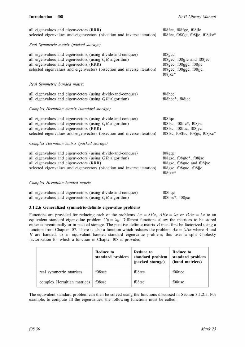
all eigenvalues and eigenvectors (RRR) f08fec, f08fgc, f08jlcselected eigenvalues and eigenvectors (bisection and inverse iteration) f08fec, f08fgc, f08jjc, f08jkc*

Real Symmetric matrix (packed storage)

all eigenvalues and eigenvectors (using divide-and-conquer) f08gccall eigenvalues and eigenvectors (using QR algorithm) f08gec, f08gfc and f08jecall eigenvalues and eigenvectors (RRR) f08gec, f08ggc, f08jlcselected eigenvalues and eigenvectors (bisection and inverse iteration) f08gec, f08ggc, f08jjc,

f08jkc*

Real Symmetric banded matrix

all eigenvalues and eigenvectors (using divide-and-conquer) f08hccall eigenvalues and eigenvectors (using QR algorithm) f08hec*, f08jec

Complex Hermitian matrix (standard storage)

all eigenvalues and eigenvectors (using divide-and-conquer) f08fqcall eigenvalues and eigenvectors (using QR algorithm) f08fsc, f08ftc*, f08jscall eigenvalues and eigenvectors (RRR) f08fsc, f08fuc, f08jycselected eigenvalues and eigenvectors (bisection and inverse iteration) f08fsc, f08fuc, f08jjc, f08jxc*

Complex Hermitian matrix (packed storage)

all eigenvalues and eigenvectors (using divide-and-conquer) f08gqcall eigenvalues and eigenvectors (using QR algorithm) f08gsc, f08gtc*, f08jscall eigenvalues and eigenvectors (RRR) f08gsc, f08guc and f08jycselected eigenvalues and eigenvectors (bisection and inverse iteration) f08gsc, f08guc, f08jjc,

f08jxc*

Complex Hermitian banded matrix

all eigenvalues and eigenvectors (using divide-and-conquer) f08hqcall eigenvalues and eigenvectors (using QR algorithm) f08hsc*, f08jsc

3.1.2.6 Generalized symmetric-definite eigenvalue problems

Functions are provided for reducing each of the problems Ax ¼ �Bx, ABx ¼ �x or BAx ¼ �x to anequivalent standard eigenvalue problem Cy ¼ �y. Different functions allow the matrices to be storedeither conventionally or in packed storage. The positive definite matrix B must first be factorized using afunction from Chapter f07. There is also a function which reduces the problem Ax ¼ �Bx where A andB are banded, to an equivalent banded standard eigenvalue problem; this uses a split Choleskyfactorization for which a function in Chapter f08 is provided.

Reduce tostandard problem

Reduce tostandard problem(packed storage)

Reduce tostandard problem(band matrices)

real symmetric matrices f08sec f08tec f08uec

complex Hermitian matrices f08ssc f08tsc f08usc

The equivalent standard problem can then be solved using the functions discussed in Section 3.1.2.5. Forexample, to compute all the eigenvalues, the following functions must be called:


f08.30 Mark 25

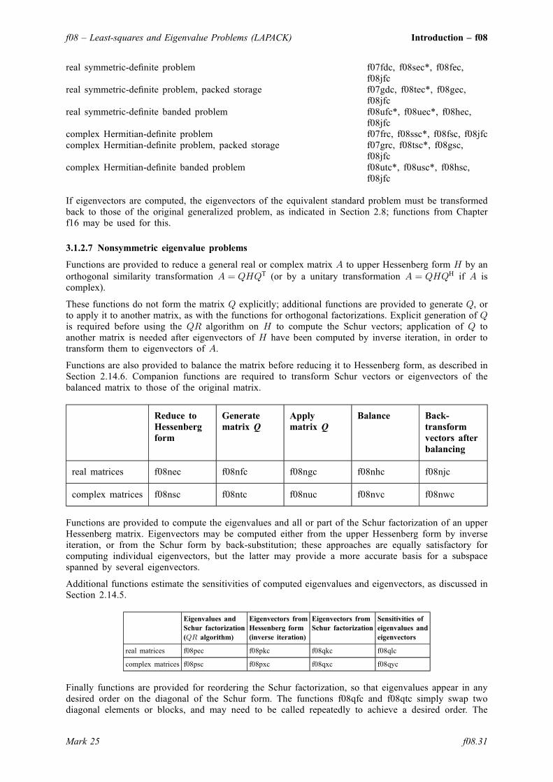
real symmetric-definite problem f07fdc, f08sec*, f08fec,f08jfc

real symmetric-definite problem, packed storage f07gdc, f08tec*, f08gec,f08jfc

real symmetric-definite banded problem f08ufc*, f08uec*, f08hec,f08jfc

complex Hermitian-definite problem f07frc, f08ssc*, f08fsc, f08jfccomplex Hermitian-definite problem, packed storage f07grc, f08tsc*, f08gsc,

f08jfccomplex Hermitian-definite banded problem f08utc*, f08usc*, f08hsc,

f08jfc

If eigenvectors are computed, the eigenvectors of the equivalent standard problem must be transformedback to those of the original generalized problem, as indicated in Section 2.8; functions from Chapterf16 may be used for this.

3.1.2.7 Nonsymmetric eigenvalue problems

Functions are provided to reduce a general real or complex matrix A to upper Hessenberg form H by anorthogonal similarity transformation A ¼ QHQT (or by a unitary transformation A ¼ QHQH if A iscomplex).

These functions do not form the matrix Q explicitly; additional functions are provided to generate Q, orto apply it to another matrix, as with the functions for orthogonal factorizations. Explicit generation of Qis required before using the QR algorithm on H to compute the Schur vectors; application of Q toanother matrix is needed after eigenvectors of H have been computed by inverse iteration, in order totransform them to eigenvectors of A.

Functions are also provided to balance the matrix before reducing it to Hessenberg form, as described inSection 2.14.6. Companion functions are required to transform Schur vectors or eigenvectors of thebalanced matrix to those of the original matrix.

Reduce toHessenbergform

Generatematrix Q

Applymatrix Q

Balance Back-transformvectors afterbalancing

real matrices f08nec f08nfc f08ngc f08nhc f08njc

complex matrices f08nsc f08ntc f08nuc f08nvc f08nwc

Functions are provided to compute the eigenvalues and all or part of the Schur factorization of an upperHessenberg matrix. Eigenvectors may be computed either from the upper Hessenberg form by inverseiteration, or from the Schur form by back-substitution; these approaches are equally satisfactory forcomputing individual eigenvectors, but the latter may provide a more accurate basis for a subspacespanned by several eigenvectors.

Additional functions estimate the sensitivities of computed eigenvalues and eigenvectors, as discussed inSection 2.14.5.

Eigenvalues andSchur factorization(QR algorithm)

Eigenvectors fromHessenberg form(inverse iteration)

Eigenvectors fromSchur factorization

Sensitivities ofeigenvalues andeigenvectors

real matrices f08pec f08pkc f08qkc f08qlc

complex matrices f08psc f08pxc f08qxc f08qyc

Finally functions are provided for reordering the Schur factorization, so that eigenvalues appear in anydesired order on the diagonal of the Schur form. The functions f08qfc and f08qtc simply swap twodiagonal elements or blocks, and may need to be called repeatedly to achieve a desired order. The


Mark 25 f08.31

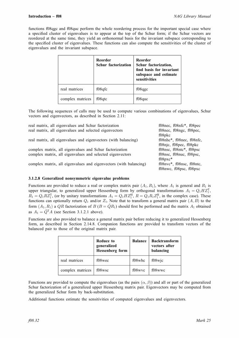
functions f08qgc and f08quc perform the whole reordering process for the important special case wherea specified cluster of eigenvalues is to appear at the top of the Schur form; if the Schur vectors arereordered at the same time, they yield an orthonormal basis for the invariant subspace corresponding tothe specified cluster of eigenvalues. These functions can also compute the sensitivities of the cluster ofeigenvalues and the invariant subspace.

ReorderSchur factorization

ReorderSchur factorization,find basis for invariantsubspace and estimatesensitivities

real matrices f08qfc f08qgc

complex matrices f08qtc f08quc

The following sequences of calls may be used to compute various combinations of eigenvalues, Schurvectors and eigenvectors, as described in Section 2.11:

real matrix, all eigenvalues and Schur factorization f08nec, f08nfc*, f08pecreal matrix, all eigenvalues and selected eigenvectors f08nec, f08ngc, f08pec,

f08pkcreal matrix, all eigenvalues and eigenvectors (with balancing) f08nhc*, f08nec, f08nfc,

f08njc, f08pec, f08pkccomplex matrix, all eigenvalues and Schur factorization f08nsc, f08ntc*, f08psccomplex matrix, all eigenvalues and selected eigenvectors f08nsc, f08nuc, f08psc,

f08pxc*complex matrix, all eigenvalues and eigenvectors (with balancing) f08nvc*, f08nsc, f08ntc,

f08nwc, f08psc, f08pxc

3.1.2.8 Generalized nonsymmetric eigenvalue problems

Functions are provided to reduce a real or complex matrix pair A1; R1ð Þ, where A1 is general and R1 isupper triangular, to generalized upper Hessenberg form by orthogonal transformations A1 ¼ Q1HZ

T1 ,

R1 ¼ Q1RZT1 , (or by unitary transformations A1 ¼ Q1HZ

H1 , R ¼ Q1R1Z

H1 , in the complex case). These

functions can optionally return Q1 and/or Z1. Note that to transform a general matrix pair A;Bð Þ to the

form A1; R1ð Þ a QR factorization of B (B ¼ ~QR1) should first be performed and the matrix A1 obtained

as A1 ¼ ~QTA (see Section 3.1.2.1 above).

Functions are also provided to balance a general matrix pair before reducing it to generalized Hessenbergform, as described in Section 2.14.8. Companion functions are provided to transform vectors of thebalanced pair to those of the original matrix pair.

Reduce togeneralizedHessenberg form

Balance Backtransformvectors afterbalancing

real matrices f08wec f08whc f08wjc

complex matrices f08wsc f08wvc f08wwc

Functions are provided to compute the eigenvalues (as the pairs �; �ð Þ) and all or part of the generalizedSchur factorization of a generalized upper Hessenberg matrix pair. Eigenvectors may be computed fromthe generalized Schur form by back-substitution.

Additional functions estimate the sensitivities of computed eigenvalues and eigenvectors.


f08.32 Mark 25

Eigenvalues andgeneralized Schurfactorization(QZ algorithm)

Eigenvectors fromgeneralized Schurfactorization

Sensitivities ofeigenvalues andeigenvectors

real matrices f08xec f08ykc f08ylc

complex matrices f08xsc f08yxc f08yyc

Finally, functions are provided for reordering the generalized Schur factorization so that eigenvaluesappear in any desired order on the diagonal of the generalized Schur form. f08yfc and f08ytc simplyswap two diagonal elements or blocks, and may need to be called repeatedly to achieve a desired order.f08ygc and f08yuc perform the whole reordering process for the important special case where a specifiedcluster of eigenvalues is to appear at the top of the generalized Schur form; if the Schur vectors arereordered at the same time, they yield an orthonormal basis for the deflating subspace corresponding tothe specified cluster of eigenvalues. These functions can also compute the sensitivities of the cluster ofeigenvalues and the deflating subspace.

Reorder generalized Schurfactorization

Reorder generalized Schurfactorization, find basis fordeflating subspace andestimate sensitivites

real matrices f08yfc f08ygc

complex matrices f08ytc f08yuc

The following sequences of calls may be used to compute various combinations of eigenvalues,generalized Schur vectors and eigenvectors

real matrix pair, all eigenvalues (with balancing) f08aec, f08agc (or f08abc,f08acc), f08wec, f08whc,f08xec*

real matrix pair, all eigenvalues and generalized Schur factorization f08aec, f08afc, f08agc (orf08abc, f08acc), f08wec,f08xec

real matrix pair, all eigenvalues and eigenvectors (with balancing) f16qfc, f16qhc, f08aec,f08afc, f08agc (or f08abc,f08acc), f08wec, f08whc,f08xec, f08ykc*, f08wjc

complex matrix pair, all eigenvalues (with balancing) f08asc, f08auc (or f08apc,f08aqc), f08wsc, f08wvc,f08xsc*

complex matrix pair, all eigenvalues and generalized Schur factorization f08asc, f08atc, f08auc (orf08apc, f08aqc), f08wsc,f08xsc

complex matrix pair, all eigenvalues and eigenvectors (with balancing) f16tfc, f16thc, f08asc, f08atc,f08auc (or f08apc, f08aqc),f08wsc, f08wvc, f08xsc,f08yxc*, f08wwc

3.1.2.9 The Sylvester equation and the generalized Sylvester equation

Functions are provided to solve the real or complex Sylvester equation AX �XB ¼ C, where A and Bare upper quasi-triangular if real, or upper triangular if complex. To solve the general form of theSylvester equation in which A and B are general square matrices, A and B must be reduced to upper(quasi-) triangular form by the Schur factorization, using functions described in Section 3.1.2.7. Formore details, see the documents for the functions listed below.


Mark 25 f08.33

Solve the Sylvester equation

real matrices f08qhc

complex matrices f08qvc

Functions are also provided to solve the real or complex generalized Sylvester equations

AR� LB ¼ C; DR� LE ¼ F;

where the pairs A;Dð Þ and B;Eð Þ are in generalized Schur form. To solve the general form of thegeneralized Sylvester equation in which A;Dð Þ and B;Eð Þ are general matrix pairs, A;Dð Þ and B;Eð Þmust first be reduced to generalized Schur form.

Solve the generalized Sylvester equation

real matrices f08yhc

complex matrices f08yvc

3.2 NAG Names and LAPACK Names

The functions may be called either by their NAG short names or by their NAG long names whichcontain their double precision LAPACK names.

References to Chapter f08 functions in the manual normally include the LAPACK double precisionnames, for example nag_dgeqrf (f08aec). The LAPACK routine names follow a simple scheme. Eachname has the structure xyyzzz, where the components have the following meanings:

– the initial letter x indicates the data type (real or complex) and precision:

s – real, single precision

d – real, double precision

c – complex, single precision

z – complex, double precision

– the second and third letters yy indicate the type of the matrix A or matrix pair A;Bð Þ (and in somecases the storage scheme):

bd – bidiagonal

di – diagonal

gb – general band

ge – general

gg – general pair (B may be triangular)

hb – (complex) Hermitian band

he – Hermitian

hg – generalized upper Hessenberg

hp – Hermitian (packed storage)

hs – upper Hessenberg

op – (real) orthogonal (packed storage)

or – (real) orthogonal

pt – symmetric or Hermitian positive definite tridiagonal


f08.34 Mark 25

sb – (real) symmetric band

sp – symmetric (packed storage)

st – (real) symmetric tridiagonal

sy – symmetric

tg – triangular pair (one may be quasi-triangular)

tp – triangular-pentagonal

tr – triangular (or quasi-triangular)

un – (complex) unitary

up – (complex) unitary (packed storage)

– the last three letters zzz indicate the computation performed. For example, qrf is a QR factorization.

Thus the function nag_dgeqrf performs a QR factorization of a real general matrix; the correspondingfunction for a complex general matrix is nag_zgeqrf.

3.3 Matrix Storage Schemes

In this chapter the following storage schemes are used for matrices:

– conventional storage in a two-dimensional array;

– packed storage for symmetric or Hermitian matrices;

– packed storage for orthogonal or unitary matrices;

– band storage for general, symmetric or Hermitian band matrices;

– storage of bidiagonal, symmetric or Hermitian tridiagonal matrices in two one-dimensionalarrays.

These storage schemes are compatible with those used in Chapters f07 and f16, but different schemes forpacked, band and tridiagonal storage are used in a few older functions in Chapters f01, f02, f03 and f04.

3.3.1 Conventional storage

Please see Section 3.3.1 in the f07 Chapter Introduction for full details.

3.3.2 Packed storage


3.3.3 Band storage


3.3.4 Tridiagonal and bidiagonal matrices

A symmetric tridiagonal or bidiagonal matrix is stored in two one-dimensional arrays, one of length ncontaining the diagonal elements, and one of length n� 1 containing the off-diagonal elements. (Olderfunctions in Chapter f02 store the off-diagonal elements in elements 2 : n of a vector of length n.)

3.3.5 Real diagonal elements of complex matrices


3.3.6 Representation of orthogonal or unitary matrices

A real orthogonal or complex unitary matrix (usually denoted Q) is often represented in the NAG CLibrary as a product of elementary reflectors – also referred to as elementary Householder matrices(usually denoted Hi). For example,


Mark 25 f08.35

Q ¼ H1H2 � � �Hk:

You need not be aware of the details, because functions are provided to work with this representation,either to generate all or part of Q explicitly, or to multiply a given matrix by Q or QT (QH in thecomplex case) without forming Q explicitly.

Nevertheless, the following further details may occasionally be useful.

An elementary reflector (or elementary Householder matrix) H of order n is a unitary matrix of the form

H ¼ I � �vvH ð4Þ

where � is a scalar, and v is an n-element vector, with �j j2 vk k22 ¼ 2� Re �ð Þ; v is often referred to as the

Householder vector. Often v has several leading or trailing zero elements, but for the purpose of thisdiscussion assume that H has no such special structure.

There is some redundancy in the representation 4ð Þ, which can be removed in various ways. Therepresentation used in Chapter f08 and in LAPACK (which differs from those used in some of thefunctions in Chapters f01, f02 and f04) sets v1 ¼ 1; hence v1 need not be stored. In real arithmetic,1 � � � 2, except that � ¼ 0 implies H ¼ I.

In complex arithmetic, � may be complex, and satisfies 1 � Re �ð Þ � 2 and � � 1j j � 1. Thus a complexH is not Hermitian (as it is in other representations), but it is unitary, which is the important property.The advantage of allowing � to be complex is that, given an arbitrary complex vector x;H can becomputed so that

HHx ¼ � 1; 0; . . . ; 0ð ÞT

with real �. This is useful, for example, when reducing a complex Hermitian matrix to real symmetrictridiagonal form, or a complex rectangular matrix to real bidiagonal form.

3.4 Argument Conventions

3.4.1 Option arguments

In addition to the order argument of type Nag_OrderType, most functions in this Chapter have one ormore option arguments of various types; only options of the correct type may be supplied.

For example,

nag_dsytrd(Nag_RowMajor,Nag_Upper,...)

3.4.2 Problem dimensions

It is permissible for the problem dimensions (for example, m or n) to be passed as zero, in which casethe computation (or part of it) is skipped. Negative dimensions are regarded as an error.


f08.36 Mark 25

4 Decision Trees

The following decision trees are principally for the computation (general purpose) functions.

4.1 General Purpose Functions (eigenvalues and eigenvectors)

Tree 1: Real Symmetric Eigenvalue Problems

Are eigenvalues onlyrequired? yes

Are all the eigenvaluesrequired? yes

Is A tridiagonal?yes

f08jcc or f08jfc

no

Is A band matrix?yes

(f08hec and f08jfc) orf08hcc

no

Is one triangle of A stored asa linear array? yes

(f08gec and f08jfc) orf08gcc

no

(f08fec and f08jfc) or f08facor f08fcc

no


f08jjc

no

Is A a band matrix?yes

f08hec and f08jjc

no


f08gec and f08jjc

no

(f08fec and f08jjc) or f08fbc

no

Are all eigenvalues andeigenvectors required? yes


f08jec, f08jcc, f08jhc orf08jlc

no


(f08hec and f08jec) orf08hcc

no


(f08gec, f08gfc and f08jec)or f08gcc

no

(f08fec, f08ffc and f08jec) orf08fac or f08fcc

no


f08jjc and f08jkc

no


f08gec, f08jjc, f08jkc andf08ggc

no

(f08fec, f08jjc, f08jkc andf08fgc) or f08fbc


Mark 25 f08.37

Tree 2: Real Generalized Symmetric-definite Eigenvalue Problems



Are A and B band matrices?yes

f08ufc, f08uec, f08hec andf08jfc

no

Are A and B stored with onetriangle as a linear array? yes

f07gdc, f08tec, f08gec andf08jfc

no

f07fdc, f08sec, f08fec andf08jfc

no


f08ufc, f08uec, f08hec andf08jjc

no


f07gdc, f08tec, f08gec andf08jjc

no

f07fdc, f08sec, f08gec andf08jjc

no



f07gdc, f08tec, f08gec,f08gfc, f08jec and f16plc

no

f07fdc, f08sec, f08fec,f08ffc, f08jec and f16yjc

no


f08ufc, f08uec, f08hec,f08jkc and f16yjc

no


f07gdc, f08tec, f08gec,f08jjc, f08jkc, f08ggc and

f16plc

no

f07fdc, f08sec, f08fec,f08jjc, f08jkc, f08fgc and

f16yjc

Note: the functions for band matrices only handle the problem Ax ¼ �Bx; the other functions handle allthree types of problems (Ax ¼ �Bx, ABx ¼ �x or BAx ¼ �x) except that, if the problem is BAx ¼ �xand eigenvectors are required, f16phc must be used instead of f16plc and f16yfc instead of f16yjc.


f08.38 Mark 25

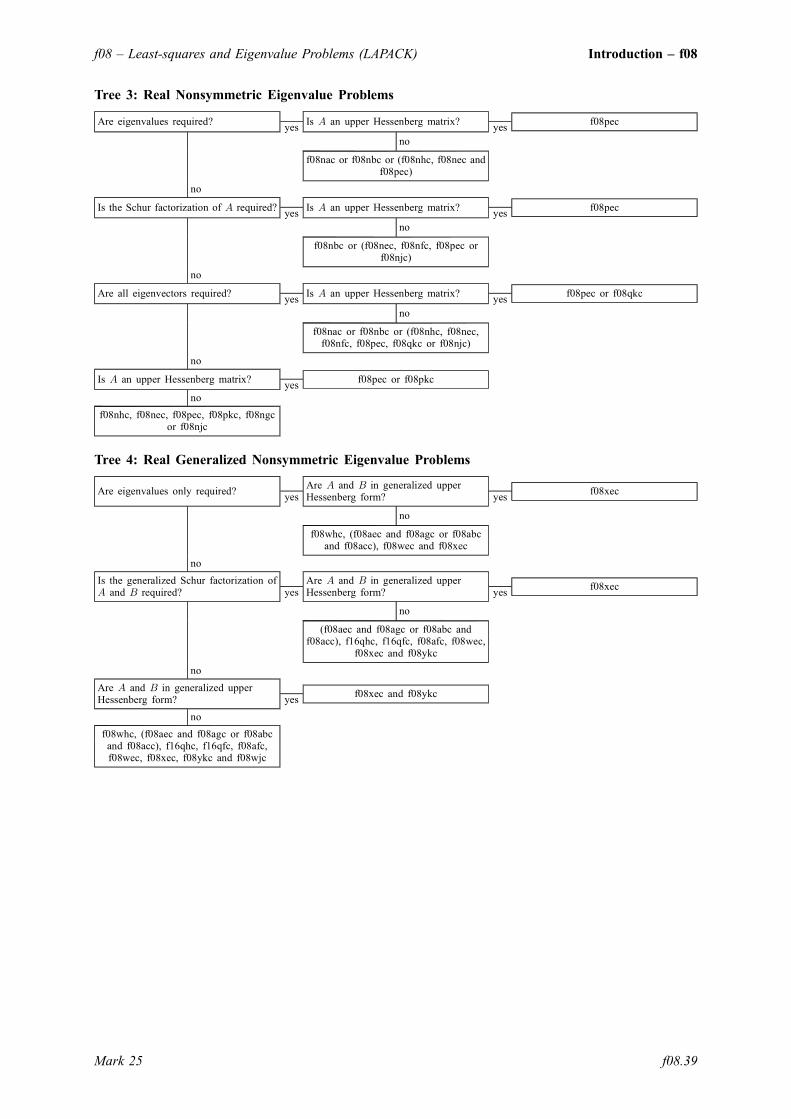
Tree 3: Real Nonsymmetric Eigenvalue Problems

Are eigenvalues required?yes

Is A an upper Hessenberg matrix?yes

f08pec

no

f08nac or f08nbc or (f08nhc, f08nec andf08pec)

no

Is the Schur factorization of A required?yes


f08pec

no

f08nbc or (f08nec, f08nfc, f08pec orf08njc)

no

Are all eigenvectors required?yes


f08pec or f08qkc

no

f08nac or f08nbc or (f08nhc, f08nec,f08nfc, f08pec, f08qkc or f08njc)

no


f08pec or f08pkc

no

f08nhc, f08nec, f08pec, f08pkc, f08ngcor f08njc

Tree 4: Real Generalized Nonsymmetric Eigenvalue Problems

Are eigenvalues only required?yes

Are A and B in generalized upperHessenberg form? yes

f08xec

no

f08whc, (f08aec and f08agc or f08abcand f08acc), f08wec and f08xec

no

Is the generalized Schur factorization ofA and B required? yes


f08xec

no

(f08aec and f08agc or f08abc andf08acc), f16qhc, f16qfc, f08afc, f08wec,

f08xec and f08ykc

no


f08xec and f08ykc

no

f08whc, (f08aec and f08agc or f08abcand f08acc), f16qhc, f16qfc, f08afc,f08wec, f08xec, f08ykc and f08wjc


Mark 25 f08.39

Tree 5: Complex Hermitian Eigenvalue Problems




(f08hsc and f08jfc) orf08hqc

no


(f08gsc and f08jfc) orf08gqc

no

(f08fsc and f08jfc) or f08fqc

no


f08hsc and f08jjc

no


f08gsc and f08jjc

no

f08fsc and f08jjc

no



(f08hsc and f08jsc) orf08hqc

no


(f08gsc, f08gtc and f08jsc)or f08gqc

no

(f08fsc, f08ftc and f08jsc) orf08fqc

no


f08gsc, f08jjc, f08jxc andf08guc

no

f08fsc, f08jjc, f08jxc andf08fuc

Tree 6: Complex Generalized Hermitian-definite Eigenvalue Problems


Are all eigenvalues required?yes


f07grc, f08tsc, f08gsc andf08jfc

no

f07frc, f08ssc, f08fsc andf08jfc

no


f07grc, f08tsc, f08gsc andf08jjc

no

f07frc, f08ssc, f08gsc andf08jjc

no



f07grc, f08tsc, f08gsc,f08gtc and f16psc

no

f07frc, f08ssc, f08fsc, f08ftc,f08jsc and f16zjc

no


f07grc, f08tsc, f08gsc,f08jjc, f08jxc, f08guc and

f16slc

no

f07frc, f08ssc, f08fsc, f08jjc,f08jxc, f08fuc and f16zjc


f08.40 Mark 25

Tree 7: Complex non-Hermitian Eigenvalue Problems



f08psc

no

f08nvc, f08nsc and f08psc

no

Is the Schur factorization of A required?yes


f08psc

no

f08nsc, f08ntc, f08psc and f08nwc

no

Are all eigenvectors required?yes


f08psc and f08qxc

no

f08nvc, f08nsc, f08ntc, f08psc, f08qxcand f08nwc

no


f08psc and f08pxc

no

f08nvc, f08nsc, f08psc, f08pxc, f08nucand f08nwc

Tree 8: Complex Generalized non-Hermitian Eigenvalue Problems



f08xsc

no

f08wvc, (f08asc and f08auc or f08apcand f08aqc), f08wsc and f08xsc

no

Is the generalized Schur factorization ofA and B required? yes


f08xsc

no

(f08asc and f08auc or f08apc andf08aqc), f16thc, f16tfc, f08atc, f08wsc,

f08xsc and f08yxc

no


f08xsc and f08yxc

no

f08wvc, (f08asc and f08auc or f08apcand f08aqc), f16thc, f16tfc, f08atc,

f08wsc, f08xsc, f08yxc and f08wwc


Mark 25 f08.41

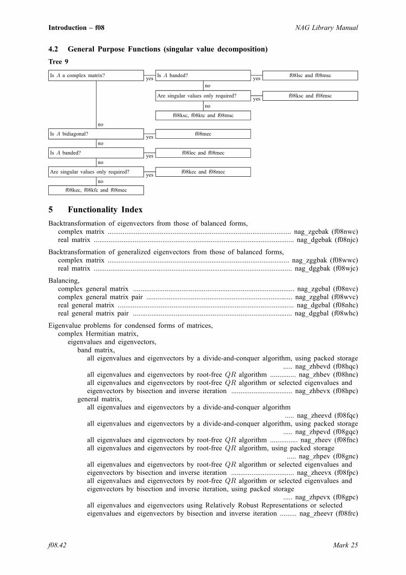
4.2 General Purpose Functions (singular value decomposition)

Tree 9

Is A a complex matrix?yes

Is A banded?yes

f08lsc and f08msc

no

Are singular values only required?yes

f08ksc and f08msc

no

f08ksc, f08ktc and f08msc

no

Is A bidiagonal?yes

f08mec

no

Is A banded?yes

f08lec and f08mec

no

Are singular values only required?yes

f08kec and f08mec

no

f08kec, f08kfc and f08mec

5 Functionality Index

Backtransformation of eigenvectors from those of balanced forms,complex matrix ................................................................................................... nag_zgebak (f08nwc)real matrix ............................................................................................................ nag_dgebak (f08njc)

Backtransformation of generalized eigenvectors from those of balanced forms,complex matrix .................................................................................................. nag_zggbak (f08wwc)real matrix ........................................................................................................... nag_dggbak (f08wjc)

Balancing,complex general matrix ....................................................................................... nag_zgebal (f08nvc)complex general matrix pair ............................................................................... nag_zggbal (f08wvc)real general matrix ............................................................................................... nag_dgebal (f08nhc)real general matrix pair ...................................................................................... nag_dggbal (f08whc)

Eigenvalue problems for condensed forms of matrices,complex Hermitian matrix,

eigenvalues and eigenvectors,band matrix,

all eigenvalues and eigenvectors by a divide-and-conquer algorithm, using packed storage..... nag_zhbevd (f08hqc)

all eigenvalues and eigenvectors by root-free QR algorithm .............. nag_zhbev (f08hnc)all eigenvalues and eigenvectors by root-free QR algorithm or selected eigenvalues andeigenvectors by bisection and inverse iteration ................................. nag_zhbevx (f08hpc)

general matrix,all eigenvalues and eigenvectors by a divide-and-conquer algorithm

..... nag_zheevd (f08fqc)all eigenvalues and eigenvectors by a divide-and-conquer algorithm, using packed storage

..... nag_zhpevd (f08gqc)all eigenvalues and eigenvectors by root-free QR algorithm ............... nag_zheev (f08fnc)all eigenvalues and eigenvectors by root-free QR algorithm, using packed storage

..... nag_zhpev (f08gnc)all eigenvalues and eigenvectors by root-free QR algorithm or selected eigenvalues andeigenvectors by bisection and inverse iteration .................................. nag_zheevx (f08fpc)all eigenvalues and eigenvectors by root-free QR algorithm or selected eigenvalues andeigenvectors by bisection and inverse iteration, using packed storage

..... nag_zhpevx (f08gpc)all eigenvalues and eigenvectors using Relatively Robust Representations or selectedeigenvalues and eigenvectors by bisection and inverse iteration ......... nag_zheevr (f08frc)


f08.42 Mark 25

eigenvalues only,band matrix,

all eigenvalues by the Pal–Walker–Kahan variant of the QL or QR algorithm..... nag_zhbev (f08hnc)

all eigenvalues by the Pal–Walker–Kahan variant of the QL or QR algorithm, or selectedeigenvalues by bisection ..................................................................... nag_zhbevx (f08hpc)all eigenvalues by the Pal–Walker–Kahan variant of the QL or QR algorithm, usingpacked storage ..................................................................................... nag_zhbevd (f08hqc)

general matrix,all eigenvalues by the Pal–Walker–Kahan variant of the QL or QR algorithm

..... nag_zheev (f08fnc)all eigenvalues by the Pal–Walker–Kahan variant of the QL or QR algorithm, or selectedeigenvalues by bisection ...................................................................... nag_zheevx (f08fpc)all eigenvalues by the Pal–Walker–Kahan variant of the QL or QR algorithm, or selectedeigenvalues by bisection, using packed storage ................................. nag_zhpevx (f08gpc)all eigenvalues by the Pal–Walker–Kahan variant of the QL or QR algorithm, usingpacked storage ....................................................................................... nag_zhpev (f08gnc)

complex upper Hessenberg matrix, reduced from complex general matrix,eigenvalues and Schur factorization ............................................................... nag_zhseqr (f08psc)selected right and/or left eigenvectors by inverse iteration ........................... nag_zhsein (f08pxc)

real bidiagonal matrix,singular value decomposition,

after reduction from complex general matrix .......................................... nag_zbdsqr (f08msc)after reduction from real general matrix ................................................. nag_dbdsqr (f08mec)after reduction from real general matrix, using divide-and-conquer ...... nag_dbdsdc (f08mdc)

real symmetric matrix,eigenvalues and eigenvectors,

band matrix,all eigenvalues and eigenvectors by a divide-and-conquer algorithm

..... nag_dsbevd (f08hcc)all eigenvalues and eigenvectors by root-free QR algorithm .............. nag_dsbev (f08hac)all eigenvalues and eigenvectors by root-free QR algorithm or selected eigenvalues andeigenvectors by bisection and inverse iteration .................................. nag_dsbevx (f08hbc)

general matrix,all eigenvalues and eigenvectors by a divide-and-conquer algorithm

..... nag_dsyevd (f08fcc)all eigenvalues and eigenvectors by a divide-and-conquer algorithm, using packed storage

..... nag_dspevd (f08gcc)all eigenvalues and eigenvectors by root-free QR algorithm ............... nag_dsyev (f08fac)all eigenvalues and eigenvectors by root-free QR algorithm, using packed storage

..... nag_dspev (f08gac)all eigenvalues and eigenvectors by root-free QR algorithm or selected eigenvalues andeigenvectors by bisection and inverse iteration .................................. nag_dsyevx (f08fbc)all eigenvalues and eigenvectors by root-free QR algorithm or selected eigenvalues andeigenvectors by bisection and inverse iteration, using packed storage

..... nag_dspevx (f08gbc)all eigenvalues and eigenvectors using Relatively Robust Representations or selectedeigenvalues and eigenvectors by bisection and inverse iteration ........ nag_dsyevr (f08fdc)

eigenvalues only,band matrix,

all eigenvalues by the Pal–Walker–Kahan variant of the QL or QR algorithm..... nag_dsbev (f08hac)

all eigenvalues by the Pal–Walker–Kahan variant of the QL or QR algorithm, or selectedeigenvalues by bisection ..................................................................... nag_dsbevx (f08hbc)

general matrix,all eigenvalues by the Pal–Walker–Kahan variant of the QL or QR algorithm

..... nag_dsyev (f08fac)all eigenvalues by the Pal–Walker–Kahan variant of the QL or QR algorithm, or selectedeigenvalues by bisection ...................................................................... nag_dsyevx (f08fbc)


Mark 25 f08.43

all eigenvalues by the Pal–Walker–Kahan variant of the QL or QR algorithm, or selectedeigenvalues by bisection, using packed storage ................................. nag_dspevx (f08gbc)all eigenvalues by the Pal–Walker–Kahan variant of the QL or QR algorithm, usingpacked storage ....................................................................................... nag_dspev (f08gac)

real symmetric tridiagonal matrix,eigenvalues and eigenvectors,

after reduction from complex Hermitian matrix,all eigenvalues and eigenvectors ............................................................ nag_zsteqr (f08jsc)all eigenvalues and eigenvectors, positive definite matrix ................... nag_zpteqr (f08juc)all eigenvalues and eigenvectors, using divide-and-conquer ................ nag_zstedc (f08jvc)all eigenvalues and eigenvectors, using Relatively Robust Representations

..... nag_zstegr (f08jyc)selected eigenvectors by inverse iteration ............................................. nag_zstein (f08jxc)

all eigenvalues and eigenvectors ................................................................. nag_dsteqr (f08jec)all eigenvalues and eigenvectors, by divide-and-conquer .......................... nag_dstedc (f08jhc)all eigenvalues and eigenvectors, positive definite matrix ........................ nag_dpteqr (f08jgc)all eigenvalues and eigenvectors, using Relatively Robust Representations

..... nag_dstegr (f08jlc)all eigenvalues and eigenvectors by a divide-and-conquer algorithm ...... nag_dstevd (f08jcc)all eigenvalues and eigenvectors by root-free QR algorithm ..................... nag_dstev (f08jac)all eigenvalues and eigenvectors by root-free QR algorithm or selected eigenvalues andeigenvectors by bisection and inverse iteration ......................................... nag_dstevx (f08jbc)all eigenvalues and eigenvectors using Relatively Robust Representations or selectedeigenvalues and eigenvectors by bisection and inverse iteration .............. nag_dstevr (f08jdc)selected eigenvectors by inverse iteration .................................................. nag_dstein (f08jkc)

eigenvalues only,all eigenvalues by root-free QR algorithm ................................................. nag_dsterf (f08jfc)all eigenvalues by the Pal–Walker–Kahan variant of the QL or QR algorithm

..... nag_dstev (f08jac)all eigenvalues by the Pal–Walker–Kahan variant of the QL or QR algorithm, or selectedeigenvalues by bisection ............................................................................ nag_dstevx (f08jbc)selected eigenvalues by bisection ............................................................... nag_dstebz (f08jjc)

real upper Hessenberg matrix, reduced from real general matrix,eigenvalues and Schur factorization ............................................................... nag_dhseqr (f08pec)selected right and/or left eigenvectors by inverse iteration ........................... nag_dhsein (f08pkc)

Eigenvalue problems for nonsymmetric matrices,complex matrix,

all eigenvalues, Schur form, Schur vectors and reciprocal condition numbers..... nag_zgeesx (f08ppc)

all eigenvalues, Schur form and Schur vectors ............................................... nag_zgees (f08pnc)all eigenvalues and left/right eigenvectors ...................................................... nag_zgeev (f08nnc)all eigenvalues and left/right eigenvectors, plus balancing transformation and reciprocal conditionnumbers .......................................................................................................... nag_zgeevx (f08npc)

real matrix,all eigenvalues, real Schur form, Schur vectors and reciprocal condition numbers

..... nag_dgeesx (f08pbc)all eigenvalues, real Schur form and Schur vectors ....................................... nag_dgees (f08pac)all eigenvalues and left/right eigenvectors ...................................................... nag_dgeev (f08nac)all eigenvalues and left/right eigenvectors, plus balancing transformation and reciprocal conditionnumbers .......................................................................................................... nag_dgeevx (f08nbc)

Eigenvalues and generalized Schur factorization,complex generalized upper Hessenberg form ..................................................... nag_zhgeqz (f08xsc)real generalized upper Hessenberg form ............................................................ nag_dhgeqz (f08xec)

General Gauss–Markov linear model,solves a complex general Gauss–Markov linear model problem ..................... nag_zggglm (f08zpc)solves a real general Gauss–Markov linear model problem ............................. nag_dggglm (f08zbc)


f08.44 Mark 25

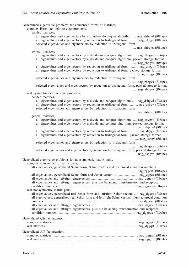
Generalized eigenvalue problems for condensed forms of matrices,complex Hermitian-definite eigenproblems,

banded matrices,all eigenvalues and eigenvectors by a divide-and-conquer algorithm ..... nag_zhbgvd (f08uqc)all eigenvalues and eigenvectors by reduction to tridiagonal form .......... nag_zhbgv (f08unc)selected eigenvalues and eigenvectors by reduction to tridiagonal form

..... nag_zhbgvx (f08upc)general matrices,

all eigenvalues and eigenvectors by a divide-and-conquer algorithm ..... nag_zhegvd (f08sqc)all eigenvalues and eigenvectors by a divide-and-conquer algorithm, packed storage format

..... nag_zhpgvd (f08tqc)all eigenvalues and eigenvectors by reduction to tridiagonal form .......... nag_zhegv (f08snc)all eigenvalues and eigenvectors by reduction to tridiagonal form, packed storage format

..... nag_zhpgv (f08tnc)selected eigenvalues and eigenvectors by reduction to tridiagonal form

..... nag_zhegvx (f08spc)selected eigenvalues and eigenvectors by reduction to tridiagonal form, packed storage format

..... nag_zhpgvx (f08tpc)real symmetric-definite eigenproblems,

banded matrices,all eigenvalues and eigenvectors by a divide-and-conquer algorithm ..... nag_dsbgvd (f08ucc)all eigenvalues and eigenvectors by reduction to tridiagonal form .......... nag_dsbgv (f08uac)selected eigenvalues and eigenvectors by reduction to tridiagonal form

..... nag_dsbgvx (f08ubc)general matrices,

all eigenvalues and eigenvectors by a divide-and-conquer algorithm ..... nag_dsygvd (f08scc)all eigenvalues and eigenvectors by a divide-and-conquer algorithm, packed storage format

..... nag_dspgvd (f08tcc)all eigenvalues and eigenvectors by reduction to tridiagonal form .......... nag_dsygv (f08sac)all eigenvalues and eigenvectors by reduction to tridiagonal form, packed storage format

..... nag_dspgv (f08tac)selected eigenvalues and eigenvectors by reduction to tridiagonal form

..... nag_dsygvx (f08sbc)selected eigenvalues and eigenvectors by reduction to tridiagonal form, packed storage format

..... nag_dspgvx (f08tbc)

Generalized eigenvalue problems for nonsymmetric matrix pairs,complex nonsymmetric matrix pairs,

all eigenvalues, generalized Schur form, Schur vectors and reciprocal condition numbers..... nag_zggesx (f08xpc)

all eigenvalues, generalized Schur form and Schur vectors ........................... nag_zgges (f08xnc)all eigenvalues and left/right eigenvectors ..................................................... nag_zggev (f08wnc)all eigenvalues and left/right eigenvectors, plus the balancing transformation and reciprocalcondition numbers ......................................................................................... nag_zggevx (f08wpc)

real nonsymmetric matrix pairs,all eigenvalues, generalized real Schur form and left/right Schur vectors ..... nag_dgges (f08xac)all eigenvalues, generalized real Schur form and left/right Schur vectors, plus reciprocal conditionnumbers .......................................................................................................... nag_dggesx (f08xbc)all eigenvalues and left/right eigenvectors ..................................................... nag_dggev (f08wac)all eigenvalues and left/right eigenvectors, plus the balancing transformation and reciprocalcondition numbers ........................................................................................ nag_dggevx (f08wbc)

Generalized QR factorization,complex matrices .................................................................................................. nag_zggqrf (f08zsc)real matrices ......................................................................................................... nag_dggqrf (f08zec)

Generalized RQ factorization,complex matrices ................................................................................................... nag_zggrqf (f08ztc)real matrices .......................................................................................................... nag_dggrqf (f08zfc)


Mark 25 f08.45

Generalized singular value decomposition,after reduction from complex general matrix,

complex triangular or trapezoidal matrix pair ................................................. nag_ztgsja (f08ysc)after reduction from real general matrix,

real triangular or trapezoidal matrix pair ........................................................ nag_dtgsja (f08yec)complex matrix pair ............................................................................................ nag_zggsvd (f08vnc)partitioned orthogonal matrix (CS decomposition) .............................................. nag_dorcsd (f08rac)partitioned unitary matrix (CS decomposition) ................................................... nag_zuncsd (f08rnc)real matrix pair .................................................................................................... nag_dggsvd (f08vac)reduction of a pair of general matrices to triangular or trapezoidal form,

complex matrices ............................................................................................ nag_zggsvp (f08vsc)real matrices ................................................................................................... nag_dggsvp (f08vec)

least squares problems,complex matrices,

apply orthogonal matrix ................................................................................ nag_zunmrz (f08bxc)minimum norm solution using a complete orthogonal factorization ............. nag_zgelsy (f08bnc)minimum norm solution using the singular value decomposition ................. nag_zgelss (f08knc)minimum norm solution using the singular value decomposition (divide-and-conquer)

..... nag_zgelsd (f08kqc)reduction of upper trapezoidal matrix to upper triangular form .................... nag_ztzrzf (f08bvc)

real matrices,apply orthogonal matrix ................................................................................ nag_dormrz (f08bkc)minimum norm solution using a complete orthogonal factorization ............. nag_dgelsy (f08bac)minimum norm solution using the singular value decomposition ................. nag_dgelss (f08kac)minimum norm solution using the singular value decomposition (divide-and-conquer)

..... nag_dgelsd (f08kcc)reduction of upper trapezoidal matrix to upper triangular form .................... nag_dtzrzf (f08bhc)

least squares problems with linear equality constraints,complex matrices,

minimum norm solution subject to linear equality constraints using a generalized RQ factorization..... nag_zgglse (f08znc)

real matrices,minimum norm solution subject to linear equality constraints using a generalized RQ factorization

..... nag_dgglse (f08zac)

Left and right eigenvectors of a pair of matrices,complex upper triangular matrices ...................................................................... nag_ztgevc (f08yxc)real quasi-triangular matrices ............................................................................... nag_dtgevc (f08ykc)

LQ factorization and related operations,complex matrices,

apply unitary matrix ...................................................................................... nag_zunmlq (f08axc)factorization ..................................................................................................... nag_zgelqf (f08avc)form all or part of unitary matrix ................................................................. nag_zunglq (f08awc)

real matrices,apply orthogonal matrix ................................................................................. nag_dormlq (f08akc)factorization ..................................................................................................... nag_dgelqf (f08ahc)form all or part of orthogonal matrix ............................................................. nag_dorglq (f08ajc)

Operations on eigenvectors of a real symmetric or complex Hermitian matrix, or singular vectors of ageneral matrix,

estimate condition numbers ................................................................................... nag_ddisna (f08flc)

Operations on generalized Schur factorization of a general matrix pair,complex matrix,

estimate condition numbers of eigenvalues and/or eigenvectors ................... nag_ztgsna (f08yyc)re-order Schur factorization ............................................................................. nag_ztgexc (f08ytc)re-order Schur factorization, compute generalized eigenvalues and condition numbers

..... nag_ztgsen (f08yuc)


f08.46 Mark 25

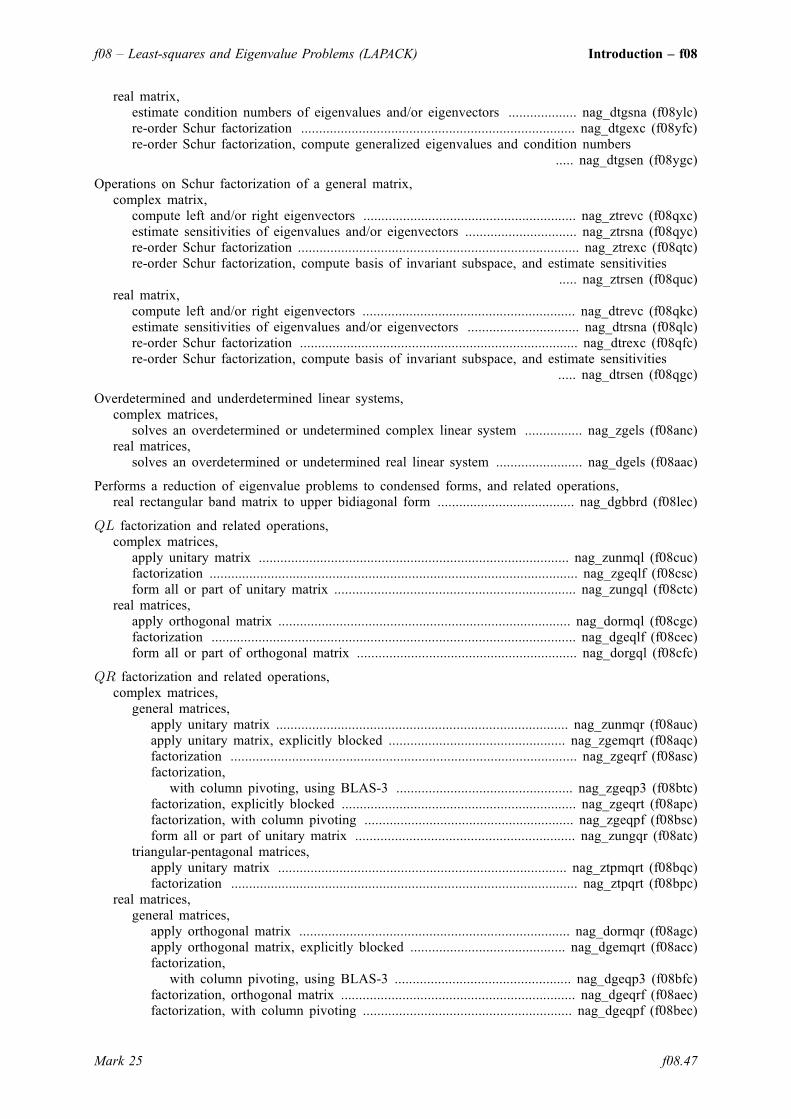
real matrix,estimate condition numbers of eigenvalues and/or eigenvectors ................... nag_dtgsna (f08ylc)re-order Schur factorization ............................................................................ nag_dtgexc (f08yfc)re-order Schur factorization, compute generalized eigenvalues and condition numbers

..... nag_dtgsen (f08ygc)

Operations on Schur factorization of a general matrix,complex matrix,

compute left and/or right eigenvectors ........................................................... nag_ztrevc (f08qxc)estimate sensitivities of eigenvalues and/or eigenvectors ............................... nag_ztrsna (f08qyc)re-order Schur factorization .............................................................................. nag_ztrexc (f08qtc)re-order Schur factorization, compute basis of invariant subspace, and estimate sensitivities

..... nag_ztrsen (f08quc)real matrix,

compute left and/or right eigenvectors ........................................................... nag_dtrevc (f08qkc)estimate sensitivities of eigenvalues and/or eigenvectors ............................... nag_dtrsna (f08qlc)re-order Schur factorization ............................................................................. nag_dtrexc (f08qfc)re-order Schur factorization, compute basis of invariant subspace, and estimate sensitivities

..... nag_dtrsen (f08qgc)

Overdetermined and underdetermined linear systems,complex matrices,

solves an overdetermined or undetermined complex linear system ................ nag_zgels (f08anc)real matrices,

solves an overdetermined or undetermined real linear system ........................ nag_dgels (f08aac)

Performs a reduction of eigenvalue problems to condensed forms, and related operations,real rectangular band matrix to upper bidiagonal form ...................................... nag_dgbbrd (f08lec)

QL factorization and related operations,complex matrices,

apply unitary matrix ...................................................................................... nag_zunmql (f08cuc)factorization ...................................................................................................... nag_zgeqlf (f08csc)form all or part of unitary matrix ................................................................... nag_zungql (f08ctc)

real matrices,apply orthogonal matrix ................................................................................. nag_dormql (f08cgc)factorization ..................................................................................................... nag_dgeqlf (f08cec)form all or part of orthogonal matrix ............................................................. nag_dorgql (f08cfc)

QR factorization and related operations,complex matrices,

general matrices,apply unitary matrix ................................................................................. nag_zunmqr (f08auc)apply unitary matrix, explicitly blocked ................................................. nag_zgemqrt (f08aqc)factorization ................................................................................................ nag_zgeqrf (f08asc)factorization,

with column pivoting, using BLAS-3 ................................................. nag_zgeqp3 (f08btc)factorization, explicitly blocked ................................................................. nag_zgeqrt (f08apc)factorization, with column pivoting .......................................................... nag_zgeqpf (f08bsc)form all or part of unitary matrix ............................................................. nag_zungqr (f08atc)

triangular-pentagonal matrices,apply unitary matrix ................................................................................ nag_ztpmqrt (f08bqc)factorization ................................................................................................ nag_ztpqrt (f08bpc)

real matrices,general matrices,

apply orthogonal matrix ........................................................................... nag_dormqr (f08agc)apply orthogonal matrix, explicitly blocked ........................................... nag_dgemqrt (f08acc)factorization,

with column pivoting, using BLAS-3 ................................................. nag_dgeqp3 (f08bfc)factorization, orthogonal matrix ................................................................. nag_dgeqrf (f08aec)factorization, with column pivoting .......................................................... nag_dgeqpf (f08bec)


Mark 25 f08.47

factorization, with explicit blocking .......................................................... nag_dgeqrt (f08abc)form all or part of orthogonal matrix ........................................................ nag_dorgqr (f08afc)

triangular-pentagonal matrices,apply orthogonal matrix ............................................................................. nag_dtpqrt (f08bbc)factorization ............................................................................................. nag_dtpmqrt (f08bcc)

Reduction of a pair of general matrices to generalized upper Hessenberg form,orthogonal reduction, real matrices .................................................................... nag_dgghrd (f08wec)unitary reduction, complex matrices .................................................................. nag_zgghrd (f08wsc)

Reduction of eigenvalue problems to condensed forms, and related operations,complex general matrix to upper Hessenberg form,

apply orthogonal matrix ................................................................................ nag_zunmhr (f08nuc)form orthogonal matrix ................................................................................... nag_zunghr (f08ntc)reduce to Hessenberg form ............................................................................. nag_zgehrd (f08nsc)

complex Hermitian band matrix to real symmetric tridiagonal form ................. nag_zhbtrd (f08hsc)complex Hermitian matrix to real symmetric tridiagonal form,

apply unitary matrix ....................................................................................... nag_zunmtr (f08fuc)apply unitary matrix, packed storage ............................................................ nag_zupmtr (f08guc)form unitary matrix .......................................................................................... nag_zungtr (f08ftc)form unitary matrix, packed storage ............................................................... nag_zupgtr (f08gtc)reduce to tridiagonal form ............................................................................... nag_zhetrd (f08fsc)reduce to tridiagonal form, packed storage .................................................... nag_zhptrd (f08gsc)

complex rectangular band matrix to real upper bidiagonal form ....................... nag_zgbbrd (f08lsc)complex rectangular matrix to real bidiagonal form,

apply unitary matrix ...................................................................................... nag_zunmbr (f08kuc)form unitary matrix ......................................................................................... nag_zungbr (f08ktc)reduce to bidiagonal form .............................................................................. nag_zgebrd (f08ksc)

real general matrix to upper Hessenberg form,apply orthogonal matrix ................................................................................ nag_dormhr (f08ngc)form orthogonal matrix ................................................................................... nag_dorghr (f08nfc)reduce to Hessenberg form ............................................................................ nag_dgehrd (f08nec)

real rectangular matrix to bidiagonal form,apply orthogonal matrix ................................................................................ nag_dormbr (f08kgc)form orthogonal matrix ................................................................................... nag_dorgbr (f08kfc)reduce to bidiagonal form .............................................................................. nag_dgebrd (f08kec)

real symmetric band matrix to symmetric tridiagonal form ................................ nag_dsbtrd (f08hec)real symmetric matrix to symmetric tridiagonal form,

apply orthogonal matrix .................................................................................. nag_dormtr (f08fgc)apply orthogonal matrix, packed storage ...................................................... nag_dopmtr (f08ggc)form orthogonal matrix ..................................................................................... nag_dorgtr (f08ffc)form orthogonal matrix, packed storage ......................................................... nag_dopgtr (f08gfc)reduce to tridiagonal form ............................................................................... nag_dsytrd (f08fec)reduce to tridiagonal form, packed storage .................................................... nag_dsptrd (f08gec)

Reduction of generalized eigenproblems to standard eigenproblems,complex Hermitian-definite banded generalized eigenproblem Ax ¼ �Bx ........ nag_zhbgst (f08usc)complex Hermitian-definite generalized eigenproblem Ax ¼ �Bx, ABx ¼ �x or BAx ¼ �x

..... nag_zhegst (f08ssc)complex Hermitian-definite generalized eigenproblem Ax ¼ �Bx, ABx ¼ �x or BAx ¼ �x, packedstorage .................................................................................................................... nag_zhpgst (f08tsc)real symmetric-definite banded generalized eigenproblem Ax ¼ �Bx ............... nag_dsbgst (f08uec)real symmetric-definite generalized eigenproblem Ax ¼ �Bx, ABx ¼ �x or BAx ¼ �x

..... nag_dsygst (f08sec)real symmetric-definite generalized eigenproblem Ax ¼ �Bx, ABx ¼ �x or BAx ¼ �x, packedstorage .................................................................................................................... nag_dspgst (f08tec)

RQ factorization and related operations,complex matrices,

apply unitary matrix ...................................................................................... nag_zunmrq (f08cxc)factorization ..................................................................................................... nag_zgerqf (f08cvc)


f08.48 Mark 25

form all or part of unitary matrix ................................................................. nag_zungrq (f08cwc)real matrices,

apply orthogonal matrix ................................................................................ nag_dormrq (f08ckc)factorization ..................................................................................................... nag_dgerqf (f08chc)form all or part of orthogonal matrix ............................................................. nag_dorgrq (f08cjc)

Singular value decomposition,complex matrix,

using a divide-and-conquer algorithm ............................................................ nag_zgesdd (f08krc)using bidiagonal QR iteration ....................................................................... nag_zgesvd (f08kpc)

real matrix,preconditioned Jacobi SVD using fast scaled rotations and de Rijks pivoting

..... nag_dgejsv (f08khc)using a divide-and-conquer algorithm ........................................................... nag_dgesdd (f08kdc)using bidiagonal QR iteration ....................................................................... nag_dgesvd (f08kbc)using fast scaled rotation and de Rijks pivoting ............................................ nag_dgesvj (f08kjc)

Solve generalized Sylvester equation,complex matrices .................................................................................................. nag_ztgsyl (f08yvc)real matrices .......................................................................................................... nag_dtgsyl (f08yhc)

Solve reduced form of Sylvester matrix equation,complex matrices ................................................................................................... nag_ztrsyl (f08qvc)real matrices .......................................................................................................... nag_dtrsyl (f08qhc)

Split Cholesky factorization,complex Hermitian positive definite band matrix ................................................ nag_zpbstf (f08utc)real symmetric positive definite band matrix ....................................................... nag_dpbstf (f08ufc)

6 Auxiliary Functions Associated with Library Function Arguments

None.

7 Functions Withdrawn or Scheduled for Withdrawal

None.

8 References

Anderson E, Bai Z, Bischof C, Blackford S, Demmel J, Dongarra J J, Du Croz J J, Greenbaum A,Hammarling S, McKenney A and Sorensen D (1999) LAPACK Users’ Guide (3rd Edition) SIAM,Philadelphia

Arioli M, Duff I S and de Rijk P P M (1989) On the augmented system approach to sparse least squaresproblems Numer. Math. 55 667–684

Demmel J W and Kahan W (1990) Accurate singular values of bidiagonal matrices SIAM J. Sci. Statist.Comput. 11 873–912

Golub G H and Van Loan C F (2012) Matrix Computations (4th Edition) Johns Hopkins UniversityPress, Baltimore

Moler C B and Stewart G W (1973) An algorithm for generalized matrix eigenproblems SIAM J. Numer.Anal. 10 241–256

Parlett B N (1998) The Symmetric Eigenvalue Problem SIAM, Philadelphia

Stewart G W and Sun J-G (1990) Matrix Perturbation Theory Academic Press, London

Ward R C (1981) Balancing the generalized eigenvalue problem SIAM J. Sci. Stat. Comp. 2 141–152


Mark 25 f08.49

Wilkinson J H (1965) The Algebraic Eigenvalue Problem Oxford University Press, Oxford

Wilkinson J H and Reinsch C (1971) Handbook for Automatic Computation II, Linear Algebra Springer–Verlag


f08.50 (last) Mark 25

nag library chapter introduction f08 – least squares and ...2.2.1 qr factorization the most...

Documents