updating the qr factorization and the least hammarling...
TRANSCRIPT

Updating the QR factorization and the leastsquares problem
Hammarling, Sven and Lucas, Craig
2008
MIMS EPrint: 2008.111
Manchester Institute for Mathematical SciencesSchool of Mathematics
The University of Manchester
Reports available from: http://eprints.maths.manchester.ac.uk/And by contacting: The MIMS Secretary
School of Mathematics
The University of Manchester
Manchester, M13 9PL, UK
ISSN 1749-9097
Updating the QR Factorization and the Least
Squares Problem
Sven Hammarling∗ Craig Lucas†
November 12, 2008
Abstract
In this paper we treat the problem of updating the QR factorization,
with applications to the least squares problem. Algorithms are presented
that compute the factorization A = QR where A is the matrix A = QR
after it has had a number of rows or columns added or deleted. This is
achieved by updating the factors Q and R, and we show this can be much
faster than computing the factorization of A from scratch. We consider al-
gorithms that exploit the Level 3 BLAS where possible and place no restric-
tion on the dimensions of A or the number of rows and columns added or
deleted. For some of our algorithms we present Fortran 77 LAPACK-style
code and show the backward error of our updated factors is comparable to
the error bounds of the QR factorization of A.
1 Introduction
1.1 The QR Factorization
For A ∈ Rm×n the QR factorization is given by
A = QR, (1.1)
where Q ∈ Rm×m is orthogonal and R ∈ R
m×n is upper trapezoidal.
∗Numerical Algorithms Group, Wilkinson House, Jordan Hill Road, Oxford. OX2 8DR
([email protected], http://www.nag.co.uk/about/shammarling.asp)†Department of Mathematics, University of Manchester, M13 9PL, England.
([email protected], http://www.ma.man.ac.uk/~clucas)
1
1.1.1 Computing the QR Factorization
We compute the QR factorization of A ∈ Rm×n, m ≥ n and of full rank, by
applying an orthogonal transformation matrix QT so that
QT A = R,
and Q is the product of orthogonal matrices chosen to transform A to be the
upper triangular matrix R.
One method uses Givens matrices to introduce zeros below the diagonal one
element at a time. A Givens matrix, G(i, j) ∈ Rm×m, is of the form
i j
G(i, j) =
I
c s
I
−s c
I
i
j
where c = cos(θ) and s = sin(θ) for some θ, and is therefore orthogonal.
For x ∈ Rn, if we set
c =xi√
x2i + x2
j
, s =−xj√x2
i + x2j
,
then for G(i, j)T x = y,
yk =
cxi − sxj k = i,
0 k = j,
xk k 6= i, j,
so only the ith and jth elements are affected. We can compute c and s by the
following algorithm.
Algorithm 1.1 This function returns scalars c and s such that[c s
−s c
]T [a
b
]=
[d
0
], where a, b, and d are scalars, and s2 + c2 = 1.
function [c, s] = givens(a, b)
if b = 0
c = 1
s = 0
else
2

if abs(b) ≥ abs(a)
t = −a/b
s = 1/√
1 + t2
c = st
else
t = −b/a
c = 1/√
1 + t2
s = ct
end
end
Here the computation of c and s has been rearranged to avoid possible overflow.
Now to transform A to an upper trapezoidal matrix we require a Givens
matrix for each subdiagonal element of A, and apply each one in a suitable order
such as
G(n, n + 1)T . . . G(m − 1, m)TG(1, 2)T . . . G(m − 1, m)T A = QT A = R,
which is a QR factorization.
The matrix Q need not be formed explicitly. It is possible to encode c and s
in a single scalar (see [9, Sec. 5.1.11]), which can then be stored in the eliminated
aij .
The primary use of Givens matrices is to eliminate particular elements in a
matrix. A more efficient approach for a QR factorization is to use Householder
matrices which introduce zeros in all the subdiagonal elements of a column si-
multaneously.
Householder matrices, H ∈ Rn×n, are of the form
H = I − τvvT , τ =2
vT v,
where the Householder vector, v ∈ Rn, is nonzero. It is easy to see that H is
symmetric and orthogonal. If y and z are distinct vectors such that ‖y‖2 = ‖z‖2
then there exists an H such that
Hy = z.
We can determine a Householder vector such that
H
[α
x
]=
[β
0
],
3

where x ∈ Rn−1, and α and β are scalars. By setting
v =
[α
x
]±
∥∥∥∥[
α
x
]∥∥∥∥2
e1. (1.2)
We then have
H
[α
x
]= ∓
∥∥∥∥[
α
x
]∥∥∥∥2
e1.
In we choose the sign in (1.2) to be negative then β is positive. However, if
[ α xT ] is close to a positive multiple of e1, then this can give large cancellation
error. So we use the formula [14]
v1 = α − ‖ [α xT ] ‖2 =α2 − ‖ [α xT ] ‖2
2
α + ‖ [α xT ] ‖2
=−‖x‖2
2
α + ‖ [α xT ] ‖2
to avoid this in the case when α > 0. This is adopted in the following algorithm.
Algorithm 1.2 For α ∈ R and x ∈ Rn−1 this function returns a vector v ∈ R
n−1
and a scalar τ such that v =
[1
v
]is a Householder vector, scaled so v(1) = 1
and H =
[I − τ
[1
v
][ 1 vT ]
]is orthogonal, with H
[α
x
]=
[β
0
], where β ∈ R.
function [v, τ ] = householder(α, x)
s = ‖x‖22
v = x
if s = 0
τ = 0
else
t =√
α2 + s
% choose sign of v
if α ≤ 0
v one = α − t
else
v one = −s/(α + t)
end
τ = 2v one2/(s + v one2)
v = v/v one
end
Here we have normalized v so v1 = 1 and the essential part of the Householder
vector, v(2: n), can be stored in x.
4

Thus if we apply n Householder matrices, Hj, to introduce zeros in the sub-
diagonal columns one by one, we have the QR factorization
Hn . . .H1A = QT A = R,
and the Hj are such that their vectors vj are of the form
vj(1: j − 1) = 0,
vj(j) = 1,
vj(j + 1: m) : as v in Algorithm 1.2.
The algorithm requires 2n2(m − n/3) flops. The essential part of the House-
holder vectors can be stored in the subdiagonal, and we refer to Q being in
factored form.
If Q is to be formed explicitly we can do so with the backward accumulation
method by computing
(H1 . . . (Hn−2(Hn−1Hn))).
This exploits the fact that the leading (j−1)-by-(j−1) part of Hj is the identity.
1.1.2 The Blocked QR Factorization
We can derive a blocked Householder QR factorization by using the following
relationship [18]. We can write the product of p Householder matrices, Hi =
I − τivivTi , as
H1H2 . . .Hp = I − V TV T ,
where
V = [ v1 v2 . . . vp ] =
[V1
V2
],
and V1 ∈ Rp×p is lower triangular with T = Tp upper triangular and defined
recursively as
T1 = τ1, Ti =
[Ti−1 −τiTi−1V (: , 1: i− 1)Tvi
0 τi
], i = 2: p.
With this representation of the Householder vectors we can derive a blocked
algorithm. At each step we factor p columns of A, for some block size p. We can
then apply I − V T TV T to update the trailing matrix.
5

1.2 The Least Squares Problem
The linear system,
Ax = b,
where A ∈ Rm×n, x ∈ R
n and b ∈ Rn is overdetermined if m ≥ n. We can solve
the least squares problem
minx
‖Ax − b‖2,
with A having full rank. We then have with the QR factorization A = QR and
with d = QT b,
‖Ax − b‖22 = ‖QT A − QT b‖2
2
= ‖Rx − d‖22
=
∥∥∥∥[
R1
0
]x −
[f
g
]∥∥∥∥2
2
= ‖R1x − f‖22 + ‖g‖2
2, .
where R1 ∈ Rn×n is upper triangular and f ∈ R
n. The minimum 2-norm solution
is then found by solving R1x = f . The quantity ‖g‖2 is the residual and is zero
in the case m = n.
Each row of the matrix A can be said to hold observations of the variables xi,
i = 1: n. An example of this is the data fitting problem. Consider the function
g(ti) ≈ bi, i = 1: m.
The value bi has been observed at time ti. We wish to find the function g that ap-
proximates the value bi. In least squares fitting we restrict ourselves to functions
of the form
g(t) = x1g1(t) + x2g2(t) + · · · + xngn(t),
where the functions gi(t) we call basis functions, and the coefficients xi are to be
determined. We find the coefficients by solving the least squares problem with
A =
g1(t1) g2(t1) · · · gn(t1)
g1(t2) g2(t2) · · · gn(t2)...
......
g1(tm) g2(tm) · · · gn(tm)
, b =
b1
b2...
bm
.
Now, it may be required to update the least squares solution in the case where
one or more observations (rows of A) are added or deleted. For instance we could
have a sliding window where for each new observation recorded the oldest one is
deleted. The observations for a particular time period may be found to be faulty,
6

thus a block of rows of A would need to be deleted. Also, variables (columns of
A) may be added or omitted to compare the different solutions. Updating after
rows and columns have been deleted is also known as downdating.
To solve these updated least squares problems efficiently we have the problem
of updating the QR factorization efficiently, that is we wish to find A = QR,
where A is the updated A, without recomputing the factorization from scratch.
We assume that A has full rank. We also need to compute d such that
‖Ax − b‖ = ‖Rx − d‖,
where b is the updated b corresponding to A and d = QT b.
2 Updating Algorithms
In this section we will examine all the cases where observations and variables are
added to or deleted from the least squares problem. We derive algorithms for
updating the solution of the least squares problem by updating the QR factoriza-
tion of A, in the case m ≥ n. For completeness we have also included discussion
and algorithms for updating the QR factorization only when m < n. In all cases
we give algorithms for computing Q should it be required. We will assume that
A and A have full rank.
Where possible we derive blocked algorithms to exploit the Level 3 BLAS and
existing Level 3 LAPACK routines. We include LAPACK style Fortran 77 code
for updating the QR factorization in the cases of adding and deleting blocks of
columns.
For clarity the sines and cosines for Givens matrices and the Householder
vectors are stored in separate vectors and matrices, but could be stored in the
elements they eliminate. Wherever possible new data overwrites original data.
All unnecessary computations have been avoided, unless otherwise stated.
We give floating point operation counts for our algorithms and compare them
to the counts for the Householder QR factorization of A.
Some of the material is based on material in [1] and [9].
2.1 Deleting Rows
2.1.1 Deleting One Row
If we wish to update the least squares problem in the case of deleting an observa-
tion we have the problem of updating the QR factorization of A having deleted
7
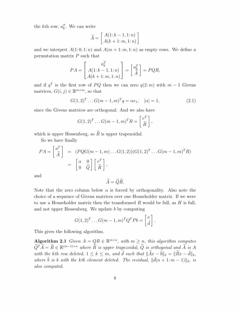
the kth row, aTk . We can write
A =
[A(1: k − 1, 1: n)
A(k + 1: m, 1: n)
]
and we interpret A(1: 0, 1: n) and A(m + 1: m, 1: n) as empty rows. We define a
permutation matrix P such that
PA =
aTk
A(1: k − 1, 1: n)
A(k + 1: m, 1: n)
=
[aT
k
A
]= PQR,
and if qT is the first row of PQ then we can zero q(2: m) with m − 1 Givens
matrices, G(i, j) ∈ Rm×m, so that
G(1, 2)T . . . G(m − 1, m)T q = αe1, |α| = 1, (2.1)
since the Givens matrices are orthogonal. And we also have
G(1, 2)T . . . G(m − 1, m)T R =
[vT
R
],
which is upper Hessenberg, so R is upper trapezoidal.
So we have finally
PA =
[aT
A
]= (PQG(m − 1, m) . . . G(1, 2))(G(1, 2)T . . . G(m − 1, m)TR)
=
[α 0
0 Q
] [vT
R
],
and
A = QR.
Note that the zero column below α is forced by orthogonality. Also note the
choice of a sequence of Givens matrices over one Householder matrix. If we were
to use a Householder matrix then the transformed R would be full, as H is full,
and not upper Hessenberg. We update b by computing
G(1, 2)T . . . G(m − 1, m)T QT Pb =
[ν
d
].
This gives the following algorithm.
Algorithm 2.1 Given A = QR ∈ Rm×n, with m ≥ n, this algorithm computes
QT A = R ∈ R(m−1)×n where R is upper trapezoidal, Q is orthogonal and A is A
with the kth row deleted, 1 ≤ k ≤ m, and d such that ‖Ax − b‖2 = ‖Rx − d‖2,
where b is b with the kth element deleted. The residual, ‖d(n + 1: m − 1)‖2, is
also computed.
8

qT = Q(k, 1: m)
if k 6= 1
% Permute b
b(2: k) = b(1: k − 1)
end
d = QT b
for j = m − 1:−1: 1
[c(j), s(j)] = givens(q(j), q(j + 1))
% Update q
q(j) = c(j)q(j) − s(j)q(j + 1)
% Update R if there is a nonzero row
if j ≤ n
R(j: j + 1, j: n) =
[c(j) s(j)
−s(j) c(j)
]T
R(j: j + 1, j: n)
end
% Update d
d(j: j + 1) =
[c(j) s(j)
−s(j) c(j)
]T
d(j: j + 1)
end
R = R(2: m, 1: n)
d = d(2: m)
% Compute the residual
resid = ‖d(n + 1: m − 1)‖2
Computing R requires 3n2 flops, versus 2n2(m − n/3) for the Householder
QR factorization of A. If Q is required, it can be computed with the following
algorithm.
Algorithm 2.2 Given vectors c and s from Algorithm 2.1 this algorithm forms
an orthogonal matrix Q ∈ R(m−1)×(m−1) such that A = QR, where A is the matrix
A = QR with the kth row deleted.
if k 6= 1
% Permute Q
Q(2: k, 1: m) = Q(1: k − 1, 1: m)
end
for j = m − 1:−1: 2
Q(2: m, j: j + 1) = Q(2: m, j: j + 1)
[c(j) s(j)
−s(j) c(j)
]
end
9

% Do not need to update 1st column of Q
Q(2: m, 2) = s(1)Q(2: m, 1) + c(1)Q(2: m, 2)
Q = Q(2: m, 2: m)
2.1.2 Deleting a Block of Rows
If a block of p observations is to be deleted from our least squares problem,
equivalent to deleting the p rows A(k: k + p − 1, 1: n) from A, we would like to
find an analogous method to Algorithm 2.1 that uses Householder matrices, such
that if H is a product of p Householder matrices then
PA =
[A(k: k + p − 1, 1: n)
A
]= (PQH)(HR) =
[I 0
0 Q
] [V
R
].
However as noted in the single row case, HR is full and H is chosen to introduce
zeros in Q not R. Thus in order to compute A = QR and d, we need the
equivalent of p steps of Algorithm 2.1 and Algorithm 2.2, since Givens matrices
only affect two rows of the matrix they are multiplying, and so we have the
following algorithm.
Algorithm 2.3 Given A = QR ∈ Rm×n, with m ≥ n, this algorithm computes
QT A = R ∈ R(m−p)×n where R is upper trapezoidal, Q is orthogonal and A is A
with the kth to (k + p − 1)st rows deleted, 1 ≤ k ≤ m − p + 1, 1 ≤ p < m, and
d such that ‖Ax − b‖2 = ‖Rx − d‖2, where b is b with the kth to (k + p − 1)st
elements deleted. The residual, ‖d(n + 1: m− p)‖2, is also computed.
W = Q(k: k + p − 1, 1: m)
if k 6= 1
% Permute b
b(p + 1: k + p − 1) = b(1: k − 1)
end
d = QT b
for i = 1: p
for j = m − 1:−1: i
[C(i, j), S(i, j)] = givens(W (i, j), W (i, j + 1))
% Update W
W (i, j) = W (i, j)C(i, j) − W (i, j + 1)S(i, j)
W (i + 1: p, j: j + 1) = W (i + 1: p, j: j + 1)
[C(i, j) S(i, j)
−S(i, j) C(i, j)
]
% Update R if there is a nonzero row
if j ≤ n + i − 1
10

R(j: j + 1, j − i + 1: n) =[C(i, j) S(i, j)
−S(i, j) C(i, j)
]T
R(j: j + 1, j − i + 1: n)
end
% Update d
d(j: j + 1) =
[C(i, j) S(i, j)
−S(i, j) C(i, j)
]T
d(j: j + 1)
end
end
R = R(p + 1: m, 1: n)
d = d(p + 1: m)
% Compute the residual
resid = ‖d(n + 1: m − p)‖2
Computing R requires 3n2p + p2(m/3− p) flops, versus 2n2(m− p− n/3) for
the Householder QR factorization of A. Note the following algorithm to compute
Q is more economical than calling Algorithm 2.2 p times, saving 3mp2 flops by
not updating the first p rows of Q.
Algorithm 2.4 Given matrices C and S from Algorithm 2.3 this algorithm
forms an orthogonal matrix Q ∈ R(m−p)×(m−p) such that A = QR, where A is
the matrix A = QR with the kth to (k + p − 1)st rows deleted.
if k 6= 1
% Permute Q
Q(p + 1: k + p − 1, 1: m) = Q(1: k − 1, 1: m)
end
for i = 1: p
for j = m − 1:−1: i + 1
Q(p + 1: m, j: j + 1) = Q(p + 1: m, j: j + 1)
[C(i, j) S(i, j)
−S(i, j) C(i, j)
]
end
end
% Do not need to update columns 1: p of Q
Q(p + 1: m, i + 1) = S(i, i)Q(p + 1: m, i) + C(i, i)Q(p + 1: m, i + 1)
Q = Q(p + 1: m, p + 1: m)
2.1.3 Updating the QR Factorization for any m and n
The relevant parts of Algorithm 2.3 and Algorithm 2.4 could be used to update
the QR factorization of A in the case when m < n without any alteration.
11

2.2 Alternative Methods for Deleting Rows
2.2.1 Hyperbolic Transformations
If we have the QR factorization A = QR ∈ Rm×n, then
AT A = RT QT QR = RT R,
which is a Cholesky factorization of AT A. And if we define a permutation matrix
P such that
PA =
aT
k
A(1: k − 1, 1: n)
A(k + 1: m, 1: n)
=
[aT
A
]= PQR,
where aTk is the kth row of A, then we have
RT QT P TPQR = RT R = AT A =
[aT
k
A
]T [aT
k
A
]. (2.2)
Thus if we find R, such that RT R = AT A, then we have computed R for A being A
with the kth row deleted. This can be achieved with hyperbolic transformations.
We define W ∈ Rm×m as pseudo-orthogonal with respect to the signature
matrix
J = diag(±1) ∈ Rm×m
if
W T JW = J.
If we transform a matrix with W we say that this is a hyperbolic transformation.
Now from (2.2) we have
AT A = AT A − akaTk
= RT R − akaTk
= [ RT ak ]
[In 0
0 −1
] [R
aTk
],
with the signature matrix
J =
[In 0
0 −1
]. (2.3)
And suppose there is a W ∈ R(n+1)×(n+1) such that W T JW = J with the property
W
[R
aTk
]=
[R
0
]
12

is upper trapezoidal. It follows that
AT A = [ RT ak ] W TJW
[R
aTk
]
= [ RT 0 ] J
[R
0
]
= RT R,
which is the Cholesky factorization we seek.
We construct the hyperbolic transformation matrix, W , by a product of hy-
perbolic rotations, W (i, n + 1) ∈ R(n+1)×(n+1), which are of the form
i n + 1
W (i, n + 1) =
I
c −s
I
−s c
i
n + 1
where c = cosh(θ) and s = sinh(θ) for some θ and c2 − s2 = 1. W (i, n +
1)T JW (i, n + 1) = J , where J is given in (2.3).
W (i, n + 1)x only transforms the ith and (n + 1)st elements. To solve the
2 × 2 problem [c −s
−s c
] [xi
xn+1
]=
[y
0
],
we note that cxn+1 = sxi and there is no solution for xi = xn+1 6= 0. If xi 6= xn+1
then we can compute c and s with the following algorithm.
Algorithm 2.5 This algorithm generates scalars c and s such that[c −s
−s c
] [x1
x2
]=
[y
0
]where x1, x2 and y are scalars and c2 − s2 = 1,
if a solution exists.
if x2 = 0
s = 0
c = 1
else
if |x2| < |x1|t = x2/x1
c = 1/√
1 − t2
s = ct
else
13

no solution exists
end
end
Note the norm of the rotation gets large as x1 gets close to x2.
We thus generate n hyperbolic transformations such that
W (n, n + 1) . . .W (2, n + 1)W (1, n + 1)
[R
aTk
]=
[R
0
].
It turns out that all the W (i, n + 1) can be found if A has full rank [1].
2.2.2 Chamber’s Algorithm
A method due to Chambers [5] mixes a hyperbolic and Givens rotation. If we
have our usual Givens transformation on the vector x[
c s
−s c
]T [x1
x2
],
then the transformed xi, xi, are
x1 = cx1 − sx2, (2.4)
x2 = sx1 + cx2,
with
c =x1√
x21 + x2
2
, s =−x2√x2
1 + x22
.
Now suppose we know x1 and want to recreate the vector x, then rearrang-
ing (2.4) we have
x1 = (sx2 + x1)/c,
x2 = sx1 + cx2,
with
c =
√x2
1 − x22
x1, s =
−x2
x1.
Thus we can recreate the steps that would have updated R had we added aTk
to A, instead of deleting it from A. At the ith step, for i = 1: n + 1, with
x1 = R(i, i),
x1 = R(i, i),
x2 = a(i−1)k (i),
14

we compute, for j = i: n + 1:
R(i, j) = (R(i, i) + sak(j))/c,
a(i)k (j) = sR(i, j) + ca
(i−1)k (j).
2.2.3 Saunders’ Algorithm
If Q is not available then Saunders’ algorithm [17] offers an alternative to Algo-
rithm 2.1. The first row of
PA =
[aT
k
A
]= PQ
[R1
0
],
can be written
aTk = qT
[R1
0
]= [ qT
1 qT2 ]
[R1
0
],
where q1 ∈ Rn. We compute q1 by solving
RT1 q1 = ak,
and since ‖q‖2 = 1 we have
η = ‖q2‖2 = (1 − ‖q1‖22)
1/2.
Then we have, with the same Givens matrices in (2.1),
G(n + 1, n + 2)T . . . G(m − 1, m)T
[q1
q2
]=
q1
±η
0
,
which would not effect R. So we need only compute
G(1, 2)T . . . G(n, n + 1)T
[q1
η
]= αe1, |α| = 1,
and update R by
G(1, 2)T . . . G(n, n + 1)T R =
[vT
R
].
This algorithm is implemented in LINPACK’s xCHDD.
15

2.2.4 Stability Issues
Stewart [20] shows that hyperbolic transformations are not backward stable.
However, Chamber’s and Saunder’s algorithms are relationally stable [3], [19],
that is if W represents the product of all the transformations then
W TR =
[vT
R
]+ E,
where
‖E‖ ≤ cnu‖R‖,
and cn is a constant that depends on n.
Saunder’s algorithm can fail for certain data, see [2].
2.2.5 Block Downdating
Hyperbolic transformations have been generalized by Rader and Steinhardt as
hyperbolic Householder transformations [15].
Alternatives are discussed in Elden and Park [8], and the references contained
within, including a generalization of Saunders Algorithm. See also Bojanczyk,
Higham and Patel [4] and Olskanskyj, Lebak and Bojanczyk [13].
2.3 Adding Rows
2.3.1 Adding One Row
If we wish to add an observation to our least squares problem then we need to
add a row, uT ∈ Rn, in the kth position, k = 1: m + 1, of A = QR ∈ R
m×n,
m ≥ n. We can then write
A =
A(1: k − 1, 1: n)
uT
A(k: m, 1: n)
and we can define a permutation matrix, P , such that
PA =
[A
uT
],
and then [QT 0
0 1
]PA =
[R
uT
]. (2.5)
16
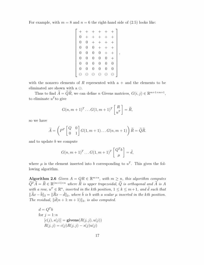
For example, with m = 8 and n = 6 the right-hand side of (2.5) looks like:
+ + + + + +
0 + + + + +
0 0 + + + +
0 0 0 + + +
0 0 0 0 + +
0 0 0 0 0 +
0 0 0 0 0 0
0 0 0 0 0 0
⊖ ⊖ ⊖ ⊖ ⊖ ⊖
,
with the nonzero elements of R represented with a + and the elements to be
eliminated are shown with a ⊖.
Thus to find A = QR, we can define n Givens matrices, G(i, j) ∈ Rm+1×m+1,
to eliminate uT to give
G(n, m + 1)T . . . G(1, m + 1)T
[R
uT
]= R,
so we have
A =
(P T
[Q 0
0 1
]G(1, m + 1) . . .G(n, m + 1)
)R = QR.
and to update b we compute
G(n, m + 1)T . . . G(1, m + 1)T
[QT b
µ
]= d,
where µ is the element inserted into b corresponding to uT . This gives the fol-
lowing algorithm.
Algorithm 2.6 Given A = QR ∈ Rm×n, with m ≥ n, this algorithm computes
QT A = R ∈ R(m+1)×n where R is upper trapezoidal, Q is orthogonal and A is A
with a row, uT ∈ Rn, inserted in the kth position, 1 ≤ k ≤ m+1, and d such that
‖Ax− b‖2 = ‖Rx− d‖2, where b is b with a scalar µ inserted in the kth position.
The residual, ‖d(n + 1: m + 1)‖2, is also computed.
d = QT b
for j = 1: n
[c(j), s(j)] = givens(R(j, j), u(j))
R(j, j) = c(j)R(j, j) − s(j)u(j)
17

% Update jth row of R and u
t1 = R(j, j + 1: n)
t2 = u(j + 1: n)
R(j, j + 1: n) = c(j)t1 − s(j)t2
u(j + 1: n) = s(j)t1 + c(j)t2
% Update jth row of d and µ
t1 = d(j)
t2 = µ
d(j) = c(j)t1 − s(j)t2
µ = s(j)t1 + c(j)t2
end
R =
[R
0
]
d =
[d
µ
]
% Compute the residual
resid = ‖d(n + 1: m + 1)‖2
Computing R requires 3n2 flops, versus 2n2(m − n/3) for the Householder
QR factorization of A. If Q is required, it can be computed with the following
algorithm.
Algorithm 2.7 Given vectors c and s from Algorithm 2.6 this algorithm forms
an orthogonal matrix Q ∈ R(m+1)×(m+1) such that A = QR, where A is the matrix
A = QR with a row added in the kth position.
Set Q =
[Q 0
0 1
]
if k 6= m + 1
% Permute Q
Q =
Q(1: k − 1, 1: n)
Q(m + 1, 1: n)
Q(k: m, 1: n)
end
for j = 1: n
t1 = Q(1: m + 1, j)
t2 = Q(1: m + 1, m + 1)
Q(1: m + 1, j) = c(j)t1 − s(j)t2
Q(1: m + 1, m + 1) = s(j)t1 + c(j)t2
end
18

2.3.2 Adding a Block of Rows
To add a block of p observations to our least squares problem we add a block
of p rows, U ∈ R(p×n), in the kth to (k + p − 1)st positions, k = 1: m + 1, of
A = QR ∈ Rm×n, m ≥ n, we can then write
A =
A(1: k − 1, 1: n)
U
A(k: m, 1: n)
and we can define a permutation matrix, P , such that
PA =
[A
U
],
and [QT 0
0 Ip
]PA =
[R
U
]. (2.6)
For example, with m = 8, n = 6 and p = 3 the right-hand side of Equation (2.6)
looks like:
+ + + + + +
0 + + + + +
0 0 + + + +
0 0 0 + + +
0 0 0 0 + +
0 0 0 0 0 +
0 0 0 0 0 0
0 0 0 0 0 0
⊖ ⊖ ⊖ ⊖ ⊖ ⊖⊖ ⊖ ⊖ ⊖ ⊖ ⊖⊖ ⊖ ⊖ ⊖ ⊖ ⊖
,
with the nonzero elements of R represented with a + and the elements to be
eliminated are shown with a ⊖.
Thus to find A = QR, we can define n Householder matrices to eliminate U
to give
Hn . . .H1
[R
U
]= R,
so we have
A =
(P T
[Q 0
0 Ip
]H1 . . .Hn
)R = QR.
19

The Householder matrix, Hj ∈ R(m+p)×(m+p), will zero the jth column of U .
Its associated Householder vector, vj ∈ R(m+p), is such that
vj(1: j − 1) = 0,
vj(j) = 1,
vj(j + 1: m) = 0,
vj(m + 1: m + p) = x/(rjj − ‖ [ rjj xT ] ‖2), where x = U(1: p, j).
(2.7)
So the Hj have the following structure
Hj =
I
hjj [ hj,m+1 . . . hj,m+p ]
I
hm+1,j...
hm+p,j
hm+1,m+1 . . . hm+1,m+p...
...
hm+p,m+1 . . . hm+p,m+p
.
Then to update b we compute
Hn . . .H1
[QT b
e
]= d,
where e is such that Ux = e. This gives the following algorithm.
Algorithm 2.8 Given A = QR ∈ Rm×n, with m ≥ n, this algorithm computes
QT A = R ∈ R(m+p)×n where R is upper trapezoidal, Q is orthogonal and A is A
with a block of rows, U ∈ Rp×n, inserted in the kth to (k + p − 1)st positions,
1 ≤ k ≤ m + 1, p ≥ 1, and d such that ‖Ax − b‖2 = ‖Rx − d‖2, where b is
b with the vector e inserted in the kth to (k + p − 1)st positions. The residual,
‖d(n + 1: m + p)‖2, is also computed.
d = QT b
for j = 1: n
[V (1: p, j), τ(j)] = householder(R(j, j), U(1: p, j))
% Remember old jth row of R
Rj = R(j, j + 1: n)
% Update jth row of R
R(j, j: n) = (1 − τ(j))R(j, j: n) − τ(j)V (1: p, j)TU(1: p, j: n)
% Update trailing part if U
if j < n
20

U(1: p, j + 1: n) = U(1: p, j + 1: n) − τ(j)V (1: p, j)Rj
−τ(j)V (1: p, j)(V (1: p, j)TU(1: p, j + 1: n))
end
% Remember old jth element of d
dj = R(j)
% Update jth element of d
d(j) = (1 − τ(j))d(j) − τ(j)V (1: p, j)Te(1: p)
% Update e
e(1: p) = e(1: p) − τ(j)V (1: p, j)dj
−τ(j)V (1: p, j)(V (1: p, j)Te(1: p))
end
R =
[R
0
]
d =
[d
e
]
% Compute the residual
resid = ‖d(n + 1: m + p)‖2
Computing R requires 2n2p flops, versus 2n2(m+p−n/3) for the Householder
QR factorization of A. If Q is required, it can be computed with the following
algorithm.
Algorithm 2.9 Given the matrix V and vector τ from Algorithm 2.8 this algo-
rithm forms an orthogonal matrix Q ∈ R(m+p)×(m+p) such that A = QR, where A
is the matrix A = QR with a block of rows inserted in the kth to (k + p − 1)st
positions.
Set Q =
[Q 0
0 I
]
if k 6= m + 1
% Permute Q
Q =
Q(1: k − 1, 1: m + p)
Q(m + 1: m + p, 1: m + p)
Q(k: m, 1: m + p)
end
for j = 1: n
% Remember jth column of Q
Qk = Q(1: m + p, j)
% Update jth column
Q(1: m + p, j) = Q(1: m + p, j)(1 − τ(j))−Q(1: m + p, m + 1: m + p)τ(j)V (1: p, j)
21

% Update m + 1: p columns of Q
Q(1: m + p, m + 1: m + p) = Q(1: m + p, m + 1: m + p)
−τ(j)QkV (1: p, j)T
−τ(j)(Q(1: m + p, m + 1: m + p)V (1: p, j))V (1: p, j)T
end
This algorithm could be made more economical by noting that at the jth
stage, for i > m, qij = 0, and avoiding some unnecessary multiplications by zero.
Also Q(m + 1: m + p, 1: m) = 0 and Q(m + 1: m + p, m + 1: m + p) = Ip, prior to
the permutation.
Algorithm 2.8 can be improved by exploiting the Level 3 BLAS by using the
representation of the product of nb Householder matrices, Hi, as
H1H2 . . . Hnb= I − V TV T , (2.8)
where
V = [ v1 v2 . . . vnb] =
[V1
V2
],
and V1 ∈ Rnb×nb is lower triangular and T is upper triangular. We can write
QT A =
R11 R12 R13
0 R22 R23
0 0 R33
0 0 0
U11 U12 U13
, (2.9)
where the Rii are upper triangular with R11 ∈ Rr×r and R22 ∈ R
nb×nb, and after
we have updated the first r columns, then the transformed right-hand side of
(2.9) looks like:
R(r)11 R
(r)12 R
(r)13
0 R(r)22 R
(r)23
0 0 R(r)33
0 0 0
0 U(r)12 U
(r)13
.
Now we eliminate the first column of U(r)12 and instead of updating the trailing
parts of R and U we update only the trailing parts of U(r)12 and the (r + 1)st
row of R(r)22 , which are the only elements affected in this middle block column,
and continue in this way until U12 has been eliminated. We can then employ the
representation (2.8) to apply nb Householder matrices to update the last block
column in one go. We have, by the definition of the Householder vectors in (2.7)
V =
[V1
V2
], V1 = Inb
, V2 =
[0
V 2
],
22

where V 2 ∈ Rp×nb hold the essential part of the Householder vectors for the
current block column. Then
[ I − V T T V T ]T
R23
R33
0
U13
=
Im+p−r −
Inb
0
0
V 2
T T [ Inb
0 0 VT
2 ]
R23
R33
0
U13
=
(Inb− T T )R23 − T T V
T
2 U13
R33
0
−V 2TT R23 + (I − V 2T
T VT
2 )U13
,
This approach leads to a blocked algorithm, where at the kth stage we fac-
torize [ RT22 0 UT
12 ]T , where R22 ∈ Rnb×nb and U12 ∈ R
p×nb, then update
R23 ∈ Rnb×(n−knb) and UT
13 ∈ Rp×(n−knb) as above. And to update QT b = d
we compute
d(1: (k − 1)nb)
(Inb− T T )d((k − 1)nb + 1: knb) − T T V
T
2 e
d(knb + 1: m)
−V 2TT d((k − 1)nb + 1: knb) + (I − V 2T
T VT
2 )e
=
[d
e
].
Algorithm 2.10 Given A = QR ∈ Rm×n, with m ≥ n, this algorithm computes
QT A = R ∈ R(m+p)×n where R is upper trapezoidal, Q is orthogonal and A is A
with a block of rows, U ∈ Rp×n, inserted in the kth to (k + p − 1)st positions,
1 ≤ k ≤ m + 1, p ≥ 1, and d such that ‖Ax − b‖2 = ‖Rx − d‖2, where b is
b with the vector e inserted in the kth to (k + p − 1)st positions. The residual,
‖d(n+1: m+p)‖2, is also computed. This is a Level 3 BLAS algorithm with block
size nb.
d = QT b
for k = 1: nb: n
% Check for the last column block
jb = min(nb, n − k + 1)
Factorize current block with Algorithm 2.8 where
V is V (1: p, k: k + jb − 1)
% If we are not in last block column build T
% and update trailing matrix
if k + jb ≤ n
for j = k: k + jb − 1
% Build T
23

if j = k
T (1, 1) = τ(j)
else
T (1: j − k, j − k + 1) = −τ(j)T (1: j − k, 1: j − k)
∗V (1: p, k: j − 1)T V (1: p, j)
T (j − k + 1, j − k + 1) = τ(j)
end
end
% Compute products we use more than once
TV = T T V (1: p, k: k + jb − 1)T
Te = TV e
TU = TV U(1: p, , k + jb: n)
% Remember old d and e
dk = d(k: k + jb − 1)
ek = e
% Update d and e
d(k: k + jb − 1) = dk − T T dk − Te
e = −V (1: p, k: k + jb − 1)T T dk + ek
−V (1: p, k: k + jb − 1)Te
% Remember old trailing parts of R and U
Rk = R(k: k + jb − 1, k + jb: n)
Uk = U(1: p, k + jb: n)
% Update trailing parts of R and U
R(k: k + jb − 1, k + jb: n) = Rk − T TRk − TU
U(1: p, k + jb: n) = −V (1: p, k: k + jb − 1)T T Rk + Uk
−V (1: p, k: k + jb − 1)TU
end
end
R =
[R
0
]
d =
[d
e
]
% Compute the residual
resid = ‖d(n + 1: m + p)‖2
We could apply the same approach to improve Algorithm 2.9.
24
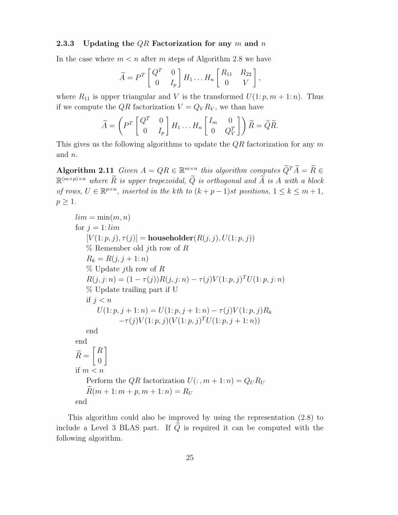
2.3.3 Updating the QR Factorization for any m and n
In the case where m < n after m steps of Algorithm 2.8 we have
A = P T
[QT 0
0 Ip
]H1 . . .Hn
[R11 R22
0 V
],
where R11 is upper triangular and V is the transformed U(1: p, m + 1: n). Thus
if we compute the QR factorization V = QV RV , we than have
A =
(P T
[QT 0
0 Ip
]H1 . . .Hn
[Im 0
0 QTV
])R = QR.
This gives us the following algorithms to update the QR factorization for any m
and n.
Algorithm 2.11 Given A = QR ∈ Rm×n this algorithm computes QT A = R ∈
R(m+p)×n where R is upper trapezoidal, Q is orthogonal and A is A with a block
of rows, U ∈ Rp×n, inserted in the kth to (k + p− 1)st positions, 1 ≤ k ≤ m + 1,
p ≥ 1.
lim = min(m, n)
for j = 1: lim
[V (1: p, j), τ(j)] = householder(R(j, j), U(1: p, j))
% Remember old jth row of R
Rk = R(j, j + 1: n)
% Update jth row of R
R(j, j: n) = (1 − τ(j))R(j, j: n) − τ(j)V (1: p, j)TU(1: p, j: n)
% Update trailing part if U
if j < n
U(1: p, j + 1: n) = U(1: p, j + 1: n) − τ(j)V (1: p, j)Rk
−τ(j)V (1: p, j)(V (1: p, j)TU(1: p, j + 1: n))
end
end
R =
[R
0
]
if m < n
Perform the QR factorization U(: , m + 1: n) = QURU
R(m + 1: m + p, m + 1: n) = RU
end
This algorithm could also be improved by using the representation (2.8) to
include a Level 3 BLAS part. If Q is required it can be computed with the
following algorithm.
25
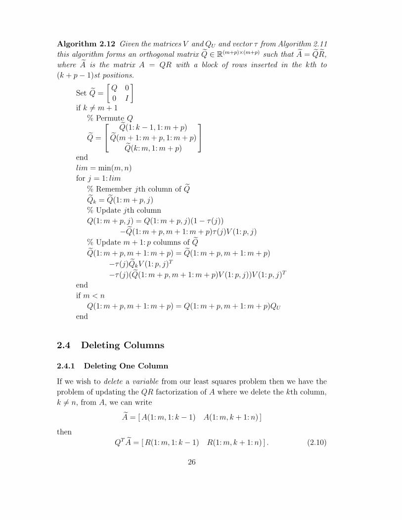
Algorithm 2.12 Given the matrices V and QU and vector τ from Algorithm 2.11
this algorithm forms an orthogonal matrix Q ∈ R(m+p)×(m+p) such that A = QR,
where A is the matrix A = QR with a block of rows inserted in the kth to
(k + p − 1)st positions.
Set Q =
[Q 0
0 I
]
if k 6= m + 1
% Permute Q
Q =
Q(1: k − 1, 1: m + p)
Q(m + 1: m + p, 1: m + p)
Q(k: m, 1: m + p)
end
lim = min(m, n)
for j = 1: lim
% Remember jth column of Q
Qk = Q(1: m + p, j)
% Update jth column
Q(1: m + p, j) = Q(1: m + p, j)(1 − τ(j))
−Q(1: m + p, m + 1: m + p)τ(j)V (1: p, j)
% Update m + 1: p columns of Q
Q(1: m + p, m + 1: m + p) = Q(1: m + p, m + 1: m + p)
−τ(j)QkV (1: p, j)T
−τ(j)(Q(1: m + p, m + 1: m + p)V (1: p, j))V (1: p, j)T
end
if m < n
Q(1: m + p, m + 1: m + p) = Q(1: m + p, m + 1: m + p)QU
end
2.4 Deleting Columns
2.4.1 Deleting One Column
If we wish to delete a variable from our least squares problem then we have the
problem of updating the QR factorization of A where we delete the kth column,
k 6= n, from A, we can write
A = [ A(1: m, 1: k − 1) A(1: m, k + 1: n) ]
then
QT A = [R(1: m, 1: k − 1) R(1: m, k + 1: n) ] . (2.10)
26
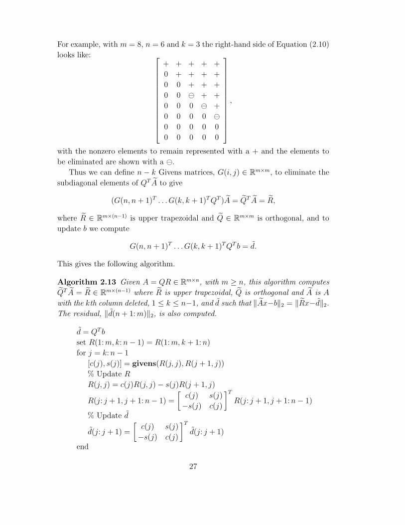
For example, with m = 8, n = 6 and k = 3 the right-hand side of Equation (2.10)
looks like:
+ + + + +
0 + + + +
0 0 + + +
0 0 ⊖ + +
0 0 0 ⊖ +
0 0 0 0 ⊖0 0 0 0 0
0 0 0 0 0
,
with the nonzero elements to remain represented with a + and the elements to
be eliminated are shown with a ⊖.
Thus we can define n − k Givens matrices, G(i, j) ∈ Rm×m, to eliminate the
subdiagonal elements of QT A to give
(G(n, n + 1)T . . . G(k, k + 1)T QT )A = QT A = R,
where R ∈ Rm×(n−1) is upper trapezoidal and Q ∈ R
m×m is orthogonal, and to
update b we compute
G(n, n + 1)T . . . G(k, k + 1)TQT b = d.
This gives the following algorithm.
Algorithm 2.13 Given A = QR ∈ Rm×n, with m ≥ n, this algorithm computes
QT A = R ∈ Rm×(n−1) where R is upper trapezoidal, Q is orthogonal and A is A
with the kth column deleted, 1 ≤ k ≤ n−1, and d such that ‖Ax−b‖2 = ‖Rx−d‖2.
The residual, ‖d(n + 1: m)‖2, is also computed.
d = QT b
set R(1: m, k: n − 1) = R(1: m, k + 1: n)
for j = k: n − 1
[c(j), s(j)] = givens(R(j, j), R(j + 1, j))
% Update R
R(j, j) = c(j)R(j, j) − s(j)R(j + 1, j)
R(j: j + 1, j + 1: n − 1) =
[c(j) s(j)
−s(j) c(j)
]T
R(j: j + 1, j + 1: n − 1)
% Update d
d(j: j + 1) =
[c(j) s(j)
−s(j) c(j)
]T
d(j: j + 1)
end
27

R = upper triangular part of R(1: m, 1: n − 1)
% Compute the residual
resid = ‖d(n + 1: m)‖2
Computing R requires n2/2 − nk + k2/2 flops, versus 2n2(m − n/3) for the
Householder QR factorization of A. If Q is required, it can be computed with
the following algorithm.
Algorithm 2.14 Given vectors c and s from Algorithm 2.13 this algorithm forms
an orthogonal matrix Q ∈ Rm×m such that A = QR, where A is the matrix
A = QR with the kth column deleted.
for j = k: n − 1
Q(1: m, j: j + 1) = Q(1: m, j: j + 1)
[c(j) s(j)
−s(j) c(j)
]
end
Q = Q
In the case when k = n then
A = A(1: m, 1: k − 1), R = R(1: m, 1: k − 1), Q = Q, and d = QT b,
and there is no computation to do.
2.4.2 Deleting a Block of Columns
To delete a block of p variables from our least squares problem we delete a block
of p columns, from the kth column onwards, from A and we can write
A = [ A(1: m, 1: k − 1) A(1: m, k + p: n) ]
then
QT A = [ R(1: m, 1: k − 1) R(1: m, k + p: n) ] . (2.11)
For example, with m = 10, n = 8, k = 3 and p = 3 the right-hand side of
Equation (2.11) looks like:
28

+ + + + +
0 + + + +
0 0 + + +
0 0 ⊖ + +
0 0 ⊖ ⊖ +
0 0 ⊖ ⊖ ⊖0 0 0 ⊖ ⊖0 0 0 0 ⊖0 0 0 0 0
0 0 0 0 0
,
with the nonzero elements to remain represented with a + and the elements to
be eliminated are shown with a ⊖.
Thus we can define n − p − k + 1 Householder matrices, Hj ∈ Rm×m, with
associated Householder vectors, vj ∈ R(p+1) such that
vj(1: j − 1) = 0,
vj(j) = 1,
vj(j + 1: j + p) = x/((QT A)jj − ‖ [ (QT A)jj xT ] ‖2),
where x = QT A(j + 1: j + p, j),
vj(j + p + 1: m) = 0.
The Hj have the following structure
Hj =
I
hj,j . . . hj,j+p...
...
hj+p,j . . . hj+p,j+p
I
,
and can be used to eliminate the subdiagonal of QT A to give
(Hn−p . . .HkQT )A = QT A = R,
where R ∈ Rm×(n−p) is upper trapezoidal and Q ∈ R
m×m is orthogonal, and we
update b by computing
Hn−p . . .HkQT b = d.
This gives the following algorithm.
29

Algorithm 2.15 Given A = QR ∈ Rm×n, with m ≥ n, this algorithm computes
QT A = R ∈ Rm×(n−p) where R is upper trapezoidal, Q is orthogonal and A is A
with the kth to (k + p − 1)st columns deleted, 1 ≤ k ≤ n − p, 1 ≤ p < n, and d
such that ‖Ax− b‖2 = ‖Rx− d‖2. The residual, ‖d(n+1: m)‖2, is also computed.
d = QT b
set R(1: m, k: n − p) = R(1: m, k + p: n)
for j = k: n − p
[V (1: p, j), τ(j)] = householder(R(j, j), R(j + 1: j + p, j))
% Update R
R(j, j) = R(j, j) − τ(j)R(j, j) − τ(j)V (1: p, j)TR(j + 1: j + p, j)
if j < n − p
R(j: j + p, j + 1: n − p) = R(j: j + p, j + 1: n − p)
−τ(j)
[1
V (1: p, j)
]([ 1 V (1: p, j)T ]R(j: j + p, j + 1: n − p))
end
% Update d
d(j: j + p) = d(j: j + p, j + 1)
−τ(j)
[1
V (1: p, j)
]([ 1 V (1: p, j)T ] d(j: j + p))
end
R = upper triangular part of R(1: m, 1: n − p)
% Compute the residual
resid = ‖d(n + 1: m)‖2
Computing R requires 4(np(n/2 − p − k) + p2(p/2 + k) + pk2 flops, versus
2(n − p)2(m − (n − p)/3) for the Householder QR factorization of A. If Q is
required, it can be computed with the following algorithm.
Algorithm 2.16 Given the matrix V and vector τ from Algorithm 2.15 this
algorithm forms an orthogonal matrix Q ∈ Rm×m such that A = QR, where A is
the matrix A = QR with the kth to (k + p − 1)st columns deleted.
for j = k: n − p
Q(1: m, j: j + p) = Q(1: m, j: j + p)
−τ(j)(Q(1: m, j: j + p)
[1
V (1: p, j)
])[ 1 V (1: p, j)T ]
end
Q = Q
30

In the case when k = n − p + 1 then
A = A(1: m, 1: k − 1), R = R(1: m, 1: k − 1), Q = Q, and d = QT b,
and there is no computation to do.
2.4.3 Updating the QR Factorization for any m and n
In the case when m < n we need to:
• Increase the number of steps, we introduce lim, the last column to be
updated.
• Determine the last index of the Householder vectors, which cannot exceed
m.
This gives the following algorithms to update the QR factorization for any m and
n.
Algorithm 2.17 Given A = QR ∈ Rm×n this algorithm computes QT A = R ∈
Rm×(n−p) where R is upper trapezoidal, Q is orthogonal and A is A with the kth
to (k + p − 1)st columns deleted, 1 ≤ k ≤ min(m − 1, n − p), 1 ≤ p < n.
set R(1: m, k: n − p) = R(1: m, k + p: n)
lim = min(m − 1, n − p)
for j = k: lim
last = min(j + p, m)
[V (1: last − j, j), τ(j)] = householder(R(j, j), R(j + 1: last, j))
% Update R
R(j, j) = R(j, j) − τ(j)R(j, j) − τ(j)V (1: last − j, j)T R(j + 1: last, j)
if j < n − p
R(j: last, j + 1: n − p) = R(j: last, j + 1: n − p)
−τ(j)
[1
V (1: last − j, j)
]
∗ ([ 1 V (1: last − j, j)T ] R(j: last, j + 1: n − p))
end
end
R = upper triangular part of R(1: m, 1: n − p)
If Q is required, it can be computed with the following algorithm.
31
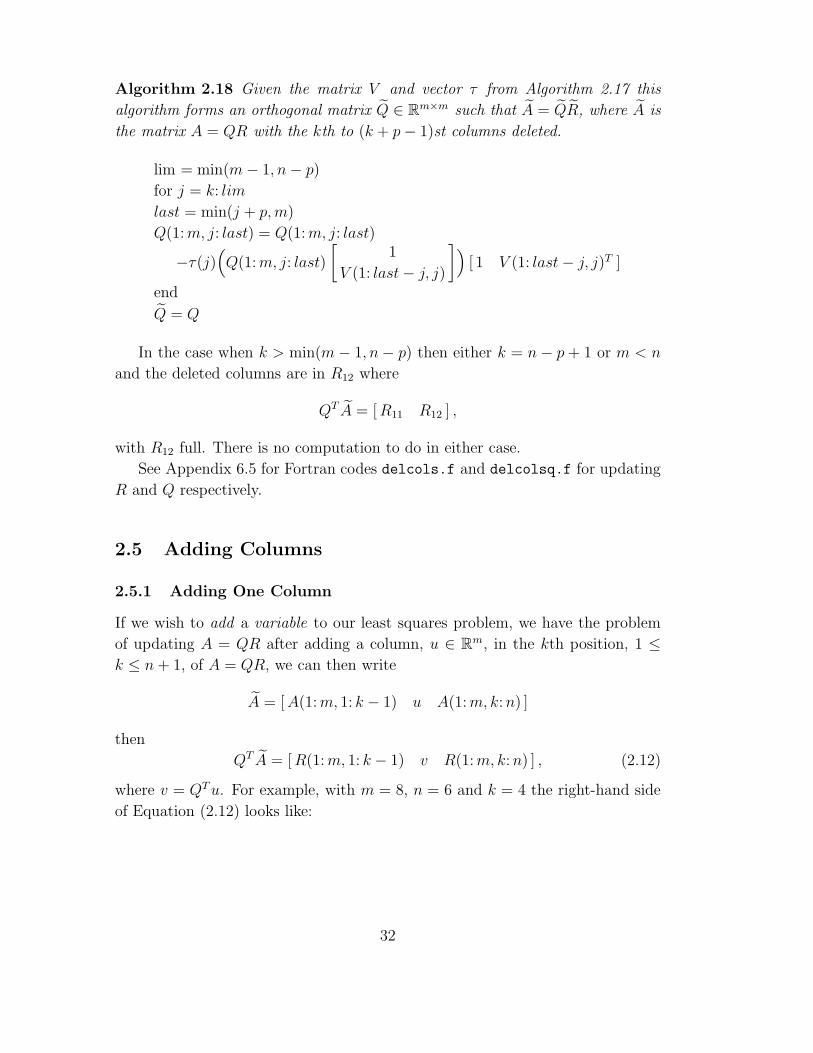
Algorithm 2.18 Given the matrix V and vector τ from Algorithm 2.17 this
algorithm forms an orthogonal matrix Q ∈ Rm×m such that A = QR, where A is
the matrix A = QR with the kth to (k + p − 1)st columns deleted.
lim = min(m − 1, n − p)
for j = k: lim
last = min(j + p, m)
Q(1: m, j: last) = Q(1: m, j: last)
−τ(j)(Q(1: m, j: last)
[1
V (1: last − j, j)
])[ 1 V (1: last − j, j)T ]
end
Q = Q
In the case when k > min(m − 1, n − p) then either k = n − p + 1 or m < n
and the deleted columns are in R12 where
QT A = [ R11 R12 ] ,
with R12 full. There is no computation to do in either case.
See Appendix 6.5 for Fortran codes delcols.f and delcolsq.f for updating
R and Q respectively.
2.5 Adding Columns
2.5.1 Adding One Column
If we wish to add a variable to our least squares problem, we have the problem
of updating A = QR after adding a column, u ∈ Rm, in the kth position, 1 ≤
k ≤ n + 1, of A = QR, we can then write
A = [ A(1: m, 1: k − 1) u A(1: m, k: n) ]
then
QT A = [ R(1: m, 1: k − 1) v R(1: m, k: n) ] , (2.12)
where v = QT u. For example, with m = 8, n = 6 and k = 4 the right-hand side
of Equation (2.12) looks like:
32

+ + + + + + +
0 + + + + + +
0 0 + + + + +
0 0 0 + + + +
0 0 0 ⊖ ⊕ + +
0 0 0 ⊖ 0 ⊕ +
0 0 0 ⊖ 0 0 ⊕0 0 0 ⊖ 0 0 0
,
with the nonzero elements to remain represented with a +, the elements to be
eliminated are ⊖ and the zero elements that can be filled in are shown with a ⊕.
Thus we can define m − k Givens matrices, G(i, j) ∈ Rm×m, to eliminate
v(k + 1: m). We then have
(G(k, k + 1)T . . . G(m − 1, m)T QT )A = QT A = R,
where R ∈ Rm×(n+1) is upper trapezoidal and Q ∈ R
m×m is orthogonal. We then
update b by computing
G(k, k + 1)T . . . G(m − 1, m)T QT b = d.
This gives the following algorithm.
Algorithm 2.19 Given A = QR ∈ Rm×n, with m ≥ n, this algorithm computes
QT A = R ∈ Rm×(n+1) where R is upper trapezoidal, Q is orthogonal and A is A
with a, u ∈ Rn, column inserted in the kth position, 1 ≤ k ≤ n + 1, and d such
that ‖Ax − b‖2 = ‖Rx − d‖2. The residual, ‖d(n + 1: m)‖2, is also computed.
u = QT u
d = QT b
for i = m:−1: k + 1
[c(i), s(i)] = givens(u(i − 1), u(i))
u(i − 1) = c(i)u(i − 1) − s(i)R(i)
% Update R if there is a nonzero row
if i ≤ n + 1
R(i − 1: i, i− 1: n) =
[c(i) s(i)
−s(i) c(i)
]T
R(i − 1: i, i − 1: n)
end
% Update R
33
d(i − 1: i) =
[c(i) s(i)
−s(i) c(i)
]T
d(i − 1: i)
end
if k = 1
R = upper triangular part of [ u R ]
else if k = n + 1
R = upper triangular part of [ R u ]
else
R = upper triangular part of [ R(1: m, 1: k − 1) u R(1: m, k: n) ]
end
% Compute the residual
resid = ‖d(n + 1: m)‖2
If Q is required, it can be computed with the following algorithm.
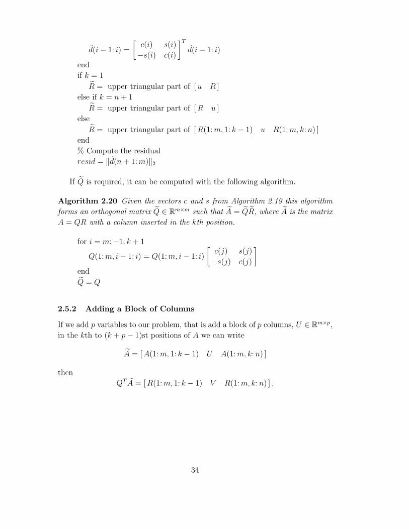
Algorithm 2.20 Given the vectors c and s from Algorithm 2.19 this algorithm
forms an orthogonal matrix Q ∈ Rm×m such that A = QR, where A is the matrix
A = QR with a column inserted in the kth position.
for i = m:−1: k + 1
Q(1: m, i − 1: i) = Q(1: m, i − 1: i)
[c(j) s(j)
−s(j) c(j)
]
end
Q = Q
2.5.2 Adding a Block of Columns
If we add p variables to our problem, that is add a block of p columns, U ∈ Rm×p,
in the kth to (k + p − 1)st positions of A we can write
A = [A(1: m, 1: k − 1) U A(1: m, k: n) ]
then
QT A = [ R(1: m, 1: k − 1) V R(1: m, k: n) ] ,
34
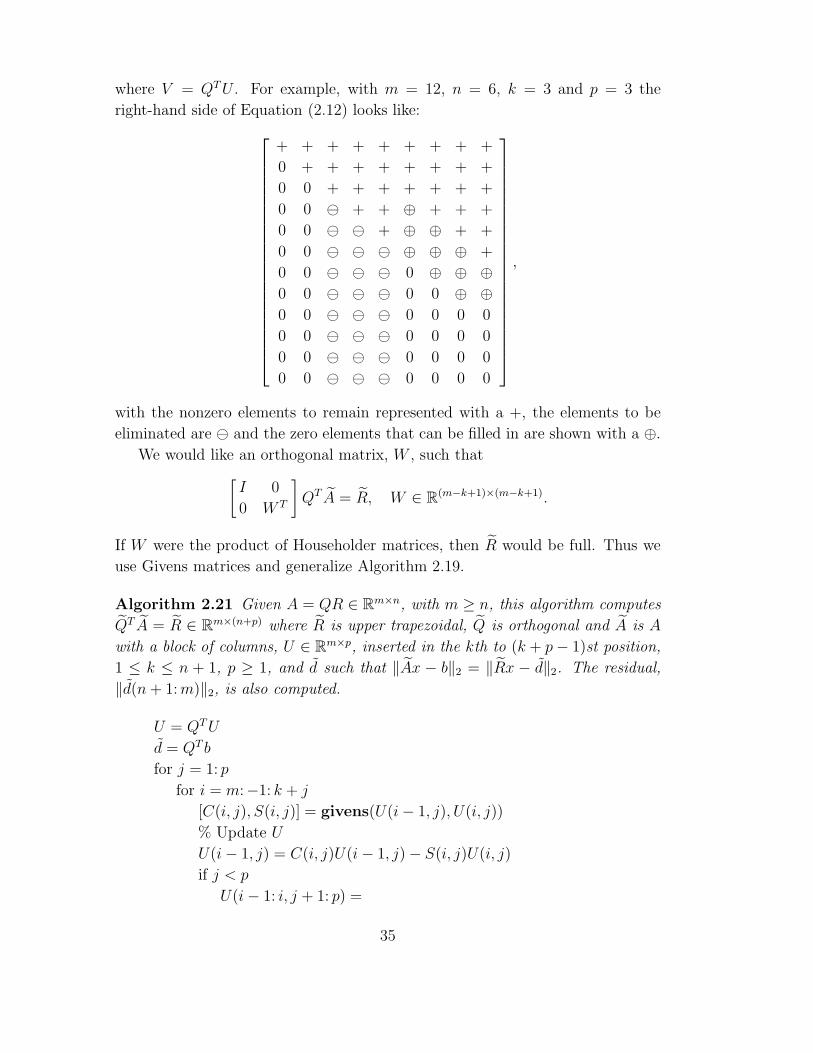
where V = QT U . For example, with m = 12, n = 6, k = 3 and p = 3 the
right-hand side of Equation (2.12) looks like:
+ + + + + + + + +
0 + + + + + + + +
0 0 + + + + + + +
0 0 ⊖ + + ⊕ + + +
0 0 ⊖ ⊖ + ⊕ ⊕ + +
0 0 ⊖ ⊖ ⊖ ⊕ ⊕ ⊕ +
0 0 ⊖ ⊖ ⊖ 0 ⊕ ⊕ ⊕0 0 ⊖ ⊖ ⊖ 0 0 ⊕ ⊕0 0 ⊖ ⊖ ⊖ 0 0 0 0
0 0 ⊖ ⊖ ⊖ 0 0 0 0
0 0 ⊖ ⊖ ⊖ 0 0 0 0
0 0 ⊖ ⊖ ⊖ 0 0 0 0
,
with the nonzero elements to remain represented with a +, the elements to be
eliminated are ⊖ and the zero elements that can be filled in are shown with a ⊕.
We would like an orthogonal matrix, W , such that
[I 0
0 W T
]QT A = R, W ∈ R
(m−k+1)×(m−k+1).
If W were the product of Householder matrices, then R would be full. Thus we
use Givens matrices and generalize Algorithm 2.19.
Algorithm 2.21 Given A = QR ∈ Rm×n, with m ≥ n, this algorithm computes
QT A = R ∈ Rm×(n+p) where R is upper trapezoidal, Q is orthogonal and A is A
with a block of columns, U ∈ Rm×p, inserted in the kth to (k + p − 1)st position,
1 ≤ k ≤ n + 1, p ≥ 1, and d such that ‖Ax − b‖2 = ‖Rx − d‖2. The residual,
‖d(n + 1: m)‖2, is also computed.
U = QT U
d = QT b
for j = 1: p
for i = m:−1: k + j
[C(i, j), S(i, j)] = givens(U(i − 1, j), U(i, j))
% Update U
U(i − 1, j) = C(i, j)U(i − 1, j) − S(i, j)U(i, j)
if j < p
U(i − 1: i, j + 1: p) =
35

[C(i, j) S(i, j)
−S(i, j) C(i, j)
]T
U(i − 1: i, j + 1: p)
end
% Update R if there is a nonzero row
if i ≤ n + j
R(i − 1: i, i − j: n) =[C(i, j) S(i, j)
−S(i, j) C(i, j)
]T
R(i − 1: i, i − j: n)
end
% Update d
d(i − 1: i) =
[C(i, j) S(i, j)
−S(i, j) C(i, j)
]T
d(i − 1: i)
end
end
if k = 1
R = upper triangular part of [ U R ]
else if k = n + 1
R = upper triangular part of [ R U ]
else
R = upper triangular part of [ R(1: m, 1: k − 1) U R(1: m, k: n) ]
end
% Compute the residual
resid = ‖d(n + 1: m)‖2
Computing R requires 6(mp(n+p−m/2)−p2(n/2−k/2−p/3)+kp(k/2−n))
flops, versus 2(n+ p)2(m− (n+ p)/3) for the Householder QR factorization of A.
If Q is required, it can be computed with the following algorithm.
Algorithm 2.22 Given matrices C and S from Algorithm 2.21 this algorithm
forms an orthogonal matrix Q ∈ Rm×m such that A = QR, where A is the matrix
A = QR with a block of columns inserted in the kth to (k + p − 1)st positions.
for j = 1: p
for i = m:−1: k + j
Q(1: m, i − 1: i) = Q(1: m, i − 1: i)
[C(i, j) S(i, j)
−S(i, j) C(i, j)
]
end
end
Q = Q
36

We can improve on this algorithm by including a Level 3 BLAS part by using
a blocked QR factorization of part of A before we finish the elimination process
with Givens matrices. That is, for our example:
+ + + + + + + + +
0 + + + + + + + +
0 0 + + + + + + +
0 0 ⊖ + + ⊕ + + +
0 0 ⊖ ⊖ + ⊕ ⊕ + +
0 0 ⊖ ⊖ ⊖ ⊕ ⊕ ⊕ +
0 0 ⊖ ⊖ ⊖ 0 ⊕ ⊕ ⊕0 0 ⊙ ⊖ ⊖ 0 0 ⊕ ⊕0 0 ⊙ ⊙ ⊖ 0 0 0 ⊕0 0 ⊙ ⊙ ⊙ 0 0 0 0
0 0 ⊙ ⊙ ⊙ 0 0 0 0
0 0 ⊙ ⊙ ⊙ 0 0 0 0
,
we eliminate the elements shown with a ⊙ with a QR factorization of the bottom
6 by 3 block of V and the remainder of the elements can be eliminated with
Givens matrices and are shown with a ⊖. The zero elements that can be filled
in are shown with a ⊕ and the nonzero elements to remain represented with a +
as before.
For the case of k 6= 1, n + 1 and m > n + 1, we have
QT A =
R11 V12 R12
0 V22 R23
0 V32 0
where R11 ∈ R(k−1)×(k−1) and R23 ∈ R
(n−k+1)×(n−k+1) are upper triangular, then
if V32 has the QR factorization V32 = QV RV ∈ R(m−n)×p we have
[In 0
0 QTV
]QT A =
R11 V12 R12
0 V22 R23
0 RV 0
.
We then eliminate the upper triangular part of RV and the lower triangular part
of V22 with Givens matrices which makes R23 full and the bottom right block
upper trapezoidal. So we have finally
G(k + 2p − 2, k + 2p − 1)T . . . G(k + p, k + p + 1)T G(k, k + 1)T
. . . G(k + p − 1, k + p)T
[In 0
0 QTV
]QT A = R
This gives the following algorithm.
37

Algorithm 2.23 Given A = QR ∈ Rm×n, with m ≥ n, this algorithm computes
QT A = R ∈ Rm×(n+p) where R is upper trapezoidal, Q is orthogonal and A
is A with a block of columns, U ∈ Rm×p, inserted in the kth to (k + p − 1)st
position, 1 ≤ k ≤ n + 1, p ≥ 1, and d such that ‖Ax − b‖2 = ‖Rx − d‖2. The
residual, ‖d(n + 1: m)‖2, is also computed. The algorithm incorporates a Level 3
QR factorization.
U = QT U
d = QT b
if m > n + 1
% Factorize rows n + 1 to m of U if there are more than 1,
% with a Level 3 QR algorithm
U(n + 1: m, 1: p) = QURU
% Update d
d(n + 1: m) = QTU d(n + 1: m)
end
if k ≤ n
% Zero out the rest with Givens
for j = 1: p
% First iteration updates one column
upfirst = n
for i = n + j:−1: j + 1
[C(i, j), S(i, j)] = givens(U(i − 1, j), U(i, j))
% Update U
U(i − 1, j) = C(i, j)U(i − 1, j) − S(i, j)U(i, j)
if j < p
U(i − 1: i, j + 1: p) =[C(i, j) S(i, j)
−S(i, j) C(i, j)
]T
U(i − 1: i, j + 1: p)
end
% Update R
R(i − 1: i, upfirst: n) =[C(i, j) S(i, j)
−S(i, j) C(i, j)
]T
R(i − 1: i, upfirst: n)
% Update one more column next i step
upfirst = upfirst − 1
% Update d
d(i − 1: i) =
[C(i, j) S(i, j)
−S(i, j) C(i, j)
]T
d(i − 1: i)
end
38

end
end
if k = 1
R = upper triangular part of [ U R ]
else if k = n + 1
R = upper triangular part of [ R U ]
else
R = upper triangular part of [ R(1: m, 1: k − 1) U R(1: m, k: n) ]
end
% Compute the residual
resid = ‖d(n + 1: m)‖2
If Q is required, it can be computed with the following algorithm.
Algorithm 2.24 Given matrices QU , C and S and the vector τ from Algo-
rithm 2.23 this algorithm forms an orthogonal matrix Q ∈ Rm×m such that
A = QR, where A is the matrix A = QR with a block of columns inserted in
the kth to (k + p − 1)st positions.
if m > n + 1
Q(1: m, 1: m− n) = Q(1: m, 1: m − n)QU
end
if k ≤ n
for j = 1: p
for i = n + j:−1: j + 1
Q(1: m, i − 1: i) = Q(1: m, i − 1: i)
[C(i, j) S(i, j)
−S(i, j) C(i, j)
]
end
end
end
Q = Q
2.5.3 Updating the QR Factorization for any m and n
In the case where m > n, to update only the QR factorization, then we need to
consider the limits of the for loops and upstart to convert Algorithm 2.23.
• We introduce jstop which is the last index in the outer for loop. There may
be a situation where there are not elements to eliminate over the full width
39
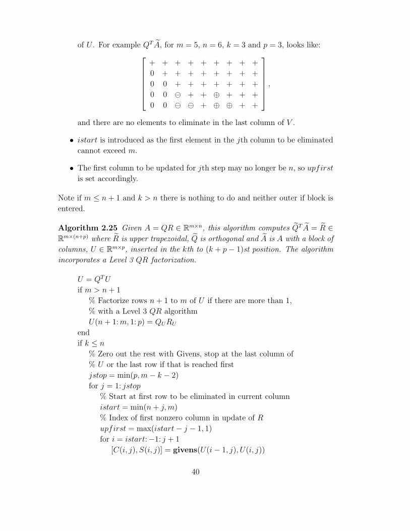
of U . For example QT A, for m = 5, n = 6, k = 3 and p = 3, looks like:
+ + + + + + + + +
0 + + + + + + + +
0 0 + + + + + + +
0 0 ⊖ + + ⊕ + + +
0 0 ⊖ ⊖ + ⊕ ⊕ + +
,
and there are no elements to eliminate in the last column of V .
• istart is introduced as the first element in the jth column to be eliminated
cannot exceed m.
• The first column to be updated for jth step may no longer be n, so upfirst
is set accordingly.
Note if m ≤ n + 1 and k > n there is nothing to do and neither outer if block is
entered.
Algorithm 2.25 Given A = QR ∈ Rm×n, this algorithm computes QT A = R ∈
Rm×(n+p) where R is upper trapezoidal, Q is orthogonal and A is A with a block of
columns, U ∈ Rm×p, inserted in the kth to (k + p − 1)st position. The algorithm
incorporates a Level 3 QR factorization.
U = QT U
if m > n + 1
% Factorize rows n + 1 to m of U if there are more than 1,
% with a Level 3 QR algorithm
U(n + 1: m, 1: p) = QURU
end
if k ≤ n
% Zero out the rest with Givens, stop at the last column of
% U or the last row if that is reached first
jstop = min(p, m − k − 2)
for j = 1: jstop
% Start at first row to be eliminated in current column
istart = min(n + j, m)
% Index of first nonzero column in update of R
upfirst = max(istart − j − 1, 1)
for i = istart:−1: j + 1
[C(i, j), S(i, j)] = givens(U(i − 1, j), U(i, j))
40
% Update U
U(i − 1, j) = C(i, j)U(i − 1, j) − S(i, j)U(i, j)
if j < p
% Update U
U(i − 1: i, j + 1: p) =[C(i, j) S(i, j)
−S(i, j) C(i, j)
]T
U(i − 1: i, j + 1: p)
end
% Update R
R(i − 1: i, upfirst: n) =[C(i, j) S(i, j)
−S(i, j) C(i, j)
]T
R(i − 1: i, upfirst: n)
% Update one more column next i step
upfirst = upfirst − 1
end
end
end
if k = 1
R = upper triangular part of [ U R ]
else if k = n + 1
R = upper triangular part of [ R U ]
else
R = upper triangular part of [ R(1: m, 1: k − 1) U R(1: m, k: n) ]
end
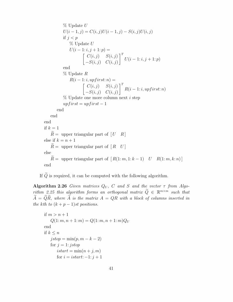
If Q is required, it can be computed with the following algorithm.
Algorithm 2.26 Given matrices QU , C and S and the vector τ from Algo-
rithm 2.25 this algorithm forms an orthogonal matrix Q ∈ Rm×m such that
A = QR, where A is the matrix A = QR with a block of columns inserted in
the kth to (k + p − 1)st positions.
if m > n + 1
Q(1: m, n + 1: m) = Q(1: m, n + 1: m)QU
end
if k ≤ n
jstop = min(p, m − k − 2)
for j = 1: jstop
istart = min(n + j, m)
for i = istart:−1: j + 1
41
Q(1: m, i − 1: i) = Q(1: m, i − 1: i)
[C(i, j) S(i, j)
−S(i, j) C(i, j)
]
end
end
end
Q = Q
See Appendix 6.5 for Fortran codes addcols.f and addcolsq.f for updating
R and Q respectively.
3 Error Analysis
It is well known that orthogonal transformations are stable. We have the following
columnwise results [10], where
γk =cku
1 − cku,
and u is the unit roundoff and c is a small integer constant.
Lemma 3.1 (Sequence of Givens Matrices) If
B = Gr . . . G1A = QT A ∈ Rn×n
where Gi is a Givens matrix, then the computed matrix B satisfies
QT A − B = ∆B, ‖∆bj‖2 ≤ γr‖aj‖2, j = 1: n. (3.1)
Lemma 3.2 (Sequence of Householder Matrices) If
B = Hr . . .H1A = QT A ∈ Rn×n
where Hi is a Householder matrix, then the computed matrix B satisfies
QT A − B = ∆B, ‖∆bj‖2 ≤ γnr‖aj‖2, j = 1: n. (3.2)
This result implies that Householder transformations are less accurate by a factor
of n, but this is not observed in practice. We then have
42

Theorem 3.1 (Householder QR Factorization) If
R = QT A
where Q is a product of Householder matrices, then the computed factor R satisfies
QT A − R = ∆R, ‖∆rj‖2 ≤ γmn‖aj‖2, j = 1: n.
We now give results for computing the factor R by our algorithms.
3.1 Deleting Rows
We have from Section 2.1.2
G(1, 2)T . . . G(m − 1, m)T R =
[vT
R
],
and from (3.1) we have for the computed quantitiesR and v
R = R + ∆R, ‖∆rj‖2 ≤ γmp
∥∥∥∥[
vT (j)
r(1: n, j)
]∥∥∥∥2
, j = 1: n.
Recall that the G(i, j) are chosen to introduce zeros in Q.
3.2 Adding Rows
We have from Section 2.3.2
Hn . . .H1
[R
U
]= R, U ∈ R
p×n,
and from (3.2) we have
R = R + ∆R, ‖∆rj‖2 ≤ γn(p+1)
∥∥∥∥[
rjj
U(: , j)
]∥∥∥∥2
, j = 1: n.
3.3 Deleting Columns
We have from Section 2.4.2
Hn−p . . .Hk [ R(: , 1: k − 1) R(: , k + p: n) ] = R,
43

and from (3.2) we have
R = R +
[0
∆R
], ∆R ∈ R
(m−k+1)×n
‖∆rj‖2 = 0, j = 1: k − 1,
≤ γ(n−k−p+1)(n−k+1)‖r(k: n, j)‖2, j = k: n − p.
3.4 Adding Columns
We have from Section 2.5.2
G(k + 2p − 2, k + 2p − 1) . . .
G(k + p − 1, k + p)
[I 0
0 QTV
][ R(: , 1: k − 1) V R(: , k: n) ] = R,
where V = QT U ∈ Rm×p and from (3.1) and (3.2) we have
R = R +
0
0
∆H
+
0
∆G
, ∆H ∈ R
(m−n)×n, ∆G ∈ R(m−k+1)×n
‖∆Hj‖2 = 0, k − 1 ≥ j ≥ k + p,
≤ γ(n−k)p‖V (n + 1: m, j)‖2, j = k: k + p − 1,
‖∆Gj‖2 = 0, j = 1: k − 1,
≤ γ(n−k)n
∥∥∥∥(QT V )(k: m, j) +
[0
∆rj
]∥∥∥∥2
, j = k: n + p.
Given these results we expect the normwise backward error
‖A − QR‖2
‖A‖2
,
when Q and R are computed with our algorithms to be close to that with Q and
R computed directly from A. We consider some examples in the next section.
4 Numerical Experiments
4.1 Speed Tests
In this section we test the speed of our double precision Fortran 77 codes, see
Appendix 6.5, against LAPACK’s DGEQRF, a Level 3 BLAS routine for computing
44

the QR factorization of a matrix. The input matrix, in this case A, is overwritten
with R, and Q is returned in factored form in the same way as our codes do.
The tests were performed on a 1400MHz AMD Athlon running Red Hat Linux
version 6.2 with kernel 2.2.22. The unit roundoff u ≈ 1.1e-16.
We tested our code with
m = {1000, 2000, 3000, 4000, 5000}
and n = 0.3m, and the number of columns added or deleted was p = 100. We
generated our test matrices by populating an array with random double precision
numbers generated with the LAPACK auxiliary routine DLARAN. A = QR was
computed with DGEQRF, and A was formed appropriately.
We timed our codes acting on QT A, the starting point for computing R, and in
the case of adding columns we included the computation of QT U in our timings,
which we formed with the BLAS routine DGEMM. We also timed DGEQRF acting
on only the part of QT A that needs to be updated, the nonzero part from row
and column k onwards. Here we can construct R with this computation and the
original R. Finally, we compute DGEQRF acting on A. We aim to show our codes
are faster than these alternatives. In all cases an average of three timings are
given.
To test our code DELCOLS we first chose k = 1, the position of the first
column deleted, where the maximum amount of work is required to update the
factorization. We have
A = A(1: m, p + 1: n), and QT A = R(1: m, p + 1: n)
and timed:
• DGEQRF on A.
• DGEQRF on (QT A)(k: n, k: n − p) which computes the nonzero entries of
R(k: m, p + 1: n).
• DELCOLS on QT A.
The results are given in Figure 1. Our code is clearly much faster than recom-
puting the factorization from scratch with DGEQRF, and for n = 5000 there is a
speedup of 20. Our code is also faster than using DGEQRF on (QT A)(k: n, k: n−p),
where there is a maximum speedup of over 3.
We then tested for k = n/2 where much less work is required to perform the
updating, we have
A = [ A(1: m, 1: k − 1) A(1: m, k + p: n) ] , and
QT A = [ R(1: m, 1: k − 1) R(1: m, k + p: n) ]
45

1000 2000 3000 4000 50000
5
10
15
20
25
30
35
40
45
Number of rows, m, of matrix
Tim
es (
secs
)
DGEQRF on ADGEQRF on (QT A)(k:n, k:n − p)DELCOLS on QT A
Figure 1: Comparison of speed for DELCOLS with k = 1 for different m.
and timed:
• DGEQRF on (QT A)(k: n, k: n − p) which computes the nonzero entries of
R(k: m, k: n − p).
• DELCOLS on QT A.
The results are given in Figure 2. The timings for DGEQFR on A would,
of course, be the same as for k = 1, giving a maximum speedup of over 100
in this case. We achieve a speedup of approximately 3 over using DGEQRF on
(QT A)(k: n, k: n − p).
We then considered the effect of varying p with DELCOLS for fixed m = 3000,
n = 1000 and k = 1. As we delete more columns from A there are less columns
to update, but more work is required for each one. We chose
p = {100, 200, 300, 400, 500, 600 700, 800}
and timed:
• DGEQRF on A
46

1000 2000 3000 4000 50000
0.1
0.2
0.3
0.4
0.5
0.6
0.7
0.8
0.9
Number of rows, m, of matrix
Tim
es (
secs
)
DGEQRF on (QT A)(k:n, k:n − p)DELCOLS on QT A
Figure 2: Comparison of speed for DELCOLS with k = n/2 for different m.
• DGEQRF on (QT A)(k: n, k: n − p) which computes the nonzero entries of
R(k: m, k: n − p).
• DELCOLS on QT A.
The results are given in Figure 3. The timings for DELCOLS are relatively level
and peak at p = 300, whereas the timings for the other codes obviously decrease
with p. The speedup of our code decreases with p, and from p = 300 there is
little difference between our code and DGEQRF on (QT A)(k: n, k: n − p).
To test ADDCOLS we generated random matrices A ∈ Rm×n and U ∈ R
m×p,
and again use
m = {1000, 2000, 3000, 4000, 5000}n = 0.3m, and p = 100. We first set k = 1 where maximum updating is required.
We have
A = [U A ] , and QT A = [QT U R ]
and timed:
• DGEQRF on A.
47

100 200 300 400 500 600 700 8000
2
4
6
8
10
12
Number of columns, p , deleted from matrix
Tim
es (
secs
)
DGEQRF on ADGEQRF on (QT A)(k:n, k:n − p)DELCOLS on QT A
Figure 3: Comparison of speed for DELCOLS for different p.
• ADDCOLS on QT A, including the computation of QT U with DGEMM.
The results are given in Figure 4. Here our code achieves a speedup of over 3
for m = 5000 over the complete factorization of A.
We then tested for k = n/2, where less work is required to do the updating.
We have
A = [A(1: m, 1: k − 1) U A(1: m, k: n) ] , and
QT A = [R(1: m, 1: k − 1) QT U R(1: m, k: n) ]
and timed:
• DGEQRF on A, as above.
• DGEQRF on (QT A)(k: m, k: n+p) which computes R(k: m, k: n+p), including
the computation of QT U for which we again use DGEMM.
• ADDCOLS on QT A, including the computation of QT U .
48

1000 2000 3000 4000 50000
10
20
30
40
50
60
Number of rows, m, of matrix
Tim
es (
secs
)
DGEQRF on AADDCOLS on QT A
Figure 4: Comparison of speed for ADDCOLS with k = 1 for different m.
The results are given in Figure 5. Here we have a maximum speedup of
over 4 with our code against DGEQRF on A. We achieve a maximum speedup of
approximately 2 against DGEQRF on (QT A)(k: m, k: n + p).
We do not vary p as this increases the work for both our code and DGEQRF on
(QT A)(k: m, k: n + p) roughly equally.
4.2 Backward Error Tests
The tests here were performed on a 2545MHz AMD Pentium running a hybrid
version of Red Hat Linux 8 and 9 with kernel 2.4.20.
Here we test our code for updating Q and R; DELCOLS and DELCOLSQ for
deleting columns and ADDCOLS and ADDCOLSQ for adding columns. We did this in
the following way:
• We form a random matrix
A(0) = [ A1 U A2 ] , ‖A1‖F , ‖A2‖F , ‖U‖F of order 100,
49

1000 2000 3000 4000 50000
10
20
30
40
50
60
Number of rows, m, of matrix
Tim
es (
secs
)
DGEQRF on ADGEQRF on (QT A)(k:m,k:n + p)DELCOLS on QT A
Figure 5: Comparison of speed for ADDCOLS with k = n/2 for different m.
where A1 ∈ Rm×(k−1), A2 ∈ R
m×(n−k−p+1), U ∈ Rm×p.
• We then form the QR factorization
A(0) = Q(0)R(0) = Q(0) [ R1 RU R2 ] ,
where R1 ∈ Rm×(k−1), R2 ∈ R
m×(n−k−p+1), RU ∈ Rm×p, using the LAPACK
routines DGEQRF and DORGQR.
• Next, for
A = [ A1 A2 ] ,
we form
Q(0)T
A = [ R1 R2 ] ,
and call DELCOLS and DELCOLSQ to update the QR factorization of A, form-
ing
A = QR = [ R1 R2 ] ,
where R1 ∈ Rm×(k−1), R2 ∈ R
m×(n−k−p+1).
50

• We now compute the QR factorization of A(0) by updating Q and R. We
call ADDCOLS on
[ R1 QT U R2 ]
to form R(1) and then call ADDCOLSQ to form Q(1), so we have, in exact
arithmetic
A(0) = Q(1)R(1).
We then repeat this rep times and measure the normwise backward error
‖A(0) − Q(rep)R(rep)‖2
‖A‖2
.
We use every combination of the following set of parameters:
m = 500
n = {400, 500, 600}p = {50, 100, 150}k = {1, 51, . . . , n − p + 1}.
We then repeated the entire process, but with
‖U‖F of order 1e+9.
The results are given in Table 1 and Table 2. The error increases with the number
of repeats which is expected. However, the value is not effected significantly by
the value of ‖U‖F .
The smallest value of the error in every case was approximately of order 10u.
The worse case was still only of order 2 ∗ rep ∗ u.
Table 1: Normwise backward error for ‖U‖F order 100.
rep 5 50 500
Smallest error over all tests 1.146e-15 1.212e-15 1.223e-15
Largest error over all tests 5.031e-15 2.399e-14 1.252e-13
51

Table 2: Normwise backward error for ‖U‖F order 1e+9.
rep 5 50 500
Smallest error over all tests 8.298e-16 9.309e-16 9.576e-16
Largest error over all tests 4.381e-15 2.055e-14 1.014e-13
5 Conclusions
The speed tests show that our updating algorithms are faster than computing
the QR factorization from scratch or using the factorization to update columns
k onward, the only columns needing updating.
Furthermore, the normwise backward error tests show that the errors are
within the bound for computing the Householder QR factorization of A. Thus,
within the parameters of our experiments, the increase of speed is not at the
detriment of accuracy.
We propose the double precision Fortran 77 codes delcols.f, delcolsq.f,
addcols.f and addcolsq.f, and their single precision and complex equivalents,
be included in LAPACK.
6 Software Available
Here we list some software that is available to update the QR factorization and
least squares problem. An ’x’ in a routine indicates more than one routine for
different precisions or for real or complex data.
6.1 LINPACK
LINPACK [7] has three routines that update the least squares problem and the
QR factorization.
• xCHUD updates the least squares problem when a row has been added in the
(m + 1)st position.
• xCHDD updates the least squares problem when a row has been deleted from
the mth position, an implementation of Saunder’s algorithm.
52

• xCHEX update the least squares problem when the rows of A have been
permuted.
In all cases the transformation matrices are represented by a vectors of sines
and cosines, and Q is not constructed.
6.2 MATLAB
MATLAB [11] supply three routines for updating the QR factorization only.
• qrdelete updates when one row or column is deleted from any position.
• qrinsert updates when one row or column is added to any position.
• qrupdate returns the factorization of A after a rank one change, that is
A = A + uvT , u ∈ Rm, v ∈ R
n.
In all cases both Q and R are returned.
6.3 The NAG Library
The Mark 20 NAG Library [12] contains routines for updating two cases.
• F06xPF performs the factorization
αuvT + R1 = QR1,
where
R =
[R1
0
], R =
[R1
0
], R1, R1 ∈ R
n×n,
and
Q = QQ.
Q is represented by vectors of sines and cosines.
• F06xQF performs the downdating problem
[R1
αvT
]= Q
[R1
0
],
where R, R and Q are as above.
53

6.4 Reichel and Gragg’s Algorithms
Reichel and Gragg [16] provide several Fortran 77 implementations of the algo-
rithms discussed in [6] for updating the QR factorization, returning both Q and
R. In all cases only m ≥ n is handled. The routines use BLAS like routines for
matrix and vector operations written for optimal performance on the test ma-
chine used in [16]. No error results are given for the Fortran routines, although
some results are given for the Algol implementations in [6].
• DDELR updates after one row is deleted; this algorithm varies from ours and
uses a Gram-Schmidt re-orthogonalization process.
• DINSR updates when one row is added, and is similar to our algorithm.
• DDELC updates when one column is deleted, and is similar to our algorithm.
• DINSC updates after one column is added; this algorithm varies from ours
and again uses a Gram-Schmidt re-orthogonalization process.
• DRNK1 updates after a rank 1 modification to A.
• DRRPM updates when A is A with some if its columns permuted.
6.5 What’s new in our algorithms
Our contribution is:
• We deal with adding/deleting block of p row/columns, and in two of the
four cases we exploit the Level 3 BLAS. Also, the Level 2 code for deleting
a block of rows is more efficient than calling the code for deleting one row
p times.
• In the case of updating the QR factorization we place no restrictions on m
and n.
• All our codes call existing BLAS and LAPACK routines.
54

In these Fortran files the dimension n refers to the number of columns in A,
and not A.
A delcols.f
SUBROUTINE DELCOLS( M, N, A, LDA, K, P, TAU, WORK, INFO )
*
* Craig Lucas, University of Manchester
* March, 2004
*
* .. Scalar Arguments ..
INTEGER INFO, K, LDA, M, N, P
* ..
* .. Array Arguments ..
DOUBLE PRECISION A( LDA, * ), TAU( * ), WORK( * )
* ..
*
* Purpose
* =======
*
* Given a real m by (n+p) matrix, B, and the QR factorization
* B = Q_B * R_B, DELCOLS computes the QR factorization
* C = Q * R where C is the matrix B with p columns deleted
* from the kth column onwards.
*
* The input to this routine is Q_B’ * C
*
* Arguments
* =========
*
* M (input) INTEGER
* The number of rows of the matrix C. M >= 0.
*
* N (input) INTEGER
* The number of columns of the matrix C. N >= 0.
*
* A (input/output) DOUBLE PRECISION array, dimension (LDA,N)
* On entry, the matrix Q_B’ * C. The elements in columns
* 1:K-1 are not referenced.
*
* On exit, the elements on and above the diagonal contain
* the n by n upper triangular part of the matrix R. The
* elements below the diagonal in columns k:n, together with
* TAU represent the orthogonal matrix Q as a product of
55

* elementary reflectors (see Further Details).
*
* LDA (input) INTEGER
* The leading dimension of the array A. LDA >= max(1,M).
*
* K (input) INTEGER
* The position of the first column deleted from B.
* 0 < K <= N+P.
*
* P (input) INTEGER
* The number of columns deleted from B. P > 0.
*
* TAU (output) DOUBLE PRECISION array, dimension(N-K+1)
* The scalar factors of the elementary reflectors
* (see Further Details).
*
* WORK DOUBLE PRECISION array, dimension (P+1)
* Work space.
*
* INFO (output) INTEGER
* = 0: successful exit
* < 0: if INFO = -I, the I-th argument had an illegal value.
*
* Further Details
* ===============
*
* The matrix Q is represented as a product of Q_B and elementary
* reflectors
*
* Q = Q_B * H(k) * H(k+1) *...* H(last), last = min( m-1, n ).
*
* Each H(j) has the form
*
* H(j) = I - tau*v*v’
*
* where tau is a real scalar, and v is a real vector with
* v(1:j-1) = 0, v(j) = 1, v(j+1:j+lenh-1), lenh = min( p+1, m-j+1 ),
* stored on exit in A(j+1:j+lenh-1,j) and v(j+lenh:m) = 0, tau is
* stored in TAU(j).
*
* The matrix Q can be formed with DELCOLSQ
*
* =====================================================================
*
* .. Parameters ..
56

DOUBLE PRECISION ONE
PARAMETER ( ONE = 1.0D+0 )
* ..
* .. Local Scalars ..
DOUBLE PRECISION AJJ
INTEGER J, LAST, LENH
* ..
* .. External Subroutines ..
EXTERNAL DLARF, DLARFG, XERBLA
* ..
* .. Intrinsic Functions ..
INTRINSIC MAX, MIN
* ..
*
* Test the input parameters.
*
INFO = 0
IF( M.LT.0 ) THEN
INFO = -1
ELSE IF( N.LT.0 ) THEN
INFO = -2
ELSE IF( LDA.LT.MAX( 1, M ) ) THEN
INFO = -4
ELSE IF( K.GT.N+P .OR. K.LE.0 ) THEN
INFO = -5
ELSE IF( P.LE.0 ) THEN
INFO = -6
END IF
IF( INFO.NE.0 ) THEN
CALL XERBLA( ’DELCOLS’, -INFO )
RETURN
END IF
*
LAST = MIN( M-1, N )
*
DO 10 J = K, LAST
*
* Generate elementary reflector H(J) to annihilate the nonzero
* entries below A(J,J)
*
LENH = MIN( P+1, M-J+1 )
CALL DLARFG( LENH, A( J, J ), A( J+1, J ), 1, TAU( J-K+1 ) )
*
IF( J.LT.N ) THEN
*
57
* Apply H(J) to trailing matrix from left
*
AJJ = A( J, J )
A( J, J ) = ONE
CALL DLARF( ’L’, LENH, N-J, A( J, J ), 1, TAU( J-K+1 ),
$ A( J, J+1 ), LDA, WORK )
A( J, J ) = AJJ
*
END IF
*
10 CONTINUE
*
RETURN
*
* End of DELCOLS
*
END
58

B delcolsq.f
SUBROUTINE DELCOLSQ( M, N, A, LDA, Q, LDQ, K, P, TAU, WORK, INFO )
*
* Craig Lucas, University of Manchester
* March, 2004
*
* .. Scalar Arguments ..
INTEGER INFO, K, LDA, LDQ, M, N, P
* ..
* .. Array Arguments ..
DOUBLE PRECISION A( LDA, * ), Q( LDQ, * ), TAU( * ), WORK( * )
* ..
*
* Purpose
* =======
*
* DELCOLSQ generates an m by m real matrix Q with orthogonal columns,
* which is defined as the product of Q_B and elementary reflectors
*
* Q = Q_B * H(k) * H(k+1) *...* H(last), last = min( m-1, n ) .
*
* where the H(j) are as returned by DELCOLSQ, such that C = Q * R and
* C is the matrix B = Q_B * R_B, with p columns deleted from the
* kth column onwards.
*
* Arguments
* =========
*
* M (input) INTEGER
* The number of rows of the matrix A. M >= 0.
*
* N (input) INTEGER
* The number of columns of the matrix A. N >= 0.
*
* A (input) DOUBLE PRECISION array, dimension (LDA,N)
* On entry, the elements below the diagonal in columns k:n
* must contain the vector which defines the elementary
* reflector H(J) as returned by DELCOLS.
*
* LDA (input) INTEGER
* The leading dimension of the array A. LDA >= max(1,M).
*
* Q (input/output) DOUBLE PRECISION array, dimension (LDA,N)
* On entry, the matrix Q_B.
59

* On exit, the matrix Q.
*
* LDQ (input) INTEGER
* The leading dimension of the array Q. LDQ >= M.
*
* K (input) INTEGER
* The position of the first column deleted from B.
* 0 < K <= N+P.
*
* P (input) INTEGER
* The number of columns deleted from B. P > 0.
*
* TAU (input) DOUBLE PRECISION array, dimension(N-K+1)
* TAU(J) must contain the scalar factor of the elementary
* reflector H(J), as returned by DELCOLS.
*
* WORK DOUBLE PRECISION array, dimension (P+1)
* Work space.
*
* INFO (output) INTEGER
* = 0: successful exit
* < 0: if INFO = -I, the I-th argument had an illegal value.
*
* =====================================================================
*
* .. Parameters ..
DOUBLE PRECISION ONE
PARAMETER ( ONE = 1.0D+0 )
* ..
* .. Local Scalars ..
DOUBLE PRECISION AJJ
INTEGER J, LAST, LENH
* ..
* .. External Subroutines ..
EXTERNAL DLARF, XERBLA
* ..
* .. Intrinsic Functions ..
INTRINSIC MAX, MIN
* ..
*
* Test the input parameters.
*
INFO = 0
IF( M.LT.0 ) THEN
INFO = -1
60

ELSE IF( N.LT.0 ) THEN
INFO = -2
ELSE IF( LDA.LT.MAX( 1, M ) ) THEN
INFO = -4
ELSE IF( K.GT.N+P .OR. K.LE.0 ) THEN
INFO = -5
ELSE IF( P.LE.0 ) THEN
INFO = -6
END IF
IF( INFO.NE.0 ) THEN
CALL XERBLA( ’DELCOLSQ’, -INFO )
RETURN
END IF
*
LAST = MIN( M-1, N )
*
DO 10 J = K, LAST
*
LENH = MIN( P+1, M-J+1 )
*
* Apply H(J) from right
*
AJJ = A( J, J )
A( J, J ) = ONE
*
CALL DLARF( ’R’, M, LENH, A( J, J ), 1, TAU( J-K+1 ),
$ Q( 1, J ), LDQ, WORK )
*
A( J, J ) = AJJ
*
10 CONTINUE
*
RETURN
*
* End of DELCOLSQ
*
END
61

C addcols.f
SUBROUTINE ADDCOLS( M, N, A, LDA, K, P, TAU, WORK, LWORK, INFO )
*
* Craig Lucas, University of Manchester
* March, 2004
*
* .. Scalar Arguments ..
INTEGER INFO, K, LDA, LWORK, M, N, P
* ..
* .. Array Arguments ..
DOUBLE PRECISION A( LDA, * ), TAU( * ), WORK( * )
* ..
*
* Purpose
* =======
*
* Given a real m by (n-p) matrix, B, and the QR factorization
* B = Q_B * R_B, ADDCOLS computes the QR factorization
* C = Q * R where C is the matrix B with p columns added
* in the kth column onwards.
*
* The input to this routine is Q_B’ * C
*
* Arguments
* =========
*
* M (input) INTEGER
* The number of rows of the matrix C. M >= 0.
*
* N (input) INTEGER
* The number of columns of the matrix C. N >= 0.
*
* A (input/output) DOUBLE PRECISION array, dimension (LDA,N)
* On entry, the matrix Q_B’ * C. The elements in columns
* 1:K-1 are not referenced.
*
* On exit, the elements on and above the diagonal contain
* the n by n upper triangular part of the matrix R. The
* elements below the diagonal in columns K:N, together with
* TAU represent the orthogonal matrix Q as a product of
* elementary reflectors and Givens rotations.
* (see Further Details).
*
* LDA (input) INTEGER
62

* The leading dimension of the array A. LDA >= max(1,M).
*
* K (input) INTEGER
* The position of the first column added to B.
* 0 < K <= N-P+1.
*
* P (input) INTEGER
* The number of columns added to B. P > 0.
*
* TAU (output) DOUBLE PRECISION array, dimension(P)
* The scalar factors of the elementary reflectors
* (see Further Details).
*
* WORK (workspace) DOUBLE PRECISION array, dimension ( LWORK )
* Work space.
*
* LWORK (input) INTEGER
* The dimension of the array WORK. LWORK >= P.
* For optimal performance LWORK >= P*NB, where NB is the
* optimal block size.
*
* INFO (output) INTEGER
* = 0: successful exit
* < 0: if INFO = -I, the I-th argument had an illegal value.
*
* Further Details
* ===============
*
* The matrix Q is represented as a product of Q_B, elementary
* reflectors and Givens rotations
*
* Q = Q_B * H(k) * H(k+1) *...* H(k+p-1) * G(k+p-1,k+p) *...
* *G(k,k+1) * G(k+p,k+p+1) *...* G(k+2p-2,k+2p-1)
*
* Each H(j) has the form
*
* H(j) = I - tau*v*v’
*
* where tau is a real scalar, and v is a real vector with
* v(1:n-p-j+1) = 0, v(j) = 1, and v(j+1:m) stored on exit in
* A(j+1:m,j), tau is stored in TAU(j).
*
* Each G(i,j) has the form
*
* i-1 i
63

* [ I ]
* [ c -s ] i-1
* G(i,j) = [ s c ] i
* [ I ]
*
* and zero A(i,j), where c and s are encoded in scalar and
* stored in A(i,j) and
*
* IF A(i,j) = 1, c = 0, s = 1
* ELSE IF | A(i,j) | < 1, s = A(i,j), c = sqrt(1-s**2)
* ELSE c = 1 / A(i,j), s = sqrt(1-c**2)
*
* The matrix Q can be formed with ADDCOLSQ
*
* =====================================================================
*
* .. Local Scalars ..
DOUBLE PRECISION C, S
INTEGER I, INC, ISTART, J, JSTOP, UPLEN
* ..
* .. External Subroutines ..
EXTERNAL DGEQRF, DLASR, DROT, DROTG, XERBLA
* ..
* .. Intrinsic Functions ..
INTRINSIC MAX, MIN
* ..
*
* Test the input parameters.
*
INFO = 0
IF( M.LT.0 ) THEN
INFO = -1
ELSE IF( N.LT.0 ) THEN
INFO = -2
ELSE IF( LDA.LT.MAX( 1, M ) ) THEN
INFO = -4
ELSE IF( K.GT.N-P+1 .OR. K.LE.0 ) THEN
INFO = -5
ELSE IF( P.LE.0 ) THEN
INFO = -6
END IF
IF( INFO.NE.0 ) THEN
CALL XERBLA( ’ADDCOLS’, -INFO )
RETURN
END IF
64

*
* Do a QR factorization on rows below N-P, if there is more than one
*
IF( M.GT.N-P+1 ) THEN
*
* Level 3 QR factorization
*
CALL DGEQRF( M-N+P, P, A( N-P+1, K ), LDA, TAU, WORK, LWORK,
$ INFO )
*
END IF
*
* If K not equal to number of columns in B and not <= M-1 then
* there is some elimination by Givens to do
*
IF( K+P-1.NE.N .AND. K.LE.M-1) THEN
*
* Zero out the rest with Givens
* Allow for M < N
*
JSTOP = MIN( P+K-1, M-1 )
DO 20 J = K, JSTOP
*
* Allow for M < N
*
ISTART = MIN( N-P+J-K+1, M )
UPLEN = N - K - P - ISTART + J + 1
*
INC = ISTART - J
*
DO 10 I = ISTART, J + 1, -1
*
* Recall DROTG updates A( I-1, J ) and
* stores C and S encoded as scalar in A( I, J )
*
CALL DROTG( A( I-1, J ), A( I, J ), C, S )
WORK( INC ) = C
WORK( N+INC ) = S
*
* Update nonzero rows of R
* Do the next two line this way round because
* A( I-1, N-UPLEN+1 ) gets updated
*
A( I, N-UPLEN ) = -S*A( I-1, N-UPLEN )
A( I-1, N-UPLEN ) = C*A( I-1, N-UPLEN )
65

*
CALL DROT( UPLEN, A( I-1, N-UPLEN+1 ), LDA,
$ A( I, N-UPLEN+1 ), LDA, C, S )
*
UPLEN = UPLEN + 1
INC = INC - 1
*
10 CONTINUE
*
* Update inserted columns in one go
* Max number of rotations is N-1, we’ve allowed N
*
IF( J.LT.P+K-1 ) THEN
*
CALL DLASR( ’L’, ’V’, ’B’, ISTART-J+1, K+P-1-J,
$ WORK( 1 ), WORK( N+1 ), A( J, J+1 ), LDA )
*
END IF
*
20 CONTINUE
*
END IF
RETURN
*
* End of ADDCOLS
*
END
66

D addcolsq.f
SUBROUTINE ADDCOLSQ( M, N, A, LDA, Q, LDQ, K, P, TAU, WORK, INFO)
*
* Craig Lucas, University of Manchester
* March, 2004
*
* .. Scalar Arguments ..
INTEGER INFO, K, LDA, LDQ, M, N, P
* ..
* .. Array Arguments ..
DOUBLE PRECISION A( LDA, * ), Q( LDQ, * ), TAU( * ), WORK( * )
* ..
*
* Purpose
* =======
*
* ADDCOLSQ generates an m by m real matrix Q with orthogonal columns,
* which is defined as the product of Q_B, elementary reflectors and
* Givens rotations
*
* Q = Q_B * H(k) * H(k+1) *...* H(k+p-1) * G(k+p-1,k+p) *...
* *G(k,k+1) * G(k+p,k+p+1) *...* G(k+2p-2,k+2p-1)
*
* where the H(j) and G(i,j) are as returned by ADDCOLS, such that
* C = Q * R and C is the matrix B = Q_B * R_B, with p columns added
* from the kth column onwards.
*
* Arguments
* =========
*
* M (input) INTEGER
* The number of rows of the matrix A. M >= 0.
*
* N (input) INTEGER
* The number of columns of the matrix A. N >= 0.
*
* A (input) DOUBLE PRECISION array, dimension (LDA,N)
* On entry, the elements below the diagonal in columns
* K:K+P-1 (if M > M-P+1) must contain the vector which defines
* the elementary reflector H(J). The elements above these
* vectors and below the diagonal store the scalars such that
* the Givens rotations can be constructed, as returned by
* ADDCOLS.
*
67

* LDA (input) INTEGER
* The leading dimension of the array A. LDA >= max(1,M).
*
* Q (input/output) DOUBLE PRECISION array, dimension (LDA,N)
* On entry, the matrix Q_B.
* On exit, the matrix Q.
*
* LDQ (input) INTEGER
* The leading dimension of the array Q. LDQ >= M.
*
* K (input) INTEGER
* The postion of first column added to B.
* 0 < K <= N-P+1.
*
* P (input) INTEGER
* The number columns added. P > 0.
*
* TAU (output) DOUBLE PRECISION array, dimension(N-K+1)
* The scalar factors of the elementary reflectors.
*
* WORK (workspace) DOUBLE PRECISION array, dimension (2*N)
* Work space.
*
* INFO (output) INTEGER
* = 0: successful exit
* < 0: if INFO = -I, the I-th argument had an illegal value
*
* =====================================================================
*
* .. Parameters ..
DOUBLE PRECISION ONE, ZERO
PARAMETER ( ONE = 1.0D+0, ZERO = 0.0D+0 )
* ..
* .. Local Scalars ..
DOUBLE PRECISION DTEMP
INTEGER COL, I, INC, ISTART, J, JSTOP
* ..
* .. External Subroutines ..
EXTERNAL DLARF, DLASR, XERBLA
* ..
* .. Intrinsic Functions ..
INTRINSIC ABS, MAX, MIN, SQRT
*
* Test the input parameters.
*
68

INFO = 0
IF( M.LT.0 ) THEN
INFO = -1
ELSE IF( N.LT.0 ) THEN
INFO = -2
ELSE IF( LDA.LT.MAX( 1, M ) ) THEN
INFO = -4
ELSE IF( K.GT.N-P+1 .OR. K.LE.0 ) THEN
INFO = -5
ELSE IF( P.LE.0 ) THEN
INFO = -6
END IF
IF( INFO.NE.0 ) THEN
CALL XERBLA( ’ADDCLQ’, -INFO )
RETURN
END IF
*
* We did a QR factorization on rows below N-P+1
*
IF( M.GT.N-P+1 ) THEN
*
COL = N - P + 1
DO 10 J = K, K + P - 1
*
DTEMP = A( COL, J )
A( COL, J ) = ONE
*
* If N+P > M-N we have only factored the first M-N columns.
*
IF( M-COL+1.LE.0 )
$ GO TO 10
CALL DLARF( ’R’, M, M-COL+1, A( COL, J ), 1, TAU( J-K+1 ),
$ Q( 1, COL ), LDQ, WORK )
*
A( COL, J ) = DTEMP
COL = COL + 1
*
10 CONTINUE
END IF
*
* If K not equal to number of columns in B then there was
* some elimination by Givens
*
IF( K+P-1.LT.N .AND. K.LE.M-1 ) THEN
*
69

* Allow for M < N, i.e DO P wide unless hit the bottom first
*
JSTOP = MIN( P+K-1, M-1 )
DO 30 J = K, JSTOP
*
ISTART = MIN( N-P+J-K+1, M )
INC = ISTART - J
*
* Compute vectors of C and S for rotations
*
DO 20 I = ISTART, J + 1, -1
*
IF( A( I, J ).EQ.ONE ) THEN
WORK( INC ) = ZERO
WORK( N+INC ) = ONE
ELSE IF( ABS( A( I, J ) ).LT.ONE ) THEN
WORK( N+INC ) = A( I, J )
WORK( INC ) = SQRT( ( 1-A( I, J )**2 ) )
ELSE
WORK( INC ) = ONE / A( I, J )
WORK( N+INC ) = SQRT( ( 1-WORK( INC )**2 ) )
END IF
INC = INC - 1
20 CONTINUE
*
* Apply rotations to the Jth column from the right
*
CALL DLASR( ’R’, ’V’, ’b’, M, ISTART-I+1, WORK( 1 ),
$ WORK( N+1 ), Q( 1, I ), LDQ )
*
30 CONTINUE
*
END IF
RETURN
*
* End of ADDCOLS
*
END
70

References
[1] A. Bjorck. Numerical Methods for Least Squares Problems. SIAM, Philadel-phia, PA, USA, 1996.
[2] A. Bjorck, L. Elden, and H. Park. Accurate downdating of least squaressolutions. SIAM J. Matrix Anal. Appl., 15:549–568, 1994.
[3] A. W. Bojanczyk, R. P. Brent, P. Van Dooren, and F. R. De Hoog. A noteon downdating the Cholesky factorization. SIAM J. Sci. Stat. Comput., 8(3):210–221, 1987.
[4] Adam Bojanczyk, Nicholas J. Higham, and Harikrishna Patel. Solving theindefinite least squares problem by hyperbolic QR factorization. SIAM J.
Matrix Anal. Appl., 24(4):914–931, 2003.
[5] J. M. Chambers. Regression updating. Journal of the American Statistical
Association, 66(336):744–748, 1971.
[6] J. W. Daniel, W. B. Gragg, L. Kaufman, and G. W. Stewart. Reorthogonal-ization and stable algorithms for updating the Gram–Schmidt QR factoriza-tion. Mathematics of Computation, 30(136):772–795, 1976.
[7] J. J. Dongarra, C. B. Moler, J. R. Bunch, and G. W. Stewart. LINPACK
Users’ Guide. Society for Industrial and Applied Mathematics, Philadelphia,PA, USA, 1979.
[8] L. Elden and H. Park. Block downdating of least squares solutions. SIAM
J. Matrix Anal. Appl., 15:1018–1034, 1994.
[9] G. H. Golub and C. F. Van Loan. Matrix Computations. Third edition, TheJohns Hopkins University Press, Baltimore, MD, USA, 1996.
[10] Nicholas J. Higham. Accuracy and Stability of Numerical Algorithms. Secondedition, Society for Industrial and Applied Mathematics, Philadelphia, PA,USA, 2002.
[11] MATLAB, version 6.5. The Mathworks Inc, Natick, MA, USA.
[12] NAG Fortran Library Manual, Mark 20. Numerical Algorithms Group, Ox-ford, UK.
[13] S. J. Olszanskyj, J. M. Lebak, and A. W. Bojanczyk. Rank-k modificatonmethods for recursive least squares problems. Numerical Algorithms, 7:325–354, 1994.
[14] B. N. Parlett. Analysis of algorithms for reflections in bisectors. SIAM
Review, 13:197–208, 1971.
71

[15] C. M. Rader and A. O. Steinhardt. Hyperbolic Householder transforms.SIAM J. Matrix Anal. Appl., 9(2):269–290, 1988.
[16] L. Reichel and W. B. Gragg. Algorithm 686: FORTRAN subroutines forupdating the QR decomposition. ACM Trans. Math. Soft., 16:369–377, 1990.
[17] M. A. Saunders. Large-scale linear programming using the cholesky factor-ization. Technical Report CS252, Computer Science Department, StanfordUniversity, CA, 1972.
[18] Robert Schreiber and Charles van Loan. A storage-efficient wy representa-tion for products of householder transformations. SIAM J. Sci. Stat. Com-
put., 10(1):53–57, 1989.
[19] G. W. Stewart. The effects of rounding error on an algorithm for downdatinga Cholesky factorization. Journal of the Institute of Mathematics and its
Applications, 23(2):203–213, 1979.
[20] G. W. Stewart. On the stability of sequential updates and downdates. IEEE
Trans. Signal Processing, 43(11):2642–2648, 1995.
72