generalized qr factorization and its applications* e

Generalized QR Factorization and Its Applications*

E . Anderson

Cray Research Inc.

655F Lone Oak Drive

Eagan, Minnesota 55121

Z. Bai

Department of Mathematics

University of Kentucky

Lexington, Kentucky 40506

and

J. Dongarra

Department of Computer Science

The University of Tennessee

Knoxvilk, Tennessee 37996

and

Mathematical Sciences Section

Oak Ridge National Laboratory

Oak Ridge, Tennessee 37831

Submitted by F. Uhlig

ABSTRACT

The purpose of this paper is to reintroduce the generalized QR factorization with or

without pivoting of two matrices A and B having the same number of rows. When B is

square and nonsingular, the factorization implicitly gives the orthogonal factorization of

B-‘A. Continuing the work of Paige and Hammarling, we discuss the different forms of

the factorization from the point of view of general-purpose software development.

*This work was supported in part by NSF grant ASC-8715728, and in part by the

Applied Mathematical Sciences subprogram of the Office of Energy Research, U.S. Depart-

ment of Energy, under Contract DE-AC05-840R21400.

LZNEAR ALGEBRA AND ITS APPLICATIONS 162-164:243-271 (1992) 243

0 Elsevier Science Publishing Co., Inc., 1992

655 Avenue of the Americas, New York, NY 10010 0024.3795/92/$5.00

244 E. ANDERSON, Z. BAI, AND J. DONGARRA

In addition, we demonstrate the applications of the GQR factorization in solving the linear equality-constrained least-squares problem and the generalized linear regression problem, and in estimating the conditioning of these problems.

1. INTRODUCTION

The QR factorization of an n x m matrix A assumes the form

A = QR

where Q is an n x n orthogonal matrix, and R = QrA is zero below its diagonal. If n 2 m, then QTA can be written in the form

Q=A = “d’ [ I

where R,, is an n x n upper triangular matrix. If n < m, then the QR factorization of A assumes the form

QTA = [RI, RI,]

where RI1 is an n x n upper triangular matrix. However, in practical applications, it is more convenient to represent the factorization in this case as

which is known as the RQ factorization. Closely related to the QR and RQ

factorizations are the QL and LQ factorizations, which are orthogonal-lower- triangular and lower-triangular-orthogonal factorizations, respectively. It is well known that the orthogonal factors of A provide information about its

column and row spaces [lo]. A column pivoting option in the QR factorization allows the user to detect

dependencies among the columns of a matrix A. If A has rank k, then there are an orthogonal matrix Q and a permutation matrix P such that

Q=AP= [ ‘;’ ‘;‘I:_,

k m-k

QR FACTORIZATION 245

where R,, is k x k, upper triangular, and nonsingular [lo]. Householder transformation matrices or Givens rotation matrices provide numerically stable numerical methods to compute these factorizations with or without pivoting [lo]. The software for computing the QR factorization on sequential machines is available from the public linear-algebra library LINPACK [8]. Redesigned codes in block algorithm fashion that are better suited for today’s high-performance architectures will be available in LAPACK [l].

The terminology generalized QR factorization (GQR factorization), as used by Hammarling [12] and Paige [20], refers to the orthogonal transformations that simultaneously transform an n x m matrix A and an n x p matrix B to triangular form. This decomposition corresponds to the QR factorization of B-‘A when B is square and nonsingular. For example, if n 2 m, n < p, then the GQR factorization of A and I3 assumes the form

Q=A = [ ;], Q=BV= [o s],

where Q is an n x n orthogonal matrix or a nonsingular well-conditioned matrix, V is a p x p orthogonal matrix, R is m x m and upper triangular, and S is p x p and upper triangular. If B is square and nonsingular, then the QR factorization of B-‘A is given by

V=(B-‘A) = [ ;] = S-‘[ ;I,

i.e., the upper triangular part T of the QR factorization of B- ‘A can be determined by solving the triangular matrix equation

S,,T = R,

where S,, is the m x m top left comer block of the matrix S. This implicit determination of the QR factorization of B- ‘A avoids the possible numerical difficulties in forming B-’ or B-‘A.

Just as the QR factorization has proved to be a powerful tool in solving least-squares and related linear regression problems, so too can the GQR factorization be used to solve both the linear equality-constrained least-squares problem

min (1 AX - bll, Br=d

246

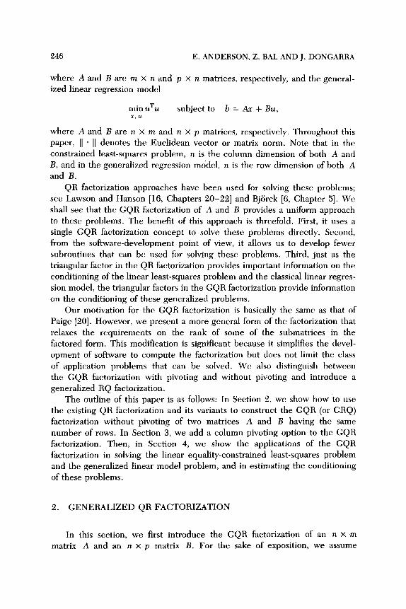
where A and B are m x n and ized linear regression model

min uTu x, U

where A and B are n x m and

E. ANDERSON, Z. BAI, AND J. DONGARRA

p x n matrices, respectively, and the general-

subject to b = Ax + Bu,

n x p matrices, respectively. Throughout this paper, ]] * 11 denotes the Euclidean vector or matrix norm. Note that in the constrained least-squares problem, n is the column dimension of both A and B, and in the generalized regression model, n is the row dimension of both A and B.

QR factorization approaches have been used for solving these problems; see Lawson and Hanson [16, Chapters 20-221 and Bjiirck [6, Chapter 51. We shall see that the GQR factorization of A and B provides a uniform approach to these problems. The benefit of this approach is threefold. First, it uses a single GQR factorization concept to solve these problems directly. Second, from the software-development point of view, it allows us to develop fewer subroutines that can be used for solving these problems. Third, just as the triangular factor in the QR factorization provides important information on the conditioning of the linear least-squares problem and the classical linear regression model, the triangular factors in the GQR factorization provide information on the conditioning of these generalized problems.

Our motivation for the GQR factorization is basically the same as that of Paige [20]. However, we present a more general form of the factorization that relaxes the requirements on the rank of some of the submatrices in the factored form. This modification is significant because it simplifies the development of software to compute the factorization but does not limit the class of application problems that can be solved. We also distinguish between the GQR factorization with pivoting and without pivoting and introduce a generalized RQ factorization.

The outline of this paper is as follows: In Section 2, we show how to use the existing QR factorization and its variants to construct the GQR (or GRQ) factorization without pivoting of two matrices A and B having the same number of rows. In Section 3, we add a column pivoting option to the GQR factorization. Then, in Section 4, we show the applications of the GQR factorization in solving the linear equality-constrained least-squares problem and the generalized linear model problem, and in estimating the conditioning of these problems.

2. GENERALIZED QR FACTORIZATION

In this section, we first introduce the GQR factorization of an n X m matrix A and an n x p matrix B. For the sake of exposition, we assume


n 2 m, the most frequently occurring case. Then, for the case n < m, we introduce the GRQ factorization of A and B.

GQR factorization. Let A be an n x m matrix, B an n X p matrix, and assume that n 2 m. Then there are orthogonal matrices Q (n x m) and V (pxp) suchthat

Q’A = R, Q=BV = S, (1)

where

R= R1l ;_,, [ I 0

with R,, (m x m) upper triangular, and

s= [o Sll], if n<p p-n n

where the n x n matrix S,, is upper triangular, or

S 11

[ I “-P

s = s,, P if n>p,

P

where the p x p matrix S,, is upper triangular.

Proof. The proof is easy and constructive. By the QR factorization of A we have

QTA= “d’ ;_,. [ 1

m

Let QT premultiply B; then the desired factorizations follow upon the RQ factorization of QTB. If n Q p,

(QTB)v= 1’ ‘llln; p-r3 n


otherwise, the RQ factorization of QTB has the form

To illustrate these decompositions we give examples for each case:

EXAMPLE. Suppose A and B are each 4 x 3 matrices given by

Then in the GQR factorization of A and B, the computed orthogonal matrices’ Q and V are

-0.2085 -0.8792 0.1562 -0.3989

Q= 0.6255 -0.4147 0.1465 0.6444 -0.4170 -0.2322 -0.7665 0.4296 ' -0.6255 0.0332 0.6054 0.4910

1 0.5275 -0.3229

-0.2982 -0.9365 I > 0.7955 -0.1369

and R and S are

-4.7958 1.4596 -0.8341

R= 0 -2.6210 0 0 2.5926 ' 0 0 -2.7537 1 0

-4.2220 3.1170 0.8223

S= -4.0063 1.8176 0 -2.0602 -1.7712 1 -0.4223 ' 0 0 3.5872

‘In all of these examples, the computed results are presented to four decimal digits,

although the computations were carried out in double precision. If the computed variables

are on the order of machine precision, (i.e., 2.2204~016), we round to zero.

QR FACTORIZATION

To illustrate the case n < p, let B be given by

12 3 4 5

B= [ -3 2 -2 1 2 1 ; 2 3 4 -2 -1 13-2 2 1

then in the GQR factorization of A and B, the orthogonal matrix V is

I

0.3375 -0.0791 -0.2689 -0.6363 0.6345 0.8926 0.2044 -0.1635 0.2771 -0.2407

v= -0.0534 -0.5118 -0.5794 -0.2833 -0.5651 0.1585 0.1280 0.6087 -0.6280 -0.4401

-0.2478 0.8208 -0.4414 -0.2091 -0.1626

and the matrix S is

0 7.0240 2.1937 0.1571

-3.4311 2.8692 - 1.8585 0.1389 1 0 0 -5.9566 1.0776 ' 0 0 0 3.9630

249

Occasionally, one wishes to compute the QR factorization of B- ‘A, for example, to solve the weighted least-squares problem

rnjnI[ B-‘( Ax - b)II.

To avoid forming B- ’ and B-‘A, we note that the GQR factorization (1) of A and B implicitly gives the QR factorization of B-lA:

VT(B-lA) = [;I = S-f';'],

i.e., the upper triangular part T of the QR factorization of B-‘A can be determined by solving the triangular system

SllT = Rll

for T, where S,, is the m x m top left corner block of the matrix S. Hence, the possible numerical difficulties in using, explicitly or implicitly, the QR factorization of B-‘A are confined to the conditioning of S,,.


Moreover, if we partition V = [V, V’s], where V, has m columns, then

B-IA = Vr( S,‘R,,).

This shows that if A is of rank m, the columns of V, form an orthonormal basis for the space spanned by the columns of B- ‘A. The matrix VrVr’ is the orthogonal projection onto W (B-IA), where 9 (*) denotes the range or column space.

Another straightforward application of the GQR factorization is to find a maximal set of BBT-orthonormal vectors orthogonal to g(A). That is, we want to find a matrix Z such that

ZTA = 0, ZTBBTZ = 1.

Let us rewrite the decomposition (1) as

where Q is partitioned conformally with R,

and S,,, S,, are upper triangular. Then the desired matrix Z is given by

Z = Q2SAT.

When A is an n x m matrix with n < m, although it still can be presented in forms similar to that of the GQR factorization of A and B, it is sometimes more useful in applications to represent the factorization as the following:

GRQ factorization. Let A be an n x m matrix, B an n x p matrix, and

assume that n < m. Then there are orthogonal matrices Q (n x n) and U

(m x m) such that

QTAU = R, QTB = S, (2)

R = Lo Rllln, m-n n


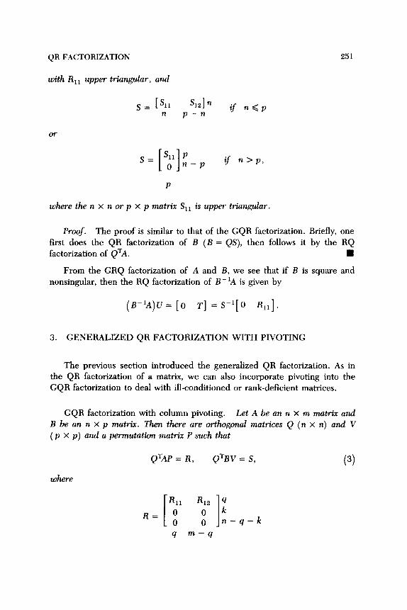
with R,, upper triangular, and

S= Pll s12ln n p-n

or

s= Sll P

[ 1 0 n-p

if nQp

if n>p,

P

where the n x n or p x p matrix S,, is upper triangular.

Proof. The proof is similar to that of the GQR factorization. Briefly, one first does the QR factorization of B (B = QS), then follows it by the RQ factorization of QTA. n

From the GRQ factorization of A and B, we see that if B is square and nonsingular, then the RQ factorization of B- ‘A is given by

(B-~A)u= [O T] = s-l[o R,,].

3. GENERALIZED QR FACTORIZATION WITH PIVOTING

The previous section introduced the generalized QR factorization. As in the QR factorization of a matrix, we can also incorporate pivoting into the GQR factorization to deal with ill-conditioned or rank-deficient matrices.

GQR factorization with column pivoting. Let A be an n x m matrix and

B be an n x p matrix. Then there are orthogonal matrices Q (n x n) and V

( p x p) and a permutation matrix P such that

where

QTAP = R, QTBV = S, (3)

R 11 42

R= ; ; [ 1 ;z

n-q-k

q m-q


the q x q matrix R,, is upper triangular and nonsingular, and either

p-n q n-q,

where the q x q matrix S,, is upper triangular and S,,, if it exists, is a

full-row-rank upper trapezoidal matrix, or

p-n+q n-q

if n>p

where S, 1, if it exists, is trapezoidal with zeros in the strictly lower le$ triangle,

and the k x (n - q) matrix S,, is full-row-rank upper trapezoidal. lf p < n - q.

then the first block column of S is not present.

Proof. The proof is also constructive. By the QR factorization with

pivoting of A, we have

QTAp= [“d’ ;‘I::-q. 9 m-q

where q = rank(A). If n Q p, let

(Q;B)V, = [i “:: 2$- 9

p-n 4 n-q

be the RQ factorization of QTB. Then by the QR factorization with pivoting on

the submatrix sz2, we have

n-q


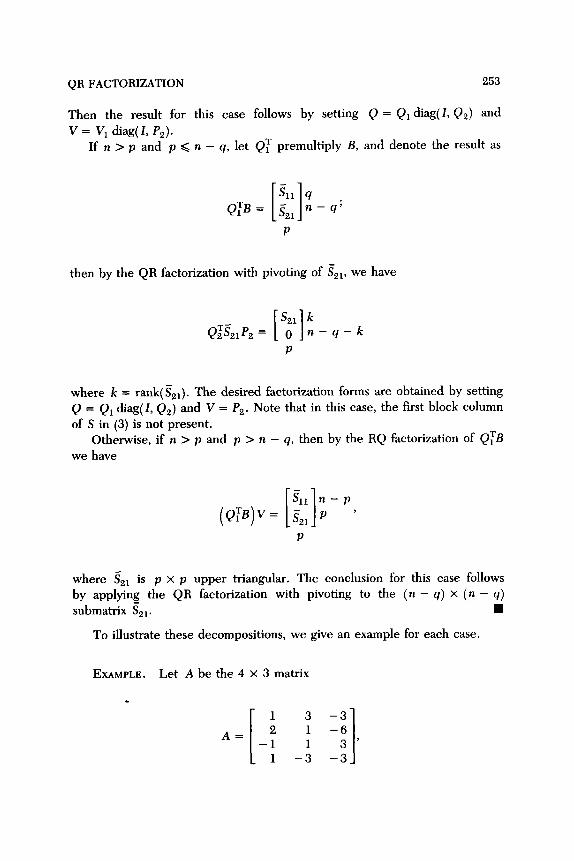
Then the result for this case follows by setting Q = Q1 diag( I,Qz) and

V = V, diag( 1, Pa). If n > p and p ,< n - Q, let QT premultiply B, and denote the result as

Sll q

QTB= i& n-q’ [- 1

P

then by the QR factorization with pivoting of ssr, we have

P

where k = rank($r). The desired factorization forms are obtained by setting

Q = Qr diag( I, Q2) and V = Pg. Note that in this case, the first block column

of S in (3) is not present. Otherwise, if n > p and p > n - q. then by the RQ factorization of QFB

we have

(Q:B)v= [l$ji-'.

P

where s2r is p x p upper triangular. The conclusion for this case follows

by applying the QR factorization with pivoting to the (n - q) x (n - q) submatrix $,. n

To illustrate these decompositions, we give an example for each case.

EXAMPLE. Let A be the 4 X 3 matrix

1 3 -3

A= [ _; : 1 -3 -3”, 1 -3

254 E.ANDERSON,Z.BAI,ANDJ.DONGARRA

where rank(A) = 2. To illustrate the case n < p, let B be the 4 x 5 matrix

1111 1

B= -1 3 2 3

2234 5' 1111 -2 1 1

Then in the GQR decomposition with column pivoting of A and B, we have

-0.3780 0.6412 Q= - 0.7559 0.1603

0.3780 0.2565 - 0.3780 - 0.7053

I

0.0930 -0.7658 - 0.5906 0.0188

v= 0.7674 0.2360 -0.0419 - 0.3350 - 0.2279 0.4953

P = [ e3 e2 e,],

0.1290 -0.3616 -0.8785 -0.2844

0.6553

- 0.5217 1 0.1400 ’ 0.5281

-0.2663 0.1663 -0.5535 -0.6319 -0.5007 0.0283 -0.3643 -0.4453 -0.1562 0.6002 -0.7234 -0.0497 0.1918 -0.0009 -0.8161

where ej is the ith column of an identity matrix 1. The matrices R and S are

R= [

7.9373 - 0.3780 - 2.6458

0 4.4561 0 0 0 0 0 0 0

1 '

[ 0.0000 0.9277 1.2449 2.8575 - 2.3896 - -

s= 0 0 0 1.9188 1.0978 0 0 0 6.2502 4.6798 ’ 0 0 0 0 -3.5863

1 To illustrate the case rr > p and p < n - 9. let B be the 4 x 2 matrix

2 3

B= [ 2 3 1 2 3' 21

Then the GQR decomposition with column pivoting of A and B gives

[

-0.3780 0.6412 0.1290 0.6553

Q= -0.7559 0.1603 -0.3616 -0.5217 0.3780 0.2565 -0.8785 0.1400 ' -0.3780 -0.7053 -0.2844 0.5281

I

v= [e2 cl],


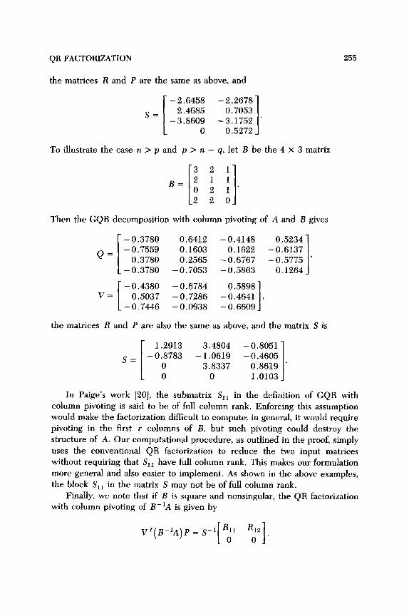
the matrices R and P are the same as above, and

To illustrate the case n > p and p > n - 9. let B be the 4 x 3 matrix

3 2 1

R= [ 2 1

0 2 2 2 1 1 1’

0

Then the GQR decomposition with column pivoting of A and B gives

[

- 0.3780 0.6412 - 0.4148 0.5234

Q= -0.7559 0.1603 0.1622 - 0.6137

0.3780 0.2565 -0.6767 -0.5775 ’ - 0.3780 -0.7053 -0.5863 0.1264 1 [ - 0.4380 - 0.6784 0.5898

v= 0.5037 -0.7286 -0.4641 , -0.7446 - 0.0938 -0.6609 1

the matrices R and P are also the same as above, and the matrix S is

[

1.2913 3.4804 - 0.8051

s= -0.8783 - 1.0619 - 0.4605

0 3.8337 0.8619 . 0 0 1.0103 1

In Paige’s work [20], the submatrix S,, in the definition of GQR with

column pivoting is said to be of full column rank. Enforcing this assumption

would make the factorization difficult to compute; in general, it would require

pivoting in the first r columns of B, but such pivoting could destroy the

structure of A. Our computational procedure, as outlined in the proof, simply

uses the conventional QR factorization to reduce the two input matrices

without requiring that S,, have full column rank. This makes our formulation

more general and also easier to implement. As shown in the above examples,

the block S,, in the matrix S may not be of full column rank.

Finally, we note that if B is square and nonsingular, the QR factorization

with column pivoting of B- ‘A is given by

V’( B-‘A) P = S- t “d’ Rd.


4. APPLICATIONS

In this section, we shall show that the GQR factorization not only provides a simpler and more efficient way to solve the linear equality-constrained least-squares problem and the generalized linear regression problem, but also provides an efficient way to assess the conditioning of these problems. Hence the GQR factorization for solving these generalized problems is just as powerful as the QR factorization is for solving least-squares and linear regression problems. In the next section, we shall briefly mention some other applications of the GQR factorization.

4.1. Linear Equality-Constrained Least Squares

The linear equality-constrained least-squares (LSE) problem arises in constrained surface fitting, constrained optimization, geodetic least-squares adjustment, signal processing, and other applications. The problem is stated as follows: find an n-vector r that solves

where A is an m x n matrix, m > n, B is a p x n matrix, p < n, b is an n-vector, and d is a p-vector. Clearly, the LSE problem has a solution if and only if the equation Bx = d is consistent. For simplicity, we shall assume that

rank(B) = p,

i.e., B has linearly independent rows, so that Bx = d is consistent for any right-hand side d. Moreover, we assume that the null spaces Jv( A) and “Y(B) of A and B intersect only trivially:

J(A) r3 J(B) = (0).

Then the LSE problem has a unique solution, which we denote by xe. We note that (6) is equivalent to the rank condition

rank

Several methods for solving the LSE problem are discussed in the books by Lawson and Hanson [16, Chapters 20-221 and Bjiirck [6, Chapter 51. For a


discussion of the large sparse matrix case, see Bjiirck [6], Van Loan [23], Barlow et al. [3], and Barlow [4]. The null-space approach via a two-step QR decomposition is one of the most general methods for dense matrices. Now this approach can be presented more easily in terms of the GQR factorization of A and B.

By the GQR factorization of BT and AT, we know that there are orthogonal matrices Q and U such that

0 Rll RlZ p s P

Q=A=U=R= 0 0 I

R,, n-P Q=B= = S = [ 1 ;’ n-p,

m-n p n-p P

and from the assumptions (4) and (7), we know S,, and R,, are upper triangular and nonsingular. If we partition

Q=[Q, Qz], u= [ul u, u,],

where Qi has p columns, Vi has m - n columns, and Us has p columns, and set

y = QTX = ‘I p

[ 1 ~2 n-p’

where yi = QTx, i = 1,2, and ci = UiTb, i = 1,2,3, then the LSE problem is

transformed to

subject to

[ST1 01[;;] =d-

Hence we can compute yi from the equality constraint by solving the triangular system

ST1 y, = d.


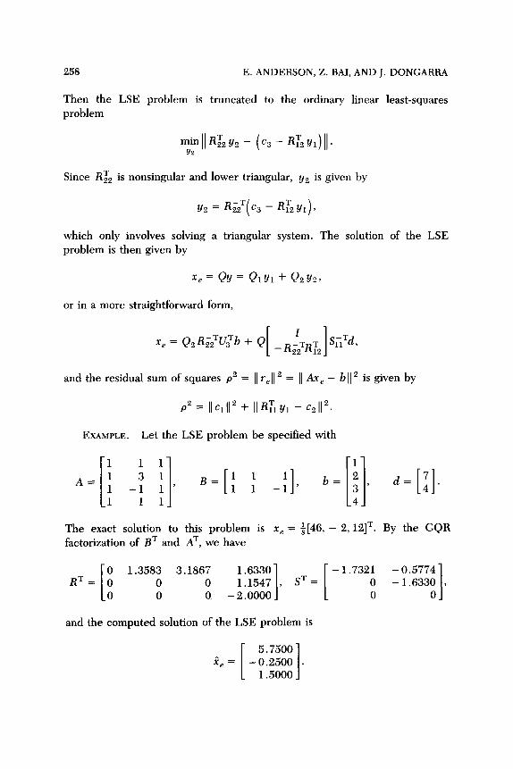
Then the LSE problem is truncated to the ordinary linear least-squares problem

Since Rz2 is nonsingular and lower triangular, yZ is given by

which only involves solving a triangular system. The solution of the LSE problem is then given by

or in a more straightforward form,

xt? = QdGQ-,Tb + Q _& [ 1 SLTd,

22 12

and the residual sum of squares p2 = 11 r, 11 2 = )I Ax, - b II 2 is given by

p2 = II ~1 II 2 + II R:, ~1 - ~2 II 2.

EXAMPLE. Let the LSE problem be specified with

1

A=; [

1 1

_; ;, 1 B= [; ; _:I>

1 1 1

b=[;]. d= [I].

The exact solution to this problem is X, = $[46, - 2, 121T. By the GQR factorization of BT and AT, we have

1.3583 3.1867 1.6330 - 1.7321 - 0.5774 0 0 1.1547 1 , ST= [ 0 -1.6330

I ,

0 0. - 2.0000 0 0

and the computed solution of the LSE problem is

5.7500 f, =

[ 1 -0.2500 . 1.5000


The relative error of the computed solution is

II?? - %I1 II XeII

= 4.2892 x 10-16,

and the norm of the residual ]I Ai, - b]] = 9.2466.

The Sensitivity of the LSE Problem. The condition numbers of A and B

were introduced by Elden [9] to assess the perturbed behavior of the LSE problem. Specifically, let E be an error matrix of A, F be an error matrix of B, and e and f be errors of b and d, respectively. We assume that B + F also has full row rank and “Y( A + E) fl Jv( B + F) = {0}, i.e., the perturbed LSE problem also has a unique solution. Let ge be the solution of the same

problem with A, B, b, and d replaced by A + E, B + F, b + e, and d + f,

respectively. Elden introduced the condition numbers

%I( A) = II All li( AG)+ll> “A(B) = l\Bll IlBf,ll

to measure the sensitivity of the LSE problem, where

G = I - B+B, Bl = [I - ( AG)+A] B+,

and At denotes the Moore-Penrose pseudoinverse of a matrix A.

Under mild conditions, Elden’s asymptotic perturbation bound, modified slightly here, can be presented as follows:

LSE-Problem Perturbation Bound.

II x, - Fell II xt? II

<x,(a)(;+..j +K,(B)(;+%)

+ K it lA) (

II E II II FII m + ‘dB)m pe+ ‘k”b

) where

II f4l ve = II All II xell ’

Ilf II -Y’ = II Bll II xell ’

II rt? II ” = II All II xell ’

r, = Ax, - b,

and Ok denotes the higher-order term in the perturbation matrices E, F, etc.

260 E. ANDERSON, Z. BAI. _4ND J. DONGARRA

The interpretation of this result is that the sensitivity of Xe is measured by K s( A) and K *(B) if the residual re is zero or relatively small, and otherwise by

‘6(A)]%@) + I]. We note that if the matrix B is zero (hence F = 0), then the LSE problem

is just the ordinary linear least-squares problem. The perturbation bound for the LSE problem is then reduced to

II-%?--eIl ll E II I- II ell II Tell ’ K(A) II All + II All II xell

lIEI Il~ell + K’(A) 11 A]\ )I AlI 11 x,JI + Ok”)

where K~(A) = K(A) = II AlI (1 A+ll. Th is is just the perturbation bound of the linear least-squares problem obtained by Golub and Wilkinson [lo].

Estimation of the Condition Numbers. The condition numbers K B( A) and K~( B) of the LSE problem involves Bt, I&, (AC)+. etc., and computing these matrices can be expensive. Fortunately, it is possible to compute inexpensive estimates of K~( A) and K~(B) without forming Bt, BtB, or ( AG)+. This can be done using a method of Hager [ll] and Higham [14] that computes a lower bound for ]I B ]I oD, where B is a matrix, given a means for evaluating matrix- vector products Bu and BTu. Typically, four or five products are required, and the lower bound is almost always within a factor 3 of )I I?]],. To estimate K~( A) and K~( B), we need to estimate vector norms )I Kz ]I m, where K = ( AG)+ or K = Sd, and z > 0 is a vector that is readily computed. Given the GQR factorization of A and B, after tedious computations, we have

(AG)+Z = 92 R~;u:z,

where we do not need to form RizT or S& T, but rather solve the triangular system and do matrix-vector operations.

Roughly speaking, the conditioning of the LSE problem only depends on the conditioning of the matrices R,, and S,,. In the last example, although the

matrix R is ill conditioned (actually, it is singular), we have

- 5.7735 1 -1.6330 ’ so it turns out to be a well-conditioned problem.


4.2. Generalized Linear Regression Model

The generalized linear regression model (GLM) problem can be written as

b = Ax + w, (8)

where w is a random error with mean 0 and a symmetric nonnegative definite variance-covariance matrix u2 W. The problem is that of estimating the unknown parameters x on the basis of the observation b. If W has rank p,

then W has a factorization

W = BBT.

where the n x p matrix B has linearly independent columns (for example, the Cholesky factorization of W could be carried out to get B). In some practical problems, the matrix B might be available directly. For numerical computa- tion reasons it is preferable to use B rather than W, since W could be ill conditioned, but the condition of B may be much better. Thus we replace (8)

by

b = Ax + Bu, (9)

where A is an n x m matrix, B is an n x p matrix, and u is a random error with mean 0 and covariance a21. Then the estimator of x in (9) is the solution to the following algebraic generalized linear least-squares problem:

min uTU x,u

subject to b = Ax + Bu. (10)

Notice that this problem is defined even if A and B are rank-deficient. For convenience, we assume that n 2 m, n 2 p, the most frequently occurring case. When B = 1, (10) is just an ordinary linear regression problem. We assume that the matrices A and B in (10) are general dense matrices. If we know A or B has a special structure, e.g. if B is triangular, then we might need to take a different approach in order to save the work without destroying the structure (see, for example, [Is]).

The GLM problem can be formulated as the LSE problem:

minllb 11[:]11 subjectto [A B][t] =b.

Hence, it is easy to see that the GLM problem has a solution if the linear system

[A Bl[:] =b

262 E. ANDERSON, Z. BAI, AND J. DONCARRA

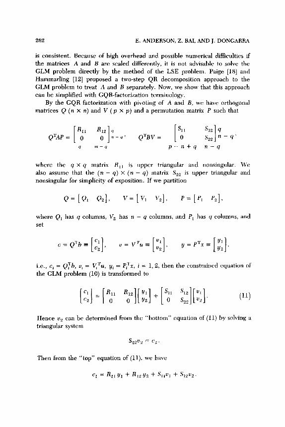
is consistent. Because of high overhead and possible numerical diffkulties if the matrices A and B are scaled differently, it is not advisable to solve the GLM problem directly by the method of the LSE problem. Paige [lS] and Hammarling [12] proposed a two-step QR decomposition approach to the GLM problem to treat A and B separately. Now, we show that this approach can be simplified with GQR-factorization terminology.

By the GQR factorization with pivoting of A and B, we have orthogonal matrices Q (n x n) and V ( p x p) and a permutation matrix P such that

Y m-q p-n+9 n-q

where the 9 x 9 matrix R,, is upper triangular and nonsingular. We also assume that the (n - 9) x (n - 9) matrix S,, is upper triangular and nonsingular for simplicity of exposition. If we partition

Q= [Ql a,]> v=[% Vz], p=[p, P2],

where Q, has 9 columns, V, has n - 9 columns, and P, has 9 columns, and set

“=vTuE Vl [ 1 “2 ’

i.e., ci = QTb, vi = ViTu, yi = PiTx. i = 1,2, then the constrained equation of the GLM problem (10) is transformed to

Cl [I [ R = 11

c2 0

Hence v2 can be determined triangular system

from the “bottom” equation of (11) by solving a

s22v2 = c2.

(11)

Then from the “top” equation of (ll), we have

CI = R,,Y, + R,,Y, + S,,v, + %2v2.


It is obvious that to get the minimum-2-norm solutions, the remaining compo-

nents of the solutions can be chosen as

“1 - - 0, yz = 0, Yl = Kl’(c, - wz).

Then the solutions of the original problem are

x, = f’&(QT - S,,S,‘Q~)b, u, = V,S,‘Q;b.

EXAMPLE. Let the matrices A, B and the vector b in the GLM problem

1.; -j -; -j _j, R=[-i j -;!, b=[j

where rank( A) = 3, rank(B) = 2. The exact solutions of the GLM problem are

X, = i[O, 6,10, - 161T and U, = &[14, 70, 281T.

By the GQR factorization with column pivoting of the matrices A and B, we have

I

-4.4721 - 1.3416 - 1.3416 0 -3.4928 - 6.2986

R= 0 0 1.6743 0 0

0.3111

[ 1 1.5556 . 0.6222

Then the computed solutions are

[

0

2, 0.6667 = = 2.1111 1 ’ ue A

- 1.7778


The relative errors of the computed solutions are

II x&? - %?I12 II%? - %.lI, = -

II %.I1 2 7.9752 x

10-16, II 6.6762 x 10-16.

ut? II 2

The square minimal length of the vector ii, is &z&, = 2.9037, and the residual is )I b - Af, - I?&,)( 2 = 4.4464 x 10-l’.

The Sensitivity of the GLM Problem. Regarding the sensitivity of the problem to perturbations, we shall consider the effects of the perturbations in the vector b and in the matrices A and B. Let the perturbed GLM problem be defined as

min CTiTu 4, ii

subjectto b+e= (A+E)Z+(B+F)u.

The solutions are denoted by Xe and E,. Then under the assumptions

rank(A) = rank( A + E) = m

and

rank( A, B) = rank( A + E, B + F) = n,

we have the following bounds on the relative error in 2, and li, due to the perturbations of b, A, and B:

GLM-Problem Perturbation Bounds.

II ze - xell

II xe II

+‘%(A)

and

II% - %?lI II EII II B II II PII

Ii b II ’ KB(A) II All llbll

II P II + lIFll((b(l + O(E2)> (13)


where

KB( A) = II All II &I. “A(B) = llBil ll(GB)+ll~

G = Z - AA+, AL = At[Z - B(GB)+], and p = [GZ3(GB)T]tb, Fl = FBT + BFT.

Here O(E’) represents the higher-order term in the perturbation matrices E, F, etc.

The proof is long and appears in the appendix. If we note that

lIfwl1 Pll Q eqqll4~

then the bounds (12) and (13) can be simplified. We see that the sensitivities of 5, and U, basically depend on K~( A) and K*(B). For this reason, K~( A)

and K~( B) are defined as the condition numbers of the GLM problem. They can be used to predict the effects of errors in the regression variables on regression coefficients.

As a special case, we note that if B = I, then the GLM problem is reduced to the classical linear regression problem. Then u, is just the residual vector, u,=r,=b-Ax,,ii,=r,=(b+e)-(A+E)?,,F=O,and

KB( A) = K(A) = II All II A+lL K*(B) = 1.

Hence we have

II Te - x,II IIEII IIf-t?ll II x II + K2(A) 1) AlI )I AlI II x,1/ + ‘(‘“)

and

II Fe - rf?ll IJEll IIr,lI II Tell Ilell -- II bll gK(A)mIJbll + llE” Ilbll + Ilbll + Ok”)

These are the well-known perturbation results for the solution and residual of the ordinary linear regression problem [22, lo].

Estimation of Condition Numbers. To estimate the condition numbers Kg(A) and K~( B) of the GLM problem, we again can use the Hager-Higham method without the expense of forming At or (GB)+. By this technique, the required vector norms ]I Kz 11 o can be computed from the GQR factorization


of A and B, where K = (GB)+ or K = AL and z > 0 is a vector that is readily computed. After tedious computations, we have

(GB)+z = V,S,‘Q;z

ALz = P,R,‘(QTz - S,,S,'Q~z).

Hence, we can just use a triangular system solver and matrix-vector operations to give the estimation of condition numbers of the GLM problem.

Roughly speaking, we see that the conditioning of the GLM problem depends on the conditioning of the triangular matrices II,, and S,,.

4.3. Other Applications

In this section, we briefly mention some other applications of the GQR factorizations.

The GQR factorization has been used as a preprocessing step for computing the generalized singular-value decomposition in the Jacobi-Kogbetliantz approach; see Paige [19] and Bai [2].

The GQR factorization can also be used in solving structural equations:

f = A=t, e = BBTt, e= -Ad,

where f is given, and we wish to find d. This kind of problem regularly arises in the analysis of structures made up of elements joined in the style of a framework or network; see Heath et al. [13] and Paige [20].

5. SUMMARY AND FUTURE WORK

In this paper, we have defined the generalized QR factorization with or without partial pivoting of two matrices A and B, each having the same number of rows, and shown its applications in solving the linear equality- constrained least-squares problem and generalized linear model problems, and in assessing the conditioning of these problems. A similar development could be done for matrices A and B having the same number of columns, instead of the same number of rows. Then the GQR factorization of A and B would be equivalent to the QR factorization of AB-‘. These discussions have served as the guideline for our future development of GQR factorization software for the LAPACK library [l].


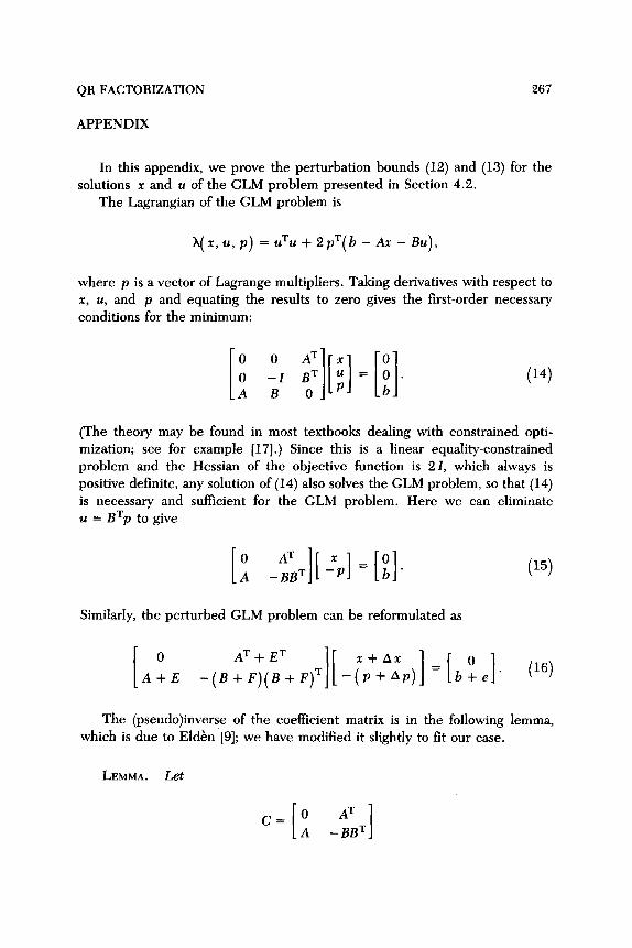
APPENDIX

In this appendix, we prove the perturbation bounds (12) and (13) for the solutions x and u of the GLM problem presented in Section 4.2.

The Lagrangian of the GLM problem is

h(x,u, p) = uTu + 2p’(b - Ax - “),

where p is a vector of Lagrange multipliers. Taking derivatives with respect to x, U, and p and equating the results to zero gives the first-order necessary conditions for the minimum:

(The theory may be found in most textbooks dealing with constrained optimization; see for example [17].) S ince this is a linear equality-constrained problem and the Hessian of the objective function is 2 I, which always is positive definite, any solution of (14) also solves the GLM problem, so that (14) is necessary and sufficient for the GLM problem. Here we can eliminate u = BTp to give

Similarly, the perturbed GLM problem can be reformulated as

0

A+E AT+ET T][ -;p+:;p)] = [,!.I. (16) -(B + F)(B + F)

The (pseudo)inverse of the coefficient matrix is in the following lemma, which is due to Elditn [9]; we have modified it slightly to fit our case.

LEMMA. Let

268

and

E. ANDERSON, Z. BAI, AND J. DONGARRA

AtB

1 GT[(GB)(GB)T]+G ’

where

G=I-AA+, AL = A+[ I - B(GB)+] .

If rank([ A, B]) = n then Y = Ct. Further, if A has full column rank, then , Y = c-l.

Subtracting the matrix equation (15) from (16), we have

= -(C+Ec)-‘E,[;] + (C+E,)-‘[;I, (17)

where

Ec= ; ET

[ 1 _F ) Fl = FB= + BF=.

1

If l)CPIE,)) < 1, then we can make the expansion

(C+E,)-‘= C-l _ C-lE,C-’ + . . . ,

and then (17) becomes

-C-‘E,[ ;] + C-‘[ o] + O(E”),

where O(E’) means the higher-order terms in the perturbation factors E, and e, which we omit in the formulas that follow. By the lemma, we have

After taking norms, it becomes

IlAx 11 G II BII’ II ALlI’ II EII II PII + II ALll( II EII II x II + II F,\l II PI\ + \I ell) .

QR FACTORIZATION

Using the condition numbers

269

we get the desired relative perturbation bound (12) on the solution x.

For the perturbation bound on the solution u, from (IT), we first have

Ap = -( AL)TETp + GT[(GB)(GB)T]+G(~~ + F,p + e).

Since u = BTp and u + Au = (B + F)T( p + A p), we have, subtracting them and using At = AT( AAT)+,

Au = BTAp + Fp

= B’( AL)TETp + BTGT [(GB)(GB)~]+G(E~ + F,~ + e)

= BT( AL)TETp + ( GB)+G( EX + FI p + e),

where the higher-order terms of the perturbation factors of E, F, and e again

are not presented. By taking norms, and substituting in the condition numbers K e(A) and K A(B), we get the desired perturbation bound (13) on the solution u.

The authors are very grateful to Jim Demmel, Sven Hammarling, and Jeremy Du Croz for their valuable comments. special thanks to the referees, whose presentation.

REFERENCES

E. Anderson, Z. Bai, C. Bischof, J. Demmel, J. Dongarra, J. Du Croz, A. Greenbaum, S. Hammarling, A. McKenney, and D. Sorensen,

LAPACK: A portable linear algebra library for high performance comput- ers, in Proceedings Super-computing ‘90, IEEE Computer Sot. Press, Los

Alamitos, Cahf., 1990, pp. 2-11. Z. Bai, An improved algorithm for computing the generalized singular value decomposition, Numer. Math., submitted for publication. J. L. Barlow, N. K. Nichols, and R. J. Plemmons, Iterative methods for

equality constrained least squares problems, SIAM]. Sci. Statist. Comput. 9:892-906 (1988).

The authors would also like to express comments led to improvements in the


4

5

6

7

8

9

10

11

12

13

14

15

16

17

18

19

20

J. L. Barlow, Error analysis and implementation aspects of deferred correction for equality constrained least squares problems, SZAM J. Numer. Anal. 25:1340-1358 (1989). C. H. Bischof and P. C. Hansen, Structure-Preserving and Rank-Reveal- ing QR-Factorizations, Preprint MCS-PlOO-0989, Argonne National Lab., 10989. Ake Bjorck, Least squares methods, in Handbook of Numerical Analysis.

Vol. 1: Solution of Equations in R” (P. G. Ciarlet and J. L. Lions, Eds.), Elsevier North Holland, 1987. T. F. Chan, Rank revealing QR factorizations, Linear Algebra A&. 88/89:67-82 (1987). J. J. Dongarra, J. R. Bunch, C. B. Moler, and G. W. Stewart, LZNPACK

User's Guide, SIAM, Philadelphia, 1979. L. Elden, Perturbation theory for the least squares problem with linear equality constraints, SZAM J. Numer. Anal. 17:338-350 (1980). G. H. Golub and C. F. Van Loan, Matrix Computations, Johns Hopkins U.P., Baltimore, 1989. W. W. Hager, Condition Estimates, SIAM J. Sci. Statist. Comput.

31(2):221-239 (1984). S. Hammarling, The numerical solution of the general Gauss-Markov linear model, in Mathematics in Signal Processing (T. S. Durrani et al., Eds.), Clarendon Press, Oxford, 1986. M. T. Heath, R. J. Plemmons, and R. C. Ward, Sparse orthogonal schemes for structural optimization using the force method, SZAM J.Sci.

Statist. Comput. 7:1147-1159 (1984). N. J. Higham, FORTRAN codes for estimating the one-norm of a real or complex matrix, with applications to condition estimation, ACM Trans.

Math. Software 14:381-396 (1988).

S. Kourouklis and C. Paige, A constrained least squares approach to the general Gauss-Markov model, J. Amer. Statist. Assoc. 76:620-625

(1981). C. L. Lawson and R. J. Hanson, Solving Least Squares Problems, Pren- tice-Hall, Englewood Cliffs, N.J., 1974. D. G. Luenberger, Linear and Nonlinear Programming, 2nd ed., Addison-Wesley, Reading, Mass., 1984. C. Paige, Computer solution and perturbation analysis of generalized linear least squares problems, Math. Comput. 33:171-183 (1979). C. Paige, Computing the generalized singular value decomposition, SIAM J. Sci. Statist. Cornput. 7:1126-1146 (1986). C. Paige, Some aspects of generalized QR factorization, in Reliable

Numerical Computations (M. Cox and S. Hammarling, Eds.), Clarendon Press, Oxford, 1990.


21 R. Schreiber and C. Van Loan, A storage effkient WY representation for

products of Householder transformations, SlAM /. Sci. Statist. Comput.

10(1):53-57 (Jan. 1989). 22 G. W. Stewart, On the perturbation of pseudo-inverses, projections and

linear least squares problems, SIAM Reu. 19:634-662 (1977). 23 C. F. Van Loan, On the method of weighting for equality-constrained

least-squares problems, SlAM J. Numer. Anal. 22:851-864 (1985).

Received 31 July 1990; final manuscript accepted 6 March 1991

generalized qr factorization and its applications* e

Documents