AFRPL TR-85-066 AD:

Final Report N n R a tn u b ln

\Novemberl1979 to Mixing Experiments-~August 1985

PLEASE REPLACE TH rFRONT ~VRAND DD 14173 OF AMRLT8O 6 WT H

~~ ATTACEDRVISION.

September 1935 Author: Calspan. Advanced Technology CtrC. Padova P.O. Box 400

Buffalo, New York 14225

6632-A-Rev. 1F0461 1-80-0-001 1

Approved for Public Relgase

Distribution is unlimited. The AFRPL Technical Services Off Ice has reviewed this report, and It Isreleasable tothe National Technical Information Service, whene it will be availabl, to the generalpublic, Including foreign nationals.

proepared for the: Air ForceRocket PropulsionLaboratoryAir Force Space Technology CenterSpace Division, Air Force Systems Command

Reproduced From Edwards Air Force Base,Best Available Copy California 93523-5000

NOTICE

When U.S. Government drawings, specifications, or other data are used for any purposeother than a definitely related Government procurement operation, the Governmentthereby incurs no responsibility nor any obligation whatsoever, and the fact that theGovernment may have formulated, furnished, or in any way supplied the said drawings,specifications, or other data is not to be regarded by implication or otherwise, or in anymanner licensing the holder or any other person or corporation, or conveying any rights orpermission to manufacture, use or sell any patented invention that may in any way berelated hereto.

FOREWORD

The Air Force Rocket Propulsion Laboratory is pleased to publish this report forcontract F04611-90-C-0011 for use by its contractors and other workers studying theturbulent mixing of supersonic co-flowing jets. The data presented here are unique interms of the range of test variables and spatial extent. Prior to publication, these datawere analyzed for consistency by a member of the AFRPL advisory panel, Mr. R. Rhodes(CPIA Publication 384, Vol. II, p. 157+). It was found that the velocity and concentrationprofiles deduced from this data are reasonably consistent; however, the variation of thederived centerline properties such as velocity are not as well behaved as we would likethem to be. This behavior of the derived quantities is thought to be at least partially anartifact of the data interpolation techniques used to estimate the value of the measuredvariables on a common computational grid. Another source of apparent scatter is theboundary layer behavior of the experimental device. Pergament (SAIC/PR TM-26, June1984) found that the data correlation markedly improved when a proper description of thenozzle boundary layers was used as input in his finite difference modeling code.Unfortunately, a formal error analysis i not included in this report due to fiscal andcontractor personnel availability limitations. We regret this omissicn and caution theserious user to peruse these two referenced reports to get an indication of the consistencyof the data. These cautionary comments are made to encourage potential users of thisdata to perform as thorough an analysis of the data as the complexity of the experimentconfiguration requires.

We wish to thank the principle investigator, Dr. Corso Padova of the Arvin CalspanCorporation, for his dedication and diligence. This report literally could not have beenwritten without his insight into the experimental program and his extra personal effort toproduce a quality final report.

This technical report has been reviewed and is approved for publication anddistribution in accordance with the distribution statement on the cover and on the DDForm 1473.

PHILIP A.VESSEL L. KEVIN SLIMAKProject Manager Chief, Interdisciplinary Space

Technology Branch

FOR THE DIRECTOR

HOMER M. PRESSLEY JR., Lt CliSAFChief, Propulsion Aralysis Division

SECURITY CLASSIFICATION OF THIS PAGE

REPORT DOCUMENTATION PAGE

Is REPORT SECURITY CLASSIFICA1 ION 1b. RESTRICTIVE MARKINGS

UNCLASSIFIED _

2.. SECURITY CLASSIFICATION AUTHORITY 3. DISTRIBUTION/AVAILABILITY OF REPORT

Approved for Public Release; Distribution is

2b. OECLASSIFICATION/DOWNGRADING SCHEDULE limited.

PERFORMING ORGANIZATION REPORT NUMBERIS) 5. MONITORING ORGANIZATION REPORT NUMBER(S)

6632-A-3-Rev. 1 AFRPL-TR-85-066

6s NAME OF PERFORMING ORGANIZATION 6b. OFFICE SYMBOL 7a. NAME OF MONITORING ORGANIZATION

Calspan Advanced Technology (I(.pplicabte

Center Air Force Rocket Propulsion Laboratory

6c. ADDRESS (City. State and ZIP Code) 7b. ADDRESS (City. Slate and ZIP Code)

P.O. Box 400 AFRPL/DYSO (Stop 24)

Buffalo NY 14225 Edwards AFB CA 93523-5000

So NAME OF FUNDING/SPONSORING 8b. OFFICE SYMBOL 9. PROCUREMENT INSTRUMENT IDENTIFICATION NUMBER

ORGANIZATION (if opplable) I

AFRPL DYSO F04611-80-C-0011

Sc. ADDRESS (City. State and ZIP Code) 10. SOURCE OF FUNDING NOS.

Stop 24 PROGRAM PROJECT TASK WORK UNIT

Ea AF C ELEMENT NO. NO. NO. NO.

62302F 3058 10 VK11 TITLE (Include Se;curity Clasification)62

0F3510V

Non-Reacting Turbulent Mixing .Experiments (U),

12. PERSONAL AUTHOR(S)

Padova, Corso13. TYPE OF REPORT 13b. TIME COVERED 14. DATE OF REPORT (Yr.. Mo.. Dayi 15. PAGE COUNT

Final FROM TO n:/Og 85/9 166

ii. SUPPLEMENTARY NOTATION

Additional Cosati code 21 08

17. COSATICODES 13. SUBJECT TERMS (Continue oil rvverae if neeesuary and lat.ntify by block number)

FIELD GROUP SUS. GR. turbulent mixing, axisymmetric jets, co-flowing jets, super-

05 sonic jets, turbulence modeling, rocket exhaust plumes16 04

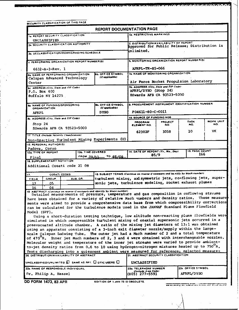
19. ABSTRACT IWonflnut on reuerse i( neceaar, and Identify by blocs numbertDetailed measurements of pressure, uemperatura and gas composition in coflowing streams

have been obtained for a variety of relative Mach numbers and density ratios. These measure

ments were aimed to provide a comprehensive data base from which compressibility corrections

can be calculated for the turbulence models used in the JANNAF Suandard Plume Flowfield

Model (SPF).Using a short-duration testing technique, low altitude non-reacting plume flowfields were

simulated in which compressible turbulent mixing of coaxial supersonic jets occurred in a

preevacuated altitude chamber. A ratio of the mixing jet diameters of 13:1 was obtained

using an apparatus consisting of a 3-inch exit diameter nozzle/supply within the large-

scale Calspan Ludwieg Tube. The outer jet had a Mach number of 2 and a total temperature

of 470 0 R. Inner jet Mach numbers of 2, 3 and 4 were obtained with interchangeable nozzles.Molecular weight and temperature of the inner jet streams were varied to provide ambient-

to-jet density ratios from 0.6 to 10 using hydrogen-nitrogen mixtures heated up to 7500R.

Tests discharging into a quiescent ambient were measured for reference: selected measure-20. DISTRIBUTION/AVAILABILITY OF ABSTRACT 21. ABSTRACT SECURITY CLASSIFICATION

UNCLASSIFIED/UNLIMITED 9 SAME AS APT. 0 DTIC USERS 0 UNCLASSIFIED

22a. NAME OF RESPONSIBLE INDIVIDUAL 22b. TELEPHONF NUMBER 22c OFFICE SYMBOL(Include Ato Code)

Dr. Philip A. Kessel (805) 277-5591 AFRPL/DYSO

DO FORM 1473, 83 APR EDITION OF I JAN 73 IS OBSOLETE.

SECURITY CLASSIFICATION OF THIS PAGE

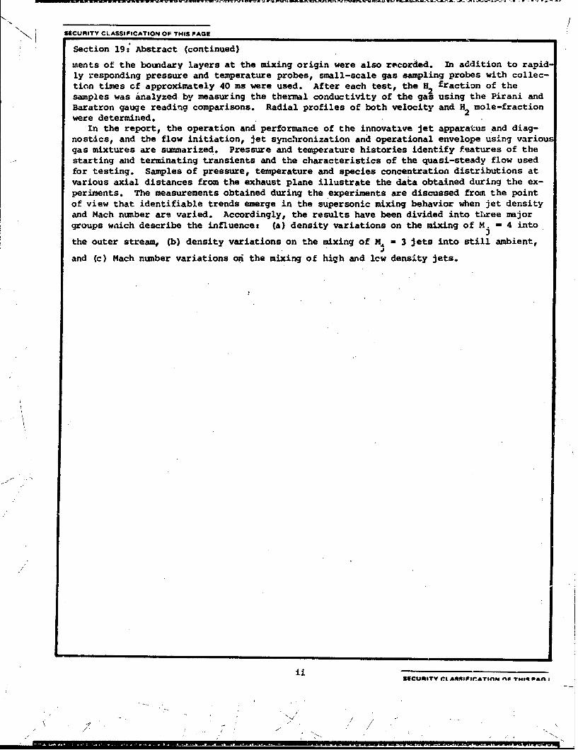
Section 19: Abstract (continued)

ments of the boudary layers at the mixing origin were also recorded. In addition to rapid-ly responding pressure and temperature probes, small-scale gas sampling probes with collec-

tion times cf approximately 40 ms were used. After each test, the H fraction of thesamples was analyzed by measuring the thermal conductivity of the gas using the Pirani andBaratron gauge reading comparisons. Radial profiles of both velocity and H2 mole-fractionwere determined.

In the report, the operation and performance of the innovative jet apparatus and diag-nostics, and the flow initiation, jet synchronization and operational envelope using v.riougas mixtures are summarized. Pressure and temperature histories identify features of thestarting and terminating transients and the characteristics of the quasi-steady flow usedfor testing. Samples of pressure, temperature and species concentration distributions atvarious axial distances from the exhaust plane illustrate the data obtained during the ex-periments. The measurements obtained during the experiments are discussed from the pointof view that identifiable trends emerge in the supersonic mixing behavior when jet densityand Mach number are varied. Accordingly, the results have been divided into t*ree majorgroups waich describe the influence: (a) density variations on the mixing of M. - 4 into

Jthe outer stream, (b) density variations on the mixing of M, - 3 jets into still ambient,

Jand (c) Mach number variations on the mixing of high and lcw density jets.

i SECitUITYf C LA**iIIEII'ATII 'lj f l lll ?M I .A *

x/' /' 7

FOREWORD

Calspan has conducted a series of non-reacting turbulent jet mixing

experiments utilizing innovative short-duration test techniques and fast-acting

diagnostics. This program, under the sponsorship of the Air Force Rocket Pro-

pulsion Laboratory (AFRPL), covered a 36 month period from 1979 to 1982.

The experiments were conducted in separate phases that furnished the

Air rorce with milestones and decision gates before each succeeding phase.

A very close liaison withthe Air Force technical monitors, T. Dwayne McCay,

A. Kawasaki and P. Kessel, existed thrcughout the program. In addition,

frequent technical-direction meetings were held with the RPL Advisory panel

consisting of T.D. McCay (RPL and later NASA Marshall), H. Pergament (SAI),

B. Walker (Army Missile Commnnd), G. Brown (Cal Tech), A. Roshko (Cal Tech),

and R. Rhodes (ARO, AEDC).

The technical activity was detailed in monthly progress reports

in addition to the Technical Direction meetings. Several reports were published

during the program in which experimental data were submitted to AFRPL on a timelybasis.

The program was conducted by the Aerodynamic Research Department at

Calspan, utilizing a number of key technical people as part of the experimental

team. The effort was initially led by C. E. Wittliff. Subsequent phases

of the program were completed under the direction of C. Padova. Additional

contributors were W. Wurster and D. Boyer in the areas of fast-acting diagnostics,

data analysis and experimental techniques, and P. Marrone in data analysis and

program direction. The efforts of R. Bergman, S. Sweet, M. Urso, C. Bardo,

F. Urso and R. Hiemenz were also central to the success of the program.

The reports which were released as part of this effort are listed below:

1. Non-Reacting Turbulent Mixing Experiments CDRL Item 1, 8 January 1980,

"Program Plan" Submitted by C. E. Wittliff.

2. Calspan Report No. 6632-A-1, 25 July 1980, "Phase I Test Report"

Submitted by C. E. Wittliff.

Jiii

3. Non-Reacting Turbulent Mixing Experiments, August 1981, "Phase 0 Test

Report" Submitted by C. Padova and W. H. Wurster.

4. Tubulent Mixing Experiments, 18 November 1981, "Illustrative Raw Data from

Phase 1/81 Tests" Submitted by C. Padova.

5. Non-Reacting Turbulent Mixing Experiments, 20 November and 3 December 1981,

"Phase 1/81 Data Package (and Supplementary D.P.)" Submitted by C. Padova.

6. Calspan Report No. 6632-A-2, August 1982, "Phase II - Test Engineering

Report" Submitted by C. Padova.

7. Calspan Report No. 6632-A-2, September 1982, "Phase II - Test Engineering

Report. Supplement No. 1 - Data Plots" Submitted by C. Padova.

iv

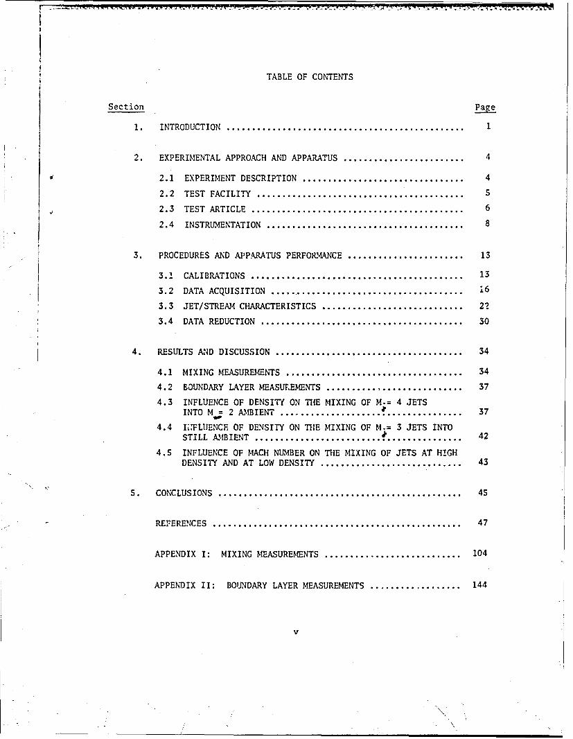
TABLE OF CONTENTS

Section Page

1. INTRODUCTION ............................................... 1

2. EXPERIMENTAL APPROACH AND APPARATUS ........................ 4

2.1 EXPERIMENT DESCRIPTION ................................ 4

2.2 TEST FACILITY ......................................... S

2.3 TEST ARTICLE .......................................... 6

2.4 INSTRUMENTATION ....................................... 8

3. PROCEDURES AND APPARATUS PERFORMANCE ....................... 13

3.1 CALIBRATIONS .......................................... 13

3.2 DATA ACQUISITION ....................................... 16

3.3 JET/STREAM CHARACTERISTICS ............................ 22

3.4 DATA REDUCTION ........................................ 30

4. RESULTS AND DISCUSSION .......... .......................... 34

4.1 MIXING MEASUREMENTS ................................... 34

4.2 BOUNDARY LAYER MEASUREMENTS ........................... 37

4.3 INFLUENCE OF DENSITY ON THE MIXING OF M.= 4 JETSINTO M = 2 AMBIENT .......... o ........................ 37

4.4 I2.FLUENCE OF DENSITY ON THE MIXING OF M.= 3 JETS INTOSTILL AMBIENT ......................................... 42

4.5 INFLUENCE OF MACH NUMBER ON THE MIXING OF JETS AT HIGHDENSITY AND AT LOW DENSITY ............................ 43

S. CONCLUSIONS ................................................ 45

REFERENCES ................................................. 47

APPENDIX I: MIXING MEASUREMENTS ........................... 104

APPENDIX II: BOUNDARY LAYER MEASUREMENTS .................. 144

V

LIST OF FIGURES

\Figure Page

1 Calspan Ludwieg Tube Wind Tunnel .............................. 57

2 Schematic of Jet Mixing Experiment ........................... 58

3 Ludwieg Tube Facility Configuration for Turbulent Mixing

Experiments .................................................. 59

4 Schematic of Jet System ...................................... 60

5 Views of the Apparatus ....................................... 61

6 Nozzle Contours .............................................. 62

7 View of the Instrumented Rake for Mixing Surveys ............. 63

8 View of the Probes for Gasdynamic Measurements ............... 64

9 Schematic of Heat Conductivity Gas Sampler System ............ 66

10 View of the Probes for Gas Sampling .......................... 67

1! Response to Water Immersion of a Temperature Probe ........... 68

12 Response of the Temperature Probes in the Jets at VariousCompositions and Levels of Dynamic Pressure .................. 69

13 Influence of Gas Composition on the Measurement of PressureUsing Pirani and Baratron Gauges ............................. 71

14 Gas Samuler Calibration ...................................... 72

15 Pre-test Monitoring of Reference Temperatures ................ 73

16 Histories of Flow Variables Measured in the Mixing Region .... 74

17 Sample of Averaged Data from the DDAS ........................ 75

18 Histories of Flow Variables Illustrating the Jet/StreamCharacteristics .............................................. 77

19 Synchronization of the CLT and Jet Discharges ................ 78

20 Histories of Plenum Pressure for M. 4, 3, 2 Jets ............. 79

21 Histories of Jet Variables in a Heated-Jet Test Case ......... 80

22 Radial Variation of the Measurements in a Typical No-WindTest Case .................................................... 81

1 viNt

: ., , / •,. .1'':

LIST OF FIGURES (Cont'd)

Figure Page

23 Radial Variation of the Measurements in a Typical Wind-OnTest Case ...................... .............................. 86

24 Reproducibility of the Data ................................... 92

25 Comparison of Radial Pitot Pressures with and without CLTNozzle Extension .............................................. 93

26 Illustrative Test Run Summary ................................. 94

27 Illustrative Calculation of Radial Velocity Profile ........... 95

28 Variation of Jet Composition from Nea to Far Field.M. = 4 Jet Discharging into the Strjersonic Stream WithDnsity Matched ..................... ............................ 96

29 Variation of Pitot Pressure from Near to Far Field.M. a 4 Jet Discharging into the Supersonic Stream Wit.Dinsity Matched .................. ............................ 97

30 Velocity Variations frm Near to Mid Field.M. - 4; Mae - 2; Density Matched ............................. 98

31 Influence of Density Variations on Velocity Surveys at 40 R..j 4., Meo= 2 ................................................. 99

32 Axial Decay of Jet Core Composition ......................... 100

33 Influence of Density Vafiations on Core LengthM . 4, Mao 2 ............................................... 101

34 Pitot Pressure and Composition Profiles in the Mixi-Z Jetat 20 R.. M. = 3 Jet Discharging into Still Ambientwith JDensily Matched ...................................... 102

35 Composition Profile in the Mixing Jet at 20 R..M. - 2 Jet Discharging into Still Ambient J3with = 0.6 ........................................ 103

vii

K

• . \\ --

LIST OF TABLES

Table Page

I Nozzle Coordinates ......................................... 48

II Specifications for Hydrogen/Nitrogen Gas Mixtures ........... 49

III Matrix of Test Cases ....................................... so

SIV Completed Data Points ...................................... 51

V Data Points Surveying the Nozzle Boundary Layers ........... 52

VI Measured Nozzle Parameters ................................ 53

VII Initial and Reference Parameters for the Mixing* Measurements ............................................... S4

VIII Initial Velocities and Actual Density Ratios tor theMixing Measurements ....................................... 56

viii

.f m~ Kr lo- -Um

12IST OF SYMBOLS

BL, GP. S Designation L.)de for the diagnostic probes (as identified in

T, RC, TR the text at page 19)

M Mach number

MW Molecular weight

P Static pressure in the flow field

P i Initial (pre-test) pressure in the charge tube of the jet or

outer stream (CLT)

P Stagnation pressure>9a

P0 Pitot pressure

R Universal gas constant

R. Radius at the exit plane of the Jet

Ti Initial (pre-test) temperature in the charge caie of the jet

or outer stream (CLT)

TO Stagnation temperature

U Axial component of velocity

X Axial distance measured from the jet exit plane

XP2 XN Mole fractions of Hydrogen and Nitrogen

Y, Z Horizontal and vertical reference axes with origin at the center

of the cruciform probe holder

ix

,r-- , -- _± : --.. L . ..- lrwin-"ur ,r

Local gas density

' Ratio of specific heats

SUBSCRIPTS

. c at centerline in the mixing region

Co core of the jet

ct in jet charge tube, upstream of venturi throat

* ref ambient level in the test chamber prior to jet initiation

j relative to the jet

relative to the ambient surrounding the jet

COMPUTER SYMBOLS USED IN THE TABULATIONS OF APPENDIX I

MA, XJ, M.J, PO, P, R, RHA/RHJ, U, X/RJ, XH12

All as identified in the text at page 30

x

Section 1

INTRODUCTION

Research on supersonic jet mixing, especially in '-he area of low-altitude

rocket exhaust-plume technology, has been a critical part of the Air Force

Rocket Propulsion Laboratoy (AFRPL) program for seve'al years. A major objective

has been thedivelopment of computer codes for the prediction of plume observables,

such as the radiation signature. These codes nedel complex physical and chemically-

reactive flowfields. In the gasdynamic computations, modeling the turbulent

transport procebses remains as a major obstacle to a useful and widely appli-

cable analysis of free turbulent flow phenomena. Work on this aspect is actively

in progress. Advances in computational fluid dynamics have essentially offset

the theoretical difficulties which constrained the complexity of the modeling

approach up to the mid 1960s. These methods have been exercised on complex

problems by using exact implementations of classical turbulence models and by

developing new models to improve predictive power. In the course of this

process, not surprisingly, a renewed need for experimental data has emerged

to be used in the evaluation of the computational alternatives.

A case in point is the JANNAF-sponsored effort to develop an industry-

standard gasdynamic model for low-altitude plumes. The turbulence module of the

JANNAF Standard Plume Flow-Field (SFF) code I has five alternate turbulence

models to predict the mixing phenomena that influences the development of exhaust

plumes. They range from the simple traditional algebraic models to the advanced

two-equation models, and they can be used in compressibility-corrected versions

of the code that should imprcve the calculations of flow fields containing large

density gradients.

In support of low-altitude plume research, AFRPL-sponsored experimental

programs have been performed at AEDC and Calspan ATC. In general, the experiments

were designed primarily to investigate the structure of the plume and its

emitted radiation, often for particular propellant combinations, motor

configurations and ambient conditions (i.e., Mach number and altitude).

I

Detailed information on the turbulent mixing phenomena is liot readily discernible

from these test data because of the complicating factors of the "real" plume.

Recently, in response to the projected need to corroborate the SPF code, Calspan

has defined a different experimental approach. The key concept of the approach

is to use a unique short duration technique that is flexible enough to sequentially

investigate, in a building block fashion, several of the physical and chemical

complexities of low altitude plumes. Specifically, the technique would first

be used to measure parameters such as density, Mach number and exit pressure

in non-reacting jets over a broad range of gasdynamic conditions. Then the

technique would be extended to mixing jets with "real" plume features also

using basically the same controlled laboratory situation. These measurements

would include having either or both jets laden with solid particulates and re-

acting mixtures combined with subtantially an unaltered capability to control

the gasdynamic parameters.

This report describes the results of the Calspan experimental program,

sponsored by AFRPL, to investigate the supersonic mixing phenomena in the

fundamental non-reacting jets case. The short duration approach outlined above

was developed and applied to obtain these results. A primary objective of

this experimental study was to generate a firm and comprehensive data base I

from which to select and establish compressibility corrections for the turbulence

models of the JANNAF SPF. Within this framework, the needs for a fundamental

description of the supersonic mixing phenomena were re-examined in the initial

discussions with AFRPL. The influence of Mach number and density ratios were

identified as the foremost gap to be filled. Fundamental measurements of

turbulent mixing go back many years, and comprehensive reviews of experimental2,3data are available. However, previous studies are scarce and most con-

centrate on specific and unrelated cases, especially in the range of Mach

numbers above 2 and plume densities well below or well above ambient. Thus,

experiments with non-reacting jets at Mach numbers of 2, 3 and 4 and ambient-

to-jet density ratios from 0.6 to 10 were identified as having the highest po-

tential of yielding the data needed to support the use and future development

2i

of tl.; SPF. Experiments with jets discharging both in a Mach 2 outer stream

and in a quiescent ambient were judged important for their applications and for cor-

relations with existing data. Mixing measurements over the above range of conditions

were completed recently and are presented in this report.

Following this introduction, Section 2 briefly describes the Calspan

test facility used. In the same section, the jet apparatus and the fast-response

diagnostics which were designed especially for the experiments are reviewed in some

detail. The prccedures to obtain these mixing data are presented in Section 3

with a general description of the measured characteristics of the jets and outer

stream. In Section 4, the extensive measurements of pressure, temperature, and

gas species which describe the mixing of the jets are discussed. The mean ve-

locities computed from the measurements are also presented to indicate how the

Mach nubmer and density variations influence the mixing'process. The actual

measurements are tabulated in Appendix I; plots of the measurements were

iublished earlier (Reference 4).

Section S presents a precis of the main observations derived from the

experimental investigation. Theysupport these overall conclusions:

* well resolved measurements of gas species and velocity profiles

have been obtained for a variety of Mach numbers and density

ratios;

* these measurements expand the data base needed to support the

ongoing turbulence modeling effort; and

0 the short duration technique developed for the measurements

represents a valuable tool for investigating fundamental plume

phenomena over a broad range of experimental conditions.

3

Section 2

EXPER:MENTAL APPROACH AND APPARATUS

2.1 EXPERIMENT DESCRIPTION• 5,6

A unique short-duration testing technique was developed at Calspan

to study the supersonic mixing phenomena. The approach is especially suited

to the broad range of test conditions of interest and for its zpplication to

reacting plume neasurements. The technique is based on the capabilities of

the large-scale Calspan Ludwieg Tube (CLT) wind tunnel, depicted in Figure 1.

Using this facility, an experiment was configured as sketched in Figure 2. A

jet of arbitrary gas composition, a few inches in diameter at its origin, was

exhausted into an essentially unconfined ambient which could simulate a wide

range of altitude conditions. The ambient surrounding the jet was either still

or moving at supersonic speeu. A key operating characteristic of the CLT is

permitted control of gas species in both the jet and the freestream flow to

meet the demanding experimental requirements. Specific r-,Ibinations of various

gases were used to achieve a broad range of density ratios. In addition, for

flow diagnosis, freestream and jet gases with the same composition were tagged

with a trace amount of suitable gas additive. For each of the mixing flow fields

that were generated, the measurements consisted of radial surveys r" the jet

plume at selected axial stations downstream of the exit plane. Because of the

large scale of the jets, their mixing could be probed in detail with diagnostics

simultaneously measuring pitot and static pressures, temperature, and gas

species.

The flexibility of the short-duration testing approach for supersonic

mixing measurements is apparent from the experimental conditions used in the

Calspan investigation. Their range is indicated in Figure 2. The conditions were

selected to separately evaluate the effects of freestream-to-jet density ratio,

jet Mach number and freestream Mach number. The three jet Mach numbers, Mj, of

2,3, and 4 were produced by interchangeable nozzles. The molecular weight, mwj,

and stagnation temperature, Toj, of the jets were varied to span values of the ambient-

to-jet density ratio, PZp , from 0.6 to 10. This was achieved by using

hydrogen-nitrogen mixtures heated as high as 8000R. The ambient, in which the

4

jet discharged was either quiescent (no-wind cases) or flowing at Moo= 2 (wind-on

cases), had a stagnation temperature, To 0,, at or below ambient as determined

by the operating characteristics of the CLT. In keeping with the overall purpose

of generating a fundamental data base, complicating factors which characterize

"real" low altitude plumes, such as a repetitive shock structure or significant

base flows, were avoided. In all cases, the jet nozzles were contoured to

provide a uniform, parallel flow attheexit. The bluntness at the exit of the

nozzles was minimal, with a difference between inner and outer diameters of

only 0.125 inches. The pressure of the freestream and jet at the exit plane were very

closely matched. The locations in the CLT at which the mixin , flowfield could

be surveyed varied over a broad range, and the diagnostics were designed to

cover radial locations from the jet axis to fifteen times the exit radius, R,

in the outer region. The axial location of the surveys could be chosen arbi-

trarily between zero and 100 R. downstream of the exit plane. In this study,

however, a given number of tests were allocated to seven axial survey locations

selected optimally with respect to a twofold criteria. For comparison with

calculations used for turbulence model selection, the survey locations should

provide radial velocity profiles from close field to far field in each experi-

mental condition. For establishing trends of dependence on density ratio and

Mach number, independent of the calculations, the survey locations should pro-

vide the minimum number of data points needed to describe important global

mixing characteristics such as core length, centerline velocity decay, and

spreading rate.

2.2 TEST FACILITY

The Calspan Ludwieg Tube7 '8 is a large scale, upstream diaphragm tube wind

tunnel which operates on the non-steady gasdynamic principles.9 Figure 1 depicts

the facility and identifies its main components. The supply tube is 60 ft

long and has an inner diameter of 42 inches. Between the supply tube and the receiver

tank nozzle the diaphragm station houses a mylar diaphragm and a quick release

cutter bar. One of four interchangeable nozzles, a conical M = 2 nozzle with

an included angle of 6* and an exit diameter of 42 inches, was used in the mixing

experiments. The nozzle discharged into the receiver tank which is 8 ft in

/ - I

diameter and 60 ft long. For a typical mixing test in these investigations, the

supply tube was pressurized with nitrogen and the tank was evacuated and t' -

filled to a predetermined pressure with nitrogen. Flow was initiated by rupturing

the diaphragm with the cutter simultaneously with jet plume initiation. After

a brief initial transient, an expansion wave propagated upstream in the tube at

acoustic speed and accelerated the test gas to a steady velocity. The gas ex-

panded through the nozzle into the low pressure receiver tank. The nozzle

supply conditions remained constant while the wave traveled up the supply,

reflected from the end wall and returned to the nozzle. Currently, the CLT

provides 95 ms of useful test time. The gas expanding through the nozzle provided

the supersonic freestream into which the plume exhausted. During a test, the

endwall of the receiver tank reflected a weak compression which propagated

upstream and ultimately perturbed the test conditions established by the nozzle.

The useful test time elapsed before this perturbation reached the test section

was essentially equal to that provided by the supply tube.

2.3 TEST ARTICLE

Figure 3 depicts the nozzle/gas-supply assembly designed to generate

the test plumes. Most of this assembly is contained within the CLT sting. The

principal components of the assembly are three interchangeable nozzles and the

jet gas supply. The latter consists of three main units: (a) 160 ft of

1 inch i.d. high pressure tubing, (b) a pneumatically operated quick opening

ball valve (action time of about 10 ms), and (c) a venturi metering

nozzle which distributes the supply gas to the large cross section of the nozzle

settling chamber. The arrangement of these units is shown schematically in Figure 4.

Jets having Mach numbers of 2, 3, and 4 were generated with three contoured

nozzles designed to provide parallel exit flow. The nozzles attach to the CLT

sting via a conical adapter. The outside of each nozzle is also conical so that

the sting can gradually taper down to the diameter of the nozzle exit. This

satisfied the modeling requirements of a clean, non-bluff base region. Figure Sa

offers a close-up of a portion of the jet supply which shows the quick valve

actuator in the foreground. Figure Sb gives a view of the test assembly from

the jet exit.

6

/ i

• - /

In several respects, the jet apparatus operates using the same non-steady

gasdynamic process as the CLT. The length of the supply tube is dictated by the

test time requirement and the acoustic speed of the gas. The length was

chosen to provide a useful test time, at least equal as the CLT's, when

using heated, pure hydrogen as the charge gas. The tube is considerably longer

than can be contained in the CLT sting and is routed outside the facility

through the cutter housing strut supports. The gas supply and CLT sting form

an integral system to which the interchangeable jet nozzles are attached and

offer a clean aerodynamnic shape to the outer stream. For tests which require

a heated jet gas mixture, 35 f of the gas supply tube is wrapped with heating

tape. Heating of a limited segment of the tubing is sufficient, since only

this fraction of the gas in the supply is required in a test. The heated

segment of the supply is coiled inside the CLT sting. The temperature of the

jet gas is monitored by thermocouples placed along the tube length.

The jet apparatus operates differently than the CLT in one important

respect. The test gas accelerating to a steady velocity in the supply tube is

expanded twice to supersonic velocities before it leaves the nozzle. After

the first expansion, which takes place in the venturi, the gas goes through a

stationary shock that results in an increase in critical cross-section and a

decrease in total stream pressure. By this process, nozzles with throat dia-

meters larger than the diameter of the supply tube can be operated under steady

conditions. The stationary shock is established and maintained automatically

by the equal mass flow rates required at the venturi and the nozzle throats.

Relevant characteristic dimensions are indicated in Figure 4.

The internal contours of the nozzles are based on available designs

from two different sources. The coordinates for the M = 2 and 3 nozzles were

calculated using a modified version of the NASA program of Ref. 10 at Calspan.

The coordinates for the M = 4 nozzle, listed in Table I, were obtained from

ARO/AEDC. All nozzles have exit diameters of 3 inch and use a 3 inch diameter

settling chamber. The settling chamber length varies with the Mach number

in order to oompensate for the fact that nozzle length increases with increasing

7

/

Mach number. Figure 6 illustrates the nozzle contours and gives the throat

diameters and other important dimensions.

2.4 INSTRUMENTATION

Mean velocity profiles at various radial points in the mixing flowfield

were the primary data obtained from these experiments. To generate these profiles

fromthe isobaric mixture of gases having different compositions, surveys of

pitot pressure and of gas species concentrations were required. In addition,Itotal temperature surveys were needed for the heated jet test cases. In Calspan's

experiments, temperature measurements were also used to obtain accurate velocity

profiles in the cold jet test cases where deviations from strctly isothermal

mixing occurred because the two streams were accelerated differently by expanding

from similar initial ambient conditions. In all experiments, isobaric mixing was

obtained by controlling the initial pressure of the jets. However, small devi-

ations from the isobaric conditions were expected that could significantly affect

the determination of local Mach number. Surveys of static pressure were also

used to obtain accurate velocity profiles.

The instrumentation consisted of four sets of single probes, three for

the measurement of gasdynamic quantities, one for gas sampling, and two rakes

for closely spaced pitot measurements. To survey the flowfield at selected

axial positions downstream of the jet nozzle exit, these instruments were

mounted on a cruciform holder which wi.s anchored to the walls of the receiver

tank. The vertical and horizontal diameters of the holder were designed so

that individual probes or rakes could be mounted on one-inch spacings from the

centerline to 15 jet radii, I., outboard. For more closely packed measurements,

the horizontal arm had 1/2" spacings on a segment - 4 R. around the centerline.

Pitot measurements were taken using rakes which closely space the measure-

ment points. The rake arrangement is simple and flexible: when regions of

large gradients are surveyed, the probes can be packed in as in Figure 7; to

accommodate jet spreading, the probes can be relocated with greater spacing

increments.

8. . .

m- .

Besides surveying the mixing flow field, ten quantities were monitored

_/ .during each test to document actual experimental conditions. Total pressures

and temperatures were taken (a) in the gas supply, (b) in the nozzle settling

chamber, and (c) in the CLT settling chamber. One pitot and two static pressures

were taken at the nozzle exi' plane. Times of mixing flowfield gas sample

were also recorded in each tcat.

Gasdynamic Diagnostics

The gasdynamic diav, stics were of conventional design. Individual

probes are shown in Figure . The total temperature probes were small shielded

thrmocouples. patterned aft'r designs presented in Ref. 11, with thermocouple

junctions of Chromel-Alumel or Chromel-Constantan wires (thickness 0.001 in)

. / butt-welded and protruding into the shield vane from a ceramic insulator. "mne

pitot probes consisted of a single stem which held a slender 0.125 inch diameter

transducer directly facing the flow. Ths arrangement eliminated any influence

on the probe response derived from the impedance of the tubing connecting the

pitot mouth to the transducer location. The static probes were made up of

0.065 inch o.d. bypodermic tubing with a conical tip of 20* included angle.

Four pressure sensing holes, 0.008 inch in diameter were drilled in the tubing

12 diameters downstream of the tip and 20 diameters upstream of the probe body

which contained a piezoelectric sensing transducer.

The rake, shown in Figure 8b, permitted pitot measurement at locations 0.250 inch

.. apart. It consisted of ten 0.096 inch o.d. tubes each leading to a 0.37 inch

diameter pressure transducer housed in the probe body. It was intended primarily

for measurements in the mixing region, however, since its design minimizes the

iffects of mutual interference, it was also used to probe the initial wake

region of the nozzles. To define the inside and cutside boundary layers of

the nozzles at the exit plane, the rake in Figure 8c was used. Its design

allowed a close spacing of the pitot probes in the boundary layer without

4 9

""I

/ /

interference from the transducer assembly, and the nonlinear displacement of the

prQbes permitted close probe spacing in the region of large gradients near the

wall. The individual probes were 0.032 inch o.d. hypodermic tubing with substan-

tially increased base size to increase their strength./+All of the transducers used in the gasdymamic diagnostics were available

from the Calspan stock of fast response pressure transducers. Some had been

developed in-house, others weze commercially produced. Generally, the transdu-

/ cers employ a lead zirconium titanate piezoelectric ceramic as a pressure

sensitive energy source and field effect transistors as power amplifiers. Each

transducer is compensated internally to minimize acceleration effects. A

line-of-sight heat shield is used where required to minimize heat transfer

effects. Their linearity, sensitivity and broad dynamic response are fully

documented and periodically checked using in-house calibration facilities. The

combined pressure range of the transducer used in these experiments goes from

0.005 psia to several hundred psia.

Gas Species Diagnostics

The gas sampling and analysis system developed for these experiments

was based on similar experience with gas sampling in other short-duratio, facil-

ities. The system relies on a capture technique applicable to the steady-state

test time in the CLT and on post-test analysis & the captured samples. In

principle, there are different techniques that could be used to conduct post-test

measurements of species concentrations; in these experiments, the captured

samples were individually expanded to a manifold and analysis station outside

the facility after each test. The highly different heat conductivity values

of H2 and N2 were used for the anclysis. The pressure of the expanded gas sample

was measured simultaneously with an Autovac Pirani gauge and with a Baratron

gauge. The first operates by measuring the rate of heat transfer between a

heated wire and its surroundings and its calibration is de endent on the natureof the gas. The latter utilizes diaphragm flexure and provides accurate pressure

data independent of gaseous species. By exploiting the c libration corrections

10

/ \ •,,f

. . / / .

that were required for the Pirani tube indications, the hydrogen concentration

of the samples was obtained.

Figure 9 schematically identifies the components and layout of the

heat conductivity gas sampler system (HCGS). Ten separate probes were used

for sample capture; each a pencil-shaped 0.25 inch o.d. tube with a 300 conical

tip with a 1 mm diameter orifice sealed by a molded valve seat. For sample

capture, the seat-stem assembly located inside the probe tube retracts 3 mm in

less than 4 ms and can be programmed to remain open up to 50 ms to obtain a3sample volume of about 10 cm . Key elements of the seat-stem actuator system

are shown in Figure 10 and include small thin-walled nickel bellows sealed to a

long stem on one end and to a solenoid armature sling on the other, the solenoid

used to open the probes, and the probe housing into which the whole assembly

is inserted. Actuation is achieved by an impulse discharge from a capacitor

through the solenoid coil. A photograph of the assembled probes prior to installa-

, tion in the cruciform holder is shown in Figure 10b. The probe array is seen

(Figure 10a) protruding from an aluminum support bar that simulates the holder.

- - Below the holder, the capture sample section and the valves that seal it for

subsequent analysis can be seen. In the schematic of Figure 9 these valves are

labeled, V1 and V2 . The sample was expanded into a low volume sampling manifold

through the lower valve which leaded to the Pirani tube, the Baratron gaugeand, through two controllable valves, to a larger throughput purge line.

.. Vacuum sources, supporting electronics for the pressure gauges, and plumbing

to a battery of calibration gases completed the system.

A brief description of the HCGS operation as used in this program follows.

Prior to the test, the entire system up to the stem seal was evacuated to about

10- 3 torr with a refrigerated-trapped forepump. Valves V1, V2 and the purge

valve were open. About one minute before the test, V2 was closed and the

actuating capacitor charged. A trigger signal synchronized the stem opening

time with the test gas flow events, permitting the sample collection during about

.tx40 ms of stem-open time. Immediately following the test, all ten V1 valves were

112 closed, isolating the captured samples for -equential analysis. Each sample was

analyzed by closing the purge valve and opening valve V2. This permitted the

M11

H :

captured sample to expand into the manifold and analysis line. The sample

pressure was then brought to a preselected value indicated on the Baratron

gauge bleeding gas into the purge line. After waiting approximately two minutes

for equilibration, the corresponding reading from the Pirani was recorded.

Then the sample was bled to a lower Baratron pressure and the Pirani reading

repeated. From the Pirani readings, the partial pressures which constitute

the desired data were directly derived using previously established calibration

curves, such as those discussed in Section 3.1. This was done to ensure an

analysis at a lower pressure for cases where the only data available was from

probes exposed to a low dynamic pressure. In the system, calibration data could

be repeated at any time by admitting a sample of premixed H2/N2 mixtures to

the analysis station. This feature was used to ascertain the reproducibility

of the measurements and to correct them for small temperature influences.

'1..2

Section 3K PROCEDURES AND APPAPATUS PERFORMANCE

3.1 CALIBRATIONS

The critical components and subsystems of the apparatus prepared for

these mixing experiments were calibrated either individually by bench testing

or as assemblied in the operational system. In the latter cases, functional

tests especially designed for calibration purposes were employed. The pro-

cedures and results from the calibration of the temperature probes and the

HCGS analysis instrumentation are briefly reported in this section. In calibrating

these parts of the apparatus and others such as the gas samplers, the pneumatic

actuator, anc the quick valve, the aim was either to empirically establish their

behavior or to verify that their characteristics conformed to known levels.

The temperature probes were calibrated for sensitivity and response

to recovery temperature. The electromotive force generated at the thermocouple

junction was detected and directly reduced to a temperature reading by using the

known sensitivity. In a few of the probes, the measuring junction was referenced

to an electronic cold junction. In the remaining probes, the reference was

-rovided by a constant temperature block which was monitored and held constant

during the measurements. The two calibration techniques resulted in identical

measurements when the probes were exposed to the same temperature.

The ability of the temperature probes to equilibrate promptly to the

local flow conditions also had to be verified. A preliminary evaluation of

thermocouples of different materials, wire thicknesses, and junction geometries

was Lcnducted by simpl water immersion tests. For a prescribed water tempera-

ture, the quick immersion of a temperature probe provided an oscilloscope

trace, as shown in Figure 11, to identify the response time. The absolute

value of the response time obtained under such conditions cannot be

related simply to that which occurs during operation in a gas moving at high

speed, but it is useful in a relative comparison among probes. For example,

the figure shows that the butt-welded junctions of Chromel-Constantan wire

having a 0.003 inch thickness responds beyond 95% of the final level in about

7 ms. In contrast, vendor's thermocouples of the same wire with junctions in the

13

1

j shape of a 0.OU5 inch diameter ball were found to require 14 ms and for 0.002 inch

wire with butt-welded junctions, about 3 ms.

In the demanding environment of the short duration tunnel the thermo-

couples must be robust for durability as well as fast in response. This calls

for the selection of the thickest wire with adequate response. Initially,

considerations of durability and of the results from the bench evaluation

resulted in the use of the 0.003 in wire probes with butt-welded junctions.

They were later found to respnnd well in some but not all of the gas stream

conditions for which accurate temperatures were desired. In the mixing experi-

ments the probes must operate satisfactorily from cases where they suddenly

heat up from ambient temperature to about 2S0*F to cases where they suddenly

cool down from ambient to -60*F. Depending on the local dynamic pressure and

temperature, the 0.003 inch wire probes were found to respond too slowly when

measuring gas streams cooler than ambient. The importance of tip geometry

" (inlet length, vent hole size, etc.) was quickly ruled out as a factor by trying

probes with modified tips. Adequate response was finally obtained by relaxing

the durability requirement and using 0.001 inch butt-welded wire in the probes.

Figure 12 documents the ability of the 0.001 inch wire temperature probes below

- or above ambient in a variety of gas stream conditions. In all cases shown,

the static pressure was about 1.7 psia; the local dynamic pressure is indicated

in each case. The residual temporal variations that were *resent in the heated

cases correspond to actua! jet conditions and are discussed in Section 3.4.

The major calibration required for the HCGS consisted of the empirical

determination of the relation between gas composition and pressure differencesK indicated by the Pirani and Baratron gauges. 'This calibration was carried outLi- with the whole system ready for final operation. In an early feasibility phase,

seven gas mixtures of known composition were prepared in-house for calibration

purposes.

14

Fl %

rT

In the calibration procedure a sample of a known gas mixture at

a preselected pressure was admitted into the capture portion of the sampling probes.

This duplicated the post-test condition which followed a mixing survey. The

captured samples were then released into the analysis manifold. At several

pressure levels the Pirani and Baratron outputs were recorded. These readings

were found to be related as shown in the solid curves of Figure 13. As expected,

the Pirani readings decreased monotonically and non-linearly with decreasing

pressure. At any H2/N2 mixtuze ratio the Pirani reading rate of decrease

increased as pressure decreased. For a gas sample of given pressure, the Pirani

reading was highest at the highest H2 concentration. The pressure differences

indicated by' the Pirani and the baratron gauges were used to calculate the

gas sample composition. Figure 13 presents measurements of a representative

test run in which ten samples, identified by different symbols, were collected

and analyzed. The initial pressure in each sample depends on its location in

the flowfield. Each sample was expanded sequentially 3 or 4 times for anal-

ysis, obtaining the H2/N2 pairs plotted in the figure. From a best fit of

these data relative to the calibration curves, an accur e definition of the

gas composition of each sample was obtained. For instance, sample No. 1 'as

evaluated to contain 10% H2. The advantage associated with samples of higher

initial pressure is also apparent from the figure. For routine measurements,

however, practical consideration suggests that a simpler procedure be used to

obtain the composition using the known Pirani/Baratron relation. In the

simpler procedure, two analysis pressure levels are selected and the measure-

ments are compared to the calibrations only at these levels. The expected initial

sample pressures, the known xpansion ratios between capture volume and the analysis

manifold, and the limitations in the Pirani range of operation determined the

selection of 3 and 1 torr as the analysis pressure levels. Crossplots of the

Pirani readings versus gas composition show a very nearly linear relationship as

illustrated by the solid lines in F gure 14. At 3 torr the sensitivity is

uoaut + 0.03 mV for a 1% increase of the H 2 fraction. At 1 torr this sensitivity

is decreased by a factor of 2 0.015 mV). The sensitivity of the Pirani is un-

altered by temperature changesi however, they do affect the level of the Pirani

output. This effect was empirically evaluated at - 4% of the H2 fraction for a

isi

IS

____________

- F variation in Pirani temperature. In the actual operation of the HCGS

system, the temperature influence was eliainated by using a constant temperature

bath.

As mentioned earlier, the calibzation curves established during the HCGS

feasibility study used gas mixtures prepared in house with seven different levels

of H2 content. Later, the calibration was repeated with samples of the gases

used to generate the jets. These gases were prepared and certified by the vendor

according to specific tolerances which are given in Table II. The symbols in

Figure 14 identify both the preliminary and final calibration points; only

negligible differences were found.

3.2 DATA ACQUISITION

The overall objective of obtaining turbulent mixing data for non-reacting

supersonic flows over a range of Mach numbers and density ratios was achieved by

completing a matrix of thirteen test conditions. In the experiments,

the jet mixing region was measured at various axial locations downstream of the

jet exit plane. In addition, a number of surveys at the exit plane of the jets

were taken to measure the boundary layers that influence the mixing phenomena.

The typical test sequence and data acquisition for each experiment in-

cluded the following:

* model (jet nozzle) preparation, and probes and survey rake

positioning;

* Ludwieg Tube Test chamber, jet charge tube and heat conductivity

gas sampling (HCGS) system evaluation to ensure removal of trace

gases; and

* N2 loading in the test chamber at a preselected ambient pressure

level, pref"

16

From this point the preparations differed according to the test conditions.

In the simplest case, a jet at ambient temperature discharging into

the quiescent ambient, the following steps were taken:

* The charge tube jet gas was loaded from cylinders of the pre-

mixed H2/N2 ; The charge tube was set at a pressure selected so

that the pressure at the exit of the jet matched the pressure

of the test chamber (receiver tank). The temperature, Tij,

of the charge tube was monitored during loading to ascertain

deviations from the ambient resulting from compression.

* All initial conditions and initiation of the jets (test run)

were recorded.

0 The gasdynamic measurements, high speed digital sampling (each

channel sampled every 250 ps), and the data channels recording

was triggered automatically by ran initiation. For each data

record, pre-triggering base-lines were also recorded by the

Calspan Digital Data Acquisition System (DDAS).

0 Gas samples were collected and trapped in the probes' reservoirs

over a preselected time interval during the test. The samples

were analyzed sequentially after the test.

For a jet at ambient temperature discharging into the outer stream, two additional

steps were required.

" A variable delay between the trigger signals that initiate the

jet and the Ludwieg tube flows was set.

" The CLT supply was loaded with N2. The CLT pressure was set so

that the pressure at the exit of the CLT nozzle matched the

17

pressure of the test chamber. The CLT temperature was ascer-

tained to have quickly returned to ambient following loading.

When the jet gas supply required heating prior to discharge, the loading sequence

consisted of successive pressure increases and heating of the charge gas. The

pretest temperature vaiiations in the charge tube were monitored at four loca-

tions along the tube. The temperature records of a typical loading and heating

sequence are shown in Figure 1S. The lower trace is the measurement of the jet

supply a short distance upstream of the quick opening valve. The sensor's

reading deviates sharply from the initial ambient level as the supply was

filled to 600 psia. Quick equilibration to the original level followed. Then

the heating was applied for about I5 minutes. Successive gas loadings, as

heating continued, are indicated by the spikes at 15, 16, 22 and 28 minutes.

Once the desired temperature was reached, three controllers maintained it for

a period of time sufficient for equilibration. Firing followed as indicated

in the trace. The temporal variations of temperature in the test chamber and

plenum of the CLT nozzle are also documented in Figure 1S. As indicated earlier,

their deviations from ambient are negligible.

For any of the experimental conditions, the histories of all gasdynamic

measurements were promptly available for inspection from the DDAS following the

test run. In a few minutes the data could also be filtered (if required),

reduced to engineering data units, and averaged over selected time intervals.

Analysis of the gas samples required a longer time. After a test run, raw

measurements related to gas composition were available in the form of manually

recorded voltages from the Pirani gauge. These raw measurements were converted

to H2 fraction values by using the predetermined calibration curve that relates

the two quantities.

The essential features of recorded flow variable histories measured

in the experiments are illustrated in Figure 16. The initial transient asso-

ciated with jet initiation lasted less than 20 ms. Steady flow conditions followed

for a 50 to 90 ms period depending on test conditions. Over a substantial fraction

of this time the data records were averaged to derive values of pitot pressure,

18

\' I/

static pressure, and recovery temperature at each probe location. In the figure,

the data for the pitot probe at the radial location 1 inch from the jet axis closely

follows the temporal behavior of the stagnation pressure in the jet plenum.

As shown, the steady flow conditions were terminated by the expansion wave that

traveled upstream and reflected back into the supply. A detailed description

of the jet/stream characteristics is given in Section 3.4.

All the flow variable histories were saved on magnetic tapes creating

an extensive data bank from the experiments. For the immediate analysis of the

data, the averages of the measurementj curing the steady flow were utilized.

An example of the DDAS averaging format for a typical 40 msec time interval is

given in Figure 17. All data channels were averaged during this time interval.

Referring to Figure 17, all jet pitot measurement channels are labelled T, TR,

or BL; all jet static pressur measurement channels are labelled S (static);

and jet temperature measurements are labelled TC (thermocouple). The remaining

channels are jet nozzle and ambient measurements. The gas sampling measure-

ments, labelled GP, have been added at the end of the table since they were

manually entered into the data following the analysis after each test. These

data create a permanent file suitable for automatic data reduction. The gas

sampling open gate time was set to occur during steady test conditions by ad-

-~ justing a variable delay between jet initiation End GSP plunger triggering.

The data averaging interval was matched to the gas capture time shown in Figure 16

by the gas samplers open-time trace. In this trace, the opening of the probes

is marked by the step up and the end of the capture interval corresponds to the

step down. In bench tests the measured open gate time for all ten probes was

nearly equal.

The averaging time interval given in the example is typical of the

interval used in all experiments. Minor variations did occur which were deter-

mined by differences in the test conditions, and for a selected number of tests,

the flow variables were averaged over time intervals occurring earlier or later

during steady state or with time intervals having different durations. In all

cases the deviations in the values of pressure and temperature were found to be

insignificant in relation to the characterization of mixing phenomena.

19

j/ /

Table III lists the thirteen test conditions for the turbulent mixing

experiments. Values of the ambient-to-jet density ratio ( Po/o . ) from 0.6

to 10 were obtained by using pure hydrogen and H2 /N2 mixtures with molecular

weights (MW.) up to 26. As originally planned, experiments were conducted

with quiescent (Moo = 0) and supersonic (Moo a 2) outer ambients. The test

cases covered a broad range of ambient-to-jet velocity ratios. Later it is

shown that values of velocity ratio from 0.164 to 0.643 were obtained with

the jets discharging in the supersonic outer stream (wind-on cases). These

wind-on experiments simulated plumes from rockets at altitudes of about

50,000 ft flying at speeds of about 1600 fts" 1 . Including the quiescent

ambient cases, the jet velocities ranged from 1600 to 9940 f-,s

The different density ratios were obtained by changing the jet gas

composition and its initial temperature. Diatomic Jet gases were used in all

cases. Their molecular weights and compc;itions in percent mole fraction

are listed in Table III. The use of diatomic gases offered two advantages.

It eliminated the specific heat ratio of the jet and free stream flow as an

additional variable in the matrix, and permitted the use of a single contoured

nozzle to generate the jet Mach numbers needed. With nitrogen for the outer

ambient and H2 in the jets as a tracer the density ratios of the tests had a lower

bound of 0.6. Except for two of the cases with high density ratios, the

jet total temperatures (T .) corresponded to the jet supply system which was03

room temperature (528*R nominally) prior to testing. The high density ratios

of 10 for M. - 4, and 7 for M. U 3 were obtained by designing the apparatus

to heat the gas charge to just above 8000R. Originally, the M4 • 2 jet was to be

used to investigate the range of j from 0.6 to 10 with M,, = 0. Dif-

ficulties with the operation of the M. • 2 jet, however, resulted in the use of

the M4. = 3 jet instead. For the M. • 3 jet, the heating limit prevented ob-33taining 1oo/ j • 10; a value of 7 was the upper limit.

As stated earlier, the experiments probed the jet mixing region at

axial locations between 10 and 100 jet radii downstream of the jet exit plane.

More than 80 test runs were performed during the course of the entire experi-

mental program in order to collect mixing measurements with more velocity and

20

'I /

species surveys conducted at Moo= 2 than at Mo= 0. From these runs, the

tests that- yielded the primary results of the program are listed in Table IV

and V. For each test case and survey location 'listed, the applicable test

run is identified. The test runs are numbered to indicate the phase and test

within the phase. The test phase is indicated by the codes 01 (for Phase 1/80)and 1 and 2 (for Phase 1/81 and Phase II) which appear before the period ofthe test number. The run number within each phase follows the period.

The mixing region of the jets was surveyed at one to four axial

locations as indicated in Table IV. More than fifty percent of the test cases

were surveyed at four axial locations in the near through far field. Emphasis

was placed on the cases with M = 4; 16 of the 20 tests devoted to this case

were in the wind-on condition. Approximately an equal number of tests investigated

the effect of Mach number at M. = 3 and = 2 in cases with low and high density

plumes. Overall, the surve' locations chosen provide an optimal distributionamong the given number of tests with respect to the twofold objectives for the

measurements. For comparisons with calculations for turbulence model selection,

they provide velocity profiles in the close field, mid field, and far field of

the mixing regions. For establishing mixing behavior trends independently of

the calculations when density ratio and Mach number are varied, they provide

sufficient data points to describe core length, centerline velocity decay, mixing

width, and the like in nearly all test cases.

The nozzle internal and external boundary layers were surveyed for each

of the jets at low and high plume densities during the tests listed in Table V.

In some cases these measurements were taken simultaneously.

The total number of test runs performed during the experimental program

exceeds the number indicated in Tables IV and V for two reasons. First, a

number of tests investigated specific facets of the testing technique such as

data reproducibility, effect of pressure disturbances at the exit of the

outer nozzle, and jet alignment. Results from some of these tests are reported

in Section 3.4. Second, not all tests were fully successful and some measure-

ments at selected conditions were repeated. The measurements from a number

21

!A

of these duplicated tests contain data valuable for appraising the core data

.. base. These data are in the form of repetitive measurements of pressure,

temperature, or gas composition, and of measurements of the sensitivity to

perturbations in jet-to-ambient pressure ratio. The measurements that con-

stitute the core data base are tabulated in Appendices I and II of this report.

3.3 JET/STREAM CHARACTERISTICS

An illustrative overview of the key features of the test jets, the

outer stream, and the mixing ragion is presented in this subrection with the

aid of typical measurement histories. Both quiescent and wind-on cases are

discussed. Data from all the tests closely resemble the traces shown in this

section, with particular differences due to different mixtures and initial

test conditions.

Figure 18 presents flow variable histories of a jet discharging into

a wind-on and still ambient and schematically shows the points of measurement.

The jet behavior is shown in Figure 18a. The measurements of stagnation pres-

sure, Poj, in the nozzle plenum present the expected characteristics of an

initial sudden rise in pressure followed by a constant plateau. The initial

transient lasted no more than 25 ms. The plateau corresponds to the steady supply

conditions that existed in tb, charge tube behind the expansion fan travelling upstream.

In the case shown this is of the order of 150 ms. Viscous effects in the long,

small diameter tube were responsible for the slight steady decline in pressure. The

jet duration varies inversely with the speed of sound, hence it was shorter at

the lower molecular weight of the gas mixtures and at the higher charge

temperatures. Although the jet duration is independent of the nozzle used, the

highest charge temperatures with pure H2 were used in M. = 4 tests resulting in21

the shortest jet duration. The test plateau in this latter ca3e lasted at

least SO ms.

22

7

// /

The recovery temperature trace, Toj, in the nozzle plenum also shows

the initial transient phenomena followed by the steady flow period. The

apparent long duration of the transiept resulted from the response lag of

the probe. The initial overshoot in temperature is associated with the

passage of the starting shock, soon followed by the cooler expanded gas from

the charge tube.

In Figure 18b pressure and temperature measurements in the supply

tube upstream of the metering venturi are shown. These measurements helped to

monitor the performance of the jet apparatus. As expected, their behavior

corresponded closely to those of P. and Toj. A notable difference is the

immediate cooling at flow initiation since, at this position, only the expansion

fan travelling upstream sweeps the probe.

Representative pressure conditions at the exit plane of the jet are

shown in Figure 18c. The Pj probe measured the static pressure of the jet

* and the P., probe the static pressure of the ambient in which the jet discharged.

The ambient pressure was only slightly disturbed by the jet initiation and

remained close to the initial level during the steady test time. As desired,

during this later time interval, the jet and ambient pressure were very nearly

equal to each other. To maintain this, small ajdustments in the pressure

level of the test section (Pref) were necessary, depending on the nozzle and the

gas mixture used.

The test jets discharged in the Me = 2 nitrogen stream in the wind-on

mixing experiments. Initially all chambers were filled with nitrogen at ambient

temperature. The CLT driver pressure was set so that the static pressure at

the exit of its supersonic nozzle matched the pressure of the jet and the ambient

during the test. The CLT supersonic stream was initiated simultaneously with

the jet by rupturing the mylar diaphragm that separated the high pressure

driver from the low pressure tank. Using matched pressure, only weak waves

/ may have been present in the test flow although none were identified in the

flowfield surveys.

23

/

Pressure and temperature measurements in the plenum and at the exit

of the M = 2 nozzle to verify CLT operation were taken, and they are pre-

sented in Figure 18d, e. The CLT plenum stagnation pressure, P00 , rose

sharply to a -well defined plateau of about 80 ms duration (Figure 18d).

Correspondingly, the recording of the recovery temperature, T ° , reports

cooling to the level predicted by performance calculations. The stagnation

pressure was monitored again in the M = 2 stream at the exit plane of theI

conical nozzle. It was obtained from the pitot measurement, P0 0_ of Figure 18e.

After the initial starting transient (cutting of diaphragm, passage of starting

shock), the flow shows an extremely uniform plateau during which the

jet mixing was initiated. The static pressure, P, a in the M = 2 stream

maintained a behavior substantially similar to the one described in quiescent

tests./

Synchronization of the jet and outer-stream constitutes an important

aspect of the short-duration testing technique. The objective is to time the

firing sequence so that the steady-state jet discharge optimally coincides

with th steady flow available from each component of the apparatus. Figure 19

shows that firing the jet 3 ms after the outer stream achieved the objective.

In this case, no adverse effects caused by mutual interference during the starting

process were found. In fact, mutual interference effects were proven to be

very modest over a range of sequences going from cases in which the jet was

initiated 20 ms befo-e the CLT stream to cases in which the jet was initiated

10 ms after the CLT.

The jet stagnation pressures were different for each nozzle as

determined by the gas expansion to the selected ambient pressure. Figure 20.

shows traces illustrative of the M = 4, 3 and 2 nozzle performance. The cor-

responding static pressures at the exit plane are included. In each of these

cases the jet duration extended beyond the 200 ms time mark because of the high

nitrogen content (more than 30%) of the gas mixture used. Gas mixture differences

also slightly influence the rate of pressure drop during steady flow because

24

of the viscosity effects in the charge tube. The requirement that Poj could

not be reduced by more than 5% in any test during the 50 ms test interval was

met in the experiments. For each of the nozzles, the measured ratio of static-

to-total pressure (P /P o) was used to establish the actual Mach number of the

jets. The average values and standard deviations computed from a number of

tests having the same nominal conditions are presented in Table VI.

A difficulty was encountered in the operation of the M. * 2 nozzle.

Under some combinations of charge pressure and gas mixture, it w . not possible

to establish nozzle flow into the usual ambient pressure. This was traced

to an unsteady viscous-inviscid interaction phenomena caused in -, e venturi by

the strength of the throttling shock. The M - 2 experimental results were

obtained in test cases where the jet unsteadiness either did not occur naturally,

or was prevented by altering the test procedure. In thelatter case the jet

was initiated into the CLT tank pressurized at a very low level. Quickly

thereafter, mixing at the desired ambient pressure was established by initiating

the CLT stream at the usual flow level. Based on the diagnostics available,

the M. - 2 results appear fully valid, however anomalies in the mixing measure-

ments (discussed later) were later detected. It is possible that these anomalies

are associated with larger fluctuations upstream of the nozzle throat.

Two of the test conditions selected for the mixing experiments required

the use of heated jets. In Figure 21 the jet characteristics of these casesare illustrated with reference to the M. * 4 nozzle. The total temperature,

T Tj9of the jet increased undesirably during the test time. There are two

possible causes for the temperature variations. Residuallongitudinal tempera-

ture variations in the charge gas may have been present after heating and

equilibration. As the gas is expelled through the nozzle these appeared as

temporal variations. Transversal variations in the temperature of the charge

gas were present as it flowed to the nozzle plenum because the boundary layer

became heated inside the charge tube. As the expansion fan progressed upstream

in the tube, more of the boundary layer flow contributed to the gas in the

II 25

. / IRV-,mm

plenum of the nozzle. This may have caused the temporal temperature

variations observed. In any case the impact of this observed temperature

behavior on the mixing measurement was assessed and found to be acceptable

within the scope of these experiments. The measured change in T during the

test time could only cause a percentual deviation in the initial velocity

of the jet less than 2% of the computed value.

Representative measurements in the jet mixing region for a no-wind

case are shown in Figure 22 and for a wind-on case in Figure 23. In the figures,

the flowfields are described by their measured -adial distributions of pitot

pressure and selected local histories for each gasdynamic measurement.

Surveys at two axial stations are also presented. Radial pitot probe data at

the X/R. u 20 axial station (30 inches downstream of jet exit nozzle) areI Jgiven in Figure 22a. The close-in probe data shown by 3L I closely follows

the P temporal behavior discussed above. This correspondence decreasedsteadily at larger radial locations until the T8 probe, located 9 inches off-axis, essentially recorded the ambient tank pressure.

Radial static probe data at X/R. = 20 are given in Figure 22b. The

innermost probe (S4 at 0.5") indicated that after the initial transient the

static pressure dropped about 0.15 psi below the ambient tank level and

remained at that level for the test duration. Farther off.axis (probe S3 at

7"), the recorded pressure equalled that of the ambient tank. Its temporal

behavior can be directly compared with the pressures shown in Figure 18c, which

gives the test chamber pressure history. The P~, probe in Figure 18c is

located at the exit of the CLT nozzle, which for the quiescent tests represents

an integral part of the test section volume. The direct correspondence among

the records is readily observed. The pressure data presented in Figure 22

show that the available test time was terminated by the appearance of the wave

N reflected from the tank endwall. This occurred approximately 100 msec after

Kthe jet ball valve was opened.

Radial temperature probe data at the X/R. = 20 station are given in

Figure 22c. The close-in probe, TC12, remained at ambient temperature for the

26<I '

/ /

entire duration of the test. Farther off-axis probe LTTO recorded a negligible

temperature rise.

Similar pitot and static probe data are presented for X/R = 100

in the remaindex of Figure 22. The predicted behavior of the measurements

associated with the jet velocity decaying axially and spreading radially

is apparent. Notable here is the progression in the level of fluctuations at

selected locations in the mixing region and the degree of uniformity indicated

by the measurements of the static pressure.

The flowfield of a jet mixing into an outer stream is described with

the aid of FiZure 23 using the same approach used for Figure 22. Radial pitot

probe data at the X/R. * 20 axial station are given in Figure 23a, b, c. Again

the close-in probe data shown in Figure 23a closely follows the temporal be-

)havior of the jet pitot; the level decreasing steadily, and moving off-axis,

and approaching the level measured in the outer stream (probe T8 at 9").

Radial static probe data at X/R 20 are given in Figure 23b. Atthe 0.5" and 2.5" locations the probes indicated that, after the initialtransient, the static pressure dropped slightly below the ambient tank level

and remained at that leel for the full test duration. Farther off-axis

(probe 53 at 7") the pressure, after the initial transient, returned essentially

to the initial ambient level. This transitory behavior can be compared

directly with that shown in Figure 18e (which gives the outer stream pressure

history). Here again, the direct correspondence among the records is readily* observed.

Radial temperature probe data at the X/R. = 20 station are given in

Figure 23c. The close-in probe, TCl3, started at ambient temperature (shownas OF on the scale), increased as the starting shock traversed the probe, and

then decreased as the actual jet gas flow passed it. The steady flow level

corresponded closely to that measured in the plenum of the jet. The farthest-

out probe, TC12, located outside of the jet mixing region and thus encountering only

27

the Moo= 2 ambient flow, behaved quite differently. A starting transient

was still present but cooling followed and continued to the level measured

in the CLT plenum. As expected, the behavior of probes situated in-between

TC-13 and TC-12 showed similarities in temporal variation and level that

progressively shift from duplicating the jet to duplicating the outer strcam.

Also illustrating the wind-on mixing case, measurements of pitot,

static, and temperature at X/R. = 100 are presented in the remainder of

Figure 23. The decreased rate of decay in the jet velocity along the axis

and the change in the spreading rate are apparent even in these illustrative

comparisons. However, density differences are also of significance here as

discussed in Section 4.

Because of the innovative nature of the short-duration jet apparatus

used to obtain the mixing measurements in the Calspan experiments, the early12,13series of tests were mainly to verify the performance of the apparatus and

the validity of the technique. Generally, the initial tests involved three

types of experiments: (1) check out experiments to document the duration

of the steady test time, the quick valve operation repeatability, the GSP

timing, and the jet/CLT slycIronization, (2) technique validation experiments

to establish the reproducibility of the data, the validity of assuming the jet

alignment known, and the influence of the expansion waves from the lip of the

CLT nozzles on turbulent mixing and (3) initial turbulent mixing experiments to

observe the aata character for exemplary test cases ranging over a number of survey

locations and test conditions. Results from the checkout experiments were reviewed

earlier in this section. Results from the technique validation experiments are

briefly reviewed here. Section 4 presents all results from turbulent mixing experiments.

4Reproducibility of the data in the context of the short-duration

experimental technique implies both the ability to reset identical test

28

conditions from test run to test run, as the flowfield is surveyed at

different locations, and the repeatability of the data in identical tests.

Reproducibility of test conditions in the CLT have been documented in a varietyof studies and specifically in several investigations of fundamental flowfield

phenomena. The whole apparatus used In the turbulent mixing experiments

operates essentially like the CLT facility, and the previous experience is

directly applicable. Nevertheless, this conclusion was checked in a few

tests. In Figure 24, the repeatability of the data is shown for a survey of

radial pressures close to the exit plane of the M - 4 nozzle. The excellent

agreement obtained in the two independent sets of mbasurements is representative

of the repeatability expected under nearly identical test conditions. The

ability to control test conditions to be very nearly the same while mappingthe flowfield in separate tests is documented in the Jet/stream performance

measurements given in Appendix I.

Concern that flow disturbances strong enough to disturb the test

region may originate at the lip of the CLT nozzle arose because the nozzle is

conical. It generates a slightly diverging flow that is turned in the

receiver tank. To resolve this concern, measurements were made at a fixed

axial location with and without a CLT nozzle extension of 3 feet. If

disturbances had been present, pressure distribution differences arising from

the formation of a definite test rombus delineated by weak waves would have

resulted. None were detected as is indicated in Figure 25 and in the

corresponding static pressure surveys.

Several tests were undertaken to measure the jet boundary layer

near the exit plane of the jet nozzles. These tests used the boundary-layer

probe array installed at the exit plane (Figure 2). The influence of the

boundary layers on the mixing phenomena investigated in these experiments

is presented in Section 4.

29

3.4 DATA REDUCTION

Section 3.2 explained how the primary measurements were obtained

and filed in two basic formats: 1) histories of pressure and temperature

and 2) composition values from the analysis of the captured gas samples.

The initial step in the data reduction, which was also described in Section 3.2,

was the averaging of the gasdynamic probe data records over the 40 ms time

interval of steady test flow matching the gas capture interval. From this

point to the computation of radial velocity profiles in the mixing flow, a

combination of special purpose software, implemented on the DDAS computer,

and mainframe programs were utilized. The DDAS data handling package can

automatically execute the entire data reduction procedure transforming the

primary measurements into radial velocity profiles. The code starts with a

table of averaged measurements, such as the one given in Figure 17, and

combines each probe value with a file of probe locations. At this stage a

tabulation that summarizes all the results obtained during a test run can be

generated. Alternatively, a tabulated summary could also be obtained from

punched or magnetic data records transferred to the mainframe computer. An

example of a test run summary of this type is given in Figure 26.

In Figure 26, the mixing measurements from test run 2.16 (Run No. 16

from the experiments of Phase II) are listed. They are used in the following

discussion to illustrate the remaining data reduction steps to obtain velocity

profiles. The table first lists the test conditions of the experiment: Mach

numbers of the jet (MJ) and ambient (MA), density ratio (RHA/RHJ =

and the survey location (x/RJ). Jet and ambient parameters are listed :isxt and

include gas composition (XH2) and molecular weight (MWJ), initial total

temperatures (TO), initial total and static pressures (PO and P) and initial

velocities (U). The measurements taken in the mixing region are listed under

the heading "mixing survey". Four listings present the measurements of pitot

and static pressure, composition of gas samples, and recovery temperature

versus their radial location. The latter is indicated in two ways. The

values of the coordinates Y and Z represent the location of the measurements

30

in the cartesian frame of reference having its origin at the center of the

cruciform holding the probes, the Z axis vertical and the Y axis horizontal.

A value of zero indicates the origin or center of the particular plane. The

value of the coordinate R gives the radial distance of each measurement from

the actual axis of symmetry of the jet. The location of this axis was

determined by reflection of diametrically opposed measurements as explained

below.

The actual axis of the jet was located by reflecting diametrically

opposed measurements of pitot pressure (in the vertical plane) and of H2 mole

fractions (in the horizontal plane). Next, the radial distances of each

probe from the jet axis were computed. In test run 2.16, the jet axis was

found to be displaced 0.15 in the positive Y direction and 0.20 in the

negative Z direction. Probe coordinates were computed with respect to a

reference frame with the origin on the jet axis, and the value of R listed in

the table was recomputed accordingly. In general, the jet axis adjustment

was found to be on the order of - 0.25 in, with variations introduced by

rake positioning and nozzle changes made without moving the survey rake. When

the correction for jet misalignment was completed, the results provided the

final radial profiles of gas mixture, pitot and static pressures, and

temperatures. Plots of the data in this format for all the test runs are

available in Reference 4.

In the next data reduction step, the radial distributions of the

mixing variables were fitted with cubic spline lines. Computation of velocity

values requires interpolation of the measurements; this can be done in any

number of ways once the primary data is properly fitted. Initially, in these

experiments, the approach was to interpolate at a dense set of radial rositions

obtained by using all of the available data of pitot pressure and gas composi-

tion. For each of these radial positions the remaining three distributions

were interpolated so that a set of mixed measured-interpolated values were

obtained to generate velocity data. This was accomplished as follows. Ratios

of static pressure to pitot pressure, P/po were compu-ad at each radial

31

location. From these ratios, the radial distribution of Mach number was

derived using the isentropic flow relationship in subsonic flow regions

(P/p;*0.S283) and by using the Rayleigh pitot formula where the flow was

supersonic. In all computations, a Y value of 1.4 that applies to these

- diatomic gas mixtures was used.

The gas sampler probe data was then used to obtain the molecular

weight of the gas mixture at the selected radial locations using

MMix " 28 .02 X2 2.o16 XH 2

a 28.0 - 26.0 XH2

where XN and X2 are the mole fractions of N2 and H2.N H22 2-

The gas mixture constant, R, is directly proportional to the

molecular weight. The relation used here was

R 49740mixture w Mmi--

Finally, velocities were computed using the relationship

1+ LNu.2.

where the r values were obtained by direct measurement.

32

/I

The computed velocity distribution for Run 2.16 is shown in Figure 27.

The figure shows that the velocity data points were calculated only at fairly

sparse but regularly placed radia.l intervals. Because the effort required to

collect the measurements was larger than anticipated, the data reduction effort

had to be streamlined. One of the steps taken was to calculate velocity profiles

at fewer, regularly spaced interpolated points. The resulting velocity

profiles do not retain the information or the scatter of the original

measurements, but this information is still available from the measurements

listed in Appendix I.

Once the detailed maping of the mixing flowfield was completed,

in terms of velocity profiles and individual primary measurements, the analysis

of the results began. In accordance with the initial Mim of the investigation,

the results are to be a) compaxed directly with existing computations, such

as those from the SPF and b) applied, after cross correlation and inter-

pretation, to establish trends in global mixing characteristics based on density

ratio and Mach number. In con-aection with the latter objective, one observation

is pertinent. To describe mixing characteristics such as core length, center-

line velocity decay, and spreading rate, the velocities at the jet axis in the

mixing region and in the surrounding ambient must be known. In these

experiments the primary measurements extended sufficiently off-axis so that

the velocity outside the jet was firmly established. The velocity at the jet

centerline, however, was usually not directly available because only one probe

could be located there, and preference was given to gas sampling. The

velozities in the jet axis had to be obtained by either of two methods:

a) for profiles in the core they were obtained by linear fitting of the

available data points collected off-axis and b) for other profiles a circle

wo dram through the data point closest to the jet axis tangent to a line

between the last two data points (as shown in Figure 27). Where appropriate,

tt e max core velocity limit was not surpassed.

The results of the experiment are presented and interpreted in the

next section to establish an initial description of the mixing characteristics.

33

Section 4

RESULTS AND DISCUSSION

This section contains the mixing measurements obtained during the

test runs listed in Tables IV and V.* In addition, typical test data were

selected to illustrate several key features and characteristics of the

measurements, their effect on final test results, and the process used to

generate the description of mixing from the velocity profiles. The

results are presented in tabular form together with data summaries for

clarification and then are briefly discussed in relation to the objectives

of the experiments.

The experiments are discussed from the point of view of identifying

the trends that emerge in the supersonic mixing behavior when jet densities

and Mach number are varied. Accordingly, the results of the experiments

have been divided into three major parts:

a) influence of density on the mixing of M. * 3 jets into still

ambient,

b) influence of density on the mixing of Mj= 4 jets into M.=

2 ambient, and

c) influence of Mach number on the mixine of high and low density

jets.

4.1 MIXING MEASUREMENTS

The mixing measurements obtained during the test runs listed in

Table III are contained in Appendix I ordered by the test conditions shown

in Table III. Jet (MJ) and ambient (MA) Mach numbers, density ratio

(RHA/RHJ = P-Aea ), and survey location (x/RJ) are included, and are

followed by jet and ambient parameters, including gas composition (XH2)

and molecular weight (MWJ), initial total temperatures (TO), initial

34

/ j

/

total and static pressures (PO and P), and initial velocities (U). The measure-

ments taken in the .Aixing region are listed with their axial locations under

the heading "mixing survey.". In mo t cases, four listings present the measure-

ments of pitot and static pressure, gas samples composition and recovery

temperature, all versus their radiak location. As indicated earlier, the

latter is indicated in two ways. Tie values of the coordinates Y and Z (or

only one when the ether is equal to zero) represent the location of the

measurements in the cartesian frame of reference having its origin at the center

of the cruciform holding the probes, the Z axis vertical and the Y axis horizon-

tal. The value of the coordinate R is the radial distance of each measurement

from the jet's actual axis of symmetry. Where applicable, the location of this

axis was determined by reflection of diametrically opposed measurements.

A few of the tests listed in-Appendix I do not show recovery temperature

measurements. This is due to the fact that, under some testing conditions, the

temperature probes used in the early tests responded unsatisfactorily to the

temperature changes measured. Accordingly these early measurements have been

deleted.

Table VI summarizes the values of the initial and reference parameters

that define each test run. The Ludwieg Tube test chamber pressure (Pref) and

temperature (T ref) were recorded just prior to jet initiation.

The reference pressure was varied from run to run to obtain the desired

match between jet and ambient pressures at the jet nozzle exit plane. In the

ideal inviscid case, the jet pressure at the nozzle exit depends only on the

jet supply pressure, and this was estimated prior to each test run. In practice,

adjustments were necessary depending on the gas jc: supply and on the nozzle

used and necessitated by viscous effects, such as charge tube blockage and

throttling shock displacement, which influence the performance of the double

expansion Ludwieg Tube jet supply. With the exception of two test cases using

the M. = 2 nozzle, reference pressure values between 1.5 and 2.0 psia were used.3As discussed earlier, the Mach 2 nozzle, when used to generate low density jets,

could not be started into an ambient having an equal pressure level.

35

Actual reference temperature values were recorded at the time of the

tests. Their variation from test to test is negligible and the average value

of 528*R was used in reducing the measurements. The actual jet composition

(xH2 ) in units of mole fraction of hydrogen are indicated in column 3 of

Table VII. The molecular weights in column 4 were computed from the known

gas compositions.

The remaining columns of Table VII present actual run information.

The values are averages taken over a specific time interval as indicated

previously. The jet total temperature CT oj) and pressure (P oj) were measured

in the nozzle plenum. Most of the experiments were made with the jet supply

at ambient temperature prior to run commencement. For these, the To. indicated

are at or near reference levels. In five cases the gas charge was heated,

resulting in Toj values from 650 to 7500R. The three levels of Poj (approxi-

mately 260, 90 and 20 psi) indicated in column 6 of the table correspond to

the three jet Mach numbers all having nearly the same exit pressures. The

ambient or outer stream temperature (To0) and pressure (P0 ,) were measured

in the plenum of the CLT. The two levels discernible correspond to wind-on

and no-wind test cases. The static pressures in the jet (Ps) and outer ambient

(P..) were measured at the jet exit plane.

In Table VIII the values of the initial velocities of the jet (U.)

and the outer ambient (U,,) are listed together with actual density ratios.

All values in the table were computed from the nominal jet and ambient Mach

numbers and the gas temperatures and compositions listed in Table VII using

the relationships:

RTou= M 0

-l2

36-

36

• /

• /..

/" i

MW. T 1 - 2 '-1 M2jO. ~ d = _ ! oj 1

r j MWj T o00 o 1 + i " 1 M 22- (2)

4.2 BOUNDARY LAYER MEASUREMENTS

Different boundary layers developed on the internal surface of each

of the nozzles used to generate the mixing jets. For each nozzle, differences

were expected in the velocity profile of the boundary layer for low and high

jet densities. In wind-on test cases, a boundary layer also develops on the

external surface of the nozzles. These layers merge at the origin of the

mixing region and influence its downstream development. The eight tests

listed in Table V were selected to define the magnitudes and profiles of the

boundary layers which affect the mixing measurements reported in the previous

section. The surveys of pitot pressure that constitute the results of those

tests are collected in Appendix II.

4.3 INFLUENCE OF DENSITY ON THE MIXING OF M - 4 JETS INTO M__ 2 AMBIENT

When studying jet mixing, it is coimnon to use the mean velocity pro-

files for a synthetic description of the flow behavior. However, in these

experiments much releva-t information was contained in the behavior of the

primary flow variables themselves. Accordingly, the discussion here will

cover the principal features of pitot pressure, composition or velocity

observed in the surveys.

The radial distribution of gas composition for a case in which the

jet and the outer stream had the same density is shown in Figure 28 at

axial distances of 10 to 100 times the initial radius of the jet (run

37

7

numbers 1.8, 1.5 and 1.10). Good resolution of the regions of largest

gradient were obtained together with measurements extending well into the

outer nitrogen region. The jet had an initial composition of 61% hydrogen;

a residual core is indicated at the 10 radii location. At 40 R., the core

has just ended. Downstream the maximum concentration on the axis did not

decay very rapidly. At a location 60 radii from the nozzle (not shown in

the figure) about 75% of the initial level was measured; at 100 radii it had

decreased to 65% of the initial level. Spreading in the radial direction, as

indicated by the point where essentially no hydrogen was measured, is seen to

have moved from about 1.7 jet radii at the first axial survey to 2.7 jet radii

at 40 R. and to 4 jet radii at the last survey location.

A comparison of the data of figures 28 and 29 shows that the

estimated centerline pitot pressure decays at a faster rate than the

corresponding centerline H2 fraction. The centerline pitot pressure and

H2 mole fraction decrease to 36% and 66% of the initial values, respectively,

at a distance of 100 jet radii downstream of the nozzle exit plane. The

radial profile of measured pitot pressure shows a distinct change in the way

the pitot pressure varies between the centerline and external stream as a

function of the proximity to the nozzle exit plane. At 10 nozzle radii

downstream the pitot pressure profile shows a local minimum at 1.6 jet radii

off-axis. This corresponds to the radial position of the theoretical slipline

between the jet and external stream which also corresponds somewhat to the

steep gradient in H2 mole fraction shown in figure 28. The region of low pitot

pressure shifts outward radially at the same rate that the jet spreads. The

value of minimum pitot pressure increases as the flow proceeds downstream

until the deficit disappears at about the CO nozzle radii axial position.

Static pressure profiles and a temperature survey associated with

this "lowfield are listed in the appendix. The static pressure remained fairly

constznt throughout the flow region, but some moderate deviations were concen-

tratei near the jet axis. The temperature behavior measured in test run 2.37

38

is typical of that expected in all wind-on tests with the jet discharging from

initial ambient temperature. The jet recovery temperature on its axis is

about 60OF above that of the outer stream. The difference occurs because

in the supply tube of the outer stream the gas is expanded and accelerated

to a higher velocity from the same initial temperature. The outer stream

supply operates at a Mach number of 0.35, while the jet supply operates at14

a Mach number of 0.07. In accordance with the theoretical relationships

which describe the Ludwieg Tube operation, a lower total temperature is

obtained for the supply gas flowing at higher Mach number. A consequence

of the recovery temperature difference between jet and outer stream is that

a radial survey in the mixing region shows a gradual decrease of temperature

off-axis approaching the constant level of the outer stream.

How these measurements are combined into velocity variations

describing the near field to far field mixing is shown in Figure 30. At the

axial location of 10 R the core velocity of 3400 fps was constant for just

under one jet radius. Approximately 0.7 radii further off-axis the velocity

had dropped to a minimum, 16% below the level of ti-e outer stream. The level

Z" of the outer stream was reached at about four radii off-axis. At the 40 R.

axial location the centerline velocity was 200 fps below the core level and

dropped to the level of the outer stream in a distance of about two radii.

A residual velocity defect of about S% below the outer stream occurred at 2.1

radii off-axis.

Between the 60 Rj and the 100 R. locations the velocity at the

jet centerline decayed more gradually. At 60 R. the velocity defect is barely3detectable at about three radii off-axis. At the 100 R location the velocity

decreased monotonically from the centerline value of 2500 fps to the level of

the outer stream. The behavior of the velocities shown in Figure 30 corresponds

qualitatively to the expectations for mixing jets. The velocity defect,

found in the data of Figure 30 as well as in the data from other test conditions,

is attributed to the persisting effect of the boundary layers which develop on

the internal and external surfaces of the jet nozzle. The observed values of

39

minimum velocity and their location in the mixing region are consistent with

the indications obtained from simple calculations based on an estimate of the

initial boundary layers.

The above case with its uniform density is an appropriate baseline

against which the influence of density variations can be determined. This was

done, for example, in Figure 31 where radial velocity distributions at axial

location 40 R. are compared for ?/g* values of 0.6, 1.0, 3.0 and 9. Best

fit lines through the data points are used for clarity in the figure. The

observations that follow, however, are firmly based on tne actual measurements

tabulated in the appendix. Starting with the higher jet density ( 9/Aj = 0.6),

the velocity distribution retains all the characteristics of the uniform density

case. In particular, the outer stream level was reached essentially at the

same off-axis location and with a velocity defect present, although the velocity

defect extended further off-axis. The initial velocity of the jet was 26%

lower than the uniform density case, thus a more gradual drop in the radial

direction characterizes this velocity profile.

The two jets with density lower than the outer stream ( /pj - 3.0

and 9) displayed characteristics which were different than those of the uniform

density case. In both, a region of constant core velocity extending a half

radius appears to have been present. In the jet having f 3, the

velocity defect has been washed out completely. This may be attributed to the

large difference in velocity between the jet axis and the outer stream. The

inner stream reached the velocity of the outer (M., 2 !) stream at about three radii

off-axis. The velocity defect was also absent in the case of the jet having

= 9. In addition, the inner stream reached the outer stream velocity

further off-axis, about 3.5 radii from the centerline.

The relationship of pitot pressure and gas composition to the

velocity differences evident in Figure 31 is quite interesting. The data inthe append'x indicate that there are moderate differences in the radial

distribution of pitot pressure among jets of different densities and, in fact,

40

such differences are opposite to those present in the velocities. This means that at a

fixed radial location, a lower pitot pressure is associated with the po,/pj 9

case and a higher one with the ?.=/j = 0.6 case. As a consequence, the

velocity is directly related to the local jet composition. In the cases of

interest here, the density of the jets was controlled by varying the initial

H2 fraction from about 20% to 100%. However, this initial difference in

composition did not alone account for the higher velocities off-axis. For

example, at 3 inches from the jet axis the ratio of local-to-core H2 fraction was

zero for the fo /?j = 0.6 case but about 40% for the P., /pj = 9 case. Higher

velocities occurred in the latter case as a consequence. Thus, at a fixed

number of radii downstream from their origin, the less dense jets penetrateA* farther into the outer stream. This indicates that a greater level of

turbulent mixing is associated with the lower density jet.

The influence of density c. 1. = 4 jet cases is summarized by the

measured axial decays of centerline jet composition presented in Figure 32.

At each axial station shown, the centerline H2 fraction, (1; )C was normalized2

by the initial level in the core, (XH )CO' and plotted against axial distance2

on a logarithmic scale. In this format the variation of centerline jet

composition is approximated well by straight lines through the data points.

The figure shows that the decay slope does not differ significantly among

different jet densities. Figure 33 presents core lengths estimated from the

foregoing data by extrapolating the slope of the decay to the measured core

compostion for each test case. The somewhat surprising result that core length

is nearly independent of density ratio is indicated in the figure. A core

length markedly increasing with decreasing ambient-to-jet density ratio was

expected based on the qualitative consideration that denser jets would be able

Ato penetrate firther into the surrounding ambient. These expectations were

quantitatively supported by pretest calculations.* Uncertainties have been

conclusion drawn from the results.

41

I

11

;JJ'4.4 INFLUENCE OF DENSITY ON THE MdIXING OF '. 3 JETS INTO STILL AMdBIENT

As in the case of M. = 4 jets discharging into the M = 2 outer stream,

a baseline description of the flowfield was established for M. = 3 jets dis-

charging into the still ambient by surveying one test case at four axial

locations downstream of the nozzle exit plane. Here again the case of a jet

matching the ambient density was selected as the baseline. Only surveys at

axial station 60 R. were possible within the scope of the program to charac-

terize the effects of variations in the value of fw/Fi. As a consequence,

the final interpretation of the measurements for this no-wind set of testcases must rely on theoretical calculations to bridge the gaps in the available

data. However, three main observations are warranted at the present stage.

First, the sequence of surveys taken for the uniform density case in

Itest runs 2.33, 2.19, 2.34 and 2.6 provided data for an estimate ,f the corelength. This was done using the procedure based on the known core level and

the measured rate of axial decay. For these test runs, a core length extending

about 17 R.i downstream of the nozzle was obtained. Thus, the first axial

station (x = 20 R.) where a radial survey of the flow variables could be made. Jwas outside the core. The measurements are shown in Figure 34. The jet width,

based on the pitot pressure measurements, is about 4 inches; however traces of H2y2appear to have diffused 1.5 inch farther and into the surrounding nitrogen.

Corresponding measurements at x = 60 R. indicated that the jet extended about

10 inches off-axis at that point, and the I'2 fraction on the jet axis had dropped

, * to 53% of the core level while the maximum pitot pressure was about one third

of the core level.

Second, the same sequence of surveys indicated that the axial rate of

decay of jet core composition was only moderately steeper than in the case oft~. a M. : 4 jet discharging in the M e_: 2 outer stream with density matched

I(Section 4.3).

Third, the measurements at x = 60 R. for jets having 2 values of

N 0.6, 2 and 6 provided an estimate of the influence of jet density on core

length. (Test run 2.53, 2.51 and 2.52 data in Appendix I contain these

0 42

measurements). The estimate was based on the assumption that under these con-

ditions the axial rate of core decay was again negligibly affected by density

variations. Core lengths that increase as the jet densities decrease were found.

At 0/0 6 this effect resulted in a core length more than 50% longer than in

the uniform density case.

4.5 INFLUENCE OF MACH NUMBER ON THE MIXING OF HIGH DENSITYAND OF LOW DENSITY JETS

Data for high density jets C -0.6) discharging into a still

ambient were collected at three different Mach numbers in eight tests: for the

M. a 4 jet, surveys were taken at axial distances of 60 and 80 radii in test

runs 2.54 and 2.47; for the Mj - 3 jet, at the same axial distances in test

runs 2.53 and 2.50; and in the case of the M. a 2 jet, at four axial distances3

from 20 to 100 radii downstream of the nozzle in test runs 2.4, 2.41, 2.21

and 2.28. These data are sufficient for (a) comparing jet spreading at mid

and far field, (b) comparing core decay rates, and (c) estimating core lengths.

Only observations relative to the last two will be made here.

The above data at different Mach number and fixed ambient-to-jet density

ratio were first utilized to determine and compare the rates of decay in the

centerline hydrogen content from the initial core value. At each axial station

surveyed the centerline value of XH2 was taken, normalized by the core value,

and plotted against axial distance using semi-logarithmic scales as done earlier

in Figure 32. In this format the axial decay of the maximum hydrogen content in

the mixing jets is well represented by a straight line through the data points.

Comparing the slope of these axial decay lines it is found that their value is

similar in the case of Mach 4 and 3 jets, but that in the Mach 2 case the slope

is steeper. The Mach 2 slope is based on the combined data at X a 20, 40 and

60 R.. A second anomaly in the M w 2 results is that the gas sampling at

X a 100 R. indicated a level of H2 content that is unchanged from the level

measured at the preceding station (60 Ri). Since a well defined radial profile

is present in the data, this last anomaly may be explained by uncertainty in

the absolute level. This may be caused by the very low values of H2 measured.

43

.,-~ j

To determine the influence of Mach numbers on core lengths, their

values were estimated by extrapolating the H2 decay lines to the known initial

jet composition. The data at Mach 4 and 3 verify the expected result of a

longer core length for the jet having higher velocity. Specifically the core

length of the M. * 4 jet is found to be 21 jet radii long. The core length

of the M. * 4 jet extends 38 R.. The data at the Mach number of 2 are again

anomalous. Figure 35 shows the radial distribution of H2 at the axial station

x ; 20 R.. A residual core is clearly indicated. The data are extremely wellJ

behaved and delineate a well defined radial profile even at these low H2 con-

centrations. However, the core length indicated in the figure is inconsistent

with the one measured for the M 3 case because the initial velocity of the

M 3 3 jet is 60% higher than that of M. = 2 jet.

Data for low density jets 1 310) discharging into a M, = 2

outer stream were collected at three differ-.t Vich numbers in eleven tests:

for the M. a 4 jet, surveys were taken at ax'a aistances of 20, 40, 60 and

100 radii; for the M. • 3 jet, at the same axial distancs; and for the M. = 2

jet, at 4, 80 and 100 radii downstream of the nozzle. The measurements pro-

vided a fairly complete data set which, for the purpose of this report, was

examined to determine core length and rate of core decay.

The data collected at Mach numbers of 4 and 3 again show similar rates

of axial de, y in centerline jet composition. The core length of the M. = 3 jet

was estimated to be 30 jet radii long while the M. a 4 jet, which had an

initial velocity 26% higher, penetrated farther into the outer flow with a

core that extended about 45 radii. The M. = 2 data offered ambiguous results

that have not been resolved.

The tests completed in these experiments include other cases whose

data could be applied in an investigation of the influences of Mach number on

the mixing. For example, two rather complete surveys of uniform density were

completed for no-wind cases with jet Mach numbers of 4 and 3. Other compari-

sons could be made with the aid of calculations to bridge differences in the

location of survey positions or jet density. These investigations could not

be accommodated within the practical constraints imposed by the original

program scope and by the larger than anticipated development difficulties.

However, the results are fully documented and available for further analysis

by the author or other investigators.44

Section S

CONCLUSIONS

In support of AFRPL-sponsored low-altitude plume research, the turbu-

lent mixing of supersonic jets has been experimentally investigated at jet

Mach numbers of 4, 3 and 2, and with six values of the ambient-to-jet density

ratio in the range of 0.6 to 10. A comprehensive data base has been created

that encompasses thirteen test conditions and detailed radial surveys of pres-

sure, temperature and gas composition taken at axial locations within 0 to

100 jet radii downstream of the exit plane. The data base will be useful in

the selection and validation uf turbulence model compressibility corrections

to be used in the JANNAF Standard Plume Flowfield Model (SPF). In addition,

the data indicates important trends in the mixing characteristics as jet

density and Mach number are varied.

For pressure ranges from SO to 2 psia, temperature ranges from 700 to

470*R, and H2/N2 gas mixtures from 100% H2 to a few percent H2, well resolved

measurements of radial profiles of pitot and static pressure, recovery tempera-

ture and gas composition hav been obtained. Velocity profiles can be calcu-

lated from this data and a few examples are presented. Data scatter and

uncertainties are, in general, well below the uncertainty level needed to

provide a definitive determination of the desired mixing characteristics.

However, the data obtained with the M. a 2 jets are less satisfactory in this3respect. A few unresolved anomalies are present in these test cases and use

of their data should be app-oached with caution.

The analysis of the data leads to several significant results:

(A) With regard to the influence of density on the mixing of Hj = 4 jets

into the M. = 2 outer stream:

1. The region of the mixing jet where a core is present is only weakly

dependent on the ambient-to-jet density ratio. The core length

is nearly constant and extends over a distance of about 40 jet

radii. 45

2. Well defined regions of velocity defect are present when

the jet's density is below or equal to the level of the

-'-:- bient. This feAture of the mixing disappears

at higher jet densities.

3. In the mixing region which lies beyond the end of the core,

the axial rate of decay in the composition of the jet is

nearly independent of the density ratio.

(B) With regard to other test cases and to the influence of jet

Mach number:

1. The measurements well deiine the important relationship

of local species concentration to the spreading of the

mixing region.

2. In the case of M. = 3 jets discharging into the still3ambient, the core length increases as the jet density

is decreased and, correspondingly, the initial jet

velocity is increased. Values of 15 and 2S jet radii

were measured respectively at ambient-to-jet density

ratios equal to 0.6 and 6.0.

3. Increasing jet Mach number from 3 to 4 results in an

increased core length from 21 to 38'jet radii in the case

of high density jets ( / * 0.6) discharging into the

still ambient and from 30 to 45 jet radii in the case of

low density jets (%/ ly 10) discharging into the

moo a 2 outer stream.

The short-duration technique used to simulate low altitude plume

flowfields has been successfully applied in this investigation of nonreacting

jets. The jet apparatus is capable of varying gasdynamic parameters over a

broad range and validity of the fast response diagnostics has been proven.

The short-duration technique represents an effective and reliable tool for

investigating fundamental plume phenomena.

46

I/

REFERENCES

1. Dash, S.M., Pergament, H.S., and Thorpe, R.D., "The JANNAF Standard PlumeFlowfield Model-Modular Approach and Preliminary Results", JANNAF lthPlume Technology Meeting, Huntsville, AL, May 1979.

2. Schetz, J.A., "Injection and Mixing in Turbulent Flow", Progress inAstronautics and Aeronz.utics, Vol. 68, 1980.

3. "Free Turbulent Shear Flows", Vol. 1 - Conference Proceedings, Vol. 2 -

Summary of Data, NASA SP-321, NASA Langley Research Center, 1972.

4. Padova, C., "Non-Reacting Turbulent Mixing Experiments - Phase II - TestEngineering Report. Supplement No. 1 - Data Plots", Calspan Report No.6632-A-2, September 1982.

5. Wittliff, C.E., Wurster, W.H. and Marrone, P.V., "Non-Reacting Supersonic

Mixing Experiments", Calspan Technical Memorandum submitted to AFRPL,

May 1978.

6. Wurster, W.H., "Supplementary Discussions on Non-Reacting SupersonicMixing Measurements Program", Calspan Technical Memorandum submitted toAFRPL, September 1978.

7. Sheeran, W.J., Hendershot, K.C., and Wilson, H.E., "Applications of aTube Wind Tunnel in Supersonic Testing", AIAA Paper No. 69-335, Presentedat AIAA 4th Aerodynamic Testing Conference, Cincinnati, Ohio, April 1969.

8. Sheeran, W.J. and Hendershot, K.C., "A Tube Wind Tunnel Technique forRocket Propulsion Testing", Journal of Spacecraft and Rockets, Vol. 7,No. 8, pp. 1008-1010, August 1970.

9. Ludwieg, H., "The Tube Wind Tunnel - A Special Type of Blowdown Tunnel",AGARD Report 143, July 1957.

10. Johnson, C.B., Boney, L.R., Ellison, J.C. and Erickson, W.D., "Real-GasEffects on Hypersonic Nozzle Contours with a Method of Calculation",NASA TI D-1622, April 1963.

11. Bontrager, P.J., "Development of Thermocouple-Type Total Temperature Probesin the Hypersonic Flow Regime", AEDC-TR-69-25, 1969.

12. Padova, C. and Wurster, W.H., "Non-Reacting Turbulent Mixing ExperimentsPhase 0, Test Report", August 1981.

13. Padova, C., "Non-Reacting Turbulent Mixing Experiments - Phase 1/81 DataPackage and Supplement", November and December 1981.

14. Cable, A.J., and Cox, R.N., "The Ludwieg Pressure Tube Supersonic WindTunnel", Aero. Quart., May 1963.

47

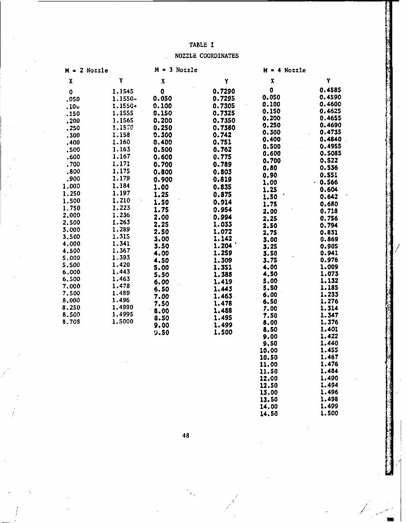
TABLE I

NOZZLE COORDINATES

M4 2 Nozzle M =3 Nozzle M 4 Nozzle

0 1.1545 0 0.7290 0 0.4585SI.050 1.1550- 0.050 0.7295 0.050 0.4590

. oo1.1550+ 0.100 0.7305 0.100 0.4600.150 1.1555 0.150 0.732S 0.150 0.462S.200 1.1S65 0.200 0.7350 0.200 0.4655.250 1.1570 0.250 0.7380 0.250 0.4690

.300 1.158 0.300 0.742 030043.40 1.60 .40 0.510.400 0.4840

.500 1.163 0.400 0.762050 .45

.600 1.167 0.600 0.77S 0.600 0.5085

.700 1.171 0.700 0.789 0.70 0.522

.800 1.175 0.800 0.803 0.80 0.536

.900 1.179 0.900 0.819 1090 0.5511.000 1.184 1.00 0.83S 1.00 0.6641.250 1.197 1.25 0.875 1.25 0.6421.500 1.210 1.50 0.914 1.50 0.6421.750 1.223 175094.50601.SO942.00 0.718

2.0 126 2.00 0.994 2.25 0.7562.500 1.263 2.25 1.033 2.50 0.794

3.0 129 2.0 1.072 2.75 0.8313.500 1.315 3.00 1.142 3.00 0.8694.000 1.341 3.50 1.204 3.2S 0.905 S4.500 1.367 4.00 1.259 3.50 0.9415.000 1.393 4.50 1.309 3.75 0.9765.500 1.420 5.00 1.351 4.00 1.0096.000 1.443 5.50 1.388 4.50 1.073

7.000 1.478 6.00 1.419 5.00 1.1327.500 1.478 6.50O 1.443 5.50 1.1858.000 1.49 7.00 1.463 6.00 1.2768.050 1.4990 7.50 1.478 6.501278.500 1.4995 8.00 1.488 7.00 1.3148.708 1.14000 8.50 1.495 7.50 1.*347

8.0 .00 9.00 1.499 8.00 1.3769.50 1.500 8.5 1.401

9.00 1.4229.50 1.44010.00 1.45510.50 1.46711.00 1.47611.50 1.48412.00 1.49012.50 1.49413.00 1.49613.5 1.49814.00 1.49914.5 1.500

48

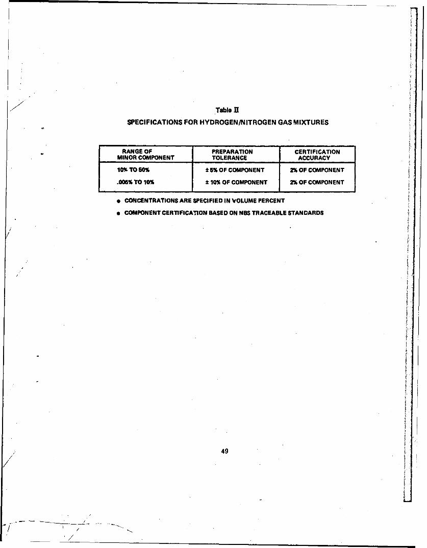
Table RI

SPECIFICATIONS FOR HYDROGEN/NITROGEN GAS MIXTURES

RANGE OF PREPARATION CERTIFICATION

MINOR COMPONENT TOLERANCE ACCURACY

10% TO 50% 1 5% OF COMPONENT 2% OF COMPONENT

.006% TO 10% t 10% OF COMPONENT 2% OF COMPONENT

" CONCENTRATIONS ARE SPECIFIED IN VOLUME PERCENT

" COMPONENT CERTIFICATION BASED ON NBS TRACEABLE STANDARDS

/

S/

-I - -

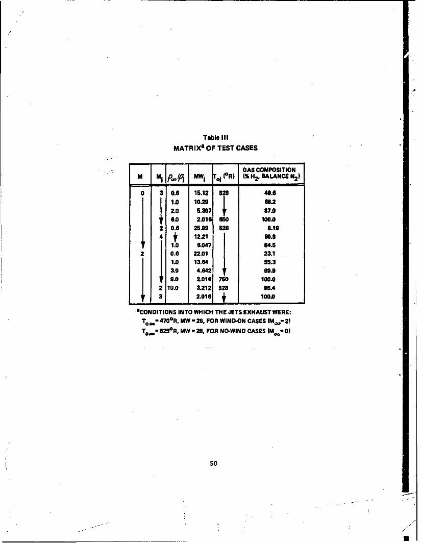
Table III

MATRIXa OF TEST CASES

GAS COMPOSITIONM M, pm MW ro (OR) 1% H2.BALANCE N2 )

0 3 0.6 15.12 528 49.61.0 1029 68.22.0 6.307 87.0

6.02 2.01650 100.02 0.6 25.89 528 8.1941 12.21 60.8

1.0 6.047 84.2 0.6 22.01 23.1

1.0 13.64 55.33.0 4.642 89.99.0 2.016 750 100.0

2 10.0 3.212 528 96.4

1 3 2.016 1 100.0

aCONDITIONS INTO WHICH THE JETS EXHAUST WERE:

To., 470°R, MW - 28, FOR WIND-ON CASES (M,,- 2)Too" 5230 R, MW - 28, FOR NO-WIND CASES (M"- 0)

s0

* 7

o- - U

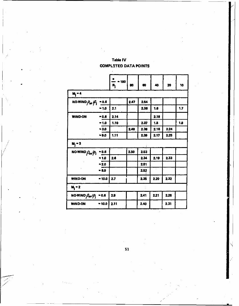
Table IV

COMPLETED DATA POINTS

xlS,100Ri s0 6 ) 40 20 10

i ---

NOWINDOgafj -_.6 2.47 2.54

"1.0 2.1 2.36 1.6 1.7

WIND-ON -0.6 2.14 2.18

1.0 1.10 2.37 1.5 1.8

"3.0 2.48 2.38 2.16 2.24

"9.0 1.11 2.3 2.17 2.25

NO.WINDp -0.6 20 2 3

"1.0 2.6 2.34 2.19 2.33

"2.0 2.5i

M6.0 2.52

WIND-ON -10.0 2.7 1 2.35 2.20 2.32

MI-2

NO.WINDp.(j -0.6 2.9 2.41 2.21 2.28

WIND-ON -10.0 2.11 2.40 2.31

51

7 s

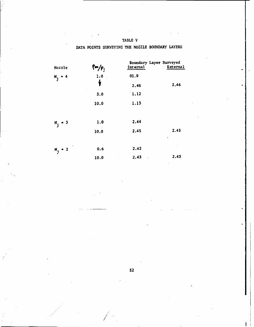
TABLE V

DATA POINTS SURVEYING THE NOZZLE BOUNDARY LAYERS

Boundary Layer SurveyedNozzle "/.Internal External

M4. =4 1.0 01.9

2.46 2.46

3.0 1.12

10.0 1.13

Md. =3 1.0 2.44i

10.0 2.45 2.45

M. 2 0.6 2.42.1

10.0 2.43 2.43

52

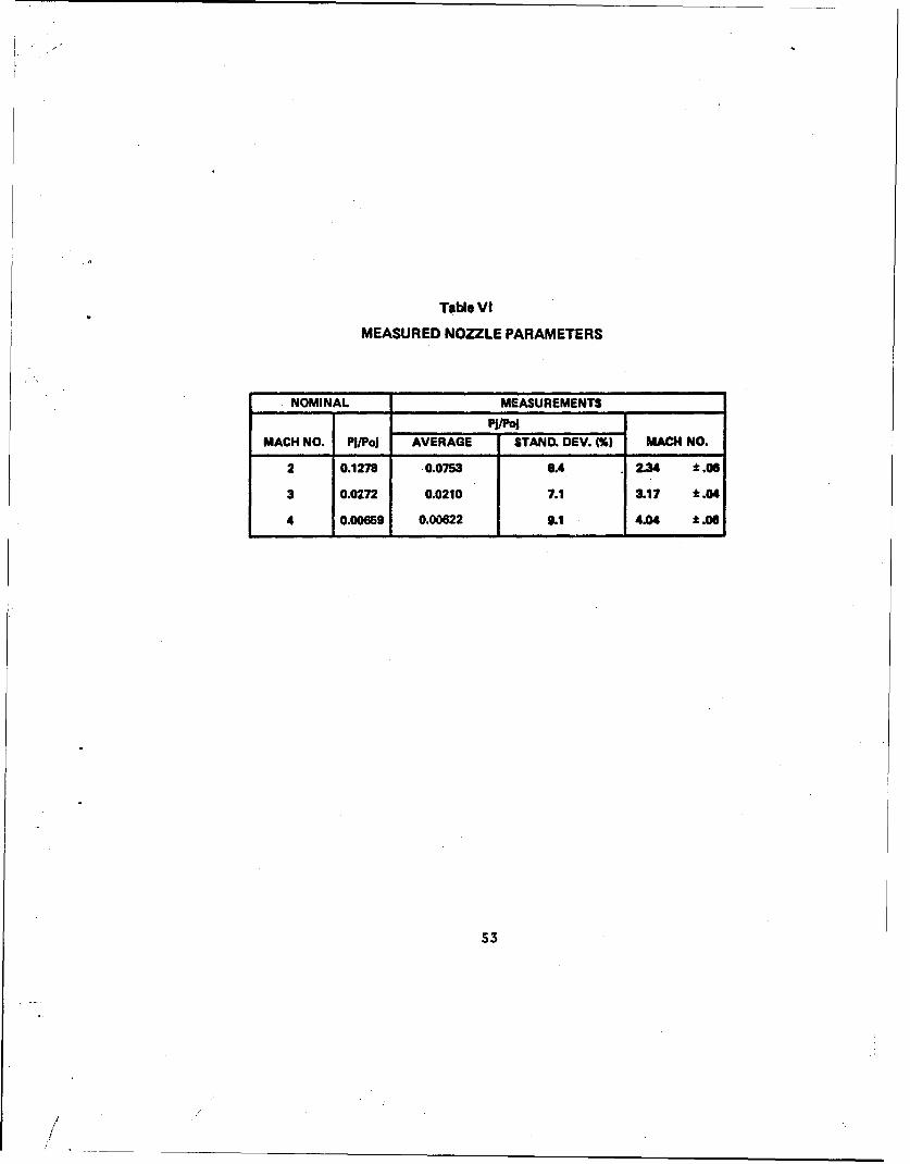
Table Vt

MEASURED NOZZLE PARAMETERS

NOMINAL MEASUREMENTS

MACH NO. Pu/pal AVERAGE STAND. DEV. (%) MACH NO.

2 0.1278 .00753 8.4 2.34 ±.06

3 0.0272 0.0210 7.1 3.17 t .04

4 10.006691 0.00622 9.1 14.04 ± .061

53

(4 -7 qtr '0%' s O 0 N N -4 00 GO M~cc N-~00 ON cc0"' N -4 M 0 N N LA .-4 0 0 -'- 0 -4 cc a cc %0 W' ' . Ln N N N 0 -4 -4

cc 1=' 00 N N0 00 O m 00 -0 010 00 -IO '0al0I % O l 0 C 0

- ON N -C! 0 N: e '":No c 0n M -4 C D '.0 P-4 V" o0 r-4' cV) a. 1.N-4 t1 .o -4 N c

0u N -00 (4 N 0 N0- N -00 w 0-sr. " -b - r- - (1 -4 r- w " - - - N t-

00 00t LA r- mJ 00 LA r, L) C r4 m' 0A t4 m V 4 m 0

X Z ON .0w CD m (M t 0 N -0V0 -4 Go Nn 0 0 r- %A 0 %0cc0tA 4 N a ' "0 0 0 -4 N a C4 rA - q c 0 - 0 '0 Cc~~. .- 0 N N O 0 0- 0 0. . . . . - . o N 0 0.

LL. %

N- tl z. m Nq cc N"

CL C3. ND %. N - v -0 00 -0 to) 0n 'T 00 c N0 LA V) LA N LAW C I A C 14 C 4 A t ~ L O N - "4 ("' 0 A - qC 4 0 4 0

cN LA Z. (N C% - N LA - cc cc M A N n LA %0 cc LA '4 N LAw 0~ C4 0) t) mA N LA W), " N1 N N1 N1 to) 14 N 4 "i N - -4 0u - 0 tf'. LA mA LA LA NI LA LA LA LA LA LA LA Nf LA LA LA LA Ul Nl L LAz

LW

u. ON CD0 0 N LA '0c N0C' tAn t '.0 M LA 'O00c N %0~ N- - - - 00 cc 00c - - -q cc -4 cc V -- cc

N c N 0 '.0 0 0 Nq 0 cc '0 0 ccx

cc LA LA 00 w LA N N -T -4 - N1 NcisNN -c T cc '0 Q'TT00 ' 00 ON m c ON M 00 0cc( 00 04

zA - o c (1 NC 00 00 '0 N a '0'0 '0 . c 00 ~40 0

C44 .4 'LA An '00 ,T LA C, NO N ,1- '0 N c c 0 0 N 0 '0 LA '0

(D "' -n -4 -n - 'D -r <n t,- r- -4- - -D -D -n z

-4 -4 1. "z .n 0

0~ ~ M4 -' C' M. c o 0- A c

54

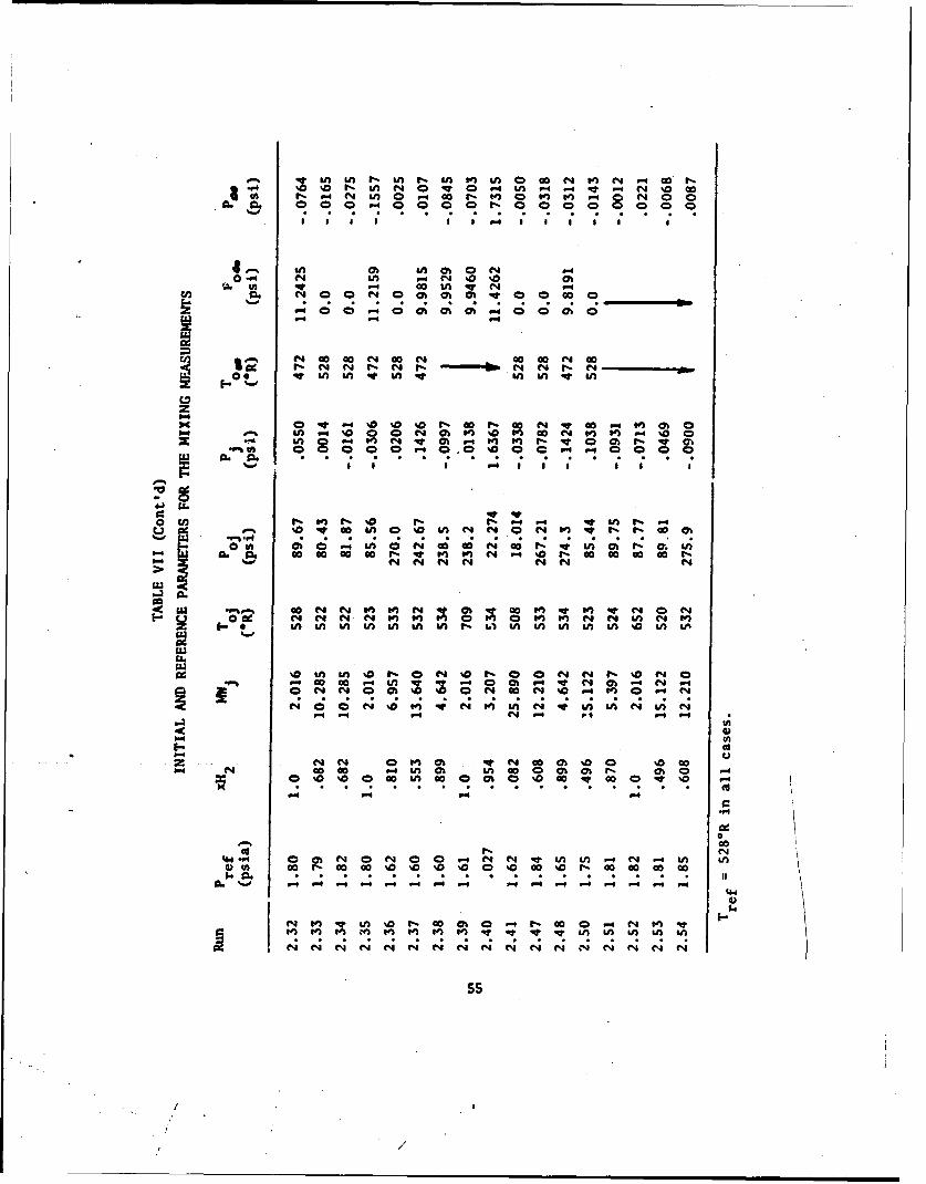
a.- In r n f. In m' in 0.0 Go M N -. 00 It.%a [- a. N O ( 0 . n a V4w r4 -.4 -4 " %0.w

f-. 00 In 0 f- W)~ 0 In 101 - N a0

0 4 04 LI I4 %0 %0 a a a

ta V

c4 C-40

1% N N -N -'- - Nm N4 C4 NvU I in) v %n v In In v I

z-4 C

0 cn Il n O % I'D r% V~ - ) 1) ln~0 1.% P-

: a o -v ao an c ao i 4 t - t ao a.

90

00 0 C n ' mn NN ON A ) "t C4 a- Na0~ W ~ C 0 In ON "0 N0 m a. " IN Ob "~ m~I

w~ A.A 0000 0 w .Ln I') I'n Nl w . L n4 w0a V%000

0N Nn N N- N 4% -a C N N4r-%

-JA

16.

-! .00 F.~ o . 00. NV.-

NN 0O O CN.0 vN0 -40 -4NLNcO w N'09 %D No %0 "o N In In N In N" w

- P4 P4 N 4 P1;_ -4 -

i ll i l "t Li U li iIL

r4 C4 C 4 C 4 r 4 ' 4 % 4 C4 C

2 N 0 I) O ~ (U 000 '00 '00

TABLE VIII

INITIAL VELOCITIES AND ACTUAL DENSITY RATIOSFOR THE MIXING MEASUREMENTS

Run u. u,

(fps) (fps)

1.5 3400. 1614. 0.991.6 48A5. 0. 1.121.7 4849. 4 1.121.8 3400. 1614. 0.991.10 3390. 0.991.1 9940. 8.47

2.1 4854. 0. 1.12VP 2.6 3380. + 0.97

2.7 7605. 1614. 9.862.9 1776. 0. 0.602.11 5043. 1614. 9.762.14 2510. 0.602.16 5519.{ 2.922.17 9847. 9.302.18 2515. 4 0.612.19 3383. 0. 0.972.20 7656. 1614. 10.002.21 1754. 0. 0.59

2.24 5524. 1614. 2.932.25 9679. 4" 8.992.28 1737. 0. 0.582.31 5057. 1614. 9.812.32 7656. qP 10.002.33 3370. 0. 0.962.34 3370. 4' 0.962.35 7620. 1614. 9.902.36 4508. 0. 0.972.37 3216. 1614. 0.992.38 5524. j 2.932.39 9658. 8.952.40 S075. 9.882.41 1742. 0.0 0.532.47 3403. 4' 0.552.48 5524. 1614. 2.93

, 2.50 2782. 0.0 0.66~12.51 4662. j 1.84

2.52 8508. 6.13

2.53 2774. 0.652.54 3400. 0.55

I5

,z z

w

-- JItI32 j

zaj4

U

cr..

w

57

- w

ww2 0.

zx

CL

<U

00

0 w

IO

Ix >

58

LU 2

LLU

0 2.

i

LUJQI2 LU

CL ,

C', 0> U.

Z~ 200

2

U N<

NU 04zN 0-I

xz

4 LU

uuJ

U.

59

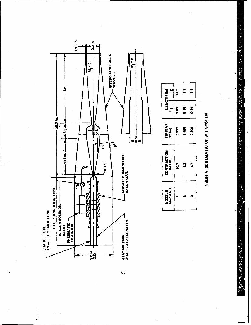
U-U

cc iN

I fq * *

a a.

r. ).

d- 90

0 v

-jt 0

U~w- 4

Wa~ >,SX

0 0

C!60

za/

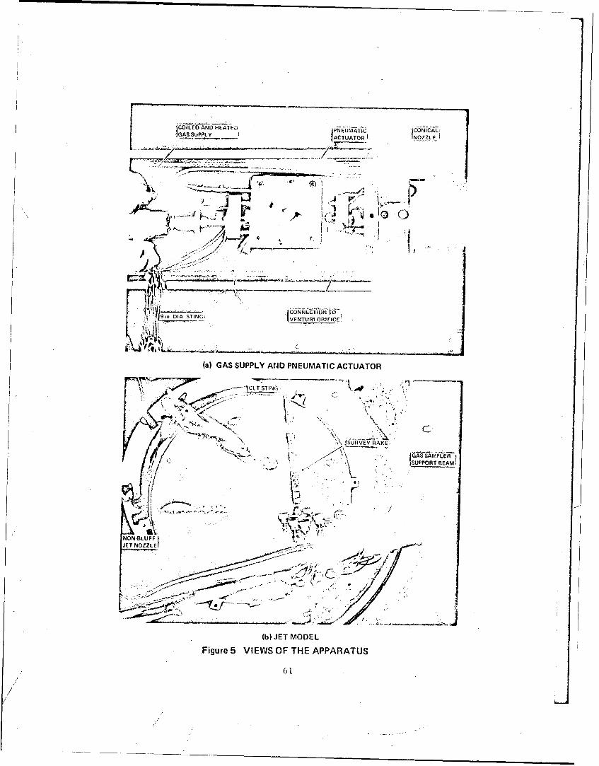
COILED AND HEATE -NEMAI- -NIA

ASSUPLYACTUATORII NOMZE

44-- I)'

9.n DIA STIN~iCO0N NECTIOUN TO7j ~ ~ ~INIVFNTURI OR IFICPL

(a) GAS SUPPLY AND PNEUMATIC ACTUATOR

-,-'CLT STINGi'

SU RVEY RAKE;

SUPPORT BEAM

NON BLUFFJET NOZZLE!

(b) JET MODEL

figure 5 VIEWS OF THE APPARATUS

6 1

C!"

NN N No a 0 0z z cc0

I-

01

P4

62

.

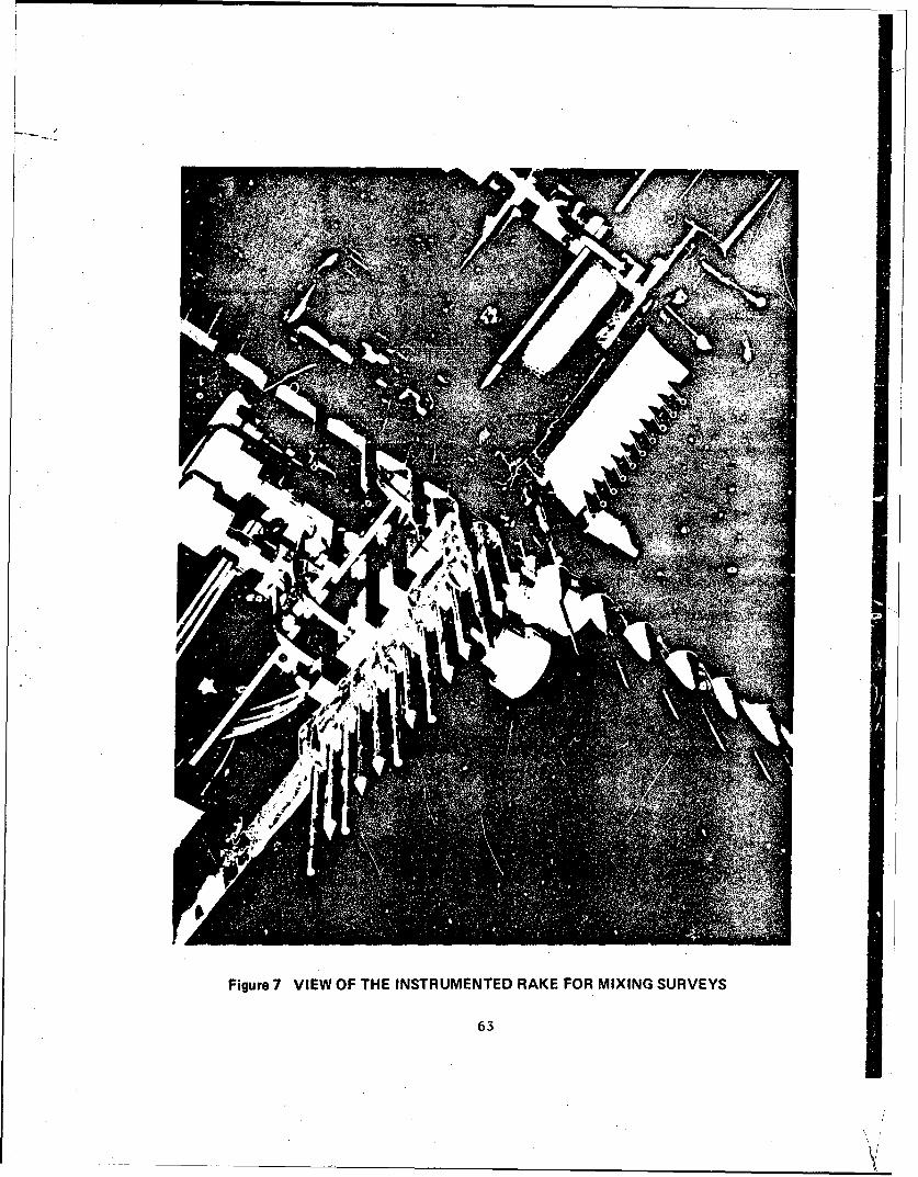
Figure 7 VIEW OF THE INSTRUMENTED RAKE FOR MIXING SURVEYS

63

0,.001 IN GAGE THERMOCOUPLE MOUNTED INSIDE THE VENTED TIP

TEMPERATURE PROBE

1 4anH

TRANSDUCER

FOUR 0.008 IN DIA. HOLES

Figure 8 VIEW OF THE PROBES FOR GASDYNAMIC MEASUREMENTS: (a) SINGLE PROBES

o4

CASE COVERING TRANSDUCERS*1< LOCATED 2.5 IN FROM PROBE TIPS

0.07 1 IN I.D. PROBES §i44

aan

0 20 inIDPROBES

Figure 8 (Cont.) VIEW OF THE PROBES FOR GASDYNAMIC MEASURESMENTS:(b) PITOT PRESSURE RAKES

(15

2 ~I~2

wU > 1-i- -

1- -' 19F.c0 wo- sLU C1 1

z i-. 40 f04

UJ cac -0 OL k -j

0i 0

LU 4 - ccCA -L

z 0

lW 0 x1 '

(A C0 > -0 c o u s. I =

cc 000

LT T1 1.

0l 2U- ..- 5 )'

L4 21- 4D> > L

0

2 2

<cc,

x

66

KE LEETSO TESTMSELACUTR YTE SE-EX4OR-.TIS

SKEY (b ELMNSSFMTHED TEM-SALETUTR OSYSTEMSTXTFRDALS

Figure 10 VIEW OF THE PROBES FOR GAS SAMPLING

67

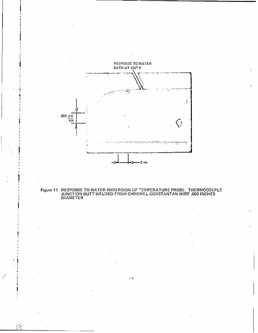
RESPONSE TO WATERBATH AT 1600 F

200 g'V

2 ms

Figure 11 RESPONSE TO WATER IMMERSION OF 'TMPERATURE PROBE. THERMOCOUPLEJUNCTION BUTT-WVELDED FROM CHROME L-CONSTANTAN WIRE .003 INCHESDIAMETER

RUN. 24 SERIES. 2

r0 lT i3lN EDYNAMIC PRESSURE: 7 PSIA

1201------------- GAS COMPOSITION: 55H

BALACE N2

w

AMBIENT -w- .0 T

-128--- - - - - - -~

-40. it It. 2. ISO. M3. 240.PROBE AT 2.5" FROM 4L

RU.24 SERIES.

121-DYNAMIC PREISSURIE -5Po GAS COMPOSITION: 100% N2

AMBIEN4T

-2011 1 1 , i-40. 6. 4. i0. 1n. Ise. 299. 246.TINE NILLISEC

PROBE AT 6" FROM (L

Figure 12 RESPONSE OF THE TEMPERATURE PROBES IN THE JETS AT VARIOUSCOMPOSITIONS AND LEVEL S OF DYNAMIC PRESSURE

69

RUlI. 52 SERIES" 2

12u

DYNAMIC PRESSURE -0.6 PSIA

AMBIENT AS COMPOSITION: 72% H2

-40. . 4. . 129. 161. 2". 24 .

TIME NILLISEC

PROBE AT 1.5" FROM %

RUN* 25 SERIES. 2

DYNAMIC PRESSURE - 30 PSIA

GAS COMPOSITION: 100% H2

0

LU°0

AMBIENT

4-0N

-46. 6. 40. 8. 120. 166. 296. 240.TIME HILLISECPROBE AT 0.5" FROM .

Figure 12 RESPONSE OF THE TEMPERATURE PROBES IN THE JETS AT VARIOUSCOMPOSITIONS AND LEVELS OF DYNAMIC PRESSURE (CONTINUED)

70

N Nt

Al U.

u IL

bOO04000* wj

o 20,

NW 2cc~ 00c

0<

o02

-jzI-.

IL

to V0 40N

AUTOVAC PIRANI GAUGE READING fmV)

71

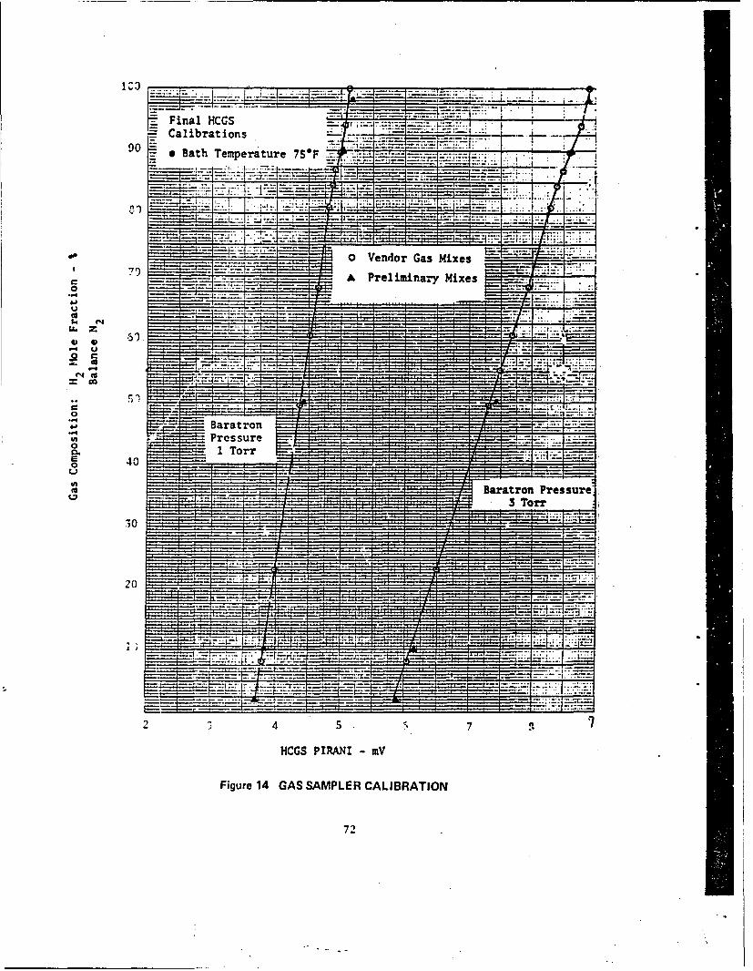
Calibrations

90 ~

-- FI

0

30

.0.

4 7S

HCGS PIRANI -mV

Figure 14 GAS SAMPLER CALIBRATION

72

ww

t w

ww

-0

ww-rr--- 0'L c I -

_i :-4AtT 1 _ __0

' pCC

)~'-~Lt'wU ( ~ .

w LU

z

4uc0 :LoC4A

+ ~ ww~

z w 0i

o

< - C6-- /U _- ILL

I- D CC

WL I Lo *Pz " --i- a

Z CL

LLCwu r-r.Z C

w j LL0.L

IcI0w

ccc'I v

V 0

a.'.

I-L

8 !ww

a.la

7449

............. . . .......

0

LL

Co. . . . .LLI1

CD 00DCA(w CD - .- a. ' - -. o s-n- . M - .M

~ WUJ~aJ WW~)U~(0C) C DCCOCCDCCN)DCMU)

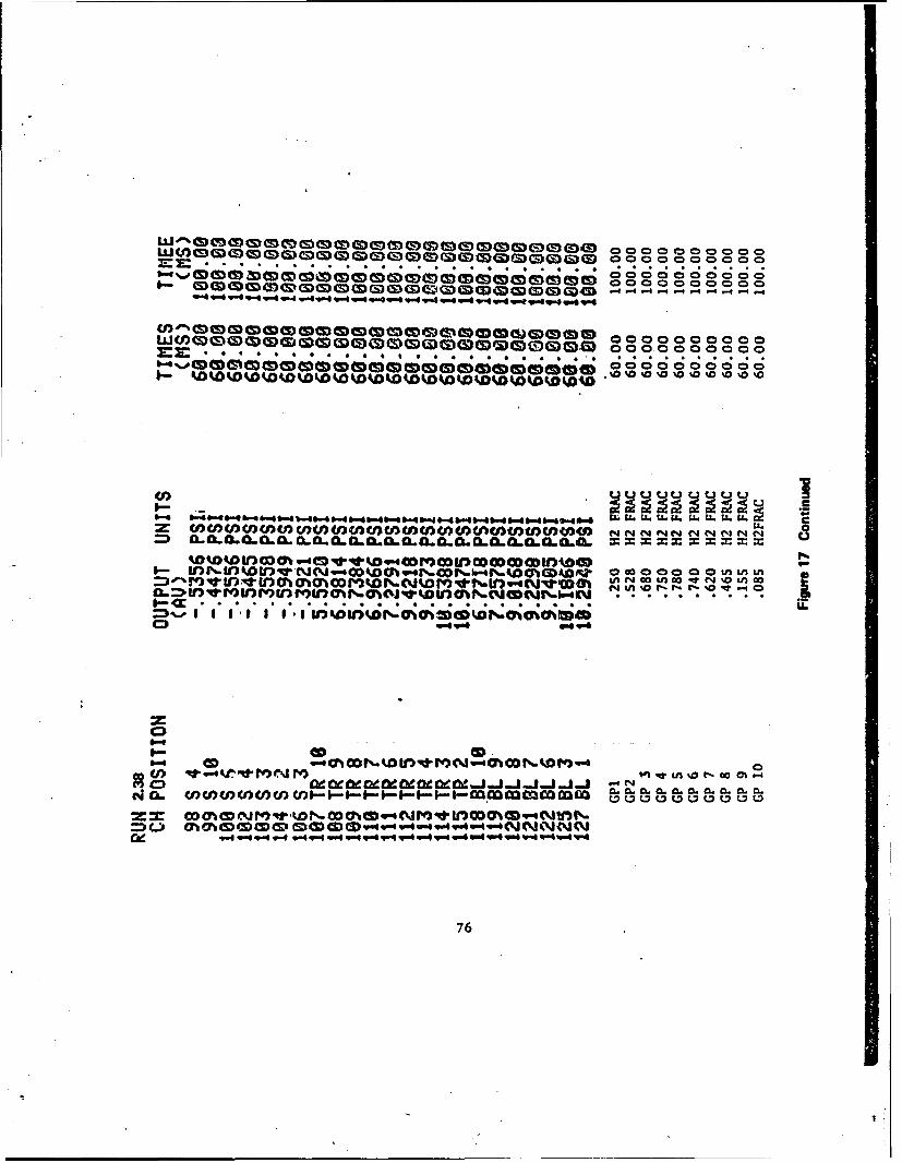
=E: . . .. . . . . . . . . . . . . .0 0 00 0

~4 ~4- q4~4 4 - -- -~4 w - - -4,4-4 41-4 -4--4-4 4--

0000

WWW 00 h W(m V",W- W000000000~olnf*4..V)W"V, ~ ~ ~ ~ ~ '0( V"CW0 o%(*(C4'k0W 0 ~O0 0 L0 '0

F- CCD0 ~ j 0aocottt

Aw ~ ~ .* .- 4p .d M ". " .0 .n . *CD I II I www ww~wNJ--UJ-- MG 0.. " . . .

0 o~o icnhDW-V O

760

WIND-ON -

ZS Pct oa. A -k -"- -

V .I I-

A2 - - -I-

mat.

sTo

20 m/div20s/i

DOIN

-S-

rri

Figure 18 HISTORIES OF FLOW VARIABLES ILLUSTRATING THE JET/STREAMCHARACTERISTICS

77

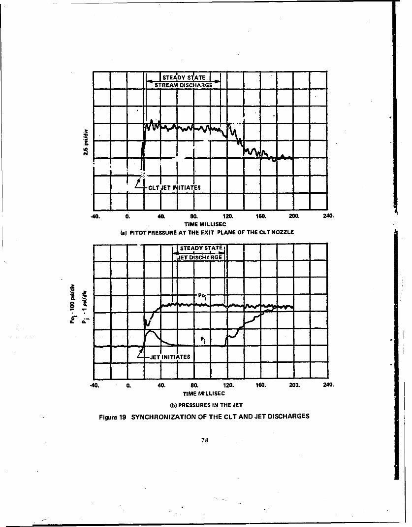
STEADY STATESTREAM DISCHAIGE

mf

sq%

No

-CLTJET INITIATES

40. 0. 40. 80. 120. 160. 200. 240.

TIME MILUSEC(a) PITOT PRESSURE AT THE EXIT PLANE OF THE CLT NOZZLE

t STEADY STATE

I lJET DISCHtRGE

aPol

I P6

AJETINITIATES

-40. 0. 40. 80. 120. 160. 200. 240.

TIME MILLISEC

(b) PRESSURES IN THE JET

Figure 19 SYNCHRONIZATION OF THE CLT AND JET DISCHARGES

78

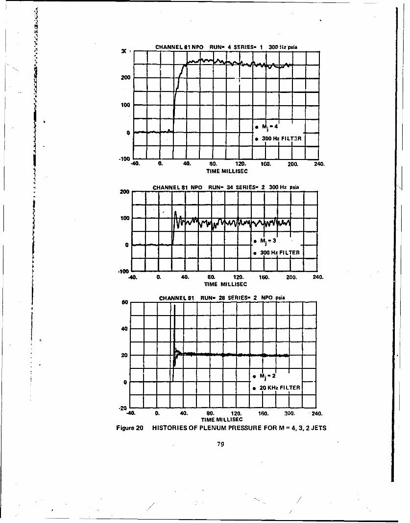
II

CHANNEL 81 NPO RUN- 34 SERIES- 1 300 Hiz psia

200 -- A - -

0~ M-3

.100-~~~~~ CHNE 1NORN 300HzFILTER

-40. 0. 40. 80. 120. 100. 200. 240.TIME MILLISEC

I - -CHANNEL81 RUN- 28 SERIES- 2 NPO psia

20--

M M1 2

20 2KHz FILTER

-40. 0. 40. 80. 120. 160. 200. 240.TIME MILLISEC

Figure 20 HISTORIES OF PLENUM PRESSURE FOR M= 4, 3. 2 JETS

79

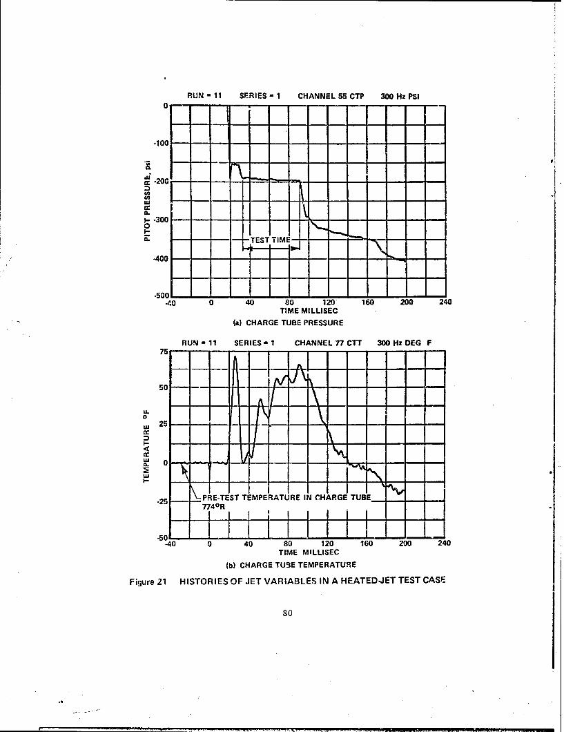
RUN =11 SERIES 1 CHANNEL 55 CTP 300 Hz PSI

a. 20

0

0. --- -TEST TIM- - -

-40 0 40 80 120 160 200 240TIME MILLISEC

(a) CHARGE TUBE PRESSURE

RUN-l1 SERIES-i CHANNEL 77 CTT 300 Hz DEG F

50 - -- "

0

a. 0 - -

-25 PRE-TEST TEMPERATURE IN CHARGE TUBE_ _

.40 0 40 80 120 160 200 240TIME MILLISEC

(b) CHARGE TUBE TEMPERATURE

Figure 21 HISTORIES OF JET VARIABLES IN A HEATED-JET TEST CASE

80

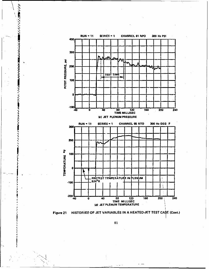
RUN " 11 SERIES 1 CHANNEL 81 NPO 300 Hz PSI

: 400

CA

w TESTTIr E---------------a.100

0

I-

--

100-

T-40 0 40 P 120 160 200 240TIME MILLISEC

(c) JET PLENUM PRESSURE

RUN- 11 SERIES I CHANNEL 65 PJTO 300 Hz DEG F300

i200 F

W

I IImPRETEST TEMPERATUR IN PLENM

- -o 524°R"

--200 E-40 0 40 s0 120 160 200\ 240

TIME MILLISEC(d) JET PLENUM TEMPERATURE

Figure 21 HISTORIES OF JET VARIABLES IN A HEATED-JET TEST CA E (Cont.)

81

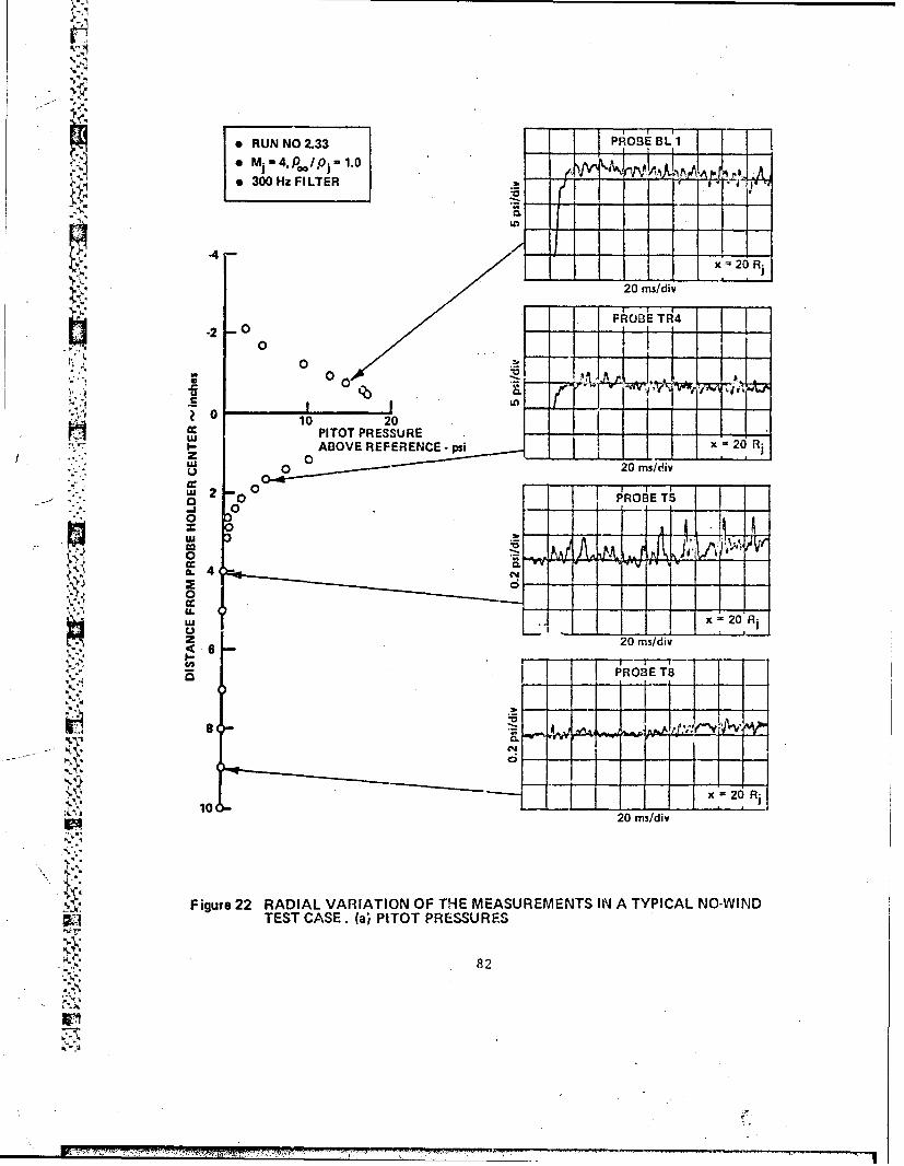
. RUN NO 2.33 PROBEi BL1 JI

-42 xms/d iv

-*- M.4PI .

:.:, .SUI I_

4- PITOTIPRESSURE

20 ms/div

- --- PROBE T14

0 10 20

0 20 ms/div

" -' i ! ' 'L0.PRSSUR PROE--a 00x 0i

0 &w v, I

a. 4 04.-

0 2U _ .

,)"- - " -' x =20 Rj

2 20 ms/div

PR03E TS

2ms/div =0R

Figure 22 RADIAL VARIATION OF THE MEASUREMENTS IN A TYPICAL NO-WINDP. TEST CASE. (a) PITOT PRESSURES

82

+I,

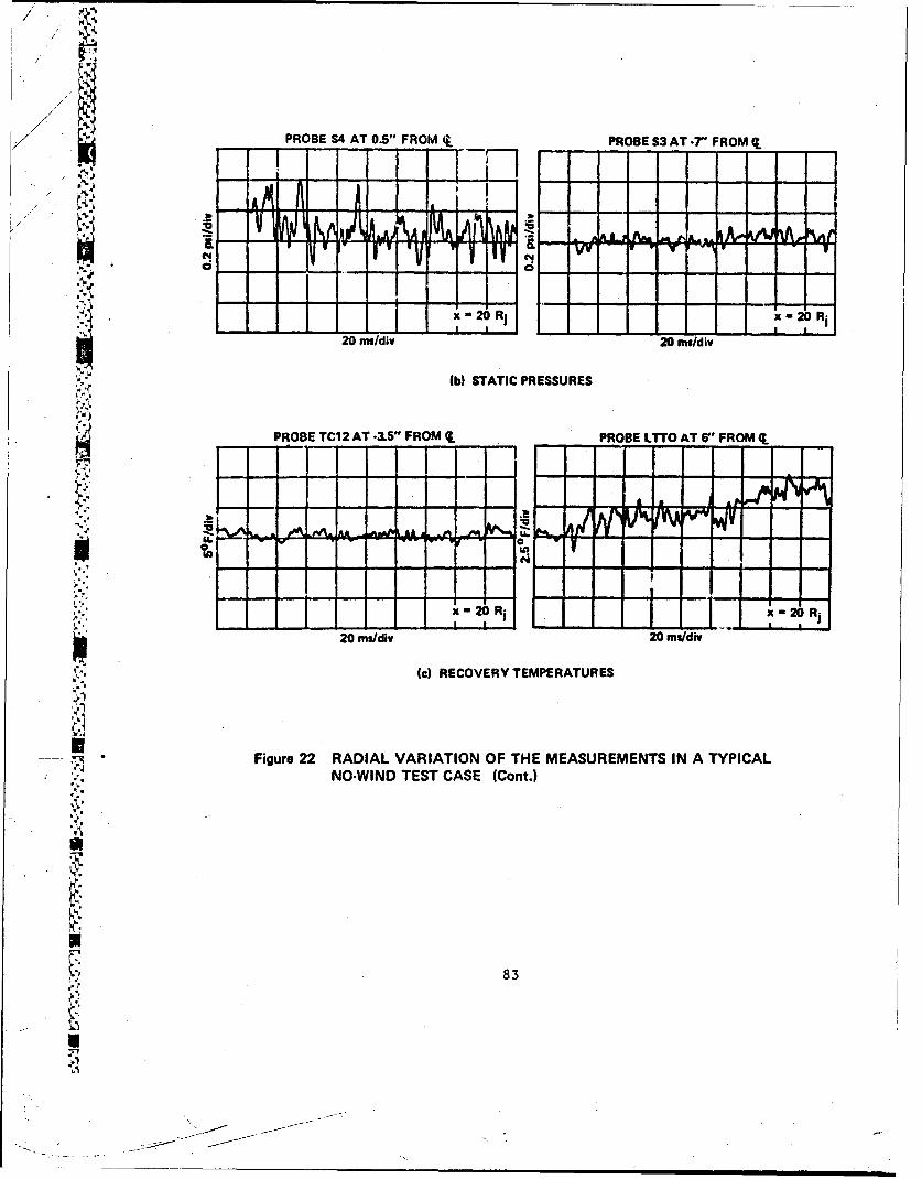
PROBE S4 AT 0.5" FROM _(L PROBE S3 AT -7' FROM

VZ ' r -. "JAL-- ~-

- - -. - - -~~ - - - - - - -

-- ~2 Ri20R

(b) STATIC PRESSURES

PROBE TC12 AT -3.5" FROM (L PROBE LTTO AT 6"* FROM 4-

A&..- 40d 03-f Sn

JII20 X02RR20 ms/div20m/i

(c) RECOVERY TEMPERATURES

Figure 22 RADIAL VARIATION OF THE MEASUREMENTS IN A TYPICALNO-WIND TEST CASE (Cont.)

83

* RUN NO Z6

1 .4

0

I w E 100R.2I PITOT PRESSURE

'U 0 04 0.8 ABOVE REFERENCE -pu Ou/i

'U PROBE T5

O 0

02 0 d.---

Iz 20 mAd

au50 20msdi

6 - 0 - - -

x100CR17 L 20 ms/diw

:4 Figure 22 RADIAL VARIATION OF THE MEASUREMENTS IN A TYPICAL NO-WINDTEST CASE 1d) PITOT PRESSURES (Cont.)

84

PROBE S2 AT 1S FROM q

1------------------

=/mndiv

PROBE S3 AT 7- FROM q.

x 10 Ri

20 nis/div

Figure 22 RADIAL VARIATION OF THE MEASUREMENTS IN A TYPICAL NO-WINDTEST CASE (e) STATIC PRESSURE (Cont.)

85

.;/" !

.I

a RUN NO. 2.24a M- 4. 0 0 /P -3 PROBE BL 9

o 2CO Hz FILTER- i -

Ii

-4

.J.

x-20 Re

.2 O 20 ms/div

0 PROBE BL 6

, 10 20 10 L- ad -o,, ,U PITOT PRESSURE . p I 'oo"1-r;r' u~~l" ABOVE REFERENCE - psi 0 -

00nI

w" 2 0-O-0 : x -20 Rj

0 0.w 0 20 rm/divLu

004. 0

wcj:

'<U 6 PROBE T8

0 "-

0- NIn.I

x: '20 Ri'* 10 - - -- j 2fl

20 ms/div

SFigure 23 RADIAL VARIATION OF THE MEASUREMENTS IN A TYPICAL WIND-ONTEST CASE (a) PITOT PRESSURES

t,8

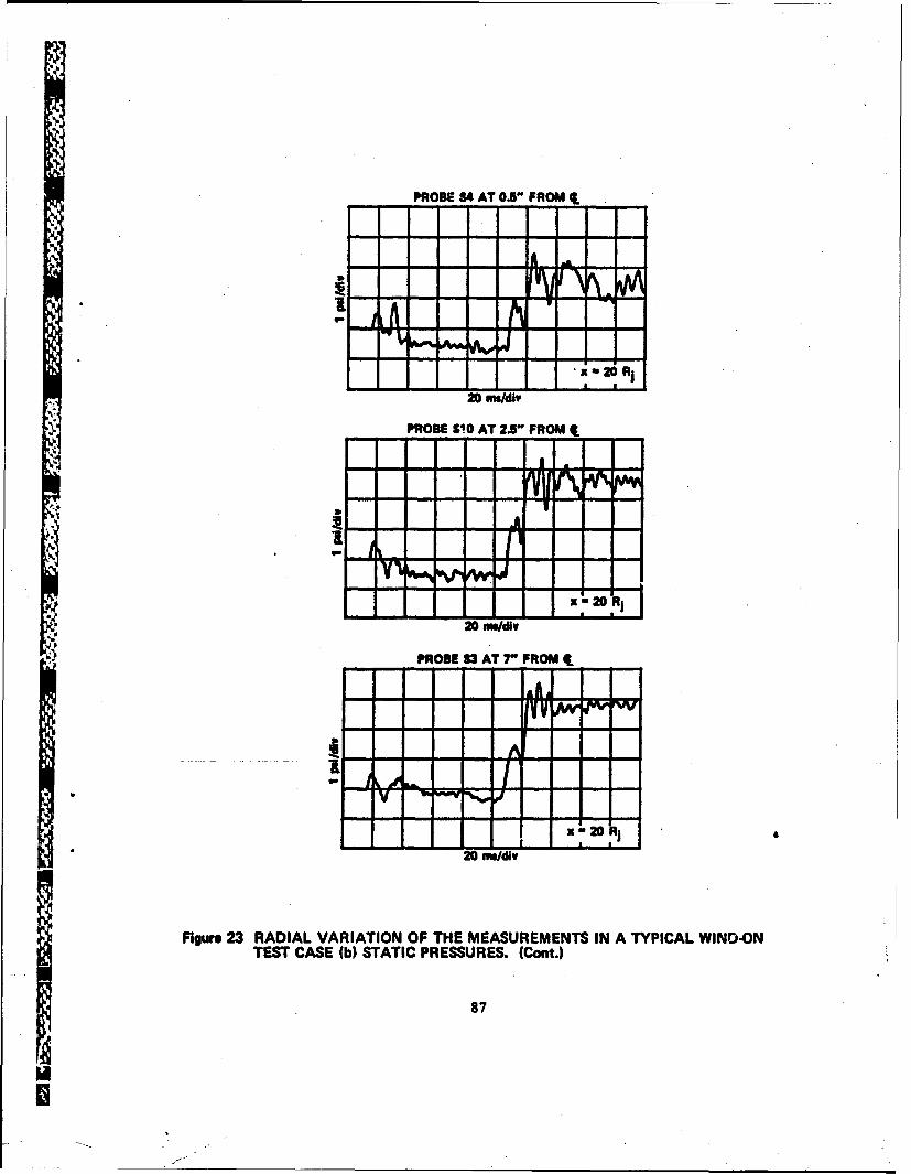
PROBE S4 AT 03- FROM

I- -/ -ILI

X" 20 Rj! I

20 ms/div

PROBE 510 AT 2.5" FROM t

x'.20 jIL

x 20 R

20 m/div

PROSE 313 AT 7" FROM .

20 maldiv

Figure 23 RADIAL VARIATION OF THE MEASUREMENTS IN A TYPICAL WIND-ONTEST CASE (b) STATIC PRESSURES. (Cont.)

87

PROBE TC13 AT 0.5" FROM It

x a 20

20 ms/div

PROBE TCl I AT 2.5" FROM 4L

PROBE TC12 AT 6" FROM q

x -20 R

20 im/div

Figure 23 RADIAL VARIATION OF THE MEASUREMENTS IN A TYPICAL WIND-ONTEST CASE (c) RECOVERY TEMPERATURES. (Cont.)

88

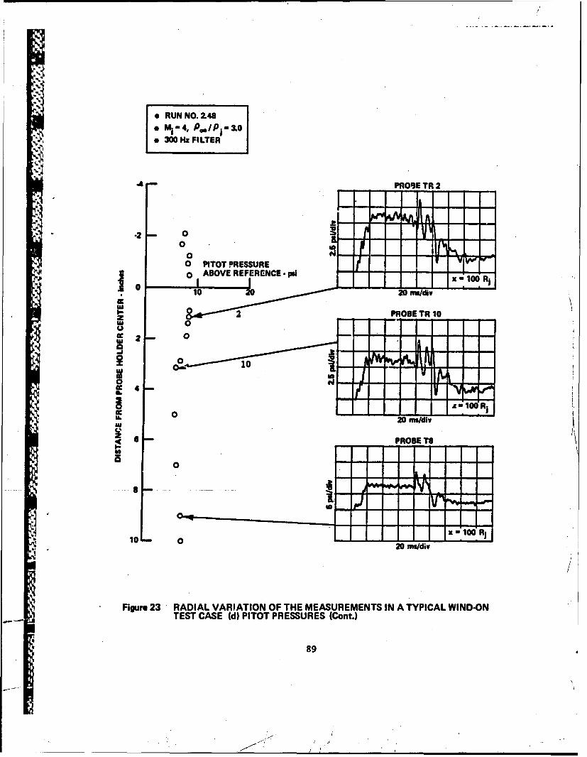
s RUN NO.2.48o M 1-4. P,,IP 1 &o

. 300 Hz FILTER

4 PROSE TR 2

0 1

OO P4TOT PRESSURELIIoABOVE REFERENCE -psi - 10- --

j0 - - - I 20 Isav- '

22 PROSE TR 10zLU0

0 . .

U.020'odU

PROE T

0

10- 0 2 sdv x10

Figure 23 RADIAL VARIATION OF THE MEASUREMENTS IN A TYPICAL WIND-ON- - TEST CASE (d) PITOT PRESSURES (Cant.)

89

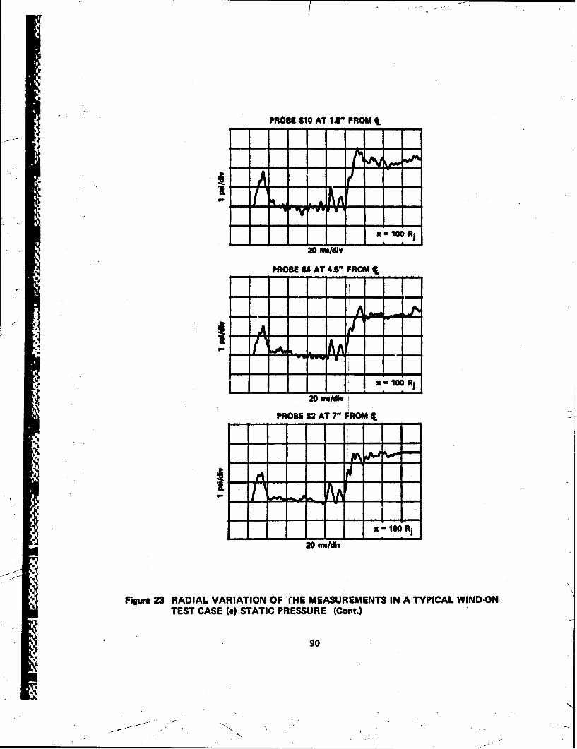
PROBE 810 AT 1A" FROM q

I100

20m/duv

PROBE S4 AT 43" FROM IL

a'. 100 Rj

20 fs/,iv

PROBE 82 AT 7" FROM 4L

106 100

20 m/div

Figure 23 RADIAL VARIATION OF 'HE MEASUREMENTS IN A TYPICAL WIND-ONTEST CASE (e) STATIC PRESSURE (Cont.)

90

• _ .

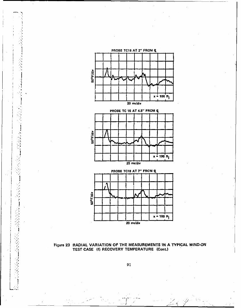
PROBE TC16 AT 2" FROM (L

iiiA -

jx100OO~i

20 ms/div

PROBE TC 15 AT 4.5' FROM (L

W)

-s R

1L116

10 R20 - -di

Fiue2 AILVRATO FTEMAUEETSI YIA IDO

TETCS ()RCVRYTMEAUR Cn.

PRBET1A7"FM

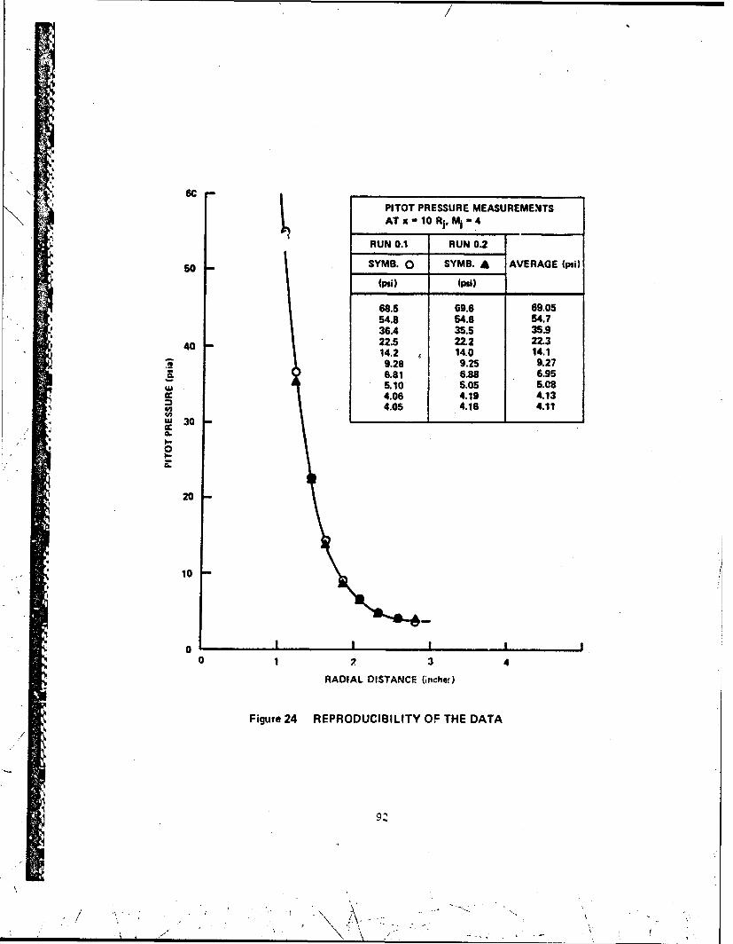
PITOT PRESSURE MEASUREMEN4TSAT x - 10 RI, M1I - 4

RUN 0.1 RUN 0.2

50SYMB. 0 SYMB. A AVERAGE fpsi)

fps!) (psi)

68.5 69.6 69.0554.8 54.6 54.7

*36.4 35.5 35.940 22.5 22Z2 22.3

14.2 14.0 14.1-49.28 9.25 9.27FL6.81 6.88 6.95

w 5.10 5.05 5.084.06 4.19 4.134.05 4.16 4.11

lW 30

20

* 10

0 16 1 10 12 3 4

RADIAL DISTANCE (inchef)

Figure 24 REPRODUCIBILITY OF THE DATA

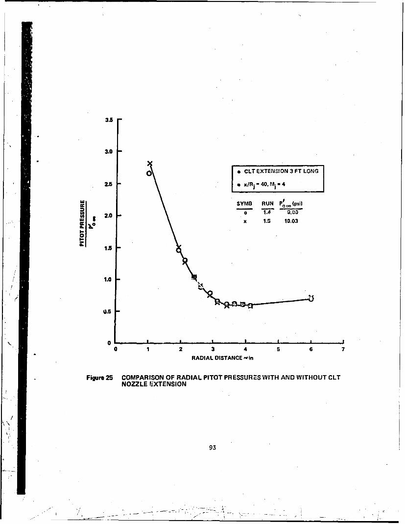
3.5

3.0

2 .CLT EXTENSION 3 FT LONG2.5[ o x/Rj" 40, rM l - 4

SYMB RUN P:,,,, (psi)

2.0 a 1.4 9.0x 1.5 10.03

C-" 1.5 -

1.0

0.5

0 1 2 3 4 5 6 7

RADIAL DISTANCE -,in

Figure 25 COMPARISON OF RADIAL PITOT PRESSURES WITH AND WITHOUT CLTNOZZLE F:XTENSION

93

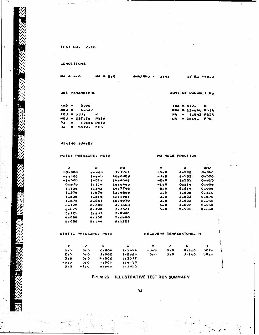
1&TNU. 9.10

04J 0 . MA as R. MA/fRNJ 4.v Af RJ -40.0

jkl PA.4AMCTt.4b AMblemr ~AmETems

X"'2 00%0v0 TOA a 47do a14W * ".*2POA mL 1389a PAA

1oj a 64.3. P4 P~A - 1.W43 PSIApoi3 & 237.76 PbotA UA a 3b54o FPSPj IL 5e5.o PSIA

VU.. a 661'I. FPS

MIARNG SUI4VEV

O'ITUC P.4ESSOIEs WjlA Pla UL#E F.4ALTIL)N

L e4 ..b0v 94 Ml-3.000 ad.934 7. 1;101 -5.0 4.002 0.060

-o 00 ~ 5060609 -3.0 2*503 00510-1.000 1.ood IW04*41 -200 1050b 00015

ob 1.11. lo0*o46 -100 0051f 0.vb01 . ldt I6.14i 1447745 0.0 0.51. 0OV063.J7* 1.676 1d.V306 5.0 1.605 0tosu1OI 5.0dt keel* 55.1a'Io Ide0 id.503 0.670I.1 obb i.051 10*497V 3.0 3060il 0. ie*02 0 .db it&300 i.Laftj 4.04 #6.b6 0 .0to

d 2o7V0 701611 to.0 5.601 0.080

3*1 dt 3.20*3 7.090040000 .4.*150 7.-d9o05 6000 6.5410 b o*

bTATIL PHbitvekE t~51 Otb.~V~4 1E^A~e.I

1** 0.0 e. 00. lslob' -0.6 0.0 0.1d0 :3i?.26 3.0 .3.002 1*2ddb 0.0 3.0 J.100 b02.3.5 0.0 4.o002 1.3617

-!3 a 0.0 -2001 1 .'! 100.0 -7.0 0.8o bSvb

Figure 26 ILLUSTRATIVE TEST RUN SUMMARY

94

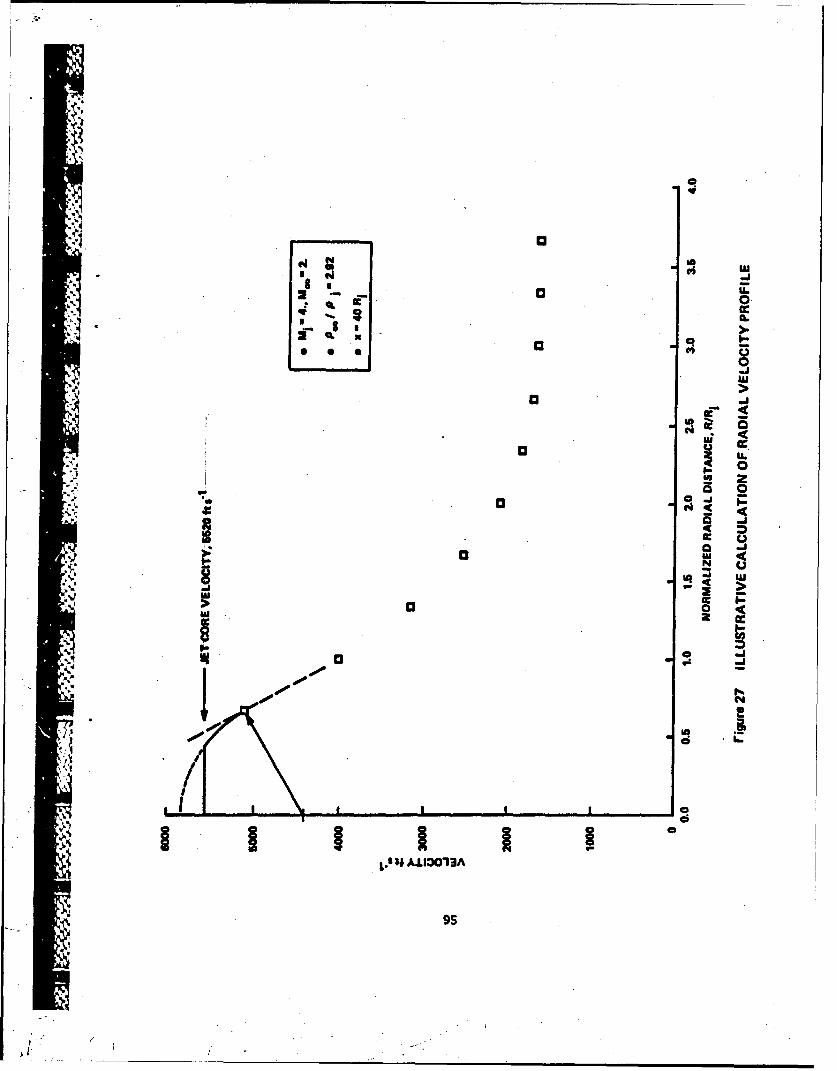
C

3m3

0>

0

0 -I

m0

IC! 2

4 9300

-j CI(

L-034ALI00.J

2 ~ C.,

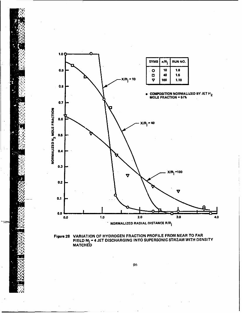
'A

1.0

'.,'* SYMB x/R RUN NO.

0.9 O 10 1.8X/R 10 a 40 1.5

V 100 1.10

" COMPOSITION NORMALIZED By JET H2MOLE FRACTION - 6i%

0.7',w'a

X0.6X/R 040

0~0.5

N0.4

z0.3

XR 0 100

0.2

0.1

V

0.0 n0.0 1.0 2.0 3.0 4.0

NORMALIZED RADIAL DISTANCE R/R.

Figure 28 VARIATION OF HYDROGEN FRACTION PROFILE FROM NEAR TO FARFIELD Mj - 4JET DISCHARGING INTO SUPERSONIC STREAM WITH DENSITYMATCHED

96

1.0 0

SYMBI x/Rj RUN NO

0.9 0o 10 12a0 40 isI

X/R1 10 V 100 J110110.8

*PRESSURE NORMAI.IZED BYJET PITOT PRESSURE 39 puia

0.7

cc~0.6

La

0.5

cc 0.4

0.1

0.0 II0.0 1.0 2.0 3.0 4.0 5.0

NORMALIZED RADIAL DISTANCE R/Rj

Figure 29 VARIATION OF PITOT PRESSURE FROM NEAR TO FAR FIELD Mj 4 JETDISCHARGING INTO THE SUPERSONIC STREAM WiTH DENSITY MATCHED

97

3500

X/R. 10

.LINES BASED ONBEST FIT THROUGH

W..XR 1 -40 DATA POINTS3000

el

'~2500

1500

10000.1 II0. .0 2.0 3.0 4.0 5.0

NORMALIZED RADIAL DISTANCE, R/R.

Figure 30 VELOCITY VARIATIONS FROM NEAR TO. FAR FIELD. Aj4.,Moo= 2, DENSITY MATCHED

98

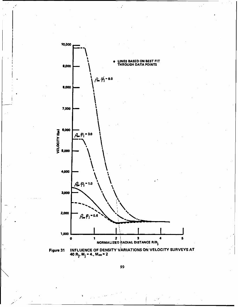
10,00

I . LINES BASED ON BEST FITTHROUGH DATA POINTS

7.00

4A00

2.00/0 - .

2.000

0 1 2 3 4 5NORMALIZED ADIAL DISTANCE R/Rj

Figure 31 INFLUENCE OF DENSITY VARIATIONS ON VELOCITY SURVEYS AT40 R.M 1 4., Mooin2

99

1.0 q -

o~s

0.6 SYMB 0pi

0 0 1.0l 0.4

V v 3.009.0

tU

' 0.2

bo

30 40 :0 60 70 80 90 100

AXIAL DISTANCE x/R

Figure 32 AXIAL DECAY OF JET CORE COMPOSITION

I

100

s/

IcCI

IU/'xHION3 3VI

10

200

1&.0

U12.0-

ifo 60

4.0-

0.0 p

0.80

- ~ 0.400

0.0

RADIAL DISTANCE (Incheui

1.;Figure 34 PITOT PRESSURE AND COMPOSITION IN THE MIXING JET AT x 20 Ri.- Mj 3JET DISCHARGING INTO STILL AMBIENT WITH DENSITY MATCHED

102

N

I--

Lu

Z

EICL)

0 0 LO

1030

APPENDIX I

MIXING MEASURE4ENTS

Test Case No. M M ?age

1 4 0 0.6 .1052 0 1.0 107

3 2 0.6 111

4I| 1.0 1135 3.0 1176 9.0 1217 3 0 0.6 12S8 I I 1.0 1279 2.0 131

10 6.0 13211 2 10.0 13312 2 0 0.6 13713 2 10.0 141

.4:

NOTE: For each Test Case, the measurements are presented byincreasing value of x/R..J

I

~104

./

/

. I' i '

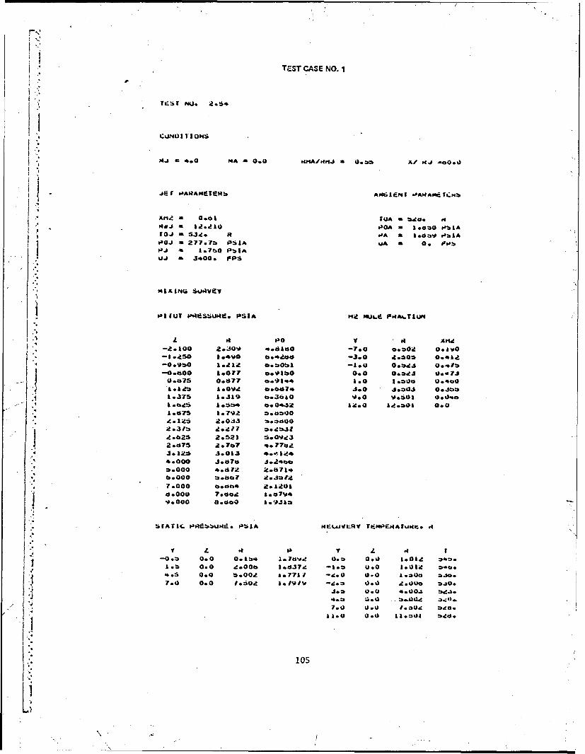
TEST CASE NO.1i

Ttdbf MU. 2.6,4

CU4O al A/ONS-0

xna 0.81 ro^ a two. .4p4wj a fl2.210 &30^ m 1.a0 l~l10.1 a 53g. R O~A a I.d 0 P'b1A

2JJ a277:7*0 PS:A U^ 0. Fobp~ a .7b0 PblAUJ a3*00 FPS

MLXANQ SUR4VEY

PI (UT PRESSURIk. PSI^ Pti AUJ&. Pv#Aii.TIUM

A it Po Y Vi

-2.100 2.30st '..dao -7.0 0.00id 0.1vO-1.450 1.490 0.4"d ~ -3.0 46606 0.41.1

-0.900 1.01? fteVobl 01.0 0.*ga 04?j 6.75 0.077 a9 %, 1.0 1 oun Q.A*boA t* A.0%0Z 0.07, ~ 3.0 .003 *.L*

1-375 1.319 0.36&0 .0 vosol 0.0-60

I .kg5 5.64 a0OJ3 &g.0 Ad.*04 0.01.075 1.7%02 0*00Q

2.3lt 2.417 gt?Z.625 2.521 5.40923

2.a75 a . V 4.77oz

7.000 8b.0"4 2.1201

d.000 7.o882 1.07vo

-A.000 a.doo 1.931*

SFAAIC PR4ESSURE PlbI HtiVLRY rtEMPEAFu#4kt it

-0.b 0.0 0:1b 1 rby 0:~ 0. 1:01Z *4I b 0.0 4.008 I 0372d -k b .0 1.012 ~a4.5 0.0 b.002 &.7?hl -,d.0 0.0 a .;a00 0o.7.0 0.0 1. "4 1.191so -,do 0.0 Z.000 340.

4.m 0.0 0.001 t2.3.

£1.0 1J. 1. o0 *do

K 105

TES(CCASE NO..

Vd.T We.g*

db. S.0 MA a 0.0 e~'ti a 0.ob A-f 14J sa0.0

id TPAAsQf .1S AFOdI A14Af0C idk

Ana a 0601 OA & 5400 It

Mai 1409.10 POA UI.o'.0 PbIATOJ - bi3. It PA A Isaga l~Abl

pj a 4.704 bbA

ui - .*0.30. frpb

MIXING SURvEV

'I 01~ D&Ebld *'OI "a M06k FMA..rIUM

-2o0 2daz 3.7446. --b.0 4.304 0.3W-1.700 1 o*add 3.b4b7 -.5.0 de#2 0..37

-1edo 1.461 40 %pip2 -100 0*407 ooav*0.9 ~ 1 I. dt0 4600a'0 0.00 004 .

-11500 Osa? *Iit 1. 04 03GU.aft 1*020 3.%p'd0 4d.0 oi 0.3

a 0b A 4 .5 300d -boo .041 0.G

1.0b 1o0. Jeboo0. 000460 U..e 0

Sd. oS4 1.w' .40b

dc~e* 4d*77 .J~V073.320 30121. J*__________________________

*.Vis .10

40000 161056 'doookf

STAT14. PRb'0bJegs PSLA I~.VI1Tu~ifM.5

4.0 .0 b140 .6OI? U.0 t.o.44 0b

0. .h4 1.w7 4 0. -to 0.601 _ b4d.1.0 000 d 4 I.040 . 00U.4 00

106

TEST CASE NO. 2

TEST Noa 1.7

CONDI)T IONS

NJ U. 0e MA 0.0 RHAMMWJ * 1IA AJ 210.0

MdT PARAMETERS ANNIENT PARAANETRS

EwlaA M~ 50a2b. 114MEJ- oO.?POA - 1.590 PSIA

TOJ - 36o a PA - 1.601 PSIAP04j - *66.99 PbIA UA a 09 PlasPJ a 1.659 PSIA

MUAINFA SURVEY

PITOT O~RSSU~ts PSEA M2 MOLA FRACTIONe

0.600 807900 G.0 0.0 os-* 3.db 3605034 1.0 16000 00850- &*or* 7.0776 1.5 1.600 0.760- Ae1ab 3*..sa 2.0 40O00 00500-2.37u 2*3913 1.6 20600 0.270

1.t*S37 sea 3.600 0065-2.675 1*1349 4.5 40600 00025-3.126 l.0wv? boo 5.000 0003b-60000 1.0103-60600 1.060-5.000 1.01V9-4.500 106,3bW- 7.000 1.6136-40000 A.6336

STATIC PROSSUME9 PSIA

0.0 -1.0 1.000 1.4640.0 -42.0 2.000 1.6039

*0.0 -3.0 3.000 1.5.600.0 -4.0 4.000 1.60dia0.0 --boo 0000 1.61210.0 --. 0 60000 1.61540.0 -7.0 P.000 106"66

107

TEST CASE NO. 2

TP-ST NU*. loo

* CONDI T IONS

NJ a 400 MA 0.0 AMA-fm"J n 1.12 A/RJ a40.0

JET PARNCIEhRS AMMWINT PARAMCTEA5

AH1a 0.65 TGA - Satz*MWJ a 5047 POA a I *a10 PbIATOJ a 635. a PA n lobW~ PSIAPOJ na622.31 PSIA UA a Go FPSPiJ 1.634 PSI^

WJ a 404so FPS

MIXING SURVIW

PITUT PqESbuR!. PSIA MR MOLi P4ACTION

y R PO v Rt A42

-6.0 5.750 1.6056 -0.5 0.250 0.005:4.12S 3.675 20276 0.0 0.250 0600-3.87S 3.*5 206de9d 0.5 0.750 06000

-3.62S 3.315 3.1647 1.5 5.750 0*720-3.37S 3.12b 3.b0v 3.5 3.750 0 *44O

*-3.12S 2.a75 3.6531 4.0 0.260 003%00-2.87S 2025 Oe.790-0 s.5 5.750 0.240

--- 2.62S 2.375 5.212V-2.37S 2.125 6.0901-2.12S 10.875 7.44ma-1.87S 1.625 #A.3017

-1.0 00750 14.55071.0 1.250 12.09002.0 3.250 3.0136

4.5 4.750 Z.2314

S .0 60250 1.6739'I6.0 60250 ie.809.

STATIC PORESSu4!. PbIA

VI0.0 .-5.0 5.031 1.45dS0.0 -2.0 2.016 1000250.0 -3.0 3.010 5.3513(J.0 -400 4.006 1.599600 -600 6.00 1*5660.0 -0.0 6.005 1.56740.0 -7.0 7.004 1.0210

108

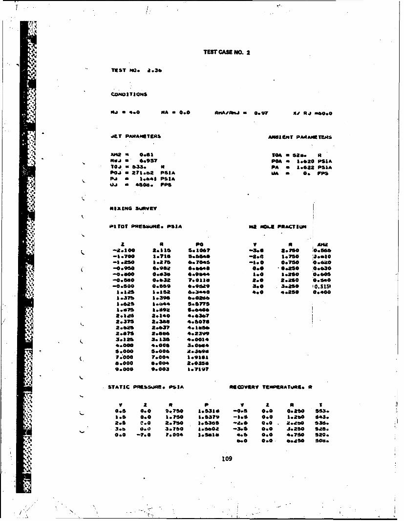
TEST CASE NO. 2

TEST NO. a.36

4 CONDITIONS

NJ a4.0 MA a 00 *nAvmq X-.94M RJ -000

JUT PA*4AMETEI3S AMIENT PARAMIETE34

AhM2 081 TOA = 2a 60-'. Nj 6.957 PGA = 1.s620 PSI^

*0Jin533. aI PA a 1 62 PSIAPOJ a271.02 PSI^ UA a 0. FPSPj 1.641 PSIAUJ -4500 FPS

MIM xING suiRvE

,bI 70 PROSSUME. PSIA Ma NO" PNACTIUM

z N4 pa v a AH8-10 2.115 603607 -see 20750 40..66

-1.760 1.716 sea&"6 -8.0 1.750 '30010-1.250 1.275 6.7046 -go* 0.750 0.060-0.950 0098 6.046 0.Go* 0.ese 0o30-o.400 0.030 6.9644 1.06 1.25 0.405

-050 0.032 7003110 e 2.0 2.5 IQ.$*0-00500 00659 6*9629 3.0 3.250 'O.S1S6311a &*Asa 6:3400 4.0 *.250 0.4000137b 1.396 0.0200.

2.325 2.140 4662.375 .2.366 4.50762.062 2o637 4.10562.675 28.6 402393.325 3.136 4.*00144.000 4.0006 3.0045.000 5.0006 A.36907.000 7.004& 1.916166000 6.004 2.03569.000 9.003 6*7197

STATIC PREbSUOM * PS IA INEOVERV TZIMPKRATURE. 01

v tp v m0.5 0.0 b.750 1.5330 -0.5 0.0 0.250 553.1.5 0.0 1.750 1.5379 -3.5 0.0 3.2b0 543.205 C.0 2.750 3.53*5 -As& 0.0 2.*sO 63603*b 0.0 3.160 &**b0a -30s 00 J0250 5460.0 -7.0 7.004 less&* 4.6 0.0 4.760 520.

0.0 00. "ASO0 500.

109

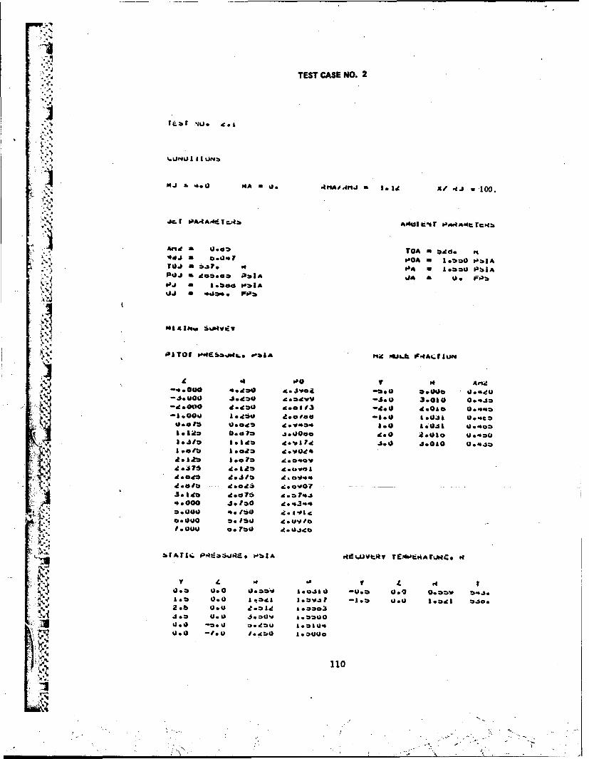
TEST CASE No. 2

AMJa.. MA 0. .4nAd.nja M o 10/4.Al 100.

1 A~ a 0.03 TOA . 4d

P t J a d m . 0 0 0 ^~J a * 4 ). O b I

PQ J IL 9Ooe PaIAU

PITOI 00b& nit~i. M31" OtfS&k "ACr1ut

'4PAO * Arftd

4U00 4649*0 Ac.adv -j*.0 3.000 0.*43O*a"00 At -490 ge.olIS -. 0 Q .0o&o Q.*4, 09 oa 1.~0 'e.0 too -too) &.041 .es.o15 & ad,2 41-0614 4;43 8.0 . U.00 1am 0.070 a.0060 d.0 aleuo U o 0 Q

*.Sft a 0 A4.*A0 46010 Q .q.1zIA %)solb lea43 d

O.475 do &.in0

d.4 soI* d 41 oa

3.14Id* .d7b .766000 4.130 o 63443.00 460 54) t48l 4

a aIWO 06150 4Uv1p t

as* 0 o70 0 *;# I o$ fp* 00 . b

-Ua

%)*a1 Pf~ 1J4~ O1 44JuacE~~4ru4.

WA'

a. V L 110

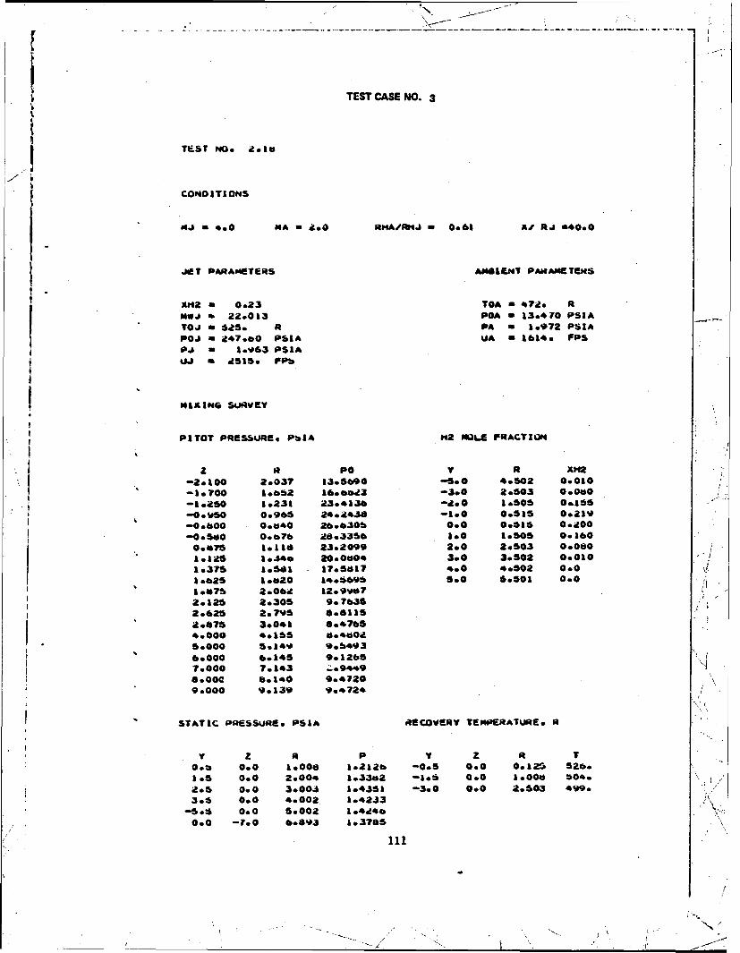
TEST CASE NO- 3

TEST NO. id.1*

CONDITIONS

mJ 40*0 "A 4 .0 RMA*blj 0061 Mi R -40.0

JET PARAETERtS AMBIENT4 PNAME-TIEWS

X"2 a 023 TOA - 47Z. RHui 22.013 POA a 13.470 PSIA-TOJ 6 25. . R PA a 1.972 PSIAP0oi 247.00 PSI^ UA - 164 FPS9.i - 1.93 PSIA

MIAING SUIAVZV

PITor PRtGs~uRas PbIA MZ OLE FRACTIkiY

-210 2e037 13.5690 -5.0 4.502 0.010-1.700 1.bb2 160"~3 -5.0 2.503 0.060-3.250 1.231 23.430 2.0 1.505 *&&be

-0%s 096 24.2438 -1.0 0.515 0.219-0000 0.660 20.0t30b 0.0 0.516 0.00o-0.500 0.b7b Z6.3356 3.0 1.505 010

00475 1.110 23.2099 2.0 2.503 0000

1.125 3.4 20.0004 3.0 3s502 0.0101.375 &*Sat 17.5417 ..06 4.502 0.01025 1020 14.096 5.0 5.501 0001.675 26064 z2.9vd72.325 2s305 9.76352o625 2&795 Goal&$

2.0475 3.041 a.47o54.000 0.165 0.4002a5.000 So.14%0 9.04936.000 0.145 9.12057.000 7.143 .*94498004 b.140 9.47209.000 9s139 9#.4724

STATIC PRESSURfS9 PSIA AU6COVERV TEN9ENIUtE9 Qt

V Z ftP v Z f T0.U 0.0 1.000 1&212b -0.5 0.0 0.1204 526.1.5 0.0 2.00. 1.33*2 -1.6 0.0 1.000 504.

g.$ 0.0 3.003 1.431 -3.0 0.0 2.503 4990

3.5 0.0 4.002 1.423-. 5 0 .00 5.002 A04460.0 -7.0 0.093 1.3705

TErT CASE NO. 3

TEST NUo 2.14

CCNOITlONS

NJ a 4.0 MA =2.0 RIA/RrtJ 0o60 X/ J . 100.

JET PARAMETERS AMIiENT PARAMETERS

-XH2 a 0*23 TOA - 472. iXJ a e0013 POA - 13.179 PSIATOJ - 523. R PA - lo9n2 PSIAPOJ - 2*7.16 PSIA UA - 1614. FPSPj a 1.942 PSIA

UJ - 2510. FPS

MIXING SURVEY

PITOT PiRESSURE PSIA H2 HOLE FRACTION

R Po Y R X-2-3 000 3019ts 20s4.b66 -3 ,0 2o4*6 010-2:000 20219 206*59 -200 1.450 0130-1.000 31275 2.0331 -100 0.47b 0.150

00ks7s 0.910 200105 000 0*570 001451.000 10119 Z.d740 lo 1*557 0.130

i.375 1.343 2.8465 300 30553 007010626 16674 40 13 400 4o552 0.0501675 1.811 2.7699 50 50552 0.0352.375 2.292 2.56872.625 2.635 2.59,U2.875 2.780 Z.86974.000 30d59 2*3979"6.000 b.b7b 2.3*39

STATIC PRESSUE PSIA RECOVERY TEMPeRATURE. R

Y z R P Y Z R T0.5 0.0 1001 1.1363 -0. 0.0 0o158 520e1.5 0.0 2.055 10212b -1.5 000 0.90 513o205 000 3.0:4 1.2b06 000 12.0 11.863 468.3.5 0.0 4.053 1.1913

-50b 0.0 4.952 10257b0.0 -7.0 7.171 1.26,7

112

TEST CASE NO. 4

T~T NS~e led

14J 4e A 4*j0 ol4Afwfl. a ..WK 4.1 alO.0

141 d* 1 a Pa 13.110 lai ATJai - 32o R P^ A.Vb.S PUIA

PU4 a ga4.ou PSIA 4AA A0446. P~bb,Pj a 1.66a PS15i a 3400. sibt

MUSING 5Oetvev

POITOT EPRZ.a6. PbSIA uia NOLA lVRA$..IUM

Y w-R PO y It AP14

;- *oy* 3dodbz1 0.* 0.0 .61

- 1 b .*4*6 00006

-tfo .027s~*V

-U.000 V.011

4. 1 3.000 U.10 0

0.0 - .0 000 1.7601

0.0 -1.0 A *ooo a.?~

0.0 -60 0.000 A. 1133

* 113

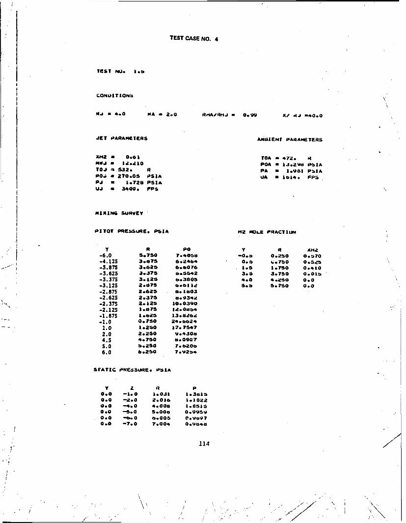
TEST CASE NO. 4

TEST NLo bb

I 0CNU1llTION4S

NJ U4. 0 MA 2.0 RrfAIfRtJ a 099 X.# PaJ a0.0O

JET PAARAMETERS AMaIENT PARAMETERS

XH2 a 0.61 TOA a 472.MWJ a 1J.J.l PGA - 13.29 PbIATOJ '532. R PA a 1.981 PbiAP0, a 270.05 PSIA UA n 1014* FPS

PJ n 1.728 PSIAUJ a 34000 FPS

MIXING SURVEY

PITOT PRESSURE. PSIA "2 MOUL FRACTIUN

y R Po Y R xa

-6.0 So750 7.4068 -00 00.50 0oe70-4.125 3.875 6.2464 O06 4;o750 0e525-3.875 3o625 *.a076 1.5 1o750 0.410-3.625 .3.375 *.56.2 3.5 3.750 0.01b-3.375 3.l25 oo3805 4.0 4 .$0 0.0-3.12S 2.675 601 I-' 5.750 oO

-2.875 2.625 fto103

-2.62S 2.375 0.93,id-2.375 2.125 10.0390-2.12S 1.875 14,. 004-1.87S 1a5 13*bits b6-1.0 0.750 24o624

1.0 Io2b0 17.7547

2.0 2.250 904300

4.5 4.750 u.0907S.0 b.250 Y.ob0o

6.0 6.250 70.92b.

SrATIC .'ESSURE. PSIA

v a P000 -1.0 1.031 1.3ts 15oo -2oO 2.016 olOA000 --4.0 400008 1.05150.0 -500 5.00a 0.995sh000 "6.0 6.005 eoo970.0 -7.0 7o0014 0.9a4

114

• • ' I "" f k " " . .. ,. / " . *'- ",

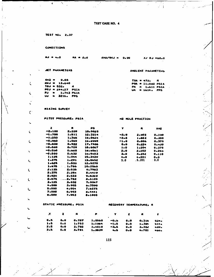
TEST CASE NO. 4

TIEST P40 2.3?

NJ S400 MA m 20 £AI'ofJ m0. 99 )to RJ AmO4sO

.857 PA*IAMETIER AMOS ENT PAI4AMETEsMb

E82 = 0.455 TO - 7ito IM.J - 13.640 PGA - 11.562 PS5410J - 32o it PA - 1.611 PSIAP0.8 m A44.27 PSI^ VA a 154. PS5Pi a 5e7403 P514UJ - 3216. PS

MIXING 5Uovey

95707 PMS-SSURS. P514 NQ2 MULA PRACT5ON1

-20100 2.209 10.9820-1.700 164111 12.3214 '3.0 2.602 49190-2.250 1.365 10.0824 -2.0 1.603 00300

C, -00.950 1.069 18.6990 -1.0 0.806 0.375-00400 0.922 17.7406 0.0 0.A22, 0..s0-0.560 0.709 58.0007 So0 1.204 0s,370-0.5b0 0.800 10.46661 2.0 2.202 0.26*-00500 00632 18.e9a03 3.0 3.202 0.110

1.126 1.044 15.3439 4.0 .0201 0.01.375 1.291 13.8652 5.0 S.201 .0.0lob"5 1.534 12.92701.615a 1.780 10.2585a.125 2.046 0679032e375 2.26.b 4.44192.026 2.533 906J232.875 -- 2o782 6.61093.125 39032 7.90474.000 3.905 6e75906.000 4.904 Ye.8757.000 6.903 6044410.000 7.903 801800

STATIC IMESSURS. PSIA MCC0VERV YEEAATmMIE. R

005 0.0 0.707 1.0560 -'0.8 0.0 0.316 524.1.5 0.0 1.703 91904 -1.5 0.0 1.304 U14.2.5 0.0 2.702 1.*010 -3.5 0.0 3.30it *6903.5 0.0 3.701 5.3839 4.5 0.0 .4.701 460

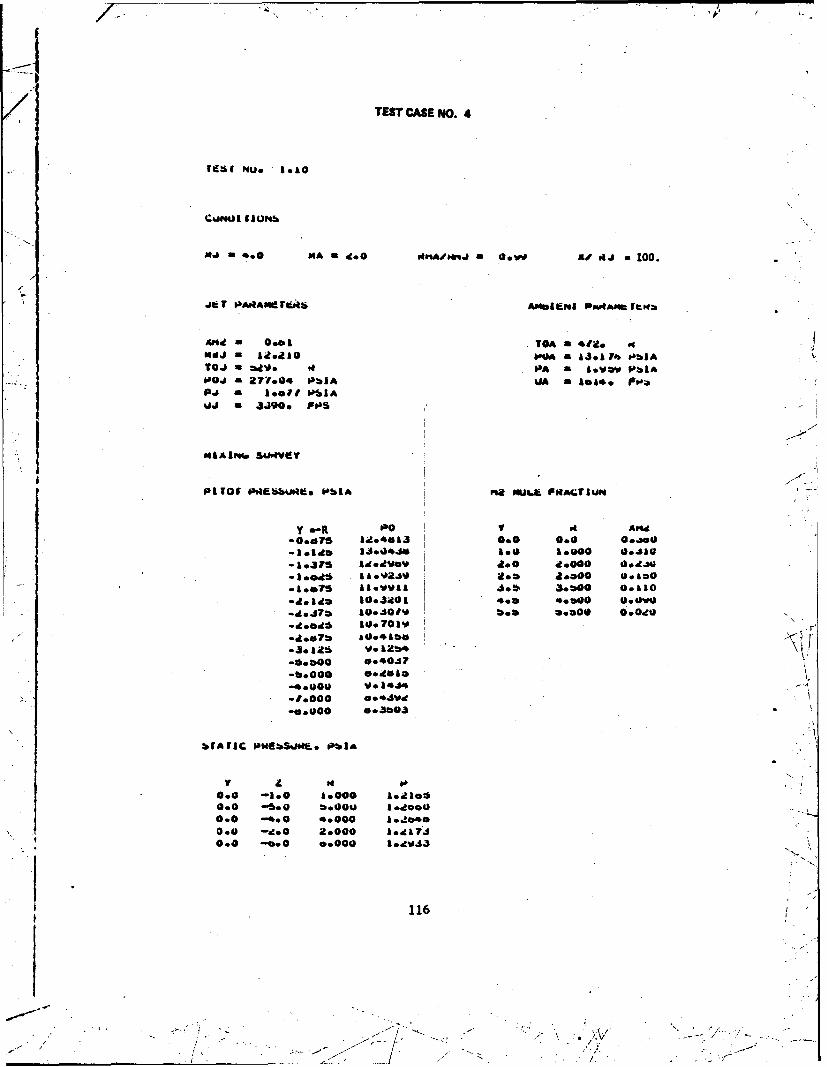
TEST CASE NO. 4

1IE.S MU. 1.10

Ca.nalI I umb

94 0 .0 MA d.~0 Nitni#Aj GOW sI 14 1 100.

JaiT POAAWerjS AMS1A PPAM.4A wb

And~ 0.0 1 .TO^ *Igo 0MaJ~~~A9 ft U.1 f4a J1' bIA

TOJ aad'. e PA &vow I~b1A0Ja 277.04 PbiA 4JA Ao* 1.1. 04

P.J a 1.011 PSI^vJ a JJ.90.0 FOS

SSAAIWNP SU.4VdY

P1101r PttI~ubi IbbA M2 MULU FRATIUM _

-047 14413 0.0 0.0 0.3.0-aeia J.~see5. 1.000 0.110

-1.vval JobVA 6 30b0 0.510-leliAd 10.305 .0 e.00 0.V

-i47 1.410bob **oo0000*d..i~ l0.701V

*.A2 V. Lb*

-boo** .14

-10000 *4.V-0.000 0.3003

bfAirC PfN1bSq*g*.. PblA

0.0 -1.0 A0000 1.ol~

0.0 -5.*0 d&.000 1,0400.0 -4.0 2.000 1.jb*@7,0.0 --f.0 0.000 1.iV33

116

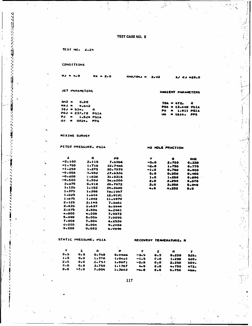
TEST CASE NO. 5

TEST NO. a22

CONDITIONS

0Ju . MA a2.0 n~ 2*93 X.4 itJ -20.O0

JET P.AAMETERS ANOIENT PAAMSETERS

XH2a 0.90 TA-42I4W a 54064 PA -0 13.*6 PSIAT~j 53. RPA - 1.911 PSIAPOJ 0 237.70 PS34 UA ft 1614. PSpj a 1*52~4 P554Uj - 55240 PS

MIXING SURVEY

PITOVr PRESSUAE. PSIA 142 MOLE PRACTION

z ft Po 6t ft-2.100 2.315 7.6068 -3.0 2s766 0.330I 1&700 1.718 l0e74" -2*0 10750 0.770

-00800 4,0836 31.8318 Soo 3.250 0.890-0.00o 0.559p 34.*000 2.0 2.250 0.570Oeo1 00910 28o7872 3.0 3.250 0000Is12b 1.152 24.36WS5 4.0 4o250 0.01.375 1.3983 16.19b?1.625 10644 12.91911.675 A .kl92 11.49792.125 2.140 7o6#361

*2.62ti 2o637 6059442.875 2.886 6.2461-b.000 *.008 7.9?072

5.000 5.006 7.9596

9.000 9.003 SO.49"

STATIC PRESSURE. *SIA RECOVERY TEMPERATURtE* f

'IY z It £ l0.5 0.0 007b0 0.V486o -0.6 0.0 0.250 525.-I3.5 0.0 1*7'10 I.0.ga3 -1.5 0.0 1.250 520.

*2.5 0.0 20753 1.0871 -2.5 0.0 2.250 bo09.3.5 0.0 3.750 3.1767 4.5 0.0 4.750 472.

I0.0 -7.0 7.004 3.389)3 -. 0 0.0 6.750 46.

117

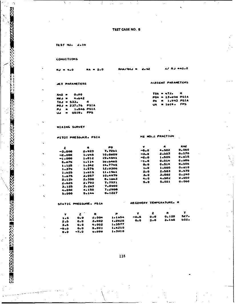
TEST CASE NO. 5

T1ST We. id.1

CONDIIONS

NJD 4.0 NA -2.0 RKA/RHJ - 2.V A/ Ri M40.G

JET PARAMETERS AfMSKENT PARAMETERS

X~i2 0.90 TOA - 472. R

0MVj 4.642 POA a j3.09d PSIA

10.5 - 533. . PA M 5.943 PSIA

P0.5 a 237.76 PSIA VA a 1oi4. FPS

Pi5 n 1*546 PSIALDj a 59. FPS

NIAIN. SURVEV

.'ITOT PRESSOME. PSIA 12MOi,4 FRACTION

-3.000 2.923 7.7261 -5.0 4.502 0.060

-2.000 101045 100009 -3.0 aqb03 0.570

-100 102 1061-0 16505 0.615a lo~^06 100 *514 0.906&*&a 1*42 3se745 00 0514 0.906

1.:iw 1.576 12:9P306 too0 &*SOS od

1.026 105 1161901 2.0, 2.503 0.570

1*075 2.057 10.4979 3.0 3.502 0.240

2olb Z300 Gla3 40 .502 0.050

a2.6Wa 2.790 ?77471 5.0 5.501 0..060

3.125 3.2b3 7.09004.000 4*150 7.2t9005.000 5.144 6.1227

STATIC PRESSURE * PSI^ geCOVERY TEMPERATURE* R

v P v z R T

1.5 0.0 il.004 101654 -0.5 0.0 0.120 527.

2.5 0.0 3.002 l.2da8 0.0 3.0 3.160 502.

3.5 0.0 4o002 1.3577-506 0.0 5.001 1.42100.0 -7.0 6.090 l.3910

118

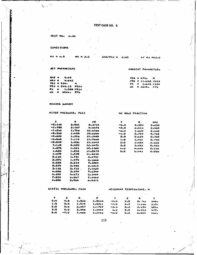
TEST CASE NO. 5

NJ a4.0 "A a .0 .AMA/R1J d o%03 A-* tJ zo0J.0

Jet PAA~TERS AMSIEr4T PAA4EtR

X12 m 0.90 TO^ a 472. RmwJ a 4.642 630A -11I.*b3 P'xIATOJ - 534. R PA -1.5l1 IlAPOJ - 240.10 PSIA UA AL £614o t*P5iP3 = 1.500 psi^v3 a 65240 FPUS

MIXING SkmVey

P:TOT PR~bU~ PbIA H2^3f FRACTIUPN

z R laO I R AHt2-2.100 2.544 0311b -5.0 4.59V 0*260-10700 2.1*7 d.ab7b -3.0 2.61* QUso-1.2*0 10744o 10.0oebo -460 16039 0.000

-090 1.459 16ave -1.0 0.y2%0 0.750*-00400 1.316 11.3405 0.0 0.015 0.750o

-0.500 10110 11.7*o6 14.0 1.4vi 0.140-0.500 1003b 110OV40 2.0 0.6 O. co0

*16195 00600 14.s*17b 3.0 3.452 0.4b*S.375 1.021 1*.1346 4.0 4O.**~ U. 1 *1.625 1.262 k11.26 73 5.0 b.441- 0.0tob1**75 1.4%p0 11.0210

2*37Z 1.975

2o625 2.219 7.33k§48.875 2.04 CI b543*125 2.112 1* 19204.000 3e5S79 7.e-34V

5.000 4.*74 04

7.000 *.5*7 7.4403V0000 80564 c4.03wv,

STATIC PREbSUME. PSbIA AFC~ftNv TEMPERAIURtE. R

0.5 0.0 lookm 1.013,4 -13.b 0.0 0. b,3 5*k.1.5 0.0 10914 1.00b1 -1.5 00 1.100 5j32.5 00 2.957 1.1 7%P7 -3. s 0.0 J.109 bob.3.5 0.0 3.94b 1.2*4 4. Z 0.0 4e.9.1 4617.0.0 -7.0 1. 4*5 1.42 . .0 b 40-1.

119

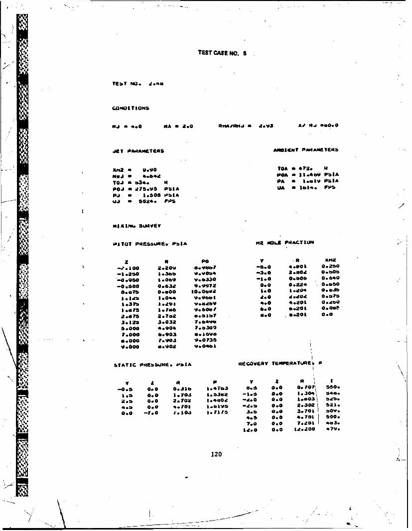
TEST CASE NO. 5

GONON TIONS

NJ 4" A - . #AH 3Af NJ -0000

AM2 a .90 TOA M 7. IAMUJ~~~PO M .4 10 11-4W9 PSI

j a *34* 14 PA a 1001V PSIApJaj g75.V5 PS1* UA M F04. PS.

Pi a 1.500 lob"A

DITUT PSIIS*UNE. PUIA "a N062 P.ACTIUN

Z N PO V NZl

-0? 100 2020*0 4.90.7 -6.0 4.001 0.260

-16250 10300 ipovo*4 -3.0 2.0o 0.b06

S-106 00006 0.40

10.97 0 1 009 . 633 0 04 .2016 0 0601.4150 1.16g 9.007 106 1 .20 0.0490.475 27 0.00 1000%.0 4.201d 0.07A30126~ 1.032 v. -ft 140

Io.00 A*de A.0 1.oa30'40I.o 0,

boors Io903 V.160 0 .0 00oek

5.000 4.903 7.0390000 4.903 6.0041

STATIC P"ZIbWUMd .'sIA I6aCgVany TftfRTURZb

pVI A A P.10; ft0I

-00 0.0 0.310t 1.4763 0.6 000 @1 ~50&.s 0.0 16704 1.6302 -1.6 0.0 1.304 :$48.

2.5b 0.0 2.702 10404 -. 0 0.0 1.o03 b626.

4.3 0.0 4.101 1.01V -g.5 0.0 2.302 Sa1.

0.0 -700 11 1.7116 3.o 0.0 3.701 Mov.4.0 0.0 4.701 500.

7.0 0.0 7.got *o03.12.0 0.0 u2.200 47V.

120

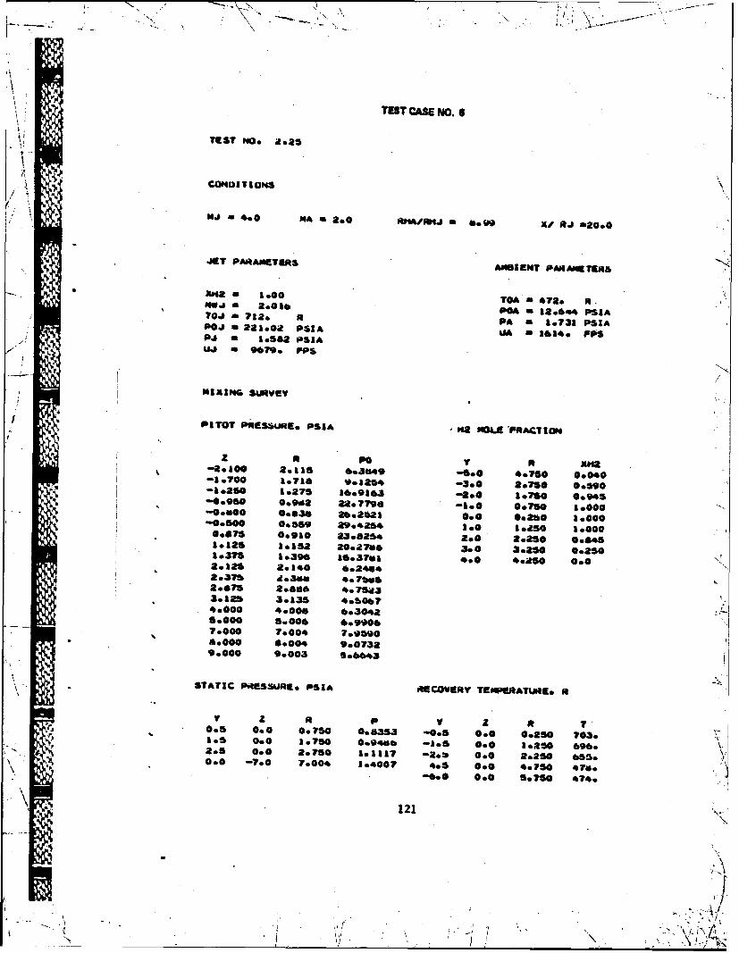
TEST CASE NO. 6

TEST "as. a&25

CONDITIONS

NJ o" A a200 hRt/t /J -2000

JTPARAMETERS AMBIENT PARdIMasE*

X"2 0 160o TOA a472o N.MWJ - 2.0 30 POA Is 38.0.4 PSI^

Toj - 120 aPA - 1.731 PSIAPOJ -221.02 PSIA UA U 1644 FOSPJ a IoS82 PSI^lU - 9079. FPS

MIMING SUV

PITOT PPSzmmK* Psi^A09 'MO LZ PRAC II

-210 2.115 6*3449 -00 4.750 0.040-lo700 1.718 9.1254 -3.0 2.750 0.990-10850 1.275 60.9503 -2.0 10750 0.945-00960 092 2776-1.0 00750 1.000-0.8600 0*83 26*2b~i 0.0 O.2b0 10000-**a"0 0.559 29.46254 se0 3.250 1.00@0.675 0.930 23o&264 2.0 2.250 00643.325 38152 20.27160 3.0 3.250 0.2501.375 3.396 15.37.1 4.0 4.250 0.02.125 2e140 6.2442.376 d&300 4*7bob

S2.075 2o86 4607S;933.125 3.135 4.2.0074.000 4000 0.30426.000 5,000 6.99067.000 7.004 7.95900000 0.004 9.07329000 9.003 Sb"

STATIC PRESSURE. PS1K ONCOVERY TEMPERKTUR.5. N

I z R P R, T0.5 0.0 0.750 0.0L353 -0.5 0.0 0.250 703.3.5 0.0 3.750 0.946 -1.5 0.0 3.250 90-A2.5 0.0 2.750 103117 -200 0.0 2.250 65g.0.0 -7.0 7.004 3.4007 4.5 0.0 4.7540 476.

-0 000 5.750 44

121

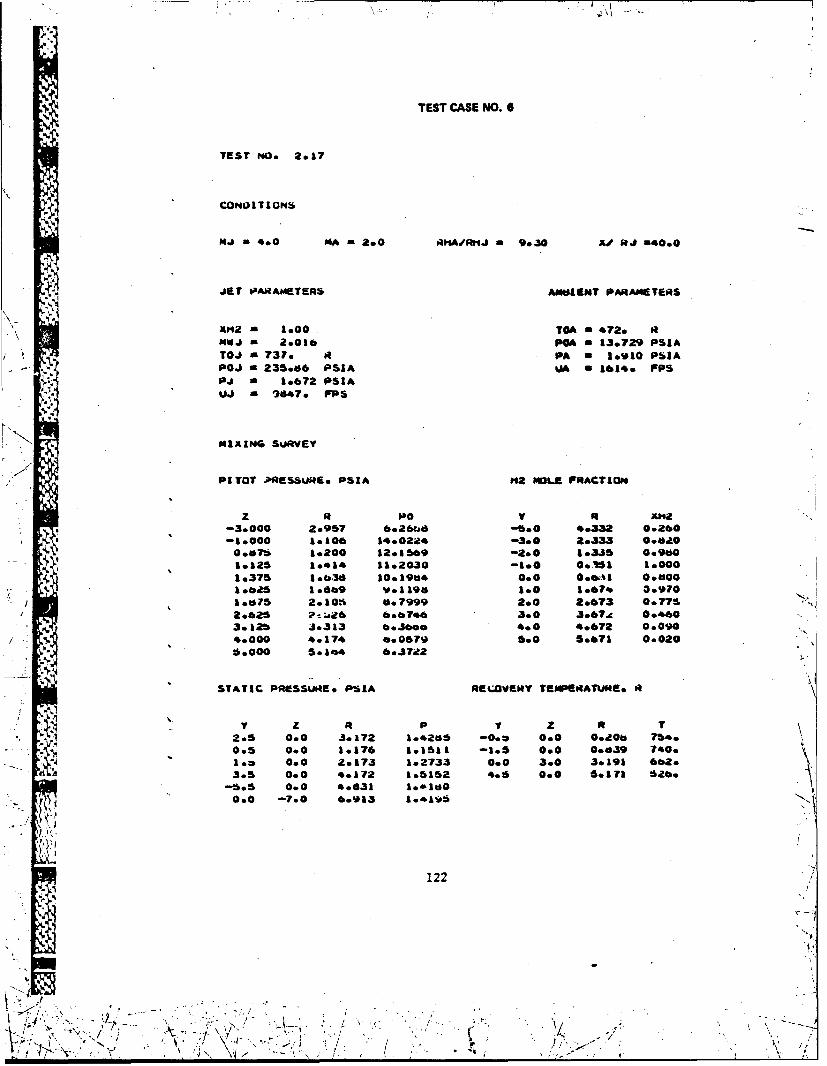
TEST CASE NO. 6

TEST NO. 2.17

CONOITIONS

NJ a 4.0 "A m2.0 .aAflRtJ n 9.30 A** RJ -4000

JET IARAMETERS ANUIENT PARAMETERS

XHa - 1.00 TOA a 472o R14MNJ L 2.0016 POA U 13.729 PSIA

TOJ - 737. a PA W I.910 PSIAPOJ 0 235.66 PSIA VA a 1614. FPSp.i = 1.672 PSIAUJ " 2847. FPS

MIXING SQRVEY

PITOT ,"ES. PSI^ H2 MOLE FRACTION

Z f 1'0 R ft 5M-34000 20957 602 , : 4 *.332 0260

o| 0000 It0o106 14*02.14 -3o 0 ao,;'J=J, e04,10

0007b 10200 12o1569 -200 5.3..5 0.9"10125 1414 11.2030 -100 O.WI 1.0001.375 106,36 10.1964 000 0ow1 0 0.001o.a25 10669 o1196 1.0 1.67, 0910

o6ST 2010.o b.7999 2.0 2o673 0.775a.625 6.1746 3.0 3067.g 0.460S3.125 .5.313 6.3600 4.0 4.672 000.

40000 4o174 660579 5.0 5.671 000206.000 5.1ft4 6..722

STATIC PRESSURE* PSIA REC.OVEIRY TEMPERATUREe A

Y Z R P w Z t T2.05 0.0 .5.172 1.428 -0.0 00 00.011 754.

005 0.0 1.176 1.15 1 105 000 0.639 740.loo 000 2.173 1.2733 00 30 30191 662.

3.5 000 4.172 105152 40 0.0 60171 2o.

-'505 00 4o831 I1.aI0000 -7.0 6.913 1.4198

122

4 :

'K!-. -: <+_. "+ o i '" '42-,/ *

. ,+ + :, ,} + -+ - p ,. , .. *

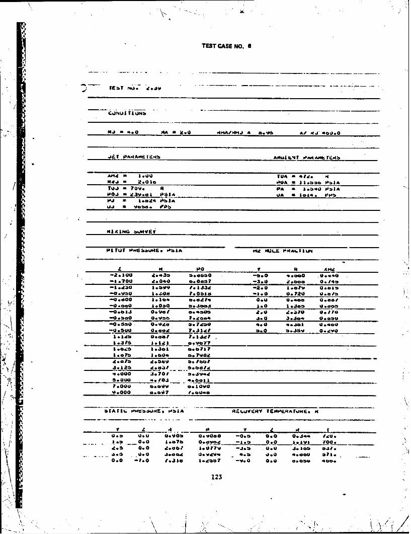
TEST CASE NO. 6

FEbIT iou'. Id.Iv

;JN*U 1 T I um

NJ a*0 ~ a0 v4nANtIJ dqv 0.$ . J 0.0

J41I PAAd14kb AAUdt4r eDAR.AMtTEAL.

AP12 160 TU ~A a*14do Pt

TJ - .0. a PA A 1.04 O 1A

PoJ n-i 30.8 I SI VPIAh, at iL. a - PbJA

41A IN(. ImMVEI

PITUJT Ob&~~E.~ A I1g F4ULA b II1

-20100 Ae..J0 *Saoa -0.O %.0000 .. *-A.700 it*040 o.o7-3.0 20600 0. to*-1.0 1.0a I 09 tIJ3d -Zoo I.DIV 0.010-0 evou I*-,on 1.0040 -1.0 0.120 .o-0.800o solo* 0. odif, 0. U.00 0 .0-0.040 A 0000 **Jooa4ko I. 1.4am .

-0.0. ioct 1 0.0$ 46.0 46310 .,-0 .0 boo aa tomb oo4 Sea0 3.4o* .U

-0.SO 005w a*74z 4.01 4.401 a.0-0 a 00 0.00,d 7041'er 0.0 5035v 0.adeo _ __

I.s a Lm ebl 70 1 4dd

I0046 1.3.1 0.0171.070 1 .0* be.70

5*000 40661 1.v*

P.000 o0oav 0'.1 ova0.0000 o00 1600-46

@AItir1*14E P in"lA R&E4LLuVd.N TEAILA f4do It

0. o ou 440go U. v00 -00* 0.0 fe1u.a* 0.0 1.07b 0dd A 0.0o a.wl 00

.0 0.0 5.obb: 1.017V -Jam 0.0 Jo.lob 041.-.. s 0.0 Jo" 0ewS.. %.0 0.0 do *?I00.0.0 -100 1.310s l.do7 -v.0a 0411 00000 400.

123

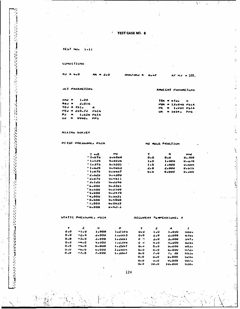
TEST CSE NO. 6

TIb t Nu. 1 .11

i MS 4.0 14A A t.o oA~ -6 Af Pdj a 100.

AH2 a 1.000 TO^ 4140.

Ma1 -* a i01 1VA -I.4 kTOJ - 75I 1 4 40A a 1.003 PbiA

Poj 4bo 79 ut^UA a 3114 FOU

US A 99400 epu

PAFO 101 bcsi PulA n.a MU F.Am;Tluf

- 1.a7m :2.009 .00 0.0 0.100- I' 6*"f 1.0 10000 U.0fU

- .016 *3041 105 soo ;o.4bb

I.0 Od 04oj d* t00a1~

',deal *.4Oa0I

ep.000 030

0.0 -0 ~000 00 .0-.00 /c

0.050 d.0 .000be

0.000 0. b.00 01

0.0 -10 000 .d dto 0.0 100 lU.OU 0.

0:0* -4: -*0 ~!* .- j 500 aU0 04

. . . . . . . . . . . . . . . . . . . .

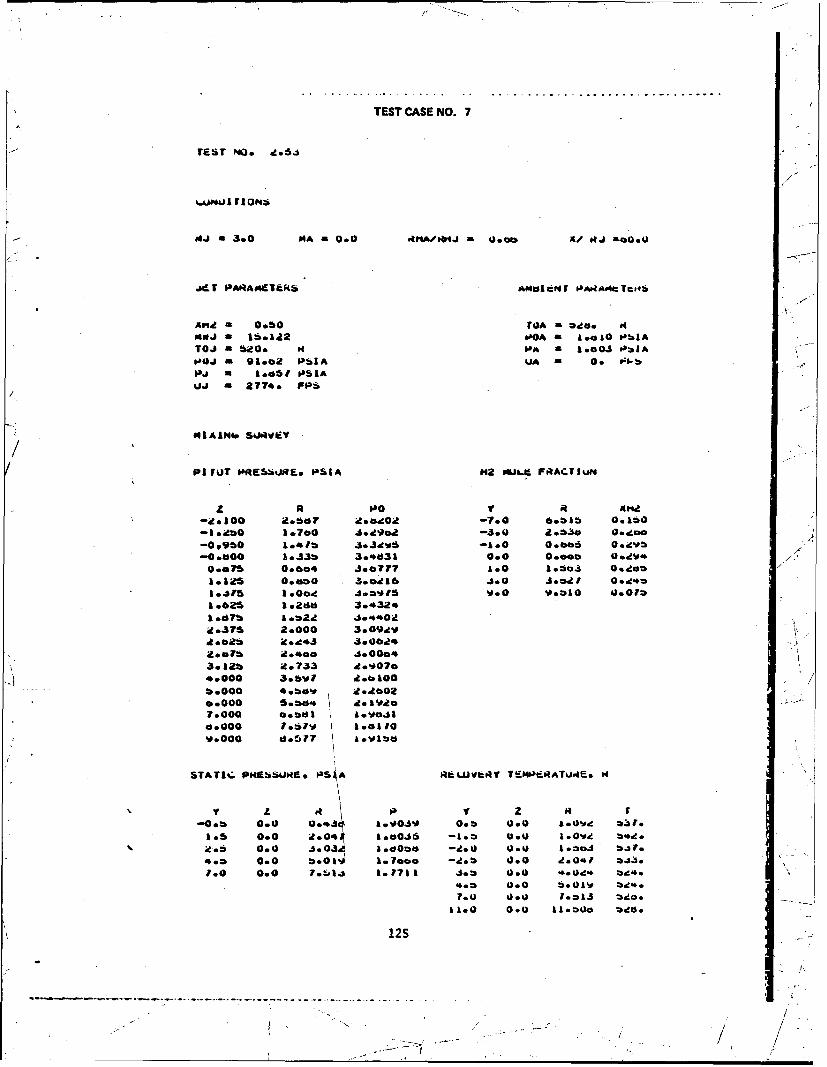
TEST CASE NO. 7

TEST No. et*5

A J n 3.0 MA 0.0 vthA.iblJ X/ Li' Nj -O00

An42 0.50 rGA n mdo. atMUJ - 16.122 0hA n lool £0 $IA105 520. It PA a 1.003 t PI A

OJa91002 PSI^ VA M 0. 01-I~j- 1.061 PS1A

%11 2774. FPS,

MIAIN4. SORWVV

PI~u f~ ESSURE9 PI^1 M.2 MULA FRACTIuM

I Go0 2.567 ;2.ad02 -7.0 6obib 0.160-1 oidu 1.760 As.20o -3.0 2.54. aoo-09950 1041b joJdtw6 -1000 0 60:5 0.2v8b

-0.600 103b 3o443l 0.0 000@ 02i07

0.0Th 0.604 Sea???Lo I. 1.403 a0.do*10125 00a50 3oo26 Jou 3.821 00.40

1.62$ 1.248d 3.4320

id.37$ 2.000 3.0920~2.t2o ;9.943 3.0824

;966 A o400 s.00odb3012b id.e733 do-A07*.b.000 3.ol 2.0100La

b.000 4.840. 9.40020.000 S.ftwb 2102a7.000 0.*o1 1.0.41l4.0000 1.:b10 1.81,%00000 do5~77 1u o

STATI%; PRtEbSUM~o PIA RkiuJVe~NV I *ptiA1UAN0 N

-a.* 0.0 0.434 1.04,0 0.8 0.0 A1.002 8sf.1

1.5 0.0 Z .0% 1.60.6 -1.8 g.o 1.0ye 84..

2.8 0.0 3.03 1.001 .2.0 0 .0 1.*.4 U4.3

4.8 0.0 8014 1.7ooo -,do8 0.0 2.0461 *.34.1.0 0.0 7.tols 1.1711 3.8 060 .024d 8*.

.8 0.0 b.030 82.0

7.0 40.0 1.813 z20.

&1.a 0.0 11.*00 Z00.

12S

TEST CASE NO. 7

TEST NO. Z5o

CUNOK TIONb

4J, - .3.0 "A 0 .0 RHIA/Ri~j a .b6 X/ 14J =00.0

JET PAR.AMElTERS5 AMIElNT PA.RAMt:TERt)

an 0.50 TO^ - Sea. Rt

WJ, 16.12 POA & 1*750 PSIA

10. U 3e R PA - 1.73V PbIA

P0.5 a .19 P!3 IA UA a 0. FPS

P3 1.85* PSIAU.5 27a2. FPS

MIXI3NG SOVEY

PITOT P$esswme PbIA H92 MU~LE FR4ACTION

z R .'

-2.100 1 .. 31 2.3'421 -0.0 *.Zdb Q.lbb

-1.250 10127 2 *16 Sa -3.0 2*630 0.1soz-0.950 0.dbs 2.42z1 -1.0 00569 0.194

-0.kia0 00745 2.4bo0 0.0 0.s3z 0.a1ISod0.d75 1.00 2.41d7 1.0 1 .*941 0.195

1.12b 1.436 e.'4014 .4.0 3.'46d 0. 1 ti16475 l.675 e.3639 6.0 0.4t14 0.1*

12 1.916 2o.4,3 b.0 0.6 0 1 id

2.375 2.4b49 4.ds

3.125 3 3dY 2.24o3'4.000 4:457 do 1500b.000 5.252 200036b.000 b.!40 'd.00307.000 7.2*o IVO

ti.000 8.24&69.000 9.2'.2 1 .4943

STATIC P#kEb5u~e. Ph IA RECOVERY TEM4PERATRE,~ R~

V Z R Y z R r-0.5 0.0 0.231 1.7S14 0.5 0.0 1.007 5212.1.* 0.0 1.99.5 1.7704 -1.ti 0.0 1.04b 5,eZ.

.. 0.0 2.9#b9 a. 7bv7 -,do0 0.0 1 .5.3f *..

.. 5 0.0 '.985 1. f324 -2.5 0.0 2.033 b23.

0.0 -7.0 *.7t57 1.72w1 3. t 0.0 3.VO7 2'4.'4.5 0.0 4.0* 3,o

7.0 0.0 ?.4'&co 5ib.

le.0 0.0 12. &O' 5,e5.

126

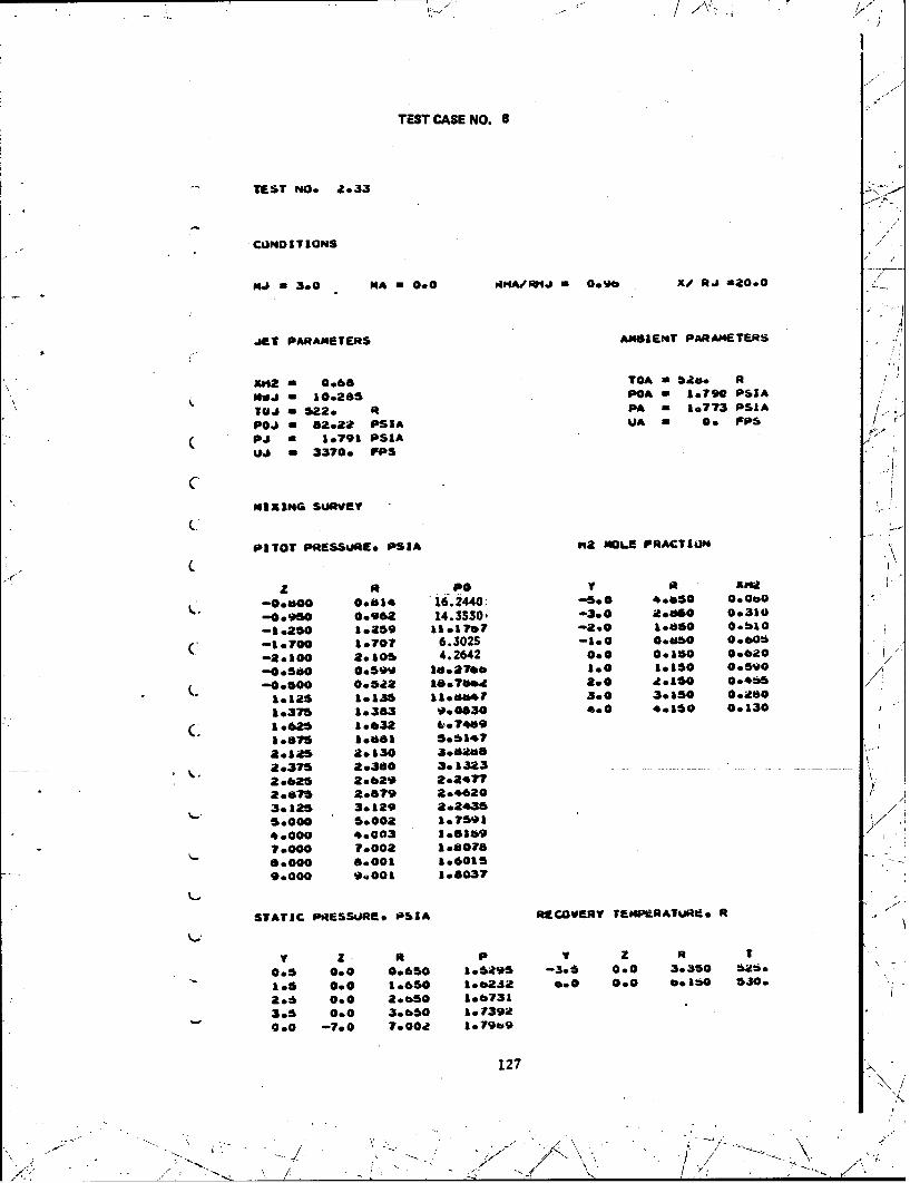
TEST CASE NO. 8

TEST NO. A.33

C43HOSTIONS

NJa3.0 MA -0.0 ~ I1/tJaOV i RJ -20*0

JET PARAMETERS AMOZENT PARAMETERS

MWa 066TOA a 546. ftXS42 a 10.28 PC^ a 1.790 PSIA"W0 1285 ftpA a &0773 PSI^

p03 62.2a PSIA UA W 0. fps

pi a .791 PSIA

01 3370. FPS

MIXING SURVEY

PIlOT PRESSURE. PSIA via MOLE FRACTIO3N

-00660 0.614 16.2 440: -4.0 401650 0.000-0.960 0.962 14.3530- -3.0 a.460 0.310

-1.250 1.259 %s.o t -2.0 1.050 GeblO

C- -1o700 l.707 6.302S -1.0 ombo 00605-2.100 2.105 4.2642 0.0 0.150 0.620

-0.00 0.59*0 10*2764b 1.0 1.150 005%) 7(-0.500 0.522 10.764H 2.0 46150 0.465

1.125 1.185 s1.dU4? 3.0 3.150 0.200

1.375 1.363 9p.0630 4.0 4.160 0.130

C;1.625 1.632 4o7409

l.675 &.*"1 5.6147a.125 2.5340 3.0266

*2.375 2o360 3.1323

*2.625 2.629 2o24772.075 2679 Z.46203.125 3.129 2.2435S.000 5.002 1.7591

4.000 4.003 163697.000 7.002 &*more6.000 6.001 1.6015

9.000 9.001l &.6037

STATIC PRE-SSURZ. PSIA RECOVERY TEMPERATURd. Rt

Z . it P v z ft T

0.5 0.0 0.650 1.o5sail -3.5 0.0 3.350 batio

1.5 0.0 1.650 1.6232 0.0 0.0 0.160 530o

2.6 0.0 2.oS0 1.6731

3.5 0.0 3.650 1.7392

0.0 -7.0 7.002 1.7969

127

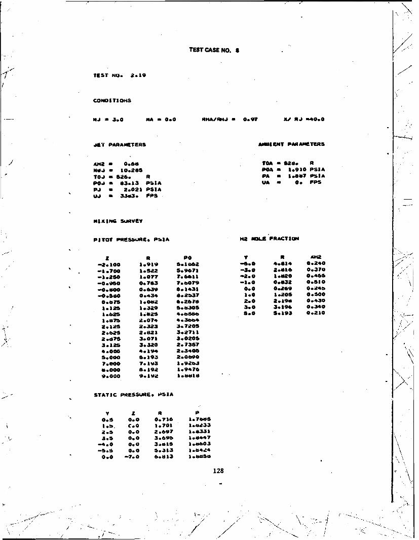
TEST CASE NO. 8

1> TEST HO. 2.19

COHOI TI 014

NJ 3.0 M4A a0.0 64NaI~j 0.97 AdNJ =4000

41LY PARAMETERS AMID ENT PARAAMETERS

AH2 a *6 TOS. - 626o R

Md4 a 10*285 PO5 a 1.910 PSIA

TOJ - 526 R PA - 1.007 PSIA

POJ - 83.13 PSIA UA 0 00 FPSpj a 2.021 PSIA0i a 3303 o ps

MIXING SLAV5'f

PITOT PRIESbUAe. PblA Ha MOLE FRACTION

-20100 1.919 S.1002 -00 4014 0.240

:1:700 1:5412 :0671 -3.0 2.016 0.370-125 l07 T661-a** 10820 0046s

-0.960 0.783 7.6079 -1.0 0.632 0.530

-.00800 0.639 0.3*33 0.0 09269 6624b-0.500 0.434 G.2b37 zo0 1.205 0.500

0.675 3.062 6.2676 2.0 2 &190 0.430

3.120 l3.9 Seb305 3.0 3.196 0.340

1.625 &**as 4.6666 5.0 5.193 0.2101.4675 id.074 4 036642.125 it.323 3.72052.625 2.0521 3o27319*2675 3o071 3o02063.125 3.320 2.73574.000 4.1" 2.3-0055.000 G.393 2&0607.000 7.163 1.92b36.000 a o194 1.9476*.000 901wit l.6616

STATIC PRESSURE* PS1A

*0.6 0.0 0.710 1.7665lob. coo 3.703 1.odt33as& 0.0 2o697 1.6331.5.5 0.0 3.696 1.6.47

--4.0 0.0 3*065 366603-5.6 0.0 5.313 10042~40.0 -7.0 6.613 1666546

128

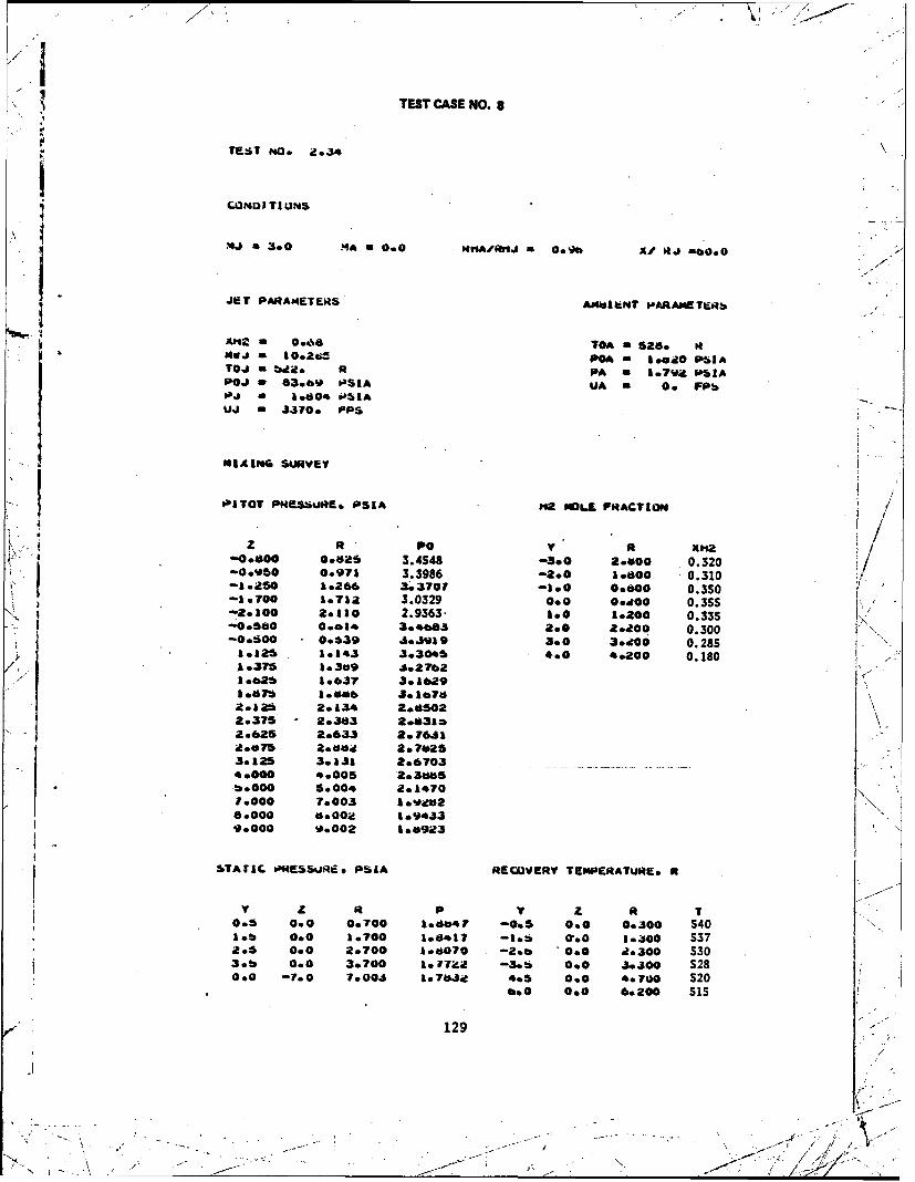
TEST CASE NO*

TEST ftO. 2.34

WONW I UNS

300 s~ MA -0.0 RHA.*I;J a @.fo Xt b4j ao

9JET PARAMTER4S Aso1 iNT 64ARAEE~

Mica- 0.66 104 - 528. H414gj a 10024M PO4 1 *4.20 PSIATOJ -b42. R PA a 57V& PSIAPoi 83.69 PSIA UA a 0. Fpb

uJ a 35370. FPS

NI1AING SURVEY

PARTaT P,4E5SURE6, PSIA M2 MOL.L FR4ACTION4

z PO Y R 2-00800 0.0"it 3.4548 -5.0 20000 0.320J-0.950 0.971 3.3986 -2.0 10800 0.310

-A 0250 1.266 3o370? -100 0.800 0.350-1.700 1.712 3.0329 0.0 0.200 0.355

K-2.100 2.110 2.9363- 1.0 1.200 0.335-0o.s00 0.014 3od&68 2.0 a*.200 0.300-00600 0.539 .5.3*19 3.0 3.2006 0.28S16125 1.143 3.30*5b 4.0 4.200 0.1801.376 ls359 .S*27621025 1.037 3.1029

i2.128 2.134 Ze.85022.375 2o383 2od3Io2025 2o633 2e76451

050.0 0700 1.84 -05 . 030 40.0 0.0 100t t .o1g--60G 330 3

0.5 0.0 0.700 1.6070 -0.5 '0.0 0.300 530lob 0.0 3.700 1.6*72 -1.5 0.0 1.300 5280.0 -0.0 270. l.7032 -2. 0.0 ii.700 520

0.-0 0.0 6.200 515

129

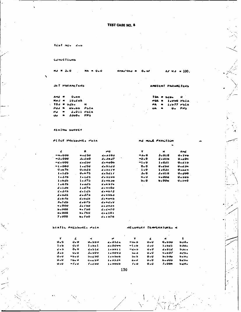
TEST CASE NO. 8

144T mI. eeo

(.iNUIT~umb

pNj 30 .0 aAaUO n~ 0.v -it 44 100.

Jtr T A ~m -~ Amd1ftmr PAA.T

Me j a ods OQA U. 1VGPl

M aJ a zz.d R PA u *V ?0 bLA

poij a UV0 plA a 0. FPS,

%"- J~aOA FPS

-*AI4 a iso . FP

Pirur P mb*%J~t~q pa lsk Vid .. a.A PFM*4f1r , -

PO I 0VI And4.00So 404~. 1~04 -. 00 400 ev

-4.000 J.£, .SJ -. 20b .O

-1.00I &.,60 .oA 0.0 0.Q U.44.

&.4T7Sbj b.0 1A0o .440

1.did m

0.000 zi. 150 447.000 cb. 100

^T Ll..~ a4~ ~I pAE6..UVLEq rb~ 0,tI 4

0.z -0.0 1.041 e.oV-6 . . 104 .V

d. b db4 LVI I -eo 0. .19 *aa

t7 . $-1* -00 *e*-IV0

#j 0U -OU Ormu .1003-6Uu 0-J/______ _____ _____ _____ /_. _

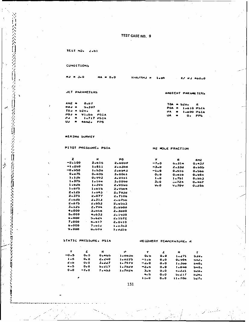
TEST CASE NO. 9

CUNUITIONSp

MJ J.4 0 M* A =0.0 RrIA/Rr1j I 1b4 X/ 1*4 MC2.0

jET PA1*AMEThRS AMOtIENT PAhiAmferRb

£112 a ~ 07 TOA - bU. hMwi .397 POA - 1-1 PbIAroi a24. hi PA - 1-009 PSIA

P4a9::507 PSIA UA m Q. FPS,a,3j a 1717 FaSIALi a .ae FPS

M41 N~i~ SURiVEY

PIVOT P1*SWR1E9 PSI^ H12 AC)L. FRACrIUN

-2100 2.416 2.00. 70 b.3014 0.431

-3.07 22.70.66

t ~4000 0.635 2300100 044 .51.002 0093 2.101 . 051*375 6. aa4 3.00cs30 .74Z.a

6AIC .0*1 10*39 4.ERY TEM.0 R 9*0 . a

3.61 a1 03~ 1.191'4.15 1.3 2. 93a0.07 2.7 it. 70b

2:04*5 2.313 e. 131

TEST CASE NO. 10

TEST NO. gob

CANOLTIONS bO

NJ a 3S.0 MA -o 0. nAi4mnJ 6. o13 -6000

JTPA.4AMTS ANUIENT PARtAEER

532 1OG T"~Sw R-PsiA m 1.r20 WSIAIiTOJ -659. R~ PA U 1.64a I*AA

POJ = sVb PblA UA a 0. FpbPi a 1.749 PS14

j n 650. FPS

1ISsim4a SURVftY

PIVIJI PRE.iije PSI^SI MD"I FRACTILIM

Z600 Ae5 2.a4 V .4-00950 1.*7 .2.00? -3.0 42006 0.646

J:.3:Z iold 11111i Iii0 I:0I2 0971bSTATI0C50 at 70" 1*0~A TPRAoU.4S 00t

10Aa4 0. 0 2o7537 0 300 3.432 0619.

1.37 0. 04 2.6. 71.1 - 9. 0 1.332 00426

102.5 007 3.3*6 143 -20 0 12.3 022.0.0bf led&* 2.a.o -. . 216 6

3.14 0.030 2.O7377J

is. 0.00 13.3* ..0010 8033128

y /

TEST CASE NO. I

JE:T mul. 2.32d

1/ CONDI TIONS

NJ a 3.0 MA 2 .0 nA#*R'j 10.00 X-4 RJ -20.0

JET PARAMETERS AMWIENT .OARAAMO TIERS

39"2 a 1.00 TOA = 472. RMJai & 2o01 POA - 13.043 PbIA

*T0J a 62a. a PA 1*724 PSIAPQJ ft 91.4? PUIA UA a1614s FPSP3J a 1.856 P51AUJ = ?6660 FPS

MIXING SURVEY

PITOT PMESSAE. PSiA M2 MOLA FRACTION

-2.100 2.107 0.5*33 -5.0 4.030 000-1.700 10700 ag0o a -3.0 2.830i 00460-1.250 10262 12s1395 -200 1.630 oedoo-00950 0.96b 1406491 -1.0 0.030 0.0-0.b00 0010 10.02W2 0.0 0.170 @.95s-0.580 0.604 l7.1266 1.0 1.170, 0.9b0-0500 0.52od 17.4ga0 2.0 2.170 0.7551.125s 1.134 1 Ileos 3.0 3.170 0.1401.315 1.385 9.05&77 4.0 4.170 00010625 1034 7.95341k.*75 1.0,3 7eleJ6

2.125 2132 5924752o375 2s361 4.*35792.0241 2.630 4.470A.815 2.00 b*43523.195 3.130 b.11814.000 4.00.6 8*.7937.000 7.004 9.2101s0000 60002 10%3V99.000 V0002 9.79,02

STATIC PRESSURE* PSIA RSECOVERY TEMPERATURZ. R

v P R T006 0.0 0.670 1.0164 -0.6 0.0 0.330 b20.1.5 0.0 10670 1.2121l -1.5 0.0 1.330 536.2.5 0.0 2.670 1*5051 -2.6 0.0 2.330 520*3.u 0.0 3.br0 1.7749 --Jos 0.0 3.330 407.0.0 -7.0 1.002 1.7"X5 6.0 0.0 6.170 5vse

133

TEST CASE 1NO.11

TEST W*. z.20

CONSDITI ONS

-~-MJU30 MA a2.0 RA/fRIJ A 10000p RJ "0.0

jig PARAMETERS NITPA MCE

- .0TOA a 42s RA~a m 1000poA n 13,603 PSIA

lovi w 2.016 *a W

TOJ - 626. R I'A a1604 PSl

pOj a *.46 PSI^ Aa164 P

Pi a 1,831 PSIAuJ a 7656. FPS

MIX ING SURVE'

pilaf PRESSU~t" PSIA Pea MOLE FRACTION

z it ebo -0 4,7 0.20

-20100 1*727 ToO073 0.25

7o.125 3.663**3 .454.*000 1& 6 -200 10*4

-1.000 0099a %*770710 061 .1

7000" e752 ooW 4256 00 0426*6.000 Oo*2S 064

9000 9.oo I9.0253

10066 006 9*.207 20 .9 o7

12.2 0.047 0.8 *.3.5S-4.0b 0.3o3? "34

0.0 -7. 5 6.7577 4047 0*0

2*704 * 134

Z02 3- 92 630

TEST CASE NO. 11

TEST ND* 2.3b

NJ a 3.0 04A -2&0 fa/4J a0 9v'o oi I 640.0

JEV PARAMETERS ANUIENr PAI4AMETERS

*H auz 1000 IOA = 720

Mw a .010 POA a 133016 PbJA

POJ a07*3 PSIAUA a1014. bPJ a 1.759 PIo4J a 7620o FPS

MIXING SURVEY

PITOT PRESSURE. PSIA n2 NO&E FRACTION

-2.100 aegis 60053 -3.0 !20750 0*606-10700 107140 6.0776 -2.0 0 007bb

-5.250 19275 0720 -100 00750 0.*"0-0.950 0096a 0969 Go0 09250 0.00

-00600 0.036 6*0731 1.0 I.0450 00600-0560 0.032 606lbs 2.0 12.250 0060u

-0.500 069 6.7536 3.0 3.450o Oobiol.5a5 10152 041b0 4.0 ;40.tso 0*406

r1.310 1.396 6.35641.025 1.644 0169110475 10#92 be323321li 2.140 050002.375 2.04 04202.025 2.637 5.03252.o7S 2.0160 5.'*4223.12b 3o&35 Soa4.000 4.0060 6*124756004 5.000 6.13627.000 7.004 6.040*

9.000 9.003 004665

STATIC PAES:5JE oPSIA RECOVERY TEMPERATOR~e R

v z0 00 00750 0.00 -0 s* Od*O 5b

3.5 0.0 3.760 130 -lb 000 IA b7

t0.0 -7.0 270 3.4f35s -. 5 0.0 4.750 410.

0.0 0.0 0.250 %6i-I 13S

TEST CASE NO.. 11

o ,TfibT vi.e .

q 4Ja s. 'IAU ~. 4nANr. %)*d.o A/.j 100.

Jt.T PhA~AAETEAS AbarU.A4MI.4

An1d U O.00 TC0*. *I~d. itg~ja do.016 POA 0 1490 Pbt*

TOJ 3~j IDA a IV0Pblik

PUJ dg.4-A P$LIA V* - lot*. rFa

A' J ,05. Fpto

* ~z .1 pu 1 04 A .

4~"4000 7-.0 4.4410 0.4o*040

-3*000 J.004 0.00a1 -JOO A1.-40 0u.*30

-10000 1.100 *. d0oe -1.0 0.4010 u.b*00.61M 1.001 0. 00-61 0.0 00000 0..340

I.7 a 'd 1.0 7 0.1011 100 A.60011 0.*Im

1 37 10*0 ou J00937-6

A O.0a 4 04 S4 -640 Oio.07* so.JU e-$

A. I6 e U. 00U *..o0 -0.e 0.A.00 !

,d.b1 0. 40 3.u I I-soIJ.: 0 O.100 .*0

0. 00 .0 3.04 d I.A1I*1 ~000 -0. 0040 I4~

05 -. 00 :3. 1 U,01

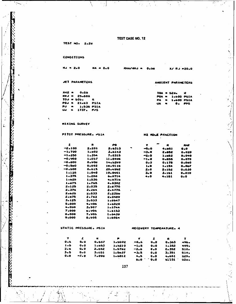
.7

TEST CASE NO. 12TEST '40. 2.2e

CONDITIONS

Ns J a 00 MA a0.0 RbiAmj a0.bd X/ NJ =20.0

J1 PARAMETER~S AMBI ENT PARAMETERS

X04 **a& TOA a bas 143

POa 21.03 PI a 0. FPS-j 1.5368SA

UJ - 1737. P

MIXING SURVEY

PITOT PRESSURE. OASIA H2 MOLK FRIACTION

-2.100 20201 2*6313 -s.0 *ws 0.0-1.7Q0 10602 3.8143 -3.0 2.8652 0.020-10250 16354 7.0315 -2.0 1.652 0.040'0.960o 1.06? 13.049a -100 0.855 0.070-00600 0.00I 14*!32b9 0o0 0.176 0000-00500 0.692 16*9116 1.0 1.154 000o-0.500 0.815 20.*b902 2.0 2.152 00016126 1.040 10.0091 3.0 .5.161 0.0301.375 1.286 6*9714 4.0 4*161 000I1s026 1.536 46V7161.0575 A1o7al5 4.03022*125 Zo035 2.07702.o375 2.2054 2&47762.825 i9.533 2.236*2.a75 2.70$3 2.04693.125 3.033 1.08*750000 4*4006 1.a8020g4.000 3.907 1437447.000 6.00 1.616360000 7.105 1.64309.000 80905 1.6054

STATIC PRESSURE. PSIA RECOVERY TEMPERATUAE. A

Y R P I z R TGo 0. i 0. 0.8:51 1.0592 -0.6 0.0 0.363 496oRes 0.0 1.853 1.0210 -1.5 0.0 1.353 499.2.b 0.0 2.852 1.67ne -2.6 0.0 2.352 510.

*3.5 0.0 3-4b~l 1.5.37 -3.5 0.0 3.351 519.0.0 -to 0 7.0906 1.8012 4.5 0.0 f&.661 529.

137

TEST CASE NO. 12

J TEST '40. 2.21

CUNUITI UNS

]MJ 2.0 MA a0.0 ~ AARrij a06 X/' pJ -4000

:..T PARAMCTbERS AM8I ENT PARAME TER~S

xn2 m 0.083 TOA - ?8. R4WJ - 25.8t8b POA = 1.660 PSIA7~j a 515. R PA - 1659 PSIA

Poi a 11019 PSI^ UA a 0. FPS

P.) a 0.876 DSIA

U.) a 175. Fpis

MIXING URE

PITOT PRES6U.RE* *PSIA H2 MOU.. FRACTION

-2.100 to.93 3.31.31 -. 00 4.316 0.02,

-1:700 1.0b24 3.7171 -3.0 2.321 0.03,--1.250 1.2.31 4.4398 -2.0 19330 0.042

-0 . %05 0.997 46 305 0.@ 0.727 G.ft-0. t%0 0.o595 4.7674 1.0 1.706 0.040-0061 $ 0.774 4.799b 3.0 3.697 0.0;d0

0.a7b 1.303 4.00%0

1.125 1.521 3,907b

2.215 322.454 2.459

2.6Z5 .937 1.685

1.b? 0. 8 .02 .540

2.06 0.0 e 19 1. 6394 i.5 00 .0 2.19 l.30

9 -. 00 0.025 3.416 1.a20.00 -7. 260 l6 oOV

U.000 ti-.!.

__ __ __ __ __ __ _ __ __ __ __ __ _ __ __ __ __ ___STATIC__ __ __ _ PR SS RE /I

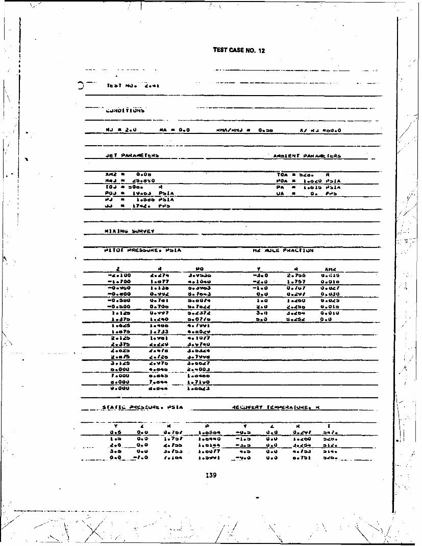
TEST CASE NO. 12

MJ a 26) 14A a 0. 0 04fAdhNiJ 00*0 / ~moe

jtf PAIAMETtift A04MAIENT P~^t M.

X442 0000 Tot% a *o R'40J a *dUa OA a 3ecO0 ft-LAI0J *000 It PA a &gt OblAPoi a j.04 PbIA UA m 0. a

ObIt

g.0 dd' Svbjo -4.0 2.* 0041%i-110 .*77 .01060 -zoo l.T7 0.010

-0l0oaaft a. oa..3 01.0 00101 004, 30

-O.oe 0.701 6.00140 o Iebo 06040

-000 070 UevV odd4 3.ea ie.,db 0.010a a ag I.vV7 6.0937A 3.o Jo* 00 4

2 Idtf level 411

goals del .fe so 7Vvd

00000 00640 20*0041000 o.04.0

460001) 7.06

Lob a 0. J.?al 1.oc'0 -ISM 00 1.400 O

de* 0.0 gola eatd *. 0.0 J. :6 0I'd

3a 0.0 J.la . £.0i7' c4 0. 4.la. ICJ .0.0 -1.0 gl.A04 £.*VvA _*.0 0.0 a~i bb ~

139

TEST CASE NO. 12

Iib MU. d.V

fIJUpw1 h1I mb

NJ. do d0 MA 410.8 P4tA/r"iJ Oo 0.O Ad' PtJ a 100.

JiEI PARAMIET~lf A14CIENT O4AMrTh~

Arid 0.OaTO^~ - Dec.- 14J adzoebu .p0A a 10720 P~SI^

TQJ - *40. ft PA a 1.14* P~xi^ilhoi a 11.00 PSI^ Ja a,0 FPJS

P.8 - 1.101 PIA

UJ = 177be FPb

MIAING 56IMVEI

Pi rtr Potbme Pb1,m me ML= IiAClLU4

L atm~0y And-.4410 Sc3m I1e1L? -6.00 4~d .

-4.000 466,411 I.V1 10 -4. 0 2.4 d 0*deI-. 00 16010a &.,p*43 -doU Iob~e O.UdvI.

-1.000 0.Fw In a -A3 -two 0.040, 0 0.00.475 1 oU V-41 as U 000-60 0 .0.3A 0iz a00 Sou 1.0 1 0*5 0 . zoJ

1 .4 It 1064.6 I.-Mid 3.0 J.*4~j U.Jda

4.0 *.*1* .d

d *Iith d.*.4 0.5v1 ~ 0 .d

d.4/z 4duO 1~OJoba 3.0o I 1.11J

3o lif J.o 1.0901.0041 4.6d@ I a I0

U.404 5.4.d0 1.od,*7

4rAf1c )Ads~oatc. PSI^

.3 0.0 .1. ad1 1. Ida-

0.0) 00U 1.7 1. 7 J-

140

TEST CASE NO. 13

TEST No 2.31

CONDITIONS

N4J 26~0 "A -200 RAII elA ~~

JET PARAMETERS ANOINT4 PARMETERtS

£12- 0.96 T0£ - 472. R

Nwj a 3.212 P0A a 11.575 PSIATOJ m *JI. PA a 1.701 PSIAp04 a 21.80 PblA UA - 6*. FPSPj a 1.379 PSIA

a. 5067. FPS

NIAINwi SURVEY

PIlOT PRESSURE* PSI^ 042 I4)L. FRACTION

z R PO Y 14 142-?*Soo 2.191 7.00d3 -!400 4.751 000-1.700 1.794 V.6300 -3.0 9.751 0.370-40,250 1.350 16.6910 -2&0 10752 0.766-00950 1.057 20.4246a -1.0 0.754 0.926-0.00o 0.912 22o3305 0.0 0.202 0.965

-00500 0.703 'd.o6059 &*a0 1.252 0.Ods-0.500 0.629 25.3706 2.0 2.251 0.600

1012b 1.077 1601240 3.0 3.2b1 000&o375 1.322 12.4543 400 4.251 00010625 1056d %#o4323

1*075 1.615 7.8l6id6/2.12b 2.063 5020792.375 2o312 4.0267 X

___2.676 a.809 b.1006

3.12b J0058 6.04:534.000 3.931 *.**Its50000 4.929 b.06167.000 6.9025 6.6186#&.000 7o.9.7 6.400990000 a97 666

STATIC PRtESSJRE9 PSIA jjEWJVERY TENPERATURE* R

0.5 0.0 0.764 0.b~bo -0.6 0.0 0.262 614.-1.* 0.0 1.752 1000 -to* 0.0 1.2WE 6260

2.5 0.0 ;do 51 1.1216d -Z.5 0.0 2.25L al7a

3.5 0.0 3.151 1.326 -3.5 0.0 3.261o 4v0.

0.0 -7.0 7.Oal 1.60464 40b 0.0 4.751 479..0 0.0 bo.260 466.

141

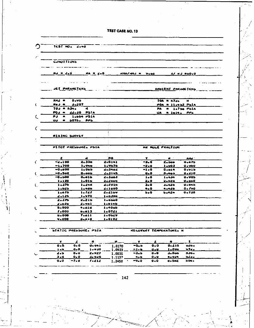
V/

144 " . A 4.~0 UI/4 ~~A.# PMJ -n0.0

JET PAR#%4dft~b A04VaAELr P0AMA~ftfff

N.*J - 4.00 poA a I1.*b3 Put^AlOj aSq 63 St PA - 1.?*o PUIAPOJ a Ag.S0 PSI^ UA L 1* 14. Flab

( PJ a 1*6 PSI^u4J - 6076o FP

MIXING SuitVay

b& TOWr O~~~kj OLA "Ad 04u" F9MLTtU"

Z . PO v 04 AVZ.lo 2330 204141 -3.0 2*660 usfth 1

-1.700 t.0fe 1.-At76 -200 1.03 0.OiUQ-00600 A Obb de30 -1.0 060440~

-Oso 0.600 4!413%0 0.0 0.ft03 00010

.. fitf 00640. I

Adolt, o7 '.00 3.02*Jbt 20210 1.&4000 44~ .

6.0 6.2 1 166146

5000 4.61 I.Oot*000 o.d13 *7t66000 70011 h.0bavVe000 &.1 .0192

0.5 0.0 0.941 1.0170 -0.0 0.0 0.216s o.eo

dom 0.0 2o.027 1.0935 -3.0 0*0 .o. 6450030:5 0.0 .s Vdt 1.1137 .3 0.0 .J 0.2.3.000 -7.0 1.*1.u 1. 24SO0 -w.0 0.0 6.6"2 6000

142

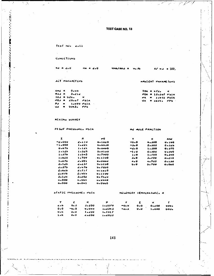
TEST CASE NO. 13

a4 d 0 A d.0o".tl a V.1b X/NJ au00

J...T ,4i AM131NT PAAMefI~b

An~d O:V* TOA a 4610.5 2 I' PA a 13.4*7 A -I.

I oJ w POA - I.JO l

* MIALN~a b UVeV

PjLIr Pwb~m "bZA ng MjLd FiRAQTAUM

k.76uids V 06.IlG -SOO .3.iO0 4I.&1

3104 1 e 76 0.14.000 jlo jO' 4.*?*0 e. 00 O.V04.4 ---- -- I 43

0.0O0 U.000

1143

-600 -6. .cI **-

./

APPENDIX II

BOUNDARY LAYER MEASUREMENTS

I

I4

NOTE: * Measurements are presented by increasing Test Number

9 See Table V for the cross-reference of Test Numberto Test Conditions

I~144

'. . ,. : / I/ :..

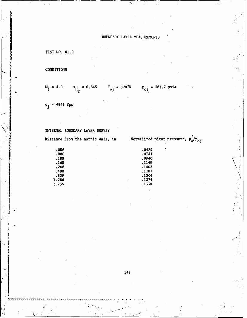
BOUNDARY LAYER MEASUREMENTS

TEST NO. 01.9

CONDITIONS

M =4.0 xH2 = 0.845 T = 528*R Poj = 381.7 psia2 0

u = 4845 fps3

INTERNAL BOUNDARY LAYER SURVEY

Distance from the nozzle wall, in Normalized pitot pressure, po/Poj

.056 .04F9

.080 .0741

.109 .0940 .

.165 .1149

.248 .1403

.498 .1307

.839 .13441.286 .13741.736 .1330

'1 145

U ".

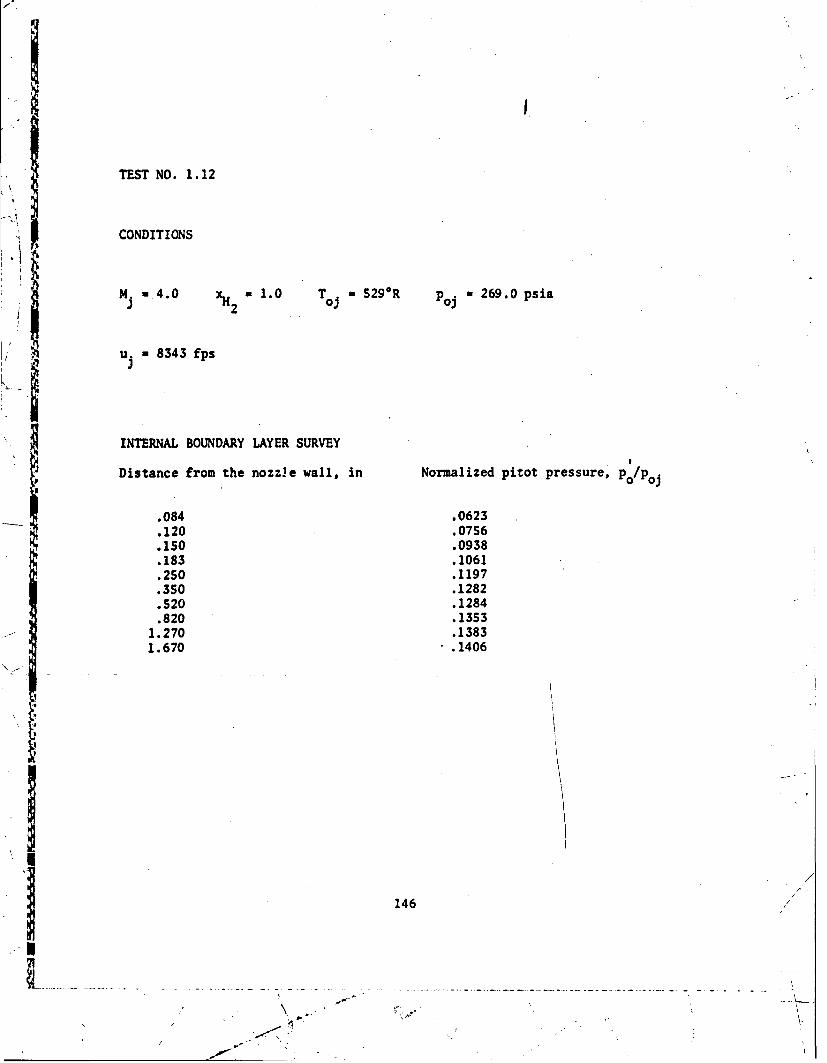
TEST NO. 1.12

CONDITIONS

M. u.4.0 xH a1.0 T0 .5 29OR p.j 269.0Opsia3 2u. 8343 fps

INTERNAL BOUNDARY LAYER SURVEY

2Distance from the nozzle wall, in Normalized pitot pressure.-, /0 o

.084 .0623.120 .07S6.150 .0938.183 .1061.250 .1197.350 .1282.520 .1284.820 .1353

-1:270 .13831.670 .1406

146

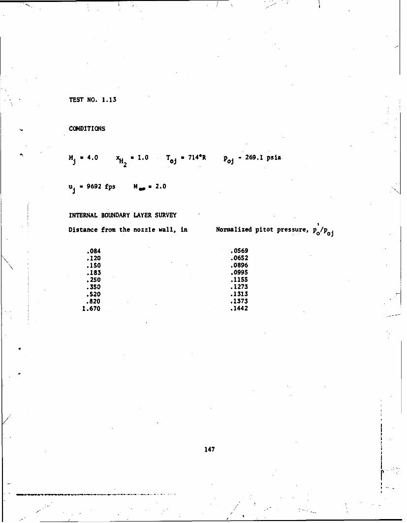
TEST NO. 1.13

Cc*4DITIONS

M.4.0 *H 1.0 T * 714*R -o 269.1 psia

u j .9692 fps Mew 2.0

INTERNAL BOUNDARY LAYER SURVEY

Distance from the nozzle wall, in Normalized pitot pressure, p/o

.084 .0S69

.120 .06S2ISO .0896.183 .0995.250 II115.350 .1273.520 .1313.820 .1373

1.670 .1442

147

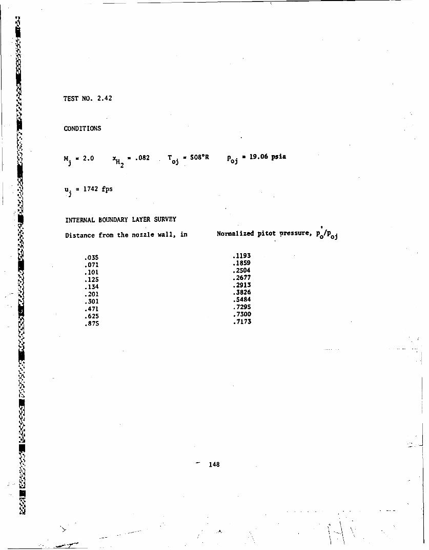
TEST NO. 2.42

CONDITIONS

M. .082 To - 508R p 3p - 19.06 psia.XH2 oj

u. = 1742 fps

INTERNAL BOUNDARY LAYER SURVEY

Distance from the nozzle wall, in Normalized pitot pressure, po/Poj

.035 .1193

.071 .1859

.101 .2504

.125 .2677

.134 .2913

.201 .3826

.301 .5484

.471 .7295

.625 .7300

.875 .7173

IJ

148

N ,;

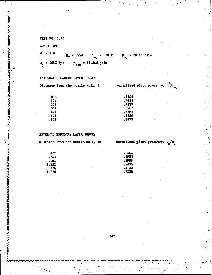
TEST NO. 2.43

CONDITIONS

Mj a 2.0 XH u .9S4 T S30°R P 20.83 psia

u. = 505& fps o 11.368 psia

INTERNAL BOUNDARY LAYER SURVEY

Distance from the nozzle wall, in Normalized pitot pressure p /p0 P oj

.035 .3356

.101 .4422

.12S .4359

.301 .S982

.471 .6362

.625 .6259

.875 .687S

EXTERNAL BOUNDARY LAYER SURVEY

Distance from the nozzle wall, in Normalized pitot pressure, po/po

.401 .2363

.6S1 .2982

.901 .39551.151 .S49S5.276 .61227.276 .7238

149

2Jtrl-t /°ltvrfna. ~a,%- na ~.is . ~tatt n . a. .- . .a. '. . . ~ - -

TEST NO. 2.44

CONDITIONS

M. 3.0 H .682 T. 524*R p0 95.11 psia

u. =3377. fps

INTERNAL BOUNDARY LAYER SURVEY

Distance from the nozzle wall, in Normalized pitot pressure, o/o

.029 .0721.06S .1338.095 .2004.128 .2S89.129 .2683.295 .3348.379 .3327.465 .3267.629 .3266.879 .3284

1.615 .3321

150

...... .....

.... !/

TEST NO. 2.4S

CONDITIONS

M. u3.0 XH2 31.0 T oj. 524R Pou 98.23 psia

u. * 7627. fps P0 0 13.026 psia

INTERNAL BOUNDARY LAYER SURVEY

Distance from the nozzle wall, in Normalized pitot pressure, Poj

.053 .1424

.089 .1980

.104 .2091

.119 .2851

.152 .302S

.319 .3303

.354 .3267

.489 .3210

.604 .3237

.854 .33051.639 .3291

EXTERNAL BOUNDARY LAYER SURVEYi!

Distance from the nozzle wa11, in Normalized pitot pressure, po/po

.333 .2363

.S83 .2779

.833 .36601.083 .48441.333 .54463.208 .7444S.208 .70167.208 .6822

- , ,. , ,./ ., " ' "'.9 '

'II. '

TEST NO. 2.46

CONDITIONS

M . =4.0 x .553 T .- 527*R p. 273.7 psia

u. =3201. fps =o' 11.430 psia

INTERNAL BOUNDARY LAYER SURVEY

Distance from the nozzle wall, in Normalized pitot pressure,P0 i)

-1.022 .0451.053 .0S60.088 .0813.121 .1004

- ~..129 .1072.288 .1381.379 .141S.458 .1386.629 .1385.879 .1395

1.608 .1384

EXTERNAL BOUNDARY LAYER SURVEY

Distance from the nozzle wall, in Normalized pitot pressure, po/p0

.058 .. 2603

.308 .3035558 .3628

.808 .43801.058 .54131.308 .63785.183 .69256.183 .69407.183 .7216

152