turbulent mixing in a tubular reactor: assessment of an...

Turbulent Mixing in a Tubular Reactor:Assessment of an FDF/LES Approach

E. van Vliet, J. J. Derksen and H. E. A. van den AkkerKramers Laboratorium voor Fysische Technologie, Faculty of Applied Sciences, Delft University of Technology,

Prins Bernhardlaan 6, 2628 BW Delft, Netherlands

DOI 10.1002/aic.10365Published online in Wiley InterScience (www.interscience.wiley.com).

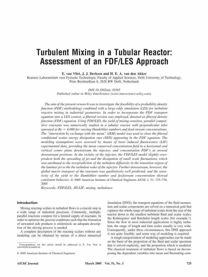
The aim of the present research was to investigate the feasibility of a probability densityfunction (PDF) methodology combined with a large eddy simulation (LES) for turbulentreactive mixing in industrial geometries. In order to incorporate the PDF transportequation into a LES context, a filtered version was employed, denoted as filtered densityfunction (FDF) equation. Using FDF/LES, the yield of mixing-sensitive, parallel compet-itive reactants was numerically studied in a tubular reactor with perpendicular inletoperated at Re � 4,000 for varying Damkohler numbers and feed-stream concentrations.The “interaction by exchange with the mean” (IEM) model was used to close the filteredconditional scalar energy dissipation rate (SED) appearing in the FDF equation. Themodeling assumptions were assessed by means of laser induced fluorescence (LIF)experimental data, providing the mean conserved concentration field in a horizontal andvertical center plane downstream the injector, and concentration PDF’s at severaldownstream positions. In the vicinity of the injector, the FDF/LES model slightly over-predicts both the spreading of jet and the dissipation of small scale fluctuations, whichwas attributed to the overprediction of the turbulent diffusivity in the transition region ofthe laminar jet to the the turbulent wake of the injector. Further downstream, however, theglobal macro transport of the reactants was qualitatively well predicted, and the sensi-tivity of the yield to the Damkohler number and feedstream concentration showedconsistent behavior. © 2005 American Institute of Chemical Engineers AIChE J, 51: 725–739,2005Keywords: FDF/LES, 3D-LIF, mixing, turbulence

Introduction

Mixing reacting scalars in turbulent flows is a crucial step ina wide range of industrial processes. Commonly, multiple,parallel reactions compete for a limited supply of reactants. Inorder to optimize the process conditions such that the formationof unwanted side products is minimized, an adequate descrip-tion of the mixing process is needed.

A complete description of the reacting scalars without anymodeling can be obtained by means of a direct numerical

simulation (DNS); the transport equations of the fluid momen-tum and scalar components are solved on a numerical grid thatcaptures the whole range of turbulent scales from the size of thereactor down to the smallest turbulent fluid and scalar scales,the Kolmogorov and Batchelor length scales [for example,1].Since the flow in most industrial applications is highly turbu-lent, the range of length and time scales usually is very wide.Consequently, under these circumstances, this DNS approachis not quite feasible, and some way of modeling is required.

A rough categorization of modeling approaches can be madeon the basis of the proportion of the fluid and scalar spectrumthat is solved explicitly, and the proportion which is modeled.The classical treatment of turbulent flows is based on decom-posing the dependent variables into mean and fluctuating com-

Correspondence for this article should be addressed to E. Van Vliet [email protected].

© 2005 American Institute of Chemical Engineers

AIChE Journal 725March 2005 Vol. 51, No. 3

ponents (Reynolds decomposition). Models are required toclose the cross-correlation terms that appear upon averagingthe decomposed transport equations. Consequently, suchRANS-models should cover the whole spectrum of turbulentscales. Since no distinction is made between the large andsmall scales, the models have to capture two distinctly differentphysical processes; turbulent convection at the large scales, andmolecular diffusion at the small scales.

Mechanistic micromixing models rely on the idea that mo-lecular diffusion and the resulting chemical reactions take placeat the smallest turbulent scales; therefore, the advection-diffu-sion-reaction equation for a scalar within an assumed laminarflow field representing lamina in a single Kolmogorov eddy issolved explicitly [for example,2–4]. As a consequence, a sepa-ration of scales is incorporated into the mechanistic micro-mixing model; the high end of the scalar spectrum is solvedexplicitly, and the cascade from the large down to the smallscales is modeled. Usually, computational nodes that representthe locations of the reaction zones are tracked within the flowfield calculated separately according to, for example, a RANS-approach. Dedicated models are adopted to capture the turbu-lent cascade of the reaction zone in order to predict its currentlength scale. The micromixing advection-diffusion starts at themoment the Kolmogorov length scale (or some other scalerelated) is reached. Since the result of the approach depends onthe way the complicated and nonuniversal cascade process ismodeled, one could wonder whether it is useful to put allcomputational power into the numerical solution of the scalaradvection-diffusion at scales that are predicted so crudely.Moreover, at the moment of release of the computationalnodes, it is not known a priori what the Kolmogorov eddy sizewill be, since it depends on the turbulent region where it willarrive in the reactor. Since the initial properties of a computa-tional node depend on their unknown future state, micro-mixing models are non-causal, and, consequently, it is inprinciple not possible to set the initial conditions (such as theamount of reactant dye fed to the reactor).

With a large eddy simulation (LES) approach, a low-passfilter is applied to the transport equations of the fluid and thelarge-scale motions of the fluid are solved explicitly. Modelingapplies to the nonresolved high-frequency part of the turbulentspectrum only. With the assumption that the small-scale fluc-tuations are in local equilibrium, some amount of universalbehavior may be expected. In this work, a conventional5 sub-grid scale (SGS) model with a low mesh Reynolds numbercorrection6 has been employed in order to prevent overpredic-tion of the eddy viscosity in the regions where the smallestturbulent scales are practically resolved. The LES approach hasproven to be an important engineering tool to solve the turbu-lent flow in numerous industrial applications, such as stirredtanks (for example,7,8) or full scale crystallizers9).

In order to couple reactive scalar transport to the fluid flowLES, the transport equation of the scalar joint probabilitydensity function (PDF) is solved (for example,10). The primaryadvantage is that the reaction rate terms within these equationsremain closed, and, thus, do not need any modeling. In order toincorporate PDF methods in LES, several methods have beenproposed. In the field of combustion, for example, the condi-tional source-term estimation method (for example,11), and thepresumed beta-function PDF method (for example,12) are used.In this work, the “filtered density function” (FDF) is em-

ployed13 which in fact is the PDF of the SGS scalar compo-nents: Pope13 demonstrated on formal mathematical groundsthat the reaction rate appears in closed form in the FDF trans-port. Gao and O’Brien14 developed a transport equation for theFDF, and offer suggestions for the remaining unclosed terms inthis equation. Colucci et al.15 and Zhou and Pereria16 appliedthe FDF methodology to a temporally developing mixing layerand a spatially developing planar jet under both nonreactingand reacting (single reaction) conditions, and showed closeagreement with DNS results. Variable density was included byJaberi et al.17 Van Vlict et al.18 extended the FDF method toparallel, competitive reactions of the type � � �3 � and �

� � 3 � (with a reaction rate ¡k1

¡k2

), and demonstrated that

the dependency of the yield on the Damkohler number (Da)was correctly predicted. Nowadays, FDF/LES is used for morecomplex reactions schemes (for example,19), or velocity fluc-tuations (for example,20,21).

The Ns dimensional FDF transport equation (Ns being thenumber of scalar components) is most naturally solvedwithin a Lagrangian Monte Carlo (MC) framework. Com-putational particles representing the scalar compositionevolve in both the compositional and spatial domain accord-ing to stochastic differential equations, such that the statis-tics of the particle ensemble corresponds to the modeledFDF equation. In this way, the computational effort dependsonly linearly rather than exponentially on the number ofscalar species involved; this results in a major reduction incomputational time. Unfortunately, the statistical accuracyincreases with the square root of the number of MC particlesonly. For this reason, until so far the FDF method was onlytested and applied to simple flows on relatively small com-putational grids in order to keep the computational time andmemory requirements acceptable.

The aim of this article, is (1) to demonstrate that, giventhe current state of computational resources, the FDFmethod can be applied to an LES of reactive mixing in anindustrially applied tubular reactor (TR), and (2) to validatethe FDF model by means of experimental data. For theformer purpose, a parallel cluster of eleven Linux PCs wasemployed, each equipped with a dual Athlon (TR) 1800�processor, and one Gb of memory. As mentioned earlier, thereaction terms remain closed within the FDF context, andmodeling applies to the conditional scalar energy dissipationrate (SED), and the subgrid scalar flux; hence, for the secondpurpose, it is relevant to assess the mixing of a conservedscalar while discarding chemical reactions. We use the ex-perimental data of LIF measurements of the 2-D concentra-tion field downstream the injector22 in a horizontal andvertical center plane.

In the next section, the geometry of the TR is introduced, andthe most relevant turbulent and kinetic length and time scalesare estimated. Then, the numerical aspects are treated; thetransport equations are given, and the SGS model employed tocapture micromixing in the FDF context is introduced anddiscussed. Furthermore, the practical aspects of the simulationsare presented. Next, the main results are presented in two parts:in the first part, only conserved scalar mixing is considered andcompared to the LIF experimental data, whereas the secondpart focuses on the reactive scalar mixing for varyingDamkohler numbers and inlet concentrations.

726 AIChE JournalMarch 2005 Vol. 51, No. 3

Turbulent Reacting Flow Definition

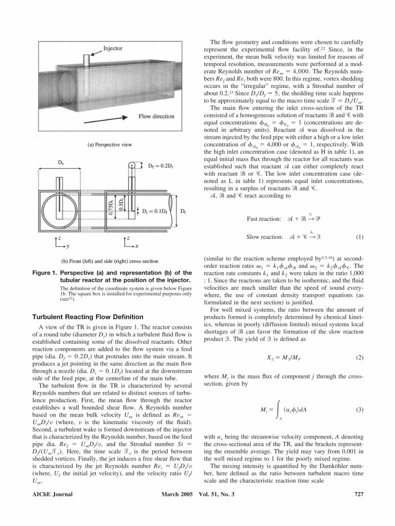
A view of the TR is given in Figure 1. The reactor consistsof a round tube (diameter Dt) in which a turbulent fluid flow isestablished containing some of the dissolved reactants. Otherreaction components are added to the flow system via a feedpipe (dia. Df � 0.2Dt) that protrudes into the main stream. Itproduces a jet pointing in the same direction as the main flowthrough a nozzle (dia. Di � 0.1Df) located at the downstreamside of the feed pipe, at the centerline of the main tube.

The turbulent flow in the TR is characterized by severalReynolds numbers that are related to distinct sources of turbu-lence production. First, the mean flow through the reactorestablishes a wall bounded shear flow. A Reynolds numberbased on the mean bulk velocity Um is defined as Rem �UmDt/v (where, v is the kinematic viscosity of the fluid).Second, a turbulent wake is formed downstream of the injectorthat is characterized by the Reynolds number, based on the feedpipe dia. Ref � UmDf/v, and the Strouhal number St �Df/(Um�v). Here, the time scale �v is the period betweenshedded vortices. Finally, the jet induces a free shear flow thatis characterized by the jet Reynolds number Rei � UfDi/v(where, Uf the initial jet velocity), and the velocity ratio Uf/Um.

The flow geometry and conditions were chosen to carefullyrepresent the experimental flow facility of.22 Since, in theexperiment, the mean bulk velocity was limited for reasons oftemporal resolution, measurements were performed at a mod-erate Reynolds number of Rem � 4,000. The Reynolds num-bers Ref and Rei both were 800. In this regime, vortex sheddingoccurs in the “irregular” regime, with a Strouhal number ofabout 0.2.23 Since Dt/Df � 5, the shedding time scale happensto be approximately equal to the macro time scale � � Dt/Um.

The main flow entering the inlet cross-section of the TRconsisted of a homogeneous solution of reactants � and � withequal concentrations ��0

� ��0� 1 (concentrations are de-

noted in arbitrary units). Reactant � was dissolved in thestream injected by the feed pipe with either a high or a low inletconcentration of ��0

� 4,000 or ��0� 1, respectively. With

the high inlet concentration case (denoted as H in table 1), anequal initial mass flux through the reactor for all reactants wasestablished such that reactant � can either completely reactwith reactant � or �. The low inlet concentration case (de-noted as L in table 1) represents equal inlet concentrations,resulting in a surplus of reactants � and �.

�, � and � react according to

Fast reaction: � � � ¡k1

�

Slow reaction: � � � ¡k2

� (1)

(similar to the reaction scheme employed by2,3,18) at second-order reaction rates �1 � k1�� and �2 � k2��. Thereaction rate constants k1 and k2 were taken in the ratio 1,000: 1. Since the reactions are taken to be isothermic, and the fluidvelocities are much smaller than the speed of sound every-where, the use of constant density transport equations (asformulated in the next section) is justified.

For well mixed systems, the ratio between the amount ofproducts formed is completely determined by chemical kinet-ics, whereas in poorly (diffusion limited) mixed systems localshortages of � can favor the formation of the slow reactionproduct �. The yield of � is defined as

X� � M�/MP (2)

where Mj is the mass flux of component j through the cross-section, given by

Mj � �A

�ux�j�dA (3)

with ux being the streamwise velocity component, A denotingthe cross-sectional area of the TR, and the brackets represent-ing the ensemble average. The yield may vary from 0.001 inthe well mixed regime to 1 for the poorly mixed regime.

The mixing intensity is quantified by the Damkohler num-ber, here defined as the ratio between turbulent macro timescale and the characteristic reaction time scale

Figure 1. Perspective (a) and representation (b) of thetubular reactor at the position of the injector.The definition of the coordinate system is given below Figure1b. The square box is installed for experimental purposes only(see22).


Da ��

�reaction(4)

For the reaction time scale we take �reaction �(k2

��0��0

)�1. By choosing different values for k1 and k2

(always in the ratio k1/k2 � 1,000:1), the Damkohler numberwas varied over eight orders of magnitude such that a verybroad spectrum of mixing regimes is covered. The fiveDamkohler numbers (indicated as case I–V) are listed in Table 1.

Numerical Simulation ProcedureTransport equations

The state at location x � xi (i � 1, 2, 3), and time t of anyturbulent reactive flow is defined by the local pressure p(x, t),velocity u(x, t) � ui, and scalar composition vector �(x, t) ��(x, t), where � � 1, 2, . . . , Ns refers to the Ns scalarcomponents involved in the set of reactions.10 For an incom-pressible, Newtonian fluid, the reacting scalar field is governedby the continuity equation, and the momentum and scalaradvection-diffusion equations

� � u � 0 (5)

�u�t

� u � �u � ��p � f � v�2u (6)

and

��

�t� u � �� J � �� (7)

where p is the pressure normalized with the mass density, f isa body force per unit mass acting on the fluid, v is the kinematicviscosity, J is the mass flux of the species given by Fick’s lawof diffusion J � Ji

� � ��/� xi (where � is the scalardiffusivity), and � � �� is the reaction rate that usually is anonlinear function of the local scalar composition array �(x).The second equation is generally referred to as the Navier-Stokes (NS) equation.

Large eddy simulation

Within the LES approach, a spatially and temporally invari-ant low-pass filter operator is applied to the Eqs. 5 and 6 inorder to remove the high-frequency fluctuations and, thus, to beable to obtain a numerically feasible solution on a computa-tional grid, coarser than the smallest fluid length scales. Thefilter operator (denoted as �. . .�L) introduces an additionalstress term (approximately �s � �uu�L � �u�L�u�L;24), whichrepresents the influence of the nonresolved subgrid scale (SGS)velocity fluctuations to the resolved velocity field.5 assumes an

eddy viscosity ve relating the SGS stress to the resolved strainrate according to �s � 2ve�S�L. The Smagorinsky eddy vis-cosity (denoted as ve,S), is related to the strain rate modulusS � �(2S2), and grid spacing � as ve,S � Cs

2�2S, where theSmagorinsky constant is a semi-empirical constant.

Although the Smagorinsky model is widely used, its short-comings are well recognized (for example,6,25). In the lowmesh Reynolds number limit (that is, when the dissipativescales are close to the grid size), the eddy viscosity in theconventional Smagorinsky model does not approach zero sincethe resolved strain rate remains finite. Therefore, we use amodified eddy viscosity proposed by6 according to

ve,V � ve,S � �v�1 � exp��ve,S

�v�� (8)

where � � 2/9 is recommended. The eddy viscosity given byEq. 8 correctly approaches zero in the low mesh Reynoldsnumber limit. On top of the Voke modification, also the vanDriest’s wall damping function26 is used, which suppresses theeddy viscosity in the wall boundary regions in order to take intoaccount the local reduction in length scales imposed by thewall.

Lattice-Boltzmann LES solver

An efficient solution algorithm for the NS differential equa-tions is provided by the Lattice Boltzmann (LB) solver.27,28 TheLB scheme is based on a very simple microscopic system offictitious particles that can hop between the sites of a regularlattice and may have collisions only on the lattice sites. Colli-sion rules are chosen such that on a macroscopic level thecontinuity and Navier-Stokes Eqs. 5 and 6 are recovered. Sincethe scheme is fully local in nature, it performs very efficientlyon parallel platforms; only communication between the adja-cent boundaries of neighboring domains is required.

An adaptive forcing technique7 is used to impose the flowboundary conditions. The technique describes the geometry bya set of M control points on the boundary lying inside theuniform, cubic LB grid. At the control points, a force isdynamically adjusted such that prescribed velocities are main-tained. At the tube and injector walls a zero slip velocity isimposed, while at the injection point a fixed velocity is set at asingle grid point located in the injector exit. In this way, amomentum point source rather than a well defined jet flow isimposed. We, hence, expect some resolution problems in thejet exit regions, although further downstream the resolutionrequirements are relaxed due to entrainment of ambient fluidfrom the main flow. Periodic boundary conditions are appliedin streamwise direction to sustain a developed turbulent flow atthe inlet. The length of the reactor tube was taken ten reactordiameters in order to ensure that the influence of the feed pipeat the inlet was minimal. This assumption will be checked in

Table 1. Damkohler Number 10log(Da) Corresponding to Five (I–V) Reaction Rates for TwoInlet Concentrations ��0

of Reactant �

Case I II III IV V

H ��0�4,000 �4.3 �2.3 �0.3 1.7 3.7

L ��0� 1 �4.1 �2.1 �0.1 1.9 3.9


the result section. The main flow is driven by a uniform bodyforce that is applied to the whole flow domain. The body forceis dynamically adjusted such that the momentum flow throughthe reactor is kept constant (which otherwise would increasedue to the jet).

Filtered density function

Just treating the scalar advection-diffusion Eq. 7 in the LEScontext (that is, on the analog of the SGS stresses) is notappropriate due to the lack of information about the jointdistribution of the reacting species on subgrid scale level,which is required to determine the filtered reaction rate � incase of second and higher order reactions.10 Rather, a transportequation for the joint probability density function of the LESfiltered scalar quantities (the filtered density function (FDF)) isformulated13,14

�PL

�t� �u�L � �PL � �� u��L � �u�LPL�

��

��Ji

�

�xi�

L

� ��PL� (9)

where �X�Y�L denotes the filtered value of X conditioned on Y,� is the value in composition space of the scalar quantity �,and the summation convention applies to both species suffix �and the coordinate suffix i. The FDF PL can formally bedefined as

PL�; x, t ��

�

�, �x�, tGx� � xdx� (10)

�, �x, t� � � � � �x, t� � ��1

Ns

� � � ��x, t� (11)

where � is the Dirac delta function, [�, �(x, t)] is known asthe fine-grained density29 and G(x) is the low-pass filter cor-responding to the LES filter operator �. . .�L.

An LES must be used to supply the resolved scale velocity�u�L. Equation 9 describes the change of the FDF PL due toseveral processes. The convection term (second term on thel.h.s.) and chemical reaction term (last term on r.h.s.) are closed(and, thus, do not need any modeling). The terms that needclosure are the unresolved SGS convection and diffusion term,given by the first and second term on the r.h.s., respectively.

An eddy viscosity model is adopted for the FDF SGS con-vective flux

�u��L � �u�L�PL � ��e�PL, (12)

where �e is the eddy scalar diffusivity related to the eddyviscosity through the turbulent Schmidt number: �e � ve/Sct.

The SGS diffusion term can be decomposed into a partwhich represents transport in physical space and a part whichrepresents transport in composition space

�

��Ji

�

� xi�

L

PL� � � � ��PL ��2

��2 ��LPL� (13)

where �� represents the scalar energy dissipa-tion rate of component �. The conditional scalar energy dissi-pation rate ��L takes care of the diffusion in compositionspace, and needs to be modeled. Note that the latter diffusionterm is negative, and therefore exhibits behavior opposite to thediffusion of a scalar quantity in physical domain; instead ofbeing smoothed, gradients in compositional domain are steep-ened toward a final equilibrium state of an impulse at the scalaraverage.

The “interaction by exchange with the mean” (IEM) model29

is a simple closure that assumes (originally referred to by29 as“least mean square estimation” (LMSE) model)

��2

��2 ��LPL� �

�

��

�m � � ��L�PL� (14)

Here, �m represents the frequency of mixing within the sub-grid, which is related to the subgrid diffusion coefficient andthe filter length

�m � C�� e/�G2 (15)

where C� � 3 (due to15).

Algorithm 0.1 Monte Carlo solution of FDFequation (16)

Read initial flow field u(x, t0)Read initial Monte Carlo particles (MCP) �(X�, t0)for n � 1, 2 . . . number of timesteps do

Update LES flow field �u(x), tn�L

Interpolate flow properties to MCPCalculate drift and diffusion at MCP (Eq. 20)Step MCP in physical space (eq. 17)Update ��(x, tn)�L from MCPCalculate scalar drift coefficient (eq. 21)Update MCP ��(X�, tn) (eq. 18)Deal with the boundary conditions

end

With the closures given by Eqs. 12 and 14 the modeled FDFtransport equation is

�PL

�t� �u�L � �PL � � � � � �e�PL�

��

��

�m� � ��LPL� ��

��

��PL� (16)

The closures used in this formulation are essentially the sameas15 used for the 2-D mixing layer.

FDF solver

The modeled FDF transport Eq. 16 gives a full statisticaldescription of the filtered scalar composition field. The firstmoment is equivalent to the equation that can be obtained by


low pass filtering the scalar advection-diffusion Eq. 7. In theFDF formulation, modeling of the reaction term is not requiredsince it remains closed.

A finite difference solution of FDF transport equation is notfeasible, since the computational demands grow exponentiallywith the dimension (that is, the number of species Ns) of thesystem. For high-dimensional systems, a Lagrangian MonteCarlo (MC) solver turns out to be more efficient.10 The idea ofthe MC method is to release computational particles randomlyinto the computational domain. Each particle represents thescalar composition �� at its current position X(t). The MCparticle position and composition are evolved according to thestochastic differential equations (SDE)

dX � DXt, tdt � EXt, tdWt (17)

and

d�� B��tdt (18)

where D and E are the drift and diffusion coefficients of theparticles in the physical domain, dW � dWi � (dt)1/ 2 i is aWiener process [with i a random variable with standardGaussian PDF];10, and B � B� denotes the drift in scalardomain due to micromixing and chemical reactions. The FDFtransport equation corresponding to the SDE Eq. 17 and Eq. 18is

�PL

�t� �� DPL �

1

2�2 E2PL� �

�

��

B�PL (19)

A comparison of this Fokker-Planck equation with the modeledFDF transport Eq. 16 shows that the two systems are equivalentfor a particular specification of the drift and diffusion coeffi-cients, viz

E � �2� � �e and D � �u�L � �� e (20)

respectively, and for the scalar drift coefficient

B � ��m�� L � ��t (21)

The solution procedure is given in algorithm 0.1. Linearinterpolation is used to obtain the flow properties at the MCP.The boundary conditions are set at the inflow of the main tubeand the jet. In order to attain a uniform particle density over thecross-section of the inlet to the reactor tube, every time step theboundary grid cells are filled with MC particles up to a pre-scribed particle density N0.

Practical aspects

The flow in the tubular reactor was calculated on a 800 �832 cubical computational grid with unity grid spacing �. Atthe wall of this domain, free slip boundary conditions wereimposed, except for the inlet and outlet, where periodic bound-ary conditions were taken. The outer tube wall had a diameterof 80�, and was defined by 220,635 control points, whereas thefeed pipe diameter of 16� was defined by 5,787 control points.

A circular hole in the feed pipe of 4� in diameter was defined.In the center of the hole, the jet flow was driven by a momen-tum source imposed on a single grid point.

The speed of sound in the LB framework is about one,implying that �u�2 �� 1 in order to keep the flow within theincompressible limit. The jet velocity was fixed at uj � 0.16(from here on, all quantities are specified in LB units) com-pared to 0.64 m/s in the physical equipment. The bulk flow wasdriven by a body force f0 that was dynamically adjusted via themass outflow in order to keep a fixed mean velocity (withoutthis adjustment, the bulk velocity would increase due to themomentum imparted by the jet). In this way, a mean velocityof 0.01 in the tube was established (compared to 0.04 m/s in thephysical equipment). A Reynolds number of 4,000 (which waschosen in agreement to the flow condition of the 3D-LIFexperiment of 22) was obtained by choosing a kinematic vis-cosity of v � 2.0 � 10�4. The LB solver requires to store 22(18 directions, 3 force components and one eddy viscosity)single-precision values on every grid node, resulting in a totalmemory requirement of approximately 0.45 GB.

The estimate of v combined with a molecular Schmidt num-ber of Sc � 2,000 leads to a molecular diffusivity of � �v/Sc � 1.0 � 10�7. The choice for the semi-empirical Sma-gorinsky constant was Cs � 0.12 (due to7). The turbulentSchmidt number relating the eddy diffusivity �e to the eddyviscosity ve was set to Sct � 0.7. This choice establishes adissipation of the nonresolved scalar fluctuations larger thanthe nonresolved velocity fluctuations. It was argued by,18 how-ever, that one single time scale relating the dissipation of bothspectra is probably not sufficient due to the distinct behavior ofthe high frequency part of the scalar power spectrum comparedto the kinetic energy power spectrum. This aspect will bediscussed in the results section.

The FDF solver is computationally more expensive than theLB-LES solver, and requires a larger amount of memory. Inorder to limit the computational effort of the reactive scalar,only the first half of the flow domain was employed; resultingin a 400 � 83 � 83 grid containing 20 Lagrangian MCparticles per grid cell on average. Each particle represented thefull composition array of the five scalar components of fiveindependent reaction schemes of varying Damkohler numbers(see table 1), so that in a single run several cases were calcu-lated. Every MC particle required 36 single-precision realvalues to be stored (25 for the reacting scalar components, onefor the nonreacting scalar, three for the position, three for thevelocity, one for the eddy viscosity, and three for the gradientvector of the eddy viscosity), resulting in a total memoryrequirement for the FDF solver of 400 � 832 � 20 � 36 � 4 �7.4 GB plus about 0.3 GB to store the Eulerian scalar field.

The code was implemented on a Linux cluster of ten dualAMD Athlon(TM) MP 1800� processors and one dual Pen-tium III 500 MHz processor with a total amount of 11 GB ofdistributed memory. The ten AMD processors took care ofFDF scalar solver, whereas the part of flow domain withoutscalars was solved on the slower Pentium III node. It tookabout 1.5 day to calculate one macro time scale Dt/Um (8000LB time steps). For an initial distribution, it took about a weekto obtain a steady flow, and the statistics were obtained fromabout 20 macro time scales (taking about a month for eachrun). For the simulations discussed in this article, the parallelcomputer cluster was kept busy for almost three months.


Results

Below, the results of the FDF simulation in the TR will bepresented. It has already been mentioned that within the FDFapproach the reaction term remains closed, and modeling ap-plies to the SGS mixing of the scalars only. Therefore, first ofall, the mixing of a nonreacting conserved scalar (denoted as�) replacing reactant � is studied and compared to the mea-surements described in the previous section. The mixing of thereactive scalars of the parallel competitive reaction systemdescribed earlier, will be presented next.

Conserved scalar mixing

First, some instantaneous results are presented to get quali-tative pictures of the flow, and the conserved scalar transport inthe TR. Next, a spectral analysis has been performed to gaininsight in the turbulent characteristics of the flow. Then, theaveraged conserved scalar concentration is compared to exper-imental 2D-LIF results. Finally, the performance of the FDF/LES model is assessed by comparing the concentration PDF’swith experimental LIF data.

Instantaneous Realizations. Impressions of the instanta-neous turbulent velocity field and the conserved (nonreacting),passive scalar concentration field are given in Figures 2 and 3,respectively. The velocity vector plot of Figure 2 shows that aturbulent wake is formed downstream of the injector. In thiswake, the jet at the exit of the injector is visible. In the verticalside view (Figure 2a), it is shown that the jet is inclinedupwardly promoted by the main stream flowing around theblockage formed by the feed pipe. Turbulent structures areformed and recirculation occurs. The yz-planes (coordinatedefinition in Figure 1b normal to the stream direction (Figure

2c–h) show the downstream development of the transversevelocity field.

The conserved scalar field shown in Figure 3 exhibits thesame features as a flow field: an upwardly inclined jet in aturbulent wake. The flow-normal yz-planes (Figure 3c–h) il-lustrate that the dye close to the feed pipe resides in the wake.The recirculation and low velocities in the wake of the injectorcause the dye to be distributed over the whole length of the feedpipe. This is most clearly visible in the flow-normal yz-plane(Figure 3c). The dye outside the wake is advected immediatelyaway due to the larger velocity of the main stream. Furtherdownstream, the dye is taken to the top of the reactor (fromposition p100 at x/Dt � 0.10), where it is directed along theouter wall of the tube. After position p300 (at x/Dt � 3.5), thedye reenters the central horizontal plane at both sides of thereactor.

For the flow around an infinitely long circular cylinder atRef � 800, vortex shedding occurs in the “irregular” regime,with vortices that become turbulent in themselves.23 In thetubular reactor the flow is more complex; the feed pipe cannotbe considered infinitely long, and a jet is injected into its wake.Even so, the horizontal cross-section view of the concentrationfield (Figure 3b) suggests that vortices at regular distances areformed in the tubular reactor. Earlier in this article, it wasestimated that in this particular flow geometry, the time �v

between the shedded vortices happens to be equal to the macrotime scale �. This implies that the distance between the suc-cessive vortices should be of the order of a reactor dia. Dt. Thisis roughly confirmed by the location of the vortices in Figure3b: the distance between two consecutive vortices (indicated byA and C) is about Dt.

Figure 2. Instantaneous velocity field in a vertical (a), and horizontal (b) center line plane, and six flow-normal verticalplanes (c–j) corresponding to the positions p020–p400.


Time Series and Spectral Analysis. Time series of thespanwise velocity component uy at three downstream positionsare shown in Figure 4. While the first position is at the injectoropening (Figure 4a), the second position is at x/Dt � 1.0 in the

wake close to the injector (Figure 4b), and the last position isat x/Dt � 7.6 far downstream (Figure 4c). The power spectraldensity functions corresponding to the time series are shown inFigure 5. The angular frequency is denoted as � � 2�/T,where T is the time. In the LB framework, the time resolution

Figure 3. Instantaneous conserved scalar field (same planes as Fig. 2).Labels A–C indicate shedded vortices. A log scale is used to pronounce the low scalar values with respect to the inlet concentration.

Figure 4. Time series captured at three downstreamcenter line positions x/Dt � 0.0 (a), x/Dt � 1.0(b) and x/Dt � 7.6 (c).The PDF’s are obtained from 25 macro time scales.

Figure 5. Normalized power spectral density functionscorresponding to the time series shown in Fig-ure 4.


is much higher than the space resolution.27 The highest fre-quency contribution in a time series is due to the advection ofthe smallest resolved spatial scale �x/Um. The angular fre-quency �RS corresponding to this time scale is used to nor-malize the frequency domain.

The transverse velocity fluctuations at the jet exit are sup-pressed. The power spectral density function falls off veryrapidly, and does not show any turbulent characteristics. In thewake (b) at x/Dt � 1, the turbulent fluctuations are mostintense (note the different vertical-scales of Figure 4a–c). Atthis position, the widest range of turbulent scales is found anda small inertial �5/3-range is recognized. At the far down-stream position x/Dt � 7.6, the fluctuation intensity is weakeragain, and the power spectral density hardly shows any inertialrange, which reflects the weak turbulence in a tube flow withRe � 4,000.

Although vortex shedding is found in the instantaneousconcentration field shown in Figure 3b, this is not visible in thepower spectral density function. It has already been mentionedthat vortex shedding was in the irregular regime, and, conse-quently, no truly fixed shedding periodicity is expected. On topof that, the Strouhal frequency of the feed pipe coincides withthe energy-rich turbulent macro time scales, which makes ithard to distinguish the energy contribution of the Strouhaloscillations to the power spectrum.

The time and spectral analysis shows that in spite of therelatively low Reynolds number Rem � 4,000, the flow ismoderately turbulent. Especially in the wake close to the feedpipe, an inertial range is formed and turbulence is generated. Atthe far downstream position, the low-mesh Reynolds numbermodification (Eq. 8) of the eddy viscosity model is required.

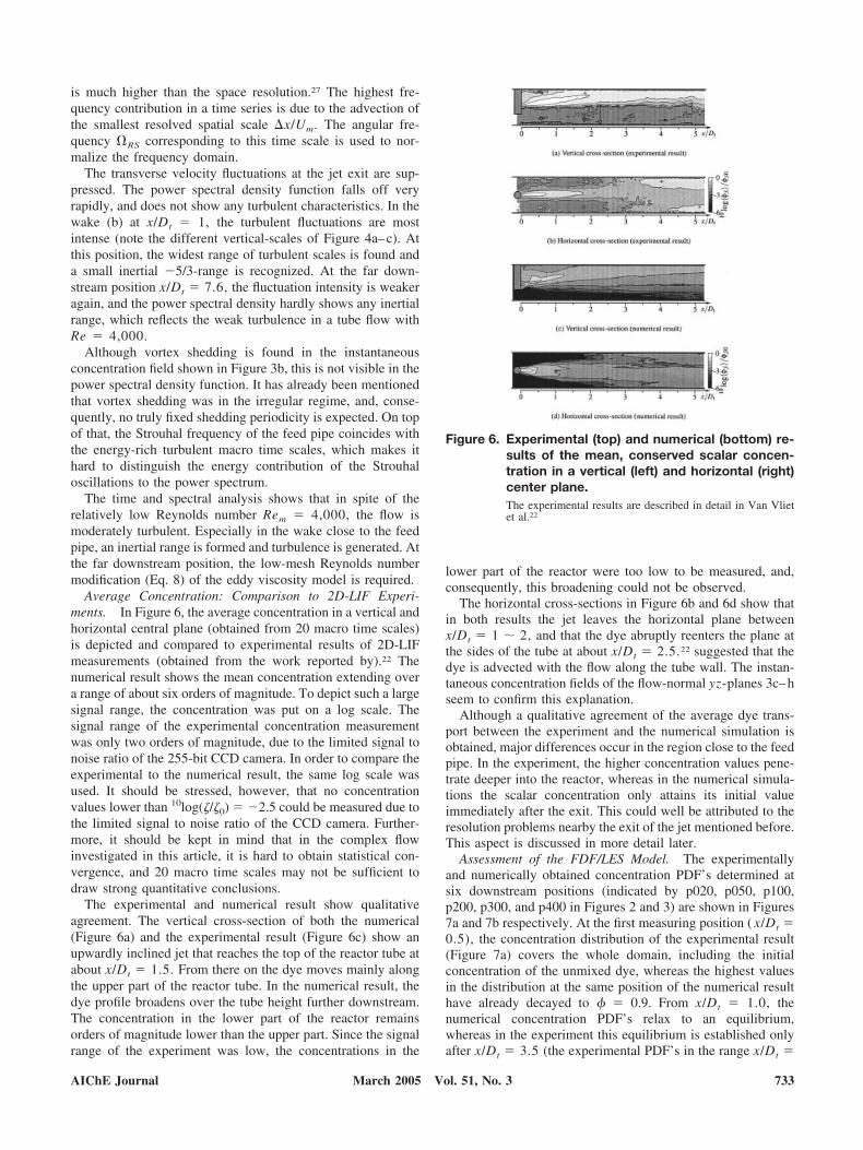
Average Concentration: Comparison to 2D-LIF Experi-ments. In Figure 6, the average concentration in a vertical andhorizontal central plane (obtained from 20 macro time scales)is depicted and compared to experimental results of 2D-LIFmeasurements (obtained from the work reported by).22 Thenumerical result shows the mean concentration extending overa range of about six orders of magnitude. To depict such a largesignal range, the concentration was put on a log scale. Thesignal range of the experimental concentration measurementwas only two orders of magnitude, due to the limited signal tonoise ratio of the 255-bit CCD camera. In order to compare theexperimental to the numerical result, the same log scale wasused. It should be stressed, however, that no concentrationvalues lower than 10log(�/�0) � �2.5 could be measured due tothe limited signal to noise ratio of the CCD camera. Further-more, it should be kept in mind that in the complex flowinvestigated in this article, it is hard to obtain statistical con-vergence, and 20 macro time scales may not be sufficient todraw strong quantitative conclusions.

The experimental and numerical result show qualitativeagreement. The vertical cross-section of both the numerical(Figure 6a) and the experimental result (Figure 6c) show anupwardly inclined jet that reaches the top of the reactor tube atabout x/Dt � 1.5. From there on the dye moves mainly alongthe upper part of the reactor tube. In the numerical result, thedye profile broadens over the tube height further downstream.The concentration in the lower part of the reactor remainsorders of magnitude lower than the upper part. Since the signalrange of the experiment was low, the concentrations in the

lower part of the reactor were too low to be measured, and,consequently, this broadening could not be observed.

The horizontal cross-sections in Figure 6b and 6d show thatin both results the jet leaves the horizontal plane betweenx/Dt � 1 � 2, and that the dye abruptly reenters the plane atthe sides of the tube at about x/Dt � 2.5.22 suggested that thedye is advected with the flow along the tube wall. The instan-taneous concentration fields of the flow-normal yz-planes 3c–hseem to confirm this explanation.

Although a qualitative agreement of the average dye trans-port between the experiment and the numerical simulation isobtained, major differences occur in the region close to the feedpipe. In the experiment, the higher concentration values pene-trate deeper into the reactor, whereas in the numerical simula-tions the scalar concentration only attains its initial valueimmediately after the exit. This could well be attributed to theresolution problems nearby the exit of the jet mentioned before.This aspect is discussed in more detail later.

Assessment of the FDF/LES Model. The experimentallyand numerically obtained concentration PDF’s determined atsix downstream positions (indicated by p020, p050, p100,p200, p300, and p400 in Figures 2 and 3) are shown in Figures7a and 7b respectively. At the first measuring position ( x/Dt �0.5), the concentration distribution of the experimental result(Figure 7a) covers the whole domain, including the initialconcentration of the unmixed dye, whereas the highest valuesin the distribution at the same position of the numerical resulthave already decayed to � � 0.9. From x/Dt � 1.0, thenumerical concentration PDF’s relax to an equilibrium,whereas in the experiment this equilibrium is established onlyafter x/Dt � 3.5 (the experimental PDF’s in the range x/Dt �

Figure 6. Experimental (top) and numerical (bottom) re-sults of the mean, conserved scalar concen-tration in a vertical (left) and horizontal (right)center plane.The experimental results are described in detail in Van Vlietet al.22


5.5 � 6.5 are not shown, but are more or less the same as thePDF at x/Dt � 4.5).

The mean and the variance obtained from the concentrationPDF’s are depicted in Figures 8a and 8b. The variance isnormalized with ��[1 � ��], that is, the upper bound varianceassociated to a completely segregated binary mixture (see forexample30). In Figure 8a, it is shown that the mean is under-predicted, consistent with the excessive spreading of the scalarmean as illustrated in the previous paragraph by Figure 6.Figure 8b shows that in the vicinity of the feed pipe (at x/Dt �0.0), the normalized variance is close to the upper bound ofone (that is, the mixture is almost completely segregated).Further downstream, the decreasing normalized varianceshows that micro mixing is becoming more and more active. Acomparison to the experimental results shown in the samegraph indicates that the FDF/LES model underpredicts thevariance in the first part of the reactor (up to x/Dt � 4),meaning that micro mixing in this region is overpredicted.Further downstream, after about x/Dt � 4, both the mean andthe variance predicted by the FDF/LES model are consistentwith the experiments.

The overprediction of the mean spreading of the scalar fieldmay be caused by an overprediction of either (1) the LESvelocity fluctuations or (2) the FDF SGS flux (due to thesecond term on the l.h.s., and the first term on r.h.s. of Eq. 9,respectively). In the vicinity of the jet exit, a transition regionexists of the laminar jet entraining into the turbulent wake of

the feed pipe. Such transition regions are not properly capturedby the Smagorinsky eddy viscosity model, since this modelassumes a local balance between production and small scaledissipation. In this particular region, the eddy viscosity is,therefore, likely to be overestimated, since the local reductionin length scales is not taken into account. Since an overesti-mated eddy viscosity contributes to the suppression of the LESvelocity fluctuations, we do not expect that mechanism (1) isresponsible for the excessive spreading of the jet. This assump-tion is consistent with the suppressed velocity fluctuations andthe non-developed turbulent power spectral density functionfound in the jet exit region, as was shown in figure 4. Mech-anism (2) (the FDF SGS flux), however, is proportional to theturbulent diffusivity (through the drift and diffusion in Eq. 20),promoting the turbulent diffusion length lt with respect tomolecular diffusion length l as lt/l � ��e/� � �(ve/v) ��(Sc/Sct). In our case, ve/v � 10 in the exit of the jet. On topof that, the assumed constant turbulent Schmidt number Sct �0.7 is adequate for a fully developed scalar spectrum only, andmay lead to overprediction of turbulent diffusivity in the vi-cinity of the scalar source (that is, in regions where the scalarspectrum has not developed yet) proportional to �Sc/Sct ��3,000. The inappropriate turbulence modeling in a laminarenvironment, hence, may lead to an overprediction of �e up totwo orders of magnitude, and likely is the cause of the exces-sive spreading of the jet via the overpredicted SGS flux.

Figure 7. Numerical and experimental downstream evo-lution of the concentration pdf of the nonre-acting scalar at positions x/Dt: 0.5 (bold); 1.0(solid); 1.5 (dashed); 2.5 (dotted); 3 (long dash-dot); 4.5 (short dash-dot).

Figure 8. The mean concentration, (a) and its variancenormalized with the upper bound variance��(1 � ��); (b) obtained from the concentra-tion pdf’s shown in Figure 7 against the dis-tance downstream the injector.


The overprediction of the mixing rate (observed as an ex-cessive decay of scalar variance in Figure 8b) may also be theresult of the overprediction of the turbulent diffusivity, leadingto an over prediction of the mixing frequency given by Eq. 15,and consequently, to an overprediction of scalar energy dissi-pation rate by the IEM micro mixing model (Eq. 14). Note thatthis overprediction is not a feature of the IEM model, but rathera result of an inaccurate estimate of the mixing frequency.

Some Concluding Remarks. So far, we have shown that themacro transport of a passive scalar is qualitatively reasonablywell predicted by the FDF/LES model: macro flow character-istics are recovered satisfactorily, and the distribution of thedye over the height of the reactor was consistent with experi-mental results. An overprediction of the decay of the scalarmean and variance in the vicinity of the injector was attributedto the over prediction of the turbulent diffusivity in the laminarto turbulent transition region of the jet, leading to an overpre-diction of the SGS flux. It was shown, however, that theseeffects were mainly confined to the first part of the reactor upto x/Dt � 3.5, and that from there on both experimental andnumerical results established a more or less similar equilibriumstate. We, therefore, expect that for simple reactions, the FDF/LES model used in the present research is adequate for cor-rectly predicting the selectivity.

Reactive scalar mixing

Now, the reactive system for several Damkohler numbersand two inlet concentrations (see table 1) is studied.

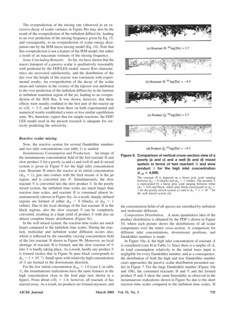
Instantaneous Consumption and Production. An image ofthe instantaneous concentration field of the fast reactant � andslow product � for a poorly (a and c) and well (b and d) mixedsystem is given in Figure 9 for the high inlet concentrationcase. Reactant � enters the reactor at its initial concentration(�� 1), gets into contact with the feed stream � in the jetregion, and is converted into �. Simultaneously, the slowreactant � is converted into the slow product �. In the poorlymixed system, the turbulent time scales are much larger thanreaction time scales, and reactant � is consumed almost in-stantaneously (shown in Figure 9a). As a result, sharply definedregions are formed of either �� 0 (black), or �� 1(white). Due to the local shortage of the fast reactant � in theblack regions, also the slow reactant � can be completelyconverted, resulting in a high yield of product � with also analmost complete binary distribution (Figure 9c).

In the well mixed system, the reaction time scales are muchlarger compared to the turbulent time scales. During the reac-tion, molecular and turbulent scalar diffusion occurs also,which is reflected by the smoothly varying concentration fieldof the fast reactant � shown in Figure 9b. Moreover, no localshortage of reactant � is formed, and the slow reaction of �into � is hardly taking place. As a result, hardly any product �is formed (notice that in Figure 9c pure black corresponds to�� 1 � 10�3). Small spots with relatively high concentrationof � are formed in the downstream direction.

For the low initial concentration ��0 � 1.0 (case L in table1), the instantaneous realizations have the same features as thehigh concentration close to the feed pipe (not shown in afigure). From about x/Dt � 1.0, however, all reactant � hasreacted away. As a result, no products are formed anymore, and

the concentration fields of all species are smoothed by turbulentand molecular diffusion.

Composition Distribution. A more quantitative idea of theproduct distribution is obtained by the PDF’s shown in Figure10, where each picture shows the distributions of all scalarcomponents over the entire cross-section. A comparison fordifferent inlet concentrations, downstream positions, andDamkohler numbers is made.

In Figure 10a–d, the high inlet concentration of reactant �is considered (case H in Table 1). Since there is a surplus of �,its total consumption relatively to the initial mass input isnegligible for every Damkohler number, and as a consequence,the distribution of both the high and low Damkohler numbercases approaches the passive scalar distribution presented ear-lier in Figure 7. For the large Damkohler number (Figure 10aand 10b), the consumed reactants � and � and the formedproduct � and � show the same bimodality as observed in theinstantaneous realizations shown in Figure 9a; due to the shortreaction time scales compared to the turbulent time scales, �

Figure 9. Comparison of vertical cross-section view of apoorly (a and c) and a well (b and d) mixedsystem in terms of fast reactant � and slowproduct � for the high inlet concentration��0 � 4,000.The reactant � is depicted on a linear gray scale rangingbetween �� 0 (black) and �B � 1 (white). The product �is represented by a linear gray scale ranging between white(�� 0.0) and black, where pure black corresponds to �� 1 for the poorly mixed system (c) and to �� 1 � 10�3 forthe well mixed system (d).


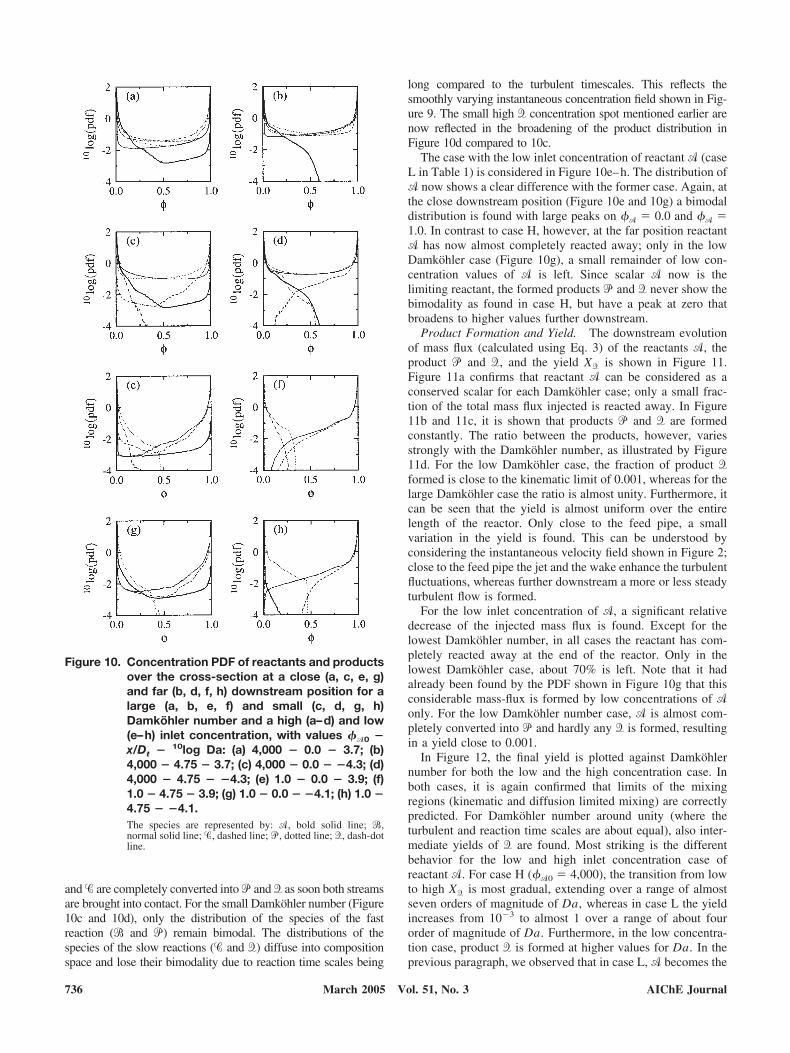
and � are completely converted into � and � as soon both streamsare brought into contact. For the small Damkohler number (Figure10c and 10d), only the distribution of the species of the fastreaction (� and �) remain bimodal. The distributions of thespecies of the slow reactions (� and �) diffuse into compositionspace and lose their bimodality due to reaction time scales being

long compared to the turbulent timescales. This reflects thesmoothly varying instantaneous concentration field shown in Fig-ure 9. The small high � concentration spot mentioned earlier arenow reflected in the broadening of the product distribution inFigure 10d compared to 10c.

The case with the low inlet concentration of reactant � (caseL in Table 1) is considered in Figure 10e–h. The distribution of� now shows a clear difference with the former case. Again, atthe close downstream position (Figure 10e and 10g) a bimodaldistribution is found with large peaks on �� 0.0 and �� 1.0. In contrast to case H, however, at the far position reactant� has now almost completely reacted away; only in the lowDamkohler case (Figure 10g), a small remainder of low con-centration values of � is left. Since scalar � now is thelimiting reactant, the formed products � and � never show thebimodality as found in case H, but have a peak at zero thatbroadens to higher values further downstream.

Product Formation and Yield. The downstream evolutionof mass flux (calculated using Eq. 3) of the reactants �, theproduct � and �, and the yield X� is shown in Figure 11.Figure 11a confirms that reactant � can be considered as aconserved scalar for each Damkohler case; only a small frac-tion of the total mass flux injected is reacted away. In Figure11b and 11c, it is shown that products � and � are formedconstantly. The ratio between the products, however, variesstrongly with the Damkohler number, as illustrated by Figure11d. For the low Damkohler case, the fraction of product �formed is close to the kinematic limit of 0.001, whereas for thelarge Damkohler case the ratio is almost unity. Furthermore, itcan be seen that the yield is almost uniform over the entirelength of the reactor. Only close to the feed pipe, a smallvariation in the yield is found. This can be understood byconsidering the instantaneous velocity field shown in Figure 2;close to the feed pipe the jet and the wake enhance the turbulentfluctuations, whereas further downstream a more or less steadyturbulent flow is formed.

For the low inlet concentration of �, a significant relativedecrease of the injected mass flux is found. Except for thelowest Damkohler number, in all cases the reactant has com-pletely reacted away at the end of the reactor. Only in thelowest Damkohler case, about 70% is left. Note that it hadalready been found by the PDF shown in Figure 10g that thisconsiderable mass-flux is formed by low concentrations of �only. For the low Damkohler number case, � is almost com-pletely converted into � and hardly any � is formed, resultingin a yield close to 0.001.

In Figure 12, the final yield is plotted against Damkohlernumber for both the low and the high concentration case. Inboth cases, it is again confirmed that limits of the mixingregions (kinematic and diffusion limited mixing) are correctlypredicted. For Damkohler number around unity (where theturbulent and reaction time scales are about equal), also inter-mediate yields of � are found. Most striking is the differentbehavior for the low and high inlet concentration case ofreactant �. For case H (��0 � 4,000), the transition from lowto high X� is most gradual, extending over a range of almostseven orders of magnitude of Da, whereas in case L the yieldincreases from 10�3 to almost 1 over a range of about fourorder of magnitude of Da. Furthermore, in the low concentra-tion case, product � is formed at higher values for Da. In theprevious paragraph, we observed that in case L, � becomes the

Figure 10. Concentration PDF of reactants and productsover the cross-section at a close (a, c, e, g)and far (b, d, f, h) downstream position for alarge (a, b, e, f) and small (c, d, g, h)Damkohler number and a high (a–d) and low(e–h) inlet concentration, with values ��0 �x/Dt � 10log Da: (a) 4,000 � 0.0 � 3.7; (b)4,000 � 4.75 � 3.7; (c) 4,000 � 0.0 � �4.3; (d)4,000 � 4.75 � �4.3; (e) 1.0 � 0.0 � 3.9; (f)1.0 � 4.75 � 3.9; (g) 1.0 � 0.0 � �4.1; (h) 1.0 �4.75 � �4.1.The species are represented by: �, bold solid line; �,normal solid line; �, dashed line; �, dotted line; �, dash-dotline.


limiting reactant. Although local shortages of � are formed, itwas found that this also leads to a shortage of �, and that, asa result, no product � can be created.

Discussion and Conclusions

In this article, we have presented one of the first attempts toapply the FDF/LES methodology to a turbulent reactive flow inan industrial geometry. More in particular, the mixing of re-acting scalars of a parallel competitive reaction scheme in atubular reactor was investigated. Although FDF/LES is com-

putationally very demanding (a parallel cluster of eleven dualprocessors has been kept busy for almost three months), thismodeling approach is attractive because of the minimum ofmodeling assumptions required due to the ability to keep thereaction term closed. Closures have to be adopted for thenonresolved SGS scalar transport terms in the FDF equation(the SGS convective flux and the SGS dissipation), which weremodeled by a gradient diffusion model (Eq. 12), and by theIEM model (Eq. 14), respectively.

The FDF closure models were assessed by means of exper-imental 2D-LIF data22 of the mixing of a fluorescent dye in theflow of the TR operated at the same process conditions. Theexperimental 2D-LIF measurements of the scalar distributionover a horizontal and vertical cross-section showed that theglobal macro transport of the conserved scalar was qualita-tively well predicted by the FDF numerical simulations; anonuniform distribution of the scalar dye over the height of thereactor was found due to the upwardly inclined jet promoted bythe blockage formed by the injector. Compared to the experi-mental results, however, the jet in the numerical simulationpenetrates somewhat less deep into the reactor. Both the decayof the scalar mean and scalar variance along the center line ofthe reactor were overpredicted in the in the vicinity of theinjector.

The findings above indicate that the FDF/LES simulationoverpredict the mean spreading of the jet, and the dissipation ofthe small scale fluctuations in the vicinity of the injector. Theseeffects were attributed to the overprediction of the turbulentdiffusivity in the transition region (where the laminar jet meetsthe turbulent wake of the feedpipe). Since the eddy viscositymodel employed in this research implicitly assumes fully de-veloped turbulence, it does not capture the local suppression ofsmall length scales in the laminar jet region. The resultingoverprediction of the turbulent diffusivity leads to an overpre-diction of the FDF SGS scalar flux (causing the excessivespread of the mean). Also, it leads to an overprediction of theFDF dissipation due to an overestimation of the mixing fre-quency (causing the excessive decay of scalar variance). Theproblems are noticeable in the direct vicinity of the jet exitonly, where the laminar jet emerges into the turbulent wake ofthe injector.

In spite of difficulties in jet region, it was shown that furtherdownstream, the predicted scalar mean and variance closelyagree with the experiments. Since the reactions mainly take

Figure 11. Downstream evolution of the total mass fluxof reactant �, the products � and �, and theyield X� for the high initial concentration of �(case H; fig. a–d) and the low initial concen-tration of � (case L; fig. e–h), shown for vary-ing logarithm of the Damkohler number cor-responding to cases defined in table 1: I ��4.3 (triangles); II � �2.3 (circles); III � �0.3(squares); IV � 1.7 (asterisks); V � 3.7(crosses).

Figure 12. Final yield vs. Damkohler number for low andhigh inlet concentration of �.


place in these regions, it is expected that the yield predictionsare not too much affected. The qualitative behavior of the yieldof the parallel competitive reactions indeed was well predicted,showing consistent physical behavior. The mixing limited andkinetic limited reaction were correctly predicted. The transitionbetween the regimes occurred around Da � 1.0 for the lowinlet concentration case, whereas in the high inlet concentrationcase the slow product � is formed two orders of magnitudesearlier due to the excess of reactant �. These observations maybe important in process design in finding an optimal mixingintensity for given inlet concentration and flow conditions.

For more complicated fast reactions (such as fuel combus-tion or polymer reactions) it may be more important to cor-rectly capture the scalar mixing in the vicinity of the jet. Inorder to take into account the local reduction of length scales,the use of dynamic subgrid scale models would be a betterchoice.31,32 Furthermore, as long as the scalar spectrum has notfully developed (such as in the vicinity of the injector), it is notlikely that a single turbulent Schmidt number is capable ofcorrectly relating the turbulent diffusivity to the eddy viscosityas in Eq. 12. Particularly, for inhomogeneous turbulent flows inindustrial process equipment, improved models have to beapplied. A good candidate is the spectral relaxation (SR)model,33 since it takes into account multiple time scales toexplicitly incorporate the shape and development of the scalarspectrum by construction. An alternative model including mul-tiple time scales is due to.34

In order to deal with the lack of intermittency and inabilityof the IEM model to modify the shape of the concentrationPDF, several improved micro-mixing models are available.The “particle interaction model,” the Langevin equation modeland the Fokker-Planck closure can be used to establish sto-chastic mixing in the composition domain.10,35 Drawbacks ofthe models, absence of relaxation to Gaussianity and unbound-edness of the scalar fields, respectively, are prevented by abinomial sampling model36 which combines the IEM and theparticle interaction model.

In conclusion, the FDF/LES approach yields very detailedinformation on turbulent reactive flows with the usage of aminimum of modeling assumptions. In spite of the diverse andcomplex mechanisms of turbulence generation making the TRflow representative of industrial flows, a fair agreement for theconserved scalar mixing is obtained, with consistent physicalbehavior for the interaction of the chemical kinetics and thecomplex hydrodynamics. Although the high computational de-mands make FDF simulations currently accessible to academicresearch only, the exponential growth of computer resourceswill make them a versatile tool for process and geometryoptimization of turbulent reactive flows in process industries.The primary focus should be on the development and incorpo-ration of more sophisticated closure models into the FDFequation.

Notation

A � cross-section surface of the tubular reactorB � scalar composition drift vector coefficientD � drift vector coefficient

Dt/Df/Di � diameter tubular reactor/feed pipe/injector holeDa � Damkohler number

E � diffusion coefficientJ � Ji

� � mass flux vector of specie �

Mj � streamwise mass flux of component jNs � number of species involved per reactionNp � number of Monte Carlo particles per grid cellPL � filtered density function

Rei � Reynolds number based on jetRef � Reynolds number based on feed pipe

Rem � Reynolds number based on mean flowS � resolved scale strain rate

Sc(t) � (Turbulent) Schmidt numberSt � Strouhal number

Um/Uf � mean velocity of main flow/jetW � Wiener process vectorX� � yield of the slow product �

f � body force vector per unit of massk1/k2 � fast/slow reaction rate constant

p � pressure per unit of massu � velocity vectorx � position vector

� � turbulent macro time scale�reaction � characteristic reaction time

� � index scalar component vector�/�e � molecular/eddy diffusivity

� � delta Dirac function � fine-grained density function

v/ve � kinematic/eddy viscosity�� variance of scalar fluctuations of ��s � turbulent shear stress� � composition vector� � scalar energy dissipation rate� � value of composition vector

�� reaction rate of component ��m � mixing frequency

DNS � direct numerical simulationFDF � filtered density functionIEM � interaction by exchange with the meanLES � large eddy simulationLIF � laser induced fluorescenceMC � Monte CarloNS � Navier-Stokes

PDF � probability density functionSED � scalar energy dissipationSGS � subgrid scale

SR � spectral relaxationTR � tubular reactor

Literature Cited1. Brethouwer, G., “Micro-Structure and Langrangian Statistics of the

Scalar Field with a Mean Gradient in Isotropic Turbulence,” J. FluidMech., 474, 193–255 (2003).

2. Bakker, R. A., and H. E. A. Van den Akker, “A Lagrangian Descrip-tion of Micromixing in a Stirred Tank Reactor Using 1D-MicromixingModels in a CFD Flow Field,” Chem. Eng. Sci., 51(11), 2643–2648(1996).

3. Baldyga, J., and J. R. Bourne, “A Fluid Mechanical Approach toTurbulent Mixing and Chemical Reaction Part II Micromixing in theLight of Turbulence Theory,” Chem. Eng. Commun., 28, 243–258(1984).

4. McMurtry, P. A., T. C. Gansauge, A. R. Kerstein, and S. K. Krueger,“Linear Eddy Simulations of Mixing in a Homogeneous TurbulentFlow,” Phys. Fluids A, 5(4), 1023–1034 (1993).

5. Smagorinsky, J., “General Circulation Experiments with the PrimitiveEquations: 1. The Basic Experiment,” Mon. Weather Rev., 91, 99(1963).

6. Voke, P. R., “Subgrid-Scale Modelling at Low Mesh Reynolds Num-ber,” Theoret. Comput. Fluid Dynamics, 8, 131–143 (1996).

7. Derksen, J. J., and H. E. A. Van den Akker, “Large Eddy Simulationson the Flow Driven by a Rushton Turbine,” AIChE J., 45(2), 209–221(1999).

8. Hollander, E. D., J. J. Derksen, and H. E. A. Van den Akker, “ANumerical Study on Othokinetic Agglomeration in Stirred Tanks,”AIChE J., 40(11), 2425–2440 (2001).

9. Ten Cate, A., J. J. Derksen, H. J. M. Kramer, G. M. Van Rosmalen,and H. E. A. Van den Akker, “The Microscopic Modelling of Hydro-


dynamics in Industrial Crystallisers,” Chem. Eng. Sci., 56, 2495–2509(2001).

10. Pope, S. B., “Pdf Methods for Turbulent Reactive Flows,” Prog.Energy Combust. Sci., 11, 119–192 (1985).

11. Steiner, H., and W. K. Bushe, “Large Eddy Simulation of a TurbulentReacting Jet with Conditional Source-Term Estimation,” Phys. Fluids,13(3), 754–769 (2001).

12. Wall, C., B. J. Boersema, and P. Moin, “An Evaluation of the AssumedBeta Probability Density Function Subgrid-Scale Model for LargeEddy Simulation of Nonpremixed, Turbulent Combustion with HeatRelease,” Phys. Fluids, 12(10), 2522–2529 (2000).

13. Pope, S. B., “Computations of Turbulent Combustion: Progress andChallenges,” Proc. Combust. Inst., 23, 591–612 (1990).

14. Gao, F., and E. E. O’Brien, “A Large Eddy-Simulation Scheme forTurbulent Reacting Flows,” Phys. Fluids A, 5, 1282 (1993).

15. Colucci, P. J., F. A. Jaberi, P. Givi, and S. B. Pope, “Filtered DensityFunction for Large Eddy Simulation of Turbulent Reacting Flows,”Phys. Fluids, 10(2), 499–515 (1998).

16. Zhou, X. Y., and J. C. F. Pereira, “Large Eddy Simulation (2D) of aReacting Plane Mixing Layer Using Filtered Density Function Clo-sure,” Flow, Turbulence and Combustion, 64, 279–300 (2000).

17. Jaberi, F. A., P. J. Colucci, S. James, P. Givi, and S. B. Pope, “FilteredMass Density Function for Large-Eddy Simulation of Turbulent Re-acting Flows,” J. Fluid Mech., 401, 85–121 (1999).

18. Van Vliet, E., J. J. Derksen, and H. E. A. Van den Akker, “Modellingof Parallel Competitive Reactions in Isotropic Homogeneous Turbu-lence Using a Filtered Density Function Approach for Large EddySimulations,” In Proc. of the 3rd Int. Symp. on Comp. Techn. forFluid/Thermal/Chemical Systems with Industrial Appl., Atlanta, GA(2001).

19. Cha, C. M., and P. Trouillet, “A Subgrid-Scale Mixing Model forLarge-Eddy Simulation of Turbulent Reacting Flows Using the Fil-tered Density Function,” Phys. Fluids, 15(6), 1496–1504 (2003).

20. Gicquel, L. Y. M., P. Givi, F. A. Jaberi, and S. B. Pope, “VelocityFiltered Density Function for Large Eddy Simulation of TurbulentFlows,” Phys. Fluids, 14(3), 1196–1213 (2002).

21. Sheikhi, M. R. H., T. G. Drozda, P. Givi, and S. B. Pope, “Velocity-Scalar Filtered Density Function for Large Eddy Simulation of Tur-bulent Flows,” Phys. Fluids, 15(8), 2321–2337 (2003).

22. Van Vliet, E., S. M. Van Bergen, J. J. Derksen, L. M. Portela, and

H. E. A. Van den Akker, “Time-Resolved, 3D, Laser-Induced Fluo-rescence Measurements of Fine-Structure Passive Scalar Mixing in aTubular Reactor,” Exp. in Fluids, 37, 1–21 (2004).

23. Williamson, C. H. K., “The Existence of Two Stages in the Transitionto Three-Dimensionality of a Cylinder Wake,” Phys. Fluids, 31(11),3165–3137 (1988).

24. Deardorff, J. W., “A Numerical Study of Three-Dimensional Turbu-lent Channel Flow at Large Reynolds Numbers,” J. Fluid Mech., 41,453–480 (1970).

25. Zang, T. A., and U. Piomelli, Large eddy simulation of transitionalflow, “Large Eddy Simulation of Complex Engineering and Geophysi-cal Flows,” B. Galperin and S. A. Orzag, eds., Cambridge UniversityPress,p. (1993).

26. Van Driest, E. R., “On Turbulent Flow Near a Wall,” J. Aero. Sci., 23,1007–1011 (1956).

27. Frisch, U., B. Hasslacher, and Y. Pomeau, “Lattice-Gas Automata forthe Navier-Stokes Equations,” Phys. Rev. Lett., 56(14), 1505 (1986).

28. Somers, J. A., “Direct Simulation of Fluid Flow with Cellular Autom-ata and the Lattice-Boltzmann Equation,” Appl. Sci. Res., 51, 127–133(1993).

29. O’Brien, E. E., “The Probability Density Function (pdf) Approach toReacting Turbulent Flows,” In: Topics in Applied Physics: TurbulentReacting Flows, P. A. Libby and F. A. Williams, eds., 44, 186–218(1980).

30. Fox, R. O., Computational Models for Turbulent Reacting Flows,Cambridge University Press, (2003).

31. Pope, S. B., Turbulent Flows, Cambridge University Press, (2000).32. Vreman, B., B. Geurts, and H. Kuerten, “Large-Eddy Simulation of

Turbulent Mixing Layer,” J. Fluid Mech., 339, 357 (1997).33. Fox, R. O., “The Lagrangian Spectral Relaxation Model of the Scalar

Dissipation in Homogeneous Turbulence,” Phys. Fluids, 9(8), (1997).34. Heinz, S., and D. Roekaerts, “Reynolds Number Effects on Mixing

and Reaction in a Turbulent Pipe Flow,” Chem. Eng. Science, 56,3197–3210 (2001).

35. Fox, R. O., “The Focker-Planck Closure for Turbulent MolecularMixing: Passive Scalars,” Phys. Fluids, 4(6), 1230–1244 (1992).

36. Valino, L., and C. Dopazo, “A Binomial Sampling Model for ScalarTurbulent Mixing,” Phys. Fluids A, 2(7), 1204–1212 (1990).

Manuscript received Aug. 26, 2003, and revision received July 9, 2004.


turbulent mixing in a tubular reactor: assessment of an...

Documents