MPRAMunich Personal RePEc Archive

Card versus cash: empirical evidence ofthe impact of payment card interchangefees on end users’ choice of paymentmethods

Guerino Ardizzi

Bank of Italy

29 May 2013

Online at https://mpra.ub.uni-muenchen.de/48088/MPRA Paper No. 48088, posted 8 July 2013 09:21 UTC

Journal of Financial Market Infrastructures 1(4), 73–105

Card versus cash: empirical evidence of theimpact of payment card interchange fees onend users’ choice of payment methods

Guerino ArdizziBank of Italy, Market and Payment System Oversight, Via Nazionale, 91 00184Rome, Italy; email: guerino.ardizzi@bancaditalia.it

(Received February 4, 2013; revised May 25, 2013; accepted May 29, 2013)

Interchange fees in card payments are a mechanism to balance costs and revenuesbetween banks for the joint provision of payment services. However, such feesrepresent a relevant input cost used as a reference price for the final fee chargedto the merchants, who may be reluctant to accept cards and induce the cardholderto withdraw cash. In this paper, we empirically verify for the first time the effectof the interchange fee on the decision to withdraw cash and compare it with thatof paying with payment cards, considering a balanced panel data set of Italianissuing banks. Finally, results show that there is a positive correlation betweenthe cash usage and the level of the interchange fees. Accordingly, regulation ofthe multilateral interchange fee level may be an effective tool in reducing cashpayments at the point of sale, although there is no clear evidence that a zerointerchange fee rate (or a close-to-zero rate) would be optimal.

1 INTRODUCTION

The objective of this study is to perform a first empirical investigation on the impactof the interchange fee on the propensity to use automated teller machine (ATM) cashwithdrawals versus card payments at the point of sale (POS). But first we have to takea step back and describe what interchange fees are and how they work the paymentnetworks, in which payment services are jointly provided by intermediaries to the ben-efit of different end users in a widespread network. In the leading credit and debit card

I wish to thank Lucia Bazzucchi, Daniele Condorelli, Federico Crudu, Massimo Doria, Paola Giucca,Eva St. Once an anonymous referee, and all seminar participants at the lunch seminar held at theBank of Italy (Rome, February 2013). The views expressed in this paper are those of the author anddo not involve the responsibility of the Bank of Italy.

73

74 G. Ardizzi

schemes, the merchant’s bank (the acquirer) pays an interbank exchange fee (inter-change fee) to the cardholder’s bank (the issuer) for each payment card transaction,in compensation for services received. These fees may cover very simple interbankservices or extremely complex ones (trademark, clearing, authorization, charge-back)that benefit different parties (banks, merchants and cardholders). Interchange fees areusually set multilaterally, that is, uniform fees (so-called multilateral interchange fees(MIFs)) are established by the governing bodies of the respective networks.

Moreover, heterogeneous types of customer in two-sided markets and networkindustries could justify the existence of interchange fee flows. In the case of paymentcard schemes, different own-price demand elasticities of cardholder and merchant canbe noted. For instance, whenever the interchange fee is directly transferred (or sur-charged) to the cardholder, network expansion could be hampered, as the cardholderwould not be willing to bear high expenses on payment card transactions.

The economic literature generally endorses the maintenance of an MIF, but showsthat, privately and socially, optimal interchange fees often diverge (Rochet and Tirole2002, 2011). In addition, the utility functions of the public authorities dealing withthe interchange fee problem are heterogeneous (Rochet 2007); for instance, competi-tion authorities may particularly care about end-user surplus, and central banks mayconsider the payment system as a whole.

Competition authorities claim that economic theory is not sufficient to justify anMIF, and the causal link between MIFs and efficiencies needs to be demonstratedempirically, since the interchange fee is a cost for the acquiring bank and may becomea de facto floor for merchant fees. Hence, setting a framework to determine whichMIFs can be justified on a case-by-case basis is one way of creating more effectivecompetition in payment card pricing.

After the adoption of the single currency in Europe, the issue of interchange feeshas also characterized the long and difficult process underway to create a single europayment area (SEPA). The European Commission recently launched a public dialogueon the present landscape of the cards network, including the possibility of regulatinginterchange fees (European Commission 2012).1 The Commission also conductedseveral legal assessments on the two major international card payment schemes (Visaand Mastercard).

The central banks, and the Eurosystem, in pursuit of its mandate to promote thesmooth operation of payment systems, generally claim that MIFs, if there are any,

1 For instance, as regards SEPA Direct Debit payment instruments (which allow bank customersto give companies or other organizations authorizations to take money directly from their bankaccounts to pay their bills in Europe) the European Commission has already issued an ad hocRegulation (924/2009) aimed to cap the MIF and to prohibit it after a transitional regime.

Journal of Financial Market Infrastructures 1(4), Summer 2013

Card versus cash 75

should not lead to bad price signals toward payers and payees, distracting them fromusing more efficient payment instruments (Börestam and Schmiedel 2011).2

More recently, economists have further analyzed the effect of interchange fees ontechnological innovation and on consumers’ choices of payment instruments, espe-cially considering the substitution between cash and payment card. The debate hasbeen directed toward the imposition of a “price cap” or “zero” MIF rule (Leinonen2011).

However, there are still few empirical studies on the issue of interchange fees,which has been mostly addressed by the literature from a theoretical point of view.For instance, to the best of our knowledge, available empirical evidence does notinclude direct estimates on the effect of the interchange fee on the choice of cash,which is considered inefficient in several studies on the social cost of retail paymentinstruments (Schmiedel et al 2012).

So we can return to the main objective of this study: assessing the impact of theinterchange fee on the propensity to use ATM cash versus card payments at the POS.Toward this aim, we consider a two-period balanced panel data set of about 300Italian issuing banks. The test is particularly interesting to perform in Italy, a countrycharacterized by a high propensity to use cash (Banca d’Italia 2012a).

In Section 2, we review the relevant literature on antitrust issues and the economicsof interchange fees. In Section 3 we give details and descriptive statistics on thepayment card market and the interchange fee both in Italy and the rest of Europe.Section 4 illustrates the model under analysis and the econometric approach. Theresults are discussed in Sections 5 and 6, while the conclusions and some policyindications are reported in Section 7.

2 ECONOMICS OF INTERCHANGE FEES

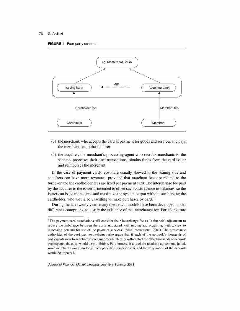
Interchange fees may be applied to any noncash retail payment network that involvesmore than one intermediary (such as checks, credit transfers, direct debits, etc). How-ever, they are most typical of the payment card schemes. The credit and debit cardnetworks are generally four-party schemes (Figure 1 on the next page), involving:

(1) the cardholder, who uses the card to purchase goods and services and generallypay an annual fee to the issuer;

(2) the issuer, the bank that issues the payment card to the cardholder;

2 In Italy, from 1998 to 2005, the Banca d’Italia (as the competition authority and overseer) estab-lished rules and requirements on the level of fees in Italy, and its approval was required after everyrevision. Since 2006, such rules have been adopted and updated by the general Antitrust Authority.

Research Paper www.risk.net/journal

76 G. Ardizzi

FIGURE 1 Four-party scheme.

Issuing bank Acquiring bankMIF

eg, Mastercard, VISA

Cardholder Merchant

Cardholder fee Merchant fee

(3) the merchant, who accepts the card as payment for goods and services and paysthe merchant fee to the acquirer;

(4) the acquirer, the merchant’s processing agent who recruits merchants to thescheme, processes their card transactions, obtains funds from the card issuerand reimburses the merchant.

In the case of payment cards, costs are usually skewed to the issuing side andacquirers can have more revenues, provided that merchant fees are related to theturnover and the cardholder fees are fixed per payment card. The interchange fee paidby the acquirer to the issuer is intended to offset such cost/revenue imbalances, so theissuer can issue more cards and maximize the system output without surcharging thecardholder, who would be unwilling to make purchases by card.3

During the last twenty years many theoretical models have been developed, underdifferent assumptions, to justify the existence of the interchange fee. For a long time

3 The payment card associations still consider their interchange fee as “a financial adjustment toreduce the imbalance between the costs associated with issuing and acquiring, with a view toincreasing demand for use of the payment services” (Visa International 2001). The governanceauthorities of the card payment schemes also argue that if each of the network’s thousands ofparticipants were to negotiate interchange fees bilaterally with each of the other thousands of networkparticipants, the costs would be prohibitive. Furthermore, if any of the resulting agreements failed,some merchants would no longer accept certain issuers’ cards, and the very notion of the networkwould be impaired.

Journal of Financial Market Infrastructures 1(4), Summer 2013

Card versus cash 77

there has been a general consensus (see Börestam and Schmiedel 2011) on the fact thatpayment card interchange fees may be useful in order to increase electronic payments.The two most frequently quoted articles on the economics of interchange fees areBaxter (1983) and Rochet and Tirole (2002). In his important early work, Baxter(1983) argues that under the assumption of perfect competition the socially optimalinterchange fee is generally nonzero, that internal forces will drive the interchange feeto the socially optimal level and that the authorities should not consider interchangefees in payment card networks negatively. Twenty years later, Tirole and Rochet(2002) analyzed the cooperative determination of the interchange fee and concludedthat raising the interchange fee will increase the use of credit cards so long as thefee does not exceed a level at which merchants no longer accept the card. A higherinterchange fee lowers cardholders’ fees, so that consumers who previously werenot cardholders are induced to become cardholders. The optimal interchange fee forissuers is the highest level at which merchants continue to accept the card, and it issignificantly different from zero.4

More recently, Rochet and Tirole (2003, 2011) have extended their analysis throughapplying the theory of the “two-sided market”, in which, under certain conditions (eg,different demand elasticities), one side of the market will pay relatively less than theother side, to take into account some positive indirect network externalities in themarket. In the payment card scheme, the side of the market that would pay relativelyless is that of the cardholder, since the issuing bank receives the interchange feerevenues from the acquiring bank. On the acquiring side, the merchant fee, whichincludes both the interchange fee input costs and the acquiring internal costs, will becharged to the merchant. This solution should allow the merchant to increase theirsales at the POS.5

4 Such an outcome is valid under the no-surcharge rule (issued by the self-regulatory bodies in ordernot to crowd out their payment cards), which prohibits affiliated merchants from charging higherprices to customers who pay with credit cards or from offering discounts to those who use otherpayment instruments, such as cash. Some economists claim that if such rules are removed (andsurcharges are allowed), the level of MIFs would not impact card usage (neutrality), as the cost andbenefit are transferred efficiently to the end users (Gans and King 2003; Zenger 2011). Nevertheless,retailers may be reluctant to surcharge (Jonker 2011; ITM 2000; European Commission 2010;Börestam and Schmiedel 2011). Moreover, in some countries, including Italy, surcharge to electronicpayments is prohibited by law in order to reduce the risk of promoting cash (see Coppola 2011;Doria 2010), as also pointed out by some empirical studies (Bolt et al 2008).5 In their contribution, Rochet and Tirole (2011) give a practical rule in order to internalize usageexternalities in two-sided payment card markets. This is known as the “tourist test”, or “merchantindifferent test” (MIT, as renamed by the competition authorities) and defines the optimal levelof interchange fees. As a result the “tourist test” understates the threshold interchange fee (andcorresponding merchant service commissions) at which a rational merchant would be indifferentbetween accepting cards or cash for a particular transaction.

Research Paper www.risk.net/journal

78 G. Ardizzi

With regards to the competition policy issues, antitrust authorities admit that MIFsare one way to internalize network externalities and thus to optimize card usage.However, MIFs also restrict competition and might be, therefore, prohibited to theextent that they do not generate sufficient efficiencies.6 In the more relevant antitrustdecisions (European Commission 2010), the European Commission has imposedcaps or some kind of audited self-regulation to reduce interchange fees over the year,under the assumption that such fees might undermine competition and inflate finalprices.

In this context, there is a common perception that on the acquiring side the merchantis charged according to an “interchange fee plus” model; accordingly, the merchantfee (mf) is calculated as follows:

mf D if C c C qc: (2.1)

In the notation of (2.1), “if” is the unit interchange fee, c represents the direct unitinternal cost for the acquirer and q is the margin in proportion to the direct costs tocover indirect costs together with the profit. The antitrust authorities fear that such apricing mechanism sets a de facto floor limit on the price that merchants must payto the acquirer for accepting payment cards. We consider such an assumption in ourempirical model of analysis in Section 4.

The next step in the literature is then to relate the MIF with a bias toward the useof cash. A recent discussion paper published by the Bank of Finland (Leinonen 2011)has focused on the problem of the MIF and the “cash cross-subsidies” on the issuingside. According to Leinonen, “the higher the MIF, the larger the cross-subsidy forcash”, provided that interchange fees increase payment costs for the merchants, whobecome reluctant to accept cards instead of cash, and thus reduce the possibility ofpassing on to customers the cost savings resulting from card efficiency.

Unfortunately, there is a scarcity of empirical contributions evaluating the effectsin the real world of the interchange fee mechanism, due to the lack of reliable dataon this matter. From the available studies in Europe, a decreasing trend in differentEuropean countries is associated with an increased usage of cards and competitionbetween card schemes (Börestam and Schmiedel 2011; Bolt and Schmiedel 2013).Chakravorti et al (2009) analyze the positive effect on the growth of payment cardtransactions after the interchange fee regulation in Spain (ceilings on the MIF levels).

6 The multilateral setting of the interchange fee among participants of a payment scheme, evenwhere it is a default level with the possibility to negotiate a lower fee on a bilateral basis, mayconstitute a restriction of market competition pursuant to antitrust legislation. In allowing such amultilateral agreement, the antitrust authority must determine whether setting a multilateral fee “mayimprove the supply of payment services since banks avoid a large number of bilateral negotiationsand transaction costs are reduced”, with potential benefits for the final customer (Bank of Italy,Provision 23, October 8, 1998).

Journal of Financial Market Infrastructures 1(4), Summer 2013

Card versus cash 79

FIGURE 2 Cash card ratio and payment cards transactions.

0

2

6

8

10

12

0 10 20 30 40

4

50 7060 80 90

Denmark Sweden

Netherlands Belgium

UK

Luxembourg France FinlandPortugal

AustriaEU

Euro area

Estonia

Germany

Latvia

PolandSlovakia

Slovenia

Hungary LithuaniaCzechRep. Romania

BulgariaGreece

IrelandSpain

ItalyMalta

Cyprus

Tra

nsac

tions

per

PO

S (

thou

sand

s)

Cash–card ratio (%)

Data for card payments per POS in 2011. Sources: European Central Bank, Blue Book statistics.

Nevertheless, the aforementioned authors test the impact of the interchange fee capregulation on the merchant acceptance of cards in Spain but the issue of the impact ofthe interchange fee on the cardholder’s inclination to shift to cash remains unsettled(Börestam and Schmiedel 2011).

Therefore, we shall test empirically the cash demand in relation to the interchangefee in Italy, after a brief description of the payment card landscape.

3 PAYMENT CARD MARKET,THE CARDHOLDERS’ PROPENSITYTO USE CASH AND THE INTERCHANGE FEE

The payment card is the most prevalent noncash instrument in Europe. Card transac-tions accounted for 40% of cashless payments in 2010, and volumes are increasingat around 6–7% per year (European Central Bank statistics 2012). In Italy there wereover 1.5 billion annual payment card operations in 2010, representing 38% of thetotal noncash payments that year (compared with 21% in 2000), but the “gap” withother industrialized countries is still large: only twenty-seven card transactions percapita annually compared with over seventy in the whole EU in 2010 (Banca d’Italia2012b).

Research Paper www.risk.net/journal

80 G. Ardizzi

FIGURE 3 MIF and cash–card ratio.

DenmarkSweden

NetherlandsBelgium

UK

Luxembourg

France

Finland

Portugal

Austria

Estonia

Germany

Latvia

Poland

Slovakia

Slovenia

Hungary

Lithuania

CzechRomania

Bulgaria

Greece

Ireland

Spain

ItalyMalta

Cyprus

0 20 40 60 80 100

0

0.2

0.4

0.6

0.8

1.0

1.2

1.4

1.6

1.8

Cash–card ratio (%)

MIF

leve

l (%

)

Sources: European Central Bank, Visa EU, Mastercard.

The latest data confirms that cash is still the most widely prevalent payment instru-ment in Italy, to a greater extent than in other industrialized countries (over 90% oftransactions at the POS, compared to around 80% in the rest of Europe (see Schmiedelet al 2012)). This is also confirmed by comparing the cash–card ratio per country.The cash–card ratio gives the value of cash acquired from ATMs divided by the totalvalue of card turnover (the total value ofATM withdrawals plus the total value of debitPOS expenditure by card (see Jones and Jones 2006)). In Figure 2 on the precedingpage, the cash–card ratio per country is plotted in relation to the number of domesticcard payments divided by the number of POSs: it is obviously a negative correlation,and Italy is on the side of the chart (the axes are centred on the mean values of thedistribution) with countries that present a low level of POS utilization and a highpropensity to use a card to acquire cash.

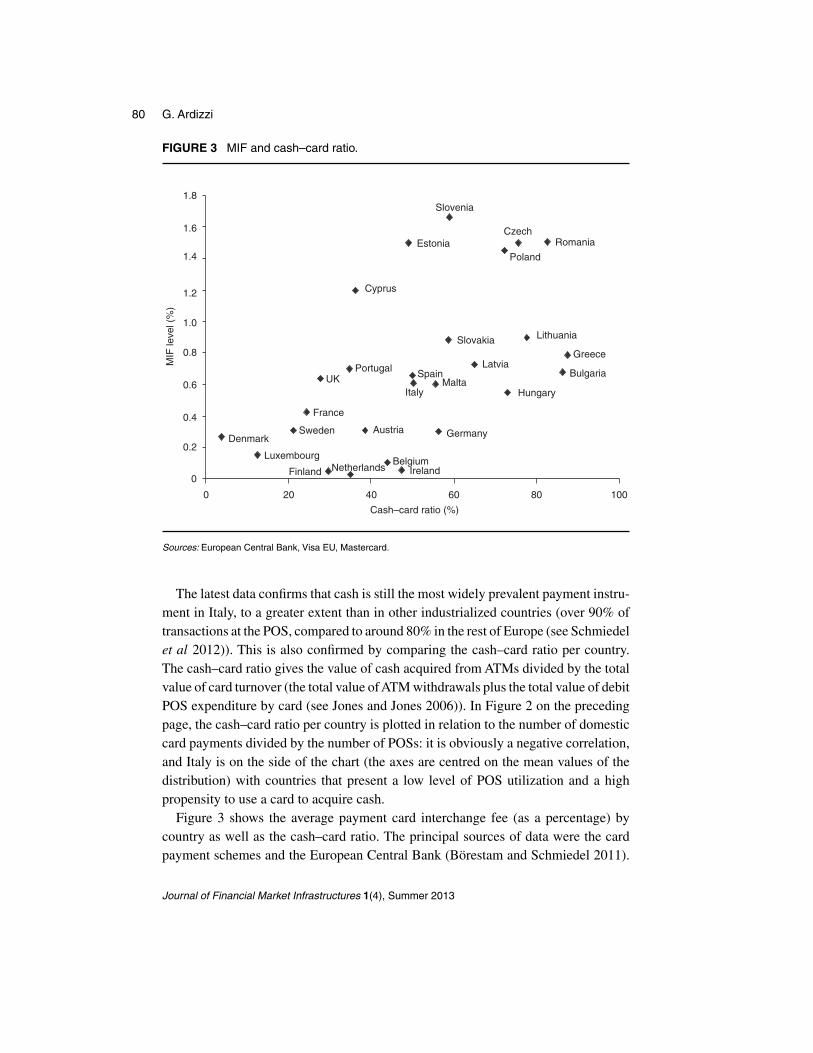
Figure 3 shows the average payment card interchange fee (as a percentage) bycountry as well as the cash–card ratio. The principal sources of data were the cardpayment schemes and the European Central Bank (Börestam and Schmiedel 2011).

Journal of Financial Market Infrastructures 1(4), Summer 2013

Card versus cash 81

There is a positive correlation between the use of debit cards at ATMs and interchangefee levels: in those countries where the interchange fee is the lowest, debit cards seemto be more widely used and accepted at the POS. Moreover, there is a significantvariability between average levels of the MIF (on the horizontal axis): the average(transaction-weighted) MIF varies from a minimum of about 0.01% to over 1.55% indifferent member states (Börestam and Schmiedel 2011).

4 MODEL OF ANALYSIS

The model of analysis is based on the functioning of a payment card on the issuingside (Leinonen 2011): banks or other payment service providers issue payment cardsin order to allow the cardholders to charge purchases or withdraw cash directly againstfunds on a transaction account at a deposit-taking institution (debit cards), prepaidaccount (prepaid cards) or according to credit facilities (credit cards). Payment cards(especially debit cards) may be used for ATM transactions as well as at POS terminalsat retail locations.7 When the payment card is used directly in shops, the issuer receivesinterchange fees revenues from the acquirers in the case of “not on us” transaction(when the issuer and the acquirer are not the same party). If the issuer and the acquirerare the same party (an “on us” transaction), the interchange fees are not applied butremain an implicit acquiring cost element in the pricing to the merchant. In everycase, the cardholder does not usually pay variable fees at the POS.

When the card is used in the ATM card networks, the cardholder is charged a feeonly if the transaction is performed at a “foreign ATM” (owned by an institutiondifferent from the issuing bank), because in the case of “foreign transactions” theissuer will pay an interbank service fee to the ATM owner. Nevertheless, in the caseof cash withdrawals at the issuer’s ATM, transactions are usually free of charge forcardholders. In fact, over 75% of ATM transactions are carried out at issuer’s ATMterminals in Italy (Ardizzi and Coppola 2002).

In this work we jointly consider all types of cards (debit, credit, prepaid) for avariety of reasons. First of all, in this way we can remain aloof of any substitutioneffects between cards. Second, many merchants agree on a product bundle which isoffered at a “blended” price that makes it difficult to compare different card types costof acceptance (European Central Bank 2006). Finally, available revenue informationon the cardholder is not always easily distinguishable between types of cards. For thisreason, debit card networks usually show lower interchange fees than credit cards(European Commission 2010), and issuing banks specializing in credit cards receivehigher average levels of interchange fee.

7 However, in this work we consider all the payment card types (debit, credit, prepaid) issuedby banks, so as to control for any substitution effect among cards and because of difficulties indistinguishing statistical information.

Research Paper www.risk.net/journal

82 G. Ardizzi

FIGURE 4 Transmission channel of the interchange fee mechanism.

Issuing bank

Interchange fee

Merchant fee

Cardholderaction

Merchantchoice

Cash–card ratio

POS andATM transactions

Issued customer card

On the issuing side we can correlate the POS interchange fee and the behavior of thecardholder interacting with the merchant. Given the “interchange fee plus” mechanism(Section 3), if interchange fees are too high, merchants might be reluctant to acceptthe card at the POS and induce the cardholder to shift to cash. Figure 4 illustrates themain transmission channels of the interchange fee mechanism on the issued customercard according to our model analysis.

This approach has the advantage that it does not require a simultaneous equationmodel (as in Chakravorti et al 2009 or Bolt et al 2008), which may impose severalrestrictions. We focus on the final information collected by the card-issuing bank,overcoming the problem of modeling the interaction between the merchant and thecardholder: the result of this interaction is given by the value of cash withdrawn andof POS payments carried out through the same cards, on which the issuer gains theinterchange fee from the acquirer.8

8 On the other hand, the acquiring bank does not collect information on the cash withdrawals withthe same cards. Moreover, reliable information on the acquiring side is not available. For thesereasons we do not consider a simultaneous equation model as in Chakravorti et al (2009).

Journal of Financial Market Infrastructures 1(4), Summer 2013

Card versus cash 83

Moreover, our model is valid even when merchants want (or are allowed) to applya surcharge on card payments: if the interchange increases average unit transactioncosts, a merchant will be less inclined to accept card payments or will be more likelyto surcharge card payments (Jonker 2011; Bolt et al 2010) with the same effect: toinduce the cardholder to withdraw cash at the ATM.

We can then assume a linear relationship between the cash–card ratio, theMIF and other control variables Z, with conditionally independent errors E."it jZit ;MIFit / D 0, i banks and t periods, and run a regression model such as thefollowing:

cash ratioit D ˛0 C a1MIFit CX

h

˛hZit C uit : (4.1)

The dependent variable (cash ratio) is equal to the ratio of ATM cash withdrawals tothe total amount of card turnover (at POS and ATM), which is consistent with the“cash–card ratio” described in Section 3.9

The first variable on the right-hand side of (4.1) is equal to the percentage of theaverage transaction-weighted (Chakravorti et al 2009) MIF received by the issueron its cards. Its coefficient aims to capture the effect of the interchange fee on thecash–card ratio of the same cards issued by the bank.10 To identify this effect, wefollow a two-stage process. In the first stage we assume, as usual, linearity in thefunctional relationship. In this case, it is essential that we have linearity in the MIFparameter, but not necessarily essential in the predictor. Accordingly, in this sectionwe shall determine the existence of a trend of the MIF impact with respect to thecash–card ratio in Italy. In other words, we verify whether an increase in the level ofthe MIF gives rise, on average, to more ATM cash withdrawals than card paymentsat the POS.

Thus, we put forward our first hypothesis:

(H0) under condition of linearity in the parameter, the higher the interchange fee,the higher the cash–card ratio on the issuing side, and vice versa.

In Section 6, as a second stage of the analysis, the linearity assumption will be removedin order to further investigate the issue “what about the optimal MIF?” Economic

9 In this case, we did not include theATM operations in the denominator so as to avoid the dependentvariable being truncated between zero and one.10 Although the interchange fee levels are usually set by a self-regulatory body, various marketconditions will, of course, affect the MIF variability at the level of the banks. This variabilityis remarkable and supposedly exogenous with respect to the payments and withdrawals of cashthrough ATMs. In other words, even if the selection of the card at the POS automatically affects theMIF received by the bank in our model, we are most interested in assessing how the variability ofthe interchange fee level affects the cash usage. Accordingly, self-selection problems related to thechoice of the debit and credit cards may be omitted in our model.

Research Paper www.risk.net/journal

84 G. Ardizzi

theory (Rochet and Tirole 2002) affirms that interchange fees may increase the cardusage at the POSs (accordingly, the cash ratio tends to decrease11) up to a threshold/optimal level, after which the acceptance costs surpass the benefit, the shift (return)to cash becomes relevant and the cash ratio rises. However, adding nonlinearity (or“second-order” effects) in the econometric model may be complex and requires furtherstatistical checks; we focus on this issue in the next section.

The summation term among the covariates in (4.1) indicates the set of h envi-ronmental variables (Z), and that of the relative coefficients, which can influencethe use of cash versus electronic payments at the POS. Control variables identifyincome components, which are also highly correlated with financial literacy, leadingto less use of cash, and access point diffusion (ATMs, bank branches, POSs), whichmay affect the choice between cash and alternative payment instruments (Stix 2004;Humphrey et al 1996).

One of the control variables identifies the individual income component, which isalso highly correlated with general education and financial literacy, leading to lessuse of cash and greater confidence in alternative payment instruments (Stix 2004;Humphrey et al 1996). In the model, such an income component is indirectly measuredby the value of total turnover per card for transactions that are completed at POSsand ATMs.12 Therefore, we considerZ1 D turnover. Even the expected effect of thisvariable on the cash–card ratio is positive, and the related hypothesis to be tested isthe following:

(H1) the higher the average turnover per card, the lower the inclination toward theuse of cash withdrawals as an alternative to electronic card payments.

A second control variable (Z2 D ATM) takes into account the relative size ofthe ATM card network managed by intermediaries, expressed as the ratio of thenumber of own ATMs and the number of own POSs.13 A larger diffusion of the ATMcard network may increase the probability of the bank having its own ATM cashwithdrawals, which are free of charge for the cardholder (positive coefficient). Wethen formulate the following hypothesis:

11 Actually, to the best of our knowledge the net impact on the cash–card ratio is not clearly inves-tigated by the theoretical models.12 The turnover per card represents a proxy of the spending capacity of the cardholders, as we donot dispose of detailed information on the effective average income per cardholder.13 The latter standardization allows us to compare issuing banks characterized by different businessstrategies:ATM services versus POS or acquiring services.At this stage, we do not include separatelythe number of POSs in the equation, as the correlation between the number of ATMs and POSs isvery high (0:82), increasing the risk of collinearity in the model. However, as a further test of stabilitywe also include separately ATM (expected sign: positive) and POS (expected sign: negative) (seeSection 5.3).

Journal of Financial Market Infrastructures 1(4), Summer 2013

Card versus cash 85

(H2) the bigger the ATM network, the higher the motivation toward the use of cashwithdrawals as an alternative to electronic card payments.

Moreover, in order to control the over-the-counter (OTC) cash operations that couldcrowd out ATM cash withdrawals, our model includes an indicator of the relativeincidence of the number of physical bank branches (OTC) to the number of automatedcash machines or ATM (Z3 D OTC). This control variable is expected to affect thecash–card ratio negatively, according to the following hypothesis:14

(H3) the higher the diffusion of the OTC network (number of branches to ATMs),the lower the motivation toward the use of cards to withdraw cash at ATMs.

As in the works of Chakravorti et al (2009) and Bolt et al (2008), we will notinclude the rate of interest in the model analysis: based on standard economic theory,the interest rate is expected to have a negative effect on the demand for money, via itsrole of opportunity cost of holding cash in alternatives to interest-bearing assets.15

However, since we want to further test the stability of our outcomes, in the robust-ness analysis we also include among the covariates a proxy of the interest rate levelscalculated as the ratio of the total amount of interest expenses to the total amount ofdeposit liabilities (data is available for all the banks in the panel).

Finally, in the longitudinal models the term uit in (4.1) can be broken down intoan individual specific effect, a temporal effect and the stochastic disturbance ("it ). Inparticular, the individual specific effect incorporates the unobservable elements16 of“firm-specific” or “group-specific” heterogeneity, reducing the omitted variable bias

14 As a further test of stability of the empirical results, we remove such a hypothesis from theequation model in Section 5.3 (“robustness”), by assuming that the effect of demand for OTC cashwithdrawals is neutral for the dependent variable and homogenously affects both ATM (negatively)and POS (negatively) transactions.15 One reason to omit the interest rate at this first stage is that available banking data on interest ratesis not consistent, as it does not consider only the cardholders’ current accounts and does not fullymatch that on our balanced panel database. Moreover, the inclusion of the deposit interest rate mayhamper the endogeneity problems, since it may be simultaneously affected with other variables (ie,size and institutional ones). Furthermore, several studies investigating the role of innovative paymentsystems in cash demand of Italian households (Lippi and Secchi 2009; Alvarez and Lippi 2009)point out that the progress in transaction technology may substantially reduce (or even eliminate)the impact of the interest rate on the cash demand of buyers, also considering that the period coveredby our estimations was characterized by very low interest rates, which are likely to have stronglymitigated the speculative motive. Finally, our model deals with a ratio of cash-to-card paymentflows rather than stocks of liquid assets, which implies the effect of the interest rate is ambiguous,which could in principle impact proportionally on both denominator and numerator of the ratio,leading to null overall effect.16 These elements may, for example, be linked to the internal payment procedures, to the type ofcustomer and to the differences in the business strategies.

Research Paper www.risk.net/journal

86 G. Ardizzi

TABLE 1 Panel data set. [Continues on next page.]

(a) Definition of variables and data sources

Variable Definition Source

MIF Average transaction-weighted interchangefee received by the issuing bank

BoI banking statisticsand survey on thecost of paymentinstruments

Cash ratio Ratio of the value of total ATM cashwithdrawals accounts to the value of totalPOS payments with issued debit and creditcards

BoI banking statistics

ATM Ratio of the number of owned ATMs tonumber of owned POSs by the issuingbank

BoI banking statistics

OTC Ratio of the number of bank branches tothe number of ATMs

BoI banking statistics

Turnover Total value of card operations to totalnumber of issued cards

BoI banking statistics

I rate Ratio of the total amount of interest ondeposit to the total value of bank deposits

BoI banking statistics

(b) Descriptive statistics

Variable Mean SD Min Max Obs

MIF overall 0.007 0.005 0.000 0.026 N D 546between 0.004 0.000 0.023 n D 273within 0.002 �0.004 0.018 T D 2

Cash–card overall 1.879 1.509 0.685 11.468 N D 546ratio between 1.492 0.860 8.593 n D 273

within 1.104 1.031 3.424 T D 2

ATM overall 0.043 1.724 0.006 0.534 N D 546between 1.708 0.007 0.247 n D 273within 1.109 0.020 0.093 T D 2

Turnover overall 1383.879 1.265 493.454 2915.985 N D 546between 1.245 727.352 2453.721 n D 273within 1.090 846.756 2261.716 T D 2

OTC overall 0.921 1.357 0.333 3.000 N D 546between 1.348 0.412 2.500 n D 273within 1.067 0.582 1.456 T D 2

Journal of Financial Market Infrastructures 1(4), Summer 2013

Card versus cash 87

TABLE 1 Continued.

(c) Correlation matrix

Variable Cash ratio MIF Turnover ATM OTC

Cash ratio 1.0000MIF 0.3928 1Turnover �0.1787 �0.0089 1ATM 0.0778 �0.0038 0.0702 1OTC �0.1789 �0.1108 �0.1308 �0.0691 1

in the estimates. We do not formulate the hypothesis here. The time-specific effect canbe captured by providing a time dummy variable, which may be useful for consideringthe effects of business cycle influences or technological changes (Chakravorti et al2009).

5 ESTIMATION OF THE LINEAR SINGLE EQUATION MODEL

5.1 Data set and estimation methodology

We use bank data drawn from the reports of the intermediaries on payment servicescollected by Banca d’Italia and from the survey on the costs of retail payments inItaly conducted in 2010 in close cooperation with the European System of CentralBanks (Schmiedel et al 2012; Banca d’Italia 2012a). Combining the different sourcesof information, on the basis of the available data (accumulated at the bank level) ithas been possible to construct a biannual (2009–2010) balanced panel of 273 issuingbanks representing about 60% of the debit and credit card market in Italy. The databasecontains data (counted from the side of the issuing bank for 2009) concerning theinterchange fee levels, cash and POS transactions, cards and accepting terminals,branches and other firm-specific variables. Table 1 on the facing page reports thedefinition, descriptive statistics and information about the different data sources forthe whole sample.

As has been noted in the theoretical literature (Zenger 2011), payment networkstypically differentiate their interchange fees by setting a variety of sector-specificMIFs for the same payment card. Figure 5 on the next page shows the density functionof the average (transaction-weighted) percentage interchange fee for issuing banksof our sample. A significant variability of the average rates is evident at a bank level,not so different to that shown on Figure 3 on page 80 at a country level. This is dueto different card payment networks (national debit card and international debit andcredit cards), different pricing schemes (two-part tariffs, ad valorem fees, flat fees)

Research Paper www.risk.net/journal

88 G. Ardizzi

FIGURE 5 Interchange fee (ad valorem).

0

20

40

60

80

100N

umbe

r of

issu

ing

bank

s

0 0.1 0.2 0.3Average interchange fee

Kernel D Epanechnikov, bandwidth D 0.0011. Sources: balanced panel data, banking statistics (2009, 2010).

and different technologies of transaction (eg, base, chip and pin, enhanced electronic).Average MIF variability also affects the average merchant debit and credit discountfee variability.17

The parameters of (4.1) were estimated using the balanced panel data observedin 2009 and 2010. The dependent variable and the covariates described in the pre-vious chapter are expressed in terms of logarithms in order to reduce the dispersionand the asymmetries. Robustness checks adopting further estimation techniques areconducted in Section 5.3.

Several methods have been proposed for the estimation of panel data models witha large number of cross-sectional units observed over a rather short period of time(in our case, N D 273 and T D 2). The estimated values of the static coefficients in

17 Detailed information on the current nominal interchange fee rates in Italy are available through thewebsites of the card payments associations. See, for example, www.visaeurope.com/en/about_us/our_business/fees_and_interchange.aspx, www.mastercard.com/us/company/en/whatwedo/interchange/Intra-EEA.html and www.bancomat.it/it/infoutenti/esercenti.html.

Journal of Financial Market Infrastructures 1(4), Summer 2013

Card versus cash 89

(4.1) can be obtained by classic panel model estimators18 with fixed, random, betweeneffects and by the standard (pooled) least squares (OLS) estimator.

The Hausman test (fixed versus random effects) and the J -test for overidentify-ing restrictions robust to heteroscedasticity, strongly support (�2 > 22; p-value <0:0002) the FE model and reject the assumption that the unobserved bank-specificeffect is independent from the explanatory variables. Moreover, the Breusch and Pagan(1980) test refutes the hypothesis of “poolability” (cross-sectional model instead ofpanel model: �2 > 195; p-value < 0:0001). However, Cameron and Trivedi (2005)argue the chi-square test and the “fixed effect” estimator may be subject to statisticalproblems when the “within” variability is dominated by the “between” variability ofthe panel (see Table 1 on page 86). Accordingly, in Section 5.2, we show the out-come for each estimation procedure (FE, RE, BE, OLS) to better evaluate the generalperformance of the model analysis.

First of all we estimate the base model, which considers only the percentage inter-change fee (MIF), the card spending (Turnover), and the time dummy variable betweenthe covariates,19 Then we include the other control variables (full model) and test thestability of the results with respect to the disturbances affecting the initial model; a setof institutional ((1) commercial banks, (2) post office, (3) cooperative and rural banks)and size ((1) small bank, (2) medium bank, (3) large bank) dummy variables are alsoincluded in the OLS, BE and RE estimators. A further test of stability including the(proxy of) interest rate is reported in the robustness analysis.

5.2 Results

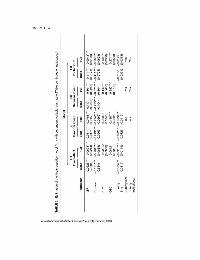
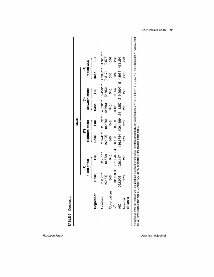
The results of the estimates are shown in Table 2 on the next page.The estimated models (base and full) show coefficients that are all statistically

significant and with signs consistent with our theoretical hypotheses (H0)–(H3), aftercontrolling for the institutional and size dummies, whose coefficients are not reported

18 The between effects (BE) estimator exploits exclusively the “between” dimension of the dateby regressing the individual averages of the dependent variable on the individual averages of thecovariates; the fixed effects (FE) estimate exploits solely the “within” dimension of the data by aregression in deviations from individual averages; the standard least squares estimator is appliedto the pooled data, which can be shown to be an (inefficient) average of the between and withinestimators; the random effects (RE) estimator, which is an efficient average of the between and withinestimators, while the weighting is based on the ratio of the variances of the individual specific effectand the stochastic disturbance.19 A time dummy variable may be useful to take into account the effect of the business cycleinfluences or technological changes even in a biannual model.

Research Paper www.risk.net/journal

90 G. Ardizzi

TAB

LE

2E

stim

atio

nof

the

linea

req

uatio

nm

odel

(4.1

)w

ithde

pend

entv

aria

ble:

cash

ratio

.[Ta

ble

cont

inue

son

next

page

.]

Mo

del

‚…„

ƒ(1

)(2

)(3

)(4

)F

ixed

effe

ctR

and

om

effe

ctB

etw

een

effe

ctP

oo

led

OL

S‚

…„ƒ

‚…„

ƒ‚

…„ƒ

‚…„

ƒR

egre

sso

rB

ase

Fu

llB

ase

Fu

llB

ase

Fu

llB

ase

Fu

ll

MIF

0.06

25���

0.06

24���

0.08

14���

0.07

88���

0.11

70.

101���

0.11

1���

0.09

43���

(0.0

204)

(0.0

214)

(0.0

171)

(0.0

159)

(0.0

245)

(0.0

245)

(0.0

171)

(0.0

170)

Turn

over

�0.

181����

0.18

1����

0.24

9����

0.27

4����

0.45

3����

0.57

1����

0.41

1����

0.50

8���

(0.6

84)

(0.0

688)

(0.0

569)

(0.0

569)

(0.1

04)

(0.1

04)

(0.0

704)

(0.0

698)

ATM

�0.

0091

20.

0608�

0.14

6���

0.13

4���

(0.0

650)

(0.0

346)

(0.0

430)

(0.0

308)

OT

C�

0.06

12�

0.19

6���

�0.

287���

�0.

274���

(0.1

03)

(0.0

594)

(0.0

790)

(0.0

563)

Dum

my

�0.

0259���

0.02

67���

0.02

26��

0.02

34��

�0.

0168

�0.

0175

time

(0.0

117)

(0.0

119)

(0.0

126)

(0.0

119)

(0.0

331)

(0.0

313)

Dum

my

size

Yes

Yes

Yes

Dum

my

Yes

Yes

Yes

inst

itutio

nal

Journal of Financial Market Infrastructures 1(4), Summer 2013

Card versus cash 91

TAB

LE

2C

ontin

ued.

Mo

del

‚…„

ƒ(1

)(2

)(3

)(4

)F

ixed

effe

ctR

and

om

effe

ctB

etw

een

effe

ctP

oo

led

OL

S‚

…„ƒ

‚…„

ƒ‚

…„ƒ

‚…„

ƒR

egre

sso

rB

ase

Fu

llB

ase

Fu

llB

ase

Fu

llB

ase

Fu

ll

Con

stan

t2.

283��

2.25

1��

2.87

4���

2.87

9���

4.52

8���

5.45

6���

4.20

0���

4.92

6���

(0.4

81)

(0.5

32)

(0.4

08)

(0.4

30)

(0.7

66)

(0.8

53)

(0.5

17)

(0.5

76)

Obs

erva

tions

546

546

546

546

546

546

546

546

R2

0.10

1/0.

894

0.10

3/0.

894

0.12

30.

223

0.13

10.

254

0.12

40.

235

AIC

�10

22.9

06�

1026

.117

116.

6754

109.

1199

241.

1257

219.

2909

514.

8956

461.

291

Num

ber

273

273

273

273

273

273

273

273

ofba

nks

All

varia

bles

ente

rth

ere

gres

sion

sin

loga

rithm

s.S

tand

ard

erro

rsro

bust

tohe

tero

sced

astic

ityar

ein

pare

nthe

ses.���p<

0.01

;��p<

0.05

;�p<

0.1.

Con

side

rR

2w

ithin

/ove

rall

adj-R

2fo

rth

efix

edef

fect

mod

el.C

onsi

der

AIC

the

ML

estim

ator

for

the

rand

omef

fect

mod

el.

Research Paper www.risk.net/journal

92 G. Ardizzi

for the sake of brevity.20 The negative sign of the time dummy variable seems to beconsistent with a linear trend of growth of card payments in Italy.

As expected, the coefficient of the interchange fee variable is consistently positive.The magnitude of the effect, moreover, is quite significant: a decrease of 10% in theMIF rate is associated with a reduction in the cash ratio of approximately 1%. Such anoutcome also represents an indirect test that the “interchange fee plus” mechanism ispresent and that interchange fees are not neutral.21 Such results seem to be consistentwith those obtained by Chakravorti et al (2009).

The value of turnover per card (“Turnover”) shows a significant negative impactupon the cash–card rate, as well as the higher relative diffusion of physical branches(OTC and ATM). The relevance of the ATM/card network dimension turns out to besignificant and positive, given that such a variable may be a proxy of the probabilitythat the intermediary intercepts the cards used at its own ATMs by providing freecash withdrawals.22 In the “fixed effect” model the ATM and OTC coefficients losesignificance. This can be partly explained by the fact that such (infrastructural) vari-ables do not vary significantly in the biennium, and the inclusion of the firm-specificdummy variables capture unobserved bank heterogeneity that is constant over time.

5.3 Robustness checks

We conducted several robustness checks of the outcomes illustrated in the previoussubsection, using alternative estimation methods that control for the presence of

(1) contemporary heteroscedasticity and autocorrelation of the residual terms,

(2) nonnormal distribution of the variables,

(3) endogeneity problems due to simultaneous causality or omitted variables.

Each of the above points highlights a violation of the assumptions underlying thelinear regression models and can make the results inconsistent.

20 The full model performs quite well also in term of fit: the F -statistics is significant at 1%;the overall adj-R2 tends to 0:89 in the fixed effect specification (least squares dummy variableregression); we will deal again with this issue in the robustness checks. Moreover, main results arerobust aggregating the information of the intermediaries that belong to the same banking group, inorder to control for possible “group” specific effects. For the sake of brevity, we do not present theresults of these tests, but they are available on request from the author.21 Based on empirical assessment of the Reserve Bank of Australia payment system reform, Hayes(2007) finds no significant impact of interchange fee level on the card usage. Nevertheless, thispartly contradicts Chang et al (2005) and Chakravorti et al (2009).22 This result is confirmed if we include ATM (expected sign: positive) and POS (expected sign:negative) separately in the model (see Table 5 on page 97).

Journal of Financial Market Infrastructures 1(4), Summer 2013

Card versus cash 93

The method used to control the first distortion factor, indeed, relies on properstatistical tests,23 we cannot reject the hypothesis of contemporary heteroscedasticityand cross-sectional and autocorrelation that can lead to biased statistical inference inthe panel (Cameron and Trivedi 2005). Therefore, in order to adjust the standard errorappropriately, we decide to apply the linear estimator with a panel-corrected standarderrors (PCSE) estimator suggested by Beck and Katz (1995). In particular, we specifythat, within groups, there is first-order autocorrelation and that the coefficient of theAR(1) process is specific to each group.24 In addition, we consider a standard OLSregression robust to bank-specific clustered standard errors.25

Regarding the second distortion,26 we consider a “quantile” regression estimator(“Quantile” estimator), where the relationship between y and x is not expressed bythe variation of the conditional mean of y given x (classical linear model), but by thevariation of one of its quantiles (eg, median). This approach is useful in the presenceof nonnormal distributions of the dependent variable, or of high statistical dispersion,which may make the mean value less significant. Furthermore, it may be interestingto calculate the impact of the MIF rate at different levels of the cash–card ratio (ie,25th or 75th percentile).27 For this method we have also resorted to the nonparametricbootstrap to calculate the standard errors and test the significance of the estimated

23 Specifically, we used the Wooldridge (2002) test for autocorrelation in panel data, the Greene(2000) test for groupwise heteroscedasticity and the Pesaran (2004) test for cross-sectional depend-ence in panel data.24 In particular, we consider the Prais–Winsten generalized least squares (GLS) estimator, derivedfor the AR(1) model for the error term, which represents a further innovation of the original OLSPCSE method proposed by Beck and Katz (Stata Technical Bulletin 1995).25 The usual OLS assumption is that standard errors are independently and identically distributed,but this assumption is clearly violated in many cases.A natural generalization is to assume “clusterederrors”, ie, that observations within groups (i banks) are correlated in some unknown way, inducingcorrelation in eit within i , but that groups i and j do not have correlated errors. In the GLS-PCSEmodel we also remove the latter assumption.26 A standard Shapiro–Wilk test for normality rejects such an assumption (Racine 2008). The methodmost appreciated when addressing the problem arising from nonnormal distribution of the variablesis nonparametric statistical techniques, which are robust to functional misspecification and do notrequire a researcher to specify functional forms for the objects being estimated. However, we leavethis extension to future research.27 The estimation for quantiles is conducted on the “pooled” panel, in order to gain degrees of free-dom. The quantile regression applied to panel models in fact requires a large sample size in order tounbundle the unobservable individual specific effects and produce consistent estimates (see Koenker2004). Also, differencing (or de-meaning) the data, as we would do under an OLS framework, isnot appropriate for quantile regressions: the quantiles of the sum of two random variables are notequal to the sum of the quantiles of each random variable. Moreover the interpretation given toindividual fixed effects is less appealing in quantile regression models, as the quantile regressionalready accounts for unobserved heterogeneity and heterogeneous effects.

Research Paper www.risk.net/journal

94 G. Ardizzi

TAB

LE

3R

obus

tnes

sch

ecks

agai

nstv

iola

tions

ofth

elin

ear

regr

essi

onas

sum

ptio

n.[T

able

cont

inue

son

next

page

.]

Mo

del

‚…„

ƒ(1

)(2

)(3

)(4

)(5

)(6

)(7

)(8

)(9

)

Lea

stS

qQ

uan

tile

‚…„

ƒ‚

…„ƒ

Reg

ress

or

FE

clu

ster

PC

SE

IVı

IVF

Eı

q5

q25

q50

q75

q95

MIF

0.06

43���

0.07

58���

0.11

12���

0.26

73���

0.07

310.

0735��

0.06

44���

0.08

49���

0.09

92���

(0.0

207)

(0.0

132)

(0.0

278)

(0.0

695)

(0.0

460)

(0.0

320)

(0.0

160)

(0.0

158)

(0.0

246)

Turn

over

�0.

154

�0.

357����

0.46

0����

0.02

2�

0.02

85�

0.44

6����

0.70

0�

0.88

9����

0.91

0���

(0.1

28)

(0.0

487)

(0.1

48)

(0.7

63)

(0.0

883)

(0.1

69)

(0.0

723)

(0.1

51)

(0.1

66)

ATM

�0.

0220

0.11

50.

1378���

0.08

260.

147��

0.13

9���

0.11

5���

0.08

140.

0467

(0.0

991)

(0.0

279)

(0.0

420)

(0.0

579)

(0.0

641)

(0.0

480)

(0.0

316)

(0.0

542)

(0.0

625)

OT

C�

0.04

06�

0.19

6����

0.28

9����

0.08

99�

0.15

6��

0.24

7����

0.28

5����

0.37

7����

0.36

7���

(0.1

07)

(0.0

240)

(0.0

864)

(0.1

199)

(0.0

879)

(0.0

539)

(0.0

426)

(0.0

928)

(0.1

23)

“Ira

te”

�0.

134����

0.10

7���

�0.

0741

�0.

106�

�0.

123���

0.26

7����

0.43

0���

(0.0

422)

(0.0

275)

(0.0

554)

(0.0

566)

(0.0

620)

(0.0

494)

(0.1

06)

Dum

my

time

�0.

0826����

0.06

37���

�0.

0055

�0.

113���

0.08

72����

0.06

30��

0.08

98����

0.09

38�

(0.0

198)

(0.0

121)

(0.1

600)

(0.0

521)

(0.0

330)

(0.0

332)

(0.0

246)

(0.0

556)

Dum

my

size

Yes

Yes

Yes

Yes

Yes

Yes

Yes

Dum

my

Yes

Yes

Yes

Yes

Yes

Yes

Yes

inst

itutio

nal

Journal of Financial Market Infrastructures 1(4), Summer 2013

Card versus cash 95

TAB

LE

3C

ontin

ued.

Mo

del

‚…„

ƒ(1

)(2

)(3

)(4

)(5

)(6

)(7

)(8

)(9

)L

east

Sq

Qu

anti

le‚

…„ƒ

‚…„

ƒR

egre

sso

rF

Ecl

ust

erP

CS

EIVı

IVF

Eı

q5

q25

q50

q75

q95

Con

stan

t1.

448

3.47

5���

4.40

6���

2.71

8���

0.68

73.

716���

5.47

4���

6.36

5���

6.40

8���

(1.0

49)

(0.5

12)

(1.1

712)

(0.8

125)

(0.8

05)

(1.2

36)

(0.5

69)

(1.2

95)

(1.6

36)

DW

H�

21.

4503

12.4

46�

——

——

—en

doge

neity

Firs

tsta

ge-F

201.

599���

8.98

7�—

——

——

rele

vanc

e

Sar

gan�

21.

668

0.18

3—

——

——

over

iden

tifyi

ngre

stric

tions

Obs

erva

tions

546

546

273

546

546

546

273

273

274

R2

0.14

/0.8

90.

840.

240.

08/0

.93

0.13

0.14

0.15

0.22

0.28

Ban

ks27

327

327

327

327

327

327

327

327

3

All

varia

bles

ente

rthe

regr

essi

ons

inlo

garit

hms.

Rob

usts

tand

ard

erro

rsar

ein

pare

nthe

ses.

For

quan

tile

regr

essi

ons,

stan

dard

erro

rsar

eba

sed

onbo

otst

rap

with

399

repl

icat

ions

.���p<

0.01

,��p<

0.05

,�p<

0.1.ıN

otes

:ins

trum

enta

lvar

iabl

esar

eth

efo

llow

ing.

2SLS

regr

essi

on(S

ourc

e:B

ank

ofIta

ly,b

anki

ngst

atis

tics)

;IV

–ra

ndom

effe

ct;i

nstr

umen

ted:

MIF

;ins

trum

ents

:MIFt�

1;T

urno

ver t�

1;N

etw

ork t�

1;a

sa

furt

her

robu

stne

ssch

eck,

sim

ilar

resu

ltsar

eob

tain

edif

we

cons

ider

the

follo

win

gal

tern

ativ

ein

stru

men

ts:M

IFt�

1,d

IMP

PO

S,d

IMPA

TM

;for

the

sake

ofbr

evity

,we

dono

tpre

sent

such

resu

ltsin

the

tabl

e.IV

FE

–fix

edef

fect

.Ins

trum

ente

d:M

IF,i

nstr

umen

ts:A

VG

_PO

S,N

etw

ork.

Lege

ndin

stru

men

tal

varia

bles

are

the

follo

win

g.N

etw

orkD

num

ber

ofAT

Ms

owne

d�

num

ber

ofca

rds

issu

ed.A

VG

_PO

SD

mea

nva

lue

ofth

eca

rdtr

ansa

ctio

nat

the

PO

Ss.

Research Paper www.risk.net/journal

96 G. Ardizzi

TABLE 4 Further robustness check against the assumption of exogeneity of the MIF:GMM estimator.

A B

Variableı GMM RE GMM FE

MIF 0.1545��� 0.3280��

N 273 546

�p < 0.1; ��p < 0.05; ���p < 0.01. ıFull model; all other explanatory (Zi ) variables are omitted. All variablesenter the regressions in logarithms. Robust standard errors are omitted. Generalized method of moments (GMM):A, size and institutional specific dummies included; B, individual fixed effect included.

coefficients without necessarily making assumptions about the probabilistic modeland the reference distribution of the sample.28

The third factor of distortion (simultaneous causality) is the possibility that therelationship between the cash–card rate and the interchange fee (or other covariates)is bidirectional or that there is nonzero contemporaneous correlation between theregressor(s) and the error term. For instance, if another unobserved variable jointlydetermines both a high cash–card ratio and high levels of interchange fees, the econo-metric models will not give consistent estimates. As noted above, the interchangefee variables are set by the self-regulatory body. Nevertheless, if some immeasurableaspects of the environment in which banks operate are associated with the acceptance,issuance or usage of cards, the risk of endogeneity bias in payment instruments analy-sis may increase (Chakravorti et al 2009). Thus, the standard Durbin–Wu–Hausman(DWH) test does not allow us to confirm the strict exogeneity of the MIF variable ifthe “fixed effect” estimator is applied, but only in the absence of firm-specific inter-cepts this assumption is not refuted.29 Accordingly, we also consider a two-stage leastsquares estimator (2SLS), using lagged values of the MIF and other selected variablesas instruments (see Chakravorti et al 2009).30

28 The results reported consider the regression on the 5th, 25th, 50th, 75th and 95th percentiles ofthe dependent variable.29 If the “firm-specific” intercepts are not included, the assumption of exogeneity is not refuted.However, we consider also the instrumental variable regression without individual “fixed effect”(see Table 3 on page 94).30 Other instrumental variables are the current value of the average transaction at POSs (see Table 3on page 94), which may affect the average interchange fee levels (relevance condition) and shouldnot necessarily be correlated with the error term in (4.1) (validity condition), as confirmed by“first stage” 2SLS test (Hausman) and the Sargan–Hansen of overidentifying restriction test (seeWooldridge 2002). Moreover, we also consider the (lagged) instrumental variable “network” (equalto the product of the number of ATMs and the number of cards managed by the issuing bank) andthe lagged value of the “Turnover”.

Journal of Financial Market Infrastructures 1(4), Summer 2013

Card versus cash 97

TABLE 5 Further robustness check of stability to perturbations in the parameters (alter-native specification of the model and GMM estimator).

Model‚ …„ ƒ(1) (2) (3) (4)

Variable RE FE GMM IVRE GMM IVFE

MIF 0.0811��� 0.0719��� 0.1248��� 0.1683�

Turnover �0.2900��� �0.1724 �0.5998��� �0.1196ATM 0.1162��� �0.0923 0.2044��� �0.0935Pos �0.0935��� �0.1522��� �0.0449N 546 546 273 546

�p < 0.1; ��p < 0.05; ���p < 0.01. All variables enter the regressions in logarithms. Robust standard errors areomitted.Additional variables:ATMD (log) number of ATMs;PosD (log) number of POSs.Models (1) and (3) have sizeand institutional specific dummies included. Models (2) and (4) have individual fixed effects included. Instrumentalvariables for GMM models: A, (3), random effect. Instrumented: MIF. Instruments: MIFt�1, Turnovert�1, Networkt�1.As a further robustness check, similar results are obtained if we consider the following alternative instruments:MIFt�1, dIM PPOS, dIMP ATM; for the sake of brevity, we do not present such results in the table. B, (4), fixed effect.Instrumented: MIF. Instruments: AVG_POS, Network. Legend instrumental variables: network D number of ATMsowned � number of cards issued. AVG_POS D mean value of the card transaction at the POSs.

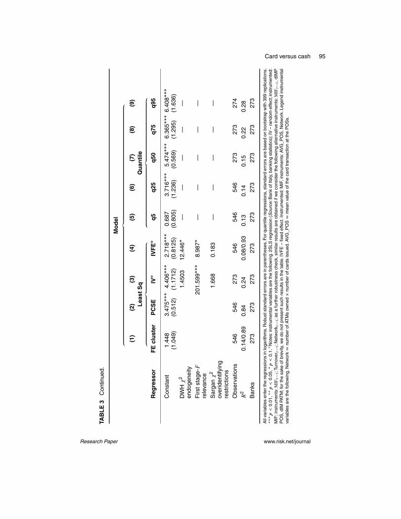
The outcomes relative to the different robust estimators31 are reported in Table 3on page 94.

As a result, the robustness checks seem to be more than satisfactory. Across all ofthe methods adopted, the significance and the intensity (positive) of the MIF effect onthe cash–card rate (cash ratio) are confirmed.32 Moreover, the inclusion of the (proxy)of the interest rate does not affect the main results.33

31 Least absolute deviation methods (quantile regression) may be affected by endogeneity problemas well. However, this issue is not well developed in literature yet and beyond the scope of this firstempirical investigation.As a further test of robustness, we limit to apply the (two-stage) instrumentalvariable quantile regression model proposed by Chernozhukov and Hansen (2008), who recentlyintroduced an ad hoc command in the Stata Software, considering the same instrumental variablesincluded in the instrumental variable least squares regression. Such an extension confirms the mainconclusions of this paper and results are available upon request.32 The selection of the “full” model as the best one is supported by the Akaike information criterion(AIC). However, the AIC measure gives less support to the model including interest rates togetherwith the time dummy. The time dummy intercept is indeed significantly correlated (Pearson’scorrelation coefficient:C0:46) with the interest rate variation across the two years.33 Recall that a proxy of the interest rate has been included just as a test of stability of the estimatesshown in Section 5.2. However, all the estimates shown in Table 3 on page 94 have been replicatedwithout the “interest rate” variable and no significant changes in the relevant coefficients have beenfound. For the sake of brevity, we do not present such results.

Research Paper www.risk.net/journal

98 G. Ardizzi

The magnitude of the marginal effect of the interchange fee rate is stronger andmore significant for banks in the upper tail of the distribution (quantile regression)34

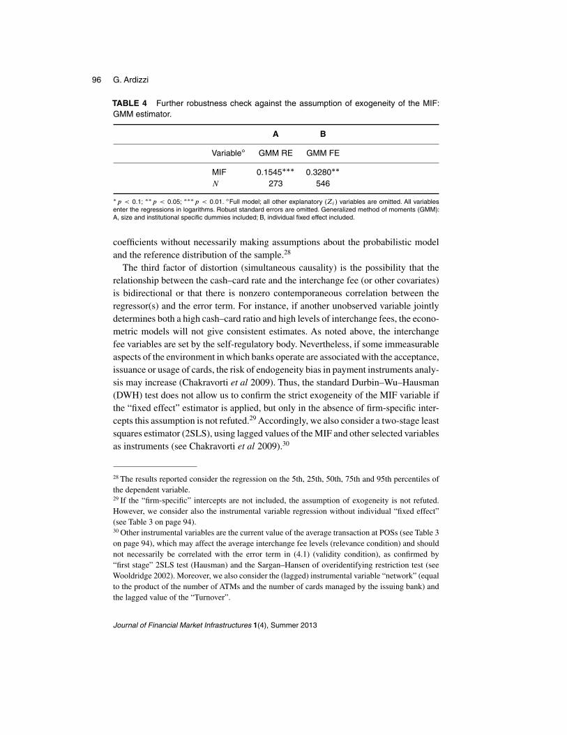
and after controlling for endogeneity in the instrumental variable (IV) least squaresestimation35 (Table 3 on page 94). Finally, we replicated the regressions through thegeneralized method of moments (GMM) method developed by Hansen, which is lessaffected by the distributional assumptions (such as normality) than the 2SLS andmay be more efficient in the presence of heteroscedasticity of unknown form andweak instruments (Wooldridge 2002). In addition, we further tested the sensitivityof the model to perturbations of the parameters by removing hypothesis (H3) andadopting an alternative specification to control for the network effects: we added thenumber of POSs together with the number of ATMs (without normalization) amongthe covariates. The main results are confirmed and summarized in Table 4 on page 96and Table 5 on the preceding page36

6 WHAT ABOUT THE OPTIMAL MULTILATERAL INTERCHANGEFEE? FIRST EVIDENCE FROM A NONLINEAR APPROACH

As discussed in our review of the literature, one relevant policy issue is concerned withthe determination (or regulation) of the optimal level of interchange fee. For instance,according to Rochet and Tirole (2008), an MIF reduction may be translated as anincrease in the cardholder fees with a negative net impact on the “social welfare func-tion”, which is a single-peaked function including different components (consumersurplus, retailers’ profit and banks’ profit). This means (Rochet and Tirole 2008) thatthe optimal interchange fee (MIF�) that maximizes the social welfare function maybe nonzero (Figure 6 on the facing page).

Since there was a risk that card payment schemes set excessively high interchangefees to increase banks’ profits, the competition authorities started to limit exces-

34 It is interesting also to note that the (negative) estimated coefficient for “Turnover” increasesmonotonically and considerably for the upper quantiles’ regressions, suggesting that the incomeeffect on the demand for cash is stronger for banks in the upper tail of the distribution.35 As in the standard FE estimations, the estimated coefficients of the control variables lose con-sistency in the IVFE specification, but we cannot exclude that this is due to their collinearity withthe individual specific intercepts and the limited “within variability” in the biannual panel. We alsoexcluded the interest rate in the IV regression models, to reduce endogeneity problems.36 The diagnostic tests for endogeneity and overidentifying restrictions in the GMM estimates(Table 4 and Table 5) are consistent with the ones obtain in the 2SLS estimates (Table 3). Wealso remove the “I rate” variable, which is not robust to the test for the orthogonality/exogeneitycondition in the GMM model (Sargan). All these results are available upon request from the author.

Journal of Financial Market Infrastructures 1(4), Summer 2013

Card versus cash 99

FIGURE 6 Interchange fee and social welfare.

Interchange feeMIF* > 00

W (

soci

al w

elfa

re)

Source: Rochet and Tirole (2011).

sive interchange fees through the cost-based regulation or the implementation of the“tourist test”, but always admitting positive levels of interchange fee in the system.37

Nevertheless, in recent years the debate has focused on the issue of whether the MIFon the modern card networks should be dismissed or maintained. Some economistsclaim that the interchange fee should be reduced to zero so as to remove direct andindirect regulatory costs to the market participants (Gans 2007) and to promote bothcompetition and efficiency in retail payments, as compared to a situation with positiveinterchange fee (Leinonen 2009).

The theoretical problem of the optimal interchange fee determination is beyondthe scope of the present paper. We can just find some clues through a more in-depthinvestigation of the relationship between the cash demand and the MIF according toour model analysis. Indeed, the cash–card ratio may be taken as a practical indicatorfor a social planner who is interested in shifting from cash to electronic payments.

In order to delve deeper into the effective impact of the interchange fee on thechoice of payment instruments, as a first descriptive investigation we consider themultivariable scatter plot smoother (nonparametric approach),38 which is a valuable

37 Rochet (2007) states that “competition authorities often care only about user surplus and not aboutsocial welfare. This is justified if the profit of firms (banks) is completely dissipated. This is notjustified if profit is reinvested to provide quality of service or attracts entry (lower prices, increasedproduct variety)”.38 The methods most appreciated when addressing the problem arising from nonlinear relationshipsare the nonparametric statistical techniques, which are robust to functional misspecification (ie,linear or polynomial). However, we leave this extension to a future research. In this case we adopteda nonparametric method called “k-nearest neighbours” or “k-nn”, which is available through thesoftware Stata 10 (Royston and Cox 2005). In this case, a simple estimator (corresponding to auniform kernel) is to take the k observations nearest to x, and fit a linear regression of yi on Xi

Research Paper www.risk.net/journal

100 G. Ardizzi

FIGURE 7 Multivariable scatter plot smoother.

–1

0

1

2

3ln

cas

h ra

tio

–9 –8 –7 –6 –5 –4

ln MIF

Multivariate nearest-neighbour smoother; other explanatory variables contained in (4.1), including bank-specific andtime dummy variables, are omitted in the figure.The upper and lower lines represent a pointwise confidence interval(95ı) for the smoothed values of “cash ratio”.

tool in exploratory data analysis (when the aim is to arrive at a parametric final model)and does not require us to specify functional forms for objects being estimated andstrongly increases the goodness of the fit (Royston and Cox 2005). This graphicaltool allows us to obtain a picture of the relationship between the “cash ratio” and MIFof (4.1) and each of the other explanatory variables simultaneously. The fitted (log)values of the cash–card ratio conditioned to the (log) average transaction-weightedMIF rate are shown in Figure 7.

Consistent with the findings reported in the previous sections, the MIF and thepreference for cash withdrawal tend to be positively correlated. Nevertheless, thisrelationship is neither linear nor strictly monotonic: it is only beyond a certain levelthat the MIF impact is binding and the relationship with the cash–card ratio becomesstrictly positive.

That being said, starting from Figure 7 we can try to estimate parametrically thenonlinear (second-order) effect of the MIF by adding a quadratic term in the original

using these observations. A smooth local linear k-nn estimator fits a weighted linear regression (seeHansen 2012).

Journal of Financial Market Infrastructures 1(4), Summer 2013

Card versus cash 101

TABLE 6 Estimation of the quadratic equation model (6.1).

Modelı‚ …„ ƒA B C D E F

Regressor1 PCSE2 FE3 RE4 IVRE5 OLS6 q507

MIF 0.1564��� 0.0727��� 0.1057��� 0.4579��� 0.1961��� 0.1641���

(0.0421) (0.0253) (0.0228) (0.1304) (0.0264) (0.0248)MIF2 0.0639��� 0.0229� 0.0375��� 0.1716��� 0.0750��� 0.0565���

(0.0208) (0.0121) (0.011) (0.0511) (0.0126) (0.0124)Adj-R2 0.8526 0.8953 0.2761 0.1708

Estimated turning points(ln) MIF� �6.55 �6.91 �6.73 �6.66 �6.63 �6.78MIF� 0.0014 0.0010 0.0012 0.0013 0.0013 0.0011

ı“Full” model, MIF variable is log transformed and normalized on the sample mean; all other explanatory (Zi )variables are omitted. All variables enter the regressions in logarithms. Significance: ���p < 0.01, ��p < 0.05,�p < 0.1.Robust standard errors are in parentheses. 1MIF variable is log transformed and normalized on the samplemean. Other explanatory variables (Zi ) contained in (6.1), including bank-specific and time dummy variables, areomitted in the table. 2Panel corrected standard error estimator. 3Fixed effect estimator. 4Random effect estimator5Instrumented random effect estimator. Instrumented: MIF. Instruments: MIFt�1, turnovert�1, networkt�1. 6OLSestimator. 7Quantile regression (50ı percentile).

equation model of (4.1), as follows:39

cash ratioit D ˛0 C a1MIFit C a2MIF2 CX

h

˛hZit C uit : (6.1)

Whereas MIF and its squared term are strongly correlated (r D j0:94j), we havenormalized the variable on its sample mean before taking its logarithm in order toreduce collinearity problems. Hence, we estimate (6.1) through the methods proposedin the previous sections.40 For brevity, we just report estimated coefficients for thelinear and quadratic MIF term (see (6.1)).

The outcomes in Table 6 show that the estimated regression coefficients for thefirst-order and second-order effects of the MIF are both positive and significant. Thismeans that the cash ratio–MIF linear slope gets more positive as the MIF increases,the quadratic in MIF has a hump shape and the turning point (Wooldridge 2002) in

39 We are indebted to an anonymous referee for this suggestion.40 We selected the following methods: ordinary least squares (OLS), quantile regression (q50),panel data random effect (RE) and fixed effect (FE), also controlling for autocorrelation and cross-sectional dependence (PCSE) and instrumental variable GMM random effect estimator to take intoconsideration endogeneity problems. As we show in Section 5.3 (see footnote 35 on page 98), alsoin this case we exclude the IVFE specification, because of a collinearity problem with the quadraticterm and the individual specific intercepts and the limited “within variability” in the biannual panel.

Research Paper www.risk.net/journal

102 G. Ardizzi

the single peak response probability is equal to Œa1�=.2a2/ > 0.41 Accordingly, theturning point, at which we have the minimum (fitted) value of cash ratio, is positiveand different from zero MIF. This outcome seems to be consistent with the theoreticalframework provided by Rochet and Tirole (2002, 2003).Although they do not considerthe “cash–card ratio” explicitly in their model, our cash–card ratio may decrease untilreaching the turning point. However, further empirical investigations are needed onthis issue, such as in the case of the longer confidence interval for the smoothed valuesof “cash ratio” in Figure 7 on page 100, due to higher dispersion of the data at thelower tail of the MIF levels.42

Finally, the estimated turning point in the quadratic function (or “threshold level”)is always much lower than the actual mean level of the MIF as reported in Table 6on the preceding page and Table 1 on page 86, respectively. This means that thequadratic in MIF is positively skewed for a long stretch and that the positive lineartrend, discussed in the previous section, is predominant.

7 CONCLUSION

The multilateral setting of interchange fees is usually justified because it reducesnetwork transaction costs and increases payment card usage. Some economists andantitrust decisions also show how the interchange fee is an intermediary cost used asa reference price for the final fee charged to merchants (the so-called interchange feeplus mechanism). Nevertheless, few empirical works have measured the net impactof the interchange fee on the end user’s decision to pay by card or withdraw cash.

Starting from our model of analysis, we consider the “cash–card ratio” as a prac-tical reference indicator for a social planner who is interested in shifting from cashto electronic transactions. This would be consistent with the position expressed byseveral central banks, affirming that a strong shift to payment card transactions inlieu of cash would reduce the overall social cost of the payment industry and increasesavings for payment service providers, firms and consumers. In Italy the cash–cardratio is higher than the average level in Europe. Thus, the main objective of this paperis to conduct a first empirical investigation on the impact of the interchange fee onthe choice of cash withdrawals over card purchases for POS payments. This allowsus to confirm that a regulation of the MIF level may be an effective tool in reducingthe cash payments at the POSs.

Our results and robustness checks show that there is a positive relationship betweencash usage and interchange fee mechanism, and that current mean MIF levels are still

41 As the MIF variable is logarithmically transformed and normalized on the sample mean, theturning point is calculated as follows: expŒ.a1=2a1/Cmean.MIF/�.42 This can be also confirmed by the parametric regressions.

Journal of Financial Market Infrastructures 1(4), Summer 2013

Card versus cash 103

too high to foster card acceptance in lieu of cash. Such a result is consistent with thoseobtained by Chakravorti et al (2009). Furthermore, from a first empirical investigation,such a relationship is not strictly monotonic, especially at the lower tails of the MIFlevel distribution.

Hence, we cannot also affirm that a zero MIF level would be optimal to increaseelectronic transactions, and we leave this topic for future research. We note thata relevant part of the economic literature perceives that a zero MIF rate may becounterproductive for the payment card diffusion and this may compromise the marketincentive for innovation (Rochet 2007).

Finally, although the problem of the optimal interchange fee determination isbeyond the scope of the present paper, our empirical model may inspire furtherresearch on the issue of interchange fee regulation. Indeed, our approach encour-ages investigation of the impact of different MIF rates on the substitutability betweendifferent means of payments, through relevant information collected on the issuingside. This payment data is usually more reliable and easy to obtain from the regulationauthorities and our simple method of analysis may give some clues for how to enhancethe efficiency of the payment system. For instance, policymakers may define somescenario analysis with the results of changes in the cash ratio as a result of changesin the average MIF.

REFERENCES

Alvarez, F., and Lippi. F. (2009). Financial innovation and transactions demand for cash.Econometrica, 77(2), 363–402.

Ardizzi, G., and Coppola, G. (2002). The Italian case study: interchange fee, market struc-ture and cost efficiency in the retail payment system. Conference on “The Economics ofPayment Networks”. Working Paper, IDEI Université de Toulouse I.

Banca d’Italia (1998). Provision number 23 of 8 October 1998 – PAGOBANCOMAT.Banca d’Italia (2012a). The social cost of payment instruments in Italy. Institutional Issues

(November).Banca d’Italia (2012b). Annual Report 2011.Baxter, W. F. (1983). Bank interchange of transactional paper: legal and economic perspec-

tives. Journal of Law and Economics 26(3), 541–588.Beck, N., and Katz, J. (2004). Time-series–cross-section issues. Working Paper.Bolt, W., and Schmiedel, H. (2013). Pricing of payment cards, competition, and efficiency:

a possible guide for SEPA. Annals of Finance 9(1), 5–25.Bolt, W., Humphrey, D., and Uittenbogaard, R. (2008).Transaction pricing and the adoption

of electronic payments: a cross-country comparison. International Journal of CentralBanking 4(1), 89–123.

Bolt, W., Jonker, N., and van Renselaar, C. (2010). Incentives at the counter: an empiri-cal analysis of surcharging card payments and payment behaviour in the Netherlands.Journal of Banking and Finance 34(8), 1738–1744.

Research Paper www.risk.net/journal

104 G. Ardizzi

Börestam, A., and Schmiedel, H. (2011). Interchange fee in card payments. OccasionalPaper, European Central Bank.

Breusch, T. S., and Pagan A. R. (1980). The Lagrange multiplier test and its application tomodel specifications in econometrics. Review of Economic Studies 47(1), 239–253.

Cameron, C., and Trivedi, K. P. (2005). Microeconometrics: Methods and Applications.Cambridge University Press.

Chakravorti, S., Fernandez, F.R., andValverde, S.C. (2009).Regulating two-sided markets:an empirical investigation. Working Paper, Federal Reserve Bank of Chicago.

Chang, H., Evans, D., and Garcia-Swartz, D. (2005). The effect of regulatory interventionin two-sided markets: an assessment of interchange-fee capping in Australia. Review ofNetwork Economics 4(4).

Chernozhukov, V., and Hansen, C. (2008). Instrumental variable quantile regression: arobust inference approach. Journal of Econometrics 142(1), 379–398.

Coppola, G. (2011). Le surcharge sulle carte di pagamento. Studi e Note di Economia16(3), 323–340.

Doria, M. (2010). L’obiettivo di riduzione del contante: la facoltà di applicare “sconti” perl’acquisto di beni o servizi; il divieto di “surcharge”. In La Nuova Disciplina dei Servizi diPagamento. Giappichelli, Torino.

European Central Bank (2006). The Eurosystem’s view of a SEPA for cards. OccasionalPaper.

European Central Bank (2012). Payment statistics. Report incorporating 2011 data. ECB,September.

European Commission (2010). Decision relating to proceedings under Article 101 of theTreaty on the Functioning of the European Union and Article 53 of the EEA Agreement.Case COMP/39.398, Visan MIF.

European Commission (2012). Toward an integrated market for card, internet and mobilepayments. Green Paper, COM(2011) 941.

Evans, D. S., and Schmalensee, R. L. (1999). Paying with Plastic. MIT Press, Cambridge,MA.

Gans, J. S. (2007). Evaluating the impact of the payment system reforms. Submission tothe Reserve Bank of Australia’s Payment System Board’s 2007–08 Review of PaymentSystem Reforms.

Gans, J. S., and King, S. P. (2003). The neutrality of interchange fees in payment systems.Topics in Economic Analysis and Policy 3, Article 1.

Greene, W. (2000). Econometric Analysis. Prentice-Hall, Englewood Cliffs, NJ.Hansen, B. (2012). Econometrics. University of Wisconsin.Hayes, R. (2007). An econometric analysis of the impact of the RBAs credit card reforms.

Mimeo, Melbourne Business School.Hoechle, D. (2007). Robust standard errors for panel regressions with cross-sectional

dependence. Stata Journal 7(3), 281–312.Humphrey, D. B., Pulley, L. B., and Vesala, J. M. (1996). Cash, paper, and electronic pay-

ments: a cross-country analysis. Journal of Money, Credit and Banking 8(4, Part 2),914–939.

ITM (2000). Study regarding the effects of the abolition of the non-discrimination rule inSweden. European Commission Directorate General for Competition.

Journal of Financial Market Infrastructures 1(4), Summer 2013

Card versus cash 105

Jones, P., and Jones, C. (2006). Explaining differing European MCS levels. Papeles deEconomia Espanola.

Jonker, N. (2011). Card acceptance and surcharging: the role of costs and competition.Working Paper 300, De Nederlandsche Bank.

Koenker, R. (2004). Quantile regression for longitudinal data. Journal of Multivariate Analy-sis 91(1), 74–89.

Leinonen, H. (2007). On the efficiency of multilateral interchange fees (MIFs): how to pricecash and cards in order to promote payment efficiency. Bank of Finland Online, no. 4.Financial Markets and Statistics.

Leinonen, H. (2011). Debit card interchange fees generally lead to cash-promoting cross-subsidisation. Bank of Finland Online, no. 3. Financial Markets and Statistics.

Lippi, F., and Secchi, A. (2009). Technological change and the households’ demand forcurrency. Journal of Monetary Economics 56, 222–230.

Pesaran, M. H. (2004). General diagnostic tests for cross section dependence in panels.Working Paper, University of Cambridge.

Racine, J. S. (2008). Nonparametric econometrics: a primer. Foundations and Trends inEconometrics 3(1), 1–88.

Rochet, J.-C. (2007). Understanding interchange fees. Mimeo, Toulouse School of Eco-nomics and IDEI.

Rochet, J.-C., and Tirole, J. (2002). Cooperation among competitors: some economics ofpayment card associations. RAND Journal of Economics 33(4), 549–570.

Rochet, J.-C., and Tirole, J. (2003). Platform competition in two-sided markets. Journal ofthe European Economic Association 1(4), 990–1029.

Rochet, J.-C., andTirole, J. (2011).Must-take cards:merchant discounts and avoided costs.Journal of the European Economic Association 9(3), 462–495.

Royston, P., and Cox, N. J. (2005). A multivariable scatterplot smoother. Stata Journal 5(3),405–412.

Schmiedel, H., Kostova, G., and Ruttenburg, W. (2012).The social and private cost of retailpayments: a European perspective. Occasional Paper, European Central Bank.

Stata Technical Bulletin (1995). Stata Technical Bulletin, STB-25 (May).Stix, H. (2004). How do debit cards affect cash demand? Survey data evidence. Empirica

31(2–3), 93–115.Visa International (2001). Visa International Service Association. Mimeo.Wooldridge, J. M. (2002). Econometric Analysis of Cross Section and Panel Data. MIT

Press, Cambridge, MA.Zenger, H. (2011). Perfect surcharging and the tourist test interchange fee. Journal of

Banking and Finance 35(10), 2544–2546.

Research Paper www.risk.net/journal