multi-phase resilience assessment and adaptation of...
TRANSCRIPT

PONTIFICIA UNIVERSIDAD CATOLICA DE CHILE SCHOOL OF ENGINEERING
MULTI-PHASE RESILIENCE
ASSESSMENT AND ADAPTATION OF
ELECTRIC POWER SYSTEMS
THROUGHOUT THE IMPACT OF
NATURAL DISASTERS
SEBASTIAN ANDRES ESPINOZA
Thesis submitted to the Office of Research and Graduate Studies in
partial fulfilment of the requirements for the Degree of Master of
Science in Engineering
Advisor: HUGH RUDNICK VAN DE WYNGARD
Santiago de Chile, October 2015.
© MMXV, Sebastián Andrés Espinoza Lara

PONTIFICIA UNIVERSIDAD CATOLICA DE CHILE SCHOOL OF ENGINEERING
MULTI-PHASE RESILIENCE
ASSESSMENT AND ADAPTATION OF
ELECTRIC POWER SYSTEMS
THROUGHOUT THE IMPACT OF
NATURAL DISASTERS
SEBASTIAN ANDRES ESPINOZA
Members of the Committee:
HUGH RUDNICK VAN DE WYNGARD
DANIEL OLIVARES QUERO
RODRIGO MORENO VIEYRA
MIGUEL RIOS OJEDA
Thesis submitted to the Office of Research and Graduate Studies in
partial fulfilment of the requirements for the Degree of Master of
Science in Engineering
Santiago de Chile, October 2015.

ii
DEDICATION
To my loving sister, mother and grandmother.

iii
ACKNOWLEDGEMENTS
I would like to express my deepest gratitude to my advisor, Professor Hugh
Rudnick, not only for his constant support and guidance in the past years, but also because
through his example he has shown me different ways to serve those around me.
Special thanks to Mathaios Panteli and Professor Pierluigi Mancarella from The
University of Manchester, who have been working in the Electric Power Systems group
together with Tyndall Centre for Climate Change trying to tackle global problems. I am
much obliged for the co-work and for receiving me in Manchester for a semester.
Also thanks for the co-work to Felipe Rivera, Alan Poulos, Paula Aguirre, Jorge
Vásquez, Juan Gonzáles and the dean Juan Carlos de la Llera from CIGIDEN, who are
developing scientific knowledge that will enable Chile to be better prepared to confront
natural disasters. My gratitude to Rodrigo Moreno from University of Chile for his kind
academic and personal advises. Thanks to Óscar Alamos from the Ministry of Energy,
Helia Vargas from ONEMI, Mark Beswick from the MET UK Office, Jorge Araya from
GSI and Juan Carlos Araneda, Raúl Moreno and Marco Quezada from CDEC-SING.
Also my gratitude to Carlos Medel, Alejandro Navarro, Luis Gutierrez and Carlos
Cruzat for having the time to answer my questions and all the people in The University of
Manchester for making me feel at home. Thanks to the past and present friends of the
Office 302, where we had endless days discussing how to solve the energy problems of the
world. And of course, thanks for the constant support of my girlfriend Pía and my life-
friends. Thanks especially to my family for every little detail that have made me who I am.
Thanks to all for all those afternoons that you gave to this project without thinking
in what you would receive back.
I finally hope this research is a small contribution to the disaster management and
electric power systems fields. Chile and countries affected by major natural disasters need
to improve their actions at the preparedness, response, recovery and mitigation stages
while having a special care for those in need within the society, who are at the same time
the most affected.
”Pray as though everything depended on God. Work as though everything
depended on you”. - Saint Augustine

TABLE OF CONTENTS
Page
DEDICATION ............................................................................................................. ii!
ACKNOWLEDGEMENTS ........................................................................................ iii!
LIST OF FIGURES .................................................................................................... vii!
LIST OF TABLES ...................................................................................................... ix!
ABSTRACT ................................................................................................................. x!
RESUMEN .................................................................................................................. xi!
1.! INTRODUCTION ............................................................................................... 12!1.1! Motivation ................................................................................................ 12!1.2! Objectives ................................................................................................. 12!1.3! Research delimitations ............................................................................. 13!1.4! General methodology ............................................................................... 15!1.5! Thesis outline ........................................................................................... 16!
2.! BASIC CONCEPTS ............................................................................................ 17!2.1! Definitions ................................................................................................ 17!2.2! System’s performance curve throughout a disaster .................................. 18!2.3! Electric power system’s structure ............................................................ 19!2.4! Types of risk analyses .............................................................................. 20!
3.! STATE OF THE ART AND CONTRIBUTIONS OF THIS THESIS ............... 22!3.1! Different perspectives for the resilience concept ..................................... 22!3.2! Methodological advances of resilience assessment and
adaptation in electric power systems ........................................................ 23!3.3! Contributions of the present work ............................................................ 24!
4.! MULTI-PHASE RESILIENCE ASSESSMENT AND ADAPTATION FRAMEWORK ................................................................................................ 26!4.1! Multi-phase resilience assessment ........................................................... 26!
4.1.1! Phase one: threat characterization .................................................. 27!

4.1.2! Phase two: vulnerability of system’s components ......................... 29!4.1.3! Phase three: system’s reaction ....................................................... 31!4.1.4! Phase four: system’s restoration .................................................... 32!
4.2! Multi-phase adaptation strategies ............................................................. 32!4.3! Resilience metrics .................................................................................... 34!4.4! Resilience modelling ................................................................................ 34!
5.! APPLICATION TO WINDSTORMS AND FLOODS IN GREAT BRITAIN . 36!5.1! Influence of extreme weather and climate change in Great Britain’s
power system ............................................................................................ 36!5.1.1! Extreme weather events ................................................................. 36!5.1.2! Climate change and future hazard scenarios .................................. 37!
5.2! The Great Britain’s simplified electric power system .............................. 38!5.3! Resilience assessment .............................................................................. 39!
5.3.1! Phase one: windstorms and floods characterization ...................... 39!5.3.2! Phase two: vulnerability of electrical components ........................ 42!5.3.3! Phase three: power system’s reaction ............................................ 44!5.3.4! Phase four: power system’s restoration ......................................... 45!
5.4! Resilience adaptation ................................................................................ 46!5.5! Results and discussion .............................................................................. 47!
6.! APPLICATION TO EARTHQUAKES IN CHILE ............................................ 50!6.1! Influence of earthquakes and tsunamis in Chile ....................................... 50!
6.1.1! Influence of earthquakes in Chile’s power systems ....................... 51!6.1.2! Future hazard scenarios in northern Chile ..................................... 53!
6.2! The northern Chilean reduced electric power system .............................. 54!6.3! Resilience assessment .............................................................................. 57!
6.3.1! Phase one: earthquakes characterization ........................................ 57!6.3.2! Phase two: vulnerability of electrical components ........................ 58!6.3.3! Phase three: power system’s reaction ............................................ 61!6.3.4! Phase four: power system’s restoration ......................................... 63!
6.4! Resilience adaptation ................................................................................ 64!6.5! Results and discussion .............................................................................. 65!
7.! CONCLUSIONS ................................................................................................. 69!

8.! FUTURE WORK ................................................................................................ 71!
REFERENCES ........................................................................................................... 73!
A P P E N D I C E S ................................................................................................... 82!
APPENDIX A : CORRELATION BETWEEN ELECTRICITY CONSUMPTION AND ECONOMIC GROWTH ......................................................................... 83!
APPENDIX B : MULTI-PHASE RESILIENCE AND ADAPTATION FRAMEWORK ................................................................................................ 84!
APPENDIX C : EARTHQUAKE AND TSUNAMI 2015 ........................................ 85!
APPENDIX D : SOIL CLASSIFICATION OF NORTHERN CHILE ..................... 87!
APPENDIX E : NORTHERN CHILEAN HAZARD MAP ...................................... 88!
APPENDIX F : INTERNATIONAL LITERATURE OF SEISMIC FRAGILITY CURVES FOR ELECTRICAL COMPONENTS ............................................ 89!
APPENDIX G : SING’S RECUPERATION ZONES ............................................... 91!
APPENDIX H : LIST OF PUBLICATIONS AND PRESENTATIONS .................. 92!

vii
LIST OF FIGURES
Page
Figure 2.1. System’s performance curve throughout a disaster .......................................... 18!
Figure 2.2. Electric power system’s structure ..................................................................... 19!
Figure 2.3. Types of system risk analyses ........................................................................... 21!
Figure 4.1. The multi-phase resilience and adaptation framework ..................................... 26!
Figure 4.2. Generic fragility curve: probability of failure vs threat parameter ................... 30!
Figure 4.3 (a). Different fragility curves to assign damage states. (b). Different zones in the fragility curve to assign damage states ................................................................... 31!
Figure 4.4 (a). Normal case. (b). Robust case. (c). Redundant case. (d). Responsive case. 33!
Figure 4.5. Resilience modelling flow chart ....................................................................... 35!
Figure 5.1 (a). Great Britain’s simplified system. (b). Weather regionalization of the system. ......................................................................................................................... 38!
Figure 5.2. Winter peak demand week in Great Britain ...................................................... 39!
Figure 5.3. Projection diagram for Region 4 ....................................................................... 41!
Figure 5.4. (a) Lines and tower’s fragility curves. (b) Floods by intense or prolonged rainfall fragility curves ................................................................................................ 43!
Figure 5.5. Dotted lines show the critical transmission corridor for which the adaptation case studies are applied ............................................................................................... 46!
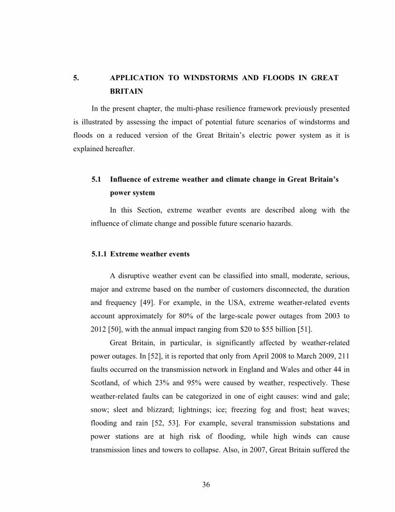
Figure 5.6. EENS of different hazards in potential future scenarios ................................... 47!
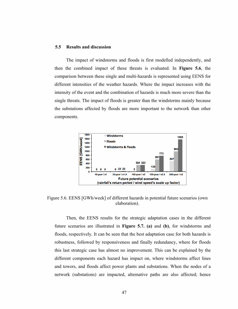
Figure 5.7. (a) Windstorms adaptation strategies results. (b) Floods adaptation strategies results. ......................................................................................................................... 48!

viii
Figure 5.8. (a) Windstorms adaptation results improvements for the three most hazardous events. (b) Floods adaptation results improvements for the three most hazardous events. ........................................................................................................ 48!
Figure 6.1. (a) Number of medium shallow earthquakes plotted against latitude. (b) Map of all earthquakes registered by USGS from 1973 to 2012 ......................................... 54!
Figure 6.2. (a) Northern Chile real system. (b) Northern Chile explicative diagram.. ....... 55!
Figure 6.3. Northern Chilean reduced electric power system ............................................. 56!
Figure 6.4. Transmission tower’s fragility curves. ............................................................. 60!
Figure 6.5. Anchored medium voltage substation’s fragility curves .................................. 60!
Figure 6.6. Anchored low voltage substation’s fragility curves ......................................... 60!
Figure 6.7. Anchored large power plant’s fragility curves ................................................. 61!
Figure 6.8. Anchored small power plant’s fragility curves ................................................. 61!
Figure 6.9. Annual peak demand week in the SING. .......................................................... 62!
Figure 6.10. Generation capacity and reserves normative. ................................................. 63!
Figure 6.11. Northern Chilean system with GIS information ............................................. 65!
Figure 6.12. Hourly expected power not supplied. ............................................................. 66!
Figure 6.13. Hourly power net capacity .............................................................................. 67!
Figure 6.14. EENS of the normal system under different scenarios. .................................. 68!
Figure 6.15. EIU of adaptation strategies under different scenarios. .................................. 68!

ix
LIST OF TABLES
Page
Table 5.1. Threats analysed with their correspondent key vulnerable components identified. .................................................................................................................... 42!
Table 5.2. Mean times to repair (hours) for different weather intensities ........................... 45!
Table 5.3. EIU results .......................................................................................................... 49!
Table 6.1. Hazard analysed with its correspondent key vulnerable components identified and modelled ............................................................................................................... 58!
Table 6.2. Components damage states ................................................................................ 59!
Table 6.3. Delay in mean times to repair due to the event’s magnitude. ............................ 63!
Table 6.4. Mean Times to Repair for different components ............................................... 64!
Table 6.5. Damages produced by earthquakes 7.64 Mw and 8.97 Mw. ............................... 66!
Table Appendices.1. Seismic fragility curves for electrical components presented in WCEE and Syner-G project. ....................................................................................... 89!

x
ABSTRACT
Around the world natural disasters, such as floods, ice and windstorms,
hurricanes, tsunamis, earthquakes and other high impact and low probability events have
affected countries’ public security and economic prosperity. Furthermore, as a direct
impact of climate change, the frequency and severity of some of these events is expected
to increase in the future. This highlights the necessity of evaluating the impact of these
events and investigating how man-made systems can withstand major disruptions with
limited service degradation and recover rapidly.
In this context, a multi-phase resilience framework is proposed, which can be
used to analyse any natural threat that may have a severe single, multiple and/or
continuous impact on critical infrastructure, particularly electric power systems. Firstly,
resilience assessment phases are presented: (i) threat characterization, (ii) vulnerability
of the system’s components, (iii) system’s reaction and (iv) system’s restoration.
Secondly, multi-phase adaptation strategies, i.e. making the system more robust,
redundant and responsive, are explained to discuss different options to enhance the
resilience of the network.
To illustrate the above, this time-dependent framework was applied to assess the
impact of potential future windstorms and floods on a simplified version of Great
Britain’s power system and to assess the impact of potential future earthquakes on a
reduced version of the Northern Chilean Interconnected System. Finally the adaptation
strategies were evaluated to conclude in what situations a stronger, bigger or smarter
grid is preferred against the uncertain future.
Keywords: Adaptation strategies, earthquakes, electric power systems, floods, fragility
curves, reliability, resilience, resiliency, windstorms.

xi
RESUMEN
Alrededor del mundo desastres naturales como inundaciones, tormentas de nieve
y viento, huracanes, tsunamis, terremotos y otros eventos de baja probabilidad y alto
impacto han afectado la seguridad pública y la prosperidad económica de los países.
Aun más, como impacto directo del cambio climático, se espera un incremento de la
frecuencia y severidad de algunos de estos eventos en el futuro. Esto remarca la
necesidad de evaluar su impacto e investigar cómo los sistemas construidos por el
hombre pueden soportar alteraciones mayores con una degradación limitada del servicio
junto a una rápida recuperación.
En este contexto, se propone un marco multi-fase de la resiliencia, el cual puede
usarse para analizar cualquier amenaza natural que tiene un gran único, múltiple y/o
continuo impacto sobre infraestructura crítica, particularmente sistemas eléctricos de
potencia. Primero, fases de evaluación de la resiliencia son presentadas: (i)
caracterización de la amenaza, (ii) vulnerabilidad de los componentes del sistema, (iii)
reacción del sistema y (iv) restauración del sistema. Segundo, estrategias de adaptación
multi-fase, i.e. haciendo el sistema más robusto, redundante y responsive, son explicadas
para discutir diferentes opciones para mejorar la resiliencia de la red.
Para ilustrar lo anterior, este marco tiempo-dependiente fue aplicado para evaluar
el impacto de potenciales futuras tormentas de viento e inundaciones en una versión
simplificada del sistema eléctrico de Gran Bretaña y para evaluar el impacto de
potenciales futuros terremotos en una versión reducida del Sistema Interconectado del
Norte Grande de Chile. Finalmente, las estrategias de adaptación fueron evaluadas para
concluir en qué situaciones una red más fuerte, grande o inteligente es preferida para
enfrentar el incierto futuro.
Palabras Claves: Confiabilidad, curvas de fragilidad, estrategias de adaptación,
inundaciones, resiliencia, sistemas eléctricos de potencia, terremotos, tormentas de
viento.

12
1. INTRODUCTION
Natural disasters around the world have affected the social and economic
wellbeing of societies [1]. Furthermore, it is expected that some of these events may
occur more often and with greater severity, mainly because of global warming and
climate change [2]. Therefore, it is a necessity to develop techniques for assessing the
impact of natural disasters in a comprehensive and systematic way, which will enable
the enhancement of systems resilience against these catastrophic events.
1.1 Motivation
Among critical infrastructure, electric power systems are particularly
important because they are the backbone of several other key sectors, such as,
health system, water supply, finance markets and others. Furthermore, while low-
income and developing countries, like Chile, are the countries most affected by
disasters [2], their electricity systems are changing rapidly because of the high
correlation between energy consumption and economic growth (as shown in
Appendix A). Therefore, especially for developing and low-income countries, it is
a priority to consider high impact low probability events in the design and
operation of power systems.
1.2 Objectives
In this context, the present research aims at fostering the resilience concept
in electric power systems by achieving the following specific objectives:
i) Formalize a resilience framework for studying particularly for electric
power systems, which includes assessment and adaptation strategies.
ii) Study the results of applying the resilience framework to the Great
Britain’s electric power system.

13
iii) Study the results of applying the resilience framework to the Northern
Chile’s electric power system.
1.3 Research delimitations
Given the complexity and size of the research objectives to achieve, the
following boundaries were set to this study:
a) Scenario building
Even though electric power systems are threatened by several risks, only
windstorms, pluvial floods, intraplate and interplate earthquakes are
modelled. Also, the hazard scenarios are simplified in order to represent only
what is needed and what can be interpreted in the fragility curves available;
all other aspects are assumed negligible and taken aside.
b) Fragility curves
Disastrous events may have direct and indirect impacts on systems. On the
one hand; direct impacts, associated with structural damage, are related to
the stress applied to the components by the threat and on the other hand;
indirect impacts, associated with electrical damage, reflect the probability of
cascading, where failure of certain components may lead to the failure of
others. In this research only direct impacts are modelled.
Direct impact fragility curves are not developed in this research; they are
taken from international literature and adapted to this research. Macro
components identified and modelled as fragile to hazards are limited;
consumers (demand) are modelled as unaffected to threats (invulnerable). In
reality, every system component is unique; however, components of the
same type are modelled identically.

14
c) Operation of the system
In electric power systems, there are many considerations to ensure a
coordinated efficient and secure operation. For instance, one week ahead of
the operation a Unit Commitment is modelled to decide which units have to
be turned on at each time. With the committed units, an Optimal Power Flow
(OPF) is run to decide the actual dispatch of units. In this research, no Unit
Commitment is included. Also, losses are considered only when running AC
OPF. In the Chilean case study, the existing interconnection with the
Argentinean system, SADI, is not included. Technology characteristics are
not accounted for, except for wind power plants where wind profiles are
used. For simplicity reasons, other considerations, such as start-up times, are
included only when indicated.
d) Restoration of the system
An exhaustive central planning of the restoration procedure is not carried
out; instead an individual perspective with interdependencies with other
critical infrastructure through the magnitude of the event is taken into
account.
e) Socio-economic costs
To compare adaptation strategies, cost-benefit analyses should be carried
out. However, socio-economic costs are not considered in this study.
Economic costs are only considered when deciding which generation units
will be dispatched.
It is important to remark that given all the delimitations just presented, the
results are conditioned to these boundaries. Therefore, to be able to have results
that may be taken into consideration for public policies and by decision-makers
additional development of the current models is required.

15
1.4 General methodology
Before entering the topic in detail, three questions about the general
methodology had to be answered to set the course of this research:
a) Static vs dynamic analysis.
Two time frames may be used to apply the resilience concept. On the one
hand, a dynamic analysis, where the time frame may go from micro seconds
to minutes, where tiny disturbances may be the studied scenarios. Frequency,
reserves and protections would be the key variables. On another hand, a
static or steady-state analysis, where multiple component failures may be the
scenario. Grid topology, generation over capacity and generators operational
constraints would become the most important variables. In this work, the
latter analysis is used, where a time frame of one week is chosen with an
hourly resolution.
b) Analytical techniques vs Monte Carlo Simulations.
In electric power systems, analytical techniques are very popular to evaluate
the impact of weather hazards. But this is practical only for small systems
and with limited number of variables. When large systems and many
probabilistic variables are modelled, a simulation approach is recommended.
Given the wide range of uncertainties considered in the analysis of
resilience, including, for example, the hazard’s probability of occurrence, its
magnitude and probabilistic recuperation times, a Time-Series Monte Carlo
Simulation approach is selected.
c) What software should be used?
The complexity of the problem requires doing various analyses. Therefore,
an environment with simulation, optimization and stochastic tools is
required. MATLAB [3] of Mathworks is chosen because of its versatility.
Also MATPOWER [4] is used for the system modelling.

16
1.5 Thesis outline
The organization of the thesis is as follows: in Section 2, basic concepts used
within the proposed resilience framework are briefly described. Then, in Section 3,
the state of the art and the contributions of the present work are discussed.
Thereafter, in Section 4, the multi-phase resilience assessment and adaptation
framework is outlined along with the resilience metrics used and a model flow
chart. In Section 5 and 6, the resilience framework is applied to windstorms and
floods in a simplified version of the network of Great Britain and to earthquakes in
a reduced version of the system of northern Chile, respectively. Finally, Section 7
summarizes and concludes the thesis and Section 8 proposes future work lines to
develop new, better and more complete studies in order to achieve results that may
be of guidance for public policy and decision-makers in disaster management and
electric power systems fields.

17
2. BASIC CONCEPTS
The present chapter aims at briefly defining and classifying important concepts
used within the research framework. These concepts are threat, vulnerability, risk and
resilience definitions; the system performance curve throughout a disaster, the electric
power system structure and a classification of analyses: single-phase, system fragility,
system serviceability and system resilience.
2.1 Definitions
Disaster management and risk analyses require clarifying and defining the
following concepts:
a) Natural hazard or threat1,2:
Naturally occurring events that might have a negative effect on people,
environment or infrastructure. They are characterized by their location,
severity and frequency [5].
b) Vulnerability:
Probability to suffer human and material damages of a community exposed
to a natural threat, given the degree of fragility of its elements
(infrastructure, housing, productive activities, degree of organization,
waning systems, political and institutional development). It has to be
remarked, that vulnerability is a precondition that reveals itself during a
disaster [6].
c) Risk:
Combined probability of the two previous concepts: threat and vulnerability
[6]. This broad definition is the core of various definitions published in
literature. 1 After the event occurs, if there is an overwhelming damage the concept changes to natural disaster. 2 When human interests are not affected the concept changes to natural phenomenon. 3 Internationally, its main features are adequacy and security [19]. In the Chilean technic normative quality of service 2 When human interests are not affected the concept changes to natural phenomenon.
18
d) Resilience or resiliency:
[7] has defined the concept as “the ability to prepare for and adapt to
changing conditions and withstand and recover rapidly from disruptions“.
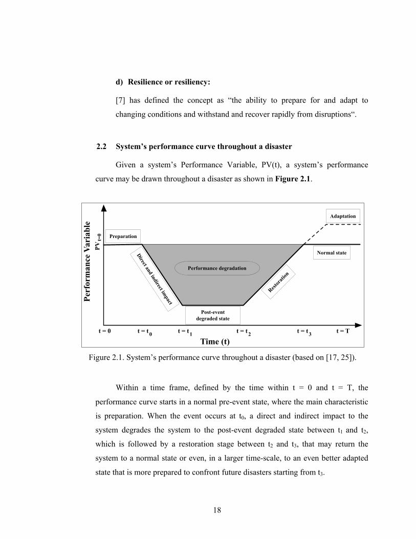
2.2 System’s performance curve throughout a disaster
Given a system’s Performance Variable, PV(t), a system’s performance
curve may be drawn throughout a disaster as shown in Figure 2.1.
Figure 2.1. System’s performance curve throughout a disaster (based on [17, 25]).
Within a time frame, defined by the time within t = 0 and t = T, the
performance curve starts in a normal pre-event state, where the main characteristic
is preparation. When the event occurs at t0, a direct and indirect impact to the
system degrades the system to the post-event degraded state between t1 and t2,
which is followed by a restoration stage between t2 and t3, that may return the
system to a normal state or even, in a larger time-scale, to an even better adapted
state that is more prepared to confront future disasters starting from t3.
Time (t)
Perf
orm
ance
Var
iabl
e
t = 0
PV
t=
0
t = t0 t = t1 t = t2 t = t3 t = T
Performance degradation
Preparation
Direct and indirect impact
Post-event degraded state
Restor
ation
Normal state
Adaptation

19
2.3 Electric power system’s structure
Electric power systems are complex interconnected systems that are divided
in three distinct segments: generation, transmission and distribution; a simple
network presented in Figure 2.2 illustrates this segmentation, present in this study.
Currently, the development of new technologies is making power systems more
complex by evolving to the smart grid concept.
The electricity generation is carried out by power plants (1) that may use a
wide range of resources (e.g. solar irradiance, water, oil, wind and coal) to produce
energy with different technologies. This is done at a medium voltage level and
connected to a local substation (2), which constitutes a node of the network.
The transmission segment starts at the substation (2) where voltage levels are
increased in order to diminish losses, while it is being transported in transmission
lines supported by towers (3) to another substation (5) in a different location where
it is transformed to a medium or low voltage.
The distribution segment starts at the substations (5), where voltage may be
transformed to a low level to supply residential consumers (7) or may be kept at
medium level to supply industrial consumers (4,6), which depending on the size
could also be connected directly to the transmission segment (4).
Figure 2.2. Electric power system’s structure (adapted from [8]).
Generation segment Transmission segment
Distribution segment
(1)
(4)
(2)
(3)(3) (5)
(6)
(7)

20
The main components considered in the diagram and in this study are power
plants, towers, transmission lines, substations and consumers (or loads).
Power plants are composed of generation units, which are characterized by a
number of technical parameters, such as their installed capacity, net (minus own
consumption) active/reactive maximum/minimum generation, start-up times,
variable costs, among others. Towers are vital components that support overhead
power conductors, which are able to transport electricity constrained to their
thermal capacity. Substations are facilities that are able to change the voltage from
one level to another (with transformers), regulate the voltage, convert AC to DC
and vice versa if required and is where safety/protection devices are installed, such
as disconnect switches, circuit breakers, lightning arresters, etc. Loads are usually
classified in industrial, commercial and residential consumers and represent the
demand of the system.
2.4 Types of risk analyses
Various system evaluations may be performed depending in what is
included. As it is shown in Figure 2.3, in this work, a classification of four types
of system analyses is proposed depending in what studies are included:
a) Single-phase analysis:
Commonly, because of the complexity of the problem, researchers have
gone deep into the understanding of the threat (e.g. [9]), the development of
fragility studies of components (e.g. [10]), models and tools to understand
the operation of electric power systems (e.g. [11]) and models to manage and
optimize system’s restoration (e.g. [12]). These stages and their complexities
are explained in more detail in Chapter 4. Even though these approaches
might be useful, an integral point of view can result in a better understanding
of the whole problem.

21
b) System fragility analysis:
Some authors have integrated the threat analysis and the system topology.
This system fragility analysis enables to understand the capacity post
disaster of the system after a disastrous event by identifying which
components will commonly fail and which may continue working (e.g. [13]).
c) System serviceability analysis:
Research groups have integrated in a single study the threat study, the
system topology and the system operation. When this is carried out, it may
be considered as a serviceability analysis. This permits to know the actual
capacity of the system to supply the demand over a time frame (e.g. [14]).
d) System resilience analysis:
In the past few years, a number of authors have started to integrate the threat
characterization, the system topology, the system operation and also the
system restoration. This analysis is the most complete study and the
approach taken in the present research (e.g. [15-18]).
Figure 2.3. Types of system risk analyses (own elaboration).

22
3. STATE OF THE ART AND CONTRIBUTIONS OF THIS THESIS
Electrical power systems have been designed and operated to be reliable against
abnormal but foreseeable contingencies. The concept of reliability3, defined as the
ability to supply adequate electric service on a nearly continuous basis, with very few
interruptions over an extended time period [19], has been extensively applied in the
electric sector. However, dealing with unexpected and less frequent severe situations
remains a challenge.
Resilience is an emerging concept and, as such, it has not yet been adequately
explored in spite of its growing interest, particularly in power systems where there are
almost no publications on the matter in IEEE periodicals [15, 21].
This chapter aims at explaining different perspectives researchers from the power
systems community have taken to analyse this problem. Then different methodological
advances in the topic are presented and finally the contributions of this thesis are listed.
3.1 Different perspectives for the resilience concept
In 2014, the third number of the periodical IEEE Power and Energy
Magazine covered the resilience concept with the title “Surviving with resiliency“.
The same year, CIGRE released the report “Disaster recovery within a CIGRE
Strategic framework: network, resilience, trends and areas of future work”. This
reflects the fact that resilience has become a major topic in the area. However,
there is no consensus on how to treat the concept.
Given the complexity of the problem and the system, it is understandable
that different perspectives are taken. For example, within the mentioned IEEE PES
Magazine issue, Article [22] is centred in how microgrids can enhance the
resilience of the European megagrid. Here resilience is treated in a dynamic time
frame, where microgrids can help specifically in the islanding and restoration
3 Internationally, its main features are adequacy and security [19]. In the Chilean technic normative quality of service is included as a third feature [20].

23
procedures. Article [23] focuses on the same issue and methodology, giving as
example the microgrids developed in Japan. Article [24] discusses how does an
integrated lightning system in a smart city improve resilience by strengthening the
mesh and adding redundancy. Two more articles, describe projects where different
strategies are being used, such as hardening the system components, the
deployment of microgrids as well as distributed and renewable generation devices
and the automation of the system.
With the exception of Article [25], none of the above articles have developed
an analysis of the system throughout the disaster in all of its stages. As [26]
suggests “a standardized definition of resiliency is needed to develop the
requirements and procedures for (..) system planning and operation”.
3.2 Methodological advances of resilience assessment and adaptation in
electric power systems
There are a few works related to power systems that take as base the curve in
Figure 2.1 and have a system perspective. Nevertheless, studies published in other
fields are briefly described below.
For instance, in [16], a joint effort of European universities analyses the
impact of earthquakes on various cities and different critical infrastructures,
including the power systems of Sicily. This study included the use of fragility
curves and an object-oriented programming to assess the pre- and post-disaster
performance of the network.
In [15], the impact of windstorms is analysed using wind fragility curves,
running DC optimal power flows on the IEEE-6 bus reliability test system and
comparing different adaptation cases.
The resilience of the electric system of Harris County, Texas, US, is
evaluated in [17] by running four models: hurricane hazard model, components
fragility model, power system response model and restoration model. The results
are classified in technical, organizational and social dimensions of resilience.

24
In [18], micro-components of the transmission network under seismic stress
are modelled to assess the resilience of the power system in Los Angeles, US. The
vulnerability is also modelled, with fragility curves and risk curves developed as
results.
Another notable effort, that has involved software developments, is Hazus,
from the Federal Emergency Management Agency (FEMA) [27]. This platform
has developed various fragility curves with damage states for many systems, some
of them used in this research.
Even though the recent work on the topic has been a huge step towards
understanding and measuring resilience, further research in this area remains a
concerning issue given the consequences of these and other catastrophic threats to
different systems around the world.
3.3 Contributions of the present work
The contributions of the present work are listed below:
An integral analysis with a system perspective covering the whole
disaster process is carried out to confront the problem of natural disasters
and electric power systems. It is common to find in literature that researchers
studying disaster management and power systems choose single-phase approaches
where the intention is limited to individual elements at risk.
A novel multi-phase resilience assessment and adaptation framework is
formalized by identifying the best practices in recent international literature.
Three different natural hazards and two electric power systems are
modelled to apply the resilience framework presented. Therefore, comparisons
are possible. In all publications found about the topic, only a single hazard and
system is modelled.
The test systems are representative of national grids with focus on the
generation and transmission system, where potential impacts are wider, but

25
with fewer details. In most publications the test system is focused on the
distribution level, losing a national perspective and being unable to apply national
strategies.
Multi-disciplinary work was carried out, with people from public and
private organizations and from different countries. Due to the complexity of
resilience studies, different fields have to be involved to be able to cover the whole
process.

26
4. MULTI-PHASE RESILIENCE ASSESSMENT AND
ADAPTATION FRAMEWORK
In this chapter, the resilience and adaptation framework presented in Figure 4.1,
and given in detail in Appendix B, is proposed for evaluating the impact of natural
disasters on the resilience of electric power systems4 and the effect of possible
adaptation strategies. This framework is presented next.
Figure 4.1. The multi-phase resilience and adaptation framework (own elaboration).
4.1 Multi-phase resilience assessment
The resilience assessment consists of four phases: threat characterization,
fragility of the system’s components, the reaction of the system and finally its
restoration.
4 Even though the resilience framework proposed can be extended to study any threat and any critical infrastructure, the study focuses in power systems so the phases do not incorporate aspects that may be of importance to other systems.

27
4.1.1 Phase one: threat characterization
The objective of this phase is to model the magnitude, probability of
occurrence and spatiotemporal profile of a hazard. To this end, the causes, physical
aspects and consequences of the threat must be understood. Two approaches can
be taken, one is to build deterministic scenarios, where historic events are
modelled, and the other one is to build probabilistic scenarios, where potential
future scenarios are projected.
For deterministic modelling, depending on the natural hazard under
investigation, different tools can be used. For extreme weather events, generally
the weather database needed may be acquired through Climate Models (CM),
which can model the threat with a certain geographic and time resolution, or using
real measurements with time and geographic features from weather stations. In the
case of seismic and tsunami hazards seismographs and sea-level measurements
database should be used.
For probabilistic scenarios, different projection methods can be used. The
selected method has to be suitable to be applied to the specific event (e.g.
earthquakes, tsunamis, floods, etc.) and be able to make an estimate of anticipated
forces, possibly much greater than have ever been observed, using historical or
model-generated data. For the case of data generated by CM, parametric studies
are useful, where the parameters are modified by a certain factor (usually taking in
consideration real extreme measurements or expert knowledge). For the case of
instrumentally measured data, a first option is Power Law, which has modelled
numerous natural phenomena, such as the Gutenberg-Richter number-size
distribution of earthquake magnitude and other probabilistic predictions of data
behaviour [28]. Specifically for earthquakes, as developed by [29] and explained in
[30], each seismic source has an annual amount of earthquakes that exceeds a
given magnitude, which is represented by Equation 4.1.

28
!"#!" !! ! !!!= !!!!! − !" (4.1)
Where !! ! is the mean annual frequency of the seismic events that
exceeds magnitude m, and coefficients a and b are estimated by regressions of past
events. Given lower and upped bound magnitudes Mmin and Mmax, respectively, the
cumulative distribution function (CDF) of the magnitude of an earthquake
!!"# ≤ ! ≤ !!"# is presented in Equation 4.2 and its probability density
function is presented in Equation 4.3.
!! ! = ! ! ≤ ! = ! !!!"!!(!!!!"#)
!!!"!!(!!"#!!!"#!) (4.2)
!! ! = ! ! = ! = ! !∗!" !" ∗!"!!(!!!!"#)
!!!"!!(!!"#!!!"#!) (4.3)
A second option for instrumentally measured data, is Extreme Value Theory
(EVT) [31], which is based on the distribution of the maximums (or minimums) by
defining a return period T (e.g. 100-years) and estimating its return value X(T) (e.g.
60 mm). This would mean that an event of X(T) is estimated to happen every T
years. EVT has two main approaches: Block Maxima Approach (BMA) and Peaks
Over Threshold (POT). Both approaches have the aim of estimating X(T) for rare
extreme events. In the case of BMA, this is done by a parametric modelling of
maximums (or minimums) taken from large blocks of independent data. In the case
of POT, this is done by a parametric modelling of independent exceedances above
a large (or low) threshold. Both approaches then use the Generalized Extreme
Value (GEV) distribution [32, 33]. GEV has the flexibility of combining the three
types of extreme distributions, namely Type I-Gumbel, Type II-Fréchet and Type
III-Weibull. GEV’s cumulative distribution function (CDF) is as follows:

29
! !;!,!, ! !!!!= !!!!!!(!!!!!!!! )!
!! !!!!!!!!!, !"#!1+ !(!!!)
! > 0 (4.4)
In Equation 4.4, ! (location), ! (scale) and ! (shape) are the three main
parameters of GEV. The particular cases of ! = 0, ! > 0 and ! < 0 are respectively
equivalent to the distributions Type I, whose tails decrease exponentially; Type II,
whose tails decrease as a polynomial and Type III, whose tails are finite. When the
parameters are estimated to fit the dataset, a projection diagram can be drawn to
visualize the return periods and return values [34].
4.1.2 Phase two: vulnerability of system’s components
The aim of this phase is to determine the damage level of each component of
the system. To do this, the following three steps are considered:
i. identify the vulnerable components
ii. fragility modelling of the components
iii. assign damage states
In the first step, the components identified are those that are vulnerable to
the threat that could possibly have a high impact on the network resilience. Also,
the type of component must be selected. In electric power systems, components
can be classified in macro or micro components [16]. For example,
high/medium/low voltage substations/power plants, distributions circuits,
transmission towers and lines can be classified as macro components. Circuit
breakers, transformers, lightning arresters, switches and all those elements that
describe the internal logic of macro components are micro components. The use of
one or another depends on the objectives of the resilience study being undertaken.
Some studies also propose modelling people and communities from a physiologic
perspective [35, 36].

30
The second step corresponds to modelling the fragility of the components to
the natural threats. The concept of Fragility Curves has its origins as a structural
reliability concept [37, 38], and is a useful tool for a stand-alone analysis of each
component. A fragility curve, as shown in Figure 4.2, expresses the probability of
failure of a component conditioned on the impact of the hazard. In practice, these
failure probabilities are compared with a uniformly distributed random number
r~U(0,1). If the failure probability of the component is larger than r, then the
component fails.
Figure 4.2. Generic fragility curve: probability of failure (%) vs threat parameter (own elaboration).
It is important to note that a “failure“ of the component does not necessarily
imply a complete collapse of the component (i.e. removal from service). For
example, after a seismic event a power plant that is composed of more than one
generation unit might have just a portion of the units out of service, meaning that
the power plant will be able to work at a degraded maximum generation capacity.
At the same time, other components such as transmission lines have a binary
damage state: tripped or non-tripped.
Thus, as a third step, the damage state of the components must be addressed.
In order to do this, two approaches can be used as shown in Figure 4.3, where (a)
uses different fragility curves for different damage levels (as used by [27] and

31
Chapter 6) and (b) relates the damage level to the zone of the fragility curve
defined by percentiles (as used in Chapter 5).
Particularly for electric power systems, even though, most frequent faults
happen at a distribution level, less common but with a higher impact occur at a
transmission and generation level. Because of this, and to be able to have a nation-
wide perspective of resilience this research focuses on the generation and
transmission level components.
Figure 4.3 (a). Different fragility curves to assign damage states. (b). Different zones in
the fragility curve to assign damage states. (Own elaboration).
4.1.3 Phase three: system’s reaction
The objective of the third phase is to evaluate the performance of the critical
infrastructure when it is exposed to the extreme event. In electrical power systems,
to do this, numerous evaluation tools have been developed over the last decades;
such as the CASCADE model, which studies the cascading mechanism of a
blackout [39]; the ORNL-PSERC-Alaska (OPA) model, which is based on a DC
optimal power flow and it is built upon Self-Organized Criticality [40, 41]; the
Hidden Failure model, which is based on approximated DC power flow and
standard linear programming optimization of generation redispatch to represent
hidden failures of the protection system [42]; and the Manchester model, which is

32
built upon AC power flow, uses load shedding and a power flow solution to
determine the power system operation [43-45].
When modelling the impact of extreme natural events, it is important to take
into account the diverse impact of the weather front or geographic profile moving
across the system, which is both spatial- and temporal-dependent. The resilience
model used in this phase should thus be capable of capturing the spatiotemporal
stochastic impact of the natural disaster on the resilience of power systems. It has
to consider the flexibility of the system given by the installed technology and
possible international interconnections. It should also be capable of providing a
component and area criticality index, which will enable the resilience enhancement
of the most vulnerable components. Furthermore, following the disaster, it is very
likely that the system will be divided into multiple islands, which should be
incorporated in the impact assessment model.
4.1.4 Phase four: system’s restoration
The response to the disaster and the restoration times following the disaster
are strongly related to the following three aspects:
i. damage caused
ii. amount of human and material resources available
iii. accessibility of the affected area.
The restoration process can only be undertaken under the condition that both
repair-teams and spare parts are available. The fast restoration and recovery of
critical infrastructure is a crucial feature of resilience (as discussed in Chapter 2).
Therefore, proper and effective emergency and restoration strategies should be in
place to restore the system to its pre-disaster state as fast as possible.
4.2 Multi-phase adaptation strategies
The probability of extreme weather events is relatively low, but their impact
is so high that is vitally important to enhance the resilience of critical

33
infrastructures. Particularly, for electric power systems, this can be achieved
through a wide range of short- and long-term measures. Short-term measures are
discussed in detail in [25, 46]. Long-term measures can be grouped in strategic
adaptation cases that improve specific phases of the resilience of the system.
Namely, the cases are: (i) Normal, which is the basic network; (ii) Robust, that
improves the resistance of the system; (iii) Redundant, which includes backup
installations or spare capacity enabling the diversion of the power flows to
alternative paths of the network; and (iv) Responsive, that enables a faster
response from the disruptive events. It can thus be seen that these adaptation case
studies can improve, respectively, the 2nd, 3rd and 4th phases of the resilience
framework.
Figure 4.4 (a). Normal case. (b). Robust case. (c). Redundant case. (d). Responsive case.
(Own elaboration. Numbers indicate mean time to repair).
Explicative diagrams of the adaptation cases are presented in Figure 4.4
(based on the examples in [47]), where (a) represents the normal network, which
consists of four nodes and three links with their mean times to repair, (b)
represents the robust case, having more resistant links that can be interpreted as a
shift of the fragility curve. (c) shows the redundant case including alternative paths
and (d) is the responsive case, where the mean times to repair are decreased.

34
4.3 Resilience metrics
Depending on the aim of the resilience study, the performance of electric
power systems can be measured using numerous different metrics. Two
measurements that are able to describe the impact of the extreme event within a
time frame are the Expected Energy Not Supplied (EENS) and the Energy Index of
Unreliability (EIU) [19, 48]. The first, shown in Equation 4.5, indicates how much
service (energy) was not provided during the studied time period as an absolute
number (MWh or GWh). The second, shown in Equation 4.6, is directly related to
EENS, which is normalized using the total energy demand in the studied time
frame (%). In the following equations, !! is the energy not supplied with a
probability !! of occurrence of scenario k during the time frame of the study. E
represents the energy demand in the whole study period.
!!"#! !"ℎ !!= !!!! !! ∗ !!!!!
!!!! (4.5)
!"#! % !!= !!!!!!"#! !∗ 100%!!!!!!!! (4.6)
4.4 Resilience modelling
In the previous sections of this chapter, the framework concepts have been
explained. In Figure 4.5, a flow chart of the resilience framework is displayed.
The model is based on Sequential Monte Carlo Simulations, where every grey box
represents one scenario and within every scenario an hourly sequential simulation
is run. It has to be noted that the applications in following chapters may differ from
the present flow chart.

35
Figure 4.5. Resilience modelling flow chart (own elaboration).
hour = 1…Nhours
scenario = s
Initialization of parameters Hourly power and reactive demand per bus.
Hazard scenarioApply deterministic or probabilistic method for event.
Hazard hourly scenarioHourly intensity measure of event in every component site (e.g. wind speed, peak ground acceleration, etc).
Read inputs Load system case (lines, buses, generators).Set Nhours, Initial component damage states, initial operation state of units.Set ENS to 0.
Impact on componentsRun fragility curve analyses for every component.Assign damage states.
Resilience metricsENS = ENS + Energy not supplied this hour.
System operationSet operation state of the system (emergency and normal).Island handling.With online components run OPF of this hour.
Restoration of componentsFor all components:
Subject to human and resources availability, event intensity and damage state assign time to repair.
Is time to repair < hour
Is component damaged?
Component damage state = normal.
no
yes
yes
36
5. APPLICATION TO WINDSTORMS AND FLOODS IN GREAT
BRITAIN
In the present chapter, the multi-phase resilience framework previously presented
is illustrated by assessing the impact of potential future scenarios of windstorms and
floods on a reduced version of the Great Britain’s electric power system as it is
explained hereafter.
5.1 Influence of extreme weather and climate change in Great Britain’s
power system
In this Section, extreme weather events are described along with the
influence of climate change and possible future scenario hazards.
5.1.1 Extreme weather events
A disruptive weather event can be classified into small, moderate, serious,
major and extreme based on the number of customers disconnected, the duration
and frequency [49]. For example, in the USA, extreme weather-related events
account approximately for 80% of the large-scale power outages from 2003 to
2012 [50], with the annual impact ranging from $20 to $55 billion [51].
Great Britain, in particular, is significantly affected by weather-related
power outages. In [52], it is reported that only from April 2008 to March 2009, 211
faults occurred on the transmission network in England and Wales and other 44 in
Scotland, of which 23% and 95% were caused by weather, respectively. These
weather-related faults can be categorized in one of eight causes: wind and gale;
snow; sleet and blizzard; lightnings; ice; freezing fog and frost; heat waves;
flooding and rain [52, 53]. For example, several transmission substations and
power stations are at high risk of flooding, while high winds can cause
transmission lines and towers to collapse. Also, in 2007, Great Britain suffered the

37
wettest summer in its history. This produced extreme rainfall compressed into
short periods of time that caused a series of destructive floods catalogued as the
country’s “largest peacetime emergency since World War II“ [54]. Moreover, a
few years later in 2014, an even more extreme weather-year took place. As
described by the National Meteorological Office (MET), this was the wettest, 5th
warmest and probably most disastrous winter in the UK [55]. Consequently, the
Climate Change act of 2008 required the UK electricity industry to report on
adaptation measures to deal with the effects of weather and the effect of climate
change [56]. This motivates to analyse particularly windstorms and floods in this
research.
5.1.2 Climate change and future hazard scenarios
In 1992, the United Nations Framework Convention on Climate Change
(UNFCCC) was created with the objective to “stabilize greenhouse gas
concentrations in the atmosphere at a level that would prevent dangerous
anthropogenic interface with the climate system“ [2]. To achieve this, the
Intergovernmental Panel on Climate Change (IPCC) supports UNFCCC producing
reports of the scientific, technical and socio-economic aspects of global warming
with its potential impacts and options for adaptation and mitigation. Until today, a
series of five comprehensive reports have been published. The latest one, in 2014,
stated that now, the IPCC, is “95% certain that humans are the main cause of
current global warming“ and that “climate change will amplify existing risks and
create new risks for natural and human systems“ [2]. Even though, mitigation of
Greenhouse Gases (GHG) is crucial to constrain climate change, adaptation of
infrastructure becomes essential, before mitigation measures can have any effect
[57]. In consequence, possible future changes in natural hazards must be analysed.
According to the IPCC, climate change projections may vary from region to
region, but generally it is likely that wet and dry extremes are going to become

38
more severe [2]. In Great Britain, particularly for the variables studied here, reports
indicate that while wind has a high uncertainty on how it will change [52], flood
risk will escalate because of the potential increase of rainfall volume and intensity
[58]. Unfortunately, quantitative studies disagree on how will they scale up [52].
5.2 The Great Britain’s simplified electric power system
The Great Britain network used in this study is a simplification5 of the real
one at the end of 2010 [59]. As it is shown in Figure 5.1 (a), the grid consists of 29
nodes, 98 overhead transmission lines in double circuit configuration and one
single circuit transmission line between nodes 2 and 3, and 65 generators (with
81.5 GW of installed capacity) which are located at 24 nodes and include several
technologies, such as wind, nuclear and CCGT.
Figure 5.1 (a). Great Britain’s simplified system. (b). Weather regionalization of the
system. (Own elaboration with M. Panteli).
5 The components are not real; they represent a group of real components while trying to replicate the real AC power flows and operation of the actual system.
26
27
25
2829
23
1822 21
20
1917
16141312
11 15
109
87
65
4
3
1 2
24
NodesTransmission route – double circuit OHL
Transmission route – single circuit OHL
26
27
25
2829
23
1822 21
20
1917
16141312
11 15
109
87
65
4
3
1 2
24
1 2
4
5
6
Weather Region
3

39
Interconnections with external subsystems, i.e., France, the Netherlands and
Northern Ireland are included. The demand, plotted in Figure 5.2, represents the
winter peak week in 2010.
Figure 5.2. Winter peak demand week in Great Britain (Own elaboration).
5.3 Resilience assessment
The resilience of the test network is evaluated against windstorms and
floods, which constitute severe threats to the Great Britain system.
5.3.1 Phase one: windstorms and floods characterization
As explained in detail in Section 4.1.1, the threat characterization phase aims
at defining the event’s probability of occurrence, magnitude and spatio-temporal
profile. Therefore, in order to account for the spatial feature of the weather events,
the “big island” is divided into 6 weather regions, as shown in Figure 5.1 (b).
Weather conditions are assumed to be homogeneous within each region, so the
0
5000
10000
15000
20000
25000
30000
35000
40000
45000
50000
0
5000
10000
15000
20000
25000
30000
35000
40000
45000
50000
1 8 15 22 29 36 43 50 57 64 71 78 85 92 99 106 113 120 127 134 141 148 155 162
Rea
ctiv
e po
wer
dem
and
[MVA
r]
Act
ive
pow
er d
eman
d [M
W]
Time [hour]
Active power Reactive power

40
fragility of each component is conditioned to the same stress across each weather
region. Potential future scenarios were modelled as explained hereafter.
For the windstorms modelling, the main characteristic is the geographic
mapping of the location and magnitude of wind speed. Therefore, hourly mean
wind data for 33 years (1979-2011) was obtained using MERRA re-analysis [60].
On the other hand, floods are more complex and affected by many factors, such as
the capacity of drainage system, saturated ground, high river levels and
accumulated rainfall. But in general, especially river and groundwater floods are
strongly related to rainfall. For example, in [61] flood is linked directly to
accumulated rainfall. The hourly rainfall data for the same years, i.e., 1979-2011,
was obtained from more than 17000 rain gauge stations all over Great Britain in
that time frame, which was provided by the MET Office, UK [62]. This analysis
altogether provides the temporal characterization of the threats: 33 years of wind
and rainfall profiles with hourly resolution.
In order to deal with the uncertainty associated with the future weather
conditions as a direct impact of climate change, five scenarios have been
developed for evaluating the impact of windstorms, floods and both hazards
together.
Given that wind speed was taken from a Climate Model, where the focus is
on average measurements (with a maximum average of approximately 20 m/s), one
suitable approach to use in order to model extreme winds that can damage the
transmission components is to parametrically scale up the wind profiles. Therefore,
the winds profiles of the 6 weather regions have been scaled up using a
multiplication factor in the range {1,3} in steps of 0.5, resulting in five windstorms
scenarios (meaning that x2 and x3 would represent approximately wind speeds of
40 m/s and 60 m/s, respectively). The wind profile is scaled up by the same factor
in the whole network, so the impact affects the entire network instead of specific
areas.

41
For floods, given that the rainfall data was taken from real measurements,
five levels were modelled by applying extreme value theory. Assuming the data is
independent and identically distributed, the Block Maxima Approach (BMA) and
the Generalized Extreme Value (GEV) distribution was used. Then the parameters
of the GEV distribution were estimated to fit the dataset and a projection diagram
was drawn for each region. An example of a projection diagram for Region 4 is
shown in Figure 5.3.
Figure 5.3. Projection diagram for Region 4 - horizontal axis in logarithmic scale - (own
elaboration).
Thereafter, five return periods were chosen (i.e. 10-year, 33-year, 100-year,
150-year and 250-year), which provided five return values for the peak rainfall
within one hour for every region. For example, for Region 4 the return values
projected were: 17 mm, 32.9 mm, 59.7 mm, 74.1 mm and 97 mm, respectively
(which is reasonable taking into account that the highest hourly rainfall recorded
by Met Office was 92 mm in 1901 [63]). Then, rainfall scale parameters are
calculated with Equation 5.1, where given a return period λ-year, the scale
parameter, π γ, ρ, λ , for the year γ and region ρ is equal to the return value Τ (!-
year) [mm] divided by the peak rainfall value of the year γ in the region ρ, Ρ (γ, ρ)
[mm].

42
! !,!, ! !!!!= !!!! !!(!!!"#$)!!(!,!) !!!!!!!!! , !"#!! ∈ [1979, . . ,2011] (5.1)
5.3.2 Phase two: fragility of electrical components
As detailed in Section 4.1.2, the component’s fragility phase should follow
three steps: first identify the vulnerable components, then use a fragility curve
approach and finally assign damage states. Therefore, in the Great Britain study
case, the key vulnerable macro components shown in Table 5.1 were identified
and modelled.
Table 5.1. Threats analysed with their correspondent key vulnerable components identified (own elaboration).
Threat Vulnerable components Wind Storms Transmission lines Transmission towers
Floods Substations Power plants
Subsequently, the vulnerability of each identified component is analysed
through fragility curves. Used lines and towers’ wind fragility curves are presented
in Figure 5.4.(a) [15]. Likewise, in Figure 5.4.(b), the flood fragility curves used
are shown. Floods are strongly related to the accumulated rainfall, which can be
produced by an intense short event (less than three hours) or a prolonged event
(less than ten hours). These implicate that beginning with rainfalls of
approximately 20 mm/hour for at least three hours, the risks of flooding exist [64].
Also, to take into account the particularities of power stations and substations,
when a flood occurs, a probabilistic assignation is done (i.e. 38% for power plants
and 33% for substations) based on a report that classifies the flood risk of power
plants and substations [65] (this means that 38% of the power plants flooded will
actually fail). Therefore, in the case of floods, the component’s risk profile and the
floods fragility is jointly used. The accuracy of these curves can vary depending on
the particularities of each component. Consequently the accuracy of the assessment

43
can be improved in further works by improving the methods to generate the
fragility curves.
Figure 5.4. (a) Lines and tower’s fragility curves ([15]). (b) Floods by intense or prolonged rainfall fragility curves (own elaboration with data from [64]).
Because some lines pass across multiple areas experiencing different
weather conditions at each region assumptions had to be incorporated to model
this. In the case of lines, the highest line failure probability among the regions is
used for the whole line. In the case of towers, which are considered to be every 300
meters across lines, a percentage of the line’s length in each region is assumed for
estimating the number of towers in every region. The aggregated failure
probability of all towers supporting a line is then used to estimate the line failure
probability due to a tower collapse.
Finally, following the failure of a component, the damage state has to be
assigned. The approach in this study is to establish the damage through zones in
the fragility curve as shown in Figure 4.3. (b). For example, power plants have
four possible damage states: minor, moderate, extensive and complete. These
states are determined by the percentiles 0-25th, 25th-50th, 50th-75th and 75th-100th,
respectively. Lines, towers and substation’s potential damage are modelled with
two states: operative and non-operative.

44
5.3.3 Phase three: power system’s reaction
As detailed in Section 4.1.3, the system’s operation phase consists in
Sequential Monte Carlo Simulations with hourly OPF analyses. Also, in order to
capture the spatiotemporal impact of the wind and rainfall fronts moving across the
transmission network, a Sequential Monte Carlo-based time-series simulation
model has been developed. This enables the representation of the weather and
electrical events in a chronological order as they happen in reality at different
locations of the test system. An hourly simulation step is used, which is considered
sufficient for modelling weather events. However, any time resolution can be used
if desired and provided that the relevant information is available, e.g., weather
profile. Further, one winter week is used as a simulation period, where extreme
wind and rainfall events are expected considering that severe weather events do not
usually last longer in Great Britain.
At every simulation step, the wind- and rainfall-affected failure probabilities
of the electrical components obtained by the fragility curves are fed to the time-
series simulation model as explained in the previous phases. Following this
approach, the real-time weather-adjusted operation state of each electrical
component is obtained. An AC Optimal Power Flow (OPF) is used for assessing
the performance of the test network at every simulation step, which helps
determine if load shedding is required for stabilizing the system. For solving the
power flows the Newton method was used, and for the optimization problem
Matlab Interior Point Solver (MIPS) was employed. Finally, following a severe
disturbance, the model is also capable of detecting islanded nodes and operating
them independently until they are reconnected, which is very important when
studying high impact events that can produce the network to be separated in many
disconnected islands. It has to be noted that this does not refer to the studies related
to controlled islanding of power systems during disturbances.

45
5.3.4 Phase four: power system’s restoration
As explained in Section 4.1.4, three aspects should be taken into
consideration for the components restoration: damage caused, human and material
resources availability and the accessibility to the affected area. In this study, for
simplicity reasons, the restoration curves are only related to the difficulties of the
repair crew to enter the affected areas. The component restoration curves are
defined by exponentially distributed curves with mean parameters as shown in
Table 5.2. A Mean Time To Repair (MTTR) of 10 hrs and 50 hrs is assumed for
lines and towers respectively, and 10 hrs and 30 hrs for power plants and
substations respectively (referred to as MTTRbase). The weather intensity is
classified here as follows: for windstorms, it can be Low (less than 20 m/s),
Moderate (between 20 m/s and 40 m/s) or High (more than 40 m/s), while for
floods it can be Low (less than 138 mm for intense accumulated rainfall or 280
mm for prolonged accumulated rainfall or High (more than 138 mm for intense
accumulated rainfall or 280 mm for prolonged accumulated rainfall). As weather
intensity increases, the repair crews need more time to enter the affected area and
restore the damaged components, which is modelled here as a random increase in
MTTRbase as can be seen in Table 5.2.
Table 5.2. Mean times to repair (hours) for different weather intensities (own elaboration).
Threat Component MTTR for different weather intensities
(Wind speed (m/s) / Accumulated rainfall (mm)) Low Moderate High
Windstorms Lines MTTRbase MTTRbase×rand[2,4] MTTRbase×rand[5,7]
Towers MTTRbase MTTRbase×rand[2,4] MTTRbase×rand[5,7]
Floods Power Plants MTTRbase --- MTTRbase×2 Substations MTTRbase --- MTTRbase×2

46
5.4 Resilience adaptation
In this study, the adaptation strategies discussed in Section 4.2 are applied to
the critical transmission route shown in Figure 5.5 from North to South Great
Britain. Following power flow studies (mainly focusing on the maximum power
flows on the transmission lines), this corridor was identified as one of the critical
transmission routes for preserving the resilience of the entire power system.
Particularly, for the normal case, the basic network was used with no
resilience enhancement. For the robust strategy case, the fragility curves of the
components (see Figure 5.4) in the critical path were shifted to the right a 15% of
the 50th percentile of the curve. For the redundant strategy case, identical parallel
lines have been added to the critical transmission path. Finally, for the responsive
strategy case, the mean times to repair of the components in the critical path were
supposed unaffected by the severity of the weather.
Figure 5.5. Dotted lines show the critical transmission corridor for which the adaptation case studies are applied (own elaboration with M. Panteli).
26
27
25
2829
23
1822 21
20
1917
16141312
11 15
109
87
65
4
3
1 2
24
47
5.5 Results and discussion
The impact of windstorms and floods is first modelled independently, and
then the combined impact of these threats is evaluated. In Figure 5.6, the
comparison between these single and multi-hazards is represented using EENS for
different intensities of the weather hazards. Where the impact increases with the
intensity of the event and the combination of hazards is much more severe than the
single threats. The impact of floods is greater than the windstorms mainly because
the substations affected by floods are more important to the network than other
components.
Figure 5.6. EENS [GWh/week] of different hazards in potential future scenarios (own elaboration).
Then, the EENS results for the strategic adaptation cases in the different
future scenarios are illustrated in Figure 5.7. (a) and (b), for windstorms and
floods, respectively. It can be seen that the best adaptation case for both hazards is
robustness, followed by responsiveness and finally redundancy, where for floods
this last strategic case has almost no improvement. This can be explained by the
different components each hazard has impact on, where windstorms affect lines
and towers, and floods affect power plants and substations. When the nodes of a
network (substations) are impacted, alternative paths are also affected; hence
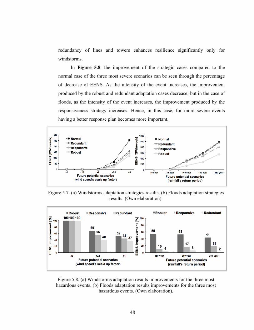
48
redundancy of lines and towers enhances resilience significantly only for
windstorms.
In Figure 5.8, the improvement of the strategic cases compared to the
normal case of the three most severe scenarios can be seen through the percentage
of decrease of EENS. As the intensity of the event increases, the improvement
produced by the robust and redundant adaptation cases decrease; but in the case of
floods, as the intensity of the event increases, the improvement produced by the
responsiveness strategy increases. Hence, in this case, for more severe events
having a better response plan becomes more important.
Figure 5.7. (a) Windstorms adaptation strategies results. (b) Floods adaptation strategies results. (Own elaboration).
Figure 5.8. (a) Windstorms adaptation results improvements for the three most hazardous events. (b) Floods adaptation results improvements for the three most
hazardous events. (Own elaboration).

49
Finally, in Table 5.3, the EIU results are presented. Here E, or total week-
demand, is equal to 7193 GWh. It can be seen that the EIU results are relatively
low except for the very extreme cases. This can be mainly due to the high
reliability of the test network. However, this low impact when expressed through
EENS or EIU can be very high in terms of financial losses, therefore a socio-
economic analysis should be performed to correctly assess the resilience of the
system and decide between different enhancement measures.
Table 5.3. EIU results (own elaboration).
Comparison of hazards in different scenarios
Scenarios Windstorms Floods Windstorms & Floods
10-year / x1 0.00% 0.00% 0.00%
33-year / x1.5 0.00% 0.32% 0.32%
100-year / x2 0.03% 4.50% 4.49%
150-year / x2.5 1.81% 8.22% 10.75%
250-year / x3 7.05% 13.67% 21.76%

50
6. APPLICATION TO EARTHQUAKES IN CHILE
Chile is a long and narrow country in South America with a population of around
18 million people6. It is a fast developing country, currently with a GDP per capita of
23,165 USD2014 (PPP)7 and a Human Development Index (HDI) of 0.828, which is
classified as very high. At the same time, it has seen its electric power installed capacity
grow 3 times between 1996 and 20129. However, this socio-economic growth is
challenged by the great amount and diverse natural threats, such as volcanic eruptions,
wildfires, droughts driven by climate change, floods, landslides, earthquakes and
tsunamis.
In this chapter, the influence of earthquakes and tsunamis in Chile is described,
focusing on earthquakes and electric power systems. Afterwards, the northern electric
power system modelled is presented and finally, the application of the resilience
framework is developed.
6.1 Influence of earthquakes and tsunamis in Chile
The strongest earthquake registered in modern history took place in
Valdivia, south of Chile, in 1960 with a magnitude of 9.5 Mw10. The most recent
mega earthquake in Chile, an 8.8 Mw magnitude event, struck the central zone
followed by a tsunami that hit the coastal areas on February 27, 2010. This
earthquake, ranked as the sixth-strongest recorded in modern history, produced a
loss estimated in US$30 billion equal to a 18% of the country’s GDP (more than
twenty times greater than the most disastrous event in the US until now: hurricane
Katrina in 2005) [66].
6 INE, 2014. 7 IMF, 2015. 8 UNDP, 2014. 9 Ministry of Energy of Chile, 2013. 10 Mistakenly called Richter magnitude. The Richter scale was succeeded by the Moment Magnitude Scale (MMS) in the 1970s and is currently broadly used around the world.

51
At the same time, Chile has been host to a significant number of tsunami
events. Three examples in the past five years are the large-scale tsunami of
February 27, 2010, witnessed throughout the national territory, the tsunami in the
north that struck Pisagua on April 1, 2014, after the same date earthquake
magnitude 8.2 Mw and while writing this thesis on September 16, 2015, a
subduction earthquake magnitude 8.4 Mw stroke nearby Illapel producing a
tsunami along the central coast (More detail is given in Appendix C). Also, due to
the geographical conditions in Chile, where the coast is closer to the earthquake
generation zone, the first wave arrival times are significantly short11.
These events highlight the need for research in this topic.
6.1.1 Influence of earthquakes in Chile’s power systems
As explained before, Chile has faced many critical hazards, where the
electric power systems have been tested. After the events on February 27, 2010,
which impacted the SIC, central system of Chile12, efforts to collect information on
how the system responded were carried out by [67-69].
Chile has a high standard of seismic requirements for its civil structures and
for its electrical components13. That is one of the main reasons why [67-69]
concluded that the electric power system responded well to the challenge
(nevertheless, with space for improvements). Their assessment of the segments of
the system that provides more than 93% of the national population is explained
hereafter.
11 For example during the 2010 and 2014 chilean tsunamis, wave arrival times were between 10 to 15 minutes following the seismic activity, while during Tohoku 2011, Japan, the first wave arrival times were between 30 to 40 minutes following the seismic activity (Cigiden, 2015). 12 Currently, Chile has two large interconnected systems and two small isolated systems. The first two are the northern (SING) and the central one (SIC). They are going to be interconnected in 2017. 13 The Chilean electric normative [20] indicates that high voltage facilities must fulfil the ETC 1.015 standard or the IEEE 693-1997 standard at “High Performance Level”.
52
a) Impact on generation
In February 2010, the installed capacity of the system14 was 11,023 MW
with a peak demand of 6,145 MW. At the time of the earthquake, the
dispatched generation was 4,522 MW. As a consequence of the seismic
event approximately 3,000 MW of generation capacity became unavailable
immediately after the event. In the following 30 days 2,257 MW were put
back into service and 693 MW remained out of service for up to six months
requiring major repairs.
b) Impact on transmission
Tanselec is the main transmission company in Chile with 8,239 km and 50
substations in the two main systems: SIC and SING. Transelec’s damage
assessment revealed that in the SIC 12 of the 46 substations and 1.6 km of
the 7,280 km of transmission lines suffered damages, representing 26% of
substations and 0.02% of transmission lines.
c) Impact on distribution
At the distribution level, most of the damage was detected. 4.5 million
people were affected by a blackout immediately after the event. However,
the electric components did not suffer from design or construction seismic
failures, but were mainly damaged because of nearby walls, landslides and
the tsunamis. CGED is the main distribution company that serves the most
affected area by the quake. The publications report that although 80% of the
clients were without supply the day after the event, this was reduced to 0.4%
two weeks later.
d) Operation and restoration
During the disaster, the country saw that one of the most weak critical
infrastructure systems was telecommunications. These problems produced
14 This “over capacity“ is due to the flexibility required by the system because of the high amount of hydro generation.

53
several difficulties to the operation and restoration of the electric power
system.
[68] explains that given the impacts on the electric segments just presented
the system operator had to plan the recovery in three stages. The first stage
was to restore service were no facilities were affected by forming islands. In
the particular case of the 2010 quake, the recovery experience started with a
five-island scheme, which later was integrated into a two island-scheme that
lasted for two days. The second stage consisted in the restoration of the
principal equipment with limited material and human resources. In 2010, the
efforts allowed the main transmission network to be restored to service in
less than 13 hours, albeit in a weakened condition – no N-1 conditions and
many breakers bypasses. The third stage, which took several months to
complete, had the responsibility to restore the reliability criteria to the
system.
One note that has been remarked is that the challenges from the generation
and transmission perspective were not as severe as in a typical blackout, because
the load demanded in the distribution level was reduced dramatically because of
the quake.
6.1.2 Future hazard scenarios in northern Chile
Since no major seismic event (> 8.5 Mw) has occurred in northern Chile
since the 1877 8.6 Mw megathrust earthquake that was followed by a huge tsunami,
the accumulation of elastic deformation is likely to be released in a future event
(which if released at once it could correspond to a 9 Mw earthquake). Figure 6.1
suggests that this area is a mature seismic gap with a high seismic and tsunami
hazard [70].
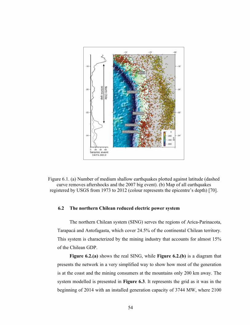
54
Figure 6.1. (a) Number of medium shallow earthquakes plotted against latitude (dashed curve removes aftershocks and the 2007 big event). (b) Map of all earthquakes
registered by USGS from 1973 to 2012 (colour represents the epicentre’s depth) [70].
6.2 The northern Chilean reduced electric power system
The northern Chilean system (SING) serves the regions of Arica-Parinacota,
Tarapacá and Antofagasta, which cover 24.5% of the continental Chilean territory.
This system is characterized by the mining industry that accounts for almost 15%
of the Chilean GDP.
Figure 6.2.(a) shows the real SING, while Figure 6.2.(b) is a diagram that
presents the network in a very simplified way to show how most of the generation
is at the coast and the mining consumers at the mountains only 200 km away. The
system modelled is presented in Figure 6.3. It represents the grid as it was in the
beginning of 2014 with an installed generation capacity of 3744 MW, where 2100
2 M. Metois et al.
Figure 1. Left-hand side: the solid curve depicts the number of Mw < 7 shallow earthquakes (depth < 60 km) plotted against latitude (0.2◦ sliding window).
Dashed curve: Aftershocks associated to the 1995, 2001, 2005 and 2007 Mw > 7 events removed. Right-hand side: map of all earthquakes registered by USGS
from 1973 to 2012 in North Chile. USGS catalogue is complete for Mw > 4.5 events in this region.
suggested that this area is a mature seismic gap with high seismicand tsunami hazard (Kelleher 1972; Nishenko 1991). In addition,the occurrence of recent intermediate magnitude earthquakes at theedges of this area potentially increased the stress on it. The 1995 Mw
8.1 Antofagasta earthquake (Ruegg et al. 1996; Delouis et al. 1997;Chlieh et al. 2004; Pritchard & Simons 2006) and the 2007 Mw
7.7 Tocopilla earthquakes (Delouis et al. 2009; Bejar-Pizarro et al.
2010; Peyrat et al. 2010) occurred South of the North Chilean gap,on both sides of the Mejillones peninsula (Fig. 2). The Arequipa2001 Mw 8.4 Peru earthquake ruptured North of the gap in the rup-ture zone of the 1868 megathrust earthquake (Perfettini 2005), andthe 2005, Mw 7.7 Tarapaca deep intraslab event affected its centralpart (Peyrat et al. 2006).
Nevertheless, the high seismic hazard associated to this gap maybe lower than anticipated. First, the rupture zone of the 1877 earth-quake is poorly known and this uncertainty makes the estimate ofthe seismic hazard in this area a real challenge (see discussion sec-tion). Secondly, part of the convergence between plates could havebeen accommodated by aseismic sliding on the interface since 1877,reducing the slip deficit. Therefore, it is important to measure theelastic strain above the subduction zone to quantify the locking de-gree on the subduction interface. Finally, in this part of the CentralAndes, the Altiplano develops, the mountain range widens and thebackarc subandean fold-and-thrust belt is an active structure whichseems also to accommodate part of the convergence between theNazca and South American plates reducing by so much the rateof accumulation on the subduction (McQuarrie 2002b; Arriagada
et al. 2008) (Fig. 2). However, whether or not this structure acts asthe eastern boundary for an Andean microplate behaving as a rigidblock, and to what extent it accommodates part of the total con-vergence, remain open questions. In North Chile, recent estimatesof backarc shortening rate vary from 5 to 15 mm yr−1 dependingon the authors (Norabuena et al. 1998; Bevis et al. 2001; Kendricket al. 2001; Brooks et al. 2003, 2011; Khazaradze 2003; Chliehet al. 2011). Actually, the long-term backarc shortening rate gradu-ally decreases from North to South (McQuarrie 2002a). Assessingthe seismic hazard on the trench in North Chile requires quantifica-tion of the partitioning of the convergence between both structures,since there is a large trade-off between the coupling amount on thesubduction interface and the Andean sliver block motion (Chliehet al. 2011).
Over the past two decades, international teams installed campaignand continuous Global Positioning System (GPS) networks in theregion to measure the interseismic deformation of the upper platenear the subduction zone (Ruegg et al. 1996; Norabuena et al. 1998;Bevis et al. 1999; Klotz et al. 2001; Khazaradze 2003; Chlieh et al.
2004). Unfortunately, these measurements were affected by severalproblems: each data set was published in an unknown singularreference frame, hence difficult to combine (Kendrick et al. 2001)and the networks were too sparse to give a good resolution ofthe coupling distribution on the interface and of the sliver motion.Moreover, these measurements contain co- and post-seismic signalsinduced by several Mw > 7 earthquakes in the North Chile area,introducing noise on the interseismic deformation. Recently, Chlieh
by guest on June 8, 2013http://gji.oxfordjournals.org/
Dow
nloaded from

55
MW is coal (56%), 1180 MW is diesel (31.5%) and 436 MW is GNL (11.5%). The
peak demand in 2014 was 2363 MW. Finally, it is interconnected to Argentina
through the substations Andes in Chile and Salta in Argentina.
Figure 6.2. (a) Northern Chile real system. (b) Northern Chile explicative diagram. ([71]).
Northern Interconnected System (SING) Parinacota
Tarapacá
Lagunas
Pozo Almonte Collahuasi
Crucero
Tocopilla
Chuquicamata
Encuentro
Atacama
Chacaya
Domeyko
Laberinto
Angamos
Coast Mountain
Approximate distance: 200 km
6 Source:(Slides(of(Hugh(Rudnick,(London,(2013.(
Northern(interconnected(system((SING)(
19/30(

56
Figure 6.3. Northern Chilean reduced electric power system (Own elaboration).
CT Andina
CT Tarapacá
C ChapiquiñaCD Arica
CD IquiqueSE Iquique
CD Tamaya
CT Mejillones
CD Enaex
CD Zofri Estandartes
CD InacalC Atacama
CD Aguas Blancas
Salta,Argentina
36. Antofagasta
35. Angamos
34. Zaldivar
33. Tocopilla
32. Tarapacá
31. Sulfuros
30. Spence
29. Salar
28. Radomiro Tomic
27. Quebrada Blanca
26. Pozo Almonte
25. Parinacota
24. O’Higgins
23. Nueva Zaldivar
22. Norgener
21. Mejillones
20. Mantos Blancos
19. Lomas Bayas
18. Lagunas
17. Laberinto
16. Gaby
15. Esperanza SING
14. Esmeralda
13. Escondida
12. Encuentro
11. El Tesoro
10. El Cobre
9. El Abra
8. Domeyko
7. Crucero
6. Cóndores
5. Collahuasi
4. Chuquicamata
3. Chacaya
2. Atacama
1. Andes
(1) 182.9 MVA / 70 km
(2) 182.9 MVA / 56 km
(3) 182.9 MVA / 56 km
(4) 182.9 MVA / 70 km
(5) 91.5 MVA / 222 km
(6) 109 MVA / 118 km
(7) 109 MVA / 118 km
(8) 57 MVA / 18 km
(9) 304.8 MVA / 72 km
(10) 304.8 MVA / 72 km
(12) 385.8 MVA / 71 km
(11) 385.8 MVA / 71 km
(13) 182.9 MVA / 82 km
(14) 182.9 MVA / 101 km
(15) 274.4 MVA / 70 km
(16) 274.4 MVA / 13 km
(17) 365.8 MVA / 75 km
(18) 385.8 MVA / 0.8 km
(19) 385.8 MVA / 1.1 km
(20) 293 MVA / 133 km
(21) 304.8 MVA / 133 km
(22) 293 MVA / 95 km
(23) 377.2 MVA / 73 km
(24) 293 MVA / 14 km
(25) 304.8 MVA / 153 km
(26) 350.6 MVA / 144 km
(27) 350.6 MVA / 144 km
(28) 125 MVA / 90 km
(29) 85.4 MVA / 12.5 km
(30) 150 MVA / 81 km
(31) 150 MVA / 81 km
(32) 228.6 MVA / 67 km
(33) 386 MVA / 151 km
(34) 386 MVA / 151 km
(35) 385.8 MVA / 1.3 km
(36) 304.8 MVA / 66 km
(37) 360.9 MVA / 2.7 km
(38) 73.2 MVA / 57 km
(39) 270 MVA / 70 km
(40) 38.1 MVA / 10 km
(41) 272.1 MVA / 123 km
(42) 304.8 MVA / 63 km
(43) 228.6 MVA / 63 km
(44) 308.7 MVA / 0.2 km
(45) 293 MVA / 14 km
(46) 293 MVA / 13 km(47) 293 MVA / 1 km
(48) 245.8 MVA / 7 km
(50) 245.8 MVA / 205 km
(49) 245.8 MVA / 205 km
(51) 245.8 MVA / 127.6 km
(52) 260.6 MVA / 74 km (53) 197.4 M
VA / 69 km
(54) 182.9 MVA / 174 km
(55) 182.9 MVA / 173 km
(56) 133.4 MVA / 201 km
(57) 170.7 MVA / 201 km
(58) 700.4 MVA / 142 km
(59) 700.4 MVA / 142 km
(60) 64.97 MVA / 144 km(61) 64.97 MVA / 142 km(62) 64.97 MVA / 142 km
(63) 64.97 MVA / 152 km
(64) 103.9 MVA / 13 km
(65) 103.9 MVA / 15 km
(66) 91.45 MVA / 44 km
(67) 68.59 MVA / 84 km
(68) 91.45 MVA / 63 km
345 kV / 380 MVA / 408 km
Number of components
Buses (36) Generators (43) Loads (31)Lines (69)
Towers (5988)
SING One-Line Diagram. Chile. Beginning 2014.
Trunck buses and lines
Buses and lines 220 kV
Generators
Consumers
Buses and lines 110 kV
Generator substations
SINGInstalled capacityMaximum generationPeak demand 2014
: 3744 MW: 3543 MW : 2363 MW
43. AGB
42. PAM
41. CTH
40. CC239. CC138. INACAL
37. MIMB
36. ESTANDARTES35. ZOFRI_3
34. ZOFRI_233. ZOFRI_1
32. DEUTZ31. CUMMINS
30. U1629. U1528. U1427. U1326. U1225. U1124. U1023. TG322. TG221. TG1
20. CTM319. CTM2
18. CTM1
17. SUTA
16. TGIQ
15. SUIQ
14. MSIQ
13. MIIQ
12. MAIQ
11. M2AR10. M1AR9. GMAR
8. CHAP
7. TGTAR
6. CTTAR
5. ANG II4. ANG I
3. CTA
2. NTO21. NTO1

57
6.3 Resilience assessment
The resilience of the test network is evaluated against earthquakes, which
constitute a severe threat to the northern Chilean power system. In this study case,
instead of simulating certain T-years events as in Chapter 5, here the simulation
includes all possible seismic events following the technique presented in [72].
6.3.1 Phase one: earthquakes characterization
As detailed in Section 4.1.1, the threat characterization phase aims at
defining the event’s probability of occurrence, magnitude and spatio-temporal
profile. Therefore, as explained by [30], calculating the mean annual frequency of
events that generate a ground motion that exceeds a certain Intensity Measure
(IM), conditioned to a magnitude M and source-to-site distance R, is required in
order to estimate the probability of occurrence of all the possible seismic events at
all the sites studied.
There are many IM possible to use, such as Peak Ground Deformation
(PGD), Peak Ground Velocity (PGV), Peak Ground Acceleration (PGA), etc. The
latter one is the most popular one and it is used in this study15.
For this research, the parameters of the equations presented in Section 4.1.1
are taken from the study in [73], which divides the interface between the
subducting Nazca and overriding South American tectonic plates into planes and
proposes the a and b coefficients of the Gutenberg-Richter law for each plane. Also
Mmin and Mmax are defined as 5 and 9 Mw.
Thereafter, to calculate the PGA in every site, Ground Motion Prediction
Equations (GMPEs) are used. These attenuation relationships predict the intensity
measure produced by an earthquake at a given site with its associated uncertainty.
15 This because the fragility curves selected in the next section are almost all describing the structural response with this Intensity Measure. In the future, to be more exhaustive, a correlation study should be carried out to decide which IM to use.

58
The GMPEs selected for this research were developed by [74], which require the
earthquake characteristics defined before, the GIS information of the sites, along
with its class of site, defined by its Vs3016, which is taken from USGS maps as
shown in Appendix D.
6.3.2 Phase two: fragility of electrical components
As explained in detail in Section 4.1.2, the component’s fragility phase
should follow three steps: first identify the vulnerable components, then use a
fragility curve approach and finally assign damage states. Therefore, in the
northern Chilean study case, the key vulnerable macro components presented in
Table 6.1 were identified and modelled. Given the seismic standard of
constructions in Chile, all the facilities are considered as “anchored“.
Table 6.1. Hazard analysed with its correspondent key vulnerable components identified and modelled (own elaboration).
Threat Vulnerable components Classification
Earthquake
Transmission towers Lattice steel
Substations
Anchored medium voltage (150 to 350 kV) Anchored low voltage
(34.5 to 150 kV)
Power plants
Anchored large power plant
Anchored small power plant
The seismic fragility curves of the identified components were retrieved
from international literature (detailed in Appendix E). The used curves are
presented in Figure 6.4, Figure 6.5, Figure 6.7, Figure 6.7 and Figure 6.8. The
earthquake Intensity Measure used is PGA, which is measured in %g (percentage
of the gravity acceleration).
16 Average shear-wave velocity in the upper 30 m of the site. It helps to define the site class, which is generally classified in hard rock, rock, very dense soil and soft rock, stiff soils, soft soils and others.

59
To assign the damage states the random number r~U(0,1) is first sampled
and compared to the “Collapse damage state“ fragility curve, if r is smaller than
the probability of collapse this state is assigned, if its larger then r is compared
with “Major damage state“ fragility curve. If r is again larger the procedure is
repeated with “Moderate state“ and finally with “Minor damage state“. If r is still
larger than the Minor damage state then the component did not fail. In the case of
towers only two states are considered. Damage states are modelled as shown in
Table 6.2.
Table 6.2. Components damage states (own elaboration with data from Hazus).
Vulnerable components Classification Minor damage
Moderate damage
Major damage
Collapse damage
Transmission towers17
Lattice steel - - 50%
probability of line tripping
100% probability of line tripping
Substations18
Anchored medium voltage
5% of adjacent components are
disconnected
40% of adjacent
components are
disconnected
70% of adjacent
components are
disconnected
100% of adjacent
components are
disconnected
Anchored low voltage
5% of adjacent components are
disconnected
40% of adjacent
components are
disconnected
70% of adjacent
components are
disconnected
100% of adjacent
components are
disconnected
Power plants19
Anchored large power plant
Out of service Out of service Out of service Out of service
Anchored small power plant
Out of service Out of service Out of service Out of service
17 When a tower collapses, the circuit supported by the tower goes out of service. 18 Adjacent components refer to power plants and lines connected to the substation. 19 The damage difference is seen in the mean times to repair explained in Section 6.3.4.

60
Figure 6.4. Transmission tower’s fragility curves ([75]).
Figure 6.5. Anchored medium voltage substation’s fragility curves (Hazus).
Figure 6.6. Anchored low voltage substation’s fragility curves (Hazus).
0
0.1
0.2
0.3
0.4
0.5
0.6
0.7
0.8
0.9
1
0.00 0.50 1.00 1.50
Pro
babi
lity
of fa
ilure
[%]
Peak ground acceleration [%g]
Major
Collapse
0"
0.1"
0.2"
0.3"
0.4"
0.5"
0.6"
0.7"
0.8"
0.9"
1"
0.00 0.50 1.00 1.50
Pro
babi
lty o
f fai
lure
[%]
Peak ground acceleration [%g]
Slight/Minor
Moderate
Extensive
Complete
0
0.1
0.2
0.3
0.4
0.5
0.6
0.7
0.8
0.9
1
0.00 0.50 1.00 1.50
Pro
babi
lity
of fa
ilure
[%]
Peak ground acceleration [%g]
Slight/Minor Moderate Extensive Complete

61
Figure 6.7. Anchored large power plant’s fragility curves (Hazus).
Figure 6.8. Anchored small power plant’s fragility curves (Hazus).
6.3.3 Phase three: power system’s reaction
As detailed in Section 4.1.3, the system’s operation phase consists in
Sequential Monte Carlo Simulations with hourly OPF analyses. Also, in order to
capture the spatiotemporal impact of the earthquake scenarios along with the
operation and recuperation of the system, a Sequential Monte Carlo-based time-
series simulation model has been developed, similar to the one explained in the
previous chapter. The resolution of every simulation step is hourly within a week.
The interconnection with Argentina is not considered. The total demand,
plotted in Figure 6.9, represents the annual peak demand week in 2014.
0
0.1
0.2
0.3
0.4
0.5
0.6
0.7
0.8
0.9
1
0.00 0.50 1.00 1.50
Pro
babi
lity
of fa
ilure
[%]
Peak ground acceleration [%g]
Slight/Minor
Moderate
Extensive
Complete
0
0.1
0.2
0.3
0.4
0.5
0.6
0.7
0.8
0.9
1
0.00 0.50 1.00 1.50
Pro
babi
lity
of fa
ilure
[%]
Peak ground acceleration [%g]
Slight/Minor
Moderate
Extensive
Complete

62
Figure 6.9. Annual peak demand week in the SING (Own elaboration from data of CDEC-SING).
Before the week’s simulation, an independent DC-OPF is run to identify
which generators will be online during a normal week. Due to the generation mix
in the northern system, which is mainly thermal hence very inflexible because of
start up times; reserves of 70 MW are included as stated by [76]. The results of the
generation capacity for the first hour are presented in Figure 6.10.
Then in the first hour, when the event happens, an analysis is run to verify if
the system should be run in emergency or normal state20, as defined by [20].
Thereafter, in every simulation step an independent DC-OPF is run to analyse
possible energy not supplied in the system.
20 For instance, in normal state, facilities with voltages equal or over 500 kV must have their voltage levels within 0.97 and 1.03 pu, facilities with voltages between 200 kV and 500 kV must have their voltage levels within 0.95 and 1.05 pu and facilities with voltages below 200 kV must have their voltage levels within 0.93 and 1.07 pu. In emergency state, facilities with voltages equal or over 500 kV must have their voltage levels within 0.93 and 1.05 pu, facilities with voltages between 200 kV and 500 kV must have their voltage levels within 0.9 and 1.1 pu and facilities with voltages below 200 kV must have their voltage levels within 0.9 and 1.1 pu.
0
500
1000
1500
2000
2500
1 8 15 22 29 36 43 50 57 64 71 78 85 92 99 106 113 120 127 134 141 148 155 162
Act
ive
pow
er d
eman
d [M
W]
Time [hour]
Active power

63
Figure 6.10. Generation capacity and reserves normative (own elaboration).
6.3.4 Phase four: power system’s restoration
As explained in Section 4.1.4, three aspects should be taken into
consideration for the components restoration: damage caused, human and material
resources availability and the accessibility to the affected area. In this case,
restoration is modelled from an individual perspective with a probabilistic
approach that depends on the damage caused and the accessibility to the affected
area. For simplicity reasons, human and material constraints are not included.
The accessibility to the affected area is related directly to the magnitude of
the earthquake as presented in Table 6.3. The component restoration curves are
defined by exponentially distributed curves with mean parameters (MTTRbase), as
presented in Table 6.4.
Table 6.3. Delay in mean times to repair due to the event’s magnitude (own elaboration).
Magnitude of the earthquake Mean time to repair of components
!! ≤ 6 MTTRbase×1.0
6 < !!! ≤ 7 MTTRbase×1.5
7 < !!! ≤ 8 MTTRbase×2.0
8 < !! MTTRbase×2.5

64
Table 6.4. Mean Times to Repair (days) for different components (Own elaboration from adapted data of Hazus).
Vulnerable components
Classification Minor damage Moderate damage
Major damage
Collapse damage
Transmission towers21
Lattice steel - - MTTRbase = 3 MTTRbase = 7
Substations22
Anchored medium voltage
MTTRbase = 1 MTTRbase = 3 MTTRbase = 7 MTTRbase = 30
Anchored low voltage
MTTRbase = 1 MTTRbase = 3 MTTRbase = 7 MTTRbase = 30
Power plants23
Anchored large power plant
MTTRbase = 0.5 MTTRbase = 3.6 MTTRbase = 22 MTTRbase = 65
Anchored small power plant
MTTRbase = 0.5 MTTRbase = 3.6 MTTRbase = 22 MTTRbase = 65
6.4 Resilience adaptation
In this study case, the adaptation strategies discussed in Section 4.2 are
applied to the Trunk transmission system, which is defined by the Decree 61 of the
General Electric Chilean Law. In Figure 6.2.(b) the green components represent
the Trunk system. In Figure 6.3, the Trunk system is represented by the red
components.
Particularly, for the normal case, the basic network was used with no
resilience enhancement. For the robust strategy case, the fragility curves of the
components in the Trunk system were shifted to the right a 15% of the 50th
percentile of the curve. For the redundant strategy case, identical parallel lines
have been added to the Trunk transmission path. Finally, for the responsive
strategy case, the mean times to repair of the components in the critical path were
supposed unaffected by the severity of the earthquake.
21 When a tower collapses, the circuit supported by the tower goes out of service. 22 Adjacent components refer to power plants and lines connected to the substation. 23 The damage difference is seen in the mean times to repair explained in Section 6.3.4.

65
6.5 Results and discussion
Before presenting the Chilean resilience results, two scenarios modelled are
presented next. The northern Chilean system is drawn in Figure 6.11.(a), where
the blue dots, pink circles and green dots represent power plants, substations and
towers, respectively. In Figure 6.11.(b), the most hazardous scenario, with an EIU
of 97%, is presented (i.e. earthquake magnitude 8.97 Mw, which represent 180% of
the energy released in Feb-2010) along with a scenario with an earthquake
magnitude 7.64 Mw, with an EIU of 1.5% (which is 55 times weaker in terms of
energy release with the Feb-2010 earthquake).
Figure 6.11.(a) Northern Chilean system with GIS information (b) Includes epicentres of two scenarios modelled (own elaboration).
71W 70W 69W 68W 67W25S
24S
23S
22S
21S
20S
19S
18S
17SNorthern chilean electric power system
71W 70W 69W 68W 67W25S
24S
23S
22S
21S
20S
19S
18S
17SNorthern chilean electric power system
←8.97 Mw
←7.64 Mw

66
These two scenarios produced several damages in the system as shown in
Table 6.5. The consequences in the system are described by curves in , where the
red curve represents the hourly power demand curve, the blue curve the hourly
power not supplied in the most disastrous earthquake scenario and the green curve
the hourly not supplied by the 7.64 Mw. It can be seen that the latter curve shows
energy not supplied only in the beginning of the week, while emergency generators
turn on and generators with moderate and minor damage recover (Figure 6.13).
Table 6.5. Damages produced by earthquakes 7.64 Mw and 8.97 Mw.
Component Total Damaged by 7.64 Mw Damaged by 8.97 Mw
Generators 43
Complete: 0 Complete: 18 Major: 0 Major: 7
Moderate: 5 Moderate: 4 Minor: 10 Minor: 1
Substations 49
Complete: 0 Complete: 10 Major: 0 Major: 7
Moderate: 4 Moderate: 6 Minor: 8 Minor: 9
Towers 5946 Complete: 3 Complete: 87 Major: 3 Major: 164
Lines 68 Complete: 3 Complete: 21 Major: 2 Major: 15
Figure 6.12. Hourly expected power not supplied [MW vs hour].
1 7 13 19 25 31 37 43 49 55 61 67 73 79 85 91 97 1031091151211271331391451511571630
500
1000
1500
2000
2500Hourly Expected Power Not Supplied [MW vs hour]
Hour of the week
Expe
cted
Pow
er N
ot S
uppl
ied
[MW
]

67
Figure 6.13. Hourly power net capacity [MW vs hour].
It is important to note that in this chapter all the probable events, including
all magnitudes from 5 Mw to 9 Mw, of earthquakes are modelled together.
Therefore, curves can be retrieved from the simulation results. In Figure 6.14 the
Expected Energy Not Supplied of the normal system (without adaptation
strategies) is represented along with the total energy demanded during the studied
week. As expected, as the event is less frequent and more severe the expected
energy not supplied is higher.
Due to the form of the Gutenberg-Richter law, where earthquake with a low
intensity measure are many and earthquakes with a high intensity measure are
scarce, MCS results will have less density in the upper zone of the curve. Also it
was detected that more scenarios are required since the results of the adaptation
strategies presented in Figure 6.15, show inconclusive results. More scenarios for
the simulation, clustering techniques and/or results sampling techniques are
required. However, it can be noted, that for the same return periods of Great
Britain’s hazards, the Chilean earthquake can produce a much larger impact. For
instance, for an event that may happen every 100-years the combined event of
1 7 13 19 25 31 37 43 49 55 61 67 73 79 85 91 97 1031091151211271331391451511571630
100200300400500600700800900
1000110012001300140015001600170018001900200021002200230024002500260027002800290030003100320033003400350036003700380039004000
Hourly Power Net Capacity [MW vs hour]
Hour of the week
Pow
er N
et C
apac
ity [M
W]

68
floods and windstorms produced a 4.5% of EIU and earthquakes could produce an
impact as high as 60% of EIU. Also if the expected annual loss in terms of EIU is
calculated; the results are 4.60% for the normal case, 4.44% for the redundant case,
4.51% for the responsive case and 4.10% for the robust case (this includes extreme
events and low impact events).
Figure 6.14. EENS [GWh/week] of the normal system under different scenarios.
Figure 6.15. EIU [%] of adaptation strategies under different scenarios.
101 102 1030
50
100
150
200
250
300
350
400
Return period [T−years]
Expe
cted
Ene
rgy
Not
Sup
plie
d EE
NS
[GW
h]
Normal system EENSTotal energy demanded
101 102 1030
10
20
30
40
50
60
70
80
90
100
Return period [T−years]
Ener
gy In
dex
of U
nrel
iabi
lity
[%]
NormalRedundantResponsiveRobust

69
7. CONCLUSIONS
Resilience of electric power systems has emerged as a new concept after the
recent catastrophic events around the world. It can be expected that the concept may
represent for the future what reliability was in the past, but it has to be taken in
consideration that resilience is far more complex, as the knowledge of many different
fields and thus a multidisciplinary work is required. Currently, different research teams
are working on defining the concept and developing tools to describe, measure and
enhance resilience. As a contribution to the topic, this thesis presents a formalization of
the resilience process and enhancement measures in a multi-phase approach and applies
the framework to windstorms and floods in Great Britain and earthquakes in Chile.
Specifically, the following conclusions respond to the specific objectives stated in
Chapter 1.
Firstly, the proposed resilience framework consists in an assessment and
enhancement procedure. The assessment procedure consists of four phases. These are (i)
threat characterization, where the hazard’s magnitude, probability of occurrence,
spatiotemporal profile and future scenarios are defined; (ii) vulnerability assessment of
the system’s components, where the identification of the vulnerable components, the
application of fragility curves and the assignation of damage states is done; (iii) system’s
reaction, where the performance of the system through sequential Monte Carlo
Simulations and Optimal Power Flows is carried out, and (iv) system’s restoration,
where the component’s recovery is related to the damage caused, human and material
resources availability and the accessibility to the affected area. Finally, the whole
process is measured in a time-dependent way with the Expected Energy Not Supplied
index and Energy Index of Unreliability. The enhancement procedure consists of three
adaptation strategies, which are based on the normal version of the test systems studied.
These are (i) robust strategy, which is a more resistant network; (ii) redundant strategy,
which is a version with more alternative paths and (iii) responsive strategy, which has a
faster recovery process.

70
Secondly, the resilience framework was applied to analyse the impact of
windstorms and floods on a simplified network of Great Britain. The results show that
normal weather events do not represent a threat of major disruption, but when one
models a flood event that may happen every 33 year or a windstorm where the normal
wind speed is doubled, then the risk of blackouts becomes significantly higher.
Regarding the effectiveness of the adaptation cases, for both windstorms and floods
results seem to indicate that the best strategy is to improve the resistance of components,
then to count with better restoration procedures and as a third option to invest in
redundancy, whereas the last one implicates almost no improvement for floods.
Thirdly, the resilience framework was applied to analyse the impact of
earthquakes on a reduced network of northern Chile. The results show that seismic
events represent a severe threat for the system, where even events that may happen once
every five or ten year may represent an energy index of unreliability of between 5% and
10%. Due to the number of scenarios needed, the adaptation cases outcomes were
inconclusive. More scenarios for the simulation, clustering techniques and/or sampling
techniques are required.
Finally, the aim of the comprehensive and systematic analysis exposed in this
study is to help governments and disaster management related institutions to be better
prepared for the uncertain future driven by natural disasters and climate change.

71
8. FUTURE WORK
As it has been said, resilience of electric power systems is an emerging concept.
Therefore, there are many potential works to be done. In this chapter, future works
regarding the research delimitations presented in Chapter 1 are proposed.
a) Scenario building
The hazard models used in this study could be improved by considering
more information. Also, deterministic scenarios could be modelled to
calibrate and validate the model’s parameters. Finally, more threats could be
included, such as coastal floods in Great Britain and volcanic eruptions,
landslides, tsunamis24, floods and wildfires in Chile.
b) Fragility curves
Indirect impacts could be included to analyse the cascading effect of
component’s failures. Better event’s descriptors could be chosen; even
multi-variable descriptors may be used. Particular fragility curves for the
case studies could be developed to have more certainty on the impact and
damage states. Finally, more macro components could be included in the
fragility analyses; moreover, including micro components.
c) Operation of the system
A more detailed power system may be modelled, including Unit
Commitment and using other power flow analysis, rather than OPF.
Interconnections with other countries could be included in the Chilean case
to be able to quantify how much does resilience improve with these actions.
The SIC, which is hydro-thermal could be modelled to analyse the reservoirs
protocols to confront natural disasters. Finally, the reserves normative,
batteries and pump-storage could be analysed from this resilience
perspective.
24 Currently, it is being included in the models with the aim to publish a second article that analyses the earthquake and tsunami hazard in northern Chile.

72
d) Restoration of the system
Central planning and individual restoration perspectives could be compared.
Human and material resource limitations should be included. Consumer’s
prioritization and stocks protocols could be analysed. Finally, restoration
optimization models could be developed.
e) Socio-economic costs
Socio-economic costs should be included, taking in consideration the
potential errors due to the low probability modelling, assumptions and
simplifications used. Finally, instead of using reliability indices (EENS and
EIU), resilience metrics could be developed, such as criticality indices.
Future works are not limited to these topics. Research lines could be created
inspired from the multi-disciplinary work and the real needs detected as major
catastrophic events are happening every year. For instance, after simulation models
are well developed and understood, engineering indicators and tools could be
developed to improve the planning models of electric power systems. One example
of the first efforts to integrate high impact low probability events in power system
planning can be seen in [77]. Lastly, interdependencies with other critical
infrastructure could be modelled to have a more integral and realistic view of this
complex problem.

73
REFERENCES
[1] P. Southwell, "Disaster recovery within a CIGRE strategic framework: Network
resilience, trends and areas of future work", CIGRE, Paris, Aug. 2014.
[2] R. Pachauri and L. Meyer (eds.). "Climate Change 2014: Synthesis report.
Contribution of working groups I, II and III to the Fifth Assessment Report of the
Intergovernmental Panel on Climate Change," IPCC, Geneva, 2014.
[3] The MathWorks, Inc. MATLAB and Statistics Toolbox Release 2013a, Natick,
Massachusetts, United States.
[4] R. Zimmerman, C. Murillo-Sánchez and R. Thomas, "Matpower: Steady-State
Operations, Planning and Analysis Tools for Power Systems Research and Education",
IEEE Transactions on Power Systems, vol. 26, pp. 12-19, 2011.
[5] Organization of American States (OAS), "Disasters, planning and development:
Managing natural hazards to reduce loss", Washington D.C., Dec. 2014.
[6] Eonomic Comission for Latin America and the Caribbean (ECLAC) and Inter-
American Development Bank (IDB), "A matter of development: How to reduce
vulnerability in the face of natural disasters", New Orleans, March 2000.
[7] The White House, Presidential policy directive. PPD-21, United States of America,
2013.
[8] S. Blume, Electric power system basics, IEEE Press, 2007.
[9] V. Kaistrenko, "Tsunami Recurrence Function: Structure, Methods of Creation, and
Application for Tsunami Hazard Estimates", Pure and Applied Geophysics, vol. 171, pp.
3527-3538, 2014.

74
[10] M. Sadeghi, M. Hosseini and N. Pakdel Lahiji, "Developing fragility curves for
seismic vulnerability assessment of tubular steel power transmission tower based on
incremental dynamic analysis", 15 WCEE Conference, Lisbon 2012.
[11] F. Noakes and A. Arismunandar, "Bibliography on optimum operation of power
systems 1919-1959", AIEE Transaction Power Apparatus and Systems, vol. 81, pp. 864-
871, 1963.
[12] N. Xu, S. Guikema, R. Davidson, L. Nozick, Z. Çağnan and K. Vaziri, "Optimizing
scheduling of post-earthquake electric power restoration tasks", Earthquake Engineering
& Structural Dynamics, vol. 36, pp. 265-284, 2007.
[13] H. Yang, C. Chung, J. Zhao and Z. Dong, "A probabilty model of ice storm
damages to Transmission facilities", IEEE Transactions on Power Delivery, vol. 28, pp.
557-565, 2013.
[14] J. Buritica, S. Tesfamariam and M. Sánchez-Silva, "Seismic vulnerability
assessment of power transmission networks using complex-systems based
methodologies", 15 WCEE Conference, Lisbon 2012.
[15] M. Panteli and P. Mancarella, "Modeling and Evaluating the Resilience of Critical
Electrical Power Infrastructure to Extreme Weather Events", IEEE Systems Journal, pp.
1-10, 2015.
[16] K. Pitilakis, H. Crowley and A. Kaynia (eds), SYNER-G: Systemic Seismic
Vulnerability and Risk Assessment of Complex Urban, Utility, Lifeline Systems and
Critical Facilities, Dordrecht, Springer, 2014.
[17] M. Ouyang and L. Dueñas-Osorio, "Multi-dimensional hurricane resilience
assessment of electric power systems", Structural Safety, vol. 48, pp. 15-24, 2014.

75
[18] M. Shinozuka, X. Dong, T. Chen and X. Jin, "Seismic performance of electric
transmission network under component failures", Earthquake Engineering and
Structural Dynamics, vol. 36, pp. 227-244, 2007.
[19] R. Billinton and W. Li, Reliability Assesment of Electric Power Systems Using
Monte Carlo Methods. New York, Plenum Press, 1994.
[20] Comisión Nacional de Energía (CNE-Chile), Norma Técnica de Seguridad y
Calidad de Servicio, 2015.
[21] H. Rudnick, "Natural disasters: their impact on electricity supply", IEEE Power and
Energy Magazine, vol. 9, issue 2, pp. 22-26, March-April 2011.
[22] G. Strbac, et al., "Enhancing the resilience of the European Megagrid", IEEE Power
and Energy Magazine, vol. 13, issue 3, pp. 35-43, May-June 2015.
[23] C. Marnay, et al., "Japan's pivot to resilience", IEEE Power and Energy Magazine,
vol. 13, issue 3, pp. 44-57, May-June 2015.
[24] M. Shahidehpour, et al., "Streetlights are getting smarter", IEEE Power and Energy
Magazine, vol. 13, issue 3, pp. 67-80, May-June 2015.
[25] M. Panteli and P. Mancarella, "The Grid: Stronger, Bigger, Smarter?: Presenting a
Conceptual Framework of Power System Resilience", IEEE Power and Energy
Magazine, vol. 13, issue 3, pp. 58-66, May-June 2015.
[26] C.-C. Liu, "In my view: Distribution systems, reliable but not resilient?", IEEE
Power and Energy Magazine, vol. 13, issue 3, pp. 96-97, May-June 2015.
[27] Federal Emergency Management Agency, "Hazus - MH MR5: Technical Manual",
Washington, DC, 2015.
[28] S. Burroughs and S. Tebbens, "Upper-truncated power laws in natural systems",
Pure and Applied Geophysics, vol. 158, pp. 741-757, 2001.

76
[29] B. Gutenberg and C. Richter, "Frequency of Earthquakes in California", Bulletin of
Seismological Society of America, vol. 34, pp. 185-188, 1944.
[30] A. Poulos, "Risk model of human evacuation under earthquake loads", Master's
thesis, Pontificia Universidad Católica de Chile, 2014.
[31] S. Coles, An introduction to statistical model of extreme values. Bristol, Springer,
2001.
[32] A. Jenkinson, "The frequency distribution of the annual maxima (or minima) values
of meteorological elements", Quarterly Journal of the Royal Meteorological Society,
vol. 81, pp. 158-171, 1955.
[33] J. Hosking, J. Wallis, E. Wood, "Estimation of the generalized extreme value
distribution by the method of probability weighted moments", Technometrics, vol. 27,
251-261, 1985.
[34] E. Gumbel, Statistics of extremes. New York, Columbia University Press, 1958.
[35] M. Bruneau et al., "A Framework to Quantitatively Assess and Enhance the Seismic
Resilience of Communities", Earthquake Spectra, vol. 19, pp. 733-752, 2003.
[36] K. Bergstrand et al., "Assessing the Relationship Between Social Vulnerability and
Community Resilience to Hazards", Social Indicators Research, vol. 122, pp. 391-409,
2014.
[37] Joint Committe of Structural Safety (JCOSS), "General principles on reliability for
structural design", Copenhagen, 1981.
[38] F. Casciati and L. Faravelli, Fragility analysis of complex structural systems.
Taunton, Research Studies Press, 1991.

77
[39] I. Dobson, A. Carreras and D. Newman, "A probabilistic loading-dependent model
of cascading failure and possible implications for blackouts", Proceedings Hawaii
International Conference on System Sciences (HICSS), Hawaii, 2003.
[40] B. Carreras, V. Lynch, I. Dobson and D. Newman, "Critical points and transitions
in an electric power transmission model for cascading failure blackouts", Chaos, vol. 12,
pp. 985-994, 2002.
[41] I. Dobson, A. Carreras and D. Newman, "An initial model for complex dynamics in
electric power system blackouts", Proceedings Hawaii International Conference on
System Sciences (HICSS), Hawaii, 2001.
[42] J. Chen, J. Thorp and I. Dobson, "Cascading dynamics and mitigation assessment in
power system disturbances via a hidden failure model", International Journal of
Electrical Power and Energy Systems, vol. 27, pp. 318-326, 2005.
[43] M. Rios, D. Kirschen, D. Jayaweera, D. Nedic and R. Allan, "Value of security:
Modeling time-dependent phenomena and weather conditions", IEEE Transactions on
Power Systems, vol. 17, pp. 543-548, Aug. 2002.
[44] D. Kirschen, K. Bell, D. Nedic, D. Jayaweera and R. Allan, "Computing the value
of security", IEEE Proceedings Generation, Transmission and Distribution, vol. 150,
pp. 673, Nov. 2003.
[45] D. Kirschen, D. Jayaweera, D. Nedic and R. Allan, "A probabilistic indicator of
system stress", IEEE Transactions on Power Systems, vol. 19, pp. 1650-1657, Aug.
2004.
[46] M. Panteli and P. Mancarella, "Influence of extreme weather and climate change on
the resilience of power systems: Impacts and possible mitigation strategies", Electric
Power Systems Research, vol. 127, pp. 259-270, 2015.

78
[47] C. Pickering, S. Dunn and S. Wilkinson, "Securing Community Resilience by
Modern Infrastructure Design", in 4th ECCOMAS Thematic Conference on
Computational Methods in Structural Dynamics and Earthquake Engineering
(COMPDYN), Kos Island, Greece, 2013, pp. 1-9.
[48] R. Allan and R. Billinton, "Probabilistic assessment of power systems",
Proceedings of the IEEE, vol. 88, pp. 140-162, Feb. 2000.
[49] W. Associates, "Connecticut October 2011 Snowstorm Power Restoration Report",
Connecticut, 2011.
[50] A. Kenward and U. Raja, "Blackout: Extreme weather, climate change and power
outages", Princeton, 2014.
[51] R. Campbell, "Weather-Related Power Outages and Electric System Resiliency",
Congressional Research Service, Aug. 2012.
[52] L. McColl, et al., "Assessing the potential impact of climate change on the UK’s
electricity network", Climatic Change, vol. 115, pp. 821-835, 2012.
[53] K. Murray and K. Bell, "Wind related faults on the Great Britain transmission
network", International conference on probabilistic methods applied to power systems
(PMAPS), Durham, 2014.
[54] M. Pitt, "Learning lessons from the 2007 floods", 2008.
[55] MET Office, "The recent storms and floods in the UK", United Kingdom, 2014.
[56] United Kingdom Parliament, "Climate Change Act 2008", Nov. 2008.
[57] N. Stern, "The Stern review on the economics of climate change", 2006.
[58] E. Evans et al., "An update of the foresight future flooding 2004 qualitative risk
analysis," The Pitt Review, June 2008.

79
[59] M. Belivanis and K. Bell, "Representative Great Britain Model", University of
Strathclyde, April 2011.
[60] NASA (2015). Merra Re-analysis [Online]. Available:
http://catalogue.ceda.ac.uk/uuid/bbd6916225e7475514e17fdbf11141c1 (accessed May
2015).
[61] P. Guhathakurta, O. Sreejith and P. Menon, "Impact of climate change on extreme
rainfall events and flood risk in India," Journal of Earth System Science, vol. 120, pp.
359-373, 2011.
[62] Met Office UK (2006). Hourly Rainfall Data, Part of the Met Office Integrated
Data Archive System (MIDAS) [Online]. Available: http://gmao.gsfc.nasa.gov/merra/
(accessed April 2015).
[63] Met Office UK (2015). Climate extremes. Weather highest records [Online].
Available: http://www.metoffice.gov.uk/public/weather/climate-
extremes/#?tab=climateExtremes (accessed April 2015).
[64] D. Houston et al., "Pluvial flooding in urban areas: the invisible hazard," Joseph
Rowntree Foundation, York, 2011.
[65] H. Wallingford, "Infrastructure assets, planning indicators", United Kingdom,
March 2014.
[66] M. Useem, H. Kunreuther and E. Michel-Kerjan, "Leadership dispatches", April
2015.
[67] J. Araneda, H. Rudnick, S. Mocarquer and P. Miquel, "Lessons from the 2010
Chilean earthquake and its impact on electricity supply", International Conference on
Power System Technology (Powercon 2010), Hangzhou, China, October 24-28, 2010

80
[68] H. Rudnick, S. Mocarquer, E. Andrade, E. Vuchetich and P. Miquel, "Disaster
Management", IEEE Power and Energy Magazine, Volume: 9 Issue 2, pp. 37 - 45,
March-April 2011.
[69] CIGRE, "Lessons and recommendations for the electrical sector for the 27-F 2010
earthquake in Chile", Chile, October 2012.
[70] M. Metois, et al., "Revisiting the North Chile seismic gap segmentation using GPS-
derived interseismic coupling", Geophysical Journal International, pp. 1283-1294,
2013.
[71] H. Rudnick, Workshop Imperial College of London. Challenges of power
transmission expansion in a fast growing country, London, 2013. [Online]. Available:
https://www.ofgem.gov.uk/ofgem-publications/52765/january-workshop-hugh-rudnick-
universidad-catolica-de-chile.pdf (accessed April 2015).
[72] C. Cornell, "Engineering seismic risk analysis", Bulletin of Seismological Society of
America, vol. 58, pp. 1583-1606, 1968.
[73] M. Álvarez, "Assessment and prediction of seismic damage in conventional
structures and with vibration control systems. A numerical implementation", Master's
thesis, Pontificia Universidad Católica de Chile, 2001.
[74] N. Abrahamson, N. Gregor and K. Addo "BC Hydro ground motion prediction
equations for subduction earthquakes", Earthquake Spectra, 2012.
[75] L. Xie, J. Tang, H. Tang, Q. Xie and S. Xue, "Seismic fragility assessment of
transmission towers via performance-based analysis", 15 WCEE Conference, Lisbon,
2012.
[76] CDEC-SING, Estudio control de frecuencia y reservas de 2014, 2013.

81
[77] R.Moreno and G. Strbac, "Integrating high impact low probability events in smart
distribution network security standards through CVaR Optimisation", IET Conference
on Resilience of Transmission and Distribution Networks, Birmingham, UK, 2015.

82
A P P E N D I C E S

83
APPENDIX A : CORRELATION BETWEEN ELECTRICITY
CONSUMPTION AND ECONOMIC GROWTH
The following figure25 was built with data from the International Monetary Fund
and the World Bank Statistics, both from reports of 2015. It shows the correlation
between energy and economic growth in the year 2011.
Figure Appendices.1. Electricity consumption 2011 vs GDP per capita 2011 (adapted from [71]).
25 Adapted and updated from a presentation of Hugh Rudnick in London, 2013.
Challenge)for)development)1:)Energy)
Sources:)Interna&onal)Monetary)Fund,)2015)–)World)Bank)Sta&s&cs,)2015.)Based)on)slides)of)Hugh)Rudnick,)London,)2013.)
Chile)
USA)
World) UK)
France)
Norway)
Ecuador)
China)Brasil)
OECD)
Mexico)
")There)is)a)high)correla&on)between)energy)growth)and)PIB)growth))

84
APPENDIX B : MULTI-PHASE RESILIENCE AND ADAPTATION
FRAMEWORK
Figure Appendices.2. Multi-phase resilience and adaptation framework (Own
elaboration).

85
APPENDIX C : EARTHQUAKE AND TSUNAMI 2015
At 19:55 on September 16, 2015, while finishing this thesis an 8.4 Mw
earthquake occurred offshore from Illapel, Coquimbo region, Chile. A tsunami followed
the quake, 10 to 15 minutes after. 15 fatalities in Chile and 1 fatality in Argentina were
reported. The material damage was limited, and mostly produced by the tsunami waves.
Hereafter, preliminary reports of the central dispatchers (CDECs) with the electric
power systems reactions are remarked.
SING (Northern interconnected system):
September 16, 2015.
20:30: The system operates normally; the earthquake did not affect generation
nor consumers.
21:00: Interconnection with Argentina’s system (SADI) was activated without
energy transfers as a preventive action26 to have more backup.
SIC (Central interconnected system):
September 16, 2015.
20:00: An estimated of 600 MW of loads was lost in distribution consumers.
September 17, 2015.
08:00: Power plants Ventanas 1, Ventanas 2 and Nueva Ventanas out of service.
Wind power plants Canela 1, Canela 2, Arrayán and Punta Palmeras out
of service due to step up transformers failures.
Line 66 kV Los Molles – Ovalle 1 out of service.
26 The event may be only a foreshock. In 1960 four foreshocks bigger than magnitude 7.0 Mw, including a magnitude 7.9 Mw on May 21 preceded the magnitude 9.5 Mw great earthquake on May 22.

86
Line 220 kV Las Palmas – Totoral out of service due to failure in Las
Palmas Substation.
Substation Las Palmas, switch 52JR out of service.
September 18, 2015.
08:00: Wind power plants Talinay Oriente and Talinay Poniente still offline.
Wind power plants Canela 1 and Canela 2 back to service.
Wind power plant El Arrayán, online under assessment.
Wind power plant Totoral online.
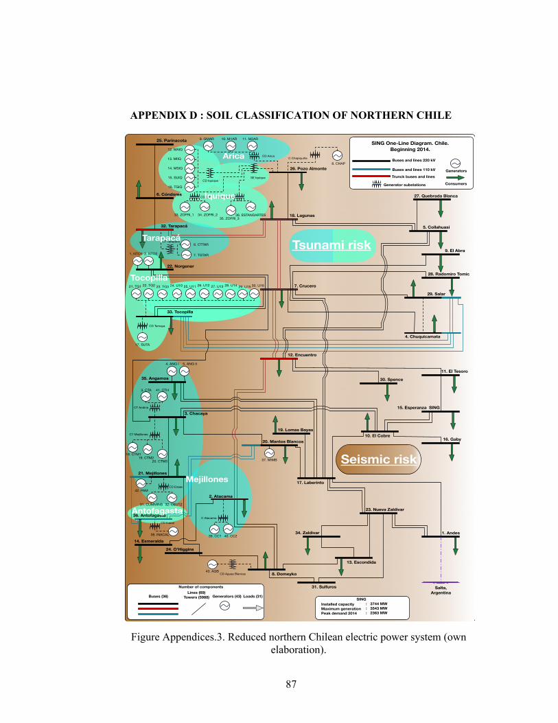
87
APPENDIX D : SOIL CLASSIFICATION OF NORTHERN CHILE
Figure Appendices.3. Reduced northern Chilean electric power system (own elaboration).
CT Andina
CT Tarapacá
C ChapiquiñaCD Arica
CD IquiqueSE Iquique
CD Tamaya
CT Mejillones
CD Enaex
CD Zofri Estandartes
CD InacalC Atacama
CD Aguas Blancas
Salta,Argentina
36. Antofagasta
35. Angamos
34. Zaldivar
33. Tocopilla
32. Tarapacá
31. Sulfuros
30. Spence
29. Salar
28. Radomiro Tomic
27. Quebrada Blanca
26. Pozo Almonte
25. Parinacota
24. O’Higgins
23. Nueva Zaldivar
22. Norgener
21. Mejillones
20. Mantos Blancos
19. Lomas Bayas
18. Lagunas
17. Laberinto
16. Gaby
15. Esperanza SING
14. Esmeralda
13. Escondida
12. Encuentro
11. El Tesoro
10. El Cobre
9. El Abra
8. Domeyko
7. Crucero
6. Cóndores
5. Collahuasi
4. Chuquicamata
3. Chacaya
2. Atacama
1. Andes
Number of components
Buses (36) Generators (43) Loads (31)Lines (69)
Towers (5988)
SING One-Line Diagram. Chile. Beginning 2014.
Trunck buses and lines
Buses and lines 220 kV
Generators
Consumers
Buses and lines 110 kV
Generator substations
SINGInstalled capacityMaximum generationPeak demand 2014
: 3744 MW: 3543 MW : 2363 MW
43. AGB
42. PAM
41. CTH
40. CC239. CC138. INACAL
37. MIMB
36. ESTANDARTES35. ZOFRI_3
34. ZOFRI_233. ZOFRI_1
32. DEUTZ31. CUMMINS
30. U1629. U1528. U1427. U1326. U1225. U1124. U1023. TG322. TG221. TG1
20. CTM319. CTM2
18. CTM1
17. SUTA
16. TGIQ
15. SUIQ
14. MSIQ
13. MIIQ
12. MAIQ
11. M2AR10. M1AR9. GMAR
8. CHAP
7. TGTAR
6. CTTAR
5. ANG II4. ANG I
3. CTA
2. NTO21. NTO1
Tarapacá
Iquique
Arica
Tocopilla
Mejillones
Antofagasta
Tsunami risk
Seismic risk

88
APPENDIX E : NORTHERN CHILEAN HAZARD MAP
Figure Appendices.4. VS30 in northern Chile (USGS).

89
APPENDIX F : INTERNATIONAL LITERATURE OF SEISMIC
FRAGILITY CURVES FOR ELECTRICAL COMPONENTS
Fragility curves found were presented in WCEE, the World Conferences on Earthquake Engineering, and in the Syner-G project. The detailed publications reviewed are presented in Table Appendices.1.
Table Appendices.1. Seismic fragility curves for electrical components presented in WCEE and Syner-G project.
Reference Elements studied Earthquake intensity measure
Damage states used
Sadeghi, et al. 2012. Tubular steel towers.
Peak ground acceleration.
Failure.
XIE, et al. 2012. Lattice steel towers. Peak ground acceleration.
Minor, Major and Collapse.
Anagnos. 1999. 6 microcomponents. Peak ground acceleration.
Failure modes depending on the component.
Anagnos and Ostrom. 2000
500 kV circuit breaker and 230 kV horizontal disconnect switch.
Peak ground acceleration.
Failure modes depending on the component.
Ang, Pires and Villaverde. 1996.
6 microcomponents and 500 kV-230 kV substations.
Peak ground acceleration.
Failure.
Bettinali, et al. 2004.
11 microcomponents.
Peak ground acceleration.
Failure.
Dueñas-Osorio, Craif and Goodno. 2007.
Electric power grid. Peak ground acceleration.
Failure based on substation functionality (20, 50 and 80%).
Giovinazzi and King. 2009.
Medium voltage substation.
Peak ground acceleration.
Minor, Moderate, Extensive and Complete.
Hwang and Huo. 1998.
9 microcomponents, pothead structure and 115/12 kV transformer.
Peak ground acceleration.
Failure.
Hwang and Chou. 1998.
6 microcomponents and substation.
Peak ground acceleration.
Failure.

90
Liu, et al. 2003. 500 kV – 230 kV three-phase transformers.
Peak ground acceleration.
Failure.
Rasulo, et al. 2004. 11 microcomponents and substation.
Peak ground acceleration.
Failure.
Straub and Kiureghian. 2008.
1-phase 230 kV transformer, 230 kV live tank circuit breaker and systems of these components
Peak ground acceleration.
Failure.
Vanzi. 1996. 11 microcomponents and 4 macrocomponents
Peak ground acceleration.
Failure.
Vanzi. 2000. Distribution substation
Peak ground acceleration.
Failure.
Vanzi, et al. 2004. 420 kV circuit breaker
Spectral acceleration.
Failure.
Shinozuka, et al. 2007.
Transformer, circuit breaker, disconnect switch and bus
Peak ground acceleration.
Failure.
Hazus, FEMA. 2003.
Substation, distribution circuits and power plants.
Peak ground acceleration.
Minor, Moderate, Extensive and Complete.

91
APPENDIX G : SING’S RECUPERATION ZONES
Figure Appendices.5. Reduced northern Chilean electric power system (own elaboration).
Zona Norte
Zona Centro
Zona Cordillera
Zona Sur
Área Arica
Área Iquique
Área Tarapacá
Área Capricornio
Área O’Higgins
CT Andina
CT Tarapacá
C ChapiquiñaCD Arica
CD IquiqueSE Iquique
CD Tamaya
CT Mejillones
CD Enaex
CD Zofri Estandartes
CD InacalC Atacama
CD Aguas Blancas
Salta,Argentina
36. Antofagasta
35. Angamos
34. Zaldivar
33. Tocopilla
32. Tarapacá
31. Sulfuros
30. Spence
29. Salar
28. Radomiro Tomic
27. Quebrada Blanca
26. Pozo Almonte
25. Parinacota
24. O’Higgins
23. Nueva Zaldivar
22. Norgener
21. Mejillones
20. Mantos Blancos
19. Lomas Bayas
18. Lagunas
17. Laberinto
16. Gaby
15. Esperanza SING
14. Esmeralda
13. Escondida
12. Encuentro
11. El Tesoro
10. El Cobre
9. El Abra
8. Domeyko
7. Crucero
6. Cóndores
5. Collahuasi
4. Chuquicamata
3. Chacaya
2. Atacama
1. Andes
43. AGB
42. PAM
41. CTH
40. CC239. CC138. INACAL
37. MIMB
36. ESTANDARTES35. ZOFRI_3
34. ZOFRI_233. ZOFRI_1
32. DEUTZ31. CUMMINS
30. U1629. U1528. U1427. U1326. U1225. U1124. U1023. TG322. TG221. TG1
20. CTM319. CTM2
18. CTM1
17. SUTA
16. TGIQ
15. SUIQ
14. MSIQ
13. MIIQ
12. MAIQ
11. M2AR10. M1AR9. GMAR
8. CHAP
7. TGTAR
6. CTTAR
5. ANG II4. ANG I
3. CTA
2. NTO21. NTO1
SING
SING One-Line Diagram. Chile. Beginning 2014.
Trunck buses and lines
Buses and lines 220 kV
Generators
Consumers
Buses and lines 110 kV
Generator substations
Number of components
Buses (36) Generators (43) Loads (31)Lines (69)
Towers (5988)
Generator with autonomous start up

92
APPENDIX H : LIST OF PUBLICATIONS AND PRESENTATIONS
SUBMITTED JOURNAL PAPERS
S. Espinoza, H. Rudnick, M. Panteli and P. Mancarella, “Multi-phase assessment and
adaptation of power systems resilience to natural hazards," Under revision, Electric
Power Systems Research, Elsevier. August 2015.
TO-BE-SUBMITTED JOURNAL PAPERS
S. Espinoza, H. Rudnick, A. Poulos, J. Gonzáles, M. Panteli, P. Mancarella, R. Moreno
and J.C. de la Llera, “Multi-phase assessment and adaptation of power systems
resilience to earthquakes and tsunamis," To be submitted, IEEE Transactions on Power
Systems.
PRESENTATIONS
S. Espinoza, H. Rudnick, M. Panteli and P. Mancarella, “Resilience assessment of
electric power systems after the impact on natural disasters," poster presented in PGR
Poster Conference, Manchester, UK, May 2015.