multi-dimensional classification with probabilistic...
TRANSCRIPT
Comprehensive Exam
Multi-dimensional Classificationwith Probabilistic Graphical Models
and Ensemble Techniques
Charmgil Hong
Committee: Dr. Milos Hauskrecht Dr. Jingtao Wang Dr. Rebecca Hwa
Agenda
• Motivation + Problem Definition
• Multi-dimensional Classification
• Probabilistic Graphical Models
• Ensemble Techniques
2
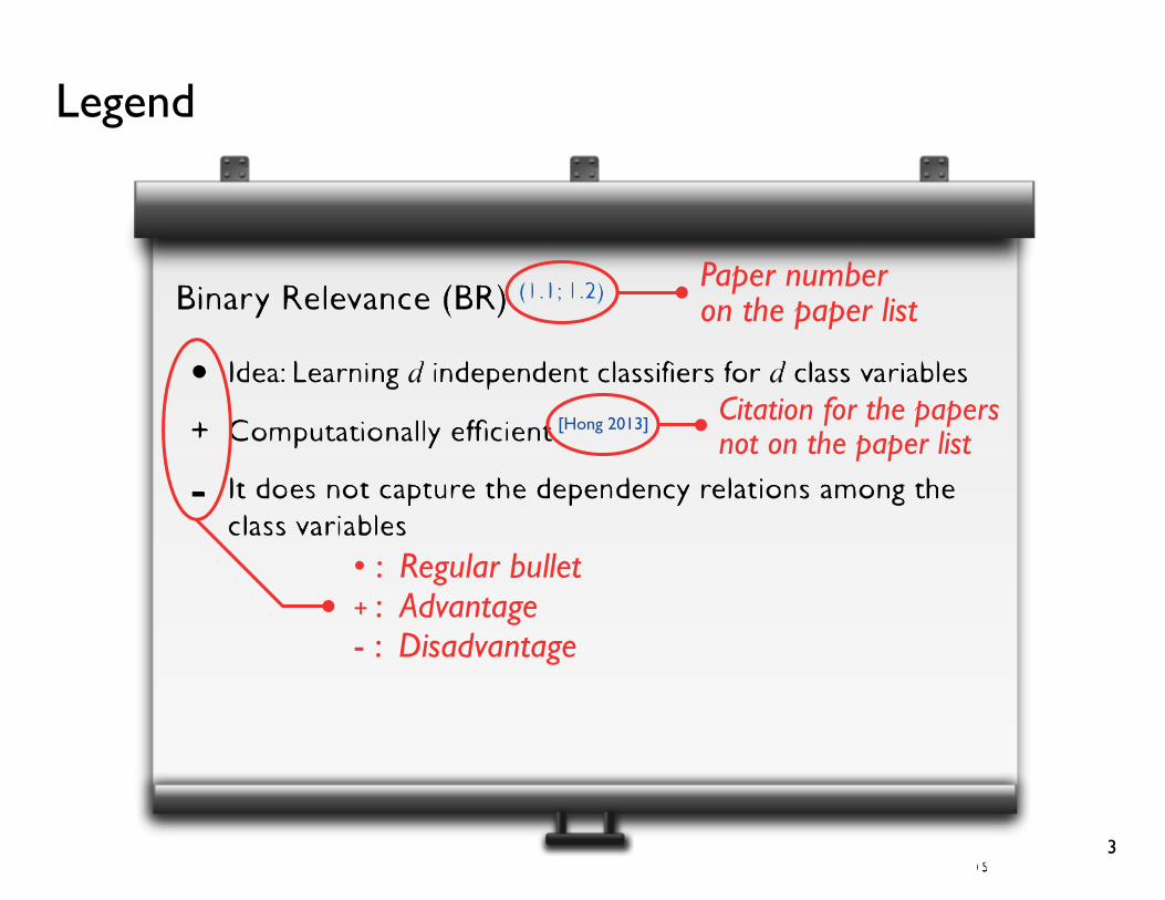
Legend
3
Paper numberon the paper list
• : Regular bullet+ : Advantage- : Disadvantage
[Hong 2013] Citation for the papersnot on the paper list

Notation
• X ∈ Rm : feature vector variable (input)
• Y ∈ Rd : label vector variable (output)
• x = {x1, ..., xm}: feature vector instance
• y = {y1, ..., yd}: label vector instance
• In a shorthand, P(Y=y|X=x) = P(y|x)
• Dtrain : training dataset; Dtest : test dataset
• i = 1, ..., d : class variable (Y) index
• j = 1, ..., m : feature (X) index
• n = 1, ..., N : instance index
• k = 1, ..., K : component index (in ensembles or mixtures)
4

Motivation
• Traditional classification
• Each data instance is associated with a single class variable
5

Motivation
• An issue with traditional classification
• In many real-world applications, each data instance can be associated with multiple class variables
• Examples
• A news article may cover multiple topics, such as politics and economy
• An image may include multiple objects as building, road, and car
• A gene may be associated with several biological functions
6

Problem Definition
• Multi-dimensional classification (MDC)
• Each data instance is associated with multiple class variables
• Objective: assign each instance the most probable assignment of the class variables
7
Class 1 ∈ { R, G, B } Class 2 ∈ { , }
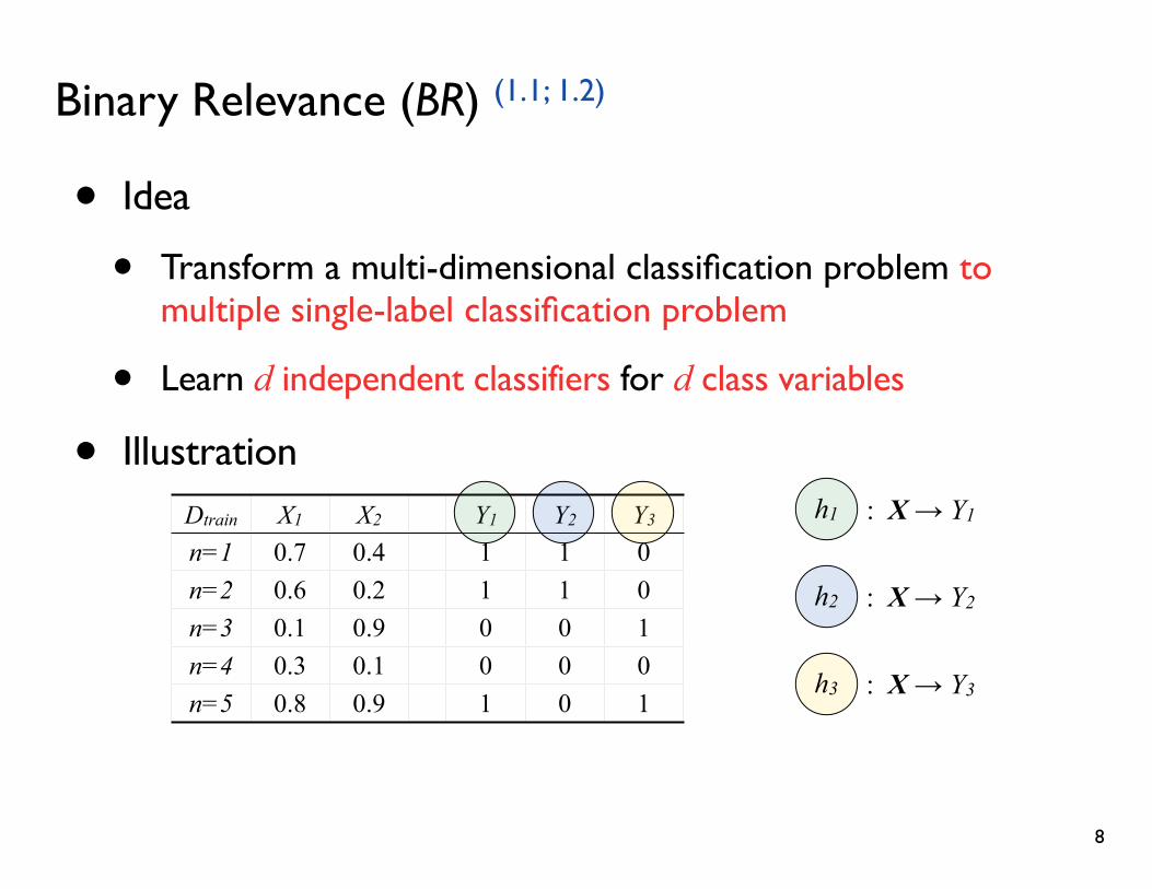
Binary Relevance (BR) (1.1; 1.2)
• Idea
• Transform a multi-dimensional classification problem to multiple single-label classification problem
• Learn d independent classifiers for d class variables
• Illustration
8
Dtrain X1 X2 Y1 Y2 Y3
n=1 0.7 0.4 1 1 0n=2 0.6 0.2 1 1 0n=3 0.1 0.9 0 0 1n=4 0.3 0.1 0 0 0n=5 0.8 0.9 1 0 1
h1 : X → Y1
h2 : X → Y2
h3 : X → Y3

Binary Relevance (BR) (1.1; 1.2)
• Discuss
+ Computationally efficient
- Does not capture the dependence relations among the class variables
- The objective is not suitable for MDC
- Does not find the most probable assignment
- Instead, it maximizes the marginal distribution of each class variable
9

Marginal vs. Joint: a motivating example
• Find the most probable assignment (MAP; maximum a posteriori) of Y
10
P(Y1,Y2|X=x) Y1 = 0 Y1 = 1 P(Y2|X=x)Y2 = 0 0.2 0.45Y2 = 1 0.35 0
P(Y1|X=x)
➡ Prediction on the marginals: Y1 = 0, Y2 = 0➡ Prediction on the joint (MAP): Y1 = 1, Y2 = 0
• We want to maximize the joint distribution of Y given observation X = x; i.e.,
P(Y1,Y2|X=x) Y1 = 0 Y1 = 1 P(Y2|X=x)Y2 = 0 0.2 0.45 0.65Y2 = 1 0.35 0 0.35
P(Y1|X=x) 0.55 0.45
P(Y1,Y2|X=x) Y1 = 0 Y1 = 1 P(Y2|X=x)Y2 = 0 0.2 0.45 0.65Y2 = 1 0.35 0 0.35
P(Y1|X=x) 0.55 0.45

Challenge
• The number of possible label assignments is exponential in the number of labels
• Finding the the most probable assignment out of O(|ΩY|d) possible label combinations, where |ΩY| is the number of possible values for a label
11

Agenda
✓ Motivation + Problem Definition
• Multi-dimensional Classification
• Probabilistic Graphical Models
• Ensemble Techniques
12
• Multi-dimensional Classification
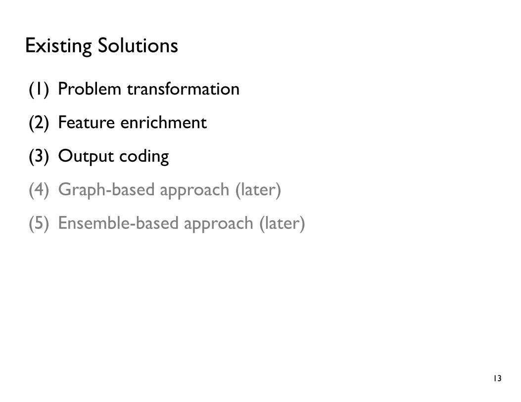
Existing Solutions
(1) Problem transformation
(2) Feature enrichment
(3) Output coding
(4) Graph-based approach (later)
(5) Ensemble-based approach (later)
13
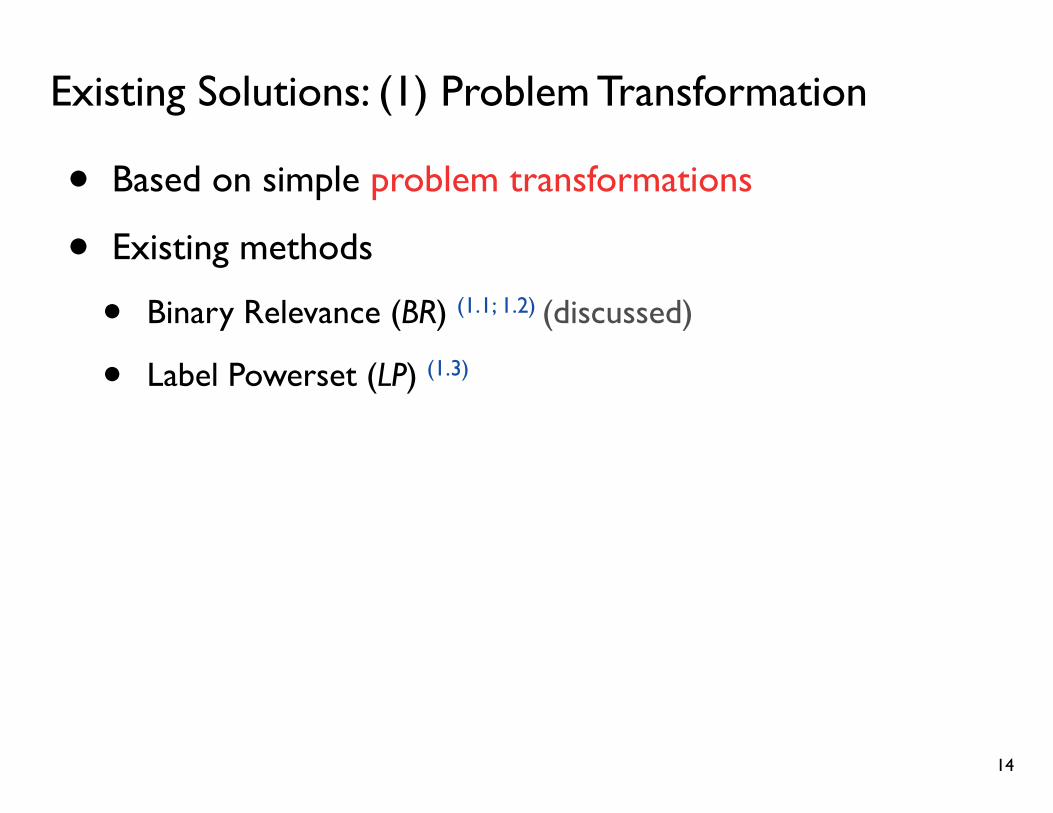
Existing Solutions: (1) Problem Transformation
• Based on simple problem transformations
• Existing methods
• Binary Relevance (BR) (1.1; 1.2) (discussed)
• Label Powerset (LP) (1.3)
14

Label Powerset (LP) (1.3)
• Idea
i) Transform each label combination to a class variableii) Learn a multi-class classifier with the new class variable
• Illustration
15
Dtrain X1 X2 Y1 Y2 Y3
n=1 0.7 0.4 1 1 0n=2 0.6 0.2 1 1 0n=3 0.1 0.9 0 0 1n=4 0.3 0.1 0 0 0n=5 0.8 0.9 1 0 1
YLP
11234
hLP : X → YLP

Label Powerset (LP) (1.3)
• Discuss
+ Learns the full joint of the class variables
+ Each of the new class values maps to a label combination
- The number of choices in the new class can be exponential (|YLP| = O(|Ω|d))
- Learning a multi-class classifier on exponential choices is expensive
- The resulting class would be sparse and imbalanced
16

Further Discuss: (1) Problem Transformation
• BR maximizes the marginals on each class label;while LP directly models the joint of all class labels
- Neither considers the relationships among class labels
17
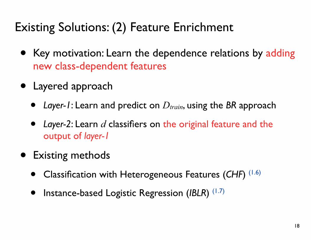
Existing Solutions: (2) Feature Enrichment
• Key motivation: Learn the dependence relations by adding new class-dependent features
• Layered approach
• Layer-1: Learn and predict on Dtrain, using the BR approach
• Layer-2: Learn d classifiers on the original feature and the output of layer-1
• Existing methods
• Classification with Heterogeneous Features (CHF) (1.6)
• Instance-based Logistic Regression (IBLR) (1.7)
18
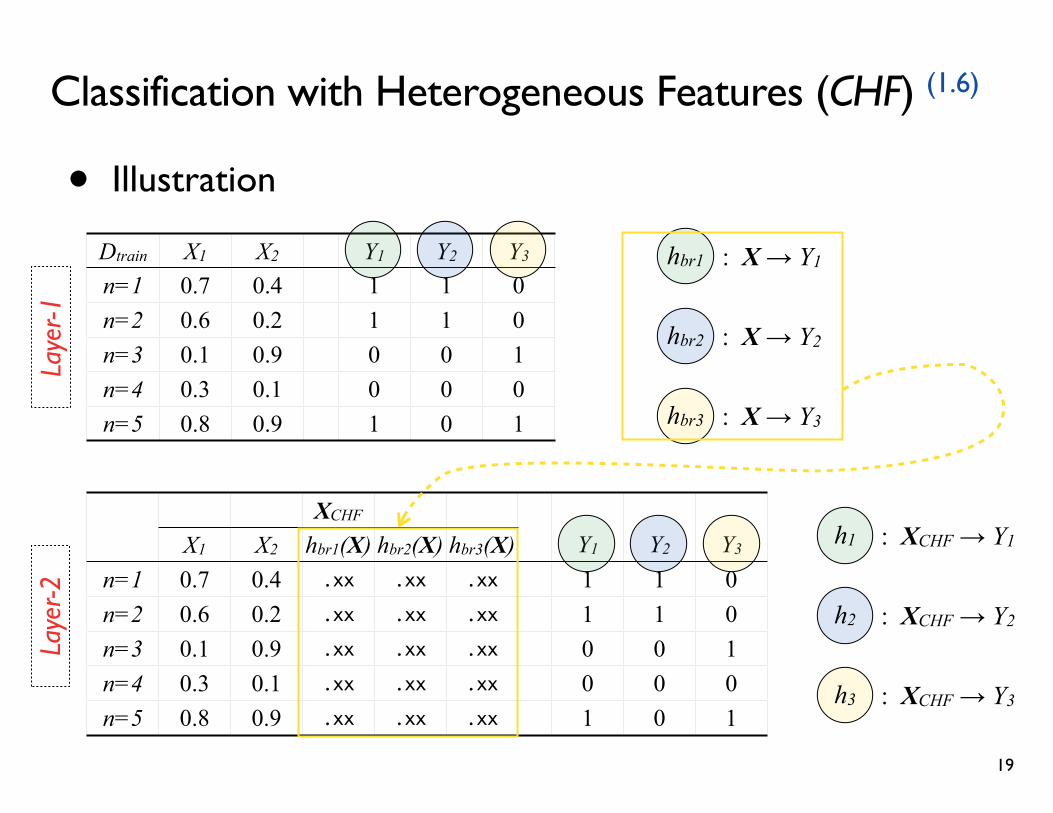
Classification with Heterogeneous Features (CHF) (1.6)
• Illustration
19
Dtrain X1 X2 Y1 Y2 Y3
n=1 0.7 0.4 1 1 0n=2 0.6 0.2 1 1 0n=3 0.1 0.9 0 0 1n=4 0.3 0.1 0 0 0n=5 0.8 0.9 1 0 1
hbr1 : X → Y1
hbr2 : X → Y2
hbr3 : X → Y3
XCHF
X1 X2 hbr1(X) hbr2(X) hbr3(X) Y1 Y2 Y3
n=1 0.7 0.4 .xx .xx .xx 1 1 0n=2 0.6 0.2 .xx .xx .xx 1 1 0n=3 0.1 0.9 .xx .xx .xx 0 0 1n=4 0.3 0.1 .xx .xx .xx 0 0 0n=5 0.8 0.9 .xx .xx .xx 1 0 1
h1 : XCHF → Y1
h2 : XCHF → Y2
h3 : XCHF → Y3
Laye
r-1La
yer-2
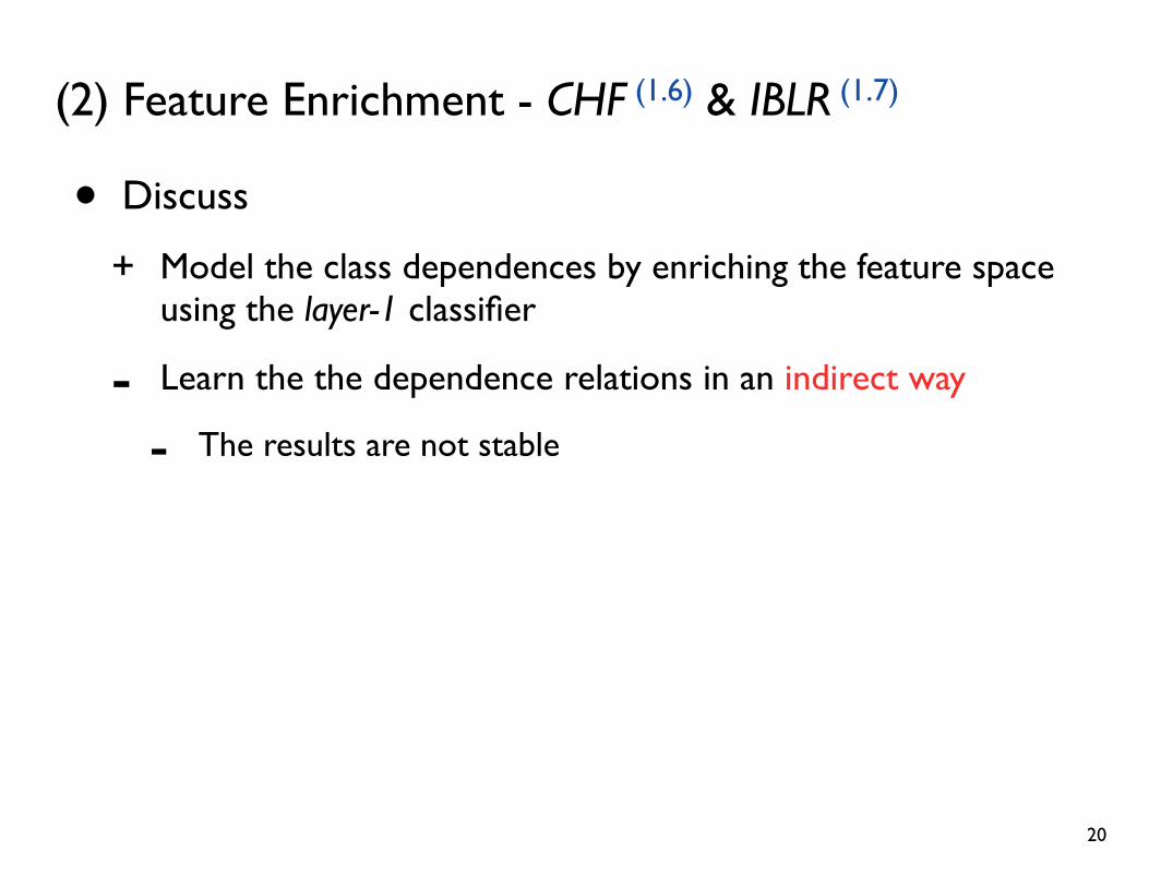
(2) Feature Enrichment - CHF (1.6) & IBLR (1.7)
• Discuss
+ Model the class dependences by enriching the feature space using the layer-1 classifier
- Learn the the dependence relations in an indirect way
- The results are not stable
20

Existing Solutions: (3) Output Coding
• Key motivation
• Motivated by the error-correcting output coding (ECOC) scheme [Dietterich 1995; Bose & Ray-Chaudhuri 1960] in communication
• Solve the MDC problems using lower dimensional codewords
• Output coding scheme usually contains three parts:
• Encoding:
• Prediction:
• Decoding:
21
Convert output vectors Y into codewords Z
Perform regression from X to Z; say R
Recover the class labels Y from R
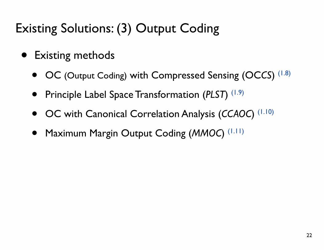
Existing Solutions: (3) Output Coding
• Existing methods
• OC (Output Coding) with Compressed Sensing (OCCS) (1.8)
• Principle Label Space Transformation (PLST) (1.9)
• OC with Canonical Correlation Analysis (CCAOC) (1.10)
• Maximum Margin Output Coding (MMOC) (1.11)
22

Existing Solutions: (3) Output Coding
• Existing methods
23
Method Key difference
OCCS (1.8) Uses compressed sensing [Donoho 2006] for encoding and decoding
PLST (1.9) Uses singular vector decomposition (SVD) [Johnson & Wichern 2002] for encoding and decoding
CCAOC (1.10) Uses canonical correlation analysis (CCA) [Johnson & Wichern 2002] for encoding and mean-field approximation (2.1) for decoding
MMOC (1.11) Uses SVD for encoding and maximum margin formulation for decoding

Existing Solutions: (3) Output Coding
• Discuss
+ Show excellent prediction performances
- Only able to predict the single best output for a given input
- Cannot estimate probabilities for different input-output pairs
- Not scalable
- Encoding and decoding steps rely on matrix decomposition, whose complexities are sensitive to d and N
- Work with binary labels only
24

Section Summary: Multi-dimensional Classification
• MDC problems formulate the situations where an instance can be associated with more than one class label
• Main issue is that the size of the label space is exponential
• To tackle the problems, a range of approaches has been proposed
• Approaches fall in problem transformation, feature enrichment, and output coding have been introduces
• Graph-based and ensemble-based methods will be discussed later
25
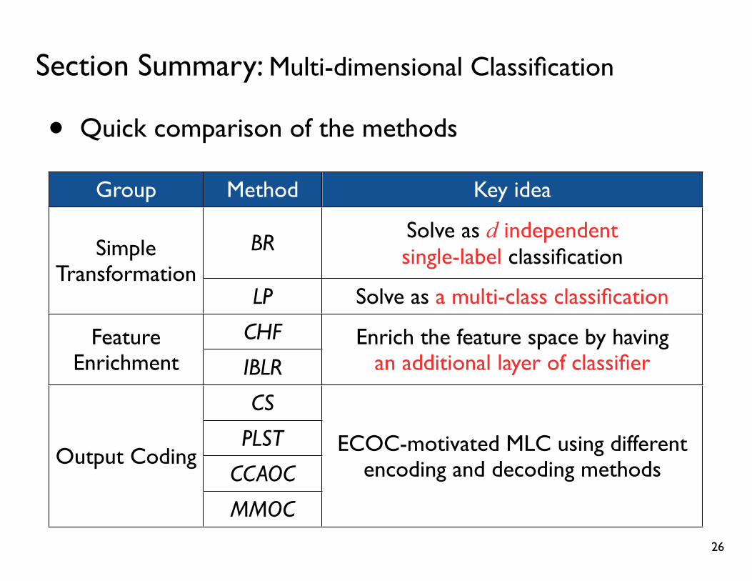
Section Summary: Multi-dimensional Classification
• Quick comparison of the methods
26
Group Method Key idea
Simple Transformation
BR Solve as d independent single-label classificationSimple
TransformationLP Solve as a multi-class classification
Feature Enrichment
CHF Enrich the feature space by having an additional layer of classifier
Feature Enrichment IBLR
Enrich the feature space by having an additional layer of classifier
Output Coding
CS
ECOC-motivated MLC using different encoding and decoding methodsOutput Coding
PLST ECOC-motivated MLC using different encoding and decoding methodsOutput Coding
CCAOCECOC-motivated MLC using different
encoding and decoding methodsOutput Coding
MMOC
ECOC-motivated MLC using different encoding and decoding methods
Agenda
✓ Motivation + Problem Definition
✓ Multi-dimensional Classification
• Probabilistic Graphical Models
• Ensemble Techniques
27
• Probabilistic Graphical Models (PGM)
Section Agenda
• Overview
• Motivation
• Definition
• Fundamental
• Task
• Structure Learning
• Parameter Learning
• Inference
• Case Study: PGM on Multi-dimensional Classification28
• Probabilistic Graphical Models (PGM)

Motivation: PGM
• In many applications, we need to use a large number of random variables, which may induce a complex model
• PGM tackles this issue by exploiting the independence relations among variables
29

Definition: PGM
• Formal Definition (2.1)
• PGM refers to a family of distributions on a set of random variables that are compatible with all the probabilistic independence propositions encoded in a graph
• Informal Definition
• PGM = Multivariate statistics + Graphical structure
• A smart way to formulate exponentially large probability distribution without paying an exponential cost
30

Fundamental: Representation
• Two types
• Directed graphical models (DGMs)
• Also known as Bayesian networks (BNs)
• Undirected graphical models (UGMs)
• Also known as Markov networks (MNs)
31
X1
X2
X1
X2
Directed(BN)
Undirected(MN)
node: variable
edge:causal relation
edge:correlation

Fundamental: How PGM Reduces the Complexity?
• Key idea: Exploit the conditional independence (CI) relations among variables!!
• Conditional independence (CI): Random variables A, B are conditionally independent given C, if P(A,B|C) = P(A|C)P(B|C)
• DGM and UGM offer a set of graphical notations for CI
32
A ⊥ B | CA ⊥ B | C A ⊥ B | C
CI representations in DGMCI representations in DGMCI representations in DGM
⧸
A B
CA BC
A B
C

Fundamental: How PGM Reduces the Complexity?
• Key idea: Exploit the conditional independence (CI) relations among variables!!
• Conditional independence (CI): Random variables A, B are conditionally independent given C, if P(A,B|C) = P(A|C)P(B|C)
• DGM and UGM offer a set of graphical notations for CI
33
A ⊥ B | C
CI representation in UGM
A B
C

Fundamental: How CI Reduces the Complexity?
• CI makes the models decomposable!
• Example: Recall the famous Earthquake-Burglary example (2.1)
• #Parameters for full joint = 31
• #Parameters for BN = 10
34
BurglaryEarthquake
Alarm
MarryCallsJohnCalls
⬅︎ P(E,B,A,J,M)
⬅︎ P(J|A)P(M|A)P(A|E,B)P(E)P(B)
Fundamental: How to Apply PGM to a Problem?
• We need to
• Learn the model structure - in/dependent relations among variables - from data
• Learn the parameters of the model from data
• Use the model to make inferences
35

Task
(1) Structure Learning
(2) Parameter Learning
(3) Inference
36
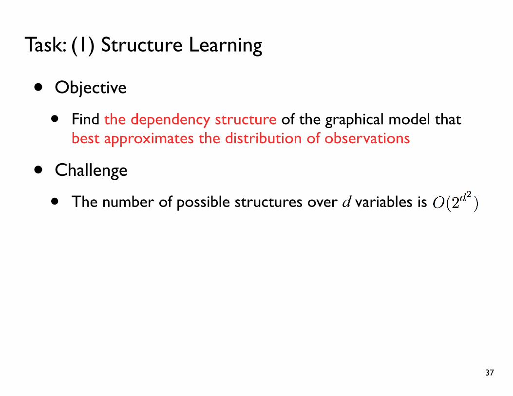
Task: (1) Structure Learning
• Objective
• Find the dependency structure of the graphical model that best approximates the distribution of observations
• Challenge
• The number of possible structures over d variables is O
37

Task: (1) Structure Learning
• Approaches
38
TypeType Description / Method
Score-based
Likelihood score Search for the structure that maximizesmutual information or likelihood of data
Score-based
Bayesian score Find the model fitness - model complexitytrade off
Constraint-basedConstraint-based Build a structure by applyinga set of rules (constraints) to data
Bayesian model averagingBayesian model averaging Keep all possible structures and their probabilities
Description / Method
Chow-Liu algorithm [Chow-Liu 1968],K2 algorithm (2.7), CTBN (2.17)
Akaike Information Criterion (AIC) (2.1),Bayesian Information Criterion (BIC) (2.1)
PC algorithm [Spirtes & Glymour 1991]
Bayesian model averaging [Hoeting et al. 1999]
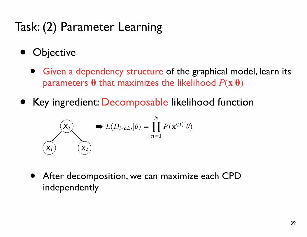
Task: (2) Parameter Learning
• Objective
• Given a dependency structure of the graphical model, learn its parameters θ that maximizes the likelihood P(x|θ)
• Key ingredient: Decomposable likelihood function
• After decomposition, we can maximize each CPD independently
39
X1 X2
X3 ➡ ︎

Task: (3) Inference
• Objective
• Answer queries about the distribution
• Types of queries
• Likelihood query: P(Xobs = xobs)
• Conditional probability query: P(Xquery = xquery|Xobs = xobs)
• MAP prediction: argmax P(xquery|xobs)
40
xquery

Task: (3) Inference
• Challenge
• Inference is essentially a marginalization step on the joint distribution which is exponential
• Solutions
41
Approach Idea / Method
Approximate the target
distribution
For general graphs, exact inference is infeasible.Approximate the distribution
using surrogates, sampling, relaxation.
Restrict the structure
For certain structures, such as chain or tree,we can perform exact inference in polynomial time
Mean field approximation (2.8), Sampling methods (2.1),Loopy belief propagation (2.12)
Variable elimination (2.1), Belief propagation (2.1; 2.17)

Section Agenda
• Probabilistic Graphical Models
✓ Motivation
✓ Definition
✓ Fundamentals
✓ Task
✓ Structure Learning
✓ Parameter Learning
✓ Inference
• Case Study: PGM on Multi-dimensional Classification
42

Case Study: PGM on Multi-dimensional Classification
• PGM has been an excellent representation / formulation tool for the MDC problems
• Existing methods
• Bayesian networks (directed)
• Classifier Chains (CC) (2.13)
• Multi-dimensional Bayesian Classifiers (MBC) (2.9; 2.10)
• Conditional Tree-structured Bayesian Networks (CTBN) (2.17)
• Markov networks (undirected)
• Multi-label Conditional Random Field (ML-CRF) (2.11)
• Composite Marginal Models (CMM) (2.12)
43

Classifier Chains (CC) (2.13)
• Key idea
• Build a chain of class variables, where all preceding classes are conditioning the following class variables in the chain
• Representation
44
all preceding labels
Y1 Y2 Y3 Yd...
X

Classifier Chains (CC) (2.13)
• Tasks on CC
• No structure learning (random chain order)
• Parameter learning is performed on the decomposed CPDs:
argmax P(Yi|X, π(Yi), θ) : on each CPD
• Inferences is performed by maximizing each CPDs:
argmax P(Yi|X, π(Yi), θ) : on each CPD
45
Y1 Y2 Y3 Yd...
θ
Yi

Conditional Tree-structured Bayesian Networks (CTBN) (2.17)
• Key idea
• Learn a tree-structured Bayesian network of the class labels
• Example CTBN
46
X
Y1 Y2 Y3 Y4
at most one parent label

Conditional Tree-structured Bayesian Networks (CTBN) (2.17)
• Tasks on CTBN
• Score-based structure learning
1. Define a complete weighted directed graph, whose edge weights is equal to conditional log-likelihood
2. Find the maximum branching tree from the graph
• Maximum branching tree = maximum weighted directed spanning tree
47
X
Y1 Y2 Y3 Y4

CTBN: Structure Learning (2.17)
1. Define a complete weighted directed graph, whose edges are weighted by conditional log-likelihood:
48
Y1 Y2
Y3Y4
W1→2
W2→1
W4→3
W3→4W
4→1
W1→
4
W3→
2
W2→
3W1→
3
W3→
1
W4→2
W2→4
W𝜙→1 W𝜙→2
W𝜙→3W𝜙→4

CTBN: Structure Learning (2.17)
2. Find the tree that maximizes the sum of the edge weights by solving the maximum branching tree problem
49
Y1 Y2
Y3Y4
W1→2
W2→1
W4→3
W3→4W
4→1
W1→
4
W3→
2
W2→
3W1→
3
W3→
1
W4→2
W2→4
W𝜙→1 W𝜙→2
W𝜙→3W𝜙→4

Conditional Tree-structured Bayesian Networks (CTBN) (2.17)
• Tasks on CTBN
• Score-based structure learning
• Parameter learning is performed on the decomposed CPDs
• Exact MAP prediction is performed by belief propagation
50
X
Y1 Y2 Y3 Y4
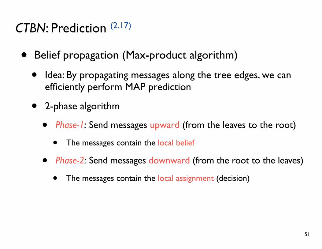
CTBN: Prediction (2.17)
• Belief propagation (Max-product algorithm)
• Idea: By propagating messages along the tree edges, we can efficiently perform MAP prediction
• 2-phase algorithm
• Phase-1: Send messages upward (from the leaves to the root)
• The messages contain the local belief
• Phase-2: Send messages downward (from the root to the leaves)
• The messages contain the local assignment (decision)
51
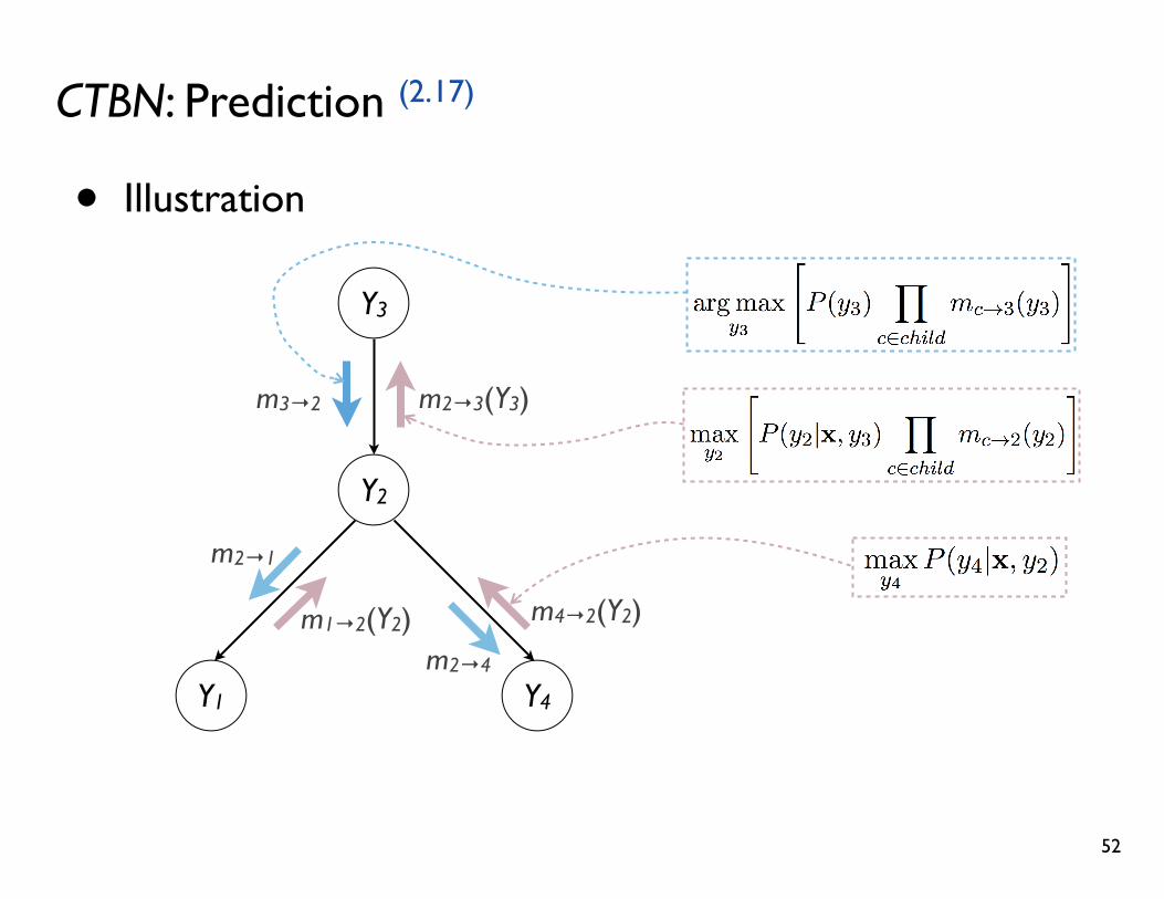
CTBN: Prediction (2.17)
• Illustration
52
Y1
Y2
Y3
Y4
m4→2(Y2)m1→2(Y2)
m2→3(Y3)m3→2
m2→1
m2→4

Further Discuss: CC (2.13) vs. CTBN (2.17)
53
CC CTBN
X
Y1 Y2 Y3 Y4
Y1 Y2 Y3 Yd...
at most one parent labelall preceding labels
• No structure learning (label ordering is given at random)
• Tree structure is learned using a score-based algorithm
• Performs exact MAP prediction• Maximizes the marginals along the chain (suboptimal solution)
• Errors in prediction propagate to the following label prediction
• The tree-structure assumption may restrict its modeling ability
Section Summary
• PGM offers a way to formulate a exponentially large probability distribution without an exponential cost
• PGM provides various methods to perform structure learning, parameter learning, and inference
• PGM can be a good formulation tool for the MDC problems
• CC and CTBN have been discussed
54

Agenda
✓ Motivation + Problem Definition
✓ Multi-dimensional Classification
✓ Probabilistic Graphical Models
• Ensemble Techniques
55
• Ensemble Techniques
Section Agenda
• Overview
• Definition
• Motivation
• Key Criteria
• Popular Techniques
• Ensemble of Multi-dimensional Classifiers
56
• Ensemble Techniques

Definition: Ensemble Techniques
• Techniques of training multiple classifiers and combining their predictions to produce a single classifier
• Objective: Make a combination of simpler classifiers to improve predictions
57
Motivation (3.1; 3.3)
(1) Statistical reason
(2) Computational reason
(3) Representational reason
58
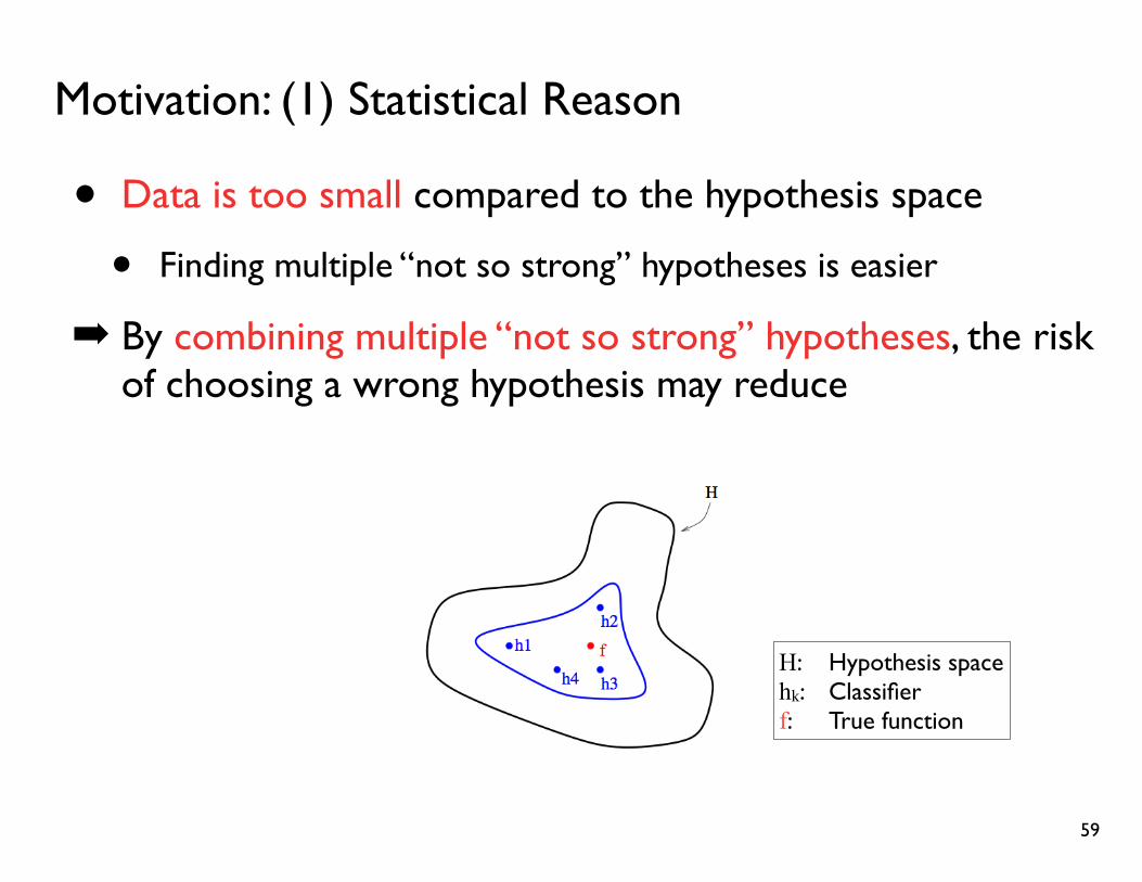
Motivation: (1) Statistical Reason
• Data is too small compared to the hypothesis space
• Finding multiple “not so strong” hypotheses is easier
➡ By combining multiple “not so strong” hypotheses, the risk of choosing a wrong hypothesis may reduce
59
H: Hypothesis spacehk: Classifierf: True function

Motivation: (2) Computational Reason
• Data is too much to generalize
• Many learning algorithms perform local search; may get stuck in local optima
➡ By running the local search from many different starting points, a better approximation would be obtained
60
H: Hypothesis spacehk: Classifierf: True function

Motivation: (3) Representational Reason
• Certain problems are just too difficult to learn
• The true function cannot be represented by any hypothesis in the hypotheses space
➡ By doing ensemble, the space of representable functions may expand
61
H: Hypothesis spacehk: Classifierf: True function
Key Criteria (3.3)
• Base classifiers should be accurate and diverse
• Quote: “highly correct classifiers that disagree as much as possible” [Krogh & Vedelsby 1995]
• Strategy to combine predictions should be effective
62

Key Criteria (3.3)
• Base classifiers should be accurate and diverse
• Quote: “highly correct classifiers that disagree as much as possible” [Krogh & Vedelsby 1995]
• Strategy to combine predictions should be effective
63
Section Agenda
• Ensemble Techniques
✓ Overview
✓ Definition
✓ Motivation
✓ Key Criteria
• Popular Techniques
• Ensembles of Multi-dimensional Classifiers
64
Popular Techniques
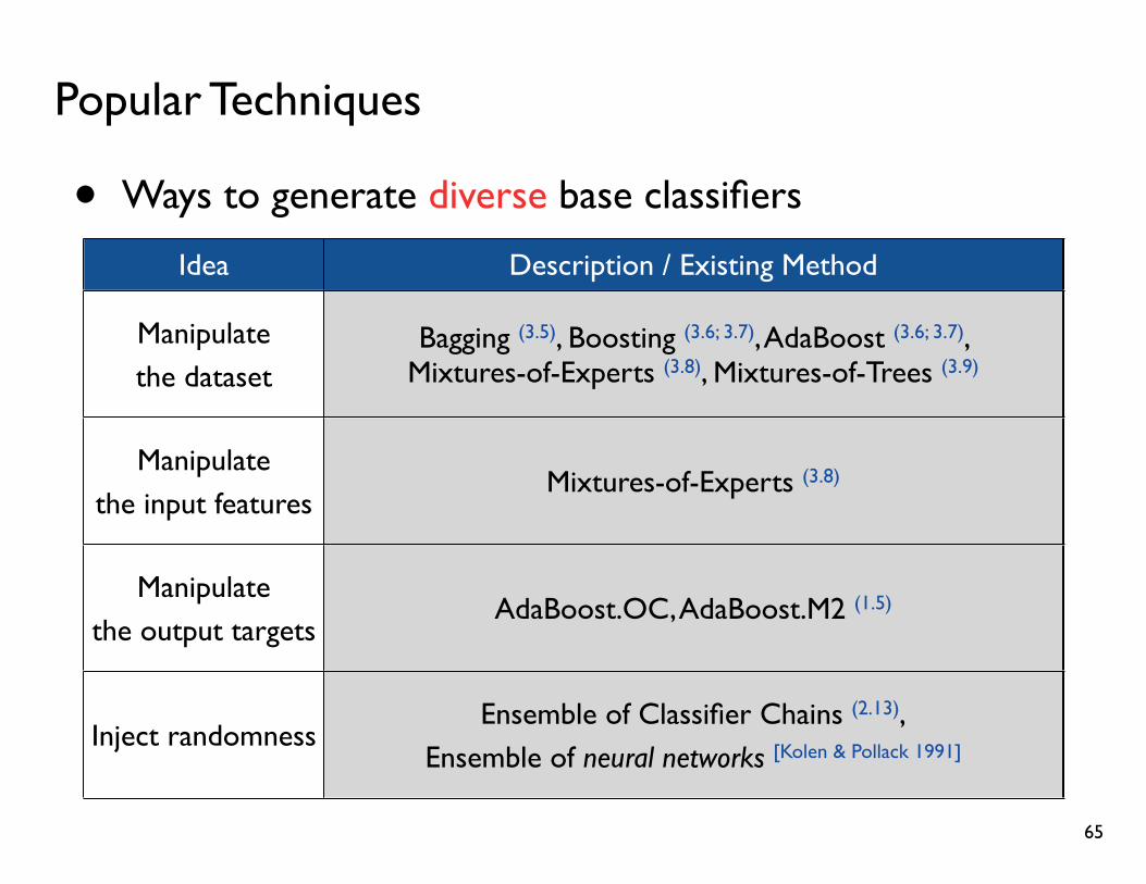
• Ways to generate diverse base classifiers
65
Idea Description / Method
Manipulate the dataset
Train classifiers on different datasets, created by bootstrapping or weighted resampling
Manipulate the input features
Train classifiers on different input feature sets
Manipulate the output targets
Convert output to another format;e.g., a multi-class label to multiple binary labels
Inject randomnessInject randomness to the model;
e.g., training with different initial parameters
Description / Existing Method
Bagging (3.5), Boosting (3.6; 3.7), AdaBoost (3.6; 3.7), Mixtures-of-Experts (3.8), Mixtures-of-Trees (3.9)
Mixtures-of-Experts (3.8)
AdaBoost.OC, AdaBoost.M2 (1.5)
Ensemble of Classifier Chains (2.13),Ensemble of neural networks [Kolen & Pollack 1991]

Popular Techniques
• Ways to combine multiple predictions
66
Idea Description / Existing Method
Averaging(majority vote)
Simple averaging on multiple predictions
Trainable weights(Weighted
majority vote)
Learns the weights for classifiers given a input x;On prediction, conduct weighted majority vote

Popular Techniques
• Ways to combine multiple predictions
67
Idea Description / Existing Method
Averaging(majority vote)
Bagging (3.5), Boosting (3.6; 3.7), Ensemble of Classifier Chains (2.13),
Ensemble of neural networks [Kolen & Pollack 1991]
Trainable weights(Weighted
majority vote)
AdaBoost (3.6; 3.7), AdaBoost.OC, AdaBoost.M2 (1.5), EnML (3.11)
Mixtures-of-Experts (3.8), Mixtures-of-Trees (3.9)
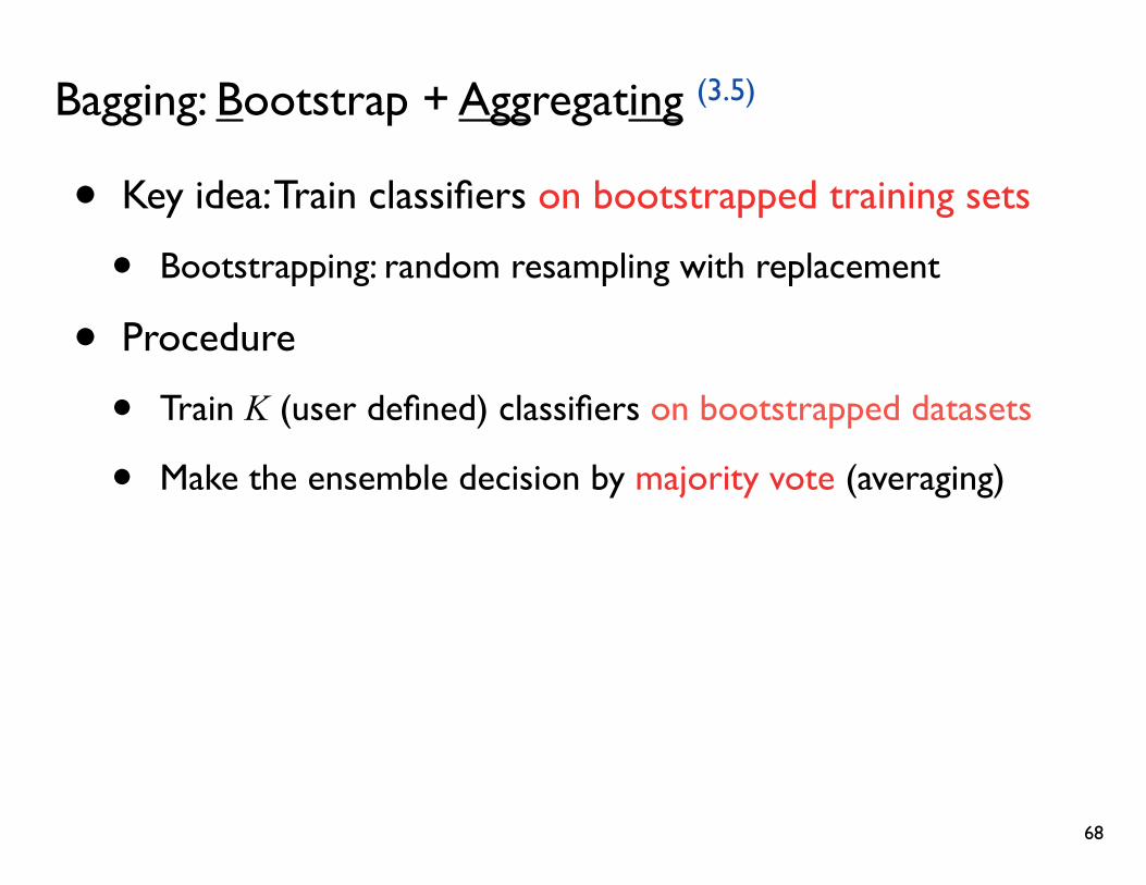
Bagging: Bootstrap + Aggregating (3.5)
• Key idea: Train classifiers on bootstrapped training sets
• Bootstrapping: random resampling with replacement
• Procedure
• Train K (user defined) classifiers on bootstrapped datasets
• Make the ensemble decision by majority vote (averaging)
68

Bagging: Bootstrap + Aggregating (3.5)
• Discuss
+ Good candidate when available data is of limited size
+ Results in a stable model, out of unstable base classifiers
- Does not work (applied to all ensemble methods using majority vote)
- When the accuracy of base classifiers < .5
- When the errors in base classifiers are correlated
69

AdaBoost: Adaptive Boosting (3.6; 3.7)
• Key idea
• Train a series of classifiers focusing on “harder” instances
• On each iteration, instance weights are assigned based on the current ensemble error
• Ensemble decision is made by weight majority vote
• The weights for the base classifiers are obtained after learning
70

AdaBoost: Adaptive Boosting (3.6; 3.7)
• Discuss
+ Has been crowned as the “most accurate off-the-shelf classifiers” [Breiman 1998]
+ A variety of extensions are available (3.7)
- Sensitive to noisy samples or outliers (next slide)
71
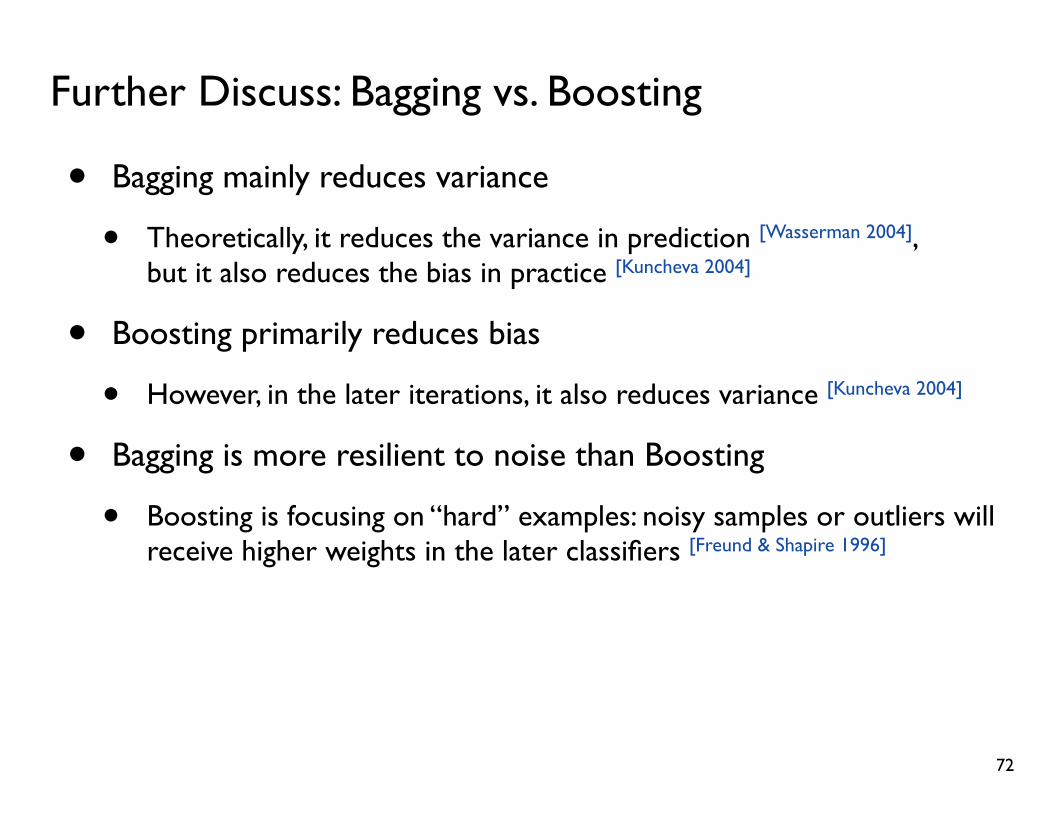
Further Discuss: Bagging vs. Boosting
• Bagging mainly reduces variance
• Theoretically, it reduces the variance in prediction [Wasserman 2004],but it also reduces the bias in practice [Kuncheva 2004]
• Boosting primarily reduces bias
• However, in the later iterations, it also reduces variance [Kuncheva 2004]
• Bagging is more resilient to noise than Boosting
• Boosting is focusing on “hard” examples: noisy samples or outliers will receive higher weights in the later classifiers [Freund & Shapire 1996]
72
Section Agenda
• Ensemble Techniques
✓ Overview
✓ Definition
✓ Motivation
✓ Key Criteria
✓ Popular Techniques
• Ensemble of Multi-dimensional Classifiers
73

Ensembles of Multi-dimensional Classifiers
• Existing methods
• Ensembles of Classifier Chains (ECC) (2.13)
• Ensembles of Probabilistic Classifier Chains (EPCC) (2.16)
• Ensembles of Multi-dimensional Bayesian Net’s (EMBC) (3.10)
• Mixtures-of-Conditional Tree-structured Bayes Net’s (MC) (3.12)
74

Ensemble of Classifier Chains (ECC) (2.13)
• Recall CC (2.13)
• Key idea
• Create multiple CC’s with different random orderings of the class labels
• Predict by simple averaging over all base classifiers
75
Y1 Y2 Y3 Yd...
Ensemble of Classifier Chains (ECC) (2.13)
• Discuss
+ Sometimes, the performance improves
- Ad-hoc implementation
- Learning base classifiers with random ordering
- Ensemble decisions are made by simple averaging
76

Ensembles of Multi-dimensional Classifiers (2.13; 2.16; 3.10)
• Further Discuss
• No principled approaches have been proposed for the ensemble of multi-dimensional classifiers
• Existing methods rely on randomness to generate base classifiers; adopt a simple averaging to make ensemble decisions
• This is somewhat less investigated area
• Research opportunities are here!
77

Section Summary
• Ensemble techniques learn multiple classifiers and combine the predictions of them to produce a better prediction
• Key criteria is accuracy, diversity, and good combining strategy
• Popular ensemble methods have been reviewed
• No principled ensemble method in MDC has been proposed
78

Conclusion
• We discussed MDC, PGM, and Ensemble techniques
• MDC problems formulate the situations where an instance can be associated with more than one class label
• Different approaches are discussed: (1) problem transformation, (2) feature enrichment, (3) output coding, (4) graph-based methods, (5) ensemble-based methods
• PGM offers an efficient way to formulate probability distributions with a large number of random variables
• Ensemble techniques combine simpler learners to improve predictions
79
Conclusion
• PGM and Ensemble Techniques can serve as good implementation methods for MDC
• The main challenge in MDC is that the size of the label space is exponential
• PGM offers methods to discover and exploit the decomposable structures among variables
• Ensemble techniques would give us chances to further improve the prediction accuracy
80

81
Thanks!