a new classification of one-dimensional cellular automata
TRANSCRIPT
A New Classification of One-Dimensional Cellular Automata Using Grossone
Lou D’AlottoDepartment of Mathematics and Computer ScienceYork College, City University of New York andThe Graduate Center, City University of New York
Нижний Новгород, September 2017

The One-Dimensional Plan
• Define and Discuss One-Dimensional Cellular Automata
• Re-Introduce (Recall) The Infinite Unit Axiom and Grossone
• Apply Grossone to Define a new Metric on the Space of One-Dimensional Cellular Automata
• Apply this new Metric and Grossone to Develop a Classification of One-Dimensional Cellular Automata

Infinite Unit Axiom
The number of elements in the set N, of natural numbers is equal to the
infinite unit denoted by
We will give this a name: “Grossone”
1
Introduced in the early part of the 21st century by Yaroslav Sergeyev
Enhances the concept of the unit from finite to infinite.
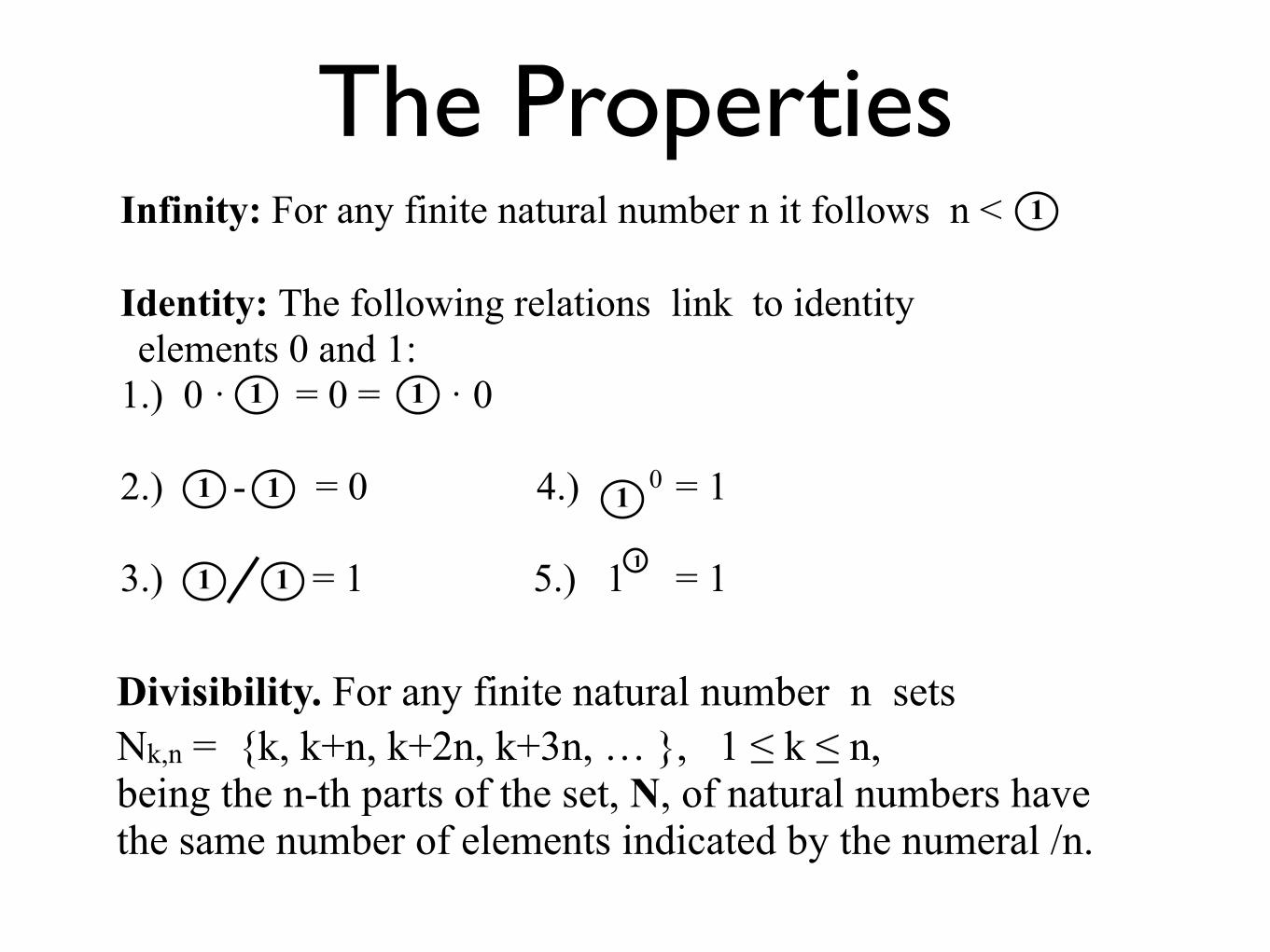
The Properties
Divisibility. For any finite natural number n sets Nk,n = {k, k+n, k+2n, k+3n, … }, 1 ≤ k ≤ n, being the n-th parts of the set, N, of natural numbers have the same number of elements indicated by the numeral /n.
Infinity: For any finite natural number n it follows n <
Identity: The following relations link to identity elements 0 and 1:
1.) 0 · = 0 = · 0
2.) - = 0 4.) 0 = 1
3.) = 1 5.) 1 = 1
1
1 1
1
1 1
1
1
1
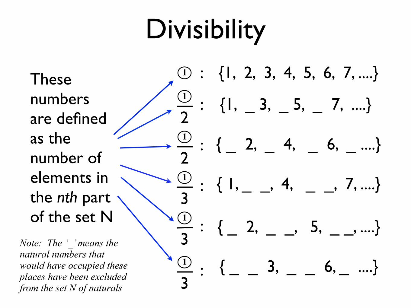
Divisibility
1
2
1 {1, 2, 3, 4, 5, 6, 7, ....}:
: {1, _ 3, _ 5, _ 7, ....}
{ _ 2, _ 4, _ 6, _ ....}1
2:
1
3: { 1, _ _, 4, _ _, 7, ....}
1
3:
{ _ 2, _ _, 5, _ _, ....}1
3:
{ _ _ 3, _ _ 6, _ ....}
These numbers are defined as the number of elements in the nth part of the set N
Note: The ‘_’ means the natural numbers that would have occupied these places have been excluded from the set N of naturals

Some Notes• The new approach does not contradict Cantor, and it
can be viewed as an evolution of his ideas regarding the existence of different infinite numbers in a more applied and precise way.
• The Infinite Unit Axiom introduces a new infinite number, Grossone, and the properties that distinguish it from other numbers.
• - 3, 2 10, 5 2 (-2) 4.2 -2 are all numbers in this new positional infinite base number system.
• Note that -2 is an infinitesimal.
• For example, 2 10 = 2 + 10
1 1 1 1 1
1
1 1

Infinitesimals
• Infinite numbers with parts of the type -i, with i > 0 are called infinitesimals
• Infinitesimals will play an important role in defining a metric and analyzing the forward evolution of cellular automata.
1
Why Not Use The Hyperreals/Infinitesimals?
• Grossone is defined as a number (an infinite number)
• Computation Power
• Grossone, with the defined properties, provides computational power (we have representations of infinite numbers).

Some Important Sets
For further information, please see: http://www.grossone.com/arithmetic.html
1
N, the set of natural numbers, is: {1, 2, 3, 4, ..., -2, -1, }1 1
The set Z, of integers, is:
{- , - +1,...,-2, -1, 0 ,1, 2, 3,..., -2, -1, }1 11 1 1

Extended Sets
The set Z of extended integers is constructed from Z^
This is accomplished the same way as the natural numbers but with additive inverse elements. For example, 2 has as its additive inverse -2 11
The set N of extended natural numbers is formed: ^
{1, 2, ..., -2, - 1, , +1,..., 2 - 1, 2, 2 +1, ...}1 1 1 1 1 1 1
By adding the Infinite Unit Axiom to the axioms of natural numbers
1 < 2 < ... < - 1 < < + 1 < ... < -1, < 2 < ... 1 11
Sure, we have:1 2 1

Number of elements in Some Important Sets
In N, the set of natural numbers, there are elements 1
In the set E, set of evens, there are elements 1
2The same is true for the set of odd numbers.
The set Z, of integers, has 2 + 1 elements1
It can be shown that |Q| = 2 2 + 1 1
For further information, please see: http://www.grossone.com/arithmetic.html
The set Z × Z has (2 +1) * (2 +1) = (2 +1)2
elements or 4 2 + 4 + 1 elements1 1 1
1 1

Cellular Automata
Discrete Systems
Known for their strong modeling properties
Can exhibit self-organizational behavior
Are capable of universal computation
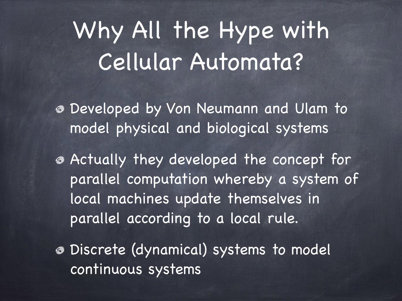
Why All the Hype with Cellular Automata?
Developed by Von Neumann and Ulam to model physical and biological systems
Actually they developed the concept for parallel computation whereby a system of local machines update themselves in parallel according to a local rule.
Discrete (dynamical) systems to model continuous systems

Some ApplicationsUniversal Computation (Turing Machines)
Parallel Computation
Lattice Gas Theory
Forest Fire Models
Lava Flow Models
Cellular and Bacteria Growth Models
Traffic Flow Models

Definitions and Introduction (One-Dimensional)
An alphabet S of size greater than 1
For example, S = {0,1} (the binary alphabet)
Use the one-dimensional integer lattice Z and let X = SZ
The space of all maps x: Z → S
Or the space of all bi-infinite sequences of elements of S
The setting
(la regolazione)

One-Dimensional Cellular Automata Maps
One-dimensional cellular automata are induced by arbitrary maps (local rule): F: S(2r+1) → S
r ∈ N ∪ {0} is called the range of the map.
The automaton map f induced by F is defined by f(x) = y with y(i)=F(x[i-r],...,x[i],...,x[i+r])

One-Dimensional Neighborhoods
A neighborhood ofrange r = 1
A cell in the next generation
A neighborhood ofrange r = 2
x(i-2) x(i+2)x(i)x(i)

A Configuration
x(-2) x(2)x(0)
... ...
x(-1) x(1)
......
Defined on the integers, Z: The initial configuration
f
The first iteration (application) of the automaton local rule F, in parallel
......
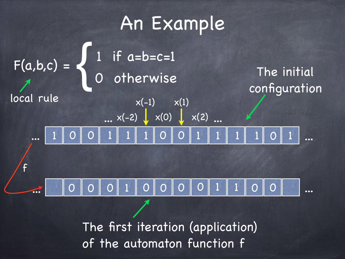
An Example
x(-2) x(2)x(0)
... ...
x(-1) x(1)
......
The initial configuration
f
The first iteration (application) of the automaton function f
......
01 10 1 1 111001 0 1
1000 0 0 0 0 1 1 0 0
F(a,b,c) = { 1 if a=b=c=10 otherwise
local rule

Some Interesting Cellular Automata Rules and their Forward Evolution
Initial Random Configurations
Forward Iterations (Evolution)
A Dynamical Process
• Cellular Automata produce a dynamic process (Discrete) -an evolutionary (iterative) process
• Hence it is interesting to study the long term effects of these processes.
• 1980s : Stephen Wolfram studied the forward dynamics of one-dimensional cellular automata
• Noticed that different configurations behave differently under different automata rules.
• However, if the configuration is chosen at random, the probability is high that the CA will fall into one of 4 classes

A Dynamical Process (formal definition)
The set N of natural numbers = {1, 2, 3,...., - 1, }1 1
The set N0 = {0,1, 2, 3,...., - 1, } 1 1
The ith iterate of a function (automaton function) is the sequence: f i(x) = f ∘ f ∘ f ∘ f ∘ f ... ∘ f(x) where 0 ≤ i ≤ 1
Theorem: The number of elements of any infinite sequence is less than or equal to 11
1 Sergeyev, A new Applied Approach for executing computations with infinite and infinitesimal quantities, Informatica 19 (4) (2008) 567-596

Wolfram Classes
• Class 1: Evolution tends to a spatially homogeneous state
• Class 2: Evolution yields simple stable or periodic structures
• Class 3: Exhibits chaotic aperiodic behavior
• Class 4: Yields complex localized structures, some propagating
Partitioned one-dimensional CA into 4 classes based on their observed dynamical behavior:

Some Cellular Automata Rules
Wolfram Class I Rule 36
Wolfram Class 2Rule 24
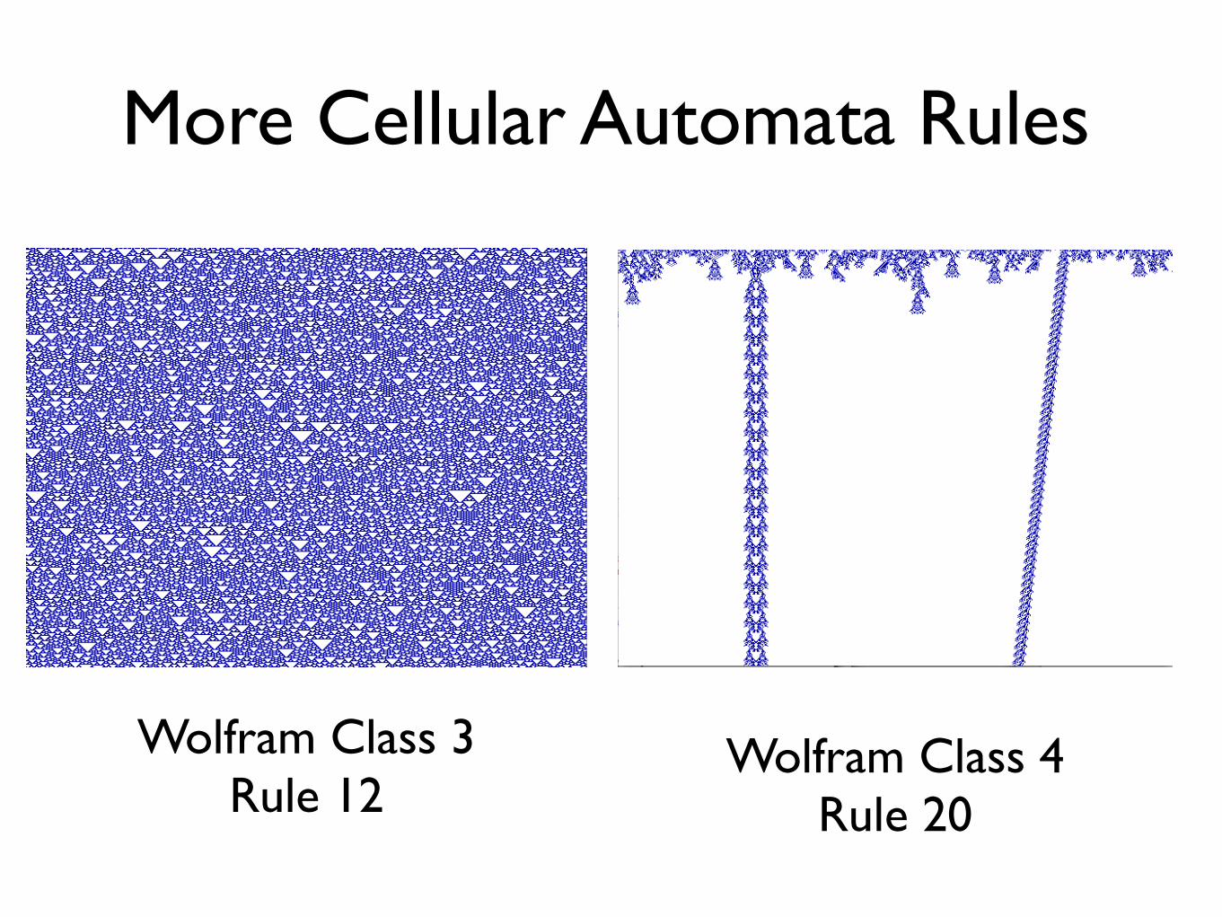
More Cellular Automata Rules
Wolfram Class 3Rule 12
Wolfram Class 4Rule 20
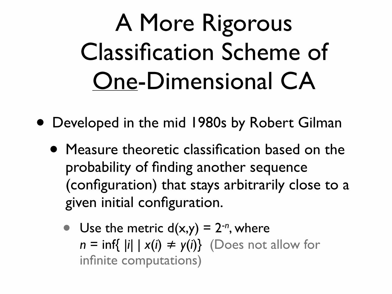
A More Rigorous Classification Scheme of One-Dimensional CA
• Developed in the mid 1980s by Robert Gilman
• Measure theoretic classification based on the probability of finding another sequence (configuration) that stays arbitrarily close to a given initial configuration.
• Use the metric d(x,y) = 2-n, where n = inf{ |i| | x(i) ≠ y(i)} (Does not allow for infinite computations)
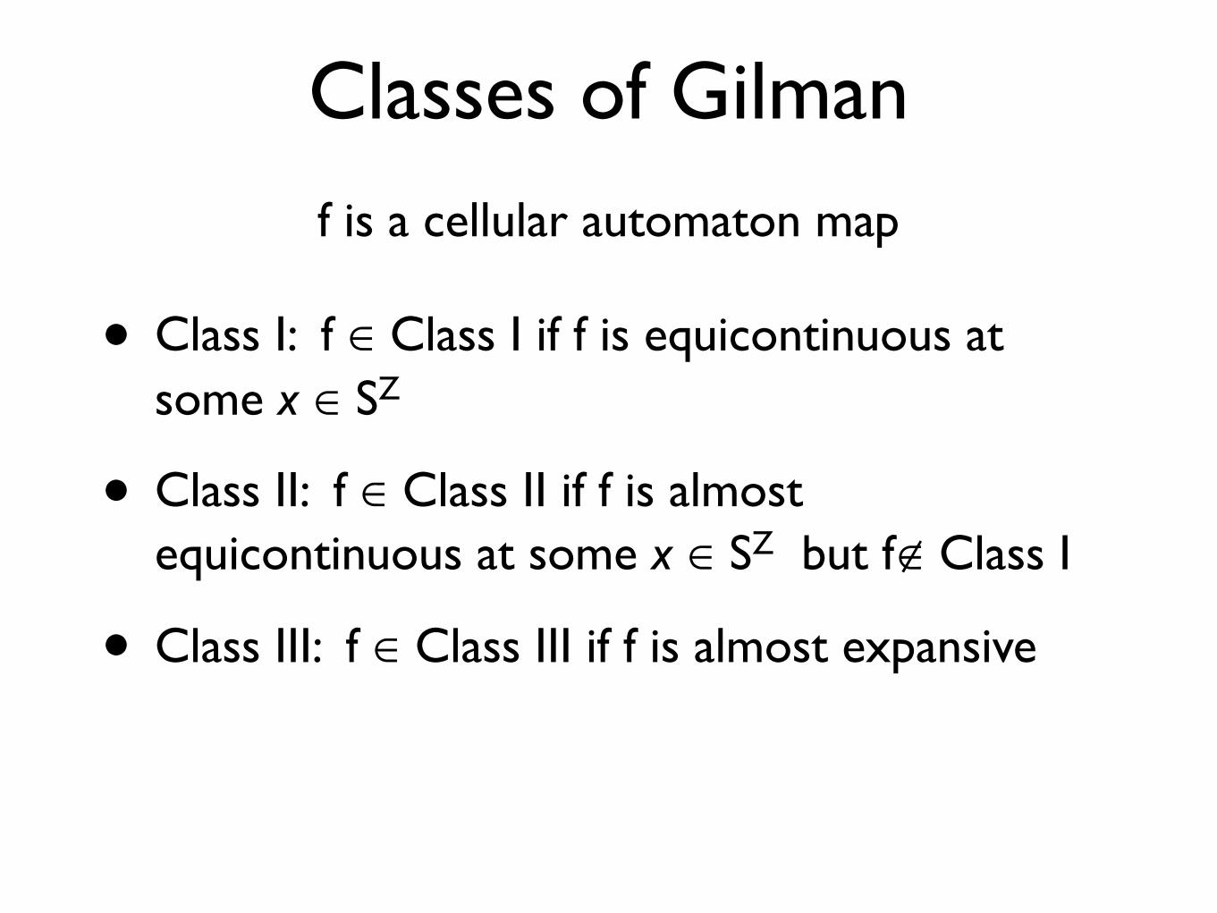
Classes of Gilman
• Class I: f ∈ Class I if f is equicontinuous at some x ∈ SZ
• Class II: f ∈ Class II if f is almost equicontinuous at some x ∈ SZ but f∉ Class I
• Class III: f ∈ Class III if f is almost expansive
f is a cellular automaton map
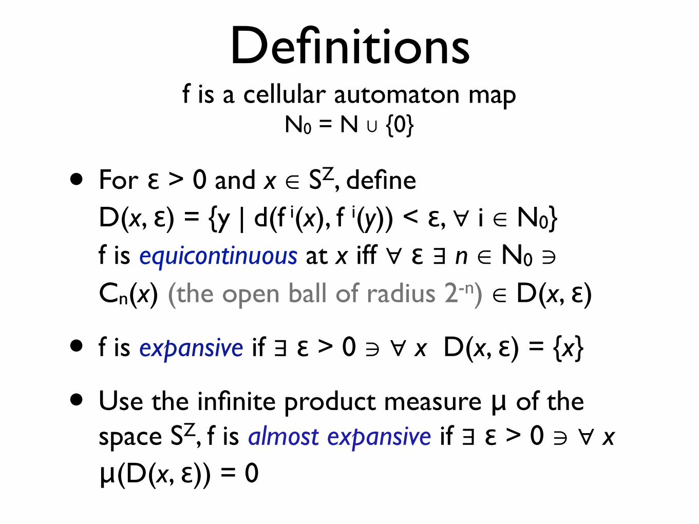
Definitions
• For ε > 0 and x ∈ SZ, define D(x, ε) = {y | d(f i(x), f i(y)) < ε, ∀ i ∈ N0} f is equicontinuous at x iff ∀ ε ∃ n ∈ N0 ∋ Cn(x) (the open ball of radius 2-n) ∈ D(x, ε)
• f is expansive if ∃ ε > 0 ∋ ∀ x D(x, ε) = {x}
• Use the infinite product measure μ of the space SZ, f is almost expansive if ∃ ε > 0 ∋ ∀ x μ(D(x, ε)) = 0
f is a cellular automaton mapN0 = N ∪ {0}

Definition of Almost Equicontinuous
f is almost equicontinuous at x iff ∀ ε > 0
lim μ(Cn(x) ∩ D(x, ε)) μ(Cn(x))
n → ∞ = 1
Gilman goes on to define some properties of these classes but does not provide an algorithm for membership.Class III does not distinguish between countable and uncountable
A Few Notes:

A New Classification Based on Grossone
• Does not Involve Measure Theory (The Lens of Measure Theory is limited in distinguishing infinite sets).
• Uses Grossone to count the number of elements in the set of elements that follows, under forward iteration, that of a given initial sequence (stays close to under the metric).

The Domain Space of Cellular Automata
Recall S is a finite alphabet, for example S = {0,1}And SZ is the space of all bi-infinite sequences defined on the integers and taking values from S
Theorem: |SZ | = |S|2 + 11
Hence we know the number of bi-infinite sequences in the entire spaceThis is extremely interesting and important since, via Cantor, this space is considered uncountable!
As usual, let |Y| = the number of elements in the set

The Metric
x ⋀ y = {Let x and y be two bi-infinite sequences in SZ
x
*x(-n)...x(0)...x(n) if x(i) = y(i) ∀i ∈ [-n,n] and *
outside
if x(0) ≠ y(0) or x(0) = *if x = y
Note, -n can be infinite and equal - + k and n can equal - k for some finite integer k ≥ 0 Also note in this case, if k = 0, then x = y.
1
1
Hence we can do computations on infinite wordsNote, x ⋀ y is the largest center stretch where x and y agree
Lower unitinfimum operation
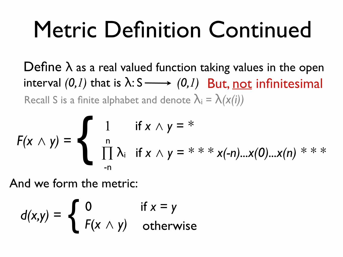
Metric Definition ContinuedDefine λ as a real valued function taking values in the open interval (0,1) that is λ: S (0,1) But, not infinitesimal
F(x ⋀ y) = { 1 if x ⋀ y = *
∏ λi n
-nif x ⋀ y = * * * x(-n)...x(0)...x(n) * * *
Recall S is a finite alphabet and denote λi = λ(x(i))
And we form the metric:
d(x,y) = { 0F(x ⋀ y)
if x = y otherwise

Some Notes
• It is a simple exercise to check this is a metric on the space SZ
• This metric satisfies the nonarchimedean or ultra metric inequality
• Great advantage using Grossone: we can use configurations that agree on infinite intervals, and are infinitesimally close to each other.
d(x,y) ≤ max{d(x,z), d(z,y)}

Open SetsC(-n,n,x[-n,n]) = {x ∈ SZ | x[-n,n] = w}, where |w| = (2n+1)}
The disk of radius ε around x is C[-n,n](x) = C(-n,n,x[-n,n])
Note n is a natural number -n ≤ 0 ≤ n and possibly infinite.
A quantity w = x[-n,n] represents a word in the interval [-n,n] and of length 2n+1.
It is allowable for n to be an infinite number, for example - k, where k is some natural number.1
In this case we obtain an open disk of infinitesimal radius
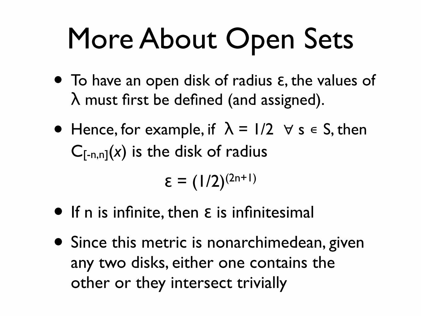
More About Open Sets• To have an open disk of radius ε, the values of λ must first be defined (and assigned).
• Hence, for example, if λ = 1/2 ∀ s ∊ S, then C[-n,n](x) is the disk of radius
• If n is infinite, then ε is infinitesimal
• Since this metric is nonarchimedean, given any two disks, either one contains the other or they intersect trivially
ε = (1/2)(2n+1)

And Still More
Theorem: |SZ | = |S|2 + 11
Recall:
Corollary: The open disk C[-n,n](x) around x contains
|S|2( - n)1Elements
Proof: Follows directly from the Theorem
n = 22-2 0
1 -21 -2
* *** ** * * *... ...*|S|( - 2)1 |S|( - 2)1
-1 1
|S|2( - n)1 choiceschoices

Classes of One-Dimensional CA
• Necessary to Study the Forward Iterates of the CA function.
• Will allow us to compute how many (now possible with Grossone) configurations equal or match that of a given initial configuration.
Understanding the Dynamics

Let’s Do it!Define: Bm,n(x) = {y | f i(y)[m,n] = f i(x)[m,n] ∀i ∈ N0, m≤0≤n}
Recall: f i(y)[m,n] represents the ith iteration of a word, around (not necessarily centered) the 0 position. That is, a center window. Note that the CA function f is first applied to the entire configuration x (or y) and then restricted to the interval [m,n]Also Note that, due to the Infinite Unit Axiom, m can equal - +k and, similarly, n can equal -k for some finite integer k ≥0 (not necessarily the same value k).
1 1

Hence• The Dynamical Analysis of Cellular
Automata presented herein is based on using the Infinite Unit Axiom to count the number of elements in the Bm,n classes.
• This gives us the precise number of configurations that will equal an initial configuration upon forward evolution (iteration) of the CA function.
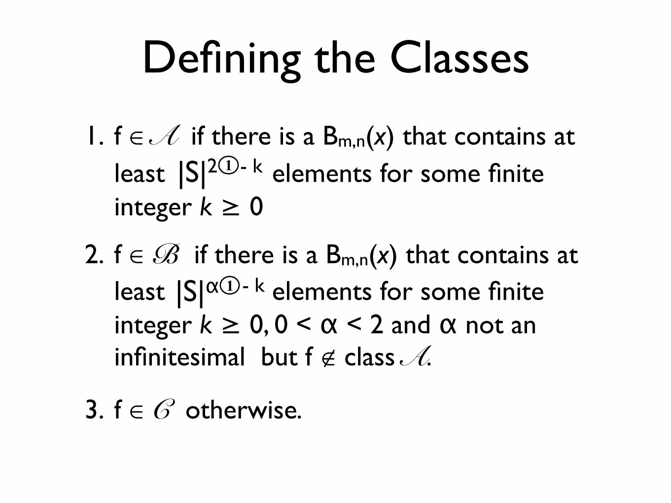
Defining the Classes
1. f ∈ A if there is a Bm,n(x) that contains at least elements for some finite integer k ≥ 0
2. f ∈ B if there is a Bm,n(x) that contains at least elements for some finite integer k ≥ 0, 0 < α < 2 and α not an infinitesimal but f ∉ class A.
3. f ∈ C otherwise.
|S|2 - k1
|S|α - k1

Two Resulting Theorems
Theorem A: If there exists a Bm,n(x), for cellular automaton f, that contains a disk of non-infinitesimal radius, then f ∈ A
Theorem B: If f ∈ A then there exists a Bm,n(x) class that contains a disk (of non-infinitesimal radius).
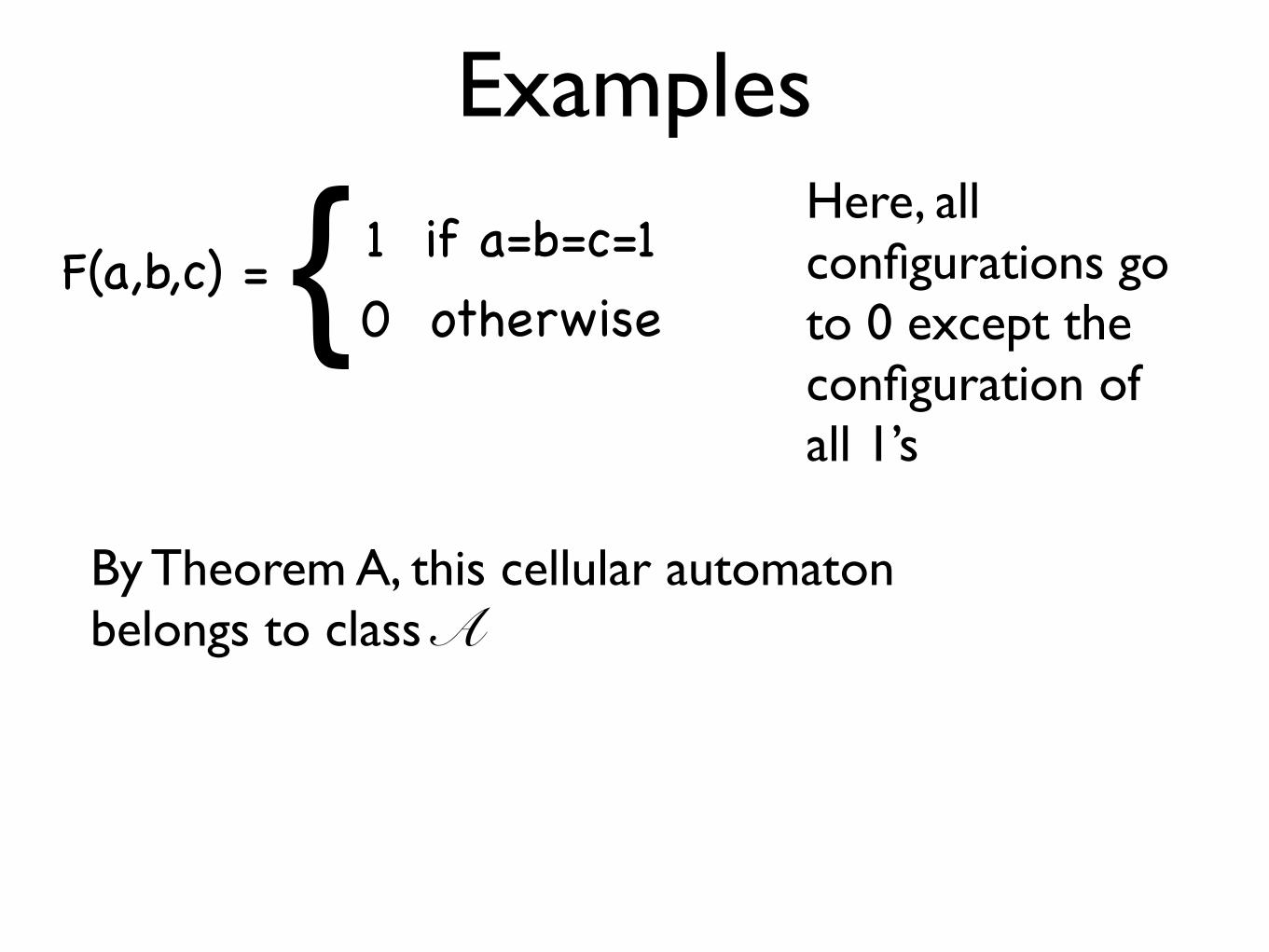
Examples
F(a,b,c) = { 1 if a=b=c=10 otherwise
Here, all configurations go to 0 except the configuration of all 1’s
By Theorem A, this cellular automaton belongs to class A
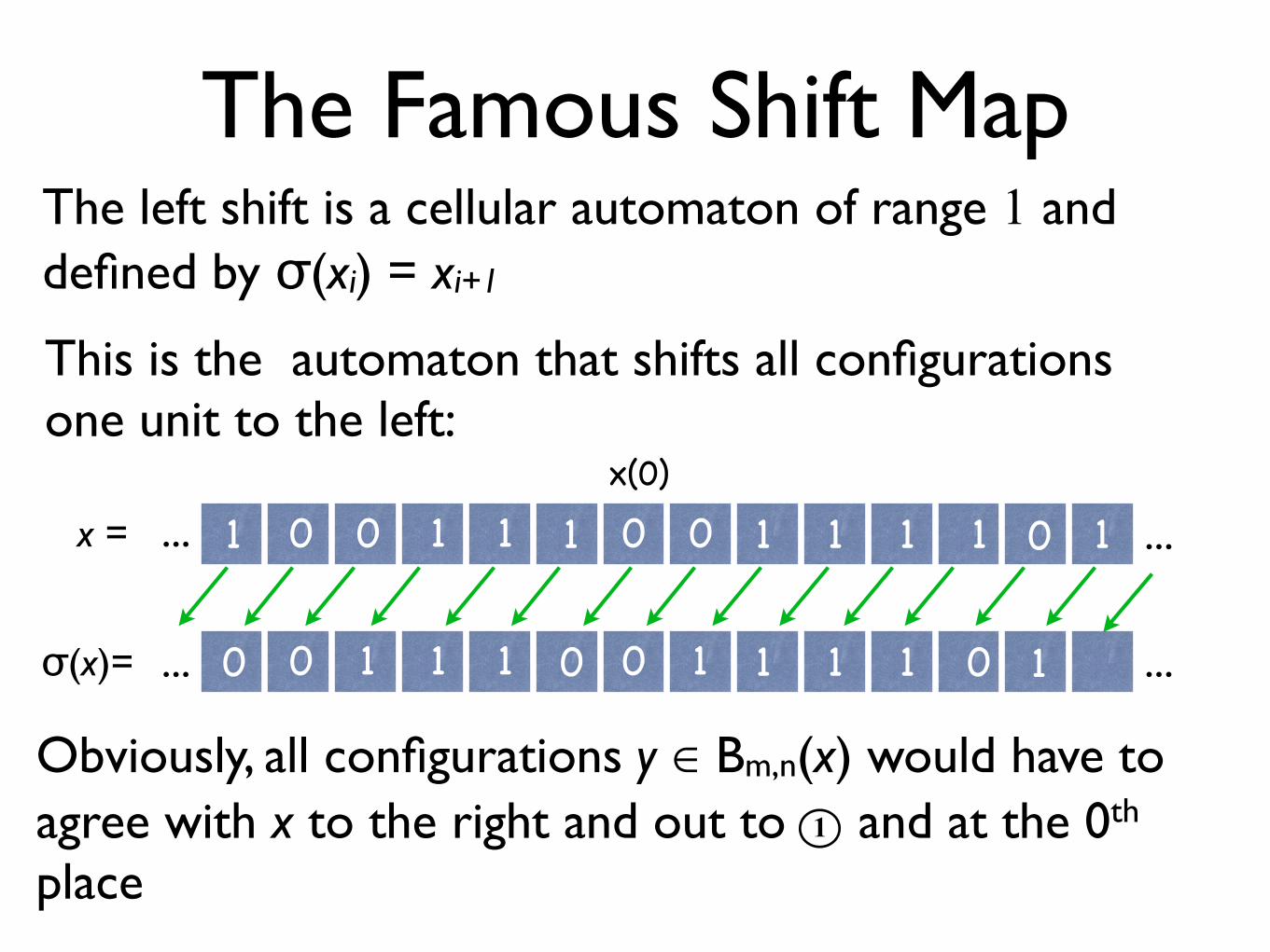
The Famous Shift MapThe left shift is a cellular automaton of range 1 and defined by σ(xi) = xi+1
This is the automaton that shifts all configurations one unit to the left:
01 10 1 1 111001 0 1x(0)
σ(x)= 00 11 1 1 011100 1
x =
...
...
...
...
Obviously, all configurations y ∈ Bm,n(x) would have toagree with x to the right and out to and at the 0th
place1

The Shift Map Continued
Hence, there are at most elements, for some k ≥ 0 in any Bm,n(x) and σ must be in Class B.
Since all configurations y ∈ Bm,n(x) would have toagree with x to the right and out to and at the 0th place:
1
|S| - k1

Modulo Sum RulesModulo sum (Additive Cellular Automata)
F(a,b,c) = (b+c) mod 2
Some examples for the binary alphabet S = {0,1}:
F(a,b,c) = (a+c) mod 2
a cb
a b c
Range = 1
Again, Range = 1
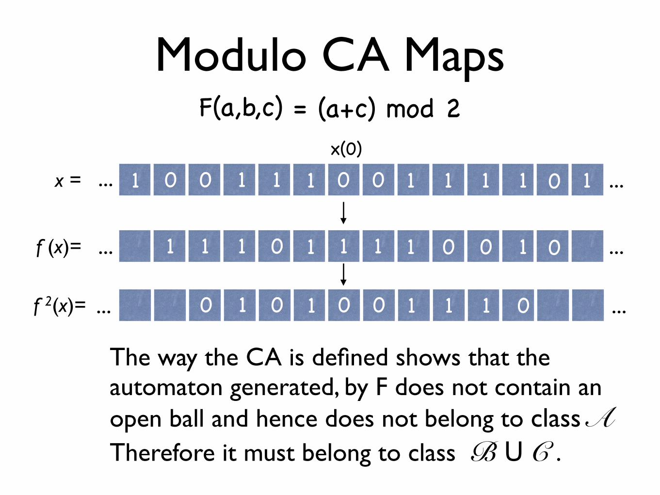
Modulo CA MapsF(a,b,c) = (a+c) mod 2
01 10 1 1 111001 0 1x(0)
f (x)= 11 11 0 0 10111 0
x =
...
...
...
...
01 10 1 1 0010f 2(x)= ... ...
The way the CA is defined shows that the automaton generated, by F does not contain an open ball and hence does not belong to class A Therefore it must belong to class B U C .

And .... Future Work
• Construct an example(s) of a Class 3 cellular automata. Possibly show that the modulo 2 rule does not belong to class B. Another possible example would be a cellular automata that exhibits universal computation, such as Wolfram rule 1501
• Develop a finer distinction of classes using Grossone
• Develop an algorithm for membership in each of these classes.
1 See Wolfram, S., A New Kind of Science