monte carlo methods for radiative transfer with singular...
TRANSCRIPT

Monte Carlo methods for radiative transfer withsingular kernels
Christophe Gomez, ∗,1 and Olivier Pinaud †2
1Aix Marseille Universite, CNRS, Centrale Marseille, I2M, UMR 7373,13453 Marseille, France
2Department of Mathematics, Colorado State University, Fort CollinsCO, 80523
May 15, 2017
AbstractThis work is devoted to Monte Carlo methods for radiative transfer equa-
tions with singular kernels, and is motivated by the study of wave propagation inrandom media with long-range dependence. As opposed to the short-range casewhere the collision cross section is integrable and leads to a non-zero mean freetime, the cross section is not integrable in the long-range situation and yields avanishing mean free time. For computational efficiency, a particular care is thenrequired in the construction of the stochastic processes used in the Monte Carlomethods. For this, we adapt a method of Asmussen-Rosinski and Cohen-Rosinskibased on a small jumps/large jumps decomposition of the generator. We comparethis method with another approach based on alpha-stable processes, and show thesuperiority of the first one. We consider various algorithms for the simulation ofthe jump distribution, and underline the efficiency of an appropriate stochasticcollocation method. Comparisons between integrable and singular kernel solutionsare given.
1 Introduction
This work is devoted to the derivation of Monte Carlo methods for the resolution oftwo-dimensional radiative transfer equations (RTE) of the form
∂tf + k · ∇xf = Q(f), f(t = 0) = f0, (x, k) ∈ R2 × S1, (1)
with collision operator
Q(f)(k) =
∫S1
F (k · p)(f(p)− f(k))dσ(p), F ≥ 0.
∗[email protected]†[email protected]
1
Above, σ(p) is the surface measure on S1. Our motivation comes from the study of highfrequency wave propagation in random media. In such a context, the function f solutionto the RTE describes the wave energy density in the phase space, see [12, 19, 28, 31]for a few references. The collision term models the interaction between the wave andthe fluctuations of the underlying medium in the so-called weak coupling regime. Forinstance, if c(x) is the velocity field and reads
1
c(x)2=
1
c20(1 + V (x)) ,
where c0 is a constant background velocity and V is a mean zero, stationary randomfield that models fluctuations around the background, then the collision kernel F isproportional to the Fourier transform of the correlation function
R(x− y) = E{V (x)V (y)}.
The symbol E means expectation over realizations of the random medium, and thekernel F is nonnegative by application of Bochner theorem.
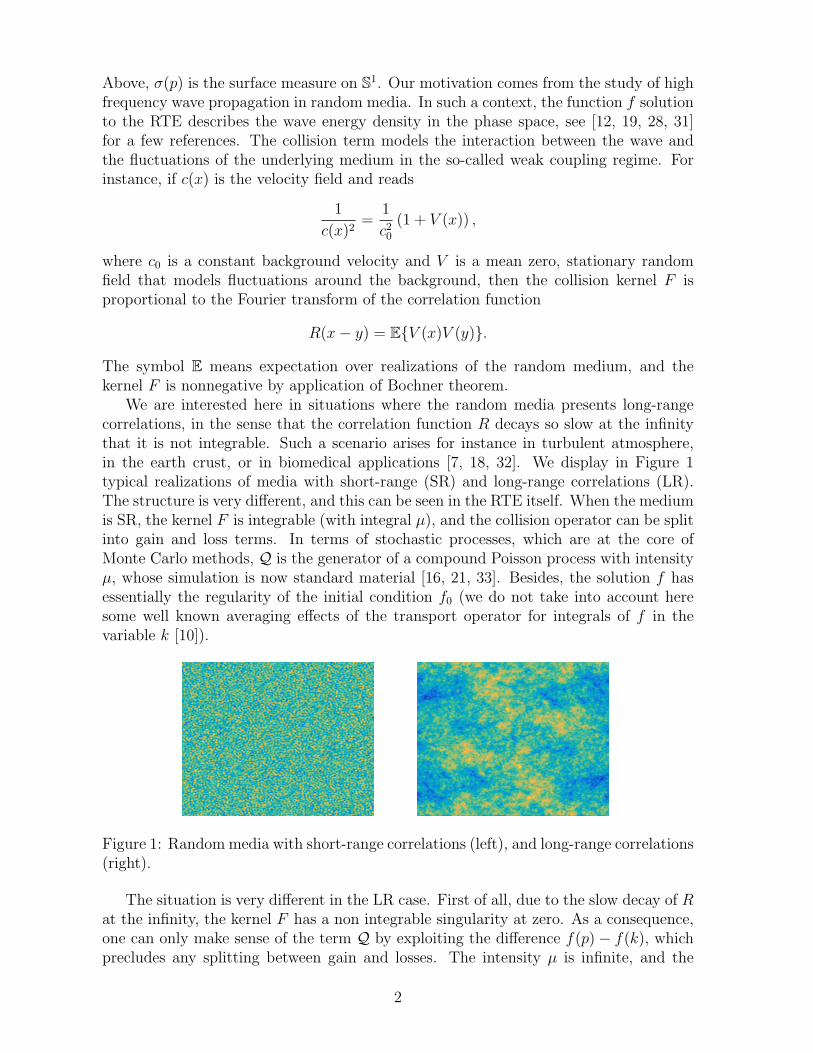
We are interested here in situations where the random media presents long-rangecorrelations, in the sense that the correlation function R decays so slow at the infinitythat it is not integrable. Such a scenario arises for instance in turbulent atmosphere,in the earth crust, or in biomedical applications [7, 18, 32]. We display in Figure 1typical realizations of media with short-range (SR) and long-range correlations (LR).The structure is very different, and this can be seen in the RTE itself. When the mediumis SR, the kernel F is integrable (with integral µ), and the collision operator can be splitinto gain and loss terms. In terms of stochastic processes, which are at the core ofMonte Carlo methods, Q is the generator of a compound Poisson process with intensityµ, whose simulation is now standard material [16, 21, 33]. Besides, the solution f hasessentially the regularity of the initial condition f0 (we do not take into account heresome well known averaging effects of the transport operator for integrals of f in thevariable k [10]).
Figure 1: Random media with short-range correlations (left), and long-range correlations(right).
The situation is very different in the LR case. First of all, due to the slow decay of Rat the infinity, the kernel F has a non integrable singularity at zero. As a consequence,one can only make sense of the term Q by exploiting the difference f(p)− f(k), whichprecludes any splitting between gain and losses. The intensity µ is infinite, and the
2

operator Q is now the generator of a general Levy process on S1, and not just of a purejump Poisson process as in the SR case. Informally, µ−1 measures the average timebetween collisions (the “Mean Free Time”), which means in the LR case that collisionsare taking place in a continuous basis. The simulation of such Levy processes in thecontext of transport equations seems much less studied than its compound Poissoncounterpart, and is then the object of this work. We focus here on the two-dimensionalcase with velocities on S1, and will address the three-dimensional case elsewhere. Notethat the choice of S1 is arbitrary, any circle of given radius would be dealt with inthe same fashion. The singularity of kernel tends to favor grazing collisions, and as aconsequence this LR regime bears some strong similarities with the classical peaked-forward regime [20, 23, 25], with the forward effect magnified by the singularity.
Regarding the regularity of f , it was established in [13, 14] that f is C∞ in allvariables for all t > 0, which is in stark contrast with the SR case. The regularity isreminiscent of the hypoelliptic nature of (1) when F is not integrable. Our originalmotivation for studying (1) is the resolution of some inverse problems, for instancethe localization of sources or inclusions in clutter. Since inversion techniques based ontransport equations are often based on the singularities of f , see [3], the smoothness off indicates that the inversion, if possible at all, should be more difficult than in the SRsituation.
Monte Carlo (MC) methods have several advantages compared to classical finiteelements or finite volumes methods. They can handle the high-dimensionality of (1) ina simple manner, since no mesh is required and the quantity of interest only need bediscretized at a detector where measurements take place. They are very flexible in termsof geometry, provided the boundary conditions on f can be translated into boundaryconditions on the underlying stochastic process, and are generally applicable when thecoefficients in the equation depend on the variables (x, k). MC methods are also veryeasy to implement and can be parallelized in a straightforward manner, which is a strongfeature with today’s technology. Note that discretization-based methods would have tohandle carefully the singularity of the cross-section.
On the down side, while MC methods offer a relatively good accuracy at low cost,getting more accurate results can come at a significant increase in the computationaltime. Some variance reduction techniques might then be necessary to lower this cost.
Typical collisions kernels in turbulent atmosphere are the celebrated Kolmogorov(K) power spectrum [27], or its Von Karman (VK) variant including the inner and outerscales of the turbulence [26]. With F (k, p) = Φ(|k − p|), they read
Φ(|k|) = C0|k|−113 (K), Φ(|k|) = C1(1 + L2
0|k|2)−116 e−`
20|k|2 , (VK),
where C0 and C1 are constants, and L0, `0 are the outer and inner scales, respectively.In a turbulent regime, we have L0 � `0, so that the Von Karman power spectrumbehaves like the Kolmogorov power spectrum at k = 0, and is therefore not integrablein dimensions two and three. In this work, we will mostly focus on kernels of the formF (k ·p), and explain how our methods can be directly adapted to kernels like F (x, k, p).We consider kernels with power singularities such as the Kolmogorov power spectrum,that read
F (k · p) =A(k · p)|k − p|1+α
, α ∈ (0, 2), 0 < a ≤ A(s) ≤ a <∞, (2)
3

for s ∈ [−1, 1].With the hypotheses above, the operator Q can be seen the generator of a Levy
process (Kk(t))t≥0 on S1, with initial condition Kk(0) = k, see [13]. Introducing theposition
Xx(t) = x+
∫ t
0
Kk(s)ds,
the solution f to (1) is then
f(t, x, k) = E{f0(Xx(t), Kk(t))}.
GeneratingN independent copies (Xxi , K
ki )i=1,...,N of the random trajectories (Xx(t), Kk(t))t≥0,
f is approximated by the empirical average
fN(t, x, k) =1
N
N∑i=1
f0(Xxi (t), Kk
i (t)),
while the central limit theorem shows that the error is controlled by some measure ofthe standard deviation of fN divided by
√N .
The key to MC methods is an efficient simulation of the process (K(t))t≥0. Tothis end, we adapt a method of the probabilistic literature developed by Asmussen-Rosinski [1], and Cohen-Rosinski [6], that we will refer to as the ACR method. Theidea is to introduce a cut-off in the collision operator to remove the singularity. Theresulting operator is then the generator of a compound Poisson process with finite (butlarge) intensity. The issue is that a small value of the cut-off parameter is required forgood accuracy, leading to a high intensity and therefore to many collisions increasingthe computational time. The issue is fixed by adding a correcting term describingasymptotically the behavior of the operator around the singularity. This term modelsfrequent jumps of small amplitude, while the regularized generator describes more rarejumps with larger amplitudes. In the work of Asmussen-Rosinski, and Cohen-Rosinski,the correction takes the form of a Brownian motion on the real line, while in our casewe obtain a Brownian motion on the circle (more generally we would obtain a Brownianmotion on Sd with generator given by the Laplace-Beltrami operator on Sd).
Without another MC method to compare against, the efficiency of the ACR methodfor the simulation of transport equations is not obvious at first since it is only anapproximation and the cost of the generation of a compound Poisson process with largeintensities is to be determined. To this goal, we carefully design an alternative MCmethod that does not involve a regularization of the generator, and is based on the so-called alpha-stable processes. We will refer to this second method as the AS method. Wealso derive an efficient way to simulate the jump distribution of the compound processthat accounts for the singularities of the kernel, and is based on the stochastic collocationmethod. We show that the ACR method is very efficient and, perhaps surprisingly, thatit is superior to the AS method for both weakly singular kernels (i.e. α close to 0) andhighly singular kernel (α close to 2).
The paper is organized as follows. In Section 2, we present the ACR method andgive an error analysis. We introduce the AS method in Section 3 and Section 4 is de-voted to algorithms for the jump distributions. We describe rejection sampling methodsand the stochastic collocation method. We perform simulations in section 5, and start
4

by comparing the latter methods, and show the superiority of the last one. We thenaddress the impact of the Brownian correction in the ACR method, and compare theperformances of ACR and AS methods. We also investigate the sensitivity of the ACRmethod to the cut-off parameter. We conclude the simulations section by comparing thesolutions to the RTE for underlying random media with SR and LR correlations, andby investigating the role of the function a. We finally present generalizations to kernelsof the form F (x, k, p) in Section 6, and a conclusion is offered in Section 7.
Acknowledgment. OP is supported by NSF CAREER grant DMS-1452349.
2 The ACR method
We adapt in this section the method introduced by Asmussen-Rosinski in [1] and Cohen-Rosinski in [6]. For this, we need first to appropriately parametrize the operator Q. Thenatural choice for Q are the polar coordinates and we introduce the surjective map
P : φ ∈ R 7−→ (cos(φ), sin(φ)) ∈ S1.
Setting k = (cos(θ), sin(θ)) and p = (cos(θ′), sin(θ′)) so that k · p = cos(θ′ − θ), andrewriting
A(k · p) = a(θ′ − θ),
the collision kernel Q can be recast as
Q(f)(k) =1
21+α
2
∫ π
−π
a(θ′ − θ)(f(θ′)− f(θ))
(1− cos(θ′ − θ)) 1+α2
dθ′
=1
21+α
2
∫ π
−π
a(θ′)(f(θ′ + θ)− f(θ))
(1− cos(θ′))1+α
2
dθ′
= Q(f)(θ), θ ∈ [−π, π],
where f = f ◦ P is a 2π-periodic function. Note that the 2π-periodic function a issymmetric with respect to 0 and is nonnegative. The operator Q can be seen as thegenerator of a Levy process on [−π, π] starting from 0, that we denote by (Θ(t))t≥0.According to our parametrization,
(Kk(t))t≥0 = (P (Θ(t) + θ))t≥0 in law.
For ε ∈ (0, 1), the ACR method consists in splitting Q into
Q(g)(θ) = Qε<(g)(θ) +Qε>(g)(θ)
:=1
21+α
2
∫ICε
a(θ′)(g(θ′ + θ)− g(θ))
(1− cos(θ′))1+α
2
dθ′ +1
21+α
2
∫Iε
a(θ′)(g(θ′ + θ)− g(θ))
(1− cos(θ′))1+α
2
dθ′
where Iε is the setIε := {θ′ ∈ [−π, π], | tan(θ′/4)| > ε/4} ,
5

and ICε its complementary in [−π, π]. The reason for the latter form of the cut-off willbe apparent further. Because of the regularization, the second piece of the generator,namely Qε>(g), is now the generator of a classical compound Poisson process with jumpintensity
µε =Π0ε
21+α
2
, where Π0ε =
∫Iε
a(θ)dθ
(1− cos(θ))1+α
2
,
and jump distribution
Πε(dθ) =1Iε(θ)a(θ)
Π0ε(1− cos(θ))
1+α2
dθ.
The expected number of jumps for the compound Poisson process in any time interval[0, T ] is given by µεT . The term µε blows up as ε → 0, we will give a precise estimatefurther, and this fact is the reason for the need of an efficient simulation technique forthe jump distribution.
The first term of the generator, i.e. Qε<, models frequent jumps of small amplitude
and can be asymptotically reduced to the generator of a Brownian motion on the circleas explained in the next section.
2.1 The generator Qε<
We have the following lemma, proved in Appendix A.1, which describes the relationbetween Qε< and the Laplace operator.
Lemma 2.1 Suppose that a ∈ C2([−π, π]) and that g is a smooth 2π-periodic boundedfunction with bounded derivatives. Then, for any φ ∈ [−π, π],
Qε<(g)(φ) =Dε
2
∂2g(φ)
∂φ2+Rε[g](φ),
where
Dε =2a(0)ε2−α
2− αand ‖Rε[g]‖∞ ≤
ε4−α
4− α‖a‖C2([−π,π])‖g‖C4([−π,π]).
The leading term in Qε< is the generator of a Levy process with density
pεB(t, φ) =1
2π+
1
π
∞∑`=1
e−tDε`2/2 cos `φ, t > 0.
It can be directly simulated by remarking that, using the Poisson summation formula,
pεB(t, φ) =1√
2πtDε
∑`∈N
e−(2π`+φ)2
2tDε , t > 0,
which, if φt is a centered Brownian motion with variance tDε, is the density of (φtmod 2π). Brownian trajectories starting from 0 can easily be generated using the fol-lowing relation :
φεnh = φεnh − φε(n−1)h + · · ·+ φε2h − φεh + φεh
:= Xn + · · ·+X2 +X1,
6

where (Xi)i=1,...,n are i.i.d centered Gaussian random variable with variance hDε, thatwe denote by N (0, hDε). Note that Dε is proportional to ε2−α/(2− α), which becomeslarger as α increases. We therefore expect the inclusion of the Brownian term in thesimulation to be critical in order to obtain good accuracy and computational cost.
2.2 The generator Qε>
As already mentioned, this operator is the generator of a compound Poisson processwith Levy measure µεΠε. Denoting by (θε(t))t≥0 such a process starting at 0, a samplepath has the form
θε(t) =Nt∑i=1
θi, (3)
where (Nt)t≥0 is a Poisson process with intensity µε, independent of (θi)i≥1, which is asequence of i.i.d random variables distributed according to Πε(dθ). The sojourn timesin each state i are independent and satisfy an exponential distribution with parameterµε.
In order to simulate the process, we use the following parametrization. Since thejump distribution Πε(dθ) is symmetric around the origin, we can write θ = sign(θ)|θ| :=sθθ′, where sθ takes the values ±1 with equal probability, and θ′ ∈ Iε,+ := Iε ∩ [0, π].
We then rewrite Πε asΠε(dθ) = πε(θ
′)dθ′dµ(sθ),
with
dµ(sθ) =1
2(δ(sθ + 1) + δ(sθ − 1)) , πε(θ
′) =1Iε,+(θ′)a(θ′)
Π0ε,+(1− cos(θ′))
1+α2
,
and
Π0ε,+ =
∫Iε,+
a(θ)dθ
(1− cos(θ))1+α
2
. (4)
Therefore, in order to simulate a jump θ under Πε(dθ), we generate θ′ according toπε(θ
′)dθ′, and multiply it by sθ = ±1 with equal probability.Note that the rate µε satisfies the asymptotics
µε 'ε→0
a(0)
2αεα, (5)
and therefore blows up as expected in the limit ε→ 0. This expresses the fact that theprocess jumps more and more as ε becomes small, which hence increases the simulationcost. Note also that the rate blows up more rapidly when α is large. Several methodsto simulate πε will be presented in Section 4.
2.3 Error analysis
The main idea of the ACR method is that the Levy process (Kk(t))t≥0 on S1 startingat k with generator Q is approximated by the process
(Kk,ε(t))t≥0 =((cos(φε(t) + θε(t) + θ), sin(φε(t) + θε(t) + θ)
)t≥0,
7

where φε and θε, defined in the last two sections, are independent. Note that we replacedφε mod 2π by φε by periodicity. The process (φε(t))t≥0 is generated as described inSection 2.1, while (θε(t))t≥0 has the form (3).
With
Xx,ε(t) = x+
∫ t
0
Kk,ε(s)ds,
the functionf ε(t, x, k) = E{f0(X
x,ε(t), Kk,ε(t))}is then the solution to the transport equation below, with the parametrization k =(cos(θ), sin(θ)),
∂tfε + k · ∇xf
ε = Qε>(f ε) +Dε
2∂2θf
ε, f ε(t = 0) = f0,
and it is direct to show that the solution is unique. We have then the following propo-sition, proved in Appendix A.2.
Proposition 2.2 Suppose that the unique solution to the transport equation (1) satisfiesf ∈ L1((0, T ), L2(R2, C4(S1))), and that a ∈ C2([−π, π]). Then, for all t ∈ (0, T ),
‖f ε(t, ·, ·)− f(t, ·, ·)‖L2(R2×S1) ≤ε4−α
4− α‖a‖C2([−π,π])
∫ t
0
‖f(s)‖L2(R2,C4(S1))ds.
Note that the hypothesis (2) on a can be relaxed to hold only in a neighborhood of θ = 0.The smoothness assumption on f is satisfied for instance if it holds for f0, as equation(1) propagates regularity. As was mentioned before, solutions to (1) are automaticallyC∞ in all variables for all t ≥ t0 > 0 if f0 ∈ L2(R2 × S1). Proposition 2.2 could then berestated in a more optimal way by taking into account this regularity, and this wouldrequire an additional analysis in an initial layer (0, t0) since regularity occurs only fort ≥ t0.
The next section is devoted to the derivation of an alternative approach to the ACRmethod. Our main motivation in doing so is to provide an efficient method to comparethe ACR method against.
3 The AS method
The main idea is to directly simulate the process (Kk(t))t≥0 without using the smalljumps/larger jumps approximation of the generator. The method is applicable providedwe make the additional assumption that a(θ) admits a global minimizer at θ = 0, orequivalently A(s) admits a global minimizer at s = 1. This allows us to decompose Qas
Q(f)(k) =A(1)
21+α
2
∫S1
f(p)− f(k)
(1− cos(k · p)) 1+α2
dσ(p)
+1
21+α
2
∫S1
A(k · p)− A(1)
(1− cos(k · p)) 1+α2
(f(p)− f(k)
)dσ(p)
:= Q1(f)(k) +Q2(f)(k)
8

The second term Q2 is the generator of a compound Poisson process on S1 with finiteintensity, which does not pose any computational issue since now the average lengthof the jumps is large compared to those generated by Qε>. The main difficulty is thenin the first term Q1, for which we need to construct an appropriate random Markovprocess (K1(t))t≥0. The first step is to compute the probability density function,
p(t, k, k0) = P(K1(t) = k
∣∣K1(0) = k0
)that satisfies the forward Kolmogorov equation
∂tp(k) = Q1(p)(k), with p(t = 0, k, k0) = δ(k − k0), k, k0 ∈ S1,
and where δ is the Dirac measure. With the parametrization k ·k0 = cos θ, the operatorQ can be diagonalized using Fourier series, and we obtain the following exact expressionfor p (written as a function of θ),
p(t, θ) =1
2π+
1
π
∞∑`=1
etλ` cos `θ, (6)
where (below a0 = a(0) = A(1))
λ` =a0π
12 Γ(−α
2)
2αΓ(1+α2
)
(Γ(`+ 1+α
2)
Γ(`+ 1−α2
)−
Γ(1+α2
)
Γ(1−α2
)
), (7)
see [29] with a slight adjustment of the constant prefactors, with Γ the usual gammafunction. Note that the eigenvalues λ` are negative, and we then recast them as follows,
λ` = −Dα(β` − β0),
with
Dα = −a0π
12 Γ(−α
2)
2αΓ(1+α2
), β` =
Γ(`+ 1+α2
)
Γ(`+ 1−α2
),
where Dα is positive. Before going further, we need to introduce the so-called alpha-stable processes, that are central in the simulation of (K1(t))t≥0.
3.1 Alpha-stable processes
We use here the notation of [30]. A random variable X has a stable distribution if thereare real parameters α ∈ (0, 2], β ∈ [−1, 1], σ ≥ 0, and µ such that
E{exp itX} =
exp{−σα|t|α
(1− iβ(sign(t) tan(πα/2))
)+ iµt
}if α 6= 1,
exp{−σ|t|
(1 + 2iβ(sign(t) log |t|/π
)+ iµt
}if α = 1,
The law of X is denoted by Sα(σ, β, µ). We will only be concerned with symmetric stableprocesses for which β = µ = 0, and write the corresponding law as Sα(σ) = Sα(σ, 0, 0).The density of such a symmetric alpha-stable random variable is then
ϕα,σ(ξ) =1
2π
∫Re−σ
α|x|αe−iξxdx.
Stable random variables can be simulated with the algorithm described in [35].We introduce in the next paragraph an approximated process that is essentially an
alpha-stable process on S1.
9

3.2 An approximate process
The process is constructed following the key observation that β` converges very fast to`α as `→∞, see Figure 2. We then replace β` by `α in the definition of p(t, θ), as wellas β0 by 0 with the rationale that |β0| � β` when ` � 1. We therefore consider thedensity
p0(t, θ) :=1
2π+
1
π
∞∑`=1
e−tDα`α
cos `θ, θ ∈ [−π, π].
By the Poisson summation formula, p0 can be written as,
p0(t, θ) =∑`∈Z
ϕα,(tDα)1/α(2π`+ θ), θ ∈ [−π, π],
where ϕα,(tDα)1/α is the density of a symmetric alpha-stable random variable introduced
before. The above expression shows that if X ∼ Sα((tDα)1/α), then p0 is the density of Xmod 2π. Periodized densities of the form of p0 are referred to as ”wrapped distribution”.
Figure 2: The ratio β`/`α as a function of ` for various values of α.
3.3 Correcting the approximate process: stochastic collocation
The density p0 is an excellent approximation of p, as is shown on figure 3. For the twocases in the figure, the `2 relative error is about 0.003. In the case α = 1.6, the error isessentially around the origin, where most of the values of θ will be drawn, and is abouthalf a percent of the peak value. The error for larger values of θ is smaller by roughlya factor 10.
Even though these small errors translate into small errors in the transport solution,it is not possible to obtain an arbitrary precision by using p0 instead of p. For arbitraryaccuracy, a random variable drawn according to p0 needs to be corrected to satisfy p. Astraightforward way to do this would be by a rejection method. While the acceptancerate is expected to be high since p0 and p are close, the rejection requires many calcu-lations of the densities that could be costly. A better approach is to use the stochastic
10

Figure 3: Comparison between p (blue) and p0 (green) for α = 0.8 (left) and α = 1.6(right). Above, a(x) = 0.1 and t = h = 0.03, which is a typical value for the timestepsize in the resolution of the radiative transfer equation
collocation method, see [15]: if X has density p0, and if its cumulative distribution func-tion (CDF) is denoted by G, then G(X) is a uniform random variable in [0, 1]. Besides,if Y has density p with CDF F , then the following relation holds in law:
Y = (F−1 ◦G)(X). (8)
Equation (8) forms the basis of the stochastic collocation method. In our case, wecan expect F−1 ◦ G to be close to the identity since p0 is close to p. The idea is thento approximate F−1 ◦ G by Lagrange interpolation with appropriate nodes, and sinceF−1(G(x)) is almost linear, only a small numbers of nodes is required. The cost ofinverting F−1 is then minor. The function F−1 ◦G is represented in Figure 4 for severalvalue of α. As in Figure 3, the time t used for the simulations is the value of a typicalstepsize h (see further) for the resolution of the transport equation, that is h = 0.03. Itis clearly seen that indeed (F−1 ◦G)(x) is close to being linear, the nonlinear behaviorbeing stronger for small α. The main reason is that we neglected the term β0 thatbecomes larger as α decreases.
A natural question is to wonder whether other (simple) distributions for X in (8) pro-vide as good candidates as the wrapped alpha-stable. We investigate this by consideringa wrapped Gaussian distribution:
pG(t, φ) =1√
2πtD
∑`∈Z
e−(2π`+φ)2
2tD .
Such a random variable can be easily simulated by drawing a Gaussian random variablemodulo 2π. Denoting by G1 the associated CDF, plots of F−1 ◦G1 are given in Figure4 for several values of D. It is apparent that F−1 ◦ G1 is far from being linear, andtherefore that the function G is a much better choice.
Interpolation of (F−1◦G)(x) is generally done with Gauss quadrature nodes for goodaccuracy. We actually use here the Gauss-Lobatto rule that includes the endpoints,which we noticed was giving slightly better results. How these nodes are calculated is
11

Figure 4: Left: the function (F−1 ◦G)(x) for several values of α. Note the close to linearbehavior. Right: the function (F−1 ◦ G1)(x) for several values of D0. The nonlinearbehavior is apparent. For both figures, t = h = 0.03, and a0 = 0.1.
explained in Section A.4 of the Appendix. Given a collection (xi)i=1,...,NI of collocationspoints in [0, π], (8) is replaced by, using the symmetry of F−1 ◦G around the origin,
Y = sign(X)
NI∑i=1
F−1(xi)LNI (|X|) := HNI (X),
where LNI is a Lagrange interpolation polynomial of degree NI −1. The Gauss-Lobattorule with NI points is exact for polynomials up to order 2NI−1. We display in Figure 5the function F−1 ◦G on [0, π], its approximation HNI , and the Gauss-Lobatto nodes forNI = 5 and NI = 9, and various values of α. We set as before t = h = 0.03. We observea very good fit with an `2 relative error between F−1 ◦G and HNI of 0.5%, 0.07%, 0.1%,and 0.3%, for α = 0.4, α = 0.8, α = 1.2, α = 1.9, respectively. The convergence of the
Figure 5: Comparison between F−1 ◦G and HNI for several values of α. The blue lineis the identity.
stochastic collocation method as NI →∞ is addressed in [15].The construction of the interpolation function HNI can de done offline (the cost
is negligible compared to that of a whole simulation of the RTE), so that the overallcost of the AS method includes the generation of X, and the calculation of a low orderpolynomial (say maximum of order 10).
12

The next section is devoted to the simulation of the jump distribution πε introducedin Section 2.2.
4 Algorithms for the jump distribution
We present here two methods to draw random numbers according to πε: rejectionsampling, and the stochastic collocation. Since the intensity µε is small, many drawingsaccording to πε have to be performed, and an efficient way to do this is necessary. Themain difficulty is the presence of the singularity at θ = 0, that is not integrable when thecut-off is removed, and is driving the general shape of πε, see Figure 6 for an illustration.The key is therefore to handle appropriately this singularity. The qualitative behaviorsare similar around θ = 0 for non constant functions a bounded below and above.
We present first a carefully designed rejection method, that will be used as a bench-mark for the stochastic collocation method introduced in section 4.2.
Figure 6: Representations of πε(θ) for a(θ) = 0.1 and a(θ) = 0.1e−(1−cos(θ)), ε = 0.1 andseveral values of α.
4.1 Rejection sampling
The method relies on the condition that the density πε can be bounded by anotherdensity (a proposal), which, due to the singularity, limits the options. A good proposalfor the rejection sampling has to capture properly this singularity and has to be easilysimulated. Such a proposal can be derived using a change of variables as described inthe following lemma, proved in Appendix A.3:
Lemma 4.1 Let V be a random variable with density
πε,V (v) =1
2(3α−1)/2Π0ε,+
· a(4 arctan(v))(1 + v2)α
v1+α1(ε/4,1)(v),
where Π0ε,+ is defined by (4). Then, the random variable Θ = 4 arctan(V ) has πε for
density.
13

The density πε,V can then be bounded as follows:
πε,V (v) ≤ cεfP (v), where cε :=a(1− ε′α)
2(α−1)/2Π0ε,+αε
′α , ε′ =ε
4,
and
fP (v) :=Cεv1+α
1(ε/4,1)(v), with Cε :=αε′α
1− ε′α.
Inverting the CDF corresponding to fP , one can see that
W =ε′
(1− (1− ε′α)U)1/α,
has fP for density when U is uniformly distributed over (0, 1). This distribution isknown as a bounded Pareto distribution with parameters (α, ε, 1). Note that accordingto (5), the constant cε, central to the rejection method, is of order 1 in ε. One can thenexpect a rejection rate weakly sensitive to ε. The algorithm goes as follows:
Until acceptance:
1. Draw a random variable W according to fP.
2. Draw a random number U uniformly distributed over (0, 1).
3. Accept W if
U ≤ πε,V (W )
cεfP (W )=a(4 arctan(W ))
a2α(1 +W 2)α,
and reject otherwise.
In order to illustrate how fP approximates πε,V and how the rejection method per-forms, we provide Quantile-Quantile plots (QQ-plots from now on) of πε,V versus fP inFigure 7, and the acceptance rate 1/cε are summarized in Table 1 for several values ofε and α.
Figure 7: QQ-plot for πε,V versus fP , from 106 realizations of the distributions, in thecase a(θ) = 0.1, and ε = 0.1 and several values of α.
From this results, one can see, as expected, that the acceptation rate is essentiallyconstant with respect to ε. We observe as well that the rejection method performs worseas the singularity becomes stronger, that is as α becomes closer to 2. We fix this issuein the next paragraph.
14

1/cε α = 0.3 1.1 1.9
ε=0.5 0.85 0.52 0.30
0.1 0.83 0.47 0.27
0.05 0.82 0.47 0.27
0.01 0.82 0.47 0.27
Table 1: Acceptance rate for the rejection method with proposal fP , in the case a(θ) =0.1, for several values of ε and α.
Improved proposal. Since most of the mass of the density is located around thesingularity at 0, instead of bounding the term (1 + v2)α by 2α, we consider its Taylorexpansion at first order when α ∈ (0, 1] and second order when α ∈ (1, 2). Then, wehave
πε,V (v) ≤ cεfP (v),
with
fP (v) =1
Dε
1(ε′,1)(v)×
1
v1+α+ αv1−α if α ∈ (0, 1]
1
v1+α+
α
vα−1+α(α− 1)
2v3−α if α ∈ (1, 2),
(9)
where
Dε =
(1− ε′α
αε′α+α(1− ε′2−α)
2− α
)if α ∈ (0, 1](1− ε′α
αε′α+α(1− ε′2−α)
2− α+α(α− 1)(1− ε′4−α)
2(4− α)
)if α ∈ (1, 2),
and
cε =a
2(3α−1)/2Π0ε,+
Dε.
Drawing random numbers from fP is not difficult by using the decomposition
fP (v) =
µ1f1P (v) + µ2f
2P (v) if α ∈ (0, 1]
µ1f1P (v) + µ2f
2P (v) + µ3f
3P (v) if α ∈ (1, 2),
where
µ1 =1− ε′α
Dεαε′α , µ2 =
α(1− ε′2−α)
Dε(2− α), and µ3 =
α(α− 1)(1− ε′4−α)
2Dε(4− α),
so that the sum of the µj is one, and where the densities are
f 1P = fP , f 2
P (v) =2− α
(1− ε′2−α)v1−α
1(ε′,1)(v) and f 3P (v) =
4− α(1− ε′4−α)
v3−α1(ε′,1)(v).
15

As we can see, compared to fP , fP has corrective terms. We already know how tosimulate f 1
P , and it is not difficult to see that
W2 =(1− (1− ε′2−α)U
)1/(2−α)and W3 =
(1− (1− ε′4−α)U
)1/(4−α),
where U is uniformly distributed over (0, 1), have respectively f 2P and f 3
P for densities.Then, to draw random number according to fP we proceed as follow:
1. Draw an integer j ∈ {1, 2, 3} according to the distribution (µ1, µ2, µ3).
2. Draw a random number W according to f jP.
One can see from Figure 8, compared to Figure 7, that fP is a better proposal thanfP , for which we then expect a better acceptation rate. This is confirmed with theresults summarized in Table 2.
1/cε α = 0.3 1.1 1.9
ε=0.5 0.993 0.999 0.999
0.1 0.997 0.999 0.999
0.05 0.998 0.999 0.999
0.01 0.999 0.999 0.999
‖πε,V − fP‖∞ α = 0.3 1.1 1.9
ε=0.5 0.034 2.5 10−3 2.7 10−3
0.1 0.054 2.1 10−3 7.6 10−4
0.05 0.074 2.0 10−3 4.1 10−4
0.01 0.179 1.7 10−3 9.8 10−5
Table 2: Acceptance rate for the rejection method with proposal fP and ‖πε,V − fP‖∞,in the case a(θ) = 0.1, for several values of ε and α.
Figure 8: QQ-plot for πε,V versus fP , from 107 realizations of the distributions, in thecase a(θ) = 0.1, for ε = 0.1 and ε = 0.01, and several values of α.
Nonconstant function a(θ). We now test the rejection method for a nonconstantfunction a, and choose as an example a(θ) = 0.1e−(1−cos(θ)). The performances areillustrated in Figure 9 and in Table 3. The method still works well, but now the results
16

are more sensitive to the parameter α and ε. Note that the choice of function a here isparticularly favorable since it presents a maximum at θ = 0 and decays fast away fromzero. We will see an example of function a in the next section for which the rejectionmethod fails. This is actually our motivation for designing an alternative approach.While the rejection method is well-suited to handle the singularities, it has a few flaws:the performance of strongly depends on the function a, and we can expect poor results ifa has a minimum at θ = 0 for instance; also, fP depends on the variable V = tan(θ/4),and it would more convenient to work directly with the variable cos(θ) without usingtrigonometric formulas since cos θ appears directly in the kernel. We addresses theseissues in the next section.
Figure 9: QQ-plot for πε,V versus fP , from 107 realizations of the distributions, in thecase a(θ) = 0.1e−(1−cos(θ)), for ε = 0.1 and ε = 0.01, and several values of α.
1/cε α = 0.3 1.1 1.9
ε=0.1 0.767 0.916 0.972
0.01 0.903 0.992 0.999
Table 3: Acceptance rate for the rejection method with proposal fP and ‖πε,V − fP‖∞,in the case a(θ) = 0.1e−(1−cos(θ)), and for several values of ε and α.
4.2 Stochastic collocation
We design here a method that is essentially independent of the choice of the functiona (provided the latter is bounded below and above): we use the stochastic collocationmethod of section 3.3 with a simple proposal fast to compute, in particular simplerthan the fP of the last section. For this, we reparametrize πε(θ
′) as follows: withτ = (cos θ′ + 1)/2 ∈ [0, 1], we rewrite πε(θ
′) as
πε(θ′)dθ′ ≡ πε(τ)dτ =
1[0,1− ε2
4](τ)a(2τ − 1)
21+α
2 Cε(1− τ)1+α2 τ
12
dτ,
17

where Cε is an appropriate normalization constant. Above, we made the abuse ofnotation a(θ) ≡ a(cos θ) ≡ a(2τ − 1) and we slightly modified the definition of theinterval Iε and replaced it for convenience by
Iε =
{θ ∈ [−π, π], 1− cos θ >
ε2
2
}.
Consider then the density
q1(x) = Nε 1[0,1− ε24
](x)(1− x)−1−α
2 with N−1ε =
2
α
((2
ε
)α− 1
).
Random variables with density q1 can trivially be simulated since the cumulative dis-tribution is invertible analytically. Hence, if U satisfies a uniform distribution on [0, 1],then
X = 1− 1
(1 + ((
2ε
)α − 1)U)2α
(10)
has density q1. Note that the function q1 captures exactly the singularity of πε at τ = 1.Recall that the stochastic collocation method is based on the relation Y = (F−1 ◦
G)(X), where F is the CDF of our target distribution πε andG is a proposal distribution,that we choose with density q1. We use here Gauss interpolation as, contrary to the ASmethod, it offered slightly better accuracy than Gauss-Lobatto.
In figure 10, we display the function F−1 ◦ G for G = G1 and its interpolant forNI = 5 and NI = 15 collocation points. For NI = 5, the relative `2 error betweenF−1 ◦ G and its interpolant is 2%, 2.7%, and 1.3% for α = 0.3, α = 1.1, and α = 1.9,respectively. When NI = 15, the error becomes 0.1%, 0.09%, and 0.07%, and the fit isexcellent. In figure 11, we zoom around the singularities of πε at x = 0 and x = 1 wherethe density is larger. We observe as well an almost perfect fit. The generation of theinterpolation polynomial has a negligible cost and is done offline, before propagating theparticles. Also, the additional cost of using 15 collocations points instead 5 points is veryminor, and as a consequence we will set NI = 15 in the simulations. In terms of overallcost, πε is simulated by generating a random number U with a uniform distribution,and by computing a polynomial of degree 15 at the point X drawn from q1.
In figure 12, we plot F−1◦G for nonconstant functions a. The important observationis that the behavior F−1 ◦ G is qualitatively the same as a varies, and therefore thatthe stochastic collocation method will be just as efficient as in the case where a is aconstant. This is expected since the singularities of πε are not affected by a when thelatter is bounded below and above.
5 Simulations
We need first to define a typical time scale. When the scattering kernel is integrable,one is given by the mean free time introduced earlier, and corresponding to µ−1
ε . Inour non-integrable case, the mean free time is zero, and we need a different quantity.A natural one is the inverse of −λ1, that is the inverse of the first non zero eigenvalueof Q. When t � tS := (−λ1)
−1, the distribution of the angle is almost uniform andparticles are in a diffusive regime. At such large times, the solution f(t, x, k) to the
18

Figure 10: Interpolation of the function F−1 ◦ G with Gauss collocation points forε = a(θ) = 0.1. In the case NI = 15 (bottom figures), F−1 ◦ G and its interpolantcannot be distinguished, with relative `2 errors of 0.1%, 0.09%, and 0.07%, for α = 0.3,α = 1.1, and α = 1.9, respectively.
Figure 11: Zoom of figure 10 for α = 1.1 and NI = 15 around the singularities of πε atx = 0 and x = 1. Again, the fit is excellent and F−1 ◦G and its interpolant cannot bedistinguished.
RTE (1) does not depend on k anymore and satisfies a diffusion equation [22] (see also[13] in the context of singular kernels). For these time scales, it is preferrable to solve adiffusion equation instead of the RTE, and we therefore consider times not significantly
19

Figure 12: Representation of F−1 ◦ G for ε = 0.1, α = 1.1, and several functions a(x).The qualitative behavior stays the same.
larger than tS.We represent in Figure 13 the characteristic time tS as a function of α for a(x) = a0 =
0.1. It does not vary much for α ∈ (0, 1.5), and then drops to zero when α ∈ (1.5, 2).We plot in Figure 14 the mean free time µ−1
ε of the ACR method, as a function of α,
Figure 13: Characteristic time tS as a function of α for a(x) = a0 = 0.1.
for ε = 0.03, 0.1, 0.3 and various functions a. When a(x) = a0 = 0.1 and ε = 0.1 forinstance, the mean free time can be as low as 0.1 for α close to 2, or about 0.5 whenα = 1, which is significantly smaller than the characteristic time tS ' 3 (see fig. 13).Results are roughly quantitatively the same for the non constant functions a of thefigure. Figures 6 and 14 together illustrate well the typical behavior of the jump process(θε(t))t≥0 of Section 2.2: when α is small, the mean free time is of order of tS, and fewcollisions take place. Figure 6 shows that the jumps can be of large amplitude since theprobability of moving away from θ = 0 where the density is largest is not negligible.When α is larger, the collision rate increases, and the amplitude of the jumps becomessmaller, as we see on Figure 6 that the density is very small away from θ = 0.
20

Figure 14: Mean free time µ−1ε of the ACR method as a function of α, for ε = 0.3, 0.1, 0.03
and various functions a.
In the next section, we compare the rejection sampling and the collocation methodfor the simulation of the jump distribution.
5.1 Comparison of the algorithms for the jump distribution
We proceed as follows: we fix ε = 0.1, choose NI = 15 collocation points, and twofunctions a(θ), a(θ) = 0.1e−(1−cos θ) and a(θ) = 0.1(1 − 3 cos(θ)/4). We then generate107 samples drawn from πε and compare the computational time of the two methods.The results are summarized in table 4. The different costs are expressed in terms ofthe cost of the collocation method. Simulations are performed on one core (Intel XeonE5-2697A at 2.60GHz), and the unit is 1.46s for a code written in the Julia language.Note that these results are only indicative of trends and may vary on different platforms.
a(θ) = 0.1e−(1−cos θ) a(θ) = 0.1(1− 3 cos(θ)/4)
Collocation Rejection Collocation Rejection
α = 0.3 1 2.2 1 6.3
α = 1.1 1 2.2 1 9.4
α = 1.9 1 2.05 1 11.2
Table 4: Comparison of the methods for the jump distribution for ε = 0.1 and twofunctions a(θ). 107 samples are drawn from πε, with units of 1.46s on one core (IntelXeon E5-2697A at 2.60GHz).
It is apparent that the collocation method is more efficient, which is expected sinceit does not depend on the function a. Its cost is also independent of α, which is clearaccording to the construction of the method. The difference in the computational timebetween the two functions a for the rejection method is explained as follows: the function
21

(1 − 3 cos(θ)/4) has a minimum at θ = 0, around which most of the drawings of therejection are done, while e−(1−cos θ) has its maximum at θ = 0 which limits the impact ofa nonconstant function a. The results are very similar for other values of ε like ε = 0.03or ε = 0.3.
We compared the stochastic collocation with the Metropolis-Hastings algorithm [17,24] and the stochastic step function method [34], with again better performances for thecollocation.
Following the results of this section, we will use from now on the collocation methodfor the simulation of the jump distribution.
5.2 Impact of the Brownian correction of the ACR method
We investigate in this section the impact of the Brownian correction in the ACR methodon the accuracy of the results. As mentioned in section 2.1, we expect this correctionof size ε2−α to be crucial for large α. We need a reference solution to quantify theerror. In our case with a singular collision kernel, we were not able to find a simpleanalytical solution to the transport equation. We therefore derive a semi-analyticalexpression in Appendix A.5. The initial condition has the form, with x = (x1, x2) andk = (cos θ, sin θ),
f0(x, θ) =1√
2πc2e−|x|2
2c21
2π(1 + cos θ), (11)
where c = 0.1 in all calculations. Denoting by f the solution to the RTE for a(θ) = a0
constant, we have an expression for f integrated over the spatial direction x2 and theslab x1 ∈ [z1, z2], with the angle integrated over several bins [θi, θi+1], i = 1, · · · , NB,θi+1 = θi + ∆θ. Our reference solution is hence the following function of t and i =1, . . . , NB,
Ji(t) =
∫ z2
z1
∫R
∫ θi+1
θi
f(t, x1, x2, θ)dx1dx2dθ. (12)
Set ε = a0 = 0.1, and t = 3. For α = 0.3 and α = 1.1, t = 3 is roughly the characteristictime tS depicted in Figure 13, while when α = 1.9, this is about 3tS. The directionKε(t) is generated following the ACR method, and the position Xε(t) is calculated asexplained below.
Integrating Kε(t). As seen in Section 2.3, there are two contributions to the angledefining the direction, the Brownian part φε, and the pure jump part θε, with
Kε(t) = (cos(φε(t) + θε(t)), sin(φε(t) + θε(t)) := Kε(φε(t), θε(t)).
Since θε is constant between two consecutive jumps (say at t1 and t2), the jump partcan be integrated exactly. The integral needs to be discretized for the Brownian partthough, and since the latter is continuous but not smooth, we just use a rectanglemethod of low order. As an example, let t1 and t2 (t1 < t2) two successive jumps of θε,fix a discretization parameter h and write t2− t1 = Nhh+rh, where Nh is an integer andrh ∈ [0, h). For Nh ≥ 1, we have then the following expression for the approximation of
22
X(t):
Xε,h(t2) = Xε,h(t1) + h
Nh−1∑i=0
Kε(φε(t1 + ih), θε(t
+1 ))
+ rhKε(φε(t1 +Nhh), θε(t
+1 )),
and φε(t2) for the next iteration is obtained by
φε(t2)− φε(t1 +Nhh) ∼ N (0, rhDε),
while θ(t+2 ) is the new angle after the jump. When Nh = 0, we simply have
Xε,h(t2) = Xε,h(t1) + (t2 − t1)Kε(φε(t1), θε(t
+1 )),
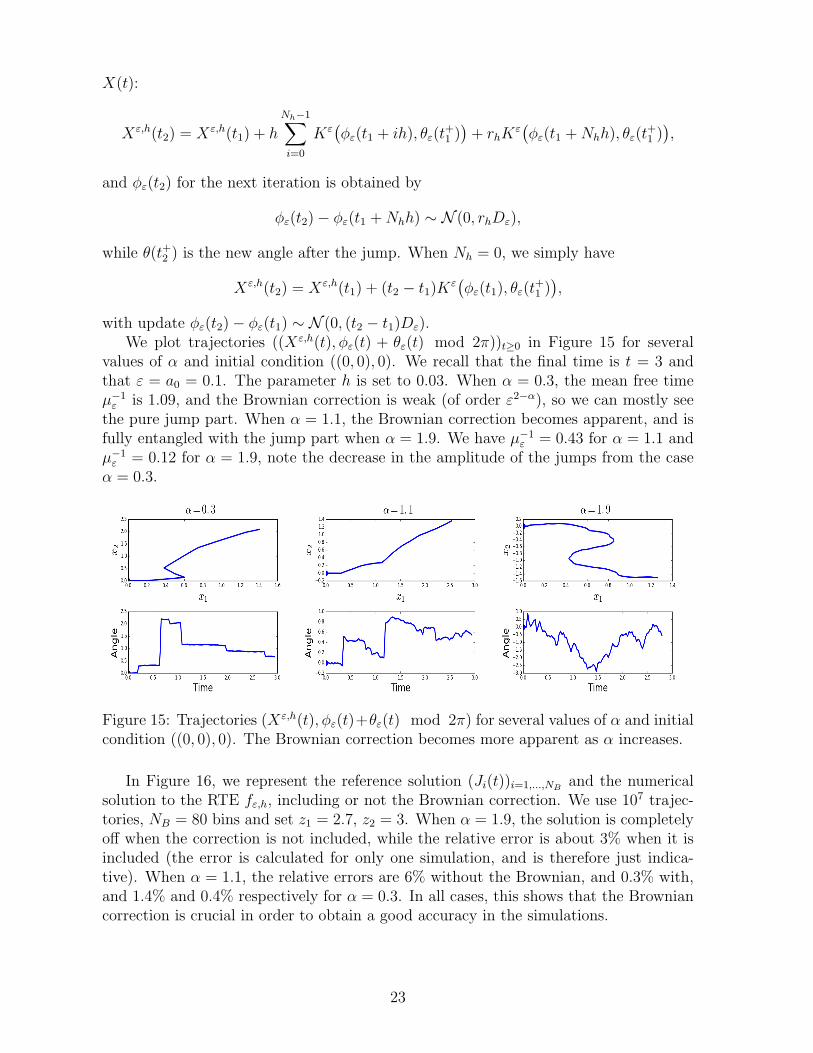
with update φε(t2)− φε(t1) ∼ N (0, (t2 − t1)Dε).We plot trajectories ((Xε,h(t), φε(t) + θε(t) mod 2π))t≥0 in Figure 15 for several
values of α and initial condition ((0, 0), 0). We recall that the final time is t = 3 andthat ε = a0 = 0.1. The parameter h is set to 0.03. When α = 0.3, the mean free timeµ−1ε is 1.09, and the Brownian correction is weak (of order ε2−α), so we can mostly see
the pure jump part. When α = 1.1, the Brownian correction becomes apparent, and isfully entangled with the jump part when α = 1.9. We have µ−1
ε = 0.43 for α = 1.1 andµ−1ε = 0.12 for α = 1.9, note the decrease in the amplitude of the jumps from the caseα = 0.3.
Figure 15: Trajectories (Xε,h(t), φε(t)+θε(t) mod 2π) for several values of α and initialcondition ((0, 0), 0). The Brownian correction becomes more apparent as α increases.
In Figure 16, we represent the reference solution (Ji(t))i=1,...,NB and the numericalsolution to the RTE fε,h, including or not the Brownian correction. We use 107 trajec-tories, NB = 80 bins and set z1 = 2.7, z2 = 3. When α = 1.9, the solution is completelyoff when the correction is not included, while the relative error is about 3% when it isincluded (the error is calculated for only one simulation, and is therefore just indica-tive). When α = 1.1, the relative errors are 6% without the Brownian, and 0.3% with,and 1.4% and 0.4% respectively for α = 0.3. In all cases, this shows that the Browniancorrection is crucial in order to obtain a good accuracy in the simulations.
23

Figure 16: Comparison between the reference solution and the numerical solutions in-cluding or not the Brownian correction. The non corrected solution is completely offwhen α = 1.9, while there is a good accuracy when the Brownian part is included.
5.3 Comparison ACR/AS methods
We compare in this section the performances of the ACR and AS methods. We doso in terms of accuracy versus computational cost for α = 0.7, 1.3, 1.8. We do notaddress smaller values of α since we will see that the ACR method is already muchmore competitive than AS for α = 0.7. We fix a(x) = a0 = 0.1, and use our referencesolution (Ji(t))i=1,...,NB with NB = 20 to quantify the error. As in the previous section,we set t = 3, which is about the characteristic time tS for α = 0.7 and α = 1.3, andabout 2tS for α = 1.8. Since the error is itself a random variable, we average it over 20simulations to obtain a more stable estimate. We then vary the number of particles, thetime stepsize h (see the previous section), and the parameter ε for the ACR method,and record the minimal computational cost required to achieve a given accuracy. Theresults are depicted in Figure 17. The cost is expressed in units of 0.17s, which is thecomputational time to achieve an error of about 10% for a code written in the Julialanguage, and ran in parallel on a 32 cores Intel Xeon E5-2697A at 2.60GHz. Weintegrate the position X(t) in the ACR method as explained in the previous section,while X(t) in the AS case is calculated by a low order quadrature for the integral ofK(t).
In the case α = 0.7, the cost of achieving an error of 0.2% is about 10 times higherfor the AS method. The gap is reduced for lower accuracies, about twice the cost ofAS when the error is 10% for instance. The fact that the ACR method is more efficientis confirmed with α = 1.3 and α = 1.8, with the gap shrinking as α increases. This isexplained on the one hand by the fact that the ACR method is more sensitive to theparameter α than AS since there are more and more collisions as α grows, and on theother that the jumps are smaller for large α which reduces the error in the calculationof X(t) in the AS method. Still, the cost of a 0.5% error when α = 1.8 is more thantwice higher for the AS method. Note that the cost significantly increases when goingfrom an accuracy of about 10% to about 0.1%.
The better performances of the ACR method can be explained as follows: while theprocess (K(t))t≥0 is simulated exactly in the AS method (in the sense that there is noapproximation apart from the collocation sampling), the position X(t) is obtained by
24

Figure 17: Comparison of the AS and ACR methods in terms of cost versus accuracyfor α = 0.7, 1.3, 1.8. The ACR method is consistenly more efficient.
numerical integration of K(t). Since the latter presents rough variations, a sufficientlyfine discretization is needed. A better way to handle the integration of K(t) would to beadapt the stepsize to the random variations of K, which is essentially what is providedby the ACR method: the decomposition of the generator into the pure jump and theBrownian parts allows us to separate the large jumps from the smaller variations. Asa consequence, the former part can be integrated exactly, leading to a reduced errorcompared to the AS method.
5.4 Sensitivity to the parameter ε
The parameter ε is crucial in the ACR method, and it is therefore important to inves-tigate how it is affecting the efficiency. We already know that the mean free time is oforder εα, and that the error is of order ε4−α, which means that there is a trade-off be-tween accuracy and cost in the choice of ε (see Section 2.3). We would like to investigatehere this fact numerically. In Figure 18, left panel, we represent the error as a functionof the number of particles, for α = 0.7, 1.8, and ε = 0.03, 0.1, 0.3 the higher group ofcurves corresponds to α = 1.3. We are in the same setting as the last section, witht = 3, a(x) = 0.1, and a stepsize h = 0.03. We observe as expected that the smaller theε, the smaller the error with a significant margin for α = 0.7, and a much smaller onewhen α = 1.8. This is to be compared with the cost of decreasing ε: in Figure 18, rightpanel, we represent the cost of running a simulation for ε = 0.03, 0.1, 0.3. The referenceis the cost of a simulation with 106 particles, h = 0.03, ε = 0.3 and α = 0.7 (the resultsare qualitatively similar for other choices). When α = 0.7 and α = 1.3, the cost is notvery different when decreasing ε from 0.3 to 0.03, while it increases significantly in thecase α = 1.8 when going from 0.1 and 0.03 (this is explained by the mean free time oforder εα). Since the errors between the cases ε = 0.1 and ε = 0.03 are quite similar asdepicted in the left figure, this suggests that ε = 0.1 is a good compromise and a betterchoice than ε = 0.3 or ε = 0.03.
25

Figure 18: Left: error as a function of the number of particles for various values of α.The upper group of curves corresponds to α = 1.8, and the lower group to α = 0.7.Right: computational cost as a function of ε. Note the significant increases in the caseα = 1.8.
5.5 Comparison Short-Range versus Long-Range underlyingrandom medium
Our goal in this section is to compare the solutions to the RTE (1) with singular kernelsto solutions with integrable kernels. We choose a simple kernel given by a constantfunction, that is
QI(f)(k) = a1
∫S1
(f(p)− f(p))dσ(p).
The process (K(t))t≥0 with generator QI is straightforwardly simulated as it sufficesto draw the angle uniformly over [−π, π]. For a meaningful comparison with singularkernels of the form (2), we choose a1 such that the mean free time associated with QI(namely (2πa1)
−1) is equal to the characteristic time tS associated with the singularkernel. We set as usual a(x) = 0.1, for α = 0.5 and α = 1.8, we display in Figure 19 thesolutions to the RTE on a slab of width 0.2 centered at x2 = 0, as functions of x1, fort = tS, 2tS, 3tS and integrated in angle. We use the initial condition (11). For t = tS,the three solutions for α = 0.5, α = 1.8, and for the constant kernel case (referred as“Uniform” in the figure), are quite similar with the distinction that the scattered part(i.e. the part that lags behind the peak) is weaker in singular cases since scattering ismostly peaked forward. When t = 2tS, significant differences appear, with in particularthe fronts in the singular case being widened by the regularization of the RTE. Thewidening is stronger when α is larger, as expected. On the other hand, the ballisticfront in the uniform case does not change, also as can be expected. When t = 3tS, thefront in the case α = 0.5 merges with the scattered part, while it can still be observedwhen α = 1.8 since forward scattering is stronger.
These results substantiate the claim made in the introduction that inverse problemsbased on transport equations with singular kernels should be more ill-posed than thosewith integrable kernels: inversion strategies are often based on the singularities of thesolution, that here are smoothed out by the RTE.
26

Figure 19: Comparison of solutions in the short-range (red curves) and long-range cases(blue and green curves) at multiples of the characteristic time. Note the regularizationof the front in the long-range case.
We investigate in the next section the effect of the function a of the kernel on theform of the solution.
5.6 Impact of the function a
We use the same setting as in the last section, namely we represent the solutions on aslab around x2 = 0 at multiples of the characteristic time associated with a constantfunction a. We compare the results for a(u) = a0 = 0.1 (with u ≡ k · p), a(u) = a1(u) =(2 + u)/30, and a(u) = a2(u) = 0.1e−(1−u). The coefficients where chosen such thata(1) = a1(1) = a2(1), that is such that the “amplitude” at the singularity is the same inthe three cases. Results are displayed in figure 20. Since the function a2 is more peakedaround u = 1 than a1, which is itself more peaked than a0, its associated scattered partis weaker than in the two other cases.
Figure 20: Comparison of the solutions for constant and non constant functions a.Observe the largest front for the most peaked function.
27

6 Generalizations
We explain in this section how the ACR method can be generalized to collision operatorsof the form
Q(f)(x, k) =
∫S1
f(p)− f(k)
|k − p|1+α(x)a(x, k, p)dσ(p),
which arise for instance when the statistical properties of the underlying random mediavary with the position.
The pure jump part. We start with the generatorQε>. A standard method to handlecompound Poisson processes with parameter-dependent Levy measures is the so-called“fictitious shock method”, see [21], also referred to as “thinning”. The intensity µεdepends now on (x, k), and let
µε := supx∈R2,k∈S1
µε(x, k).
We then generate a compound Poisson process with intensity µε (note that the globalsupremum in the above definition can be localized to yield better efficiency). Supposethe process has a discontinuity at some time t. Then:
• With probability p = 1− µε(X(t), K(t−))/µε, we set K(t+) = K(t−), that is K isnot modified.
• With probability 1− p, K(t−) is modified according to πε(X(t), K(t−), p), where
πε(x, k, p)dσ(p) =a(x, k, p)
π0ε(x, k)|k − p|1+α(x)
dσ(p),
and
π0ε(x, k) =
∫S1
a(x, k, p)
|k − p|1+α(x)dσ(p).
The method is exact, and the question left is how to simulate πε. The rejection methodcan readily be adapted, the constant a being now the supremum of a over (x, k, p). Thestochastic collocation method can also be used in this framework as follows: rewrite a asa(x, k, p) = a(x, k·p, p⊥), where p⊥ = p−(k·p)k, and let A(x, k·p) := supp⊥ a(x, k·p, p⊥).Defining
νε(x, p)dσ(p) =A(x, k · p)
ν0ε |k − p|1+α(x)
dσ(p),
where ν0ε is an appropriate normalization, πε is simulated by rejection sampling with
proposal νε. The distribution νε can then be simulated with the stochastic collocationmethod: discretize the range of the function α into N1 intervals, and that of A into N2
intervals. Consider the resulting N1N2 densities µε,i, i = 1, · · · , N1N2. For each i, onecan generate offline the interpolation polynomial as described in Section 4.2, and storethe coefficients. The accuracy depends on N1N2, but with a polynomial of order 15, wewould just need to store 15N1N2 coefficients, which is not expensive.
28

The Brownian part. Following the calculations of section A.1, the coefficient a(0)in the definition of Dε ≡ Dε(x, k) has to be replaced by a(x, k, k). Assuming there areno jumps between t and t + h, the angle φε can be approximately generated with therelation
φε(t+ h)− φε(t) ∼ N (0, hDε(X(t), K(t))).
If there are jumps in [t, t + h], then the interval is decomposed appropriately, and weapply a formula as above in each subintervals.
7 Conclusion
This work is devoted to Monte Carlo methods for radiative transfer equations with sin-gular collision kernels. We compared the ACR method based on an approximation ofthe generator with the AS method based on the true generator. We showed the superi-ority of the ACR method, due in part to the separation of the large jumps contributionallowing for a more accurate integration of the momentum.
We also compared various methods for the simulation of the jump distribution, andobtained significantly better performances with the stochastic collocation method. Wemade clear of the importance of including the Brownian correction for very singularkernels, and compared solutions to the RTE in the singular case with solutions in theintegrable case. We in particular confirmed the regularization effect of singular kernels.
This work is a first step in the simulation of high frequency wave energy transportin random media with long-range correlations, our ultimate goal being the resolution ofimaging problems with transport-based techniques as in [4, 5]. Various relevant compu-tational issues were not addressed here, in particular how to reduce the variance in thesimulations, and how to adjust the parameter ε to it. A comparison with deterministicmethods is also of importance. Note that these latter methods would need to take aparticular care of the singularity of the kernel. These questions will be the object offuture works, as well as the extension of the Monte Carlo methods to three-dimensionalsettings.
A Appendix
A.1 Proof of Lemma 2.1
Let us start by rewriting the generator as follows
Qε<(g)(θ) =1
21+α
2
∫ICε
a(θ′)(g(θ′ + θ)− g(θ))
(1− cos(θ′))1+α
2
dθ′
=a(0)
21+α
2
∫ICε
g(θ′ + θ)− g(θ)
(1− cos(θ′))1+α
2
dθ′ +1
21+α
2
∫ICε
(a(θ′)− a(0))(g(θ′ + θ)− g(θ))
(1− cos(θ′))1+α
2
dθ′
:= Rε1(θ) +Rε
2(θ),
where ICε = {θ′ ∈ [−π, π], | tan(θ′/4)| ≤ ε/4}.
29
Regarding Rε1, Taylor expanding g up to fourth order, and using symmetries to
cancels the first and third order terms, we find, for some ξθ ∈ (θ, θ + θ′),
Rε1(θ) =
a(0)g′′(θ)
21+α
2+1
∫ICε
θ′2
(1− cos(θ′))1+α
2
dθ′ +a(0)
21+α
2 4!
∫ICε
θ′4g(4)(ξθ)
(1− cos(θ′))1+α
2
dθ′
:= Lεg(θ) +Rε12(θ),
where Lεg is the leading term. Regarding Rε2, we perform again a Taylor expansion on
g up to the fourth order and and using again symmetries, we obtain
Rε2(θ) =
g′′(θ)
21+α
2+1
∫ICε
θ′2(a(θ′)− a(0))
(1− cos(θ′))1+α
2
dθ′ +1
21+α
2 4!
∫ICε
θ′4g(4)(ξθ)(a(θ′)− a(0))
(1− cos(θ′))1+α
2
dθ′.
We use the following lemma in order to treat the terms above.
Lemma A.1 We have∣∣∣∣∣∫ICε
φ2dφ
(1− cos(φ))1+α
2
− 23+α
2
2− αε2−α
∣∣∣∣∣ ≤ 3
23−α
2 (4− α)ε4−α,
and ∫ICε
φ4
(1− cos(φ))1+α
2
dφ ≤ 25+α
2
4− αε4−α.
As a result, Taylor expanding a up to the second order and using symmetries to cancelthe first order term, we have for any θ ∈ [π, π],∣∣∣∣Qε<(g)(θ)− a(0)ε2−α
2− αg′′(θ)
∣∣∣∣ ≤ ε4−α
4− α
(‖a‖∞ + ‖a′′‖∞
)(‖g′′‖∞ + ‖g(4)‖∞
).
Proof. [of Lemma A.1] Using that
1− cos(θ′) = 2 sin2(θ′/2) =4 tan2(θ′/4)
(1 + tan2(θ′/4))2,
we have, with the change of variable u = tan(φ/4),∫ICε
φ2dφ
(1− cos(φ))1+α
2
=1
23 1+α2
∫ICε
φ2(1 + tan2(φ/4))1+αdφ
| tan(φ/4)|1+α
=26
23 1+α2
∫ ε/4
−ε/4
arctan2(u)(1 + u2)αdu
|u|1+α.
Now, using standard analysis, we find∣∣∣∣∣∫ ε/4
−ε/4
arctan2(u)(1 + u2)αdu
|u|1+α−∫ ε/4
−ε/4
|u|2du|u|1+α
∣∣∣∣∣ ≤ 6
∫ ε/4
−ε/4
|u|4du|u|1+α
,
with ∫ ε/4
0
u3−αdu =ε4−α
28−2α(4− α)and
∫ ε/4
0
u1−αdu =ε2−α
24−2α(2− α).
30

Gathering all previous estimates, we obtain∣∣∣∣∣∫ICε
φ2dφ
(1− cos(φ))1+α
2
− 23+α
2
2− αε2−α
∣∣∣∣∣ ≤ 3
23−α
2 (4− α)ε4−α,
concluding the proof of the first point. The second point of the lemma follows from thesame lines as above, and we have∫
ICε
φ4dφ
(1− cos(φ))1+α
2
=210
23 1+α2
∫ ε
−ε
arctan4(u)(1 + u2)αdu
u1+α
≤ 25+α
2
4− αε4−α.
A.2 Proof of Proposition 2.2
Let uε = f ε − f , which we assume is smooth in order to justify the formal calculations.With the notation of Lemma 2.1, uε satisfies
∂tuε + k · ∇xu
ε = Qε>uε +Dε
2∂2θu
ε −Rε[f ], uε(t = 0) = 0. (13)
For (·, ·) the scalar product on R2 × S1, we have
(Qε>uε, uε) ≤ 0, (∂2φu
ε, uε) ≤ 0,
and therefore, we obtain from (13),
1
2
d
dt‖uε(t)‖2L2(R+×S1) ≤ (Rε[f(t)], uε(t)).
This yields from the Cauchy-Schwarz inequality,
d
dt‖uε(t)‖L2(R+×S1) ≤ ‖Rε[f(t)]‖L2(R2×S1),
and the conclusion follows from Lemma 2.1.
A.3 Proof of Lemma 4.1
Let us assume that Θ is a random variable with density πε, and let g be a boundedcontinuous function. With the notation of section 2.2, we have
E[g(Θ)] =
∫Iε,+
g(θ)a(θ)
Π0ε,+(1− cos(θ))(1+α)/2
dθ
=1
2(1+α)/2Π0ε,+
∫Iε,+
g(θ)a(θ)
sin1+α(θ/2)dθ
31

and making the change of variable θ → 2θ,
E[g(Θ)] =2
2(1+α)/2Π0ε,+
∫I′ε,+
g(2θ)a(2θ)
sin1+α(θ)dθ,
withI ′ε,+ := {θ ∈ (0, π/2) s.t. tan(θ/2) > ε/4}.
Now, using that sin(θ) = 2 tan(θ/2)/(1 + tan2(θ/2)), and making again the change ofvariable θ → 2θ, we obtain
E[g(Θ)] =2
23(1+α)/2Π0ε,+
∫I′ε,+
g(2θ)a(2θ)
tan1+α(θ/2)(1 + tan2(θ/2))1+αdθ
=22
23(1+α)/2Π0ε,+
∫I′′ε,+
g(4θ)a(4θ)
tan1+α(θ)(1 + tan2(θ))1+αdθ,
withI ′′ε,+ := {θ ∈ (0, π/4) s.t. tan(θ) > ε/4}.
Now, with v = tan(θ), we finally obtain
E[g(Θ)] =1
2(3α−1)/2Π0ε,+
∫g(4 arctan(v))
a(4 arctan(v))(1 + v2)α
v1+α1(ε/4,1)(v)dv
= E[g(4 arctan(V ))],
which concludes the proof.
A.4 Gauss and Gauss-Lobatto quadratures
Gauss quadrature. This is classical material, and the standard method is the Golub-Welsch algorithm [11]. For a measure µ(x), and given a three-term recurrence relationbetween orthogonal polynomials Pk for the measure µ of the form
Pk+1(x) = (x− αk)Pk(x)− βkPk−1, k ≥ 0, P−1(x) = 0, P0(x) = 1,
one forms the N × N symmetric tridiagonal matrix J with diagonal (α0, · · · , αN−1)and upper diagonal (
√β1, · · · ,
√βN−2). The collocation nodes of the N nodes Gauss
quadrature are then the eigenvalues of J . The important point is therefore to obtain thecoefficient αk and βk. There is simple method based on the moments of µ, which unfor-tunately becomes numerically unstable when about more than 10 collocations points areneeded. We then use a different approach based on a discretization method explicitedin [9]. The idea is to discretize the measure µ as
µ(x) =P∑p=1
wpδ(x− xp),
for some weights wp and points xp to be determined. We then obtain a three-termrecurrence relation with coefficients (αPk , β
Pk ) for this discrete measure using the Stieljes
32

algorithm (see again [9]), where the limit of (αPk , βPk ) as P → ∞ yields the coefficients
of the original measure µ. The choice of wp and xp is important for the efficiency ofthe method, and is done as follows: for some weight function ω(x) for which Gaussquadrature nodes yp and weights γp can be easily calculated, we write (with an abuseof notation, we suppose µ has density µ(x)), for some interval I,∫
I
f(x)µ(x)dx =
∫I
f(x)µ(x)
ω(x)ω(x)dx '
P∑p=1
f(yp)µ(yp)
ω(yp)γp.
We then set xp = yp, and wp = µ(xp)γp/ω(xp). As an example, consider the collocation
method of Section 4.2. We have µ(x) = q1(x) for x ∈ [0, 1 − ε2
4], and we choose
ω(x) = (1 − x)δ−1, for δ = 0.1, which is a Gauss-Jacobi type weight. This choice ismade since, as the function p1, ω has a singularity at x = 1. The associated nodesand weights are known and tabulated, generally over the interval [−1, 1]. We then doa linear transformation to relocate them to the interval [0, 1 − ε2
4]. The overall cost of
the calculation of the collocation points is negligible compared to complete simulationof the RTE.
Gauss-Lobatto quadrature. The procedure is direct using what is above. If I =[a, b], then define the measure ν(x) = (x − a)(b − x)µ(x). The interior nodes of theGauss-Lobatto rule for µ are then the Gauss nodes for ν, see [8].
A.5 Semi-analytical solution
We derive here a representation formula for a particular solution to (1). For f thesolution to (1) with an initial condition of the form (11) and x = (x1, x2), let
g(t, x1, k) =
∫Rf(t, (x1, x2), k)dx2, k ∈ S1.
Writing k = (cos θ, sin θ) and z = x1 for convenience, g solves (assuming f decayssufficiently fast at the infinity),
∂tg + cos θ∂zg = Q(g) = a0
∫S1
g(p)− g(k)
|k − p|1+αdσ(p).
We decompose then g into Fourier modes as
g(t, z, θ) =∑`≥0
g`(t, z)e`(θ), with e0 =1√2π, e` =
cos `θ√π, ` ≥ 1.
Denoting by λ` the eigenvalues of the operator Q explicitely defined in (7), we find thesystem of equations
∂tg0 + 1√2∂zg1 = λ0g0
∂tg1 + 1√2∂zg0 + 1
2∂zg2 = λ1g1
∂tg` + 12∂zg`−1 + 1
2∂zg`+1 = λ`g`, ` ≥ 2.
33

After taking the Fourier transform in z, we find
∂tg`(t, ξ) = λ`g` − iξ(c`g`+1 + d`g`−1) (14)
where
c0 =1√2, d0 = 0, d1 =
1√2, c` =
1
2, ` ≥ 1, d` =
1
2, ` ≥ 2.
Storing the coefficient g` up to some order ` = L into a vector gL, (14) can be writteninto the matrix form
∂tgL(t, ξ) = AL(ξ)gL(t, ξ).
This gives us an approximation gL of g represented by
gL(t, z, θ) =1
2π
L∑`=0
(∫ReizξetAL(ξ)gL(0, ξ)dξ
)`
e`(θ),
where (f)` is the component of f along e`. If f0 in (11) is the initial condition, theng(t = 0) reads
g(0, z, θ) =1√
2πc2e−
z2
2c21
2π(1 + cos θ) =
1√2πc2
e−z2
2c2
(e0√2π
+e1√4π
),
which admits as Fourier transform
g(0, ξ, θ) = e−c2ξ2/2
(e0√2π
+e1√4π
).
The function Ji defined by (12) is then finally
Ji(t) =
∫ z2
z1
∫ θi+1
θi
g(t, z, θ)dzdθ =1
2π
L∑`=0
(∫R
eiz2ξ − eiz1ξ
iξetAL(ξ)g(0, ξ)dξ
)`
∫ θi+1
θi
e`(θ)dθ,
which we evaluate numerically.
References
[1] S. Asmussen and J. Rosiski, Approximations of small jumps of lvy processes with a view towardssimulation, J. Appl. Probab., 38 (2001), pp. 482–493.
[2] K. B. Athreya, D. McDonald, and P. Ney, Limit theorems for semi-markov processes andrenewal theory for markov chains, Ann. Probab., 6 (1978), pp. 788–797.
[3] G. Bal, Inverse transport theory and applications, Inverse Problems, 25 (2009).
[4] G. Bal and O. Pinaud, Imaging using transport models for wave-wave correlations, M3AS, 21(5)(2011), pp. 1071–1093.
[5] G. Bal and K. Ren, Transport-based imaging in random media, SIAM Applied Math., 68(6)(2008), pp. 1738–1762.
[6] S. Cohen and J. Rosinski, Gaussian approximation of multivariate lvy processes with applica-tions to simulation of tempered stable processes, Bernoulli, 13 (2007), pp. 195–210.
34

[7] S. Dolan, C. Bean, and R. B., The broad-band fractal nature of heterogeneity in the uppercrust from petrophysical logs, Geophys. J. Int., 132 (1998), pp. 489–507.
[8] W. Gautschi, Orthogonal polynomials: computation and approximation, Numerical Mathematicsand Scientific Computation, Oxford University Press, New York, 2004. Oxford Science Publica-tions.
[9] W. Gautschi, Orthogonal polynomials (in matlab), Journal of Computational and Applied Math-ematics, 178 (2005), pp. 215 – 234. Proceedings of the Seventh International Symposium onOrthogonal Polynomials,Special Functions and Applications.
[10] F. Golse, P.-L. Lions, B. Perthame, and R. Sentis, Regularity of the moments of thesolution of a transport equation, Journal of Functional Analysis 76, (1988), pp. 110–125.
[11] G. H. Golub and J. H. Welsch, Calculation of gauss quadrature rules, Mathematics of Com-putation, 23 (1969), pp. 221–s10.
[12] C. Gomez, Radiative transport limit for the random Schrodinger equation with long-range corre-lations, J. Math. Pures Appl. (9), 98 (2012), pp. 295–327.
[13] C. Gomez, O. Pinaud, and L. Ryzhik, Radiative transfer with long-range interactions: regu-larity and asymptotics, to appear in SIAM MMS.
[14] , Hypoelliptic estimates in radiative transfer, CPDE, 1 (2016), pp. 150–184.
[15] L. A. Grzelak, J. Witteveen, M. Suarez-Taboada, and C. W. Oosterlee, The stochasticcollocation monte carlo sampler: Highly efficient sampling from’expensive’distributions, Availableat SSRN: https://ssrn.com/abstract=2529691 or http://dx.doi.org/10.2139/ssrn.2529691, (2015).
[16] A. Haghighat, Monte Carlo Methods for Particle Transport, CRC Press, 2014.
[17] W. K. Hastings, Monte carlo sampling methods using markov chains and their applications,Biometrika, 57 (1970), pp. 97–109.
[18] S. Holm and R. Sinkus, A unifying fractional wave equation for compressional and shear wave,J. Acoust. Soc. Am., 1 (2010), pp. 542–548.
[19] A. Ishimaru, Wave Propagation and Scattering in Random Media, New York: Academics, 1978.
[20] A. D. Kim and J. B. Keller, Light propagation in biological tissue, J. Opt. Soc. Am. A, 20(2003), pp. 92–98.
[21] B. Lapeyre, E. Pardoux, and R. Sentis, Introduction to Monte Carlo Methods for Transportand Diffusion Equations, Oxford, 1998.
[22] E. W. Larsen and J. B. Keller, Asymptotic solution of neutron transport problems for smallmean free paths, J. Math. Phys., 15 (1974), pp. 75–81.
[23] C. Leakeas and E. Larsen, Generalized Fokker-Planck approximations of particle transportwith highly forward-peaked scattering, Nuclear science and engineering, 137 (2001), pp. 236–250.
[24] N. Metropolis, A. W. Rosenbluth, M. N. Rosenbluth, A. H. Teller, and E. Teller,Equation of state calculations by fast computing machines, The Journal of Chemical Physics, 21(1953), pp. 1087–1092.
[25] G. Pomraning, The fokker-planck operator as an asymptotic limit, Mathematical Models andMethods in Applied Sciences, 02 (1992), pp. 21–36.
[26] C. Rao, W. Jiang, and N. Ling, Spatial and temporal characterization of phase fluctuations innon-kolmogorov atmospheric turbulence, Journal of Modern Optics, 47 (2000), pp. 1111–1126.
[27] F. Roddier, The effects of atmospheric turbulence in optical astronomy, Progress in optics. Vol-ume 19. Amsterdam, North-Holland Publishing Co., 19 (1981), pp. 281–376.
[28] L. Ryzhik, G. Papanicolaou, and J. B. Keller, Transport equations for elastic and otherwaves in random media, Wave Motion, 24 (1996), pp. 327–370.
35

[29] S. Samko, On inversion of fractional spherical potentials by spherical hypersingular operators, inSingular integral operators, factorization and applications, vol. 142 of Oper. Theory Adv. Appl.,Birkhauser, Basel, 2003, pp. 357–368.
[30] G. Samorodnitsky and T. M.S., Stable Non-Gaussian Processes, CRC Press, 1994.
[31] P. Sheng, Introduction to Wave Scattering, Localization and Mesoscopic Phenomena, AcademicPress, New York, 1995.
[32] C. Sidi and F. Dalaudier, Turbulence in the stratified atmosphere: Recent theoretical devel-opments and experimental results, Adv. in Space Res., 10 (1990), pp. 25–36.
[33] J. Spanier and E. M. Gelbard, Monte Carlo principles and neutron transport problems,Addison-Wesley, Reading, Mass., 1969.
[34] T. M. Srensen and F. E. Benth, Levy process simulation by stochastic step functions, SIAMJournal on Scientific Computing, 35 (2013), pp. A2207–A2224.
[35] R. Weron, On the chambers-mallows-stuck method for simulating skewed stable random variables,Statistics and Probability Letters, 28 (1996), pp. 165 – 171.
36