a 3d radiative transfer solver for atmospheric heating ... · history of radiative transfer...
TRANSCRIPT

A 3D Radiative Transfer Solver for Atmospheric
Heating Rates – powered by PETSc
Fabian Jakub
LMU - Meteorological Institute Munich
June 16, 2015
1 / 22
Radiative Transfer in atmospheric models
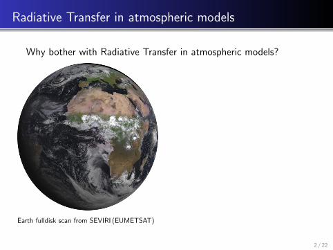
Why bother with Radiative Transfer in atmospheric models?
Earth fulldisk scan from SEVIRI (EUMETSAT)
I Sun heats surface and
atmosphere
I Earth emits to space
I Radiation ultimately drives
flow
.. on large scales
.. and on small scales
2 / 22
Radiative Transfer in atmospheric models
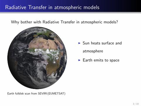
Why bother with Radiative Transfer in atmospheric models?
Earth fulldisk scan from SEVIRI (EUMETSAT)
I Sun heats surface and
atmosphere
I Earth emits to space
I Radiation ultimately drives
flow
.. on large scales
.. and on small scales
2 / 22
Radiative Transfer in atmospheric models
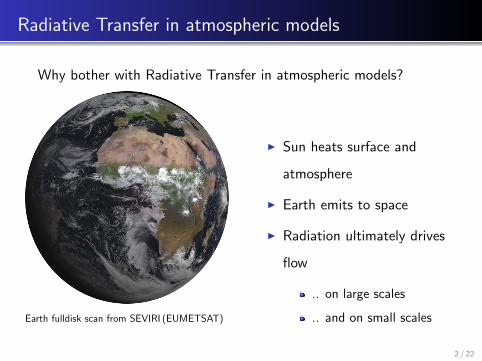
Why bother with Radiative Transfer in atmospheric models?
Earth fulldisk scan from SEVIRI (EUMETSAT)
I Sun heats surface and
atmosphere
I Earth emits to space
I Radiation ultimately drives
flow
.. on large scales
.. and on small scales
2 / 22
History of Radiative Transfer
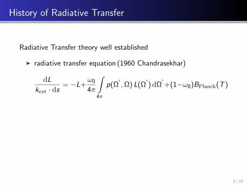
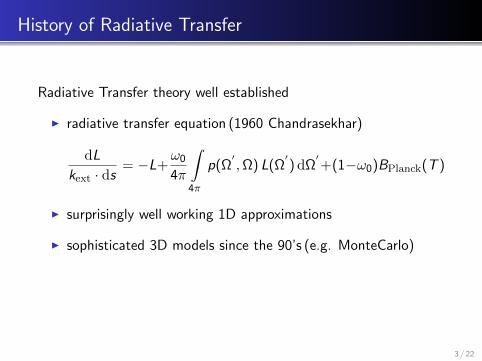
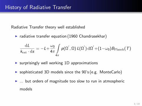
Radiative Transfer theory well established
I radiative transfer equation (1960 Chandrasekhar)
dL
kext · ds= −L+
ω0
4π
∫4π
p(Ω′,Ω) L(Ω
′)dΩ
′+(1−ω0)BPlanck(T )
I surprisingly well working 1D approximations
I sophisticated 3D models since the 90’s (e.g. MonteCarlo)
I ... but orders of magnitude too slow to run in atmospheric
models
3 / 22
History of Radiative Transfer
Radiative Transfer theory well established
I radiative transfer equation (1960 Chandrasekhar)
dL
kext · ds= −L+
ω0
4π
∫4π
p(Ω′,Ω) L(Ω
′)dΩ
′+(1−ω0)BPlanck(T )
I surprisingly well working 1D approximations
I sophisticated 3D models since the 90’s (e.g. MonteCarlo)
I ... but orders of magnitude too slow to run in atmospheric
models
3 / 22
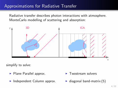
Approximations for Radiative Transfer
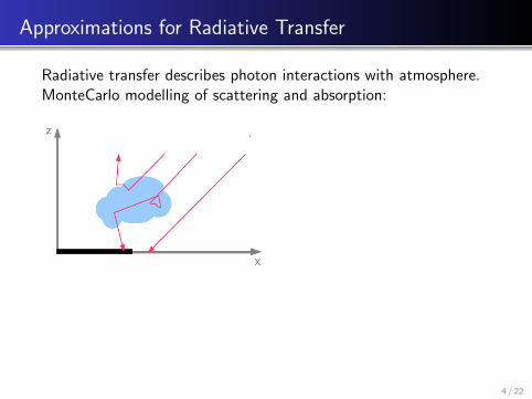
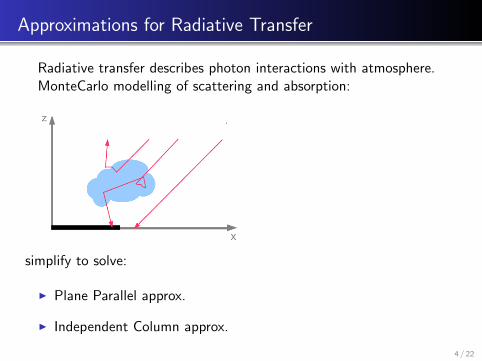
Radiative transfer describes photon interactions with atmosphere.MonteCarlo modelling of scattering and absorption:
simplify to solve:
I Plane Parallel approx.
I Independent Column approx.
I Twostream solvers
I diagonal band-matrix (5)
4 / 22
Approximations for Radiative Transfer
Radiative transfer describes photon interactions with atmosphere.MonteCarlo modelling of scattering and absorption:
simplify to solve:
I Plane Parallel approx.
I Independent Column approx.
I Twostream solvers
I diagonal band-matrix (5)
4 / 22
Approximations for Radiative Transfer
Radiative transfer describes photon interactions with atmosphere.MonteCarlo modelling of scattering and absorption:
simplify to solve:
I Plane Parallel approx.
I Independent Column approx.
I Twostream solvers
I diagonal band-matrix (5)
4 / 22

Why care for 3D radiation now? – a matter of resolution
Complex cloud radiation interaction
Visualization done with libRadtran.org/MYSTIC (Monte carlo code for the phYSically correct Tracing of photons In Cloudy atmospheres)
Mayer, B., 2009. Radiative transfer in the cloudy atmosphere (EPJ Web of Conferences)
5 / 22
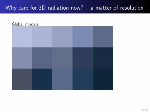
Why care for 3D radiation now? – a matter of resolution
Global models
Visualization done with libRadtran.org/MYSTIC (Monte carlo code for the phYSically correct Tracing of photons In Cloudy atmospheres)
Mayer, B., 2009. Radiative transfer in the cloudy atmosphere (EPJ Web of Conferences)
5 / 22
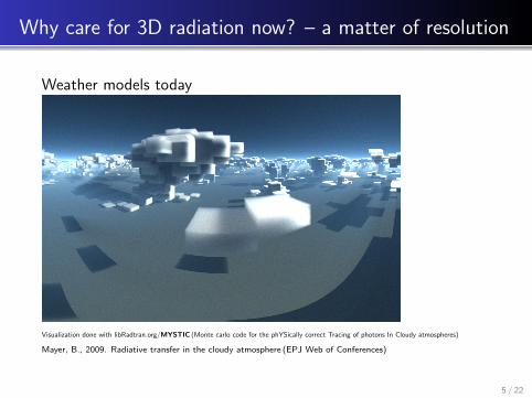
Why care for 3D radiation now? – a matter of resolution
Weather models today
Visualization done with libRadtran.org/MYSTIC (Monte carlo code for the phYSically correct Tracing of photons In Cloudy atmospheres)
Mayer, B., 2009. Radiative transfer in the cloudy atmosphere (EPJ Web of Conferences)
5 / 22
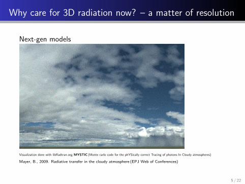
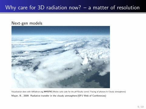
Why care for 3D radiation now? – a matter of resolution
Next-gen models
Visualization done with libRadtran.org/MYSTIC (Monte carlo code for the phYSically correct Tracing of photons In Cloudy atmospheres)
Mayer, B., 2009. Radiative transfer in the cloudy atmosphere (EPJ Web of Conferences)
5 / 22
Why care for 3D radiation now? – a matter of resolution
Next-gen models
Visualization done with libRadtran.org/MYSTIC (Monte carlo code for the phYSically correct Tracing of photons In Cloudy atmospheres)
Mayer, B., 2009. Radiative transfer in the cloudy atmosphere (EPJ Web of Conferences)
5 / 22
Does 3D Radiative Transfer impact cloud evolution?
3D radiative transfer may affect
I cloud evolution and lifetime
I microphysical processes (condensation, nucleation)
I precipitation onset/amount
I convective organization
Can we answer this by high resolution modelling?
6 / 22
Does 3D Radiative Transfer impact cloud evolution?
3D radiative transfer may affect
I cloud evolution and lifetime
I microphysical processes (condensation, nucleation)
I precipitation onset/amount
I convective organization
Can we answer this by high resolution modelling?
6 / 22
HD(CP)2 project (www.hdcp2.eu)
I run hindcasts over Central Europe
I 100m horizontal resolution
I grids consisting of 10.000 x 15.000 x 300 voxels
I first develop a model capable of running it (ICON)
I . . . with the goal to develop improved parametrizations for
weather and climate predictions
7 / 22

The Tenstream solver
A new concept for a solver – what do we want?
I3RC cloud scene, benchmark heating rate
calculation with MYSTIC (MonteCarlo code)
I accurately approximate 3D
effects
I has to be several orders of
magnitude faster than state
of the art 3D solvers
I parallelizable on modern
machines
8 / 22
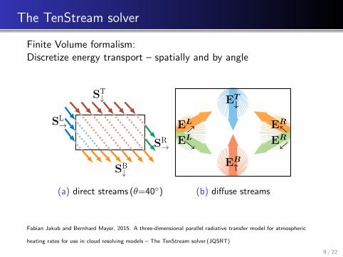
The TenStream solver
Finite Volume formalism:Discretize energy transport – spatially and by angle
ST↓
SL→
SR→
SB↓
(a) direct streams (θ=40)
EB↑
ET↓
ERւEL
ց
ERտEL
ր
(b) diffuse streams
Fabian Jakub and Bernhard Mayer, 2015. A three-dimensional parallel radiative transfer model for atmospheric
heating rates for use in cloud resolving models – The TenStream solver (JQSRT)
9 / 22
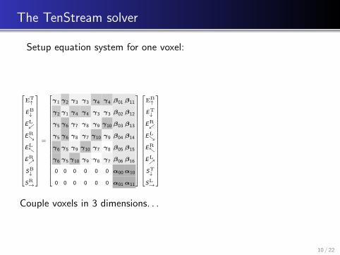
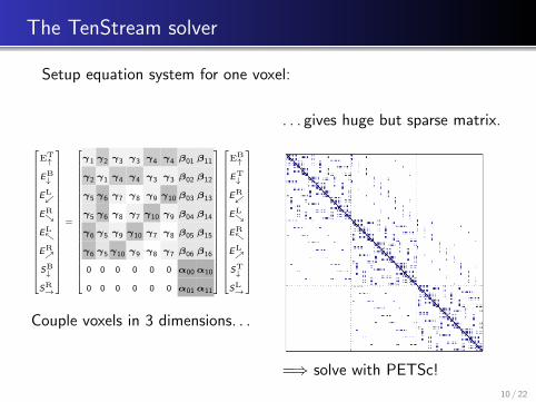
The TenStream solver
Setup equation system for one voxel:
ET↑
EB↓
EL
ER
EL
ER
SB↓
SR→
=
γ1 γ2 γ3 γ3 γ4 γ4 β01 β11
γ2 γ1 γ4 γ4 γ3 γ3 β02 β12
γ5 γ6 γ7 γ8 γ9 γ10 β03 β13
γ5 γ6 γ8 γ7 γ10 γ9 β04 β14
γ6 γ5 γ9 γ10 γ7 γ8 β05 β15
γ6 γ5 γ10 γ9 γ8 γ7 β06 β16
0 0 0 0 0 0 α00 α10
0 0 0 0 0 0 α01 α11
EB↑
ET↓
ER
EL
ER
EL
ST↓
SL→
Couple voxels in 3 dimensions. . .
. . . gives huge but sparse matrix.
=⇒ solve with PETSc!
10 / 22
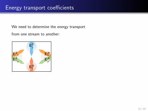
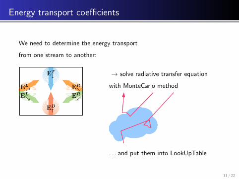
Energy transport coefficients
We need to determine the energy transport
from one stream to another:
EB↑
ET↓
ERւEL
ց
ERտEL
ր
→ solve radiative transfer equation
with MonteCarlo method
. . . and put them into LookUpTable
11 / 22
Energy transport coefficients
We need to determine the energy transport
from one stream to another:
EB↑
ET↓
ERւEL
ց
ERտEL
ր
→ solve radiative transfer equation
with MonteCarlo method
. . . and put them into LookUpTable
11 / 22
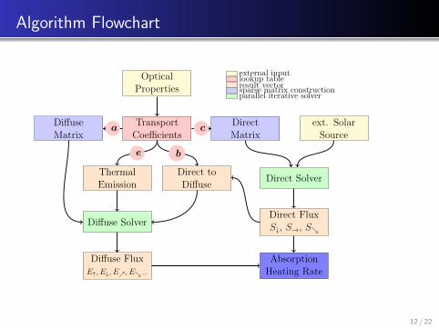
Algorithm Flowchart
OpticalProperties
TransportCoefficients
DirectMatrix
ext. SolarSource
Direct Solver
Direct FluxS↓, S→, Sց
Direct toDiffuse
ThermalEmission
DiffuseMatrix
Diffuse Solver
Diffuse FluxE↑, E↓, Eր, Eց ···
AbsorptionHeating Rate
be
a c
external inputlookup tableresult vectorsparse matrix constructionparallel iterative solver
12 / 22
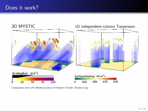
Does it work?
3D MYSTIC 1D independent-column Twostream
Computations done with libRadtran (Library for Radiative Transfer, libradtran.org)
13 / 22
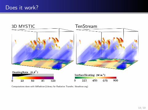
Does it work?
3D MYSTIC TenStream
Computations done with libRadtran (Library for Radiative Transfer, libradtran.org)
13 / 22
Couple Tenstream to atmospheric model
We coupled the TenStream solver to the UCLA - Large EddySimulation (LES)
I LES model atmospheric flow with resolutions from 10m to
1km
I includes dynamics, turbulence, microphysics and radiation
I TenStream solver factor 5-10 more expensive compared to 1D
solver
14 / 22

Impact on convective organization
Simulate 30 km× 30 km domain with different radiative transfer
1D
3D
15 / 22
Current state and a glimpse at whats to come..
Conclusions
I Rapid development of parallel solver with PETSc
I Solve rad. transfer eq. in voxel with MonteCarlo methods
I Successfull integration in LES model
Outlook
I Determine 3D-radiation ↔ cloud interaction
I Implement in icosahedral model ICON
I Make algorithm ready for large scale computations –
HD(CP)2-Project
16 / 22
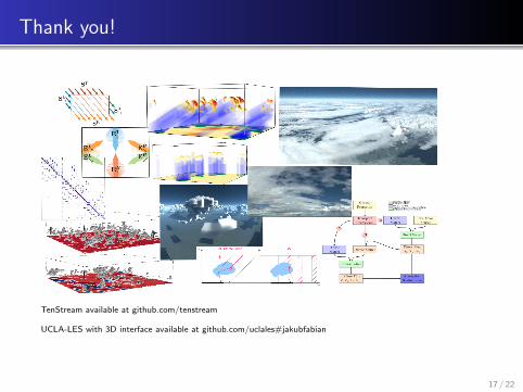
Thank you!
TenStream available at github.com/tenstream
UCLA-LES with 3D interface available at github.com/uclales#jakubfabian
17 / 22
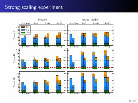
Strong scaling experiment
1
3
5
7
9
11
Nco
res1
ILU
1
MG
5θ=None
ILU
1IL
U1
MG
5M
G5
θ=0
ILU
1IL
U1
MG
5M
G5
θ=60
ILU
1IL
U1
MG
5M
G5
θ=78
clearsky
Edir
Ediff
coeff
ILU
1
MG
5
θ=None
ILU
1IL
U1
MG
5M
G5
θ=0
ILU
1IL
U1
MG
5M
G5
θ=60
ILU
1IL
U1
MG
5M
G5
θ=78
warm−bubble
1
3
5
7
9
11
Nco
res32
ILU
1
MG
5
θ=None
ILU
1IL
U1
MG
5M
G5
θ=0IL
U1
ILU
1
MG
5M
G5θ=60
ILU
1IL
U1
MG
5M
G5
θ=78
ILU
1
MG
5
θ=None
ILU
1IL
U1
MG
5M
G5
θ=0
ILU
1IL
U1
MG
5M
G5
θ=60
ILU
1IL
U1
MG
5M
G5
θ=78
1
3
5
7
9
11
Nco
res12
8
ILU
1
MG
5
θ=None
ILU
1IL
U1
MG
5M
G5
θ=0
ILU
1IL
U1
MG
5M
G5
θ=60
ILU
1IL
U1
MG
5M
G5
θ=78
ILU
1
MG
5
θ=None
ILU
1IL
U1
MG
5M
G5
θ=0IL
U1
ILU
1
MG
5M
G5
θ=60
ILU
1IL
U1
MG
5M
G5
θ=78
18 / 22
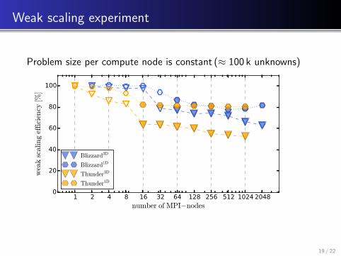
Weak scaling experiment
Problem size per compute node is constant (≈ 100 k unknowns)
1 2 4 8 16 32 64 128 256 512 1024 2048number of MPI−nodes
0
20
40
60
80
100
wea
ksc
alin
gef
fici
ency
[%]
Blizzard3D
Blizzard1D
Thunder3D
Thunder1D
19 / 22
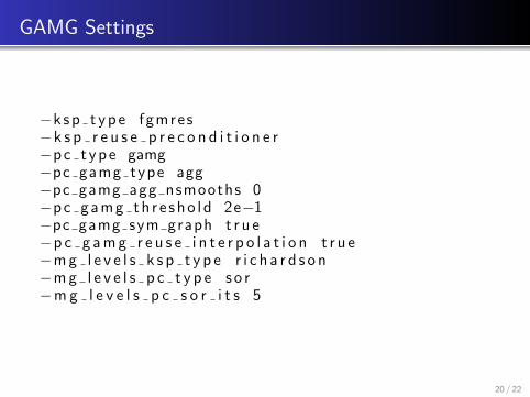
GAMG Settings
−k s p t y p e fgmres−k s p r e u s e p r e c o n d i t i o n e r−p c t y p e gamg−pc gamg type agg−pc gamg agg nsmooths 0−p c g a m g t h r e s h o l d 2e−1−pc gamg sym graph t r u e−p c g a m g r e u s e i n t e r p o l a t i o n t r u e−m g l e v e l s k s p t y p e r i c h a r d s o n−m g l e v e l s p c t y p e s o r−m g l e v e l s p c s o r i t s 5
20 / 22
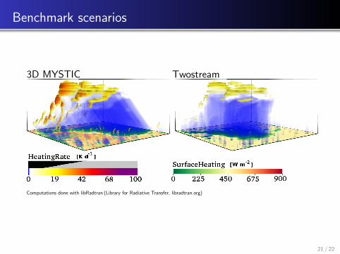
Benchmark scenarios
3D MYSTIC Twostream
Computations done with libRadtran (Library for Radiative Transfer, libradtran.org)
21 / 22
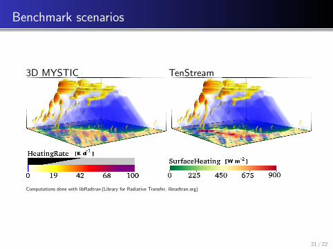
Benchmark scenarios
3D MYSTIC TenStream
Computations done with libRadtran (Library for Radiative Transfer, libradtran.org)
21 / 22
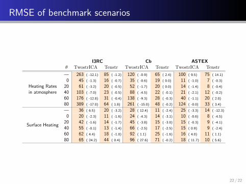
RMSE of benchmark scenarios
I3RC Cb ASTEXθ TwostrICA Tenstr TwostrICA Tenstr TwostrICA Tenstr
Heating Ratesin atmosphere
— 263 ( -12.1) 85 ( -1.2) 120 ( -0.9) 65 ( 2.4) 100 ( 9.5) 75 ( 14.1)
0 45 ( -1.3) 16 ( -0.7) 35 ( -0.6) 19 ( 0.0) 11 ( -1.0) 7 ( -0.3)
20 61 ( -3.2) 20 ( -0.5) 52 ( -1.7) 20 ( 0.0) 14 ( -1.4) 8 ( -0.4)
40 103 ( -7.0) 23 ( -0.5) 88 ( -4.5) 22 ( -0.1) 21 ( -2.1) 12 ( -0.2)
60 176 ( -12.8) 31 ( -0.4) 138 ( -9.3) 28 ( -0.3) 40 ( -1.1) 20 ( 2.0)
80 389 ( -17.0) 64 ( 1.8) 261 ( -15.0) 48 ( -0.2) 124 ( -0.0) 33 ( 3.4)
Surface Heating
— 36 ( 6.5) 20 ( -3.2) 28 ( 12.4) 11 ( -2.4) 25 ( -3.3) 14 ( -12.3)
0 20 ( -2.3) 11 ( -1.6) 24 ( -4.3) 14 ( -3.1) 10 ( -0.6) 8 ( -4.5)
20 42 ( -1.6) 14 ( -1.7) 45 ( -3.8) 15 ( -3.0) 15 ( -0.3) 9 ( -4.1)
40 55 ( -0.1) 13 ( -1.4) 66 ( -2.5) 17 ( -2.5) 15 ( 0.9) 9 ( -2.4)
60 62 ( 4.4) 18 ( -1.0) 92 ( 1.1) 25 ( -1.6) 16 ( 4.0) 11 ( 1.1)
80 65 ( 24.2) 44 ( 0.4) 96 ( 27.6) 71 ( -0.2) 18 ( 11.7) 10 ( 5.6)
22 / 22