monte carlo solution of a radiative heat transfer...

MONTE CARLO SOLUTION OF A RADIATIVE HEAT TRANSFER PROBLEM IN A 3-D RECTANGULAR ENCLOSURE CONTAINING ABSORBING,

EMITTING, AND ANISOTROPICALLY SCATTERING MEDIUM

A THESIS SUBMITTED TO THE GRADUATE SCHOOL OF NATURAL AND APPLIED SCIENCES

OF THE MIDDLE EAST TECHNICAL UNIVERSITY

BY

GÖKMEN DEMİRKAYA

IN PARTIAL FULFILLMENT OF THE REQUIREMENTS FOR THE DEGREE OF

MASTER OF SCIENCE IN

THE DEPARTMENT OF MECHANICAL ENGINEERING

DECEMBER 2003

Approval of the Graduate School of Natural and Applied Science

_____________________

Prof. Dr. Canan Özgen

Director

I certify that this thesis satisfies all the requirements as a thesis for the

degree of Master of Science

___________________ Prof. Dr. Kemal İder

Head of Department

This is to certify that we have read this thesis and that in our opinion it is

fully adequate, in scope and quality, as a thesis for the degree of Master of

Science.

___________________ Prof. Faruk Arınç

Supervisor

Examining Committee Members

Prof. Dr. Ediz Paykoç (Chairperson) ___________________

Prof. Dr. Faruk Arınç (Supervisor) ___________________

Prof. Dr. Nevin Selçuk ___________________

Asst. Prof. Dr. İlker Tarı ___________________

Prof. Dr. Zafer Dursunkaya ___________________

ABSTRACT

MONTE CARLO SOLUTION OF A RADIATIVE HEAT TRANSFER

PROBLEM IN A 3-D RECTANGULAR ENCLOSURE CONTAINING

ABSORBING, EMITTING, AND ANISOTROPICALLY SCATTERING

MEDIUM

Demirkaya, Gökmen

M.Sc., Deparment of Mechanical Engineering

Supervisor: Prof. Dr. Faruk Arınç

December 2003, 87 pages

In this study, the application of a Monte Carlo method (MCM) for

radiative heat transfer in three-dimensional rectangular enclosures was

investigated. The study covers the development of the method from simple

surface exchange problems to enclosure problems containing absorbing,

emitting and isotropically/anisotropically scattering medium.

The accuracy of the MCM was first evaluated by applying the

method to cubical enclosure problems. The first one of the cubical enclosure

problems was prediction of radiative heat flux vector in a cubical enclosure

containing purely, isotropically and anisotropically scattering medium with

non-symmetric boundary conditions. Then, the prediction of radiative heat

flux vector in an enclosure containing absorbing, emitting, isotropically and

anisotropically scattering medium with symmetric boundary conditions was

iii

evaluated. The predicted solutions were compared with the solutions of

method of lines solution (MOL) of discrete ordinates method (DOM).

The method was then applied to predict the incident heat fluxes on

the freeboard walls of a bubbling fluidized bed combustor, and the solutions

were compared with those of MOL of DOM and experimental measurements.

Comparisons show that MCM provides accurate and computationally

efficient solutions for modelling of radiative heat transfer in 3-D rectangular

enclosures containing absorbing, emitting and scattering media with

isotropic and anisotropic scattering properties.

Keywords: Monte Carlo Method, Radiative Heat Transfer, Scattering

Medium

iv

ÖZ

EMEN, IŞIYAN, VE İZOTROPİK-OLMAYAN SAÇINIM YAPAN ORTAM

İÇEREN ÜÇ BOYUTLU DİKDÖRTGEN HACİMLERDE

IŞINIM ISI TRANSFER PROBLEMİNİN

MONTE CARLO ÇÖZÜMÜ

Demirkaya, Gökmen

Yüksek Lisans, Makina Mühendisliği Bölümü

Tez Yöneticisi: Prof. Dr. Faruk Arınç

Aralık 2003, 87 sayfa

Bu çalışmada, üç boyutlu dikdörtgen hacimlerde Monte Carlo

metodunun (MCM) ışınım ısı transferine uygulanması araştırıldı. Bu çalışma,

metodun basit yüzey değişim problemlerinden emen, ışıyan, ve

izotropik/izotropik olmayan saçınım yapan ortam içeren hacim

problemlerine geliştirilmesini kapsamaktadır.

MCM’nin doğruluğu ilk olarak kübik hacimli problemlerde

uygulanarak geliştirildi. Kubik hacimli problemlerden birincisi, ışınım ısı

akısının simetrik olmayan sınır koşullarına sahip, saf izotropik ve izotropik

olmayan saçınım yapan ortam içeren kubik hacimde tahmin edilmesidir.

Sonra, ışınım ısı akısı doğrultusunun emen, yayan, izotropik ve izotropik

olmayan saçınım yapan ortam içeren hacimde tahmini gerçekleştirildi.

Tahmin edilen sonuçlar, belirli yönler yönteminin çizgiler metoduyla

çözümünden elde edilen sonuçlarla karşılaştırıldı.

v

Metod daha sonra atmosferik, kabarcıklı, akışkan yataklı bir

yakıcının serbest bölgesine düşen ısı akısını tahmin etmek için uygulanmış

ve sonuçları belirli yönler yönteminin çizgiler metodu ve deneysel ölçüm

sonuçlarıyla karşılaştırıldı.

Karşılaştırmalar, ışınım ısı transferinin emen, yayan, izotropik ve

izotropik olmayan özelliklere sahip saçınım yapan ortam içeren üç boyutlu,

dikdörtgenler prizması biçimindeki hacimlerde modellenmesi için MCM‘nin,

doğru ve bilgisayar zamanı açısından ekonomik çözümler verdiğini

göstermiştir.

Anahtar Kelimeler: Monte Carlo metodu, Işınım Isı Transferi,

Saçınım Yapan Ortam

vi

ACKNOWLEDGEMENTS

The author wishes to express sincere appreciation to Prof. Dr. Faruk

Arınç for his guidance and insight throughout the research.

In addition, I would like to thank Prof. Dr. Nevin Selçuk for her

guidance, contributions and encouragement.

I must say a special thank you to faculty member Asst. Prof. İlker

Tarı for his suggestions and comments. I am most grateful to Hakan Ertürk

and Işıl Ayrancı whose theses were a guide and for their help throughout the

study.

The author also wishes to express his deepest thanks to his family,

Adem-Hatice-Nazlı Demirkaya for their support, patience and

encouragement. Special thanks are owed to my big brother Gökhan for his

support and motivation during the whole study.

I wish to extend my thanks to Balkan, Orhan and Serkan for their

suggestions, ideas and encouragement.

Finally, my ex-home mates Murat, Yılmaz and existing home mate

Bora’s contributions to my study are also highly appreciated.

vii

TABLE OF CONTENTS

ABSTRACT................................................................................................... iii

ÖZ......................................................................................................... v

ACKNOWLEDGEMENTS.................................................................... vii

TABLE OF CONTENTS………………………………………………....... viii

LIST OF TABLES................................................................................. x

LIST OF FIGURES................................................................................ xii

LIST OF SYMBOLS............................................................................. xiv

CHAPTER

1. INTRODUCTION.............................................................................. 1

2. LITERATURE SURVEY............................................................ 5

2.1 Applications, Developments and Modifications of

Monte Carlo Methods............................................................... 5

2.2 Problems Selected for the Study............................................. 12

3. THE MONTE CARLO METHOD................................................... 14

3.1 Representing Energy in Terms of Photon Bundles............... 15

3.2 Selecting from Probability Distributions............................. 16

3.3 Surface Exchange and Surface Emissions........................... 18

3.4 Emissions from Participating Medium................................ 20

3.5 Ray Tracing........................................................................ 22

4. APPLICATIONS OF MONTE CARLO METHOD TO

SURFACE EXCHANGE PROBLEMS............................................ 29

4.1 Evaluation of View Factors................................................ 29

4.2 Evaluation of Net Radiation Exchange............................... 38

4.3 Evaluation of Net Radiation Exchange between Black

Surfaces............................................................................. 39

viii

4.4 Evaluation of Net Radiation Exchange between Diffuse

Grey Surfaces..................................................................... 43

5. APPLICATION OF MONTE CARLO METHOD TO

PROBLEMS WITH PARTICIPATING MEDIUM........................ 51

5.1 3-D Cubical Enclosure Problem Containing Scattering

Medium.............................................................................. 52

5.2 Freeboard of an Atmospheric Bubbling Fluidized Bed

Combustor Problem............................................................ 58

5.2.1 Description of the Test Rig........................................ 58

5.2.2 Approximation of the ABFBC Freeboard as a 3-D

Radiation Problem..................................................... 59

6. RESULTS AND DISCUSSION....................................................... 62

6.1 3-D Cubical Enclosure Problem Containing Scattering

Medium..............................................................................

62

6.1.1 Purely Scattering with Non-Symmetric Boundary

Conditions................................................................. 63

6.1.2 Absorbing, Emitting, Scattering Medium with

Symmetric Boundary Conditions............................... 68

6.2 Freeboard of an Atmospheric Bubbling Fluidized Bed

Combustor.......................................................................... 70

6.2.1 Grid Refinement Study.............................................. 71

6.2.2 Validation of MCM................................................... 71

6.2.3 Parametric Studies..................................................... 73

7. CONCLUSIONS AND FUTURE WORK....................................... 77

7.1 Conclusions........................................................................ 77

7.2 Future Work....................................................................... 79

REFERENCES................................................................................................ 80

APPENDIX

A. Flow Charts................................................................................................. 85

ix

LIST OF TABLES

TABLES

4.1 The view factors and true percent relative errors for two aligned,

parallel, equal rectangles evaluated by Monte Carlo method with

and without variance reduction........................................................... 36

4.2 The view factors and true percent relative errors for

perpendicular rectangles with an equal common edge evaluated

by Monte Carlo method with and without variance reduction........ 37

4.3 The view factors and true percent relative errors for parallel co-

axial discs evaluated by Monte Carlo method with and without

variance reduction......................................................................... 37

4.4 The net radiative heat exchange for bottom surface....................... 41

4.5 The net radiative heat exchange for top surface............................. 42

4.6 The net radiative heat exchange for lateral surface........................ 42

4.7 The net radiative heat exchange for bottom surface....................... 44

4.8 The net radiative heat exchange for top surface............................. 44

4.9 The net radiative heat exchange for lateral surface ……................ 45

4.10 The net radiative heat exchange for real problem.......................... 47

4.11 The lateral zone area and total number of emitted photons ratios

for biasing..................................................................................... 49

4.12 Biasing #1..................................................................................... 49

4.13 Biasing #2..................................................................................... 50

5.1 Input data for cubical enclosure problems..................................... 54

5.2 Expansion coefficients for phase functions.................................... 56

x

5.3 Radiative properties of the medium and the surfaces..................... 60

6.1 Comparative testing between dimensionless heat flux

predictions of Monte Carlo method and MOL of DOM for

various phase functions................................................................. 67

6.2 Comparative testing between dimensionless heat flux

predictions of Monte Carlo method and MOL of DOM for

various phase functions................................................................. 70

6.3 Grid refinement study for Monte Carlo method............................. 71

6.4 Incident radiative heat fluxes on freeboard wall............................ 73

6.5 CPU times of parametric studies................................................... 75

xi

LIST OF FIGURES

FIGURES

3.1 The polar angle in participating medium....................................... 21

3.2 Vector description of emission direction and point of incidence.... 23

3.3 Local coordinate system for scattering direction............................ 27

4.1 Radiative exchange between elemental surfaces of area dAi, dAj... 30

4.2 Two aligned, parallel, and equal rectangles................................... 31

4.3 Perpendicular rectangles with an equal common edge................... 33

4.4 Parallel co-axial discs................................................................... 34

4.5 Configuration 1............................................................................. 40

4.6 Configuration 2............................................................................. 40

4.7 Comparisons of error by ε value.................................................... 46

4.8 Lateral surface in three zones........................................................ 48

5.1 Coordinate system for cubical enclosure problems........................ 53

5.2 Phase functions............................................................................. 56

5.3 Phase function for isotropic scattering........................................... 57

5.4 Forward scattering phase function F2............................................ 57

5.5 Backward scattering phase function B2......................................... 57

5.6 Temperature profiles along the freeboard...................................... 59

5.7 Treatment of freeboard as a 3-D enclosure and solution domain

for Monte Carlo method................................................................ 61

6.1 Effect of grid spacing on the dimensionless heat flux predictions

of Monte Carlo method................................................................. 64

6.2 Effect of total number of photons on the dimensionless heat flux

predictions of Monte Carlo method............................................... 65

xii

6.3 Comparison between predictions of Monte Carlo method and

MOL of DOM for dimensionless heat flux profiles along the

centerline for isotropically scattering medium............................... 66



centerline for anisotropically scattering medium with phase

function F2.................................................................................... 66



centerline for anisotropically scattering medium with phase

function B2................................................................................... 67



x-axis for isotropically scattering medium..................................... 68



x-axis for anisotropically scattering medium with phase function

F2................................................................................................. 69



x-axis for anisotropically scattering medium with phase function

B2................................................................................................. 69

6.9 Incident radiative heat fluxes on freeboard wall............................ 72

6.10 Sensitivity of radiative heat flux to the presence of particles......... 74

6.11 Effect of high particle load and anisotropy on incident radiative

flux............................................................................................... 75

6.12 Net Radiative Heat Flux at the freeboard wall............................... 76

A.1 Flow Chart for non-participating medium problems...................... 85

A.2 Flow Chart for cubical enclosure problems................................... 86

A.3 Flow Chart for freeboard problems................................................ 87

xiii

LIST OF SYMBOLS

A : Area (m2)

E : Emissive power (W/m2), Percentage error

21 e,e : Unit vectors indicating local x and y direction

Fij : View factor of surface i to surface j

H : Height of enclosure (m)

h : Planck’s constant (=6.6262x10-34 J.s)

I : Radiation intensity (W/m2sr)

k,j,i : Unit vectors in x,y and z directions

k : Boltzmann’s constant (=1.3806 J/K)

L : Length of the enclosure (m)

Lx, Ly, Lz : Dimensions in x,y and z directions (m)

Lw : Distance photon bundle will travel before being

absorbed by wall (m)

Lκ : Distance photon bundle will travel before being

absorbed by medium (m)

Lσ : Distance photon bundle will travel before being

scattered by medium (m)

nh : Number of history

n : Unit normal vector

P : Probability function

q : Net radiative exchange, radiative flux density (W/m2)

Q : Heat transfer rate (W)

Qext : Extinction efficiency

Qsca : Scattering efficiency

r : Position vector (m) xiv

R : Random number

s : Direction unit vector of photon bundle

S : Distance between points on enclosure surface (m)

t : Time (s)

T : Absolute temperature (K)

21 t ,t : Unit tangent vector

V : Volume (m3)

W : Width of the enclosure (m)

w : Energy per photon bundle (W)

x, y, z : Cartesian coordinates (m)

Greek Symbols

α : Absorptivity, angle between and 1t 2t

β : Extinction coefficient (m-1)

δ : Line spacing (m-1)

ε : Emissivity

( ss ′⋅Φ ) : Scattering phase function

η : Wave number (m-1)

κ : Absorption coefficient (m-1)

λ : Wavelength (µm)

θ : Polar angle (rad)

σ : Stefan-Boltzmann constant (=5.67x10-8 W/m2K4)

: Scattering coefficient (m-1)

τ : Optical thickness

ψ : Azimuthal angle (rad)

ω : Single scattering albedo

Ω : Solid angle (sr)

Subscripts

a : Absorbing

xvb : Blackbody

bottom : Bottom

e : Emission

exact : Exact value

predicted : Predicted value

G, g : Gas

i : Incident, incoming

max : Maximum

min : Minimum

n : In normal direction

o : Initial, reference value, outgoing

p : Particle

r : Reflected

top : Top

w : Wall

x, y, z : In a given direction

θ, ψ : In a given direction

λ : At a given wavelength

η : At a given wavenumber

∞ : Infinity

Superscripts

^ : Vector * : Dimensionless

Abbreviations

ABFBC : Atmospheric bubbling fluidized bed combustor

CPU : Computer processing unit

DOM : Discrete ordinates method

MOL : Method of lines

MCM : Monte Carlo method

RTE : Radiative transfer equation

xvi

CHAPTER 1

INTRODUCTION

The analysis of radiative heat transfer has been an important field in

heat transfer research over the past 40 years because of its necessity in high

temperature applications such as rocket nozzles, space shuttles, engines, and

the like. Thermal radiation is a significant mode of heat transfer in many

modern engineering applications. Some specific areas include the design

and analysis of energy conversion systems such as furnaces, combustors,

solar energy conversion devices, and the engines where high temperatures

are present to ensure the thermodynamic efficiency of the processes, and

where other modes of heat transfer may also be significant.

The researchers have focused on the invention of new technologies

from the start of 1950’s. The world has faced with environmental problems

starting from 1970’s due to inefficient use of fuels and combustion systems.

This has directed the researchers to focus on increasing the overall thermal

efficiencies and modifications of furnaces. In this mean time, mathematical

models that simulate the combustion in furnaces have become important

because of their low cost as compared with experiments. The fast

developments in the computer technology in the last three decades have

helped mathematical modeling to become a popular method in predicting the

complete combustion behavior of furnaces.

1

A combination of a turbulence model, a heat transfer model, and a

chemical model forms a complete combustion model. Heat transfer in most

combusting flows is strongly affected by radiative exchanges. The dominant

mechanism of heat transfer at high temperatures in most furnaces and

combustors is thermal radiation. A realistic mathematical modeling of

radiation should be used for the complete combustion model. Its modeling is

a rather difficult task because of long range interaction and spectral and

directional variation of radiative properties.

In many engineering applications, the interaction of thermal radiation

with radiatively participating medium exists. Participating medium must be

accounted for in the mathematical modeling of radiative heat transfer,

especially in burning of any fuel. Furnaces or combustion chambers can be

modeled as enclosures containing a radiatively absorbing, emitting, and

scattering medium. The chemical reaction of fuel generates the combustion

products which form the participating medium exchanging heat with the

enclosure surfaces.

The equation of radiative transfer, which describes the radiative

intensity field within the enclosure as a function of location, direction, and

spectral variable, is an integro-differential equation containing highly non-

linear terms. In order to obtain the net radiation heat flux crossing a surface

element, the contributions of radiative energy irradiating the surface from

all possible directions and spectra must be summed up. After considering

energy balance in an infinitesimal volume, integration of equation of

radiative heat transfer over all directions and wavelength spectrum should

be made. In most of the problems, it is impossible to handle these integrals

by analytical means especially when the radiative properties are functions of

2

location, direction and spectral variable at a given time. Obviously, a

complete solution of this equation is truly a formidable task.

Approximate solution methods are used when the radiative properties

are functions of location, direction, and spectral variable at a given time.

Accuracy, simplicity, and the computation effort are the important

parameters for approximate solution methods.

A survey of the literature over the past several years demonstrates

that some solution methods have been used frequently. The Monte Carlo

method is one of the methods used frequently in radiation problems which is

based on the physical nature of thermal radiation by direct simulation of

photon bundles. This method has been found to be more readily adaptable to

more difficult situations than others. The integral that governs the emission

of radiant energy depends on various parameters such as wave length, angle

of emission, and the nature of the medium. Also, different integrals govern

the reflection and scattering processes. Radiation problems possess a form

ideally suited for Monte Carlo application, since it provides a vehicle to

numerically evaluate multiple integrals.

The outcome of combustion models depends on the accuracy of the

radiation algorithm. Although the Monte Carlo method can provide good

results for radiation problems, sometimes different results are obtained for

the same problem among different researchers mostly due to the use of

different random number generators and/or algorithms such as variance

reduction. Therefore, in this study, the accuracy of Monte Carlo method is

re-examined by applying it to several three-dimensional radiative heat

transfer problems with participating media and comparing its predictions

with MOL of DOM solutions.

3

The predictive accuracy of the method was examined for (1) a

cubical enclosure problems containing purely scattering and absorbing,

emitting scattering medium with isotropic and anisotropic scattering

properties by validating the solutions against MOL of DOM solutions

available in the literature; and (2) a physical problem which is the freeboard

of pilot-scale atmospheric, bubbling fluidized bed combustor by comparing

its predictions with those of the MOL of DOM and measurements.

4

CHAPTER 2

LITERATURE SURVEY

The literature survey on Monte Carlo method is presented in two

parts of this chapter. First, radiative heat transfer applications of the method

and the literature on similar problems handled in this study are presented.

Then, problems selected for this study are introduced in the last part.

2.1 APPLICATIONS, DEVELOPMENTS AND MODIFICATIONS OF

MONTE CARLO METHODS

John Howell and his coworker Perlmutter [1] first applied Monte

Carlo methods to problems of radiative heat transfer in participating

medium. They initially solved the radiation through grey gases between

infinite parallel planes. The local gas emissive power and the net energy

transfer between the plates were calculated. Two cases were examined, the

first case being a gas with no internal energy generation contained between

plates at different temperatures, and the second case being a gas with

uniformly distributed energy sources between plates at equal temperatures.

Analytical solution of Usiskin and Sparrow [2] and modified diffusion

approximation solution of Deissler [3] were utilized as bases for checking

the accuracy of the obtained Monte Carlo method solutions. They concluded

that Monte Carlo method could be easily adapted and applied to gas

radiation problems.

5

After the first study, Howell and Perlmutter [4] continued with a

more difficult problem than infinite parallel plates. It was determination of

the emissive power distribution and local energy flux in a grey gas within an

annulus between concentric cylinders. Because of the analytical difficulties

of this case, no exact result was available. They compared the Monte Carlo

results with Deissler [3] diffusion approximation results, and found out that

the results were in good agreement.

Following with similar applications, Howell [5] reviewed the

applications of the method in heat transfer problems including radiative

transfer problems based on his experience in the area. He concluded that

Monte Carlo methods had a definite advantage over other radiative transfer

calculation techniques when the difficulty of the problem lied above some

undefined level, and that complex problems could be treated by Monte

Carlo method with greater flexibility, simplicity, and speed.

In recent years, Haji-Sheikh [6] has developed modifications of the

Monte Carlo method. He applied the Monte Carlo method to radiation,

conduction, and convection problems. He made modifications on the Monte

Carlo method by introducing “importance sampling” in the algorithms.

Initially, Howell and Perlmutter [1, 4] popularized the idea of biasing

photon bundles toward the spectral and angular regions with higher emitted

radiant energy. When the surface properties exhibit strong dependence on

the wavelength within narrow bands, the unbiased method permits only a

small fraction of energy bundles to have wavelengths within these narrow

bands. This causes an inefficient use of computer time. In order to eliminate

this undesirable situation, the selection of energy bundles may be biased

towards wavelengths at which the radiant energy is significant.

6

Another study carried out by Mochida et al. [7], aimed to develop a

method to numerically analyze transient characteristics of combined

radiative and conductive heat transfer in vacuum furnaces heated by radiant

tube burners. For this purpose, in radiative heat exchange calculations, a

Monte Carlo method was preferred. The results of the numerical simulations

were compared with the results of the experiments. The comparison

indicated that the simulated results agreed very well with the experimental

ones.

Taniguchi et al. [8] applied Monte Carlo method to the development

of a simulation technique for radiation-convection heat transfer in the high

temperature fields of industrial furnaces, boilers, and gas turbine

combustors. Convection and radiation effects require different equations to

analyze and therefore arranging both of these effects using the same type of

equation is quite difficult. While the convection effect necessitates a

differential equation, radiation effect and integral equation needs to be

analyzed. Thus, in order to overtake this difficulty, the researchers

introduced the zone method and Monte Carlo method for the integral

equation of the radiation effect, and the finite difference method for the

differential equation of the convection effect.

This developed technique on combined heat transfer phenomena of

radiation and convection was tested by two analytical examples, which were

the high temperature field of an industrial furnace and the ambient

temperature field of a living room.

Although there are many recent studies performed on the radiative

transfer in a medium with variable spatial refractive index, none of these

works have taken scattering into account. Liu et al. [9] developed a Monte

Carlo curved ray-tracing method to analyze the radiative transfer in one-

7

dimensional, absorbing, emitting, scattering, semi-transparent slab with

variable spatial refractive index. Moreover, a problem of radiative

equilibrium with linear variable spatial refractive index was taken as an

example.

In literature, due to its good ability to treat complex boundary

geometry and anisotropic scattering, Monte Carlo method is often preferred

to simulate the radiative transfer in media with uniform refractive indices.

However, the main problem with Monte Carlo simulation is the ray tracing.

Liu et al. [9] used the curved ray tracing technique developed by Ben

Abdallah and coworkers [10].

In the light of the results of their study, it is concluded that Monte

Carlo curved ray tracing method has a good accuracy in solving the

radiative transfer in one-dimensional, semi-transparent slab with variable

spatial refractive index. Furthermore, it was found that the influences of

refractive index gradient were important and the influences increased with

the refractive index gradient. Consequently, the results demonstrated the

similarity of the effect of scattering phase function to that in the medium

with constant refractive index.

In another study of L. H. Liu and his co-worker [11], Monte Carlo

ray tracing method (MCRT) based on the concept of radiation distribution

factor was extended to solve a radiative heat transfer problem in turbulent

fluctuating medium under the optically thin fluctuation approximation. This

study examined a one-dimensional, non-scattering turbulent fluctuating

medium and solved the distribution of the time-averaged volume radiation

heat source by two methods, MCRT and direct integration method.

Comparison of the methods shows that the results of MCRT based on

concept of radiation distribution factor agree with the results of integration

8

solution very well. However, the results obtained from MCRT based on

concept of radiative transfer coefficient were not in agreement with the

result of integration solution.

A vector Monte Carlo method is developed to model the transfer of

polarized radiation in optically thick, multiple scattering, particle-laden semi-

transparent medium by Mengüç et al. [12]. They introduced the description of

the theoretical background of the method and validated against references of a

plane-parallel geometry available in the literature. After applying the Monte

Carlo method, in the case of a purely scattering medium, the results are validated

in good agreement and they concluded that the new Vector Monte Carlo method

can be applied to radiation problems.

Coquard et al. [13] characterized the radiative properties of beds of semi-

transparent spherical particles by Monte Carlo method. The analysis of radiative

behavior of the bed was performed by ray-tracing simulation and computation of

the radiative property of a homogenous semi-transparent medium. They

summarized that characterization of evolution of the radiative properties of the

bed was reasonably good by Monte Carlo method. Also, they emphasized that

this method permitted to delimit the range of validity of the independent

scattering hypothesis.

Monte Carlo method for thermal radiation was applied to buoyant

turbulent diffusion combustion models by Snergiev [14]. He optimized the

photon bundles to the spatial distribution of radiative emissive power. The

results were good with an acceptable computational cost.

Wong and Mengüç [15] used Monte Carlo method to solve the

Boltzmann transport equation, which is the governing equation for radiative

transfer. They used different photon bundle profiles for a highly scattering

9

medium. For different profiles, they found out that radial distribution of photons

affected the solutions.

Yu et al. [16] worked on determination of characteristics of a semi-

transparent medium containing small particles by Monte Carlo method. The

scattering characteristic of an isotropic medium has wide application areas such

as power engineering, optical science and biotechnology. Monte Carlo method

was used to predict the radiative characteristics of a semi-transparent medium

containing small particles. They studied radiation in a semi-transparent planar

slab. During their study, they found that the results were dependent on path

length methods. The proper choice of path length method gave better results for

particle anisotropic scattering.

The presence of coal particles significantly affects the solution of

radiative transfer solutions in coal-fired furnaces. Therefore, absorbing, emitting

and scattering of particles are expected to be a key parameter for radiative heat

transfer problems. Marakis et al. [17] investigated the particle influence on

radiation. They found out that the physical realistic approach for the scattering

behavior of coal combustion particles was anisotropic, strongly forward

scattering. Moreover, they advised that instead of using scattering algorithm,

neglecting of the scattering was a reasonable approach in atmospheric coal

combustion.

Cai [18] presented a general ray tracing procedure in industrial enclosures

of arbitrary geometry containing transparent or participating medium with

diffuse or specular surfaces. The generalized exchange factors were calculated,

allowing the consideration of specular and semi-transparent surfaces, by a

pseudo Monte Carlo method which was a deterministic ray tracing method. He

concluded that Monte Carlo could easily treat problems having surfaces with

directional emission and high specularity.

10

Ertürk et al. [19, 20] applied Monte Carlo method to several test

problems with three-dimensional geometries for evaluating the accuracy of the

Monte Carlo method. The first problem was an idealized enclosure problem,

which had analytical solutions evaluated by Selçuk [21]. The idealized situation

considered was a cubical enclosure with black interior walls, containing grey,

non-scattering medium of an optical thickness of unity which was in thermal

equilibrium with its bounding walls. He concluded that the solution efficiency

was highly dependent on the ray tracing procedure, the form of representation of

energy in terms of photon bundles, the grid size, and the total number of photon

histories utilized. He also checked two different ray-tracing algorithms on the

optically thin medium. He emphasized that utilizing discrete photon bundles

rather than partitioning the energy of the bundle through the path length traveled,

was more efficient.

The second problem investigated by Ertürk et al [19, 20] was a box-

shaped enclosure problem for which Selçuk [22] obtained exact numerical

solutions. The enclosure had black interior walls and an absorbing, emitting

medium of constant properties. The cases of assigning constant energy per

bundle, and assigning energy per bundle based on the emissive power of the sub-

regions of emissions were compared. The former case was found to be more

efficient than the latter one. It was concluded that increase in grid number did not

increase the accuracy for the same total number of photon bundle histories. It

was also concluded that the number of photon bundle histories affected accuracy

more than the number of sub-regions utilized.

Non-grey treatment of radiative properties results in appearance of an

additional variable in radiative transfer equation, i.e., wavelength, which usually

made the problem very laborious for most of the numerical solution techniques.

However, the most accurate way of modeling radiative behavior in the presence

of absorbing, emitting gases like carbon dioxide and water vapor is to consider

11

spectral variation. The third problem investigated by Ertürk et al [19, 20] was

Tong and Skocypec’s [23] three-dimensional problem with isothermal non-grey

gas. Monte Carlo method was applied to obtain the solution for a rectangular,

cold, and black enclosure containing non-grey, absorbing, emitting and

scattering medium. Participating medium was a mixture of carbon particles and

nitrogen and carbon dioxide gases. Ertürk et al [19, 20] stressed on the

importance of integration techniques for spectral integrals. They obtained

different predictions, which were different in one or more orders of magnitude

with different integration techniques. They also concluded that Monte Carlo

method could handle problems of large variety without a great increase in

complication of the solution technique and computation labor.

Monte Carlo method is also used for validation purposes of some other

solution methods. I. Ayrancı [24] examined the 3-D cubical enclosure problems

of Kim and Huh [25]. She used the method of lines solution (MOL) of discrete

ordinates method (DOM) to predict heat flux and incident radiation distributions

for absorbing, emitting and isotropically/anisotropically scattering medium and

compared the results to that of Monte Carlo method.

2.2 PROBLEMS SELECTED FOR THIS STUDY

In this study, the Monte Carlo method was used to predict the

radiative heat transfer in several geometries.

The prediction accuracy of the code was first obtained by applying

the code to cubical enclosure bounded by black surfaces with participating

medium. The solutions were compared with the MOL of DOM solutions

available in the literature [24]. Then, the method was used for a 3-D

rectangular enclosure with grey/black walls containing absorbing, emitting

and isotropically scattering medium. The Monte Carlo predictions were

12

compared against MOL solution of DOM, and experimental measurements

[26, and 27].

Selçuk et al. [26, and 27] analyzed the radiative heat transfer in the

freeboard of the 0.3 MWt atmospheric bubbling fluidized bed combustor

(ABFBC) containing particle-laden combustion gases. In order to apply

numerical methods to the freeboard test rig, the temperature and radiative

properties of the surfaces and the medium were obtained. In addition, the

freeboard section of the combustor was treated as a 3-D rectangular

enclosure containing absorbing, emitting and isotropically scattering

medium bounded by diffuse, grey/black walls. The radiative properties of

the particle-laden combustion gases and the radiative properties and

temperatures of the bounding surfaces were given in the references [24, 26,

27, 28, and 29]. Also, polynomials representing the medium and the side-

wall temperature profiles were determined. All these data provide the

necessary information to model the problem realistically and to apply the

Monte Carlo method to the problem.

13

CHAPTER 3

THE MONTE CARLO METHOD

The Monte Carlo Method, a branch of experimental mathematics, is a

method of directly simulating mathematical relations by random processes.

As a universal numerical technique, Monte Carlo method could only have

emerged with the appearance of computers. The field of application of the

method is expanding with each new computer generation.

One advantage of the Monte Carlo method is the simple structure of

the computation algorithm. As a rule, a program is written to carry out one

random trial. This trial is repeated N times, each trial is being independent

of the others, and then the results of all trials are averaged. A second feature

of the method is that, as a rule, the error of calculations is proportional

to (D/N) , where D is some constant, and N is the number of trials.

In physics, the Monte Carlo method has been used to solve numerous

types of diffusion problems. In heat transfer, radiation and conduction have

dominated the use of the Monte Carlo method, while its application to

convective problems has been insignificant, despite the fact that, for

instance, the transport of energy in a turbulent flow depends on random

processes. In radiation transfer, it has been extensively employed to solve

general radiation heat transfer problems as well as radiative transfer

problems in multidimensional enclosures and furnaces.

14

In the field of heat transfer, problems in thermal radiation are

particularly well suited to a solution by the Monte Carlo technique since

energy travels in discrete parcels, named as photons. It travels relatively

long distances along a straight path before interaction with matter.

The method is based on simulating a finite number of photon bundles

that carry finite amount of radiative energy using a random number

generator. The physical events such as emission, reflection, absorption, and

scattering that happen in the life of a photon bundle are all decided using the

probability density functions derived from the physical laws and random

numbers. The surfaces or the gas volume which will be modeled, are first

divided into a number of sub-regions each of which emitting and absorbing

photon bundles accordingly to its temperature, emissivity, absorptivity and

transmissivity. Each photon history is started from a sub-region by

assigning a set of values to the photon, i.e., initial energy, position, and

direction. Following this, mean free path that the photon propagates is

determined, stochastically. Then, the absorption and scattering coefficients

are sampled, and it is determined whether the collided photon is absorbed or

scattered by the gas molecules or particles in the medium. If it is absorbed,

the history is terminated. If it is scattered, the distribution of scattering

angles is sampled and a new direction is assigned to the photon.

3.1 REPRESENTING ENERGY IN TERMS OF PHOTON BUNDLES

According to the quantum theory, energy is transferred through

radiation in terms of energy particles named as photons. Based on this

theory, the Monte Carlo method, which is a statistical method, simulates the

energy transfer by observing and collecting data about the behavior of a

number of photon bundles. The accuracy of the method increases as the

number of bundles during the simulation is increased according to the rules

of statistics.

15

In solving thermal radiation problems with Monte Carlo method, the

energy of each emitted photon bundle, w, is represented by,

nhEw = (3.1)

where E is the total emissive power, nh is the number of histories used for

the simulation.

The emissions of the photons are from either surfaces or the medium

enclosed by the surfaces. During simulations, in order to obtain localized

results, these surfaces and medium must also be divided into some sub-

regions, which are area elements for surfaces and volume elements for a gas

medium. As shown in Eq. (3.1), while defining the number of photon

bundles emitted from a sub-region, the emissive power of the sub-region is

used. The emissive power for a surface element, Ebw, and for a gas volume,

Ebg, can be evaluated by using,

Ebw=εσTw4A (3.2)

Ebg=4κσTg4V (3.3)

In Eq. (3.2) and (3.3), A is the area, V is the volume, ε is the

emissivity of the surface, and κ is the absorption coefficient of the medium.

3.2 SELECTING FROM PROBABILITY DISTRIBUTIONS

There is no single Monte Carlo method; rather, there are different

statistical approaches. In its simplest form, the method consists of

simulating a finite number of photon histories using a random number

16

generator. During the simulation of a photon history, in order to follow the

bundle in statistically meaningful way, all the physical events such as the

points and directions of emissions and incidence, and wavelengths of

emission, absorption, reflection, and scattering, must be considered

according to probability distributions using random numbers. The first step

of choosing from a probability distribution is evaluating the random number.

In order to evaluate the random number relation, the cumulative distribution

function must be obtained.

The general definition for a cumulative distribution function of a

physical event P, which is a function of property ξ that occurs between the

maximum and minimum values ξmax and ξmin, is given by,

∫∫

∫∫

ξ

ξ

ξ

ξ

ξξ

ξξ=

ξ

ξξ

max

min

min

d)(P

d)(P

d

d1

0

R

0 (3.4)

where Rξ is a random number which can be defined as a function of ξ and

has a value between zero and one.

When the integrals of Eq. (3.4) are evaluated, the resulting

cumulative distribution function is in the form,

)(RR ξξ ξ= (3.5)

Then, the random number relation, which is given in Eq. (3.6), is

obtained by inverting the cumulative distribution function given by Eq. (3.5),

)ξ(Rξ ξ= (3.6)

17

3.3 SURFACE EXCHANGE AND SURFACE EMISSIONS

In most applications, the first step in a Monte Carlo simulation is

setting the appropriate geometry for the emissions, ray tracing, and

absorption of photon bundles. The surfaces are generally divided into

smaller area elements for which the local properties can be utilized to obtain

local heat flux values.

The cumulative distribution functions that are used to obtain the

random number relations for evaluating points of emissions from surfaces

can be obtained by inverting the following equations,

Rx=∫ ∫

∫∫max

min

max

min

max

minmin

x

x

y

y bw

y

y bw

x

x

dydxεE

dydxεE (3.7)

Ry=∫ ∫

∫∫max

min

max

min

max

minmin

y

y

x

x bw

x

x bw

y

y

dxdyεE

dxdyεE (3.8)

where x and y are the variables of the rectangular coordinates.

The random number relations that are used to evaluate points of

emissions from the rectangular surface sub-regions of constant temperature

and absorption coefficient are given by,

minminmaxxe x)x(xRx +−= (3.9)

minminmaxye y)y(yRy +−= (3.10)

18

where xe and ye are the points of emissions, xmax, ymax, xmin, and ymin are the

maximum and minimum coordinates of a rectangular area sub-region in

terms of rectangular coordinate variables x and y, respectively.

In most of the problems, even if there exist a temperature variation

throughout a sub-region, Eq. (3.9) and (3.10) can still be used to represent

the sub-region with a mean or center point temperature value.

Three vectors, two of which are unit tangents to the surface, can

define a surface in three-dimensional space, and the remaining one is the

unit surface normal. The unit surface normal can be represented by,

21

21

ttttn

×

×= (3.11)

The direction of emission of the emitted bundle can be determined

by the polar angle which is the angle between the unit surface normal and

the photon bundle, together with the azimuthal angle which is the angle

between the projection of the photon bundle on the surface which t 1 and t 2

are tangent to, and t 1. The random number relations for the azimuthal angle,

ψ, and the polar angle, θ, are given by the following relations:

ψR2ψ π= (3.12)

)Rarcsin(θ θ= (3.13)

19

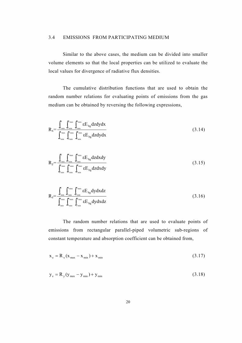
3.4 EMISSIONS FROM PARTICIPATING MEDIUM

Similar to the above cases, the medium can be divided into smaller

volume elements so that the local properties can be utilized to evaluate the

local values for divergence of radiative flux densities.

The cumulative distribution functions that are used to obtain the

random number relations for evaluating points of emissions from the gas

medium can be obtained by reversing the following expressions,

Rx=∫ ∫ ∫∫ ∫ ∫

max

min

max

min

max

min

min

max

min

max

min

x

x

y

y

z

z bg

x

x

y

y

z

z bg

dzdydxεE

dzdydxεE (3.14)

Ry=∫ ∫ ∫∫ ∫ ∫

max

min

max

min

max

min

min

max

min

max

min

y

y

x

x

z

z bg

y

y

x

x

z

z bg

dzdxdyεE

dzdxdyεE (3.15)

Rz=∫ ∫ ∫∫ ∫ ∫

max

min

max

min

max

min

min

max

min

max

min

z

z

x

x

y

y bg

z

z

x

x

y

y bg

dydxdzεE

dydxdzεE (3.16)

The random number relations that are used to evaluate points of

emissions from rectangular parallel-piped volumetric sub-regions of

constant temperature and absorption coefficient can be obtained from,

minminmaxxe x)x(xRx +−= (3.17)

minminmaxye y)y(yRy +−= (3.18)

20

minminmaxze z)z(zRz +−= (3.19)

where xe, ye and ze are the points of emissions, xmax, ymax, zmax, xmin, ymin and

zmin are the maximum and minimum coordinates of a parallelepiped

volumetric sub-region in terms of rectangular coordinate variables x, y, and

z, respectively.

Similar to the surface emissions, the temperature throughout the

whole sub-region can be assumed equal to a representative temperature

value even if there is a temperature variation within the sub-region.

The points of emission can also be selected from a uniform

distribution without generating any random number.

The azimuthal angle of the emitted photon bundle can still be

evaluated from Eq. (3.12) while the polar angle shown in Fig. 3.1 can be

obtained by using Eq. (3.20). The change in the random number relation for

the polar angle is due to the change in integration limits from 0 to π/2 for

the surface emissions, and from – π/2 to π/2 for volumetric gas emission,

Figure 3-1 The polar angle in participating medium

21

)2R-arccos(1θ θ= (3.20)

The evaluation of the wave number with a random number relation is

usually more complicated than the evaluation of the preceding random

number relation because the spectral variation of the participating medium

is defined by more complicated equations than those of points or directions

of emission. The cumulative distribution function for the wave number is

given by,

Rη(η)=∫∫∞

ηη

ηη

ηκ

ηκ

0 b

1

0 b

dE

dE (3.21)

where the spectral absorption coefficient, and Ebη is the spectral

blackbody emissive power of the medium.

ηκ

The cumulative distribution function obtained by Eq. (3.21) can be

usually inverted by numerical methods to obtain wave number random

relation,

η=η(Rη) (3.22)

3.5 RAY TRACING

During the simulation, the step following the evaluation of points of

emission and wavelength is the evaluation of the direction of the photon

bundle by using the random number relations for polar and azimuthal angles.

As shown in Fig. 3-2, the unit direction vector represented by the

polar angle θ measured from the surface normal, and the azimuthal angle ψ

22

measured from t 1 can be calculated by,

s = [ ncostsint)sin(sinsin

21 θ+ψ+ψ−ααθ ] (3.23)

where α is the angle between t 1 and t 2. For the rectangular coordinate

system, which is the coordinate system used throughout this study, α = π /2,

and the Eq. (3.23) reduces to,

s = [ ] ncosθtsinψtcosψsinθ 21 ++ (3.24)

The photon bundle can then be traced until it is absorbed by the gas

medium or by a surface it collides with. Different ray tracing algorithms

simulating the physical events with different statistical approaches can be

utilized.

Figure 3-2 Vector description of emission direction and point of

incidence (Modest [30])

23

Ray tracing Algorithm:

Assuming that medium is transparent, the point →r on a surface that

the photon bundle emitted at location will collide with and the

corresponding distance L

er→

w that the photon bundle will travel before this

collision, is found by using,

er→

+Lw s = (3.25) wr→

When rectangular coordinate system is considered, Eq. (3.25) can be written

in terms of x, y, z components and solved for Lw by forming the dot

products with unit vectors of rectangular coordinate system, ˆ , , and i j k ,

Lw=i.sxx e− =

j.syy e− =

k.szz e− (3.26)

Eq. (3.26) is a set of three equations, in the three unknowns, Lw, and two of

the coordinates, where the third coordinate is defined in terms of the other

two by using the surface equation. If more than one intersection is a

possibility (in the presence of convex surfaces, etc.), then the path lengths

Lw, for all possibilities are determined, the correct one is the one that gives

the shortest possible path.

Having the wave number evaluated, the mean free path which is the

distance that a photon bundle will travel before being absorbed by the gas

medium, for the case in which the absorption coefficient does not vary

throughout the medium (κη=constant), can be calculated by using,

Lκ=

κη R1ln

κ1 (3.27)

24

If the absorption coefficient is not uniform, which can be due to

temperature dependence or anisotropic medium, the optical path is evaluated

by breaking up the volume into n sub-volumes each with a constant

absorption coefficient.

∫ ∑≅1

0n

nηnη lκdsκ (3.28)

The summation in Eq. (3.28) is over the n sub-volumes through which the

bundle has traveled, and ln is the distance the bundle travels through in

element n. The bundle is not absorbed and is allowed to travel on as long as

the following condition holds,

∫ ∫ =<1

0

L

0κ

ηηκ

R1lndlκdlκ (3.29)

If the scattering coefficient does not vary throughout the medium, the

distance that a photon bundle will travel before it is scattered can be

evaluated by using,

Lσ=

ση R1nl

σ1 (3.30)

For a medium with variable scattering coefficient, the following

condition holds:

∫ ∑ ∫σ

ηηη =σ<σ≅σ σ1

0n

L

0nn R1lndlldl (3.31)

25

After having all Lκ, Lσ, and Lw in one hand, the three lengths can be

compared to understand whether the bundle will be scattered by the gas,

absorbed in the gas, or hits a wall. If Lw is the smallest of all, the bundle

directly collides with the wall without being scattered or absorbed by the

gas. Then, the absorptivity of the wall is compared with a generated random

number. If the random number is smaller than the absorptivity, the wall

absorbs the bundle. Otherwise, the bundle is reflected from the wall. If the

surface is a diffuse reflector, angles of reflection can be calculated from the

following expressions:

θr=arcsin( rRθ ) (3.32)

ψr=2 (3.33) rψπR

If Lκ is the smallest, the gas absorbs the bundle. On the other hand,

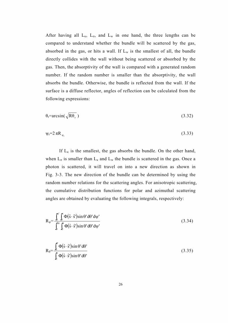
when Lσ is smaller than Lκ and Lw the bundle is scattered in the gas. Once a

photon is scattered, it will travel on into a new direction as shown in

Fig. 3-3. The new direction of the bundle can be determined by using the

random number relations for the scattering angles. For anisotropic scattering,

the cumulative distribution functions for polar and azimuthal scattering

angles are obtained by evaluating the following integrals, respectively:

Rψ=( )

( )∫ ∫∫ ∫

ψθθ⋅

ψθθ⋅Φπ

2π

0

π

0

ψ'

0 0

'd'd'sin'ssΦ

'd'd'sin'ss (3.34)

Rθ=( )

( )∫∫π

θθ⋅

θθ⋅

0

θ'

0

'd'sin'ssΦ

'd'sin'ssΦ (3.35)

26

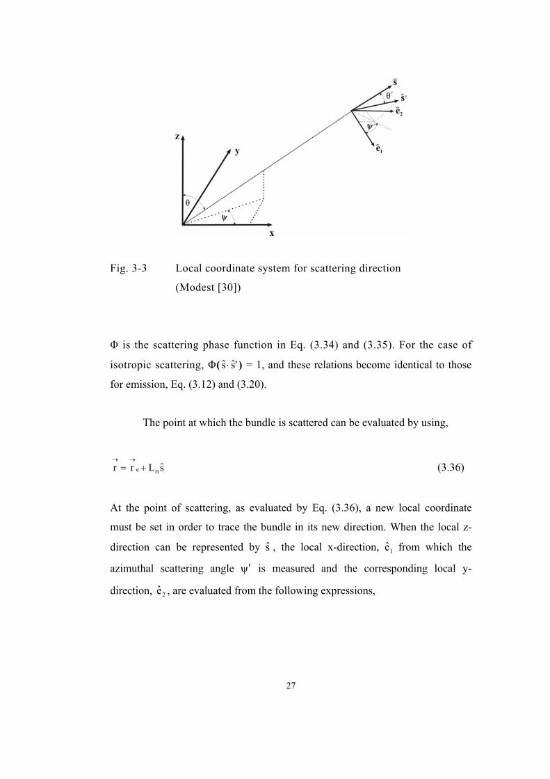
Fig. 3-3 Local coordinate system for scattering direction

(Modest [30])

Φ is the scattering phase function in Eq. (3.34) and (3.35). For the case of

isotropic scattering, Φ( ' ) = 1, and these relations become identical to those

for emission, Eq. (3.12) and (3.20).

ss ⋅

The point at which the bundle is scattered can be evaluated by using,

sLrr e σ

→→+= (3.36)

At the point of scattering, as evaluated by Eq. (3.36), a new local coordinate

must be set in order to trace the bundle in its new direction. When the local z-

direction can be represented by , the local x-direction, from which the

azimuthal scattering angle

s 1e

ψ′ is measured and the corresponding local y-

direction, , are evaluated from the following expressions, 2e

27

1e =sa

sa

×

×→

→

(3.37)

2e = (3.38) 1es×

In Eq. (3.37), is any arbitrary vector. Similar to Eq. (3.24), the new

direction vector is expressed by

→

a

's = [ ] s'θcoseψ'sine'ψcos'sin 21 ++θ (3.39)

Then, the new distance, Lw, that the bundle will travel before hitting

a surface is evaluated from Eq. (3.26) by replacing the coordinates of point

of emission by coordinates of point of scattering. The path that the bundle

will travel before it is absorbed by gas, Lκ, can be calculated by reducing the

traveled path from the value evaluated before. Based on the values obtained

by a similar procedure, the photon bundle is traced until it hits a surface and

absorbed by it, or until a gas volume absorbs it.

A similar ray tracing procedure continues until the gas or one of the

surfaces absorbs the bundle, where the history is terminated. Then, a new

history starts with the emission of a new bundle. The simulation continues

until the whole energy that is generated and recovered in the system is

considered.

28

CHAPTER 4

APPLICATIONS OF MONTE CARLO METHOD TO

SURFACE EXCHANGE PROBLEMS

Monte Carlo method is first applied to surface exchange problems so

that the general characteristics of the method can be understood in simpler

problems before the method is applied to more complex problems involving

three-dimensional geometries and participating media.

The surface exchange problems can be considered in two different

categories. The first is evaluation of view factors of certain geometries and

the second is evaluation of the net radiation exchange between a number of

black and grey surfaces.

4.1 EVALUATION OF VIEW FACTORS

The view factor Fij is defined as the fraction of radiation leaving

surface i, which is intercepted by surface j. The general expression that

gives the view factor for two surfaces that are diffuse emitters and reflectors

and have uniform radiosity is given in Eq. (4.1),

Fij= ∫ ∫ π

θ⋅θ

j iA A ji2ji

idAdA

Scoscos

A1 (4.1)

29

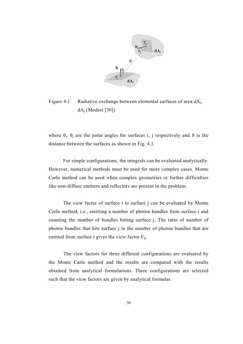
Figure 4.1 Radiative exchange between elemental surfaces of area dAi,

dAj (Modest [30])

where θi, θj are the polar angles for surfaces i, j respectively and S is the

distance between the surfaces as shown in Fig. 4.1.

For simple configurations, the integrals can be evaluated analytically.

However, numerical methods must be used for more complex cases. Monte

Carlo method can be used when complex geometries or further difficulties

like non-diffuse emitters and reflectors are present in the problem.

The view factor of surface i to surface j can be evaluated by Monte

Carlo method, i.e., emitting a number of photon bundles from surface i and

counting the number of bundles hitting surface j. The ratio of number of

photon bundles that hits surface j to the number of photon bundles that are

emitted from surface i gives the view factor Fij.

The view factors for three different configurations are evaluated by

the Monte Carlo method and the results are compared with the results

obtained from analytical formulations. Three configurations are selected

such that the view factors are given by analytical formulas.

30

The first selected configuration is two aligned, parallel, equal

rectangles as shown in Fig.4.2,

Figure 4.2 Two aligned, parallel, and equal rectangles (Modest [30])

The view factor F12 for the configuration under consideration is

calculated by Monte Carlo method, and is compared with the analytical

solution given by the following expression:

+++

+++⋅+

= −1/22

11/221/2

22

22

12 )Y(1Xtan)Y(1X

YX1)Y(1)X(1ln

XYπ2F

YtanYXtanX)X(1

Ytan)X(1Y 112

11/22 −−− −−

+++ (4.2)

In Eq. (4.2), c/aX = and c/bY = .

The points of emission are calculated by Eq. (3.9) and (3.10); the

azimuthal and polar angles of the emitted photon bundles are obtained by Eq.

(3.12), (3.13), respectively.

31

)a.(Rx xe = (4.3)

)b.(Ry ye = (4.4)

ψπ=ψ R2 (4.5)

)Rarcsin( θ=θ (4.6)

where Rx, Ry, Rψ, and Rθ are random numbers.

As the distance c is fixed, the points of the bundles passing through at the

plane of surface 2 can be evaluated as,

x= xe +c.tanθ.cosψ (4.7)

y=ye + c.tanθ.sinψ (4.8)

where ψ is measured from positive x-axis and θ is measured from positive z-

axis.

If x and y coordinates which are calculated by Eq. (4.7) and (4.8), are in

the area bounded by surface 2, the counter for the hits on surface 2 is

increased by one. After a number of photon bundles are emitted from

surface 1, the view factor F12 can be evaluated.

The second configuration selected is perpendicular rectangles with an

equal common edge as shown in Fig. 4.3.

32

Figure 4.3 Perpendicular rectangles with an equal common edge (Modest

[30])

The view factor F12 calculated by Monte Carlo method is compared with

the analytical solution given by the following expression,

++−+

π= −−−

2/12212/12211

12 )WH(1tan)WH(

H1tanH

W1tanW

W1F

2w

222

222

22

22

)HW)(W1()HW1(W

HW1)H1)(W1(ln

41

++++

++++

+

++++

×

2H

222

222

)WH)(H1()WH1(H (4.9)

where H = h/l and W = w/l in Eq. (4.9).

The points of emissions from surface 1 are calculated by Eq. (3.9) and

(3.10). The azimuthal and polar angles of the emitted photon bundles are

obtained from Eq. (3.12), (3.13), respectively, just like the first case. This

time, the x-coordinate of the plate 2 is fixed and the points of the bundles

passing through at the plane of surface 2 can be evaluated by,

)w.(Rx xe = (4.10)

33

)l.(Ry ye = (4.11)

y= (4.12) ψ− tanxy ee

z = ze - (ψθ cos tan

x e ) (4.13)

As it is done in the first case, if y and z coordinates which are calculated

by Eq. (4.12) and (4.13) are in the area bounded by surface 2, the counter of

the hits on surface 2 is increased by one. After a number of photon bundles

is emitted from surface 1, the view factor F12 can be evaluated.

The third configuration selected is parallel co-axial discs as shown in

Fig. 4.4

The view factor F12 calculated by Monte Carlo method was compared

with the analytical solution given by the following expression,

−−=

2

2

1212 R

R4XX

21F (4.14)

Figure 4.4 Parallel co-axial discs (Modest [30])

34

In Eq. (4.14), , h/rR 11 = h/rR 22 = and . 212

2 R/)R1(1X ++=

The points of emission from surface 1 are calculated by Eq. (3.9), the

azimuthal and polar angles of the emitted photon bundles are obtained by Eq.

(3.12), (3.13), respectively. The points of locations of the bundles passing

through at the plane of surface 2 can be evaluated by,

)r.(Rr 1re = (4.14)

r = )))cos(tanhr.(2)r()tan.h(( e2

e2 ψ−π⋅θ⋅⋅−+θ (4.15)

If r calculated by Eq. (4.15) is in the area bounded by surface 2, the

counter of the hits on surface 2 is increased by one. After a number of

photon bundles are emitted from surface 1, the view factor F12 can be

evaluated.

Variance reduction can be applied to reduce computation time in each

case by selecting azimuthal angles within range of interest between θmax and

θmin, or ψmax and ψmin, instead of selecting θ between 0 and π/2 and ψ

between 0 and 2π, respectively. Then, Eq. (3.12) and (3.13) used to define

the direction of the emitted photon bundles become,

minminmax )(R ψ+ψ−ψ=ψ ψ (4.16)

))sin)sin(sinRarcsin( min2

min2

max2 θ+θ−θ=θ θ (4.17)

The ratio of number of photon bundles that hits surface 2 to the number

of photon bundles that is emitted from surface 1 is multiplied by

(ψmax- ψmin)/2π when azimuthal angle is used with variance reduction, and is

35

multiplied by ( - ) when polar angle is used with variance

reduction, to obtain the view factor F

max2sin θ min

2sin θ

12.

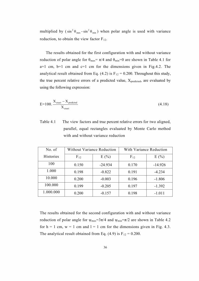
The results obtained for the first configuration with and without variance

reduction of polar angle for θmax= π/4 and θmin=0 are shown in Table 4.1 for

a=1 cm, b=1 cm and c=1 cm for the dimensions given in Fig.4.2. The

analytical result obtained from Eq. (4.2) is F12 = 0.200. Throughout this study,

the true percent relative errors of a predicted value, Xpredicted, are evaluated by

using the following expression:

E=100.exact

predictedexact

XXX −

(4.18)

Table 4.1 The view factors and true percent relative errors for two aligned,

parallel, equal rectangles evaluated by Monte Carlo method

with and without variance reduction

Without Variance Reduction With Variance Reduction No. of

Histories F12 E (%) F12 E (%)

100 0.150 -24.934 0.170 -14.926 1.000 0.198 -0.822 0.191 -4.234

10.000 0.200 -0.003 0.196 -1.806 100.000 0.199 -0.205 0.197 -1.392

1.000.000 0.200 -0.157 0.198 -1.011

The results obtained for the second configuration with and without variance

reduction of polar angle for ψmax=3π/4 and ψmin=π/2 are shown in Table 4.2

for h = 1 cm, w = 1 cm and l = 1 cm for the dimensions given in Fig. 4.3.

The analytical result obtained from Eq. (4.9) is F12 = 0.200.

36

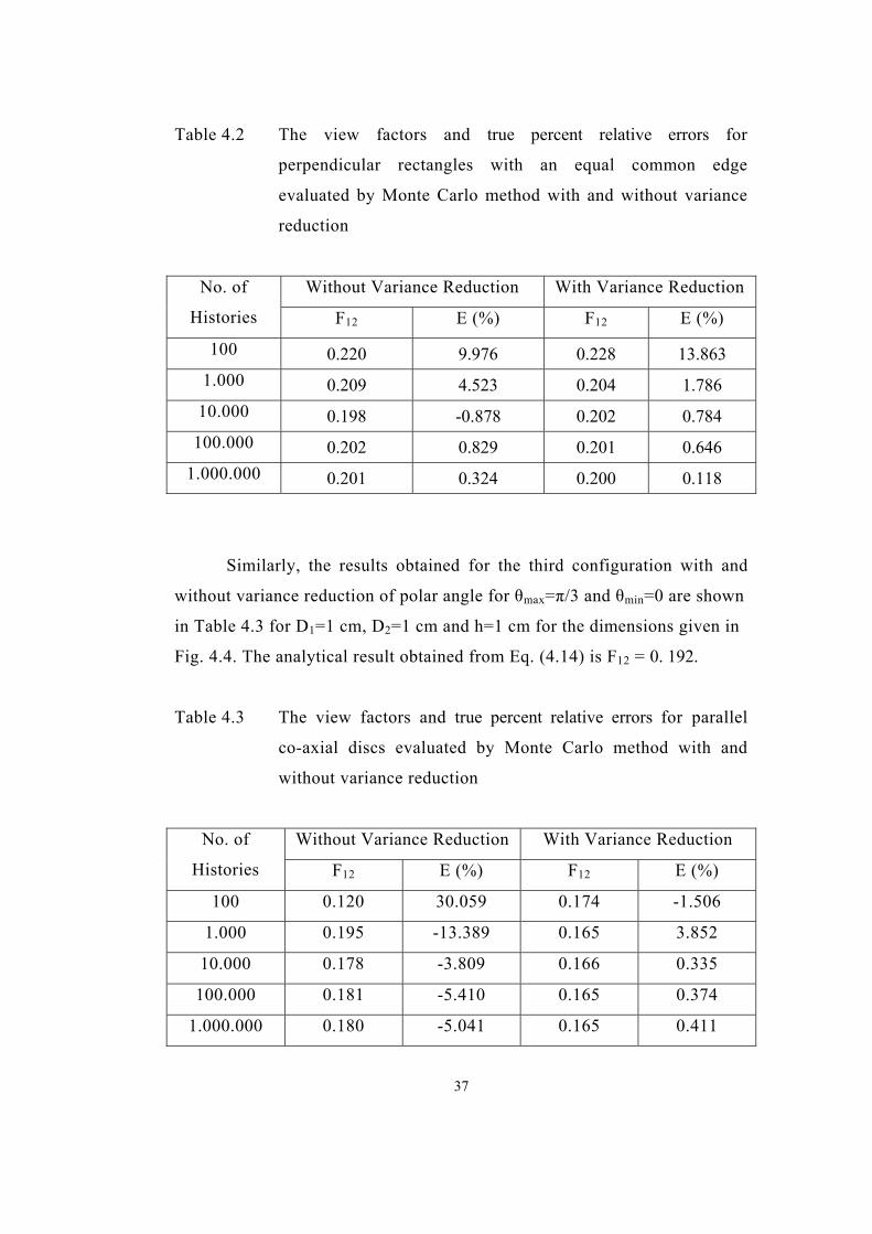
Table 4.2 The view factors and true percent relative errors for

perpendicular rectangles with an equal common edge

evaluated by Monte Carlo method with and without variance

reduction



100 0.220 9.976 0.228 13.863 1.000 0.209 4.523 0.204 1.786

10.000 0.198 -0.878 0.202 0.784 100.000 0.202 0.829 0.201 0.646

1.000.000 0.201 0.324 0.200 0.118

Similarly, the results obtained for the third configuration with and

without variance reduction of polar angle for θmax=π/3 and θmin=0 are shown

in Table 4.3 for D1=1 cm, D2=1 cm and h=1 cm for the dimensions given in

Fig. 4.4. The analytical result obtained from Eq. (4.14) is F12 = 0. 192.

Table 4.3 The view factors and true percent relative errors for parallel

co-axial discs evaluated by Monte Carlo method with and

without variance reduction



100 0.120 30.059 0.174 -1.506

1.000 0.195 -13.389 0.165 3.852

10.000 0.178 -3.809 0.166 0.335

100.000 0.181 -5.410 0.165 0.374

1.000.000 0.180 -5.041 0.165 0.411

37

When we examine all the tables of results, it can be said that variance

reduction produces results that are more accurate when small number of

photon histories are used. However, Monte Carlo method without variance

reduction also predicts accurate results when we use high number of photon

histories.

Therefore, we can conclude that variance reduction is useful method

when we use small N (# of photon bundle history). In addition, when one of

the dimensions of the geometry is very small or greater than the other

dimensions, variance reduction gives better results than without using

variance reduction. On the other hand, there is a criterion for variance

reduction. The determination of at what angles we are going to restrict the

angles to hit the second surface is a critical issue, and it affects the results

very significantly. Therefore, the angles must be chosen carefully when the

variance reduction technique is used.

4.2 EVALUATION OF NET RADIATION EXCHANGE

If the two black surfaces in Fig. 4.1 is considered, the radiation

leaving surface i and intercepted by surface j is,

jiq → = FijAiσTi4 (4.19)

Similarly, the radiation leaving the surface j and intercepted by

surface i is,

ijq → =FjiAjσTj4 (4.20)

From the reciprocity relation, it is known that,

38

AiFij = AjFji (4.21)

Then, the net radiation exchange between the two black surfaces can

be formulated as,

qij= - =Fjiq → ijq → ijAiσ(Ti4-Tj

4) (4.22)

For simple geometric configurations and simple radiative properties

such as black walls and diffuse emitters and reflectors, the problem of

radiation exchange is simple and can be easily handled with analytical

methods. But, when further complications arise such as complex geometries

and non-grey or non-diffuse surfaces, numerical methods must be used.

Application of the Monte Carlo method to net radiation exchange

problems is very similar to the application of the method for determination

of the view factor problems. The main difference is, for the surface

exchange problems, the photon bundles are considered to carry some

amount of energy specified by Eq. (3.1). This energy is transmitted to the

other surface when the emitted photon bundle hits a surface and is absorbed

by that surface. The net radiative heat transferred to a surface can be found

when all the surfaces emit some number of photon bundles with some

energy assigned to each of the bundle, and calculating the difference

between the energy emitted from the surface and energy absorbed by the

surface.

4.3 EVALUATION OF NET RADIATION EXCHANGE BETWEEN

BLACK SURFACES

The net radiation exchange problems are solved for the two

rectangular box configurations as shown in Figs. 4.5 and 4.6, and the results

39

obtained by using different numbers of photon bundle histories are

compared with the results of analytical formulation.

Analytical solution of radiative heat exchange between isothermal black

surfaces are obtained as,

qi= , i=1,2,...,N. (4.23) ( )∑=

− −−N

1joibjbiji HEEF

Figure 4.5 Configuration 1

Figure 4.6 Configuration 2

40

During the solutions, the number of photon bundles emitted from each

isothermal surface is kept constant while the energy of each emitted photon

bundle is taken to be directly proportional to the emissive power of the point

of emission. Based on this assumption, energy of the photon bundles

emitted from each plate is directly proportional to the fourth power of the

absolute temperature of the plate, evaluated from Eq. (3.1).

The net radiative heat exchange between the surfaces is calculated for

the enclosures shown in Fig. 4.5 and 4.6. Temperature values of the surfaces

are the same as the problems in participating medium that will be discussed

in the following chapters. The solutions that are obtained with different

number of histories are presented in Tables 4.4., 4.5 and 4.6 for

Tbottom=1149 K, Ttop=822 K and Tlateral=1059 K. The analytical results and

true percent relative errors are obtained by Eq. (4.23) and Eq. (4.18),

respectively.

Table 4.4 The net radiative heat exchange for bottom surface

Bottom Surface

Configuration 1 Configuration 2

qexact=3.56X104 W qexact=5.42X103 W

No. of

Histories

from bottom

surface qMC(W) Err.(%) qMC(W) Err.(%)

100 4.06 X104 -14.26 6.03 X103 -11.3

1.000 3.56 X104 0.01 4.52 X103 16.5

10.000 3.51 X104 1.37 5.10 X103 5.8

100.000 3.57 X104 -0.33 5.50 X103 -1.6

1.000.000 3.55 X104 0.31 5.40 X103 0.3

41

Table 4.5 The net radiative heat exchange for top surface

Top Surface


qexact=-5.07X104 W qexact=-9.23X103 W

No. of

Histories

from top


100 -5.14 X104 -1.41 -4.43 X103 52.0

1.000 -4.75 X104 6.26 -6.07 X103 34.2

10.000 -5.11 X104 -0.75 -8.67 X103 6.0

100.000 -5.05 X104 0.49 -9.16 X103 0.8

1.000.000 -5.06 X104 0.18 -9.21 X103 0.2

Table 4.6 The net radiative heat exchange for lateral surface

Lateral Surface



No. of

Histories

from lateral


400 1.08 X104 28.7 -1.59 X103 141.8

4.000 1.19 X104 20.9 1.55 X103 59.4

40.000 1.60 X104 -5.73 3.57 X103 6.3

400.000 1.48 X104 2.43 3.65 X103 4.2

4.000.000 1.52 X104 -0.12 3.81 X103 0.1

From the results, it can be concluded that the Monte Carlo algorithms

are validated for the simple view factor and radiative heat exchange

problems. The verified algorithms can be modified for problems with more

complex geometries and radiative problems, but as the aim of the study is to

42

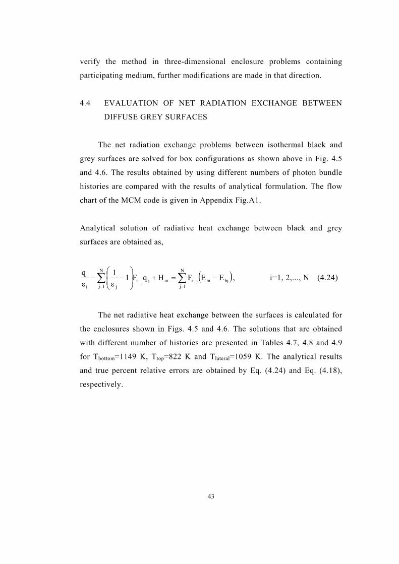
verify the method in three-dimensional enclosure problems containing

participating medium, further modifications are made in that direction.

4.4 EVALUATION OF NET RADIATION EXCHANGE BETWEEN

DIFFUSE GREY SURFACES

The net radiation exchange problems between isothermal black and

grey surfaces are solved for box configurations as shown above in Fig. 4.5

and 4.6. The results obtained by using different numbers of photon bundle

histories are compared with the results of analytical formulation. The flow

chart of the MCM code is given in Appendix Fig.A1.

Analytical solution of radiative heat exchange between black and grey

surfaces are obtained as,

( )∑∑=

−=

− −=+

−

ε−

ε

N

1jbjbiji

N

1joijji

ji

i EEFHqF11q , i=1, 2,..., N (4.24)

The net radiative heat exchange between the surfaces is calculated for

the enclosures shown in Figs. 4.5 and 4.6. The solutions that are obtained

with different number of histories are presented in Tables 4.7, 4.8 and 4.9

for Tbottom=1149 K, Ttop=822 K and Tlateral=1059 K. The analytical results

and true percent relative errors are obtained by Eq. (4.24) and Eq. (4.18),

respectively.

43

Table 4.7 The net radiative heat exchange for bottom surface

Bottom Surface



ε1=0.33 ε2=0.33 εlateral=0.33 ε1=0.33 ε2=0.33 εlateral=0.33

No. of

Histories

from bottom


100 4.87X103 53.0 -6.80X102 137.7

1.000 9.56X103 7.6 1.04X103 42.5

10.000 9.92X103 4.1 1.47X103 18.7

100.000 1.00X104 3.0 1.58X103 12.5

1.000.000 1.01X104 2.7 1.62X103 10.1

Table 4.8 The net radiative heat exchange for top surface

Top Surface


qexact=-1.48X104 W qexact=-3.01X103 W


No. of

Histories

from top


100 -1.15X104 22.0 -4.57X103 51.9

1.000 -1.42X104 4.1 -2.75X103 8.7

10.000 -1.44X104 2.4 -2.85X103 5.4

100.000 -1.44X104 2.1 -2.73X103 9.2

1.000.000 -1.45X104 1.7 -2.78X103 7.9

44

Table 4.9 The net radiative heat exchange for lateral surface

Lateral Surface




No. of

Histories

from lateral


400 6.64X103 -50.7 5.25X103 -334.5

4.000 4.59X103 -4.2 1.71X103 -41.8

40.000 4.49X103 -1.8 1.38X103 -14.4

400.000 4.41X103 0.1 1.16X103 4.4

4.000.000 4.44X103 -0.7 1.15X103 4.7

When we examine the net radiative heat exchange between the

surfaces inside the rectangular enclosure, it can be seen from the tables that

Monte Carlo method gives accurate results for a cubic enclosure. However,

the results for Configuration 2 (Fig. 4.6) are not as accurate as that of a

cubic enclosure.

The photons emitted from and absorbed at the bottom and top surfaces

have important weight in the solution. The reflectivity (ρ) values of opaque

and diffuse walls are equal to (1-α) where α (absorptivity) equals to ε

(emissivity) value. Low emissivity values leads to high reflectivity values.

Therefore, emitted photons make high number of reflections in the

enclosure because of low emissivity values of the walls. Then, high

reflections of the photons in the enclosure and thin-long geometry of the

configuration 2 affect the number of photons absorbed at the bottom and top

surfaces. Smaller or larger number of absorptions at the walls than the

expected is the main reason of high error values at the top and bottom

45

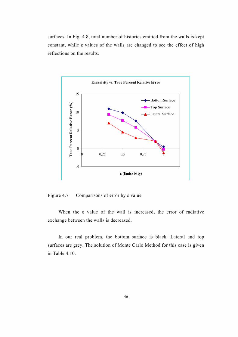
surfaces. In Fig. 4.8, total number of histories emitted from the walls is kept

constant, while ε values of the walls are changed to see the effect of high

reflections on the results.

Emissivity vs. True Percent Relative Error

-5

0

5

10

15

0 0,25 0,5 0,75 1

ε (Emissivity)

Tru

e Pe

rcen

t Rel

ativ

e E

rror

(%) Bottom Surface

Top Surface

Lateral Surface

Figure 4.7 Comparisons of error by ε value

When the ε value of the wall is increased, the error of radiative

exchange between the walls is decreased.

In our real problem, the bottom surface is black. Lateral and top

surfaces are grey. The solution of Monte Carlo Method for this case is given

in Table 4.10.

46

Table 4.10 The net radiative heat exchange for real problem

Configuration 2

ε1=1.0 ε2=0.87 εlateral=0.33

Bottom Surface Top Surface Lateral Surface

qexact=5.57X103 W qexact=-7.89X103 W qexact=2.33X103 W

Total no. of

history used

in the

enclosure qMC(W) Err(%) qMC(W) Err(%) qMC(W) Err(%)

1.312.141 4.09X103 26.6 -6.26X103 20.7 2.17X103 6.5

13.121.417 4.12X103 26 -6.28X103 20.4 2.16X103 7.1

350.000.000 4.17X103 26 -6.28X103 20.4 2.17X103 6.9

In order to decrease the error, variance reduction technique is applied

to the enclosure. The number of emitted photons is proportional to the area

of the surface when we use uniform distribution of point of emission.

The volume near the bottom and top has important weight in the

solutions. Near the bottom, the bottom surface absorbs larger number of

photons than expected. Moreover, the top surface absorbs a smaller number

of photons than expected due to the thin-long geometry of the enclosure as

shown in Fig. 4.6 and high reflections in the enclosure. The photons, which

are emitted from the top, bottom and lateral surfaces, are confined in the

lateral zone and have little chance to go to the top and bottom surfaces. In

order to eliminate this problem, biasing is used instead of direct simulation.

The number of photons emitted from important regions is increased.

The lateral zone is divided into three parts as shown in Fig. 4.9. For

two situations, the properties of the lateral zones are given in Table 4.11.

The definitions of ARx and PRx, which are used in Table 4.11, are,

47

ARx=surface lateral of Area

X zone lateral of Area (4.25)

PRx= surface lateral from photons emitted of # Total

X zone lateral from photons emitted of # Total (4.26)

Figure 4.8 Lateral surface in three zones

48

Table 4.11 The lateral zone area and total number of emitted photons

ratios for biasing

AR1 PR1 AR PR2 AR PR3

Biasing # 1

L1=0.45 m L2=2.45 m L3=0.45 m

13.43 10.00 73.14 72.50 13.43 17.50

Biasing # 2

L1=0.90 m L2=1.55 m L3=0.90 m

26.87 15.75 46.26 56.15 26.87 28.1

2 3

The net radiative heat exchange is analyzed for the problems under

consideration. As the bottom surface absorbs a larger number of photons

than expected, total emitted number of photons from lateral zone 1 is

decreased. Similarly, emitted number of photons from lateral zone 3 is

increased because the top surface absorbs a smaller number of photons than

expected.

Table 4.12 Biasing #1

ε1=1.0 ε2=0.87 εlateral=0.33


Total no. of

history used

in the

enclosure Error (%) Error (%) Error (%)

2.500.000 -0.55 -0.62 -0.76

3.000.000 -0.77 -0.10 1.52

15.000.000 -0.76 -0.28 0.86

49

Table 4.13 Biasing #2

ε1=1.0 ε2=0.87 εlateral=0.33


Total no. of

history used

in the

enclosure Error (%) Error (%) Error (%)

1.000.000 2.08 0.90 -1.93

2.500.000 1.28 0.27 -2.17

3.000.000 0.70 0.42 -0.26

When we examine Tables 4.12 and 4.13, we may conclude that

biasing produces good results. By increasing the number of photons emitted

from zone 3, the number of absorbed photons at the top surface is increased.

On the contrary, by decreasing the number of photons emitted from zone 1,

the number of absorbed photons at the bottom surface is decreased.

The geometry of the enclosure is difficult for ray tracing applications.

In order to eliminate this difficulty, biasing should be applied.

50

CHAPTER 5

APPLICATION OF MONTE CARLO METHOD TO

PROBLEMS WITH PARTICIPATING MEDIUM

The difficulties in radiative transfer problems arise with interaction

of thermal radiation with an absorbing, emitting and scattering medium.

When participating medium is considered, the radiative transfer equation

describes the radiative intensity field within the enclosure as a function of

location, direction and spectral variable,

( ) ( ) ( ) ( ) ( )∫π

ηηη

ηηηηη Ω′′Φη′π

σ+ηβ−ηκ=η∇⋅

4

sb ds,s,s,rI

4,s,rI,s,rI,s,rIs

rrrrr (5.1)

where, Iη is the radiation intensity in the direction , at the position s rr ,

defined as the quantity of radiant energy passing in specified direction

along a path per unit solid angle, per unit area normal to the direction of

travel, per unit time. κ, σ

s

s and β are the absorption, scattering and extinction

coefficients of the medium, respectively. Ibη is the blackbody radiation

intensity, and ( )s,s′Φη is the scattering phase function, which describes the

fraction of energy scattered from incoming direction to outgoing

direction s . The expression on the left-hand side represents the change of the

intensity in the specified direction s . The terms on the right-hand side stand

for emission, extinction, and in-scattering, respectively.

s′

ˆ

ˆ

51

In order to obtain the net radiation heat flux crossing a surface

element, the contributions of radiative energy irradiating the surface from

all possible directions and over all possible wave lengths must be summed

up. Therefore, integrating the equation of transfer over all directions and all

wave lengths leads to a conservation of radiative energy statement applied

to an infinitesimal volume. It is impossible to handle these integrals by

analytical means in most of the problems when the radiative properties are

functions of location, direction and spectral variable at the same time.

When these difficulties arise coupled with multi-dimensional

complex geometries, the approximate solution methods are used to evaluate

the radiative heat fluxes subjected to the surfaces and divergence of

radiative heat flux subjected to the medium. Monte Carlo method finds its

main application area in problems of radiative transfer when participating

medium and complex multi-dimensional geometries are considered.

In this study, the Monte Carlo method is applied to two enclosure

problems to validate the accuracy. The first one is a 3-D cubical enclosure

problem, which has numerical solutions [24]. The second one is a box-

shaped enclosure problem. The comparisons will be made between

experimental measurements and numerical solutions [26].

5.1 3-D CUBICAL ENCLOSURE PROBLEM CONTAINING

SCATTERING MEDIUM

Most engineering problems are in fact non-ideal problems where

simplifications are needed to obtain references to compare with the

idealized cases and give rise to develop numerical solution techniques. The

idealized problem studied in this part is a 3-D cubical enclosure containing

uniform, grey, isotropically and anisotropically scattering medium bounded

52

by diffuse, grey walls (Fig. 5.1). In this idealized problem, two cases are

analyzed. The first cubical enclosure case is a purely scattering medium

with non-symmetric boundary conditions. The second problem is

characterized by an isothermal, absorbing, emitting, scattering medium and

symmetric boundary conditions. The specified parameters of these problems

are presented in Table 5.1. κ*, σs* and β* are non-dimensional radiative

properties defined as κ*= κ.Lo, σs*

= σs.Lo, β*= β.Lo where Lo is the dimension

of the cubical enclosure. The flow chart of the MCM code for this case is

given in Appendix Fig.A2.

Fig. 5.1 Coordinate system for cubical enclosure problems [25]

53

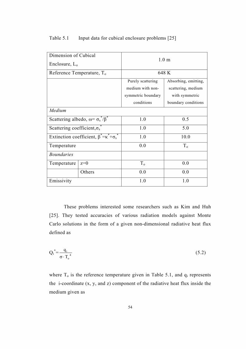
Table 5.1 Input data for cubical enclosure problems [25]

Dimension of Cubical

Enclosure, Lo 1.0 m

Reference Temperature, To 648 K

Purely scattering

medium with non-

symmetric boundary

conditions

Absorbing, emitting,

scattering, medium

with symmetric

boundary conditions Medium

Scattering albedo, ω= σs*/β* 1.0 0.5

Scattering coefficient,σs* 1.0 5.0

Extinction coefficient, β*=κ*+σs* 1.0 10.0

Temperature 0.0 To

Boundaries

Temperature z=0 To 0.0

Others 0.0 0.0

Emissivity 1.0 1.0

These problems interested some researchers such as Kim and Huh

[25]. They tested accuracies of various radiation models against Monte

Carlo solutions in the form of a given non-dimensional radiative heat flux

defined as

Qi*= 4

o

i

Tq⋅σ

(5.2)

where To is the reference temperature given in Table 5.1, and qi represents

the i-coordinate (x, y, and z) component of the radiative heat flux inside the

medium given as

54

qi= (5.3) ( )∫π

Ω⋅⋅Ω⋅4

i dIe

where ei is the unit normal vector in the coordinate direction i.

The scattering phase functions used to examine the effects of

anisotropy in both problems are those given by Kim et al. [31]. The phase

function Φ( , ), which represents the fraction of energy scattered into the

outgoing direction s from the incoming direction

s′ s

ˆ s′ , is approximated by a

finite series of Legendre polynomials as follows

Φ( s , )= Φ(Cosθ)= (5.4) ˆ′ s (∑=

θ⋅N

0jjj CosPC )

where Pj’s are the Legendre polynomials of order j defined as

P0 = 1

P1 = x (5.5)

Pj = ( ) ( )xPj1jxPx

j1j2

1j1j −− ⋅−

−⋅⋅−⋅

Cj’s are the expansion coefficients and θ is the angle between incoming and

outgoing directions.

Phase functions described by the expansion coefficients listed in

Table 5.2 and illustrated in Fig. 5.2 are used in this study. The phase

function F2 is for forward, and B2 is for backward scattering. Phase

functions are shown in Figs. 5.3-5.5.

55

Table 5.2 Expansion coefficients for phase functions [31]

C

j F2 B2

0 1.00000 1.00000

1 2.00917 -1.20000

2 1.56339 0.50000

3 0.67407

4 0.22215

5 0.04725

0.00671

7 0.00068

8 0.00005

j

6

Fig. 5.2 Phase functions [31]

56

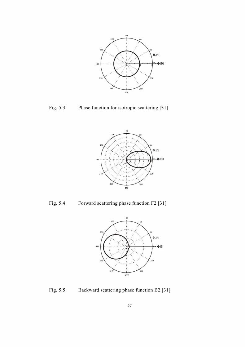
Fig. 5.3 Phase function for isotropic scattering [31]

Fig. 5.4 Forward scattering phase function F2 [31]

Fig. 5.5 Backward scattering phase function B2 [31]

57

5.2 FREEBOARD OF AN ATMOSPHERIC BUBBLING FLUIDIZED

BED COMBUSTOR PROBLEM

The physical situation under consideration is the freeboard section of

METU 0.3 MWt Atmospheric Bubbling Fluidized Bed Combustor (ABFBC).

The detailed description of the freeboard and properties of the participating

medium are given in the references [24, 26, 27, 28, 29, 32, and 33].

As the problems are set to be more realistic and closer to the real

engineering problems, the idealizations are lost and the approximate

methods generally result in larger errors. However, some idealizing

assumptions can still be made in most of the engineering systems. The

freeboard is treated as a 3-D rectangular enclosure containing grey,

absorbing, emitting, isotropically/anisotropically scattering medium with

uniform radiative properties. The flow chart of the MCM code for the

freeboard problem is given in Appendix Fig.A3.

5.2.1 Description of the Test Rig

The main body of the test rig is a modular combustor formed by five

modules of 1 m height with internal cross-section of 0.45 m x 0.45 m. The

first and the fifth modules refer to the bed and the cooler, respectively, and

the three modules in between are the freeboard modules.

Temperature profiles of the wall and medium are reported by Selçuk

[27], and given in Figure 5.6. There are two cooling surfaces of 0.35 m2 and

4.3 m2 in the bed and cooler modules as shown in Fig. 5.7, respectively.

58

Wall and Medium Temperature

0

100

200

300

400

500

600

700

800

900

1000

0 1 2 3 4 5

Height, z(m)

CO

OLE

R

BED

Tw T

empe

ratu

re (o C

) Tg

Polynomials for temperature profiles;

Tg=-5.2962 z4+43.956 z3-146.52 z2+240.79 z+ 748.6 [oC]

Tw=-11.164 z3+54.123 z2-109.95 z+938.8 [oC]

Fig. 5.6 Temperature profiles along the freeboard [27]

5.2.2 Approximation of the ABFBC Freeboard as a 3-D Radiation Problem

In order to apply the radiation models to the freeboard, it is required

to provide temperatures and radiative properties of the surfaces and the

medium. The freeboard section of the combustor is treated as 3-D enclosure

containing grey, absorbing, emitting and isotropically/anisotropically

scattering medium bounded by diffuse, grey/black walls. The cooler

boundary at the top, which consists of gas lanes and cooler tubes, is

represented by an equivalent grey surface. The boundary with the bed

section at the bottom is represented as a black surface. The physical system

and the treatment of the freeboard are schematically shown in Fig. 5.7.

59

Radiative properties of the particle laden combustion gases and

radiative properties and temperatures of the bounding surfaces are

summarized in Table 5.3. These data together with medium and sidewall

temperature profiles given in Fig.5.6 provide the input data supplied to the

radiation models.

Table 5.3 Radiative properties of the medium and the surfaces [27]

Gas absorption coefficient, κg (1/m) 0.43

Absorption coefficient of particle cloud, κp (1/m) 0.16

Scattering coefficient of particle cloud, σs (1/m) 0.45

Extinction coefficient of the particles, βp= κp+ σs (1/m) 0.61

Absorption coefficient of the medium, κ= κp+κg (1/m) 0.59

Extinction coefficient of the medium, β= κ+ σs (1/m) 1.04

Scattering albedo of the medium, ω= σs/ β 0.43

Emissivity of top surface, εtop 0.87

Emissivity of side surfaces, εw 0.33

Emissivity of bottom surface, εbottom 1.00

Temperature of top surface (oC), Ttop 549

Temperature of bottom surface (oC), Tbottom 873

60

Fig.

5.7

Tr

eatm

ent o

f fre

eboa

rd a

s a 3

-D e

nclo

sure

and

solu

tion

dom

ain

for M

onte

Car

lo M

etho

d [2

7]

61

CHAPTER 6

RESULTS AND DISCUSSION

The accuracy of the Monte Carlo method is examined by applying it

to the enclosure problems described in Chapter 5. Based on the results and

comparisons with the MOL of DOM solution of the same problems, it is

possible to comment on the accuracy and computational efficiency

properties of the MCM used for the problems under consideration.

In all cases, a computer, which has Intel Celeron 300 MHz processor and

double precision of a FORTRAN compiler, is used.

6.1 3-D CUBICAL ENCLOSURE PROBLEM CONTAINING

SCATTERING MEDIUM

In this part, the 3-D cubical enclosure problems, containing a

scattering medium, are investigated. The physical system is a uniform, grey,

purely scattering or absorbing, emitting and scattering medium bounded by

diffuse, grey walls. Isotropic and anisotropic conditions are analyzed.

Accuracy of MCM is tested by applying it to the two problems

described in Section 5.1 and comparing the predicted radiation variables

against MOL of DOM solutions by Ayrancı [24]. The effect of the total

number of photon histories used in MCM is investigated on the problem

containing purely, isotropically scattering medium with non-symmetric

62

boundary conditions. The parameters selected from this study are utilized in

the calculation of the same problem with anisotropy and in the second

problem with absorbing, emitting, and scattering problem.

In the cases that follow, the dimensionless radiative heat flux, Qi* as

given in Eq. (5.2) is used for comparative purposes with the available MOL of

DOM [24] solutions. The radiative heat flux along the i-coordinate, qi is

calculated by MCM as,

[ ]∑=

⋅⋅−=

M

1n n

ii A

swnlniq (6.1)

where, ni is the total number of incident photons on the surface or sub-

volume, nl is the number of leaving photons from the surface or sub-volume,

w is the photon energy, s is the direction cosine along the i-coordinate, Aiˆ n

is the surface area normal to the i-coordinate, and finally M is the total

number of photons emitted in the enclosure.

6.1.1 PURELY SCATTERING WITH NON-SYMMETRIC BOUNDARY

CONDITIONS

MCM solution of this problem is investigated by comparing its

predictions for radiative heat flux Qz* along the centerline of the enclosure

(Lo/2, Lo/2, z) with those of MOL of DOM solutions obtained by dividing the

enclosure into 25x25x25 sub-volumes using S10 order of approximation with

LSO (Level Symmetric Odd) quadrature and DSS012 spatial discretization

scheme [24].

The effect of grid spacing on the accuracy of MCM is investigated for

this problem. The comparisons between the predictions of heat fluxes along the

63

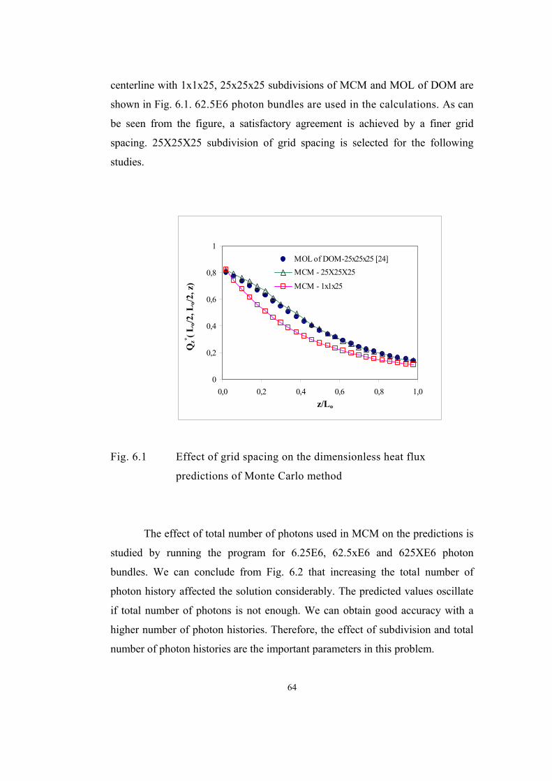
centerline with 1x1x25, 25x25x25 subdivisions of MCM and MOL of DOM are

shown in Fig. 6.1. 62.5E6 photon bundles are used in the calculations. As can

be seen from the figure, a satisfactory agreement is achieved by a finer grid

spacing. 25X25X25 subdivision of grid spacing is selected for the following

studies.

0

0,2

0,4

0,6

0,8

1

0,0 0,2 0,4 0,6 0,8 1,0

MOL of DOM-25x25x25 [24]MCM - 25X25X25

MCM - 1x1x25

Qz* ( L

o/2, L

o/2, z

)

o

Fig. 6.1 Effect of grid spacing on the

predictions of Monte Carlo m

The effect of total number of photons

studied by running the program for 6.25

bundles. We can conclude from Fig. 6.2 t

photon history affected the solution consider

if total number of photons is not enough. W

higher number of photon histories. Therefore

number of photon histories are the important

64

z/L

dimensionless heat flux

ethod

used in MCM on the predictions is

E6, 62.5xE6 and 625XE6 photon

hat increasing the total number of

ably. The predicted values oscillate

e can obtain good accuracy with a

, the effect of subdivision and total

parameters in this problem.

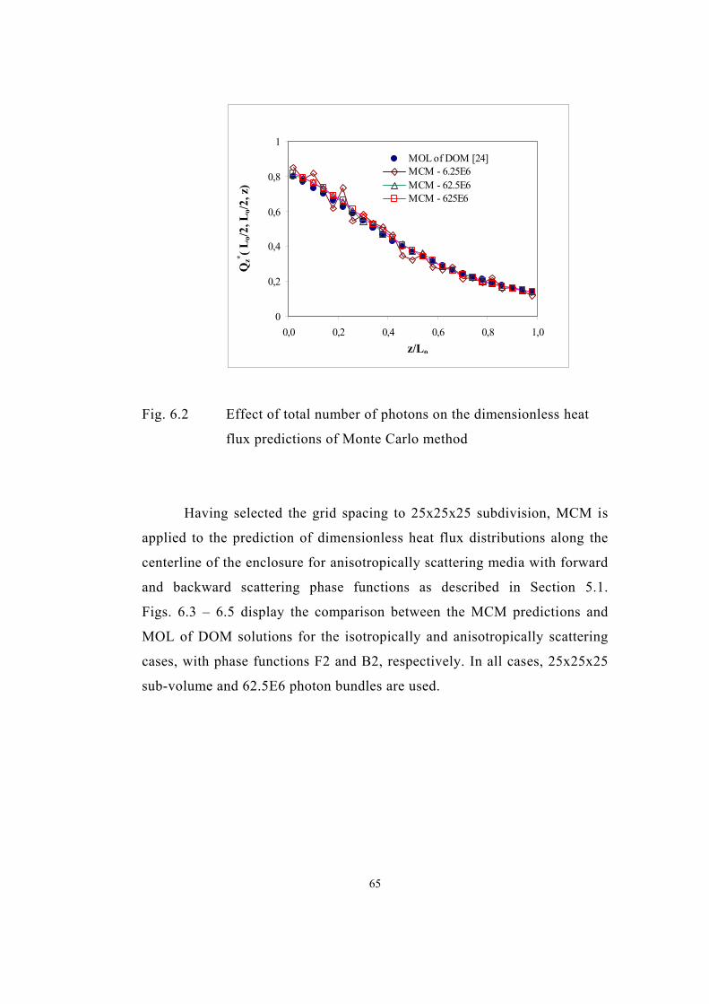
0

0,2

0,4

0,6

0,8

1

0,0 0,2 0,4 0,6 0,8 1,0

MOL of DOM [24]MCM - 6.25E6MCM - 62.5E6MCM - 625E6

Qz* ( L

o/2, L

o/2, z

)

Fig. 6.2 Effect of total number of pho

flux predictions of Monte Ca

Having selected the grid spacing to

applied to the prediction of dimensionless

centerline of the enclosure for anisotropica

and backward scattering phase function

Figs. 6.3 – 6.5 display the comparison be

MOL of DOM solutions for the isotropica

cases, with phase functions F2 and B2, re

sub-volume and 62.5E6 photon bundles are

65

z/Lo

tons on the dimensionless heat

rlo method

25x25x25 subdivision, MCM is

heat flux distributions along the

lly scattering media with forward

s as described in Section 5.1.

tween the MCM predictions and

lly and anisotropically scattering

spectively. In all cases, 25x25x25

used.

0

0,2

0,4

0,6

0,8

1

0,0 0,2 0,4 0,6 0,8 1,0

MOL of DOM - Isotropic [24]

MCM - Isotropic

Qz* ( L

o/2, L

o/2, z

)

Fig. 6.3 Comparison between pre

MOL of DOM for dimen

centerline for isotropicall

0

0,2

0,4

0,6

0,8

1

0,0 0,2 0,4

MOL

MCM

Qz* ( L

o/2, L

o/2, z

)



centerline for anisotropic

function F2 66

z/Lo

dictions of Monte Carlo method and

sionless heat flux profiles along the

y scattering medium

0,6 0,8 1,0

of DOM - F2 [24]

- F2

o
z/L


ally scattering medium with phase

0

0,2

0,4

0,6

0,8

1

0,0 0,2 0,4 0,6 0,8 1,0

MOL of DOM - B2 [24]MCM - B2

Qz* ( L

o/2, L

o/2, z

)



centerline for anisotropic

function B2

Table 6.1 Comparative testing

predictions of Monte Ca

various phase functions

Phase

function

*Average absolute

percentage error M

Isotropic** 1.47 F2** 6.57 B2** 6.69

*Absolute Percentage Error= (Q**62.5E6 photon

6

z/Lo



ally scattering medium with phase

between dimensionless heat flux

rlo method and MOL of DOM [24] for

aximum absolute

percentage error CPU Time, s

4.44 466.5

27.5 3262.6

22.2 887.5

) 100Q/Q *DOM of MOL

*DOM of MOL

*MCM ⋅−

bundles are used

7

As can be seen from the above figures, the MCM solution in isotropic

scattering medium agrees well with the MOL of DOM solutions, however there

are oscillations in the predictions of F2 and B2 anisotropic scatterings. The grid

spacing is insufficient to eliminate the oscillations. The grid spacing may be

increased in further studies.

6.1.2 ABSORBING, EMITTING, SCATTERING MEDIUM WITH

SYMMETRIC BOUNDARY CONDITIONS

The performance of MCM for this problem was investigated by

comparing its predictions for dimensionless radiative heat flux Qz* along the

centerline of a wall (x, Lo/2, Lo) with those of MOL of DOM [24] obtained by

dividing the enclosure into 25x25x25 sub-volumes, DSS012 scheme, S10 order of

approximation. In all cases, 25x25x25 sub-volume and 62.5E6 photon

bundles are used. Figures 6.6-6.8 illustrate the heat flux predictions of MCM

and MOL of DOM for various phase functions.

0

0,2

0,4

0,6

0,8

1

0,0 0,2 0,4 0,6 0,8 1,0

MOL of DOM - Isotropic [24]

MCM - Isotropic

Qz* (x

, Lo/2

, Lo )

x/Lo

Fig. 6.6 Comparison between predictions of Monte Carlo method and


x-axis for isotropically scattering medium

68

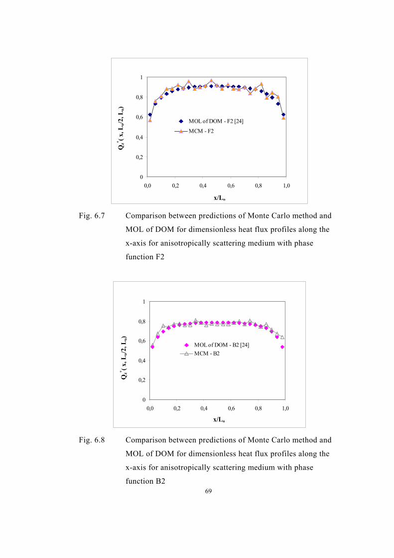
0

0,2

0,4

0,6

0,8

1

0,0 0,2 0,4 0,6 0,8 1,0

MOL of DOM - F2 [24]

MCM - F2

Qz* ( x

, Lo/2

, Lo)



x-axis for anisotropically

function F2

0

0,2

0,4

0,6

0,8

1

0,0 0,2 0,4

MOL oMCM

Qz* ( x

, Lo/2

, Lo)



x-axis for anisotropically

function B2 69

x/Lo



scattering medium with phase

0,6 0,8 1,0

f DOM - B2 [24]- B2

x/Lo



scattering medium with phase

The differences between the MCM and MOL of DOM are given in

Table 6.2. As can be seen from the figures and table, MCM predictions are

in reasonable agreement with those of MOL of DOM for isotropic scattering.

The grid spacing or the total number of photons emitted from the

enclosure is insufficient to eliminate the oscillations in anisotropic scattering.

Table 6.2 Comparative testing between dimensionless heat flux

predictions of Monte Carlo method and MOL of DOM [24] for

various phase functions

Phase

function

Average absolute

percentage error* Maximum absolute

percentage error CPU Time, s

Isotropic** 0.66 13.64 2742.6

F2** 1.82 13.94 13374.2

B2** 1.91 18.38 9155.5

*Absolute Percentage Error= ( ) 100Q/QQ *

DOM of MOL*

DOM of MOL*

MCM ⋅−

**62.5E6 photon bundles are used

6.2 FREEBOARD OF AN ATMOSPHERIC BUBBLING FLUIDIZED

BED COMBUSTOR

The freeboard section of the 0.3 MWt ABFBC is treated as a

rectangular enclosure with diffuse, grey walls containing an absorbing,

emitting, isotropically scattering medium. The predictive accuracy of MCM

is assessed by applying it to the prediction of incident radiative fluxes on

70

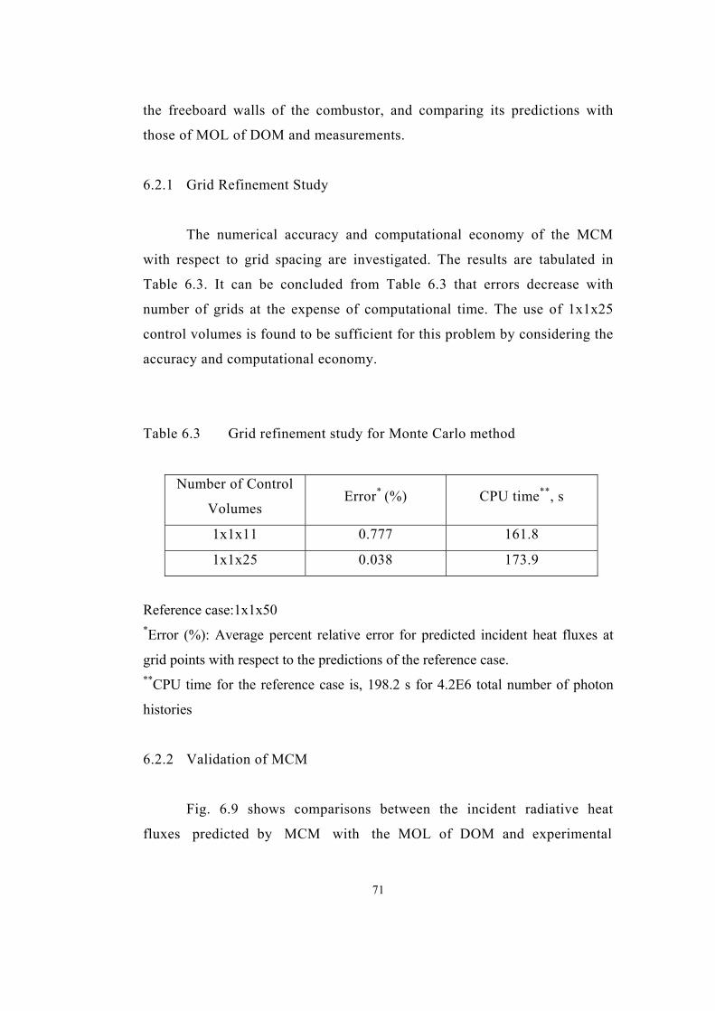
the freeboard walls of the combustor, and comparing its predictions with

those of MOL of DOM and measurements.

6.2.1 Grid Refinement Study

The numerical accuracy and computational economy of the MCM

with respect to grid spacing are investigated. The results are tabulated in

Table 6.3. It can be concluded from Table 6.3 that errors decrease with

number of grids at the expense of computational time. The use of 1x1x25

control volumes is found to be sufficient for this problem by considering the

accuracy and computational economy.

Table 6.3 Grid refinement study for Monte Carlo method

Number of Control

Volumes Error* (%) CPU time**, s

1x1x11 0.777 161.8

1x1x25 0.038 173.9

Reference case:1x1x50 *Error (%): Average percent relative error for predicted incident heat fluxes at

grid points with respect to the predictions of the reference case. **CPU time for the reference case is, 198.2 s for 4.2E6 total number of photon

histories

6.2.2 Validation of MCM

Fig. 6.9 shows comparisons between the incident radiative heat

fluxes predicted by MCM with the MOL of DOM and experimental

71

measurements. As can be seen from the figure, the incident flux decreases

from the bed surface towards the cooler ones. The predictions are in good

agreement with the MOL of DOM and the measurements [27].

0

20

40

60

80

100

120

0 1 2 3 4 5

MCM

Measurements [27]

MOL of DOM [27]

Inci

dent

Rad

. Hea

t Flu

x (k

W/m

2 )

CO

OLE

R

BED

Height, z (m)

Fig. 6.9 Incident radiative heat fluxes on freeboard wall

A heat flux transducer is used to measure the incident radiative heat

fluxes on the walls of the freeboard [27]. The measurements are taken

during the steady-state operation of the ABFBC. The experimental

measurements are given in detail in the references [26, 27, 28, and 29]. The

predicted and measured values are a little different at the ports adjacent to

the bed and cooler surfaces. Because, the cooling tubes at the bed and cooler

surfaces affected the radiometer probe measurements adjacent to the top and

bottom surfaces.

72

For comparative testing purposes, the values of the predicted fluxes

are compared with the measurements at discrete points. Table 6.4 illustrates

the relative percentage errors in the fluxes predicted by both methods. As

can be seen from the table, percentage errors are very close to each other.

Table 6.4 Incident radiative heat fluxes on freeboard wall

Predictions(kw/m2) Relative Error (%)

Height (m)

Experimental MOL of DOM [27] Monte Carlo* MOL of DOM

[27] Monte Carlo*

1.23 108,9 99 98,9 -9,1 -9,0

1.83 96,4 98,8 99,5 2,5 3,0

2.91 90,2 90,1 90,9 -0,1 0,5

3.44 71,5 78 78,6 9,1 9,7

4.19 28 47,3 46,8 68,9 67,2

(kw/m2) [27]

*1x1x25 subvolume is used in Monte Carlo Solution * CPU time for Monte Carlo Solution is, 173.9 s for 4.2E6 total number

of photon histories

6.2.3 Parametric studies

Sensitivity of the incident heat flux to the presence of particles is

analyzed by comparing the predictions of MCM with and without particles (Fig.

6.10). As it can be seen from the figure, the effect of particles on the

predicted heat fluxes is not considerable.

73

0

20

40

60

80

100

120

0 1 2 3 4 5

qas+particle

only gas

Inci

dent

Rad

. Hea

t Flu

x (k

W/m

2 )

CO

OLE

R

BED

Height, z (m)

Fig. 6.10 Sensitivity of radiative heat flux to the presence of particles

CPU time for gas+particle and only gas cases are given at Table 6.5

below for 11E6 total number of photon histories used in the calculations.

The effects of particle load and anisotropic scattering on the incident

heat fluxes are examined. The real case analyzed previously with isotropic

scattering assumption is taken as the basis, and three different cases are

generated by increasing the particle load and/or by incorporating strong

anisotropy into the problem. The effect of anisotropy is analyzed by

utilizing linear anisotropy assumption,

( ) θ′+=′⋅+=′⋅Φ cosA1ssA1ss 11 (6.2)

where it is assumed that the polar angle θ’ is measured from an axis pointing into

the . As 1 is equal to 1 for the strong forward scattering case. In addition to the

anisotropic case, a high particle load case is also investigated. The particle load

74

is increased 1000 times which leads to, κ ≈ 160 (absorption coefficient of the

medium) and σs ≈ 450 (scattering coefficient of the medium). CPU times are

given in Table 6.5 for 220E6 total number of photon histories.

0

20

40

60

80

100

120

0 1 2 3 4 5

baseanisotropichigh particle loadhigh particle load+anisotropic

Inci

dent

Rad

. Hea

t Flu

x (k

W/m

2 )

CO

OLE

R

BED

Height, z (m)

Fig.6.11 Effect of high particle load and anisotropy on incident

radiative flux

Table 6.5 CPU times of parametric studies

Gas +

particle

Only

gas Base Anisotropic

High particle

load

High particle load

+ anisotropic

CPU

Time, s 210.4 225.2 4504.7 4300.8 3199.9 2992.5

75

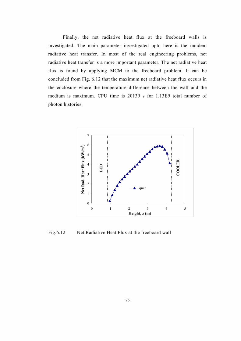
Finally, the net radiative heat flux at the freeboard walls is

investigated. The main parameter investigated upto here is the incident

radiative heat transfer. In most of the real engineering problems, net

radiative heat transfer is a more important parameter. The net radiative heat

flux is found by applying MCM to the freeboard problem. It can be

concluded from Fig. 6.12 that the maximum net radiative heat flux occurs in

the enclosure where the temperature difference between the wall and the

medium is maximum. CPU time is 20139 s for 1.13E9 total number of

photon histories.

0

1

2

3

4

5

6

7

0 1 2 3 4 5

qnet

Net

Rad

. Hea

t Flu

x (k

W/m

2 )

CO

OLE

R

BED

Height, z (m)

Fig.6.12 Net Radiative Heat Flux at the freeboard wall

76

CHAPTER 7

CONCLUSIONS AND FUTURE WORK

7.1 CONCLUSIONS

The accuracy of Monte Carlo method is re-examined by applying it

to three-dimensional radiative heat transfer problems with participating

media and comparing its predictions against measurements and/or

benchmark solutions reported in the literature.

The predictive accuracy of the method is examined for:

• Cubical enclosure problems containing purely scattering and absorbing,

emitting scattering media with isotropic and anisotropic scattering

properties by validating the solutions against MOL of DOM solutions

available in the literature,

and

• A physical problem, which is the freeboard of pilot-scale atmospheric,

bubbling fluidized bed combustor by comparing its predictions with

those of the MOL of DOM solutions and measurements.

The following conclusions have been reached on the basis of

comparative testing procedure:

77

• MCM is predicting radiative heat transfer accurately in a cubical

enclosure containing purely scattering medium. On the contrary, MCM

results are oscillating through the MOL of DOM results for anisotropic

cases. The grid spacing, and total number of photon emitted from the

enclosure can be further investigated for anisotropic cases.

• When the results are considered, it could be concluded that the solution

accuracy of the MCM is sufficient to predict radiative heat flux for

three-dimensional problems with isotropically scattering media. The

solutions of MCM for anisotropic media show some oscillation, but

oscillations become smaller when sufficiently high numbers of total

histories are used in the solution.

• MCM reproduces the measured incident radiative heat fluxes

reasonably well for the freeboard problem.

• MCM is as accurate as the MOL of DOM.

Some parametric studies are also considered. Particle load effect and

anisotropy on the predicted radiative fluxes are as follows,

• Presence of particles in the participating media does not affect the

magnitude of predicted incident heat fluxes.

• Increasing the particle load an order of magnitude leads to significant

rise in incident radiative fluxes at the wall.

Effect of anisotropy on the incident radiative heat fluxes on the side walls is

negligible for the situation under consideration.

78

7.2 FUTURE WORK

Further developments can be utilized for the Monte Carlo method so

that the problems at hand can be extended to involve nonhomogeneous and

nongrey media.

The Monte Carlo method can efficiently be utilized in complete

combustion models considering the increase in capability of computers and

with the use of parallel processing.

79

REFERENCES

1. J.R. Howell and M. Perlmutter, 1964, “Monte Carlo Solution of

Thermal Transfer Through Radiant Media Between Gray Walls”,

Journal of Heat Transfer, vol. 86 (1), pp. 116-122

2. C. M. Usiskin and E.M. Sparrow, 1960, “Thermal radiation between

parallel plates separated by an absorbing-emitting-non-isothermal gas”,

Intern. J. Heat and Mass Transfer 1, 28

3. R. G. Deissler, 1964, “Diffusion approximation for thermal radiation

in gases with jump boundary condition”, J. Heat Transfer 86, 240

4. J.R. Howell and M. Perlmutter, 1964, “Radiant Transfer Through a

Gray Gas Between Concentric Cylinders Using Monte Carlo”, Journal

of Heat Transfer, vol. 86 (2), pp. 169-179

5. J.R. Howell, 1968, “Application of Monte Carlo to Heat Transfer

Problems”, Advances in Heat Transfer, vol. 5, pp.1-55, Academic

Press, New York

6. A. Hajii Sheikh, 1998, “Monte Carlo Methods”, in: Handbook of

Numerical Heat Transfer edited by W.J. Minkowycz et al, pp.673-723,

Wiley, New York

7. A. Mochida, K. Kudo, Y. Mizutani, M. Hattori, Y. Nakamura, 1997,

“Transient Heat Transfer Analysis in Vacuum Furnaces Heated By

80

Radiant Tube Burners”, Energy Convers. Mgmt, vol.38 No10-13,

pp.1169-1176

8. H. Taniguchi, O. Toshiaki, M. Iwata, N. Arai, K. Hiraga, S.

Yamaguchi, 2002, “Numerical Study of Radiation-Convection Heat

Transfer”, Heat Transfer-Asian Research, vol. 31(5), pp. 391-407

9. L. H. Liu, H. P. Tan, Q. Z. Yu, 2003, “Temperature Distributions in an

Absorbing–Emitting–Scattering Semitransparent Slab with Variable

Spatial Refractive Index”, International Journal of Heat and Mass

Transfer, pp.2917-2920

10. P.B. Abdallah, V. Le Dez, 2000, “Thermal field inside an absorbing,

emitting, semi-transparent slab at radiative equilibrium with variable

spatial refractive index”, J. Quant. Spectrosc. Radiat. Transfer, vol 65,

pp. 595–608

11. L. H. Liu, X. Xu, 2003, “Monte Carlo Ray-Tracing simulation for

Radiative Heat Transfer in Turbulent Fluctuation Media under the

Optically Thin Fluctuation Approximation”, Journal of Quantitative

Spectroscopy and Radiative Transfer, pp. 1-7

12. R. Vaillon, B.T. Wong, P. Mengüç, 2003, “ Polarized Radiative

Transfer in a Particle-laden Semi-transparent Medium via a Vector

Monte Carlo Method”, Proceedings of Eurotherm 73 on

Computational Thermal Radiation in Participating Media

13. R. Couqard, D. Baillis, D. Quenard, 2003, “Radiative Properties of

Semi-transparent Spherical Particle Beds, Proceedings of Eurotherm

73 on Computational Thermal Radiation in Participating Media

81

14. A. Snergiev, 2003, “ Monte Carlo Modelling of Radiative Transfer in

Unconfined Buoyant Turbulent Diffusion Flames”, Proceedings of

Eurotherm 73 on Computational Thermal Radiation in Participating

Media

15. B.T. Wong, P. Mengüç, 2003, “Monte Carlo Methods in Radiative

Transfer and Electron-beam Processing”, Proceedings of Eurotherm 73

on Computational Thermal Radiation in Participating Media

16. Q. Yu, L. Liu, Y. Pan, D. Zhang, J. Ji, and H. Ta, 1999, “Monte Carlo

Method for Simulating the Radiative Characteristic of an Anisotropic

Medium”, Journal of Heat Transfer Asian Research, vol. 28 (3), pp.

201-210

17. J.G.Marakis, C.Papapavlou, E.Kakara, 2000, “A parametric Study of

Radiative Heat Transfer in Pulverised Coal Furnace”, International

Journal of Heat and MassTransfer, vol. 43, pp. 2961-2971

18. W. Chai, 1997, “Radiative Heat Transfer Model in Arbitrary

Enclosures by Ray-Tracing”, Proceedings of the 2nd International

Symposium on Radiation Transfer, edited by P. Mengüç, Begell House,

New York, pp. 55-73

19. H. Ertürk, F. Arınç, N. Selçuk, 1997, “Accuracy of Monte Carlo

Method Re-examined on a Box-shaped Furnace Problem”, Proceedings

of the 2nd International Symposium on Radiation Transfer, edited by P.

Mengüç, Begell House, New York, pp. 85-95

20. H. Ertürk, 1997, “Mathematical Modeling of Radiative Heat Transfer

in Participating Meida”, Metu, Msc. Thesis

82

21. N. Selçuk, 1981, “Fırınlardaki Işınım Isı Transferinin Tam Çözümü ve

Akı Yöntemlerinin İrdelenmesi”, ODTÜ, Doçentlik Tezi

22. N. Selçuk, 1985, “Exact Solutions for Radiative Heat Transfer in Box-

Shaped Furnaces”, ASME Journal of Heat Transfer, vol. 107, pp.648-

655

23. T.W. Tong and R.D. Skocypec, 1992, “Summary on Comparison of

Radiative Heat Transfer Solutions for a Specified Problem”, ASME

HTD-Developments in Radiative Heat Transfer, Vol. 203, pp.253-258

24. I. Ayrancı, 2001, “The Method of Lines Solution of Discrete Ordinates

Method for Radiative Heat Transfer in 3-D Rectangular Enclosures

Containing Scattering Media”, Metu, Msc. Thesis

25. S. H. Kim, K. Y. Huh, 2000, “A new Angular Discretization Scheme

of the Finite Volume Method for 3-D Radiative Heat Transfer in

Absorbing, Emitting and Anisotropically Scattering Media”, Int. J.

Heat Mass Transfer, Vol. 43, pp. 1233-1242

26. A. Batu, N. Selçuk, 2002, “Modeling of Radiative Heat Transfer in the

Freeboard of a Fluidized Bed Combustor Using the Zone Method of

Analysis”, Turkish J. Eng. Env. Sci., vol.26, pp. 49-58

27. N. Selçuk, A. Batu, I. Ayrancı, 2001, “Performance of Method of

Lines Solution of Discrete Ordinates Method in the Freeboard of a

Bubbling Fludized Bed Combustor”, Proceedings of the 3rd

International Symposium on Radiation Transfer, edited by P. Mengüç

and N. Selçuk, Begell House, New York, pp. 527-538

83

28. M. Kozan, 1999, “Investigation of Radiative Heat Transfer in

Freeboard of a 0.3 MWt AFBC Test Rig”, METU, Msc. Thesis

29. M. Kozan, N. Selçuk, 2000, “Investigation of Radiative Heat Transfer

in Freeboard of a 0.3 MWt AFBC Test Rig”, Combust. Sci. Tech. Vol.

153, pp 113-126

30. M.F. Modest, 1993, Radiative Heat Transfer, McGraw Hill, New York

31. T.-K. Kim and H Lee, 1988, “Effect of Anisotropic Scattering on

Radiative Heat Transfer in Two-dimensional Rectangular Enclosures”,

Int. J. of Heat Transfer, Vol.31(8), pp.1711-1721

32. N. Selçuk, E. Değirmenci and Y. Göğebakan, 2000, “Assessment of

Catalyst Deactivation Model for Sulfur Rtention in Fluidized Bed

Combustors”, Combust. Sci. Tech., Vol. 153, pp 95-111

33. E. Değirmenci, 2000, “Dynamic Simulation of Fludized Bed

Combustors”, METU, PhD. Thesis

34. R. Siegel and J.R. Howell, 1992, “Thermal Radiation Heat Transfer”,

3rd ed., Hemisphere, Washington

35. F.P. Incropera, and D.P. DeWitt, 1994, “Fundamentals of Heat and

Mass Transfer”, 4th ed., John Wiley and Sons, New York

84

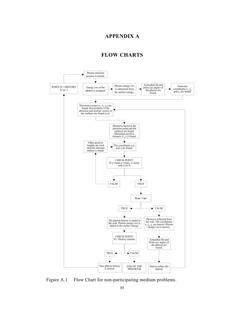
APPENDIX A

FLOW CHARTS

Energy (w) of thephoton is assigned.

Azimuthal (θ) andpolar (ψ) angles of

the photon arefound.

Emissioncoordinates xe ,yeand ze are found.

Photon energy (w)is subtracted fromthe surface energy.

Direction cosines (si, sj, sk) arefound. Dot products of the

direction and normal vectors ofthe surfaces are found (s.n).

Photon emissionprocess is started.

Distances between theemission point and the

surfaces are found.Minumum positive

distance (Lw) is found.

The coordinates x,y,and z are found.

CHECK POINT!If x<xmax,y<ymax, z<zmax

and (s.n)<0

The photon history is ended atthe wall. Photon energy (w) isadded to the surface energy.

New photon historyis started.

TRUE FALSE

Photon is reflected fromthe wall. The coordinatesxe,ye,ze are known. Photon

energy (w) is known.

Start to reflect thephoton

FALSE

CHECK POINT!N<=History number

FALSETRUE

END OF THEPROGRAM

Reps<=eps

TRUE

WHEN N<=HISTORYN=N+1

Other positivelengths are trieduntil the directedsurface is found.

Azimuthal (θ) andPolar (ψ) angles of


Figure A.1 Flow Chart for non-participating medium problems.

85





Photon energy (w)is subtracted fromthe surface or sub-

volume energy.









and (s.n)<0

The photon history isended at the wall.

Photon energy (w) isadded to the surface

energy.


TRUE FALSE

Photon is reflected fromthe wall. The coordinates

xe,ye,ze are known.Photon energy (w) is

known.


FALSE


FALSETRUE

END OF THEPROGRAM

Reps<=eps

TRUE





Absorption (Lκ)and scattering (Lσ)

mean free pathlengths are found.

Lw, Lκ and Lσ arecompared.

If Lw is thesmallest, photonis directed to theenclosure wall

If Lκ is thesmallest, photonis absorbed inthe medium

If Lσ is thesmallest, photonis scattered in the

medium

The photon history is ended inthe medium. Photon energy

(w) is added to the sub-volume energy.


New photonhistory is started.

FALSETRUE

END OF THEPROGRAM

Lκ (Lκ=Lκ-Lw), andLσ (Lσ=Lσ-Lw) are

updated.

The coordinatesxe,ye,ze are known.

Photon energy (w) isknown.

Azimuthal (θ) andPolar (ψ) anglesof the photon are

found.

Lκ (Lκ=Lκ-Lσ), andLσ are updated.

Start to scatter thephoton

Figure A.2 Flow Chart for cubical enclosure problems

86













and (s.n)<0

The photon history isended at the wall.

Photon energy (w) isadded to the incident

surface energy.


TRUE FALSE

Photon is reflected fromthe wall. The coordinates

xe,ye,ze are known.Photon energy (w) isadded to the incident

surface energy.


FALSE


FALSETRUE

END OF THEPROGRAM

Reps<=eps

TRUE





Absorption (Lκ)and scattering (Lσ)

mean free pathlengths are found.

Lw, Lκ and Lσ arecompared.

If Lw is thesmallest, photonis directed to theenclosure wall

If Lκ is thesmallest, photonis absorbed inthe medium

If Lσ is thesmallest, photonis scattered in the

medium

The photon history is ended inthe medium. Photon energy(w) is added to the incident

sub-volume energy.


New photonhistory is started.

FALSETRUE

END OF THEPROGRAM

Lκ (Lκ=Lκ-Lw), andLσ (Lσ=Lσ-Lw) are

updated.

The coordinatesxe,ye,ze are known.

Azimuthal (θ) andPolar (ψ) anglesof the photon are

found.

Lκ (Lκ=Lκ-Lσ), andLσ are updated.

Start to scatter thephoton

Photon energy (w) is added tothe incident sub-volume

energy.

Figure A.3 Flow Chart for freeboard problems

87

monte carlo solution of a radiative heat transfer...

Documents