molecular dynamics of apo-adenylate kinase: a … 110...molecular dynamics of apo-adenylate kinase:...

Molecular Dynamics of Apo-Adenylate Kinase: A Distance Replica Exchange Method forthe Free Energy of Conformational Fluctuations

Hongfeng Lou and Robert I. Cukier*Department of Chemistry and the QuantitatiVe Biology Modeling InitiatiVe, Michigan State UniVersity,East Lansing, Michigan 48824-1322

ReceiVed: July 8, 2006; In Final Form: September 8, 2006

A large domain motion in adenylate kinase fromE. coli (AKE) is studied with molecular dynamics. AKEundergoes a large-scale rearrangement of its lid and AMP-binding domains when the open form closes overits substrates, AMP, and Mg2+-ATP, whereby the AMP-binding and lid domains come closer to the core.The third domain, the core, is relatively stable during this motion. A reaction coordinate that monitors thedistance between the AMP-binding and core domains is selected to be able to compare with the results ofenergy transfer experiments. Sampling along this reaction coordinate is carried out by using a distance replicaexchange method (DREM), where systems that differ by a restraint potential enforcing different reactioncoordinate values are independently simulated with periodic attempts at exchange of these systems. Severalmethods are used to study the efficiency and convergence properties of the DREM simulation and comparedwith an analogous non-DREM simulation. The DREM greatly accelerates the rate and extent of configurationalsampling and leads to equilibrium sampling as measured by monitoring collective modes obtained from aprincipal coordinate analysis. The potential of mean force along the reaction coordinate reveals a rather flatregion for distances from the open to a relatively closed AKE conformation. The potential of mean force forsmaller distances has a distinct minimum that is quite close to that found in the closed form X-ray structure.In concert with a decrease in the reaction coordinate distance (AMP-binding-to-core distance) the lid-to-coredistance of AKE also decreases. Therefore, apo AKE can fluctuate from its open form to conformations thatare quite similar to its closed form X-ray structure, even in the absence of its substrates.

1. Introduction

Adenylate kinase (AK) catalyzes the reversible transforma-tion.

There are three domains in AKs: core, lid, and AMP-binding(Amp-bd). AKs are thought to be in an open form in the absenceof substrates and, when Mg2+-ATP and AMP are present, thelid and Amp-bd domains undergo major conformational rear-rangements, resulting in the closed form ternary complex.1

Extensive kinetic studies of rabbit AK (with a shorter lid domainthan in AKE) indicate that it occurs by an isorandom Bi Bimechanism, in which the two substrates can bind in randomorder to one isoform while the two products bind in randomorder to another isoform of the enzyme.2 These kinetics suggestthat apo-AKE can exist in at least two conformations, with oneform binding Mg2+-ATP and AMP and the other Mg2+-ADPand ADP.2 Other experiments3,4 suggest that each of thesesubensembles encompasses of a variety of conformers. NMRstudies also support the existence of a conformational ensemblefor the apo enzyme.5 The importance of domain conformationalchanges has been emphasized by recent experiments showingthat they, versus the chemical, phosphoryl transfer step, are ratelimiting in AKE and can rationalize differences in activity

between mesophiles and thermophiles.6 Crystallography1 andtime-resolved dynamic nonradiative excitation energy transferexperiments7 show that binding AMP is associated with an initialconformational change. Binding of the next substrate, usuallymodeled with a binary substrate, mimics AP5A (ATP and AMPlinked by a fifth phosphate group), resulting in the formationof the closed, catalytically competent form. The transition fromapo (open) to closed forms involves rearrangements withsignificant lid and Amp-bd domain motion to close theinterdomain cleft.8 The energy transfer studies of domain closurein AKE were carried out by labeling appropriate pairs ofresidues, Ala55, a residue in the Amp-bd domain and Val169,which is just below the lid, and distance distributions that reflectthe conformational space exploration were obtained. The apo-enzyme has a broad distance distribution, with a mean and widtharound 30 Å. The width of this distribution indicates that apo-AKE samples a very large conformational ensemble in solution.

Two extremes of a ligand/substrate binding mechanism canbe envisaged. The ligand could bind to the apo form and inducethe required conformational changes (“induced fit”) or it couldselect from preexisting protein conformations that are already“predisposed” to the ligand (“conformational selection”). Kosh-land9 refined Fisher’s lock and key hypothesis into the conceptof induced fit, which he defined as a close fit between the proteinand ligand that occurs only after conformational changes areinduced by the ligand.9 On the other hand, it may be that proteinswere designed to sample conformations that are predisposed tocapture substrates, to yield the final substrate-bound structure.10-13

There is evidence for this latter view in proteins such as* Corresponding author. E-mail: [email protected]. Telephone: 517-

355-9715, extension 263. Fax: 517-353-1793.

SCHEME 1

24121J. Phys. Chem. B2006,110,24121-24137

10.1021/jp064303c CCC: $33.50 © 2006 American Chemical SocietyPublished on Web 11/07/2006

staphylococcal nuclease,14,15calbindin,16 adenylate kinase3,4 andcalmodulin,17 and cyclophilin A.13 The data noted above on largedomain motions in AKE provides a good test system to beginan exploration of these two views of ligand binding. But, ifprotein molecular dynamics (MD) with explicit solvent is runon the current practical time scale of nanoseconds, simulationsof the apo form will tend to stay around that minimum, as wehave found in a previous AKE study.18 The large rearrangementsrequired to go from the apo to more closed forms cannot beaccessed on an MD time scale. That has stimulated a numberof studies of adenylate kinase based on the elastic network model(ENM), which is a reduced description relative to atomistic MDand MC approaches,19-21 Temiz et al.19 studied the open andclosed forms with the ENM, Miyashita et al.20 connect the twoforms using a small set of normal modes that are locally adjustedalong a path between the two, and Maragakis and Karplus21

use a minimum energy path method to span the two extremes.The generic sampling problem, which is due to the complexity

of the protein’s energy landscape, with barriers large comparedwith the thermal energy separating stable states, is a majorconcern in MD and Monte Carlo (MC) simulations. A numberof methods, such as multicanonical ensemble,22,23 simulatedtempering,24,25 and the replica exchange method (REM),26-29

were designed to address this issue. The REM was proposed26,30

in the context of Ising spin glasses31 and introduced toproteinlike systems by Sugita and Okamoto.27 The originalversions of the REM used temperature (TREM), and morerecently, a Hamiltonian REM (HREM) was introduced.32 Thesemethods all contain two elements: (1) Multiple copies ofconfigurations are run independently by MD or MC withdifferent temperatures and/or Hamiltonians. (2) Two neighborsin the sense of temperature and/or Hamiltonian are exchanged,according to the Metropolis-Hastings algorithm.33 Differentfrom multicanonical ensemble and simulated tempering meth-ods, the REM does not need to perform trial runs to determinea weight (density of states), as is required in the multicanonicalensemble23 and simulated tempering methods.24,25In the TREM,the low-indexed system (usually low temperature) borrows fastequilibration properties from high-indexed systems. That pro-vides a doorway for the low-indexed system to overcome energybarriers and thus improve the sampling.34 However, the numberof replicas needed in the TREM is unfortunately proportionalto the square root of the number of degrees of freedom of thesystem of interest.32

Fukunishi et al.32 proposed the HREM, in which the potentialfunction in different Hamiltonians differs by a small subset ofthe total number of degrees of freedom required to characterizethe system. By doing this, one hopes that the number of replicasneeded will be reduced. One way to change the Hamiltonianthat is well suited to a study where a reaction coordinate isintroduced is to integrate the umbrella sampling method33 withthe HREM. Namely, one creates different systems by addingdifferent umbrella window potential functions to the originalsystem that serve to restrain the systems to different values ofthe reaction coordinate. We will refer to this specialization ofHREM as the distance REM (DREM). This idea was proposedby Sugita and co-workers in the context of a multidimensionaltemperature and distance replica exchange method and appliedto the alanine trimer.35

In this work, we use the DREM to investigate if apo-AKEcan reach conformations that are similar to those found in thesubstrate bound structures. Harmonic potentials are used as thewindow potentials along a reaction coordinate, which is thedistance between the mass centers of residues Ala 55 and Val

169, to match the residues used in the energy transfer experi-ments.7 The potential of mean force along this reactioncoordinate over a range of approximately 35 Å is obtained withuse of the DREM. The large range of the reaction coordinatespans the open and closed X-ray structure values. Because thisapplication of the DREM is designed to probe a very largeconformational change in a protein with an explicit solventsimulation, a careful study of the quality of the simulation andits advantages over conventional umbrella sampling (no DREM)is carried out. We find that the DREM does provide enhancedsampling versus no DREM, as measured by improvements inthe speed of decay of time correlation functions and the extentof conformational space exploration. The DREM provides asufficient enhancement in sampling that, over the simulationlength, convergence with respect to motions that reflect thelarge-scale movement of AKE is achieved.

In Section 2 the DREM is introduced and details of itsapplication to the AKE simulation are provided, along withvarious methods to investigate its convergence and enhancedsampling quality. Section 3 first addresses the validation of theacceptance ratio in the DREM exchanges and then studies theconvergence to equilibrium of the sampling and measures ofthe DREM sampling improvement versus no-DREM. Thepotential of mean force is then presented along with relatedquantities that provide a picture of the motion of AKE in itsconfiguration space. Our conclusions are presented in Section4.

2. Methodology

Distance Replica Exchange Method.The temperature REM(TREM) constructs independent copies of a system that differby their temperature. The REM concept can be generalized toa Hamiltonian REM,32 where the systems differ by theirHamiltonian (in practice, in their potential energy function). Asa matter of terminology, we shall refer to these differentHamiltonians assystems(versus replicas) because replicaconnotes a copy of an item. The term replicas will be reservedfor the configurations that are present on any particular MDstep. It is perhaps useful to take an operational point of viewand consider that each processor on a computer is assigned aparticular system (Hamiltonian) and different replicas (configu-rations) can visit that particular processor (system). In our MDprogram, CUKMODY, however, a given replica is maintainedon a particular processor and the systems (the window functionparameters) move onto and out of that processor.

If the desire is to enhance the sampling along a chosenreaction coordinate, then systems that differ by a windowpotential to maintain a desired distance can be introduced togive a distance REM (DREM). Thus, we add a window potentialWi(r ) (i ) 1, 2, ...,N) to the original HamiltonianH0(X) wherer ) f(X) is any reaction coordinate dependent onX, theconfiguration point, so thatHi(X) ) H0(X) + Wi(r ). As in theHREM,32 appeal to the detailed balance condition

where R(X iX j f X jX i) is the acceptance probability thatconfigurationX i in the ith system exchanges with configurationX j in the jth system andPi(X) is the Boltzmann distribution attemperatureT ) 1/kBâ for the ith system provides a rule forthe exchange between two systems. In our case of a one-dimensional distance reaction coordinate,r, the ith windowfunction is chosen as a harmonic restraintWi(r) ) ki(r - r0

i )2

R(X iX j f X jX i)Pi(X i)Pj(X j) ) R(X jX i f X iX j)Pi(X j)Pj(X i)

(2.1)

24122 J. Phys. Chem. B, Vol. 110, No. 47, 2006 Lou and Cukier

with ki and r0i the force constant and equilibrium distance,

respectively. The acceptance probability that follows from eq2.1 and the harmonic window potential is

where

In the case of the same force constant for all windows, eq 2.2bsimplifies to

Between the attempted exchange steps, conventional MDsimulations are performed for the different systems. In theTREM (DREM), the exchanges may be thought of as config-uration or temperature (window) exchanges. From the compu-tational perspective, it is a great advantage of the DREM thatonly the force constant and equilibrium distance parameters needbe exchanged (eq 2.2b) or just the equilibrium distanceparameters (eq 2.2c). The exchanges are attempted betweenneighboring windows because, for the method to be effective,the overlap between the windows’ probability distributions needsto be adequate. In contrast with the TREM (unless ensembleaverages at higher temperatures than the “normal” one are ofinterest), the information from all the windows is used directlybecause it will ultimately provide the potential of mean forcealong the reaction coordinate. The details of the DREMapplication to AKE are given below.

Molecular Dynamics Simulations.The CUKMODY proteinmolecular dynamics code, which uses the GROMOS9636 forcefield, was modified to incorporate the DREM. The systems arerun independently on different nodes of a Linux cluster computerand, when exchanges are attempted, information is passed usingthe message passing interface technique implemented as MPICH.

Four simulations were performed that we shall refer to asDREMA, DREMP, DREMB, and NoDREM. The simulationswere run at 303 K under fixed number, volume, and temperature(NVT) conditions.37 In the DREMA and DREMB, different forceconstants are used, and the window function parameters arecollected in Table 1. The parameters were chosen by first notingthat the root-mean-square position fluctuation for a harmonicpotential isxkBT/ki that, in the absence of other forces, setsthe width of the reaction coordinate distribution in a window.The DREMP simulation uses 17 systems with reaction coor-dinate equilibrium distances from 5 to 21 Å with an incrementof 1 Å and uniform force constants of 3 kcal/mol. The uniformforce constants for the DREMP simulation turned out to notprovide accurate results. Thus, on the basis of short trial runs,additional windows with different force constants to improvethe acceptance ratios were added, as discussed below. TheNoDREM simulation uses the same window potentials as theDREMB, but does not attempt exchanges. It is a conventionalwindow reaction coordinate simulation, and it was performedto compare its efficiency with a DREM simulation. All thesimulations were carried out in a box with sides of 69.05 Å,having 9471 waters added. For the evaluation of the electrostaticand the attractive part of the Lennard-Jones energies and forces,the PME method was applied with a direct-space cutoff of 9.0Å, an Ewald coefficient of 0.32, and a 72× 72× 72 reciprocalspace grid. Four Na ions were added to neutralize the system.

To prepare the systems, we start with the open (apo) formX-ray structure (PDB 4AKE, chain A),38 where the reactioncoordinate distance is 28.7 Å, and first relax systems withwindow equilibrium distances,r0

i , ranging from 24 to 35 Å for100 ps. Then, we start with the last trajectory snapshot of thesystem withr0

i of 25 Å and relax the systems withr0i ranging

from 18 to 24 Å for another 100 ps. The same procedurecontinues forr0

i ranging from 10 to 17 Å and from 5 to 9 Å.On the larger distance side, we start with the last trajectorysnapshot of the system with equilibrium distance of 35 Å andequilibrate the systems withr0

i of 36-39 Å for 100 ps. For theDREMB and NoDREM, we start the simulations after thosepreparation times and simulate for 9 and 7 ns, respectively. Forthe DREMP, another 900 ps are devoted to relaxing the systemswithout exchange and then run for 7 ns with exchange. Becauseof the problems of the DREMP that were found, we added moresystems to span some regions of the reaction coordinate. Thoseextra systems are gently brought to the target force constantsand r0

i values listed in Table 1, DREMA. Starting from last

R(X iX j f X jX i) ) min(1,e-∆(X iX j f X jX i)) (2.2a)

∆(X iX j f X jX i) ) â[(Wi(rj) + Wj(ri)) - (Wi(ri) + Wj(rj))]

(2.2b)

∆(X iX j f X jX i) ) âk(ri - rj)(r0j - r0

i ) (2.2c)

TABLE 1: Mapping of Indices i for the Window FunctionsWi(r) in the DREMA and DREMB to the EquilibriumDistancesd ) r0

i and Force Constantsk in the DREMSimulations

index d (Å)a k (kcal/mol‚Å2)b

DREMA0 5 31 5.5 62 6 63 6.33 204 6.66 205 6.9 206 7 37 8 38 9 39 9.5 6

10 10 911 10.33 2012 10.66 1513 11 314 12 315 13 316 13.5 617 14 618 15 319 16 320 17 321 17.5 622 18 3

DREMB0 21 31 22 32 23 33 24 34 25 25 26 26 27 27 28 28 29 29 30 3

10 31 311 32 312 33 313 34 314 35 315 36 316 37 317 38 318 39 3

a Equilibrium distance of the harmonic bias window function.b Forceconstant of the harmonic bias window function.

Molecular Dynamics of Apo-Adenylate Kinase J. Phys. Chem. B, Vol. 110, No. 47, 200624123

trajectory snapshot of the DREMP of systems with equilibriumdistance of 13 and 17 Å, two systems withr0

i values of 13.5and 17.5 Å are run with force constants of 3 kcal/mol, and thenanother 600 ps are run with 6 kcal/mol force constants. Startingwith the last trajectory snapshots of the DREMP of systemswith r0

i of 7 and 10 Å, we first run 200 ps with a force constantof 3 kcal/mol andr0

i , respectively, of 6.5 and 10.5 Å. Thenanother 400 ps are run with force constants 6 kcal/mol and,finally, we fork from those two distances into, respectively, 6.33and 6.66 Å, and 10.33 and 10.66 Å, and run for another 200 pswith the target force constants in Table 1. After those extrasystems were prepared, we start the DREMA from the lasttrajectory snapshots of the DREMP and the prepared extrasystems. The DREMA was run for 9 ns.

For all the trajectory analyses of AKE, the core is defined asresidues 1-29, 60-121, and 160-214, leaving the Amp-bddomain as residues 30-59 and the lid domain as residues 122-159.

Principal Component Analysis.Principal component analy-sis39-44 (PCA) diagonalizes the covariance matrixσij ) ⟨δRiδRj⟩of the atom fluctuationsδRi ) Ri - ⟨Ri⟩ from their trajectory-averaged⟨Ri(t)⟩ ) ∫0

T Ri(t) dt/T values, where theRi ) xi,yi,zidenote the Cartesian components of the position of theith atom.It decomposes the configuration pointX(t) ) (x1(t),y1(t), ..,zN(t))T as

where themi are the (orthonormal) eigenvectors of the cova-riance matrix, the corresponding eigenvalues are denoted asλi

2,and thepi(t) are the mode displacements. The eigenvalues arerelated to the mean-square fluctuation (MSF) of the atoms overthe trajectory as MSF) (1/N) ∑i λi

2. In the rotated Cartesiancoordinate basis defined by themi (i ) 1, 2, ..., 3N), the largesteigenvalue captures the largest fraction of the MSF, the secondlargest the next largest fraction of the MSF, etc. In favorablecases, a small set of modes capture most of the protein’sfluctuation. The lower index modes are associated with collec-tive motions of the protein and their convergence to stable valuesas a function of simulation length provides a severe test ofequilibration of a simulation. In this regard, PCA can be usedto assess the improvement in simulation efficiency that theDREM provides relative to a no DREM simulation. Severalconvergence tests have been proposed.45-47 Amadei and co-workers45 introduced a root-mean-square inner product (RMSIP)measure

that evaluates the overlap of a subset ofn modes, where themodes are obtained from different time intervals taken fromthe total trajectory. For example, time intervalst′ could be takenfrom the second half of the trajectory, starting from the end,and the other intervals of lengtht, taken from the first half ofthe trajectory starting from the beginning. Convergence can beassessed in this manner. The PCA is carried out by usingANALYZER,48 a program written for the purpose of analyzingtrajectory data by a wide variety of methods.

Methods for Analyzing the Acceptance Ratio of a REM.In a REM simulation, or any method that uses a chain ofparametrized simulations that must be connected between aninitial and final state, there must be sufficient overlap of

probability distributions in the neighboring states. In the REMcontext, one may use the overlap of the energy distributions atdifferent temperatures for the TREM27 and, for DREM, theoverlap of the reaction coordinate distribution.35 A naıveestimate of an acceptance criterion is obtained by simplycounting the number of successful exchanges. This method willbe referred to as thedirect method. A formal measure of theTREM overlap is obtained via the average acceptance ratio

as recently discussed.34 Pi(X) ) e-âiV(X)/Z(âi) is the normalizedcanonical ensemble distribution function, andZ(âi) is thecorresponding configurational partition function at temperatureTi ) /kBâi. With the properties of the min function and byintroducing the density of statesΩ(U) as a function of potentialenergy valuesU ) V(X), one obtains the form presented byKofke:49

where, by assertion,â0 > â1(T0 < T1), andUm is the minimumpossible energy for the system. As Kofke points out, the integralin eq 2.6 quantifies the overlap of the energy distributions inthe accepted range of exchanges; thus, this overlapping of theenergy distributions is an alternative measure of the acceptanceratio. For the DREM with the same force constants, a similarformula can also be obtained and the acceptance ratio willtranslate to the overlapping of two reaction coordinate distribu-tions. However, such a relation breaks down when the forceconstants for the harmonic potential along the reaction coordi-nate are not uniform. Because, for our DREMA simulation, theforce constants are not uniform along the reaction coordinate,we here provide a general version of eq 2.5 that can be appliedto any replica exchange method:

whereP0 andP1 are again the density functions of configurationsX0, X1, andA is the area where the acceptance probabilityRfor the Monte Carlo move (X0, X1) f (X1, X0) is definitely1.0, which means that the exchange attempt is definitelyaccepted under this area. This way of analyzing the acceptanceratio will be referred to as thedefinite exchangemethod. InAppendix A, we show that eq 2.7 is a direct result of the detailedbalance condition governing the Monte Carlo move in theexchange step. By counting the definite exchanges (exchangeswith probability 1) and then doubling the counts, one can getanother estimation of the acceptance ratio that in TREMmeasures the overlapping of the energy distribution and inDREM (with the same force constants) measures the overlappingof the reaction coordinate distribution. Note that, for a suf-ficiently long trajectory, all methods must lead to the same valueof the acceptance ratio. A recent article50 on evaluating ratiosof partition functions using the REM obtains eq 2.7 along withits generalization that we introduce in Appendix A. The varianceof the acceptance probability is analyzed in this work,50 andthey show that the variance of acceptance probability, whose

X(t) ) ∑i)1

3N

[X(t) · mi]mi ) ∑i)1

3N

pi(t)mi (2.3)

RMSIP) [1n ∑k)1

n

∑i)1

n

mk(t)‚mi(t′)]1/2

(2.4)

pacc) 1Z(â0)Z(â1)

∫ dX0 ∫ dX1 e-â0V(X0) e-â1V(X0)

min[1, e(â0-â0)(V(X0)-V(X0))] (2.5)

pacc) 2Z(â0)Z(â1)

∫Um

∞dU0 ∫Um

U0 dU1Ω(U0)

e-â0U0Ω(U1) e-â1U1 ) 2∫Um

∞dU0 ∫Um

U0 dU1P0(U0)P1(U1) (2.6)

pacc) 2∫AdX1 dX0P0(X0)P1(X1) (2.7)


average is given by eq 2.5, must be less than that obtained fromthe direct method.

PMF Construction Using WHAM and Its Extension.When a window method is used to obtain a potential of meanforce (PMF) along a reaction coordinate, the trajectory dataobtained from the different windows needs to be combined. Theweighted histogram analysis method (WHAM)51,52 combinesthe data from multiple windows of different bias windowpotential by writing the true, unbiased (by the window poten-tials) estimated probability density,F(u)(r), along the reactioncoordinater as a linear combination of the window biasedprobability densitiesFw

(b)(r)

The coefficientscw in this linear combination are found byminimizing the statistical error of the density estimation alongthe reaction coordinate.52 We use the WHAM to obtain thePMF(r) ) -kBT ln Fu(r) along the reaction coordinate. InAppendix B, we derive an extension of WHAM that providesa multidimensional PMF that depends on coordinates other thanthe reaction coordinate yet, by assumption, does not requirewindow potentials to restrain these coordinates. That is, theassumption is made that the sampling in these nonrestrainedcoordinates is reasonable. For example, we show that asimulation with windows along the reaction coordinater thatprovide the biased densitiesFw

(b)(r) (w ) 1, ...,N) can providean unbiased estimate of a PMF in coordinatesx andy accordingto PMF(x,y) ) -kT ln(Fu(x,y)).

3. Results

Acceptance Ratio and Validation of the Simulation.Anissue of importance to REM methods is the choice andoptimization of the acceptance probability of attempted ex-changes. There should be an optimal acceptance probabilitybecause, for low exchange probability, the rate of movementthrough configuration space is small, while for high exchangeprobability, the movement through configuration space is slow.The tendency is to consider a sufficiently high acceptance ratioas an indication of appropriate performance. Predescu and co-workers34 recently analyzed the optimization of the TREMacceptance ratio based on the concept of an effective fraction,defined as the fraction of configurations that leave the lowesttemperature system and reach the highest temperature system.Their proof relies on sampling from an equilibrium distribution,with the exchanges attempted sufficiently infrequently that thestates involved in exchange are decorrelated and equal ac-ceptance probabilities for attempted neighboring exchanges. Onthe basis of an analysis of a multidimensional oscillator system,they find that 38.74% is the optimal acceptance ratio, while anexchange ratio ranging from 7-82% will only at most doublethe computational effort. However, this effective fractionconcept depends on the fact that, in the TREM, the lowestindexed (lowest temperature) system will borrow the fastequilibration property of the highest indexed (highest temper-ature) system. This property relies on the feature that the averageenergy sampled scales with temperature and therefore the regionof configuration space sampled by the higher index systems islarger, for a given number of steps, than the lower index ones.Thus, the effective fraction is a very important measure for theeffectiveness of the exchange in TREM. However, in theDREM, it is not clear whether the lowest indexed system canborrow any such property from the highest indexed system. In

the DREM, the highest index system is sampling a differentregion of configuration space (not a larger region, as in theTREM) than the lowest index system.

However, as we show below, the DREM dramatically reducesthe time autocorrelations of the systems, and the accuracy ofthe estimation of any time average is inversely proportional tothe time autocorrelation.33 The reduction of time autocorrelationessentially comes from the fact that different independentreplicas are visiting the same particular system. (Recall, per thediscussion in the Methods Section, that a system correspondsto a particular Hamiltonian (window function)). Thus, a suf-ficient acceptance ratio is necessary for the appropriate perfor-mance of the simulation. But this does not imply that the largerthe acceptance ratio the better the simulation because it ispossible that a replica just leaving the system can return to thesame system in a near future exchange, which definitely willincrease the acceptance ratio, but also, unfortunately, increasethe time autocorrelation. Another factor related to the timeautocorrelation will be how many replicas visit the same system.With more replicas visiting the same system, there will be anenhanced chance to reduce the time autocorrelation. Thus, wefirst examine the acceptance ratio, then examine the range ofthe replicas visiting a particular system, and last, examine thetime autocorrelation. It is worth pointing out that the autocor-relations discussed here do not provide information on the decayof the unbiased (true) system time correlations. As in anyumbrella sampling based method, only equilibrium information,such as a PMF, is available.

Before we performed the DREMA (see the Methods Sectionand Table 1) with its added window functions, we carried outthe DREMP simulation. It turned out that the DREMP faileddue to some insufficient acceptance ratios. For the DREMP,we calculated the acceptance ratios for four time intervals: 3-4,4-5, 5-6, and 6-7 ns. The acceptance ratio was obtained bydirectly counting the number of actual exchanges performedduring a simulation. We refer to this approach as thedirectmethod, as noted in the Methods Section. We also calculatethe quantity std/average, which is the ratio of the standarddeviation of those acceptance ratios to their averages across thefour time intervals. Very large std/averages are observed forexchanges between systems with equilibrium distances of 5 and6 Å (86%), 6 and 7 Å (84%), 9 and 10 Å (104%), and 10 and11 Å (60%). A detailed examination of the acceptance ratiosshows that, across those time intervals, they range from tens ortwenties of percent to 1% for systems with the same windowpotential. Thus, during the time interval with 1% acceptanceratio, the system does not have a sufficient acceptance ratio.We also evaluate the distribution of the reaction coordinate foreach system for each nanosecond interval. The distributions forthe systems at equilibrium distances of 6 and 10 Å are veryunstable, with an obvious shift (about 1 Å) of peaks betweenthe first 5 ns and last 2 ns for both systems and a change offluctuation for the fifth ns for the system with an equilibriumwindow distance of 6 Å. This lack of stability makes thesimulation unsuitable for the calculation of a PMF along thereaction coordinate. All these measures show that the DREMPis a problematic simulation. Thus, we performed anothersimulation (DREMA) based on the DREMP by adding morepotential windows along the reaction coordinate and strengthen-ing the force constants where the shifts of peaks appear.

One way to estimate the acceptance ratio is to count directlythe number of actual exchanges performed during a simulation,the direct method, just used to investigate the DREMP. Thedefinite exchange method (see Methods Section), which is better

F(u)(r) ) ∑w)1

N

cwFw(b)(r) (2.8)


grounded in statistical analysis, evaluates the average acceptanceratio pacc, as given in eqs 2.2 and 2.5-2.7. The averageacceptance ratio defined in eq (2.2) is simply the trajectoryaverage of the acceptance probabilityR(X iX j f X jX i) forexchanges between systemsi andj. The general version ofpacc

given in eq 2.7 is suited to the DREM method, where thewindows have different force constants, as in the DREMAsimulation.

We calculate the acceptance ratio during the whole 9 nsDREMA and DREMB simulations using both methods. Inaddition, we calculate the std/average ratios. For the DREMApart, the simulation is divided into five time intervals, 0-1,1-3, 3-5, 5-7, and 7-9 ns, and in the DREMB part, thesimulation is divided into six time intervals, 0-1, 1-2, 2-3,3-5, 5-7, and 7-9 ns. The acceptance ratio data for eachinterval is used for the purpose of the std/average calculation.Table 2 summarizes the results. For the DREMA, except forthe exchange pair 17 and 18, where the direct method acceptanceratio is low at 6%, the acceptance ratio is larger than 10% forall other exchange pairs. These estimations are confirmed fromthe estimation by the definite exchange method. However, the

acceptance ratios across the different systems are not uniform,which may imply that future tuning could be done.35 We alsonote that there are still large std/average ratios obtained betweensystems with potential index 5 (6.9 Å) and 6 (7 Å), 6 and 7 (8Å), and 12 (10.66 Å) and 13 (11 Å) with std/average 34%, 49%,35%, respectively. Those three regions point back to the sameproblematic regions as in the DREMP simulation. However,the variation is significantly reduced compared to the result fromthe DREMP simulation. Examining the acceptance ratio datain the different time intervals shows a few low ones, namely4-9% for exchange pairs with system indices 17 and 18 duringthe whole simulation and 6% for exchange pair 6 and 7 duringthe 5-6 ns time interval, 7% for exchange pair 12 and 13 duringthe 5-6 ns time interval, and 7% for exchange pair 18 and 19.All the other 102 acceptance ratios for the different systems inthe five time intervals are larger than 10%. These resultsdramatically contrast with the very low acceptance ratio (∼1%)in the problematic regions in the DREMP simulation.

For the DREMB simulation, all the direct method acceptanceratios are greater than 10%, which is consistent with theestimations obtained from the definite exchange measure. Theacceptance ratio is uniform across systems with differentwindow potentials. Also, the std/average ratios are low, indicat-ing that the acceptance ratios are uniform across the wholesimulation time for a system with a particular window potential.This uniformity across time and systems implies that theDREMB is a successful DREM simulation, which will beconfirmed by other evidence discussed below.

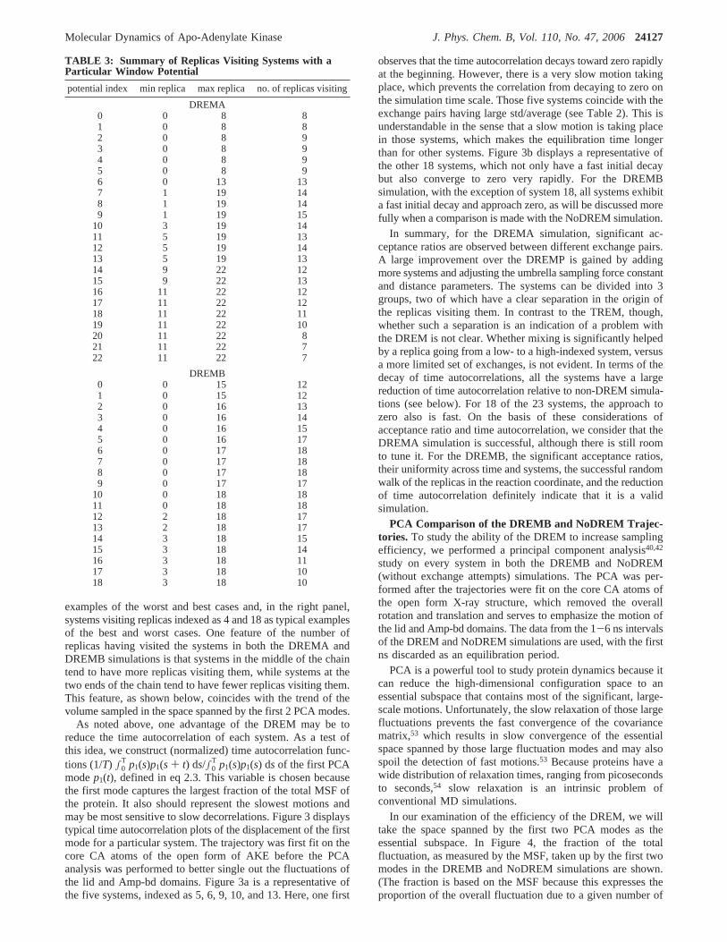
To examine the number of replicas visiting a particular system(with a particular window function), we list in Table 3 the rangeof replica indices for each system in the DREMA and DREMBsimulations. For the DREMA, no system has all the replicasvisiting it. There are basically three groups of systems: groupA (potential indices 0-6), where systems have low indexedreplicas visiting them, group B (potential indices 7-13), wheresystems have both high- and low-indexed replicas visiting them,and group C (potential indices 14-22), where systems havehigh-indexed replicas only visiting them. Group A consists ofsystems with equilibrium distances ranging from 5 to 7 Å, andonly replicas originating from systems with equilibrium dis-tances less than or equal to 11 Å visit group A. Most of thesystems in this group have about1/3 of the replicas visiting them,except the system with index 6 has1/2 of the replicas visitingit. Group C consists of systems with equilibrium distancesranging from 12 to 18 Å, and only replicas originating fromsystems with equilibrium distances larger than or equal to 9.5Å visit group C. While most of the systems in this group have1/2 the replicas visiting them, the last three systems have only1/3 of the replicas visiting them.

Figure 1 (left panel) displays three typical time trajectoriesof replica visits for systems with indices 3, 10, and 18. Figure1 (right panel) displays the complementary information of howselected replicas are visited by different systems for replicas 4,11, and 21. From the latter plot, one can conclude that, in aspecified range, the replica does undergo a random walk in thereaction coordinate for the DREMA simulation.

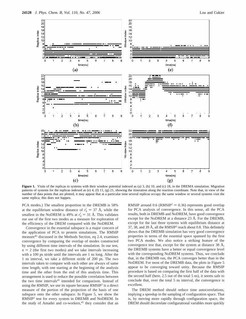
For the DREMB simulation, there are also no systems whereall the replicas visit a particular system, although all the systemshave more than half of the replicas visiting them. In contrastwith the DREMA simulation, all the systems have replicas withboth higher and lower indices visiting them, which results in arandom walk of replicas in the reaction coordinate along thewhole reaction coordinate chain. In Figure 2 (left panel), wepresent replica visits for systems indexed as 8 and 18 as typical

TABLE 2: Acceptance Ratio for the Time Span of theWhole Simulations

potential index acceptance ratioa acceptance ratiob std/average

DREMAc

0 T 1 0.444 0.445 0.1241 T 2 0.284 0.282 0.0612 T 3 0.269 0.270 0.1743 T 4 0.146 0.145 0.1824 T 5 0.293 0.292 0.0625 T 6 0.233 0.231 0.3456 T 7 0.130 0.130 0.4907 T 8 0.242 0.243 0.1858 T 9 0.327 0.328 0.1249 T 10 0.179 0.179 0.04410 T 11 0.239 0.237 0.18611 T 12 0.180 0.180 0.16712 T 13 0.160 0.160 0.35013 T 14 0.162 0.162 0.24414 T 15 0.197 0.196 0.17615 T 16 0.277 0.275 0.05316 T 17 0.249 0.250 0.06917 T 18 0.061 0.063 0.31418 T 19 0.121 0.120 0.22519 T 20 0.162 0.161 0.14820 T 21 0.240 0.240 0.11721 T 22 0.362 0.360 0.107

DREMBd

0 T 1 0.129 0.128 0.0771 T 2 0.117 0.115 0.0672 T 3 0.115 0.117 0.0633 T 4 0.165 0.157 0.0864 T 5 0.205 0.201 0.0745 T 6 0.192 0.192 0.0686 T 7 0.186 0.188 0.0857 T 8 0.208 0.206 0.1038 T 9 0.148 0.155 0.1269 T 10 0.123 0.119 0.06610 T 11 0.122 0.117 0.08411 T 12 0.106 0.115 0.08312 T 13 0.105 0.103 0.09013 T 14 0.128 0.126 0.05714 T 15 0.113 0.117 0.08715 T 16 0.114 0.115 0.16716 T 17 0.128 0.117 0.15417 T 18 0.117 0.121 0.094

a From the direct estimation method.b From the definite exchangemethod.c DREMA exchanges are attempted every 40 fs.d In the first7 ns of DREMB exchanges are attempted every 200 fs; for the last 2ns, every 40 fs.


examples of the worst and best cases and, in the right panel,systems visiting replicas indexed as 4 and 18 as typical examplesof the best and worst cases. One feature of the number ofreplicas having visited the systems in both the DREMA andDREMB simulations is that systems in the middle of the chaintend to have more replicas visiting them, while systems at thetwo ends of the chain tend to have fewer replicas visiting them.This feature, as shown below, coincides with the trend of thevolume sampled in the space spanned by the first 2 PCA modes.

As noted above, one advantage of the DREM may be toreduce the time autocorrelation of each system. As a test ofthis idea, we construct (normalized) time autocorrelation func-tions (1/T) ∫0

T p1(s)p1(s + t) ds/∫0T p1(s)p1(s) ds of the first PCA

modep1(t), defined in eq 2.3. This variable is chosen becausethe first mode captures the largest fraction of the total MSF ofthe protein. It also should represent the slowest motions andmay be most sensitive to slow decorrelations. Figure 3 displaystypical time autocorrelation plots of the displacement of the firstmode for a particular system. The trajectory was first fit on thecore CA atoms of the open form of AKE before the PCAanalysis was performed to better single out the fluctuations ofthe lid and Amp-bd domains. Figure 3a is a representative ofthe five systems, indexed as 5, 6, 9, 10, and 13. Here, one first

observes that the time autocorrelation decays toward zero rapidlyat the beginning. However, there is a very slow motion takingplace, which prevents the correlation from decaying to zero onthe simulation time scale. Those five systems coincide with theexchange pairs having large std/average (see Table 2). This isunderstandable in the sense that a slow motion is taking placein those systems, which makes the equilibration time longerthan for other systems. Figure 3b displays a representative ofthe other 18 systems, which not only have a fast initial decaybut also converge to zero very rapidly. For the DREMBsimulation, with the exception of system 18, all systems exhibita fast initial decay and approach zero, as will be discussed morefully when a comparison is made with the NoDREM simulation.

In summary, for the DREMA simulation, significant ac-ceptance ratios are observed between different exchange pairs.A large improvement over the DREMP is gained by addingmore systems and adjusting the umbrella sampling force constantand distance parameters. The systems can be divided into 3groups, two of which have a clear separation in the origin ofthe replicas visiting them. In contrast to the TREM, though,whether such a separation is an indication of a problem withthe DREM is not clear. Whether mixing is significantly helpedby a replica going from a low- to a high-indexed system, versusa more limited set of exchanges, is not evident. In terms of thedecay of time autocorrelations, all the systems have a largereduction of time autocorrelation relative to non-DREM simula-tions (see below). For 18 of the 23 systems, the approach tozero also is fast. On the basis of these considerations ofacceptance ratio and time autocorrelation, we consider that theDREMA simulation is successful, although there is still roomto tune it. For the DREMB, the significant acceptance ratios,their uniformity across time and systems, the successful randomwalk of the replicas in the reaction coordinate, and the reductionof time autocorrelation definitely indicate that it is a validsimulation.

PCA Comparison of the DREMB and NoDREM Trajec-tories. To study the ability of the DREM to increase samplingefficiency, we performed a principal component analysis40,42

study on every system in both the DREMB and NoDREM(without exchange attempts) simulations. The PCA was per-formed after the trajectories were fit on the core CA atoms ofthe open form X-ray structure, which removed the overallrotation and translation and serves to emphasize the motion ofthe lid and Amp-bd domains. The data from the 1-6 ns intervalsof the DREM and NoDREM simulations are used, with the firstns discarded as an equilibration period.

PCA is a powerful tool to study protein dynamics because itcan reduce the high-dimensional configuration space to anessential subspace that contains most of the significant, large-scale motions. Unfortunately, the slow relaxation of those largefluctuations prevents the fast convergence of the covariancematrix,53 which results in slow convergence of the essentialspace spanned by those large fluctuation modes and may alsospoil the detection of fast motions.53 Because proteins have awide distribution of relaxation times, ranging from picosecondsto seconds,54 slow relaxation is an intrinsic problem ofconventional MD simulations.

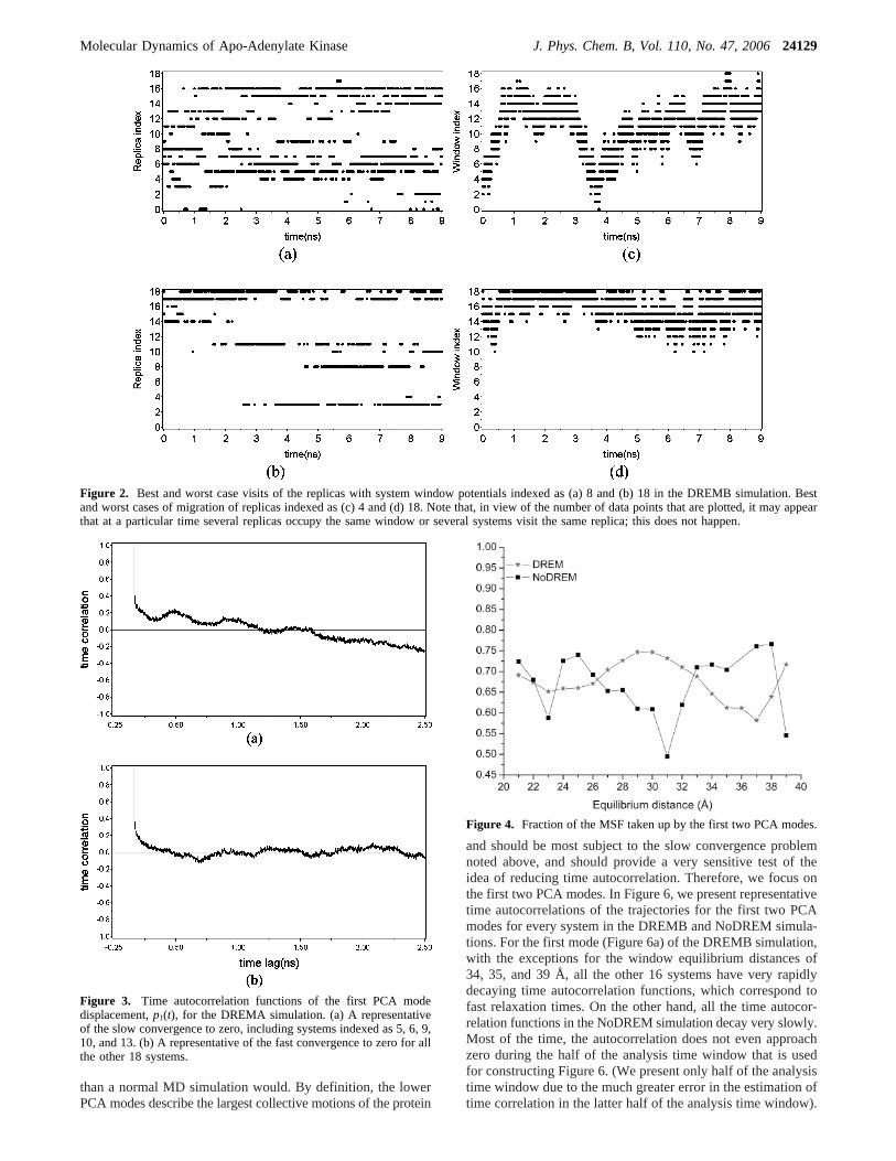
In our examination of the efficiency of the DREM, we willtake the space spanned by the first two PCA modes as theessential subspace. In Figure 4, the fraction of the totalfluctuation, as measured by the MSF, taken up by the first twomodes in the DREMB and NoDREM simulations are shown.(The fraction is based on the MSF because this expresses theproportion of the overall fluctuation due to a given number of

TABLE 3: Summary of Replicas Visiting Systems with aParticular Window Potential

potential index min replica max replica no. of replicas visiting

DREMA0 0 8 81 0 8 82 0 8 93 0 8 94 0 8 95 0 8 96 0 13 137 1 19 148 1 19 149 1 19 15

10 3 19 1411 5 19 1312 5 19 1413 5 19 1314 9 22 1215 9 22 1316 11 22 1217 11 22 1218 11 22 1119 11 22 1020 11 22 821 11 22 722 11 22 7

DREMB0 0 15 121 0 15 122 0 16 133 0 16 144 0 16 155 0 16 176 0 17 187 0 17 188 0 17 189 0 17 17

10 0 18 1811 0 18 1812 2 18 1713 2 18 1714 3 18 1515 3 18 1416 3 18 1117 3 18 1018 3 18 10


PCA modes.) The smallest proportion in the DREMB is 58%at the equilibrium window distance ofr0

i ) 37 Å, while thesmallest in the NoDREM is 49% atr0

i ) 31 Å. This validatesour use of the first two modes as a measure for exploration ofthe efficiency of the DREM compared with the NoDREM.

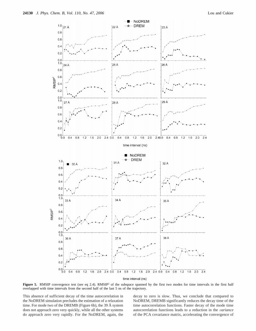
Convergence in the essential subspace is a major concern ofthe application of PCA to protein simulations. The RMSIPmeasure45 discussed in the Methods Section, eq 2.4, examinesconvergence by comparing the overlap of modes constructedby using different time intervals of the simulation. In our test,n ) 2 (the first two modes) and we take intervals increasingwith a 100 ps stride until the intervals are 1 ns long. After the1 ns interval, we take a different stride of 200 ps. The twointervals taken to compare with each other are always of sametime length, with one starting at the beginning of the analysistime and the other from the end of this analysis time. Thisarrangement is used to reduce the possible correlation betweenthe two time intervals45 intended for comparison. Instead ofusing the RMSIP, we use its square because RMSIP2 is a directmeasure of the portion of the projection of the basis of onesubspace onto the other subspace. In Figure 5, we show theRMSIP2 test for every system in DREMB and NoDREM. Inthe study of Amadei and co-workers,45 they consider that an

RMSIP around 0.6 (RMSIP2 ) 0.36) represents good overlapfor PCA analysis of convergence. In this sense, all the PCAresults, both in DREMB and NoDREM, have good convergenceexcept for the NoDREM at a distance 23 Å. For the DREMB,except for the last three systems with equilibrium distance at37, 38, and 39 Å, all the RMSIP2 reach about 0.8. This definitelyshows that the DREMB simulation has very good convergenceproperties in terms of the essential space spanned by the firsttwo PCA modes. We also notice a striking feature of theconvergence test that, except for the system at distance 38 Å,the DREMB systems have a better or equal convergence levelwith the corresponding NoDREM systems. Thus, we concludethat, in the DREMB run, the PCA converges better than in theNoDREM. For most of the DREMB data, the plots in Figure 5appear to be converging toward unity. Because the RMSIPprocedure is based on comparing the first half of the data withthe second half (here, 2.5 out of the total 5 ns), it seems safe toconclude that, over the total 5 ns interval, the convergence isexcellent.

The DREM method should reduce time autocorrelations,implying a speedup in the sampling of configuration space. Thatis, by moving more rapidly through configuration space, theDREM should decorrelate configurational variables more quickly

Figure 1. Visits of the replicas to systems with their window potential indexed as (a) 3, (b) 10, and (c) 18, in the DREMA simulation. Migrationpatterns of systems for the replicas indexed as (e) 4, (f) 11, (g) 21, showing the itineration along the reaction coordinate. Note that, in view of thenumber of data points that are plotted, it may appear that at a particular time several replicas occupy the same window or several systems visit thesame replica; this does not happen.


than a normal MD simulation would. By definition, the lowerPCA modes describe the largest collective motions of the protein

and should be most subject to the slow convergence problemnoted above, and should provide a very sensitive test of theidea of reducing time autocorrelation. Therefore, we focus onthe first two PCA modes. In Figure 6, we present representativetime autocorrelations of the trajectories for the first two PCAmodes for every system in the DREMB and NoDREM simula-tions. For the first mode (Figure 6a) of the DREMB simulation,with the exceptions for the window equilibrium distances of34, 35, and 39 Å, all the other 16 systems have very rapidlydecaying time autocorrelation functions, which correspond tofast relaxation times. On the other hand, all the time autocor-relation functions in the NoDREM simulation decay very slowly.Most of the time, the autocorrelation does not even approachzero during the half of the analysis time window that is usedfor constructing Figure 6. (We present only half of the analysistime window due to the much greater error in the estimation oftime correlation in the latter half of the analysis time window).

Figure 2. Best and worst case visits of the replicas with system window potentials indexed as (a) 8 and (b) 18 in the DREMB simulation. Bestand worst cases of migration of replicas indexed as (c) 4 and (d) 18. Note that, in view of the number of data points that are plotted, it may appearthat at a particular time several replicas occupy the same window or several systems visit the same replica; this does not happen.

Figure 3. Time autocorrelation functions of the first PCA modedisplacement,p1(t), for the DREMA simulation. (a) A representativeof the slow convergence to zero, including systems indexed as 5, 6, 9,10, and 13. (b) A representative of the fast convergence to zero for allthe other 18 systems.

Figure 4. Fraction of the MSF taken up by the first two PCA modes.


This absence of sufficient decay of the time autocorrelation inthe NoDREM simulation precludes the estimation of a relaxationtime. For mode two of the DREMB (Figure 6b), the 39 Å systemdoes not approach zero very quickly, while all the other systemsdo approach zero very rapidly. For the NoDREM, again, the

decay to zero is slow. Thus, we conclude that compared toNoDREM, DREMB significantly reduces the decay time of thetime autocorrelation functions. Faster decay of the mode timeautocorrelation functions leads to a reduction in theVarianceof the PCA covariance matrix, accelerating the convergence of

Figure 5. RMSIP convergence test (see eq 2.4). RMSIP2 of the subspace spanned by the first two modes for time intervals in the first halfoverlapped with time intervals from the second half of the last 5 ns of the trajectory.


the covariance matrix.53 The presence of slow decays in theNoDREM time autocorrelation functions for 34, 35, and 39 Åcould come from the slow relaxation of degrees of freedom otherthan the reaction coordinate, where other free energy barriersexist.

A complementary way to study the efficiency of the DREMis to compare the extent of the configuration space sampled byDREMB and NoDREM. Because the essential space of the PCAtakes up most of the protein motion, it is natural to examinethe volume of this essential space. This is the strategy used byZhang,55 as well as Sanbonmatsu and Garcia,56 in TREM

simulations. They found that their systems explored more space,based on the first two PCA modes, than the space explored bynormal MD, when comparable total simulation times are usedfor the comparison. We use the kernel density estimation methodwith a Gaussian kernel57 to estimate the probability density inthe plane spanned by the first two modes. Figure 7 presents thetypical probability density of the system in the plane spannedby the first two modes of the PCA analysis. We deliberatelymake the scale in the probability density axis the same, whilewe set the scales of the other axes according to their respectiveranges to contrast the differences between the DREMB and

Figure 6. (a) DREMB and NoDREM (no exchange attempts) time autocorrelations for PCA mode one, for 24, 34, 35, and 39 Å. The DREMB24 Å plot is representative of the fast decay DREMB systems. The DREMB systems with equilibrium window distances of 34, 35, and 39 Å showslower decay. The NoDREM systems for all equilibrium window distances exhibit slow decay behavior. (b) The DREMB and NoDREM timeautocorrelations for PCA mode two, for 24 and 39 Å, respectively. The 24 Å plot is representative of the fast decay DREMB systems. The 39 ÅDREMB system is the only one with slower decay. The NoDREM decays are slow for all equilibrium window distances.

Figure 7. Probability density in the plane spanned by the first two PCA modes for the 23 and 38 Å systems. The 23 Å result is representative ofall the systems other than the 38 Å system. (a) NoDREM. (b) DREMB. The 38 Å NoDREM and DREMB systems occupy almost the same area,while for all other systems, the DREMB probability is much more spread out than that for the NoDREM.


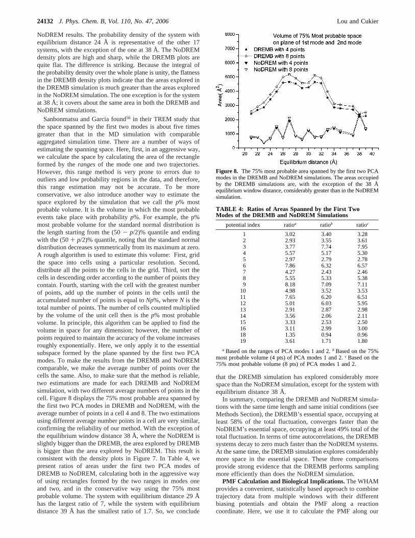
NoDREM results. The probability density of the system withequilibrium distance 24 Å is representative of the other 17systems, with the exception of the one at 38 Å. The NoDREMdensity plots are high and sharp, while the DREMB plots arequite flat. The difference is striking. Because the integral ofthe probability density over the whole plane is unity, the flatnessin the DREMB density plots indicate that the areas explored inthe DREMB simulation is much greater than the areas exploredin the NoDREM simulation. The one exception is for the systemat 38 Å; it covers about the same area in both the DREMB andNoDREM simulations.

Sanbonmatsu and Garcia found56 in their TREM study thatthe space spanned by the first two modes is about five timesgreater than that in the MD simulation with comparableaggregated simulation time. There are a number of ways ofestimating the spanning space. Here, first, in an aggressive way,we calculate the space by calculating the area of the rectangleformed by therangesof the mode one and two trajectories.However, this range method is very prone to errors due tooutliers and low probability regions in the data, and therefore,this range estimation may not be accurate. To be moreconservative, we also introduce another way to estimate thespace explored by the simulation that we call thep% mostprobable volume. It is the volume in which the most probableevents take place with probabilityp%. For example, the p%most probable volume for the standard normal distribution isthe length starting from the (50- p/2)% quantile and endingwith the (50+ p/2)% quantile, noting that the standard normaldistribution decreases symmetrically from its maximum at zero.A rough algorithm is used to estimate this volume: First, gridthe space into cells using a particular resolution. Second,distribute all the points to the cells in the grid. Third, sort thecells in descending order according to the number of points theycontain. Fourth, starting with the cell with the greatest numberof points, add up the number of points in the cells until theaccumulated number of points is equal toNp%, whereN is thetotal number of points. The number of cells counted multipliedby the volume of the unit cell then is thep% most probablevolume. In principle, this algorithm can be applied to find thevolume in space for any dimension; however, the number ofpoints required to maintain the accuracy of the volume increasesroughly exponentially. Here, we only apply it to the essentialsubspace formed by the plane spanned by the first two PCAmodes. To make the results from the DREMB and NoDREMcomparable, we make the average number of points over thecells the same. Also, to make sure that the method is reliable,two estimations are made for each DREMB and NoDREMsimulation, with two different average numbers of points in thecell. Figure 8 displays the 75% most probable area spanned bythe first two PCA modes in DREMB and NoDREM, with theaverage number of points in a cell 4 and 8. The two estimationsusing different average number points in a cell are very similar,confirming the reliability of our method. With the exception ofthe equilibrium window distance 38 Å, where the NoDREM isslightly bigger than the DREMB, the area explored by DREMBis bigger than the area explored by NoDREM. This result isconsistent with the density plots in Figure 7. In Table 4, wepresent ratios of areas under the first two PCA modes ofDREMB to NoDREM, calculating both in the aggressive wayof using rectangles formed by the two ranges in modes oneand two, and in the conservative way using the 75% mostprobable volume. The system with equilibrium distance 29 Åhas the largest ratio of 7, while the system with equilibriumdistance 39 Å has the smallest ratio of 1.7. So, we conclude

that the DREMB simulation has explored considerably morespace than the NoDREM simulation, except for the system withequilibrium distance 38 Å.

In summary, comparing the DREMB and NoDREM simula-tions with the same time length and same initial conditions (seeMethods Section), the DREMB’s essential space, occupying atleast 58% of the total fluctuation, converges faster than theNoDREM’s essential space, occupying at least 49% total of thetotal fluctuation. In terms of time autocorrelations, the DREMBsystems decay to zero much faster than the NoDREM systems.At the same time, the DREMB simulation explores considerablymore space in the essential space. These three comparisonsprovide strong evidence that the DREMB performs samplingmore efficiently than does the NoDREM simulation.

PMF Calculation and Biological Implications. The WHAMprovides a convenient, statistically based approach to combinetrajectory data from multiple windows with their differentbiasing potentials and obtain the PMF along a reactioncoordinate. Here, we use it to calculate the PMF along our

Figure 8. The 75% most probable area spanned by the first two PCAmodes in the DREMB and NoDREM simulations. The areas occupiedby the DREMB simulations are, with the exception of the 38 Åequilibrium window distance, considerably greater than in the NoDREMsimulation.

TABLE 4: Ratios of Areas Spanned by the First TwoModes of the DREMB and NoDREM Simulations

potential index ratioa ratiob ratioc

1 3.02 3.40 3.282 2.93 3.55 3.613 3.77 7.74 7.954 5.57 5.17 5.305 2.97 2.79 2.786 7.86 6.32 6.577 4.27 2.43 2.468 5.55 5.33 5.389 8.18 7.09 7.11

10 4.98 3.52 3.5311 7.65 6.20 6.5112 5.01 6.03 5.9513 2.91 2.87 2.9814 3.56 2.06 2.1115 3.33 2.53 2.5016 3.11 2.99 3.0018 1.35 0.94 0.9619 3.61 1.71 1.80

a Based on the ranges of PCA modes 1 and 2.b Based on the 75%most probable volume (4 pts) of PCA modes 1 and 2.c Based on the75% most probable volume (8 pts) of PCA modes 1 and 2.


selected reaction coordinate, the distance between the masscenters of residues 55 and 169, which are the residues that werelabeled in the energy transfer experiments7 and serve as amonitor of the Amp-bd domain-to-core distance. To make sureof the convergence of the PMF, we calculated the PMF for thetime corresponding to the first half and the second half of thetrajectory for the DREMA and DREMB data. In addition, twotrajectories (7 ns with the first ns discarded) of equilibriumdistance of 19 and 20 Å of the DREMP simulation are used toconnect the DREMA and DREMB simulations. Those twotrajectories are not in the problematic regions and have goodconverging distributions along the reaction coordinate for thedifferent time intervals.

The energy transfer experiments by Sinev et al.7 show thatAKE has an average reaction coordinate value of 31.0 Å forthe free form, 23.2 Å for the AMP-bound form, 18.7 Å for theMg2+-ATP bound form, and 11.5 Å for the AP5A (a mimic ofthe tertiary complex) bound form. The reaction coordinate valueis 28.7 Å in the free form X-ray structure and 11.5 Å in theAP5A-bound X-ray structure.1 Figure 9 displays the PMF. ThePMF from 10 to 39 Å converges very well, with somediscrepancy for reaction coordinate values less than 10 Å. Thelowest PMF value along the reaction coordinate occurs at 12.4Å. This distance is very close to the distance in the AP5A-boundform, and below, we show that this most stable state is similarto the closed form. Note that there is no barrier when one goesfrom 39 to 10 Å, and all the reaction coordinate distances thatcorrespond to the open, AMP-bound, and Mg2+-ATP-boundforms have at least a 2 kcal/mol difference with the minimumPMF value at 12.4 Å. This free energy difference translates toa ratio of occupation probabilities of about 28. However, notingthat the PMF from 18 to 30 Å is very flat compared to thePMF around 12 Å, it is more appropriate to make comparisonsbased on integrating the corresponding probability densities overreaction coordinate values. Thus, we integrate the probabilitydensity over the ranges 18 to 39 Å and 4 to 18 Å. The ratio ofthe second to the first integral is 3.88, which means that, if weconsider conformations with reaction coordinate range from 18to 39 Å as one state and 4 to 18 Å as another state, then thefree energy difference between these two states is only 0.81kcal/mol. The flatness of the PMF in the 18 to around 30 Årange is an indication of a large entropic contribution in thisregion. Distances larger than∼30 Å (the X-ray open formreaction coordinate distance is 28.7 Å) may correspond to

configurations that are becoming so “stretched” that theirprobabilities are decreasing due to decreasing entropic andincreasing energetic components of the free energy. The PMFresult is consistent with that found in the energy transferexperiment,7 where the free form does sample a very largenumber of conformations, as indicated by the large dispersionfound around the average reaction coordinate value.

The energy transfer experiment7 does not provide informationabout how the lid reacts to the changes in the reaction coordinatedistance. The reaction coordinate monitors the Amp-bd-to-coredistance. But, when AKE closes, there is also a large motionof the lid relative to the core, as is evident by comparing theopen and closed X-ray structures. In particular, the distancebetween the mass centers of the lid and core is 29.8 Å in thefree form and 20.3 Å in the AP5A-bound form X-ray structures.To explore this issue, we calculate PMF(x,r), the two-dimensional PMF in the plane spanned by the reaction coor-dinate,r, and the mass center distance between the lid and core,x. Figure 10 displays this two-dimensional PMF. The most stableconformation has a lid-to-core mass center distance of∼20.5Å and a reaction coordinate of∼12.0 Å, which are very closeto the AP5A-bound form distances. Note also that, from 18 to30 Å of the reaction coordinate, the PMF is not only flat alongthe reaction coordinate but also along the mass center lid-to-core distance. Most interestingly, in this region, the lid canfluctuate from the distance found for the free form (∼30 Å) tothe distance found for the AP5A-bound form (∼20 Å) in theX-ray data. This flatness in the lid-to-core region can compen-sate for the high PMF in the reaction coordinate directionrelative to the region around the minimum of 12 Å. If one startswith the largest value of the reaction coordinate and decreasesit, first, the lid can take on any conformation between the closedand open forms. Then, when the reaction coordinate reachesnear 18 Å, the fluctuations of the lid-to-core mass center distancebecome smaller. When the reaction coordinate decreases further,these fluctuations get even smaller. Finally, when the reactioncoordinate is around 12 Å, the lid is mostly in a closed form,with a relatively small proportion open. Along the lid-to-coredirection, there is a substantial free energy barrier separatingthese closed and open lid conformations.

The induced closure hypothesis that was proposed for AKEis based on the static X-ray structures of apo and various AKE1

complexes where, in the free form, AKE has an open lid andan open Amp-bd site. Then, when AMP binds, the lid and Amp-bd domains both close a little and, when AP5A binds, the lid

Figure 9. PMF for the first half, second half, and all of the trajectorydata.

Figure 10. PMF in the plane spanned by the lid-to-core mass centerdistance and the reaction coordinate.


and Amp-bd domains are completely closed. The above resultsshow that there is an alternative perspective, which does notcontradict the results of the X-ray based induced view. Insteadof a completely open conformation (both Amp-bd and lid open)in the free form, in our simulation, AKE can also exist in acompletely closed conformation (both Amp-bd and lid closed).Thus, even in the absence of ligands, AKE can sampleconformations similar to the completely closed form that isfound in the ternary (AP5A) complex. When the reactioncoordinate is in the range of the open form of the Amp-bddomain relative to the core, AKE also can sample multiple lidconformations, ranging between the closed- and open-lidconformers and, as the Amp-bd distance decreases, the lid-to-core distance decreases and its fluctuations are reduced.Furthermore, the existence of multiple conformations in the freeform is consistent with NMR experiments5 and also with thekinetic studies.2

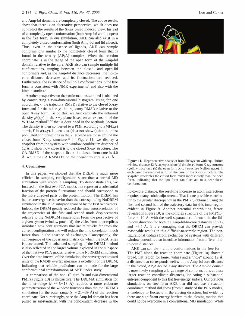
Another perspective on the conformations sampled is obtainedby constructing a two-dimensional histogram, using for onecoordinate,x, the trajectory RMSD relative to the closed X-rayform and for the other,y, the trajectory RMSD relative to theopen X-ray form. To do this, we first calculate the unbiaseddensityFu(x,y) in the x-y plane based on an extension of theWHAM method51,52 that is developed in the Methods Section.The density is then converted to a PMF according to PMF(x,y)) -kBT ln Fu(x,y). It turns out (data not shown) that the mostpopulated conformations in thex-y plane are those around theclosed-form X-ray structure.58 In Figure 11, we display asnapshot from the system with window equilibrium distance of12 Å to show how close it is to the closed X-ray structure. TheCA RMSD of the snapshot fit on the closed-form core is 4.0Å, while the CA RMSD fit on the open-form core is 7.0 Å.

4. Conclusions

In this paper, we showed that the DREM is much moreefficient in sampling configuration space than a normal MDsimulation with umbrella sampling. To demonstrate this, wefocused on the first two PCA modes that represent a substantialfraction of the protein fluctuations and should correspond tothe more directed parts of the protein motion. The DREM hasbetter convergence behavior than the corresponding NoDREMsimulation in the PCA subspace spanned by the first two vectors.Indeed, the DREM greatly reduced the time autocorrelation ofthe trajectories of the first and second mode displacementsrelative to the NoDREM simulations. From the perspective ofa given system (window potential), the visits from other replicasintroduce new configurations that are relatively far from thecurrent configuration and will reduce the time correlation muchfaster than in the absence of exchanges. Consequently, theconvergence of the covariance matrix on which the PCA reliesis accelerated. The enhanced sampling of the DREM methodis also reflected in the larger volume explored in the subspaceof the first two PCA modes relative to the NoDREM simulation.Over the time interval of the simulation, the convergence towardunity of the RMSIP overlap measure is excellent for the DREM,indicating that reliable predictions can be made for the largeconformational transformation of AKE under study.

A comparison of the one- (Figure 9) and two-dimensionalPMFs (Figure 10) is instructive. The DREMA simulation forthe inner range (r ∼ 5-18 Å) required a more elaborateparametrization of the window functions than did the DREMBsimulation for the outer range (r ∼ 21-39 Å) of the reactioncoordinate. Not surprisingly, once the Amp-bd domain has beenpulled in substantially, with the concomitant decrease in the

lid-to-core distance, the resulting increase in atom interactionsrequires many subtle adjustments. That is one possible contribu-tor to the greater discrepancy in the PMF(r) obtained using thefirst and second half of the trajectory data for this inner regionevident in Figure 9. Another potential contributing factor,revealed in Figure 10, is the complex structure of the PMF(x,r)for r < 10 Å, with the well-separated conformers in the lid-to-core direction for both the Amp-bd-to-core distances of∼12and ∼8.5 Å. It is encouraging that the DREM can providereasonable results in this difficult-to-sample region. The con-figurational updates from exchanges of systems with differentwindow potentials also introduce information from different lid-to-core distances.

AKE can sample multiple conformations in the free form.The PMF along the reaction coordinate (Figure 10) shows abroad, flat region for larger values and a “hole” around 12 Å,a distance that corresponds well with the Amp-bd core distancein the closed, AP5A-bound X-ray structure. The Amp-bd domainis most likely sampling a large range of conformations at theselarger reaction coordinate distances, indicating a substantialentropic component to this flat free energy surface. Our previoussimulations on free form AKE that did not use a reactioncoordinate method did show (from a study of the PCA modes)a tendency to fluctuate in the closing direction, but evidentlythere are significant energy barriers to the closing motion thatcould not be overcome in a conventional MD simulation. While

Figure 11. Representative snapshot from the system with equilibriumwindow distance 12 Å superposed on (a) the closed-form X-ray structure(yellow trace) and (b) the open form X-ray structure (yellow trace). Ineach case, the snapshot is fit on the core of the X-ray structure. Thesnapshot resembles the closed form much more closely than the openform, indicating that the apo form can fluctuate to a near-closedconformation.


the small free energy difference (∼0.8 kcal/mol) favoring“closed” (4-18 Å) versus “open” (18-39 Å) that we find isconsistent with the experimental data, it must be stressed that,allowing for the quality of MD force fields and the differencesbetween experimental and simulation systems, it is only safeto conclude that there is some reasonable fraction of “closed”states.

Examination of conformations along the reaction coordinatetrajectory showed that, in addition to ones similar to the AP5A-bound conformation, there are conformations in which the lid-core distance ranges from the corresponding distance in the freeform X-ray structure to the one in the AP5A-bound X-raystructure. The two-dimensional PMF in the reaction coordinateand lid-core distance variables (Figure 10) shows that, as thereaction coordinate distance decreases, AKE’s lid progressivelychanges its motion from readily fluctuating between its openand closed conformations toward more constrained fluctuationsuntil it mainly stays in the closed-form conformation when thereaction coordinate is around 12 Å. It is interesting that, in thesimulation protocol where the Amp-bd-to-core distance isreduced gradually, the lid-to-core distance responds to thisreduction by also decreasing, and does so in a manner thateventually produces conformations similar to the closed-formX-ray structure. Furthermore, as these distances decrease, therange of lid-to-core distances sampled decreases, in agreementwith the reduction in fluctuations as successive ligands are boundin the energy transfer experiments. The correlation between thesedistances does not contradict the random bi bi mechanismsuggested for AKs.59 That is, once ligand free closed conforma-tions are sampled, the ligands can then bind in random order,and both are required for the final catalytically competentstructure.

The open-to-closed transition in AKE has been studied bymethods that are generalizations of the elastic network model(ENM) whereby the path between open and closed forms isobtained by mixing these two endpoints.21,20 Both studiesconclude that the lid and Amp-bd domains can rearrange withouta great (free) energy penalty, while the core is quite stable duringthis transition. Maragakis and Karplus,21 starting from the openform, find that first mainly the lid closes and then the Amp-bddomain closes. They attribute the order to the small energy costof moving the lid, with its flexible hinge connections to thecore domain. They identify hinges for the open-to-closedpathway that are similar to those found using the open andclosed X-ray structures. Because our simulation uses a reactioncoordinate, the Amp-bd core distance, we cannot obtain an orderof closing. Note that our result does not rely on using a specifiedclosed form endpoint; the closed form we obtain emerges justfrom the distance restraint on the Amp-bd-to-core distance. Wedetermined the hinges between the open-form X-ray structureand the closed structure snapshot displayed in Figure 11, usingthe DynDom program.60 The results show that there are hinge-bending regions around the beginning (residues 117-123) andend (residues 153-167) of the lid domain and around thebeginning (residues 26-29) and end (residues 64-66) of theAmp-bd domain. These are quite close to those found in theENM work21 that used DynDom and similar to those found byother methods using open (beef heart) and closed (AKE) X-raystructures.10

The ease with which AK can sample a large conformationalspace is supported by the MD and ENM approaches. In thisregard, a recent investigation of chimeric forms of adenylatekinase that are constructed by switching regions of mesophilicand thermophilic varieties showed that the core is mainly

involved in thermal stability while the lid and Amp-bd domainsare not.61 In the DREM simulations, the core structure is wellmaintained at all stages along the reaction coordinate, indicatingthe stability of the core during the large-scale rearrangementsof lid and Amp-bd domains, which is consistent with the chimeraresults. Furthermore, in a previous MD simulation of apo AKE,18

we found that raising the simulation temperature induced anincrease in the mobility of the lid and Amp-bd domains whilethe core stayed stable.

The scenario presented above provides an attractive alternativeto the induced fit hypothesis, where ligand binding is requiredfor closing AKE. Instead, what we find is that the apo form ofAKE can sample a broad range of conformational states, someof which resemble the final closed form. These conformationsmay be more advantageous for ligand binding by requiringsmaller protein rearrangements (with a reduced energeticrequirement) than would be necessary in the more open forms.Of course, in the process of binding ligands, an entropic penaltyfrom restricting the space available to the ligands must becompensated for by the formation of ligand-protein interactions.These final rearrangements must occur even if the protein is ina state resembling the ligand-bound closed form.

Acknowledgment. This work is supported by the NIH (grantno. GM62790). The simulations were carried out on theMichigan Center for Biological Information Linux cluster atMichigan State University.

Appendix A

The average acceptance ratio is defined as

with the transition probability satisfying the detailed balancecondition of eq 2.1. For a Metropolis Monte Carlo transitionprobability,

with, for a general HREM simulation,

eq A.1 can be resolved as

The second integral’s area restriction can be expressed interms of the definitely accepted region with the use of thedetailed balance condition since

pacc) ∫ dR0 ∫ dR1 P0(R0)P1(R1)R(R0R1 f R1R0) (A.1)

R(R0R1 f R1R0) ) 1 (∆ e 0)

) exp(-∆) (∆ > 0)(A.2a)

∆(X iX j f X jX i) ) â[(Ei(X j) + Ej(X i)) - (Ei(X i) + Ej(X j))]

(A.2b)

pacc) ∫∫R(R0R1fR1R0))1

dR0 dR1P0(R0)P1(R1) +

∫∫R(R0R1fR1R0)<1

dR0 dR1P0(R0)P1(R1)R(R0R1 f R1R0)

(A.3)

∫∫R(R0R1fR1R0)<1

dR0 dR1P0(R0)P1(R1)R(R0R1 f R1R0)

) ∫∫R(R0R1fR1R0)<1

dR0 dR1P0(R1)P1(R0) (A.4)


Here, we have used the property that the “reverse” transitionprobability must be unity for this region of integration. Then,interchange of integration variablesR0 f X1, R1 f X0 in eqA.4 provides

Adding this to the first integration region result in eq A.3 yieldseq 2.7.

A generalization of eq 2.7 can be devised that may be of usefor certain types of replica exchange rules. The above equationwill not hold if there exists afinite area where∆ ) 0 in theCartesian product spaceX0 × X1. When ∆ ) 0, R(X0X1 fX1X0) ) R(X1X0 f X0X1) ) 1. For example, in a temperatureexchange method, where two systems have the same temper-ature, the system must exchange with probability 1 on everyattempt. So, according to eq A.5, the acceptance ratio frommethod 2 will double the acceptance ratio of method 1. Thisproblem comes from the fact that, under the whole area formedby Cartesian productX0 × X1, ∆ ≡ 0. Then the area where∆) 0 will double count the probability. The error comes fromthe reasoning in eq A.5 that the area whereR(X1X0 f X0X1)< 1 is equivalent to the area whereR(X0X1 f X1X0) ) 1.Apparently, if there exists a finite area whereR(X0X1 f X1X0)) R(X1X0 f X0X1) ) 1, then the area will be double counted.A more general form forpacc based on this reasoning is

In the case of the DREM and the TREM, the second part ofthis equation is zero because there is no area where∆(X0X1 fX1X0) ) 0, because∆(X0X1 f X1X0) ) 0 means a line (onelower dimension in the Cartesian product spaceX0 × X1) andthe probability density function is assumed to be continuous.This issue was also identified in a recent work, and a similarremedy was proposed.50

A circumstance where eq A.6 would be necessary would bein a HREM, where the exchange rule parameter∆(X0X1 fX1X0) would depend on a cutoff energy. That is, an energythreshold would first be evaluated in order to decide if theHamiltonians for systems 0 and 1 are different. That would leadto a finite area of configuration space where∆(X0X1 f X1X0)) 0 and necessitates the use of eq A.6.

Appendix B

We want to show that the expected value of the estimatedprobability that the coordinate values (s,t) lie in the rectangle(x,y) × (x + ∆x,y + ∆y) is unbiased. That is, the average ofthe estimated probability is the true value when it is constructedaccording to the window method we used in the Results Section.The estimated probabilityP(u) is expressed as

where the indicator function is

and

Here, for windoww, Ww(r) is the window function,nw is thenumber of points in the window, andfw is the correspondingfree energy. Now, the expected value of the estimated probabilityis

whereFw(b)(s,t,r) is the biased distribution for windoww.

According to Souaille and Roux,52 the WHAM methodprovides the connection

between theFw(b)(s,t,r) andF(u)(s,t,r), the unbiased distribution.

Therefore, using eq B.5 in B.4,

So, the estimated probability is unbiased.

References and Notes

(1) Schulz, G. E.; Muller, C. W.; Diederichs, K.J. Mol. Biol. 1990,213, 627.

(2) Sheng, X. R.; Li, X.; Pan, X. M.J. Biol. Chem.1999, 274, 22238.

∫∫R(R0R1fR1R0)<1

dR0 dR1P0(R1)P1(R0)

) ∫∫R(X1X0fX0X1)<1

dX0 dX1P0(X0)P1(X1)

) ∫∫R(X0X1fX1X0))1

dX0 dX1P0(X0)P1(X1) (A.5)

pacc) 2∫∆(X0X1fX1X0)e0dX1 dX0P0(X0)P1(X1) -

∫∆(X0X1fX1X0))0dX1 dX0P0(X0)P1(X1) (A.6)

P(u)((s,t) ∈ (x,y) × (x + ∆x,y + ∆y)) )

∑w)1

N

∑j)1

nw I((xjw,yj

w) ∈ (x,y) × (x + ∆x,y + ∆y))

G(rjw)

(B.1)

I((s,t) ∈ (x,y) × (x + ∆x,y + ∆y)) )

0 (s,t) ∉ (x,y) × (x + ∆x,y + ∆y)1 (s,t) ∈ (x,y) × (x + ∆x,y + ∆y)

(B.2)

G(r) ) ∑w)1

N

nw e-â(Ww(r) - fw) (B.3)

E[P(u)((s,t) ∈ (x,y) × (x + ∆x,y + ∆y))] )

∑w)1

N

E[∑j)1

nw I((xjw,yj

w) ∈ (x,y) × (x + ∆x,y + ∆y))

G(rjw) ]

) ∑w)1

N

nwEw[I((s,t) ∈ (x,y) × (x + ∆x,y + ∆y))

G(r) ]) ∑

w)1

N

nw ∫∫∫ I((s,t) ∈ (x,y)×(x+∆x,y+∆y))

G(r)Fw

(b)(s,t,r) ds

dt dr

) ∫∫∫ ∑w)1

N nwFw(b)(s,t,r)

G(r)I((s,t) ∈ (x,y) × (x + ∆x,y + ∆y))

(B.4)

∑w)1

N nwFw(b)(s,t,r)

G(r)) F(u)(s,t,r) (B.5)

E[P(u)((s,t) ∈ (x,y) × (x + ∆x,y + ∆y))]

) ∫∫∫ F(u)(s,t,r)I((s,t) ∈ (x,y)× (x+ ∆x,y + ∆y)) ds dt dr

) ∫(s,t)∈(x,y)×(x+∆x,y+∆y),r

∫∫ F(u)(s,t,r) ds dt dr

) P(u)((s,t) ∈ (x,y) × (x + ∆x,y + ∆y)) (B.6)


(3) Han, Y.; Li, X.; Pan, X. M.FEBS Lett.2002, 528, 161.(4) Zhang, H. J.; Sheng, X. R.; Niu, W. D.; Pan, X. M.; Zhou, J. M.

J. Biol. Chem.1998, 273, 7448.(5) Burlacu-Miron, S.; Gilles, A. M.; Popescu, A.; Baˆrzu, O.; Craescu,

C. T. Eur. J. Biochem.1999, 264, 765.(6) Wolf-Watz, M.; Thai, V.; Henzler-Wildman, K.; Hadjipavlou, G.;

Eisenmesser, E. Z.; Kern, D.Nat. Struct. Mol. Biol.2004, 11, 945.(7) Sinev, M. A.; Sineva, E. V.; Ittah, V.; Haas, E.Biochemistry1996,

35, 6425.(8) Byeon, L.; Shi, Z.; Tsai, M. D.Biochemistry1995, 34, 3172.(9) Koshland, D. E.Proc. Natl. Acad. Sci. U.S.A.1958, 44, 98.

(10) Gerstein, M.; Schulz, G.; Chothia, C.J. Mol. Biol.1993, 229, 494.(11) Kumar, S.; Sham, Y. Y.; Tsai, C.-J.; Nussinov, R.Biophys. J.2001,

80, 2439.(12) Hayward, S.J. Mol. Biol. 2004, 339, 1001.(13) Eisenmesser, E. Z.; Millet, O.; Labeikovsky, W.; Korzhnev, D. M.;

Wolf-Watz, M.; Bosco, D. A.; Skalicky, J. J.; Kay, L. E.; Kern, D.Nature2005, 438, 117.

(14) Taniuchi, H.; Anfinsen, C. B.J. Biol. Chem.1966, 241, 4366.(15) Markley, J. L.; Williams, M. N.; Jardetzky, O.Proc. Natl. Acad.

Sci. U.S.A.1970, 65, 645.(16) Chazin, W. J.; Kordel, J.; Drakenberg, T.; Thulin, E.; Brodin, P.;

Grundstrom, T.; Forsen, S.Proc. Natl. Acad. Sci. U.S.A.1989, 86, 2195.(17) Wilson, M. A.; Brunger, A. T.J. Mol. Biol. 2000, 301, 1237.(18) Lou, H. F.; Cukier, R. I.J. Phys. Chem. B2006, 110, 12796.(19) Temiz, N. A.; Meirovitch, E.; Bahar, I.Proteins: Struct., Funct.,

Bioinf. 2004, 57, 468.(20) Miyashita, O.; Onuchic, J. N.; Wolynes, P. G.Proc. Natl. Acad.

Sci. U.S.A.2003, 100, 12570.(21) Maragakis, P.; Karplus, M.J. Mol. Biol. 2005, 352, 807.(22) Berg, B. A.; Neuhaus, T.Phys. Lett. B1991, 267, 249.(23) Hansmann, U. H. E.; Okamoto, Y.; Eisenmenger, F.Chem. Phys.

Lett. 1996, 259, 321.(24) Lyubartsev, A. P.; Martsinovski, A. A.; Shevkunov, S. V.;

Vorontsov-Velyaminov, P. N.J. Chem. Phys.1992, 96, 1776.(25) Lyubartsev, A.; Laaksonen, A.Appl. Parallel Comput.1998, 1541,

296.(26) Swendsen, R. H.; Wang, J. S.Phys. ReV. Lett. 1986, 57, 2607.(27) Sugita, Y.; Okamoto, Y.Chem. Phys. Lett.1999, 314, 141.(28) Hansmann, U. H. E.Chem. Phys. Lett.1997, 281, 140.(29) Geyer, C. J. Markov Chain Monte Carlo Maximum Likelihood. In

Computing Science and Statistics: Proceedings of the 23rd Symposium onthe Interface; Keramidas, E. M., Ed.; Interface Foundation: Fairfax Station, VA, 1991.

(30) Wang, J. S.; Swendsen, R. H.Prog. Theor. Phys. Suppl.2005, 317.(31) Hukushima, K.; Nemoto, K.J. Phys. Soc. Jpn.1996, 65, 1604.(32) Fukunishi, H.; Watanabe, O.; Takada, S.J. Chem. Phys.2002, 116,

9058.(33) Frenkel, D.; Smit, B.Understanding Molecular Simulation: From

Algorithms to Applications; Academic: San Diego, 1996.

(34) Predescu, C.; Predescu, M.; Ciobanu, C. V.J. Phys. Chem. B2005,109, 4189.

(35) Sugita, Y.; Kitao, A.; Okamoto, Y.J. Chem. Phys.2000, 113, 6042.(36) van Gunsteren, W. F.; Billeter, S. R.; Eising, A. A.; Hu¨nenberger,

P. H.; Kruger, P.; Mark, A. E.; Scott, W. R. P.Biomolecular Simulation:The GROMOS96 Manual and User Guide; Vdf Hochschulverlag AG ander ETH: Zurich, 1996.

(37) Essmann, U.; Perera, L.; Berkowitz, M. L.; Darden, T.; Lee, H.;Pedersen, G. L.J. Chem. Phys.1995, 103, 8577.

(38) Muller, C. W.; Schlauderer, G. J.; Reinstein, J.; Schulz, G. E.Structure1996, 4, 147.

(39) Cox, T. F.; Cox, M. A. A.Multidimensional Scaling, 2nd ed.;Chapman & Hall: Boca Raton, FL, 2001.

(40) Garcı´a, A. E.Phys. ReV. Lett. 1992, 68, 2696.(41) Garcı´a, A. E.; Blumenfeld, R.; Hummer, G.; Krumhansl, J. A.

Physica D1997, 107, 225.(42) Amadei, A.; Linssen, A. B. M.; Berendsen, H. J. C.Proteins:

Struct., Funct., Genet.1993, 17, 412.(43) Romo, T. D.; Clarage, J. B.; Sorensen, D. C.; Phillips, G. N.

Proteins: Struct., Funct., Genet.1995, 22, 311.(44) Teodoro, M. L.; Phillips, G. N.; Kavraki, L. E.J. Comput. Biol.

2003, 10, 617.(45) Amadei, A.; Ceruso, M. A.; Di Nola, A.Proteins: Struct., Funct.,

Genet.1999, 36, 419.(46) Hess, B.Phys. ReV. E 2000, 62, 8438.(47) Hess, B.Phys. ReV. E 2002, 65, 031910.(48) Lou, H.Analyzer, version 1.0; East Lansing, MI, 2005.(49) Kofke, D. A.J. Chem. Phys.2002, 117, 6911.(50) Chempath, S.; Predescu, C.; Bell, A. T.J. Chem. Phys.2006, 124,

234101.(51) Kumar, S.; Bouzida, D.; Swendsen, R. H.; Kollman, P. A.;

Rosenberg, J. M.J. Comput. Chem.1992, 13, 1011.(52) Souaille, M.; Roux, B.Comput. Phys. Commun.2001, 135, 40.(53) Balsera, M. A.; Wriggers, W.; Oono, Y.; Schulten, K.J. Phys.

Chem.1996, 100, 2567.(54) McCammon, A.; Harvey, S. C.Dynamics of Proteins and Nucleic

Acids; Cambridge University Press: Cambridge, 1987.(55) Zhang, W.; Wu, C.; Duan, Y.J. Chem. Phys.2005, 123.(56) Sanbonmatsu, K. Y.; Garcia, A. E.Proteins: Struct., Funct., Genet.

2002, 46, 225.(57) Silverman, B. W.Density Estimation for Statistics and Data

Analysis; Chapman and Hall: London, New York, 1986.(58) Muller, C. W.; Schulz, G. E.J. Mol. Biol. 1992, 224, 159.(59) Walsh, C.Enzymatic Reaction Mechanisms; W. H. Freeman: San

Francisco, 1979.(60) Hayward, S.; Lee, R. A.J. Mol. Graphics Modell.2002, 21, 181.(61) Bae, E.; Phillips, G. N.Proc. Natl. Acad. Sci. U.S.A.2006, 103,

2132.


molecular dynamics of apo-adenylate kinase: a … 110...molecular dynamics of apo-adenylate kinase:...

Documents