module 1.4: point loading of a 2d cantilever beam

UCONN ANSYS –Module 1.4

Module 1.4: Point Loading of a 2D Cantilever Beam

Table of Contents Page Number

Problem Description 2

Theory 2

Geometry 3

Preprocessor 7

Element Type

Real Constants and Material Properties 9

Meshing 10

Loads 11

Solution 14

General Postprocessor 15

Results 19

Validation 21


Problem Description

Nomenclature:

L =110m Length of beam

b =10m Cross Section Base

h =1 m Cross Section Height

P=1000N Point Load

E=70GPa Young’s Modulus of Aluminum at Room Temperature

=0.33 Poisson’s Ratio of Aluminum

In this module, we will be modeling an Aluminum cantilever beam with a point load at the

end with two dimensional elements in ANSYS Mechanical APDL. Since the exact solution to

this problem is numerical, we will be using beam theory and mesh independence as our

key validation requirements. The beam theory for this analysis is shown below:

Theory

Von Mises Stress

Assuming plane stress, the Von Mises Equivalent Stress can be expressed as:

(1.4.1)

During our analysis, we will be analyzing the set of nodes through the top center of the cross

section of the beam:

Due to symmetric loading about the yz cross sections, analyzing the nodes through the top center

will give us deflections that approximate beam theory. Additionally, since the nodes of choice

are located at the top surface of the beam, the shear stress at this location is zero.

( . (1.4.2)

Using these simplifications, the Von Mises Equivelent Stress from equation 1 reduces to:

(1.4.3)

y

x

. . . . . (.) . . . . .

y

z


Bending Stress is given by:

(1.4.4)

Where

and

. From statics, we can derive:

(1.4.5)

(1.4.6)

With Maximum Stress at:

= 66 KPa (1.4.7)

Beam Deflection

As in module 1.1, the beam equation to be solved is:

(1.4.8)

Using Shigley’s Mechanical Engineering Design, the beam deflection is:

(1.4.9)

With Maximum Deflection at:

= 7.61mm (1.4.10)

Geometry

Opening ANSYS Mechanical APDL

1. On your Windows 7 Desktop click the Start button

2. Under Search Programs and Files type “ANSYS”

3. Click on Mechanical APDL (ANSYS) to start

ANSYS. This step may take time.

1

2

3


Preferences

1. Go to Main Menu -> Preferences

2. Check the box that says Structural

3. Click OK

1

2

3


Keypoints

Since we will be using 2D Elements, our goal is to model the length and width of the beam. The

thickness will be taken care of later as a real constant property of the shell element we will be

using.

1. Go to Main Menu -> Preprocessor -> Modeling -> Create ->

Keypoints -> On Working Plane

2. Click Global Cartesian

3. In the box underneath, write: 0,0,0 This will create a keypoint at the

Origin.

4. Click Apply

5. Repeat Steps 3 and 4 for the following points in order: 0,0,10

110,0,10

110,0,0

6. Click Ok

Let’s check our work.

7. Click the Dynamic Model Mode icon. On the graphics window,

right click and drag the cursor down. You should now be able to see

all four keypoints you have just created:

8. The Triad in the top left corner is blocking keypoint 1. To get rid of the triad, type

/triad,off in Utility Menu -> Command Prompt

9. Go to Utility Menu -> Plot -> Replot

2

3

4

6

7

8


Your graphics window should look as shown:

SAVE_DB

Since we have made considerable progress thus far, we will create a temporary save file for our

model. This temporary save will allow us to return to this stage of the tutorial if an error is made.

1. Go to Utility Menu -> ANSYS Toolbar ->SAVE_DB This creates a save checkpoint

2. If you ever wish to return to this checkpoint in your model generation, go to Utility

Menu -> RESUM_DB

Areas

1. Go to Main Menu -> Preprocessor -> Modeling -> Create ->

Areas -> Arbitrary -> Through KPs

2. Select Pick

3. Select Min, Max, Inc

4. In the space below, type 1,4,1. If you are familiar with programming,

the ‘Min,Max, Inc’ acts as a FOR loop, connecting nodes 1 through 4

incrementing (Inc) by 1.

5. Click OK

WARNING: If you declared your keypoints in anther order than specified

in this tutorial, you may not be able to loop. In which case, plot the

keypoints and pick them under List of Items in a “connect the dots” order

that would create a rectangle.

WARNING: It is VERY HARD to delete or modify inputs and commands to your model

once they have been entered. Thus it is recommended you use the SAVE_DB and

RESUM_DB functions frequently to create checkpoints in your work. If salvaging your

project is hopeless, going to Utility Menu -> File -> Clear & Start New -> Do not read file

->OK is recommended. This will start your model from scratch.

2

3

4

5


6. Go to Plot -> Areas

7. Click the Top View tool

8. Go to Utility Menu -> Ansys Toolbar -> SAVE_DB

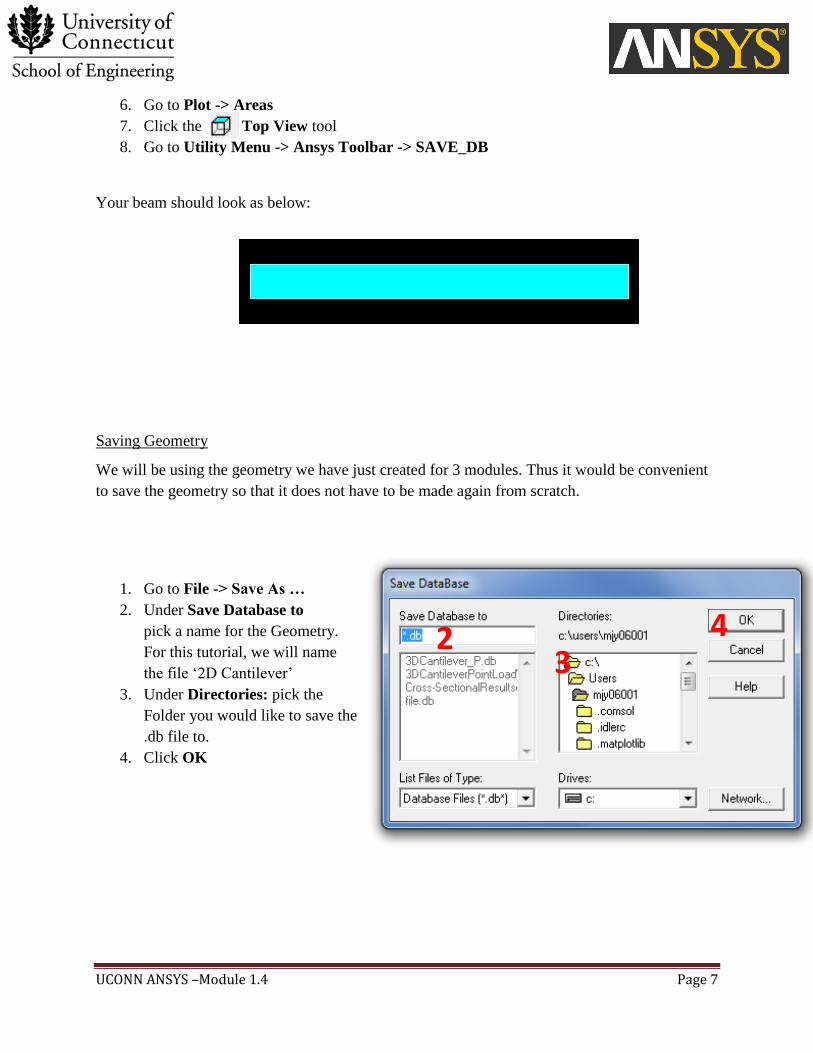
Your beam should look as below:

Saving Geometry

We will be using the geometry we have just created for 3 modules. Thus it would be convenient

to save the geometry so that it does not have to be made again from scratch.

1. Go to File -> Save As …

2. Under Save Database to

pick a name for the Geometry.

For this tutorial, we will name

the file ‘2D Cantilever’

3. Under Directories: pick the

Folder you would like to save the

.db file to.

4. Click OK

2

3

4


Preprocessor

Element Type

1. Go to Main Menu -> Preprocessor ->

Element Type -> Add/Edit/Delete

2. Click Add

3. Click Shell -> 4node 181 the elements

that we will be using are four node

elements with six degrees of freedom.

4. Click OK

5. For more information on SHELL 181,

click the Help button to open ANSYS

Help

6. Go to ANSYS 12.1 Help -> Search ->

Keyword Search -> type

‘SHELL181’ and press Enter

7. Go to Search Options ->SHELL181

the element description should

appear in the right portion of the

screen. out when done.

8. Click Close

9. Go to Utility Menu -> ANSYS

Toolbar -> SAVE_DB

\

2

3

4

5

6

7

8

7


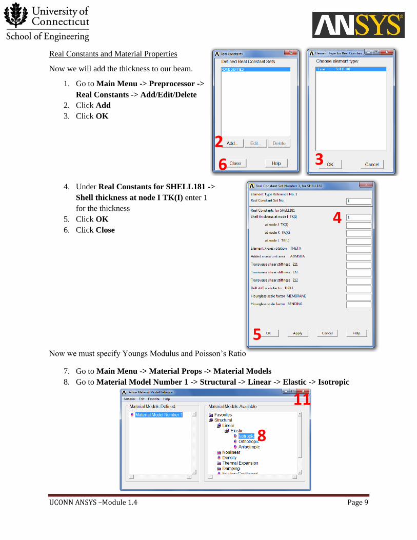
Real Constants and Material Properties

Now we will add the thickness to our beam.


Real Constants -> Add/Edit/Delete

2. Click Add

3. Click OK

4. Under Real Constants for SHELL181 ->

Shell thickness at node I TK(I) enter 1

for the thickness

5. Click OK

6. Click Close

Now we must specify Youngs Modulus and Poisson’s Ratio

7. Go to Main Menu -> Material Props -> Material Models

8. Go to Material Model Number 1 -> Structural -> Linear -> Elastic -> Isotropic

2

3

4

5

6

8

11


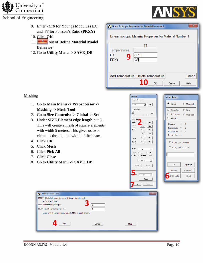
9. Enter 7E10 for Youngs Modulus (EX)

and .33 for Poisson’s Ratio (PRXY)

10. Click OK

11. out of Define Material Model

Behavior

12. Go to Utility Menu -> SAVE_DB

Meshing


Meshing -> Mesh Tool

2. Go to Size Controls: -> Global -> Set

3. Under SIZE Element edge length put 5.

This will create a mesh of square elements

with width 5 meters. This gives us two

elements through the width of the beam.

4. Click OK

5. Click Mesh

6. Click Pick All

7. Click Close


9

10

2

3

4

5

6

7


Your mesh should look like this:

Loads

Displacements

1. Go to Utility Menu -> Plot -> Nodes

2. Go to Utility Menu -> Plot Controls -> Numbering…

3. Check NODE Node Numbers to ON

4. Click OK

The graphics area should look as below:

This is one of the main advantages of ANSYS Mechanical APDL vs ANSYS Workbench in that we

can visually extract the node numbering scheme. As shown, ANSYS numbers nodes at the left

corner, the right corner, followed by filling in the remaining nodes from left to right.

3

4


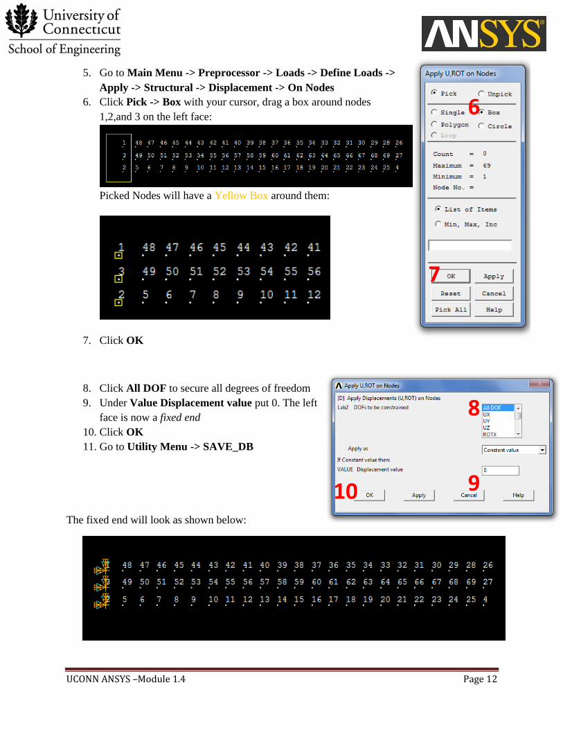
5. Go to Main Menu -> Preprocessor -> Loads -> Define Loads ->

Apply -> Structural -> Displacement -> On Nodes

6. Click Pick -> Box with your cursor, drag a box around nodes

1,2,and 3 on the left face:

Picked Nodes will have a Yellow Box around them:

7. Click OK

8. Click All DOF to secure all degrees of freedom

9. Under Value Displacement value put 0. The left

face is now a fixed end

10. Click OK


The fixed end will look as shown below:

6

7

8

9

10


Point Load

1. Go to Main Menu -> Preprocessor -> Loads -> Define Loads ->

Apply -> Structural ->Force/Moment -> On Nodes

2. Select Pick -> Single -> List of Items

Due to Saint-Venant’s Principle, we would like to model the point load

as a load distributed across the right end face. The completely correct way

to do so would be to model a parabolic shear distribution across the end face:

For Simplification, we will instead establish a uniform load across each

element (Pe) at the end face:

Since Pe is a uniform load, the formula for Pe is:

(1.4.11)

Where n is the number of elements across the end face.

Since the loads are actually place at the nodes and since each element has 2 nodes per cross

section, we will place

at each node for each element:

𝑷𝒆 𝑷𝒆

𝑷𝒆𝟐

2

3


Thus, at the extreme ends the load applied will be

and for all interior nodes the load applied will be

3. In the space provided, type 27. This selects

node 27. Press OK.

4. Under Lab Direction of Force/mom select FY

5. Under Value Force/moment value type -500

6. Press OK

7. Repeat step 3 typing ‘4, 26’ (selecting nodes

4 and 26)

8. Repeat Steps 4-6 but put -250 as the value.


The load across the end face should look as below:

Solution

1. Go to Main Menu -> Solution ->Solve -> Current LS (solve). LS stands for Load Step.

This step may take some time depending on mesh size and the speed of your computer

(generally a minute or less).

WARNING: If you decide to model your point load as a single load, your

answers can be inaccurate by as much as 3% for this geometry depending

on mesh size. Thus it is generally good practice to distribute point loads

across a finite surface area.

4

5

6

USEFUL TIP: If you wish to assign new force values, pick the nodes of

interest and replace that component of force with 0 before assigning new

values. This will delete the previous force assignment.


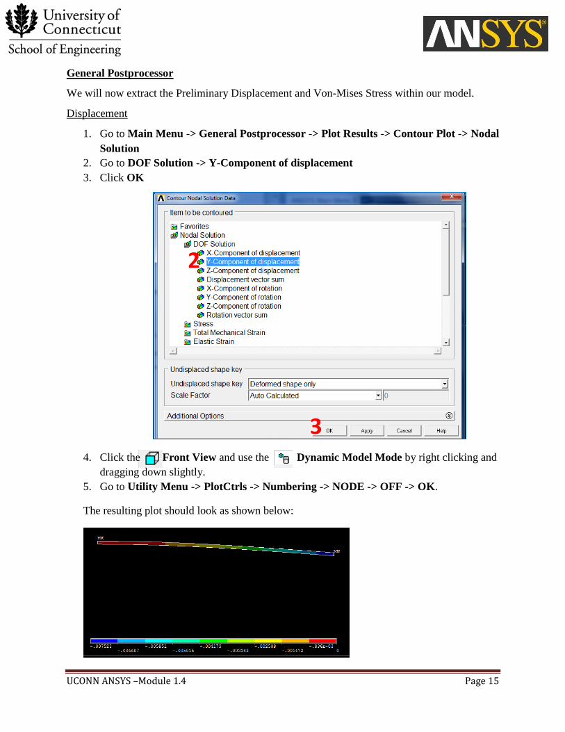
General Postprocessor

We will now extract the Preliminary Displacement and Von-Mises Stress within our model.

Displacement

1. Go to Main Menu -> General Postprocessor -> Plot Results -> Contour Plot -> Nodal

Solution

2. Go to DOF Solution -> Y-Component of displacement

3. Click OK

4. Click the Front View and use the Dynamic Model Mode by right clicking and

dragging down slightly.

5. Go to Utility Menu -> PlotCtrls -> Numbering -> NODE -> OFF -> OK.

The resulting plot should look as shown below:

2

3


Let’s change some plotting options and enhance the aesthetics.

6. Go to Utility Menu -> PlotCtrls -> Style ->

Contours -> Uniform Contours…

7. Under NCOUNT enter 9

8. Under Contour Intervals click

User Specified

9. Under VMIN enter -0.0075

The beam deflects in the –Y direction so

The max deflection is treated as a minimum

10. Under VMAX enter 0

11. Since we will be using 9 contour

intervals, we will enter 0.0075/9

for VINC

12. Click OK

13. Let’s give the plot a title. Go to Utility Menu -> Command Prompt and enter:

/title, Deflection of a Beam with an End Load and press enter

/replot and press enter

14. Let’s make the contour scheme go from red to dark blue instead of the current mapping.

Go to Utility Menu -> PlotCtrls -> Style -> Colors ->

Contour Colors …

15. Change Contour Number 1-9 to the colors below:

16. Click OK

The color bar should now read as below:

7

8

9-11

12

WARNING: Without considerable modifications to your

screen display drivers, ANSYS cannot display more than 9

contour bands.

15

16


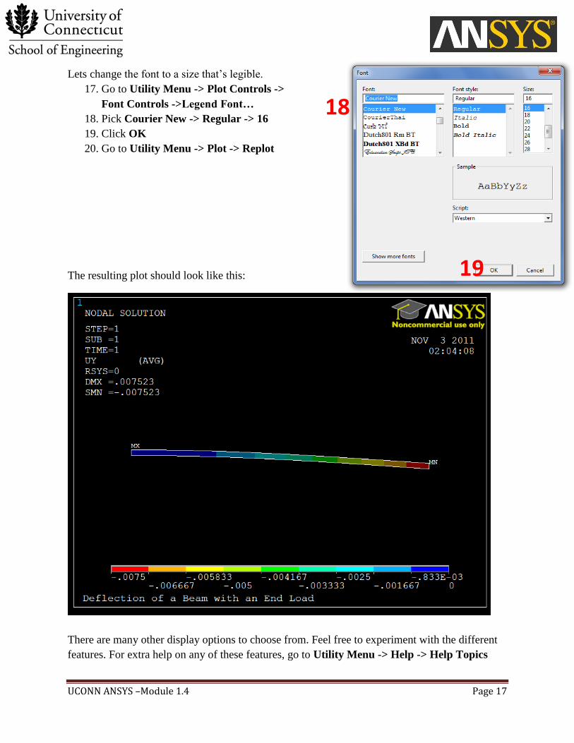
Lets change the font to a size that’s legible.

17. Go to Utility Menu -> Plot Controls ->

Font Controls ->Legend Font…

18. Pick Courier New -> Regular -> 16

19. Click OK


The resulting plot should look like this:

There are many other display options to choose from. Feel free to experiment with the different

features. For extra help on any of these features, go to Utility Menu -> Help -> Help Topics

18

19


Equivalent (Von-Mises) Stress

1. Go to Main Menu -> General Postprocessor -> Plot Results -> Contour Plot -> Nodal

Solution

2. Go to Nodal Solution -> Stress -> von Mises stress

3. Click OK

4. To get rid of the previous Plot Settings, go to

PlotCtrls -> Reset Plot Ctrls… and replot

5. Using the same methodology as the deflection plot, we can change the contour divisions

from 0 to 60000 in increments of 60000/9

6. Change the Title to “Von-Mises Stress of a Beam with a Point Load”


The resulting plot should look as below:


Results

Max Deflection Error

The percent error (%E) in our model max deflection can be defined as:

(

) = 1.14% (1.4.11)

This is a very good error baseline for the mesh considering eqation 1.4.9 is cubic with respect to

displacement. Since the 2D Elements we are using linearly interpolate between nodes, we can

expect a degree of truncation error in our model. As we will show in our validation section, our

model will converge to the expected solution as the mesh is refined.

Max Equivalent Stress Error

Using the same definition of error as before, we derive that our model has 9.43% error in the

max equivalent stress. Thus, it is reasonable that our choice of two elements through the width of

the beam is too coarse a mesh.

Further Analysis

In addition to this baseline data, we can export both the deflection and von-mises data to Excel.

1. Go to Utility Menu -> List -> Results -> Nodal Solution …

2. Select Nodal Solution -> DOF Solution -> Y-component of displacement

3. Click OK

4. The list file should populate. Go to

PRNSOL Command -> File -> Save As …

5. Save the file as 2D_P_YDeflection.lis to the

path of your choice

6. Go to PRNSOL Command -> File -> Close

4

5

6


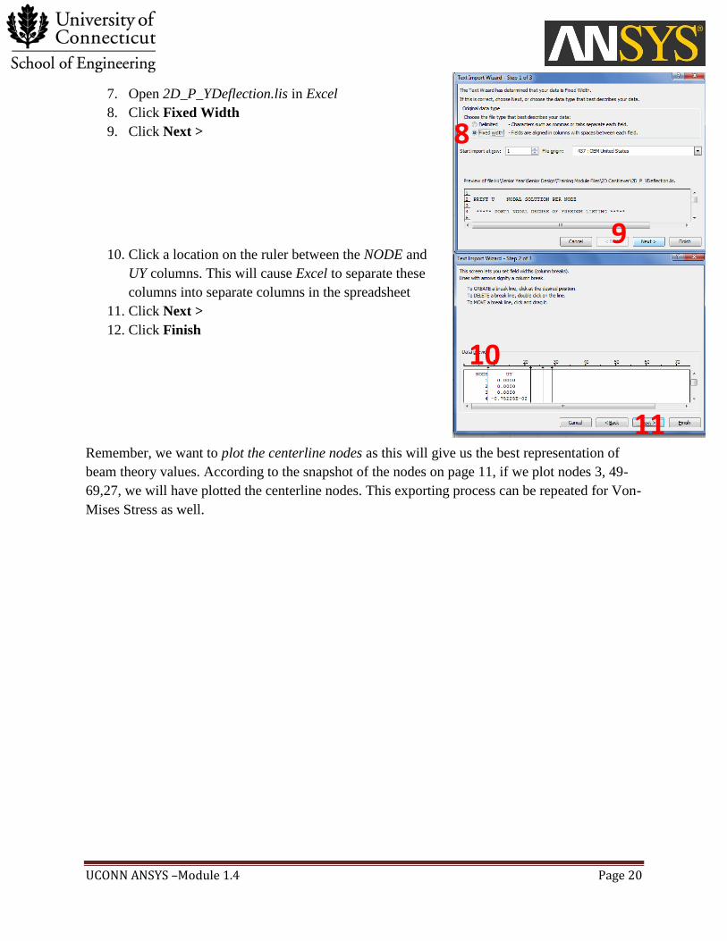
7. Open 2D_P_YDeflection.lis in Excel

8. Click Fixed Width

9. Click Next >

10. Click a location on the ruler between the NODE and

UY columns. This will cause Excel to separate these

columns into separate columns in the spreadsheet

11. Click Next >

12. Click Finish

Remember, we want to plot the centerline nodes as this will give us the best representation of

beam theory values. According to the snapshot of the nodes on page 11, if we plot nodes 3, 49-

69,27, we will have plotted the centerline nodes. This exporting process can be repeated for Von-

Mises Stress as well.

8

9

10

11


Validation

module 1.4: point loading of a 2d cantilever beam

Documents