module 03 modeling of dynamical systems

Physical Laws and Equations TF Models Mechanical System Model Electrical System Model Predator-Prey Model Linearization of NL Systems

Module 03Modeling of Dynamical Systems

Ahmad F. Taha

EE 3413: Analysis and Desgin of Control Systems

Email: [email protected]

Webpage: http://engineering.utsa.edu/˜taha

February 2, 2016

©Ahmad F. Taha Module 03 — Modeling of Dynamical Systems 1 / 26

http://engineering.utsa.edu/~taha


Module 3 Outline

1 Physical laws and equations2 Transfer function model3 Model of electrical systems4 Model of mechanical systems5 Examples

– Reading material: Dorf & Bishop, Section 2.3



Physical Laws and Models

By definition, dynamical systems are dynamic because they changewith time

Change in the sense that their intrinsic properties evolve, vary

Examples: coordinates of a drone, speed of a car, body temperature,concentrations of chemicals in a centrifuge

Physicists and engineers like to represent dynamic systems withequations

Why? Well, the answer is fairly straightforward

Dynamic model often means a differential equations



Physical Laws

For many systems, it’s easy to understand the physics, and hencethe math behind the physics

– Examples: circuits, motion of a cart, pendulum, suspension system

For the majority of dynamical systems, the actual physics is complex

Hence, it can be hard to depict the dynamics with ODEs

– Examples: human body temperature, thermodynamics, spacecrafts

This illustrates the needs for models

Dynamic system model: a mathematical description of the actualphysics



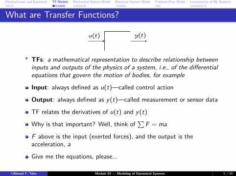
What are Transfer Functions?

* TFs: a mathematical representation to describe relationship betweeninputs and outputs of the physics of a system, i.e., of the differentialequations that govern the motion of bodies, for example

Input: always defined as u(t)—called control action

Output: always defined as y(t)—called measurement or sensor data

TF relates the derivatives of u(t) and y(t)

Why is that important? Well, think of∑

F = ma

F above is the input (exerted forces), and the output is theacceleration, a

Give me the equations, please...



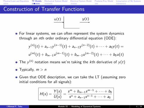
Construction of Transfer Functions

For linear systems, we can often represent the system dynamicsthrough an nth order ordinary differential equation (ODE):

y (n)(t) + an−1y (n−1)(t) + an−2y (n−2)(t) + · · ·+ a0y(t) =

u(m)(t) + bm−1u(m−1)(t) + bm−2u(m−2)(t) + · · ·+ b0u(t)

The y (k) notation means we’re taking the kth derivative of y(t)

Typically, m > n

Given that ODE description, we can take the LT (assuming zeroinitial conditions for all signals):

H(s) = Y (s)U(s) = sm + bm−1sm−1 + · · ·+ b0

sn + an−1sn−1 + · · ·+ a0



What are Transfer Functions?

Given this TF:

H(s) = Y (s)U(s) = sm + bm−1sm−1 + · · ·+ b0

sn + an−1sn−1 + · · ·+ a0

For a given control signal u(t) or U(s), we can find the output ofthe system, y(t), or Y (s)

Impulse response: defined as h(t)—the output y(t) if the inputu(t) = δ(t)

Step response: the output y(t) if the input u(t) = 1+(t)

For any input u(t), the output is: y(t) = h(t) ∗ u(t)

But...Convolutions are nasty...Who likes them?©Ahmad F. Taha Module 03 — Modeling of Dynamical Systems 7 / 26


TFs of Generic LTI Systems

So, we can take the Laplace transform: Y (s) = H(s)U(s)

Typically, we can write the TF as:

H(s) = Y (s)U(s) = sm + bm−1sm−1 + · · ·+ b0

sn + an−1sn−1 + · · ·+ a0

Roots of numerator are called the zeros of H(s) or the systemRoots of the denominator are called the poles of H(s)



Example

Given: H(s) = 2s + 1s3 − 4s2 + 6s − 4

Zeros: z1 = −0.5

Poles: solve s3 − 4s2 + 6s − 4 = 0, use MATLAB’s roots command

* poles=roots[1 -4 6 -4]; poles = {2, 1 + j , 1− j}

Factored form:

H(s) = 2 s + 0.5(s − 2)(s − 1− j)(s − 1 + j)



Analyzing Generic Physical SystemsSeven-step algorithm:

1 Identify dynamic variables, inputs (u), and system outputs (y)2 Focus on one component, analyze the dynamics (physics) of this

component

– How? Use Newton’s Equations, KVL, or thermodynamics laws...3 After that, obtain an nth order ODE:

n∑i=1

αi y (i)(t) =m∑

j=1βju(j)(t)

4 Take the Laplace transform of that ODE5 Combine the equations to eliminate internal variables6 Write the transfer function from input to output7 For a certain control U(s), find Y (s), then y(t) = L−1[Y (s)]



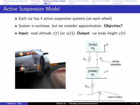
Active Suspension ModelEach car has 4 active suspension systems (on each wheel)

System is nonlinear, but we consider approximation. Objective?

Input: road altitude r(t) (or u(t)), Output: car body height y(t)



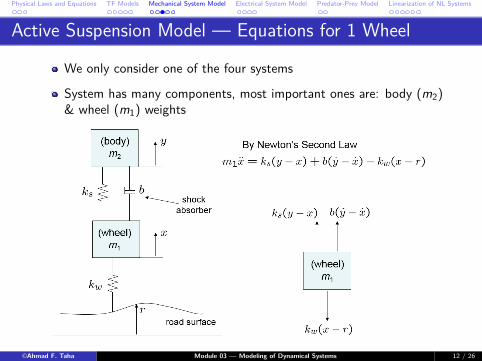
Active Suspension Model — Equations for 1 Wheel

We only consider one of the four systems

System has many components, most important ones are: body (m2)& wheel (m1) weights



Active Suspension Model — Equations for Car Body

We now have 2 equations depicting the car body and wheel motionObjective: find the TF relating output (y(t)) to input (r(t))

What is H(s) = Y (s)R(s) ?



Active Suspension Model — Transfer Function

Differential equations (in time):

m1x(t) = ks(y(t)− x(t)) + b(y(t)− x(t))− kw (x(t)− r(t))m2y(t) = −ks(y(t)− x(t))− b(y(t)− x(t))

Take Laplace transform given zero ICs:

– Solution:

Find H(s) = Y (s)R(s)

– Solution:



Basic Circuits Components



Basic Circuits — RLCs & Op-Amps



TF of an RLC Circuit — Example

Apply KVL (assume zero ICs):

vi(t) = Ri(t) + Ldi(t)dt + 1

C

∫i(τ)dt

vo(t) = 1C

∫i(τ)dt

Take LT for the above differential equations:

Vi(s) = RI(s) + LsI(s) + 1Cs I(s)

Vo(s) = 1Cs I(s) ⇒ I(s) = CsVo(s)

⇒ Vo(s)Vi(s) = 1

LCs2 + RCs + 1©Ahmad F. Taha Module 03 — Modeling of Dynamical Systems 17 / 26


Generic Circuit Analysis



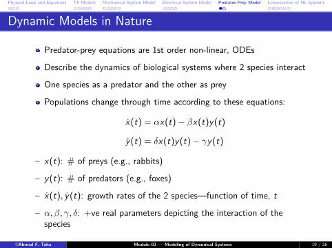
Dynamic Models in Nature

Predator-prey equations are 1st order non-linear, ODEs

Describe the dynamics of biological systems where 2 species interact

One species as a predator and the other as prey

Populations change through time according to these equations:

x(t) = αx(t)− βx(t)y(t)

y(t) = δx(t)y(t)− γy(t)

– x(t): # of preys (e.g., rabbits)

– y(t): # of predators (e.g., foxes)

– x(t), y(t): growth rates of the 2 species—function of time, t

– α, β, γ, δ: +ve real parameters depicting the interaction of thespecies



Mathematical Model

x(t) = αx(t)− βx(t)y(t)

y(t) = δx(t)y(t)− γy(t)

Prey’s population grows exponentially (αx(t))—why?

Rate of predation is assumed to be proportional to the rate at whichthe predators and the prey meet (βx(t)y(t))

If either x(t) or y(t) is zero then there can be no predation

δx(t)y(t) represents the growth of the predator population

No prey ⇒ no food for the predator ⇒ y(t) decays

Is there an equilibrium? What is it?



Nonlinear Dynamical Systems

Let’s face it: most dynamical systems are nonlinear

Nonlinearities can be seen in the ODEs, e.g.:

y(t) + y(t)y(t) + cos(y(t)) = 2u(t) + arctan(ecos(u(t)))

Examples: electromechanical systems, electronics, hydraulic systems,thermal, etc...

Why do we hate nonlinear systems?

– Well, because we cannot solve ODEs tractably if they are not linear

I mean we can, but they’re hard—and remember, we’re lazy

Solution: linearize nonlinear equations

Btw...most nonlinear systems are linear for a short period of time

So, it’s legit to linearize for a short period of time



Linearization — The Main IdeaLinearization is one of the most important techniques in controltheory

Without it, all our analysis of nonlinear systems becomes pointless

First, let’s assume that a nonlinear system is linearized around anoperating point

Operating point is often called equilibrium point

Main idea:



Linearization — The Simple Math

Nonlinear equation (or system): x(t) = f (x , u)

Equilibrium points: ue , xe

Equilibrium deviation : δu(t) = u(t)− ue , δx(t) = x(t)− xe

Taylor series expansion around ue , xe :

x(t) ≈ f (xe , ue) + (δx(t))∂f (x , u)∂x

∣∣∣∣xe ,ue

+ (δu(t))∂f (x , u)∂u

∣∣∣∣xe ,ue

Hence:

δx(t) ≈ (δx(t))∂f (x , u)∂x

∣∣∣∣xe ,ue

+ (δu(t))∂f (x , u)∂u

∣∣∣∣xe ,ue

This relationship is a linear one between δx and δu



Linearization — Example

Pendulum motion:

f (x , u) = −gL sin(x(t)) + 1

mL2 u(t)

x(t): angle (θ), u(t): force

Given equilibrium points: ue = 0, xe = π

Taylor series expansion around 0, π:

δf (δx , δu) ≈ gL δx(t) + 1

mL2 δu(t)

This relationship is a linear one between δx and δu: only valid in thevicinity of the equilibrium point



Roadmap Revisited



Questions And Suggestions?

Thank You!Please visit

engineering.utsa.edu/˜tahaIFF you want to know more ,


engineering.utsa.edu/~taha

module 03 modeling of dynamical systems

Documents