modeling and optimization of dynamical systems by
TRANSCRIPT
American Journal of Modeling and Optimization, 2016, Vol. 4, No. 1, 1-12 Available online at http://pubs.sciepub.com/ajmo/4/1/1 © Science and Education Publishing DOI:10.12691/ajmo-4-1-1
Modeling and Optimization of Dynamical Systems by Unconventional Spreadsheet Functions
Chahid Kamel Ghaddar*
ExcelWorks LLC, Sharon, MA, USA *Corresponding author: [email protected]
Abstract The spreadsheet computational engine is exploited via a nonstandard mechanism to support a functional formulation for constrained optimization of parameterized differential systems by unconventional spreadsheet functions. The nonstandard mechanism enables encapsulation of numerical algorithms into functions which take variable formulas as a new type of input argument while retaining purity and recursion properties. This is in contrast to conventional spreadsheet functions which are restricted to static input types. Several solvers for differential equations and nonlinear minimization are developed which serve as building blocks for the functional formulation. The latter makes it possible to express a program for a constrained dynamical minimization problem in as few as three formula evaluations in Excel as demonstrated by several examples. The solver functions integrate seamlessly with MS Excel, and propel the spreadsheet beyond traditional applications as a powerful tool for exploring dynamical optimization problems.
Keywords: dynamical optimization, optimal control, differential equations, spreadsheet, functional paradigm
Cite This Article: Chahid Kamel Ghaddar, “Modeling and Optimization of Dynamical Systems by Unconventional Spreadsheet Functions.” American Journal of Modeling and Optimization, vol.4, no. 1 (2016): 1-12.doi:10.12691/ajmo-4-1-1.
1. Introduction The spreadsheet inherent simplicity of defining formulas
and manipulating data, combined with rich intrinsic mathematical functions, graphing tools, and extensibility, have contributed to its widespread adoption in engineering and scientific applications [1,2,3]. Models for differential equations [4-10], optimization of algebraic and stochastic systems, and risk analysis [11,12] are well known. However, computational problems in constrained dynamical minimization involving systems of differential equations, and more generally optimal control problems, have remained beyond the utility of the spreadsheet. An example of such problems is computing optimal parameters for a differential equation system that minimize the sum of square errors for prescribed constraints on its response. The sought parameters may be any controls that influence the response of the system such as coefficients, forcing terms, boundary conditions, etc. Solving similar problems requires seamless integration of multiple solvers for constrained minimization and differential equations.
The standard design of the spreadsheet makes such an integration of solvers technically impractical. To point out the reasons, we briefly review the two distinct venues for adding functionality to a spreadsheet: Commands and Functions [13,14]. A command is the standard mechanism for evaluating formulas in the spreadsheet. MS Excel’s built in optimization solver is a good example of a command which works as follows:
1. The user selects cells to hold initial values for each decision variable in a model.
2. In another group of cells, the user defines formulas for the objective function and the left hand side of each constraint.
3. Via a command dialogue, the solver is executed which iterates, altering the decision cells values and recalculating the dependent objective and constraints cell values until such values are found which minimize the objective function value and satisfy the constraints.
Obviously, a command works by transforming its own inputs and does not behave as a proper mathematical function. It lacks the properties of purity, composition and could not support recursion. Differential equations solver extensions to Excel rely on commands, and operate in a similar fashion to the built in Excel solver, or may utilize the structured spreadsheet layout as a finite difference grid mixing up the input, algorithm and output [4-10]. Furthermore, a command cannot to be invoked programmatically as a re-usable function from other spreadsheet formulas [14]. Therefore, it is unfeasible to integrate multiple commands to solve a dynamical minimization problem.
On the other hand, the second mechanism for extending the spreadsheet utility is through the addition of new functions. The spreadsheet design permits only pure functions restricted to operating on constant inputs [13,14,15]. Some external programs, such as MATLAB [16] offer interfaces to Excel to expose a portion of their functionality. This model permits exchange of basic data types such as numbers, but cannot be used to expose differential and optimization solvers. Therefore, the standard spreadsheet functions could not either support a constrained minimization of a dynamical system.

2 American Journal of Modeling and Optimization
Certainly, the inherent design limitations of the spreadsheet unduly limit its full potential. Given the spreadsheet intuitive interface for defining formulas, it presents a practical platform for supporting native calculus solvers that could support a functional paradigm for dynamical optimization problems. Accordingly, the author has developed a method which overcomes the spreadsheet limitation and enables the creation of a first class function – function that can take other functions (i.e., formulas and variables) as arguments while preserving its mathematical properties including purity and recursion. Details of the method are provided in [17] and are rather technical in nature. However, the main idea is to capture the definition of an input formula via the spreadsheet Advanced Programming Interface (API) and construct a relational graph representing the formula inter-dependence on nested formulas, variable cells, and recursive calls. A graph evaluator which exploits the spreadsheet API evaluates the value of a formula without modifying any data in the spreadsheet.
The flowchart logic for developing a first class solver is shown in Figure 1. The benefits gained by enabling a first class solver in the spreadsheet are noteworthy. The spreadsheet’s computational engine could be exploited to support intrinsic solvers for virtually any system that can be modelled by formulas and variables [18]. For example, the flow chart of Figure 1 makes possible, for the first time, the existence of the following intrinsic worksheet integration function:
( , , , , [ ])QUADF f x a b Options= (1)
for computing a formula integral ( )ba
f x dx∫ using
appropriate algorithms [19].
Figure 1. Flow chart for unconventional first class spreadsheet function design
Table 1 illustrates utilizing (1) to compute the integral
of 10
ln 4xdxx
= −∫ in Excel. The reference to the integrand
formula A1 1, the variable of integration X1, and limits are passed to (1) as regular parameters. Evaluating QUADF formula in A2 computes the results without any side effects. Such a practical integration function has never existed in a spreadsheet application before.
Table 1. Computing a formula integral in Excel by the worksheet function (1)
A A
1 =LN(X1)/SQRT(X1) 1 #NUM!
2 =QUADF(A1,X1,0,1) 2 -4
More importantly, by preserving function properties including purity and recursion, the first class solvers can be utilized as building blocks of a functional paradigm for solving dynamical optimization problems. A simple example of a functional program is illustrated in Table 2 in which (1) is employed to compute the volume integral
32 3 6 3 22
0 0 01 3.
x x yxdzdydx
− − −− =∫ ∫ ∫ Here each inner
QUADF formula serves as the integrand for the next outer QUADF formula. Evaluating the outer integral in A4 computes the triple integral value.
Table 2. Example of using recursion to compute triple integral in Excel A A
1 =1-X1 1 1
2 =QUADF(A1,Z1,0,6-3*X1-2*Y1) 2 6
3 =QUADF(A2,Y1,0,3-3*X1/2) 3 9
4 =QUADF(A3,X1,0,2) 4 3
In Section 2 we present an abstract functional formulation which permits us to utilize first class spreadsheet functions to solve constrained dynamical minimization problems in Excel. The formulation is motivated by the combination of the benefits of a functional programming paradigm [20] with the simplicity of using the spreadsheet application. It enables expressing the solution steps from an engineering view point, rather than describe the computational logic in a procedural style, as is commonly practiced. Given a set of control parameters, we model and obtain an initial response of the differential system based on initial values for the control parameters. In the next step, we state design objectives in the form of constraint formulas, which penalize the deviation of the initial response from a desired target response. Finally, we compute values for the control parameters to minimize the sum of squared errors in the set of design constraints. These steps map directly to three classes of first class functions: solvers for differential equation systems; criterion functions to enable definition of dynamical constraints on a system response; and a functional minimizer for the set of constraints. As shall be demonstrated in the examples, it is possible to express a
1The #NUM! error reported by Excel is due to division by X1 which is undefined. X1 is chosen as a dummy variable for the formula. Its value, assumed zero by Excel, is irrelevant, and the error can be ignored.

American Journal of Modeling and Optimization 3
program for constrained minimization in as few as three function evaluations in Excel.
The three classes of functions which form the building blocks of the functional formulation are presented in the following section with full description provided in Appendices A-C. Section 3 presents three examples employing the spreadsheet functions for solving the following constrained optimization problems: • Computing the required thrust and arrival time for a
travelling train. • Customizing a second order dynamical system. • Controlling heat transfer across a slab. We note that this article primary focus is to introduce
and illustrate the solution framework using pedagogical examples rather than analyze any specific physical problem. In addition, the article does not review other non-spreadsheet methods, but leave it to the reader to withdraw own conclusion on the merits of the presented approach in comparison to other familiar mathematical software. Finally, we recommend reviewing Appendix A which includes a brief description of basic spreadsheet concepts for any reader not familiar with the spreadsheet.
2. Functional Formulation for the Dynamical Optimization Problem
In the following, we present a functional formulation for the constrained minimization problem which is based on first class spreadsheet solvers. In what follows, a bold symbol indicates a vector value. Let 𝒖(𝑥,𝒑𝒅) be the solution function to a system of differential equations where 𝑥 is an independent variable and 𝒑𝒅 is a set of design parameters that influence the system response. 𝒖(𝑥,𝒑𝒅) can be interpreted as a solution function returned by a higher order solver function [20] for the differential equations system. The solution function provides values for the differential system variables 𝒖 = [𝑢1,𝑢2, . . ,𝑢𝑛] at a specified value for the independent variable , 𝑥, and for a given configuration of the system design parameters, 𝒑𝒅. In a spreadsheet context, 𝒖(𝑥,𝒑𝒅) represents an abstract tabular result value of a differential equation system solver.
Let 𝑓𝑖(𝒖(𝑥,𝒑𝒅), [𝑥],𝒑𝒅) be a criterion functional that computes a scalar property of interest from the differential system response, 𝒖(𝑥,𝒑𝒅) , for a specified range of the independent variable, [𝑥] , and specified values for the design parameters, 𝒑𝒅 . For example, 𝑓𝑖 may simply extract a single value from 𝒖(𝑥,𝒑𝒅), or may compute a complex property by applying a prescribed operation, such as integrating a component of 𝒖(𝑥,𝒑𝒅) over a specified range [𝑥] . Given a target design value, 𝜏𝑖 , for each criterion functional, 𝑓𝑖, we construct the following ordered system of 𝑚 constraints:
( )( )
0, 1,..,
0, 1,..,i
j
g i k
g j k m
= =
≥ = +d
d
p
p (2)
where 𝑔𝑖 , 𝑖 = 1, . . ,𝑚 is a suitable penalty functional which may take the simple form:
( ) ( ) [ ]( ), , , ,i i ig f x x τ≡ −d d dp u p p (3)
Let:
( ) ( )0, 0
1,j
jif g is ture
elseδ
≥=
dd
pp (4)
for 𝑗 = 𝑘 + 1, . . ,𝑚, be an indicator weight function which takes on the value one for each active (unsatisfied) inequality constraint, or zero otherwise.
Accordingly, the optimal design parameters values we seek to compute, minimize the following implicit cost functional:
( ) ( ) ( ) ( ) 22
1 1i j jC g g δ
= = +
= + ∑ ∑k m
d d d di j k
p p p p (5)
Based on the flowchart of Figure 1, in conjunction with a suitable minimization algorithm such as the Levenberg-Marquardt algorithm [21,22], the minimization of the objective (5) can be practically expressed in the spreadsheet by the evaluation of a worksheet functional minimizer solver of the form:
( )( , ,[ ])solve m k= −d d g p p (6)
which takes the vector of constraint formulas, design variables, and the number of inequality constraints, 𝑚− 𝑘. The functional formulation ensures that evaluation of a criterion constraint formula by the solver algorithm triggers re-evaluation of the underling dynamical system in order to compute a current value for the constraint at any given values of the design parameters [17].
We remark that although the above formulation does not specify an explicit general cost functional, it is easily amenable to incorporating one. Such a modification would entail: modifying the solver (6) interface to accept an additional cost formula, 𝐺(𝒑𝒅) , and updating the underlining solver algorithm. Expanding the framework to support an explicit cost functional including continuous time cost functional for optimal control problems [23] will be addressed in a forthcoming effort.
The abstract functional formulation (2)-(6) lays the foundation for a practical three-step dynamical optimization process that can be carried out using three type of pure spreadsheet functions which we described next.
2.1. Differential Equations Solvers Two spreadsheet solvers, IVSOLVE() and BVSOLVE()
suitable for initial and boundary value problems, have been developed and described in Appendix A. To utilize the solvers, the differential system must be presented as a set of first order equations
( ), , , 1,..,ii
duf x i n
dx= =du p (7)
which are easily modelled in a spreadsheet by the system RHS formulas (𝑓1, 𝑓2, . . , 𝑓𝑛). These formulas are passed as arguments to the solvers along with the system variables (𝑥,𝑢1,𝑢2, . . ,𝑢𝑛) , as detailed in Appendix A. The 3rd solver, PDSOLVE(), suitable for initial-boundary value partial differential problems is also presented in Appendix A, and utilized in Example 3.3.
A solver is executed as a regular intrinsic array formula in an allocated range of the spreadsheet. The solver computes and displays a formatted result as shown in

4 American Journal of Modeling and Optimization
Figure 2. The result table serves as a discrete proxy for the function 𝒖(𝑥,𝒑𝒅) in (2)-(6) providing a map between the independent variable 𝑥 and the state variables 𝒖 for specified values of the design parameters 𝒑𝒅.
Figure 2. Solution layout in Excel for differential systems solvers IVSOLVE() and BVSOLVE()
2.2. Criterion Functions A criterion function corresponds to 𝑓𝑖(𝒖(𝑥,𝒑𝒅), [𝑥],𝒑𝒅)
in (3), and computes a scalar property from the solution array (see Figure 2) of a differential systems solver for the purpose of constraining the response. A constraint formula penalizes the difference between the computed scalar property value and a target value. In essence, the criterion function provides the dynamical link that connects the differential systems solver with the functional minimizer and enables the operation of the functional formulation (2)-(6). The dynamical links are achieved naturally such that evaluation of a constraint formula leads to re-evaluation of the underling differential solver [17] in order to compute a current value for the scalar property of interest.
The scalar property may be a direct value extracted from the solution at a specified point, or an indirect computed value utilizing a prescribed calculus operation or a user defined formula. To accommodate general applications, two criterion functions, ARRAYVAL() and ODEVAL(), have been developed and described in Appendix B. ARRAYVAL() applies user-defined formulas to map a selected data set within the solution array (Figure 2) to a scalar value. On the other hand, ODEVAL() applies a calculus operation, such as differentiation or interpolation, to compute a value from the solution array. We remark that the parameter differences between the abstract criterion functional and the actual implementations described in Appendix B are rather a technical exploitation of the spreadsheet and functional programming properties, which permit us to assign and recover functions from variables [17].
2.3. Functional Minimizer A functional minimizer NLSOLVE(), which
corresponds to (6), is described in Appendix C. It receives the set of formula constraints, and design parameters variables, and computes optimal values for the latter that minimize the implicit cost functional (5).
The aforementioned spreadsheet functions enable the three-step optimization formulation (2)-(6) comprising the following practical steps.
I. Using initial values of the design parameters, obtain an initial response to the parameterized differential
system by a suitable solver IVSOLVE(), BVSOLVE(), or PDSOLVE().
II. Define constraints on the initial system response using the criterion functions ARRAYVAL() and ODEVAL().
III. Solve for the set of constraints for the optimal design parameters using NLSOLVE().
These steps are demonstrated in the following section with three examples in Excel.
3. Constrained Optimization Examples
3.1. Travelling Train Problem In this example we compute the required propulsion
force and the travel time for a frictionless train travelling between two cities through a straight tunnel. The train uses a constant propulsion force to accelerate, but relies solely on the gravitational pull of the Earth, as well as aerodynamic drag, for deceleration. Using the assumptions shown in Table 3 and referring to Figure 3, we formulate the problem as a constrained optimization problem as follows.
Figure 3 shows the forces acting on the train during its trip from City A to City B along the circular path of the earth. The motion for the train is governed by the second order equation:
( ) ( ( ))t p d gm x F F x F xθ= − + (8)
with the initial conditions 𝑥(0) = 0, �̇�(0) = 0 at departure City A.
Table 3. Assumptions and parameters for problem 3.1 Train mass 𝑚𝑡 = 100,000 (kg) Distance travelled 𝑑 = 1000,000 (m) Earth Radius 𝑅 = 6371,000 (m) Gravitational constant 𝑔 = 10 𝑚/𝑠2 Drag force 𝐹𝑑(𝑣) = 0.5 ∗ 𝑣2 (N) Propulsion force 𝐹𝑝= constant (N) Gravitational force 𝐹𝑔(𝜃) = 𝑚𝑡 ∗ 𝑔 ∗ cos (𝜃) (N)
Figure 3. Schematic for the forces acting on the travelling train of problem 3.1
Using 𝑑/𝑅 ≪ 1, the angle of rotation, 𝜃, (see Figure 3) can be approximated by the following formula:
( )
1
1
tan , / 2/ 2
, / 22
tan , / 2/ 2
R x dd x
x x d
R x dd x
πθ
π
−
−
< −
= = + > −
(9)
American Journal of Modeling and Optimization 5
On arrival at City B, the train comes to a halt, so the final conditions can be stated as:
( )( ) 0
f
f
x t d
x t
=
=
(10)
The final conditions (10) can be viewed as constraints on the differential equation (8) for the train’s motion. The problem is thus reduced to finding optimal values for the unknown propulsion force 𝐹𝑝 and the travel time 𝑡𝑓 such that the two constraints (10) are satisfied. We compute the answer by a simple functional program in Excel spreadsheet corresponding to the three-step optimization process as shown below.
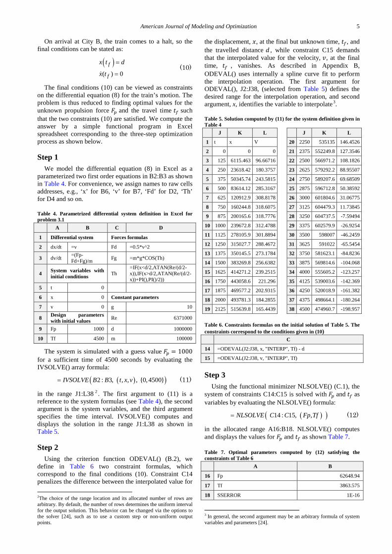
Step 1 We model the differential equation (8) in Excel as a
parameterized two first order equations in B2:B3 as shown in Table 4. For convenience, we assign names to raw cells addresses, e.g., ‘x’ for B6, ‘v’ for B7, ‘Fd’ for D2, ‘Th’ for D4 and so on.
Table 4. Parametrized differential system definition in Excel for problem 3.1
A B C D
1 Differential system Forces formulas
2 dx/dt =v Fd =0.5*v^2
3 dv/dt =(Fp-Fd+Fg)/m Fg =m*g*COS(Th)
4 System variables with initial conditions Th
=IF(x<d/2,ATAN(Re/(d/2-x)),IF(x>d/2,ATAN(Re/(d/2-x))+PI(),PI()/2))
5 t 0 6 x 0 Constant parameters
7 v 0 g 10
8 Design parameters with initial values Re 6371000
9 Fp 1000 d 1000000
10 Tf 4500 m 100000
The system is simulated with a guess value 𝐹𝑝 = 1000 for a sufficient time of 4500 seconds by evaluating the IVSOLVE() array formula:
( )( )2 : 3, , , , {0,4500}IVSOLVE B B t x v= (11)
in the range J1:L38 2 . The first argument to (11) is a reference to the system formulas (see Table 4), the second argument is the system variables, and the third argument specifies the time interval. IVSOLVE() computes and displays the solution in the range J1:L38 as shown in Table 5.
Step 2 Using the criterion function ODEVAL() (B.2), we
define in Table 6 two constraint formulas, which correspond to the final conditions (10). Constraint C14 penalizes the difference between the interpolated value for 2The choice of the range location and its allocated number of rows are arbitrary. By default, the number of rows determines the uniform interval for the output solution. This behavior can be changed via the options to the solver [24], such as to use a custom step or non-uniform output points.
the displacement, 𝑥, at the final but unknown time, 𝑡𝑓, and the travelled distance 𝑑 , while constraint C15 demands that the interpolated value for the velocity, 𝑣, at the final time, 𝑡𝑓 , vanishes. As described in Appendix B, ODEVAL() uses internally a spline curve fit to perform the interpolation operation. The first argument for ODEVAL(), J2:J38, (selected from Table 5) defines the desired range for the interpolation operation, and second argument, x, identifies the variable to interpolate3.
Table 5. Solution computed by (11) for the system definition given in Table 4
J K L J K L
1 t x V 20 2250 535135 146.4526
2 0 0 0 21 2375 552249.8 127.3546
3 125 6115.463 96.66716 22 2500 566971.2 108.1826
4 250 23618.42 180.3757 23 2625 579292.2 88.95507
5 375 50345.74 243.5815 24 2750 589207.6 69.68509
6 500 83614.12 285.3167 25 2875 596712.8 50.38592
7 625 120912.9 308.8178 26 3000 601804.6 31.06775
8 750 160244.8 318.6075 27 3125 604479.3 11.73845
9 875 200165.6 318.7776 28 3250 604737.5 -7.59494
10 1000 239672.8 312.4788 29 3375 602579.9 -26.9254
11 1125 278105.9 301.8894 30 3500 598007 -46.2459
12 1250 315027.7 288.4672 31 3625 591022 -65.5454
13 1375 350145.5 273.1784 32 3750 581623.1 -84.8236
14 1500 383269.8 256.6382 33 3875 569814.6 -104.068
15 1625 414271.2 239.2515 34 4000 555605.2 -123.257
16 1750 443058.6 221.296 35 4125 539003.6 -142.369
17 1875 469577.2 202.9315 36 4250 520018.9 -161.382
18 2000 493781.3 184.2855 37 4375 498664.1 -180.264
19 2125 515639.8 165.4439 38 4500 474960.7 -198.957
Table 6. Constraints formulas on the initial solution of Table 5. The constraints correspond to the conditions given in (10)
C
14 =ODEVAL(J2:J38, x, "INTERP", Tf) - d
15 =ODEVAL(J2:J38, v, "INTERP", Tf)
Step 3 Using the functional minimizer NLSOLVE() (C.1), the
system of constraints C14:C15 is solved with 𝐹𝑝 and 𝑡𝑓 as variables by evaluating the NLSOLVE() formula:
( )( ) 14 : 15, , NLSOLVE C C Fp Tf= (12)
in the allocated range A16:B18. NLSOLVE() computes and displays the values for 𝐹𝑝 and 𝑡𝑓 as shown Table 7.
Table 7. Optimal parameters computed by (12) satisfying the constraints of Table 6
A B
16 Fp 62648.94
17 Tf 3863.575
18 SSERROR 1E-16
3 In general, the second argument may be an arbitrary formula of system variables and parameters [24].
6 American Journal of Modeling and Optimization
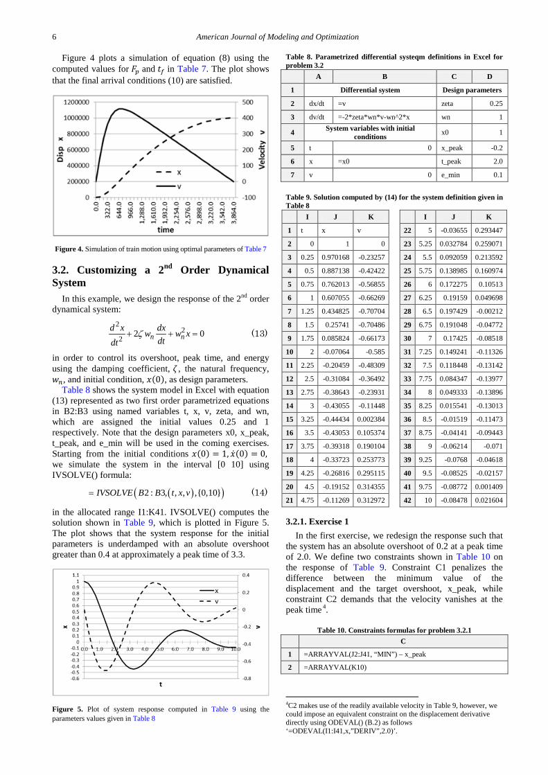
Figure 4 plots a simulation of equation (8) using the computed values for 𝐹𝑝 and 𝑡𝑓 in Table 7. The plot shows that the final arrival conditions (10) are satisfied.
Figure 4. Simulation of train motion using optimal parameters of Table 7
3.2. Customizing a 2nd Order Dynamical System
In this example, we design the response of the 2nd order dynamical system:
2
22 2 0n n
d x dxw w xdtdt
ζ+ + = (13)
in order to control its overshoot, peak time, and energy using the damping coefficient, 𝜁 , the natural frequency, 𝑤𝑛, and initial condition, 𝑥(0), as design parameters.
Table 8 shows the system model in Excel with equation (13) represented as two first order parametrized equations in B2:B3 using named variables t, x, v, zeta, and wn, which are assigned the initial values 0.25 and 1 respectively. Note that the design parameters x0, x_peak, t_peak, and e_min will be used in the coming exercises. Starting from the initial conditions 𝑥(0) = 1, �̇�(0) = 0, we simulate the system in the interval [0 10] using IVSOLVE() formula:
( )( )2 : 3, , , ,{0,10}IVSOLVE B B t x v= (14)
in the allocated range I1:K41. IVSOLVE() computes the solution shown in Table 9, which is plotted in Figure 5. The plot shows that the system response for the initial parameters is underdamped with an absolute overshoot greater than 0.4 at approximately a peak time of 3.3.
Figure 5. Plot of system response computed in Table 9 using the parameters values given in Table 8
Table 8. Parametrized differential systeqm definitions in Excel for problem 3.2
A B C D
1 Differential system Design parameters
2 dx/dt =v zeta 0.25
3 dv/dt =-2*zeta*wn*v-wn^2*x wn 1
4 System variables with initial conditions x0 1
5 t 0 x_peak -0.2
6 x =x0 t_peak 2.0
7 v 0 e_min 0.1
Table 9. Solution computed by (14) for the system definition given in Table 8 I J K I J K
1 t x v 22 5 -0.03655 0.293447
2 0 1 0 23 5.25 0.032784 0.259071
3 0.25 0.970168 -0.23257 24 5.5 0.092059 0.213592
4 0.5 0.887138 -0.42422 25 5.75 0.138985 0.160974
5 0.75 0.762013 -0.56855 26 6 0.172275 0.10513
6 1 0.607055 -0.66269 27 6.25 0.19159 0.049698
7 1.25 0.434825 -0.70704 28 6.5 0.197429 -0.00212
8 1.5 0.25741 -0.70486 29 6.75 0.191048 -0.04772
9 1.75 0.085824 -0.66173 30 7 0.17425 -0.08518
10 2 -0.07064 -0.585 31 7.25 0.149241 -0.11326
11 2.25 -0.20459 -0.48309 32 7.5 0.118448 -0.13142
12 2.5 -0.31084 -0.36492 33 7.75 0.084347 -0.13977
13 2.75 -0.38643 -0.23931 34 8 0.049333 -0.13896
14 3 -0.43055 -0.11448 35 8.25 0.015541 -0.13013
15 3.25 -0.44434 0.002384 36 8.5 -0.01519 -0.11473
16 3.5 -0.43053 0.105374 37 8.75 -0.04141 -0.09443
17 3.75 -0.39318 0.190104 38 9 -0.06214 -0.071
18 4 -0.33723 0.253773 39 9.25 -0.0768 -0.04618
19 4.25 -0.26816 0.295115 40 9.5 -0.08525 -0.02157
20 4.5 -0.19152 0.314355 41 9.75 -0.08772 0.001409
21 4.75 -0.11269 0.312972 42 10 -0.08478 0.021604
3.2.1. Exercise 1 In the first exercise, we redesign the response such that
the system has an absolute overshoot of 0.2 at a peak time of 2.0. We define two constraints shown in Table 10 on the response of Table 9. Constraint C1 penalizes the difference between the minimum value of the displacement and the target overshoot, x_peak, while constraint C2 demands that the velocity vanishes at the peak time 4.
Table 10. Constraints formulas for problem 3.2.1
C
1 =ARRAYVAL(J2:J41, “MIN”) – x_peak
2 =ARRAYVAL(K10)
4C2 makes use of the readily available velocity in Table 9, however, we could impose an equivalent constraint on the displacement derivative directly using ODEVAL() (B.2) as follows ‘=ODEVAL(I1:I41,x,”DERIV”,2.0)’.

American Journal of Modeling and Optimization 7
The system of constraints C1:C2 is solved with 𝑤𝑛 and 𝜁 as variables by evaluating the functional minimizer NLSOLVE() formula:
( ) ( )( ) 1, 2 , , NLSOLVE C C zeta wn= (15)
in allocated range D1:E3. NLSOLVE() computes the results shown Table 11. Figure 6 shows the modified system response using the values for 𝑤𝑛 and 𝜁 of Table 11.
Table 11. Optimal parameters computed by (15) satisfying constraints of Table 10
D E
1 zeta 0.451081913
2 wn 1.659599536
3 SSERROR 2.20497E-26
Figure 6. Modified system response using optimal parameters of Table 11
For illustration, we solve the same system of constraints in Table 10, but with initial displacement, x0, and 𝑤𝑛 as design variables. Here we simply need to replace zeta with x0, and evaluate the new NLSOLVE() formula:
( ) ( )( )1, 2 , 0,NLSOLVE C C x wn= (16)
The results are shown in Table 12 and plotted in Figure 7. As expected, the solution satisfies the constraints, but retains the underdamped behavior of the system.
Table 12. Optimal parameters computed by (16) satisfying constraints of Table 10
D E
1 x0 0.450161581
2 wn 1.622267731
3 SSERROR 1.08134E-11
Figure 7. Modified system response using parameters of Table 12
3.2.2. Exercise 2 In this exercise we constrain the absolute overshoot,
and the minimal available energy at the unknown peak time, 𝑡𝑝 , then compute the damping coefficient, 𝜁 , the natural frequency, 𝑤𝑛 , and the attained peak time, 𝑡𝑝. At the overshoot, the velocity is zero and the total energy is defined by:
2 *ne w x= (17)
The constraints are stated as follows:
( )( )
( )
_ 0
0
_ 0
p
p
p
x t x peak
v t
e t e min
− =
=
− ≥
(18)
where𝑥_𝑝𝑒𝑎𝑘 and 𝑒_𝑚𝑖𝑛 values are specified in Table 8. Table 13 shows the equivalent Excel constraints defined on the initial solution of Table 9 by aid of the criterion function ODEVAL() which uses interpolation to compute the values at the variable t_peak.
Table 13. Constraints formulas for problem 3.2- Exercise 2
C 4 =ODEVAL(I2:I41, x, ”INTERP”, t_peak) – x_peak 5 =ODEVAL(I2:I41, v, ”INTERP”, t_peak) 6 =wn*ODEVAL(I2:I41, x, ”INTERP”, t_peak)^2 – e_min
The system of constraints C4:C6 is solved by NLSOLVE() formula:
( ) ( )( ) 4, 6 , , , _ , 1NLSOLVE C C zeta wn t peak= (19)
in the allocated range F1:G3 shown in Table 14. Note that we pass one in the third argument to indicate the last constraint is an inequality constraint. Figure 8 shows the modified system response using the computed values for 𝜁 and 𝑤𝑛 which shows the peak time occurs near 1.4.
Table 14. Optimal parameters computed by (19) satisfying the constraints of Table 13
F G 1 zeta 0.455927572 2 wn 2.5 3 t_peak 1.412086279 4 SSERROR 1.08134E-11
Figure 8. Modified system response using parameters of Table 14
3.3. Heat Transfer Problem In this example, we demonstrate how to setup a simple
functional program to control a heat transfer problem. We
8 American Journal of Modeling and Optimization
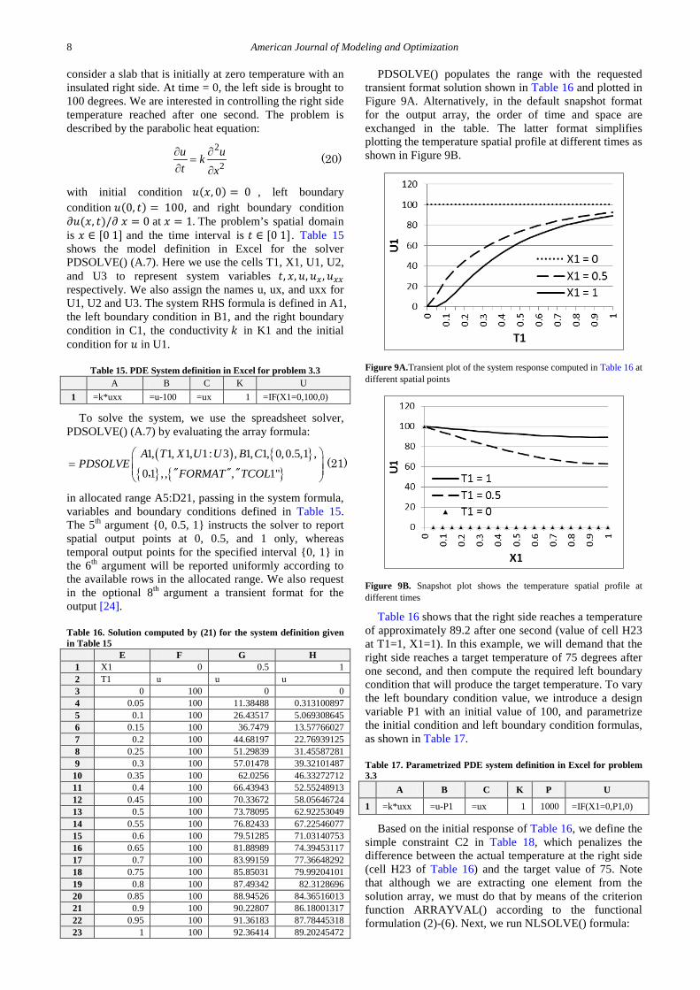
consider a slab that is initially at zero temperature with an insulated right side. At time = 0, the left side is brought to 100 degrees. We are interested in controlling the right side temperature reached after one second. The problem is described by the parabolic heat equation:
2
2u ukt x
∂ ∂=
∂ ∂ (20)
with initial condition 𝑢(𝑥, 0) = 0 , left boundary condition 𝑢(0, 𝑡) = 100, and right boundary condition 𝜕𝑢(𝑥, 𝑡)/𝜕 𝑥 = 0 at 𝑥 = 1. The problem’s spatial domain is 𝑥 ∈ [0 1] and the time interval is 𝑡 ∈ [0 1]. Table 15 shows the model definition in Excel for the solver PDSOLVE() (A.7). Here we use the cells T1, X1, U1, U2, and U3 to represent system variables 𝑡, 𝑥,𝑢,𝑢𝑥 ,𝑢𝑥𝑥 respectively. We also assign the names u, ux, and uxx for U1, U2 and U3. The system RHS formula is defined in A1, the left boundary condition in B1, and the right boundary condition in C1, the conductivity 𝑘 in K1 and the initial condition for 𝑢 in U1.
Table 15. PDE System definition in Excel for problem 3.3
A B C K U 1 =k*uxx =u-100 =ux 1 =IF(X1=0,100,0)
To solve the system, we use the spreadsheet solver, PDSOLVE() (A.7) by evaluating the array formula:
( ) { }{ } { } 1, 1, 1, 1: 3 , 1, 1, 0,0.5,1 ,
0 1 , , , 1"
A T X U U B CPDSOLVE
FORMAT TCOL
=
, " " "(21)
in allocated range A5:D21, passing in the system formula, variables and boundary conditions defined in Table 15. The 5th argument {0, 0.5, 1} instructs the solver to report spatial output points at 0, 0.5, and 1 only, whereas temporal output points for the specified interval {0, 1} in the 6th argument will be reported uniformly according to the available rows in the allocated range. We also request in the optional 8th argument a transient format for the output [24].
Table 16. Solution computed by (21) for the system definition given in Table 15
E F G H 1 X1 0 0.5 1 2 T1 u u u 3 0 100 0 0 4 0.05 100 11.38488 0.313100897 5 0.1 100 26.43517 5.069308645 6 0.15 100 36.7479 13.57766027 7 0.2 100 44.68197 22.76939125 8 0.25 100 51.29839 31.45587281 9 0.3 100 57.01478 39.32101487
10 0.35 100 62.0256 46.33272712 11 0.4 100 66.43943 52.55248913 12 0.45 100 70.33672 58.05646724 13 0.5 100 73.78095 62.92253049 14 0.55 100 76.82433 67.22546077 15 0.6 100 79.51285 71.03140753 16 0.65 100 81.88989 74.39453117 17 0.7 100 83.99159 77.36648292 18 0.75 100 85.85031 79.99204101 19 0.8 100 87.49342 82.3128696 20 0.85 100 88.94526 84.36516013 21 0.9 100 90.22807 86.18001317 22 0.95 100 91.36183 87.78445318 23 1 100 92.36414 89.20245472
PDSOLVE() populates the range with the requested transient format solution shown in Table 16 and plotted in Figure 9A. Alternatively, in the default snapshot format for the output array, the order of time and space are exchanged in the table. The latter format simplifies plotting the temperature spatial profile at different times as shown in Figure 9B.
Figure 9A.Transient plot of the system response computed in Table 16 at different spatial points
Figure 9B. Snapshot plot shows the temperature spatial profile at different times
Table 16 shows that the right side reaches a temperature of approximately 89.2 after one second (value of cell H23 at T1=1, X1=1). In this example, we will demand that the right side reaches a target temperature of 75 degrees after one second, and then compute the required left boundary condition that will produce the target temperature. To vary the left boundary condition value, we introduce a design variable P1 with an initial value of 100, and parametrize the initial condition and left boundary condition formulas, as shown in Table 17.
Table 17. Parametrized PDE system definition in Excel for problem 3.3
A B C K P U
1 =k*uxx =u-P1 =ux 1 1000 =IF(X1=0,P1,0)
Based on the initial response of Table 16, we define the simple constraint C2 in Table 18, which penalizes the difference between the actual temperature at the right side (cell H23 of Table 16) and the target value of 75. Note that although we are extracting one element from the solution array, we must do that by means of the criterion function ARRAYVAL() according to the functional formulation (2)-(6). Next, we run NLSOLVE() formula:
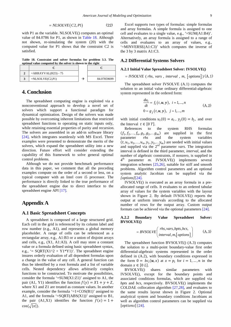
American Journal of Modeling and Optimization 9
( )2, 1NLSOLVE C P= (22)
with P1 as the variable. NLSOLVE() computes an optimal value of 84.0786 for P1, as shown in Table 18. Although not shown, re-simulating the system (20) with the computed value for P1 shows that the constraint C2 is satisfied.
Table 18. Constraint and solver formulas for problem 3.3. The optimal value computed by the solver is shown to the right
C C
2 =ARRAYVAL(H23) - 75 3 =NLSOLVE(C2,P1) 84.07859699
4. Conclusion The spreadsheet computing engine is exploited via a
nonconventional approach to develop a novel set of solvers which support a functional paradigm for dynamical optimization. Design of the solvers was made possible by overcoming inherent limitations that restricted spreadsheet functions to operating on static inputs only, while retaining essential properties of purity and recursion. The solvers are assembled in an add-in software library [24], which integrates seamlessly with MS Excel. Three examples were presented to demonstrate the merits of the solvers, which expand the spreadsheet utility into a new direction. Future effort will consider extending the capability of this framework to solve general optimal control problems.
Although we do not provide benchmark performance data in this paper, we comment that all the preceding examples compute on the order of a second or less, on a typical computer with an Intel core i5 processor. The performance is directly linked to the true performance of the spreadsheet engine due to direct interface to the spreadsheet engine API [17].
Appendix A
A.1 Basic Spreadsheet Concepts A spreadsheet is composed of a large structured grid.
Each cell in the grid is referenced by its column label and row number (e.g., A1), and represents a global memory placeholder. A range of cells can be referenced as a rectangular array, e.g., A1:B3 or a union of disjoint arrays and cells, e.g., (X1, A1:A3). A cell may store a constant value or a formula defined using basic spreadsheet syntax, e.g., ‘= SQRT(X1^2 + Y1*Y1)’. The spreadsheet engine insures orderly evaluation of all dependent formulas upon a change in the value of any cell. A general function can thus be identified by a root formula and a list of variable cells. Nested dependency allows arbitrarily complex functions to be constructed. To motivate the possibilities, consider the formula ‘=SUM(X1:Z1)’ assigned to A1, the pair (A1, Y1) identifies the function 𝑓(𝑦) = 𝑋1 + 𝑦 + 𝑍, where X1 and Z1 are treated as constant values. In another example, consider the formula ‘=1+COS(B1)’ assigned to A1, and the formula ‘=SQRT(ABS(X1))’ assigned to B1, the pair (A1,X1) identifies the function 𝑓(𝑥) = 1 +cos (�|𝑥|).
Excel supports two types of formulas: simple formulas and array formulas. A simple formula is assigned to one cell and evaluates to a single value, e.g., ’=SUM(A1:B4)’. Alternatively, an array formula is assigned to a range of cells and evaluates to an array of values, e.g., ‘=MINVERSE(A1:C3)’ which computes the inverse of the 3 by 3 matrix A1:C3.
A.2 Differential Systems Solvers
A.2.1 Initial Value Spreadsheet Solver: IVSOLVE()
[ ] ( , , , , )IVSOLVE rhs vars interval m options= (A.1)
The spreadsheet solver IVSOLVE (A.1) computes the solution to an initial value ordinary differential-algebraic system represented in the ordered form:
( )
( )
, , , 1,...,
0 , , , 1,...,
ii
j
duf t i n
dtg t j m
= =
= =
u y
u y (A.2)
with initial conditions 𝑢𝑖(0) = 𝑎𝑖 , 𝑦𝑗(0) = 𝑏𝑗 , and over the Interval 𝑡 ∈ [0 𝑇].
References to the system RHS formulas (𝑓1, 𝑓2, . . , 𝑓𝑛,𝑔1,𝑔2, . .𝑔𝑚) are supplied in the first parameter rhs and the system variables (𝑡,𝑢1,𝑢2, . . ,𝑢𝑛,𝑦1,𝑦2, . .𝑦𝑚) are seeded with initial values and supplied via the 2nd parameter vars. The integration interval is defined in the third parameter, interval, and the number of algebraic constraints, if nonzero, is supplied in 4th parameter m. IVSOLVE() implements several integration schemes [25,26], suitable for stiff and smooth problems. Algorithm control parameters and an optional system analytic Jacobian can be supplied via the [options][24].
IVSOLVE() is executed as an array formula in a pre-allocated range of cells. It evaluates to an ordered tabular array of values for the system variables with the layout shown in Figure 2. By default IVSOLVE() reports the output at uniform intervals according to the allocated number of rows for the output array. Custom output formats can be achieved via the optional parameters [24].
A.2.2 Boundary Value Spreadsheet Solver: BVSOLVE()
[ ]
, , , ,, ,
rhs vars bpts bcsBVSOLVE
interval m options
=
(A.3)
The spreadsheet function BVSOLVE() (A.3) computes the solution to a multi-point boundary-value first order differential-algebraic systems represented in the order defined in (A.2), with boundary conditions expressed in the form 0 = 𝑏𝑐𝑖(𝒖, 𝑥) at 𝑥 = 𝑝𝑖 for 𝑖 = 1, … ,𝑛 in the domain 𝑥 ∈ [0 𝐿].
BVSOLVE() shares similar parameters with IVSOLVE(), except for the boundary points and associated conditions formulas, which are supplied via bpts and bcs, respectively. BVSOLVE() implements the COLDAE collocation algorithm [27,28], and evaluates to the same results layout shown in Figure 2. Optional analytical system and boundary conditions Jacobians as well as algorithm control parameters can be supplied via [𝑜𝑝𝑡𝑖𝑜𝑛𝑠] [24].

10 American Journal of Modeling and Optimization
To demonstrate BVSOLVE(), we solve the 4th order equation:
( ) ( )( ) ( )
2 ''' ''''''
3
''
''
1 6 6 , 1 2
1 0 1 0,
2
,
2 0 0,
x z xzz xx
z z
z z
− −= ≤
=
==
=
≤
(A.4)
which models a uniformly loaded beam of variable stiffness simply supported at both ends [29]:
Using standard substitution, we convert (A.4) into a system of 1st order equations. Letting 𝑢 = 𝑧′, 𝑣 = 𝑢′ =𝑧′′,𝑤 = 𝑣′ = 𝑧′′′, we have:
2
31 6 6dw x w xv
dx xdv wdxdu vdxdz udx
− −=
=
=
=
(A.5)
with equivalent boundary conditions: 𝑧(1) = 0, 𝑣(1) =0, 𝑧(2) = 0, 𝑣(2) = 0 . The complete system model in Excel is shown in Table 19. Next we evaluate the array formula:
( )
{ }2 : 5, 1, 1, 1, 1, 1 ,
2 : 5, 2 : 5, 1, 2
A A X W V U ZBVSOLVE
C C D D
=
(A.6)
in the allocated range H4:L25, and obtain the solution shown partially in Table 20 and plotted in Figure 10.
Table 19. Differential system (A.5) definition in Excel for input to BVSOLVE()
A C D
1 System RHS formulas Boundary points
Boundary conditions
2 =(1-6*X1^2*W1-6*X1*V1)/X1^3 1 =Z1
3 =W1 1 =V1
4 =V1 2 =Z1
5 =U1 2 =V1
Figure 10. Plot for results of Table 20 for boundary value problem (A.4)
Table 20. partial listing of results computed by (A.6) for the system definition given in Table 19
A.2.3 Initial Boundary Value Problem Spreadsheet Solver: PDSOLVE()
[ ]( ) , , , , , , )PDSOLVE rhs vars lbc rbc L T options= (A.7)
The spreadsheet function PDSOLVE() (A.7) computes the solution to an initial boundary-value differential system represented in the ordered form:
( ), , , , , 1,...,ii
uf t x i n
t∂
= =∂ x xxu u u (A.8)
with initial conditions expressed in the form 0 = 𝑢𝑖(𝑥, 0), and left and right boundary conditions expressed in the form 0 = 𝑏𝑐𝑖(𝒖,𝒖𝒙) at 𝑥 = 0 and 𝐿, in the time interval: 𝑡 ∈ �0 𝑇� and spatial domain: 𝑥 ∈ �0 𝐿�.
References to the system RHS formulas are supplied in the 1st parameter rhs, and the system variables (𝑡, 𝑥,𝒖,𝒖𝒙,𝒖𝒙𝒙) supplied via the 2nd parameter vars, with 𝒖 seeded with initial value formulas. Left and right boundary condition formulas are specified via lbc and rbc. Spatial and temporal domains are defined via the 5th and 6th parameters L and T. Optional System Jacobians and algorithm controls can be supplied via [𝑜𝑝𝑡𝑖𝑜𝑛𝑠] [24].
PDSOLVE() implements the method of lines [30]. Spatial discretization is carried out on a uniform mesh using a standard collocation method [27]. The resulting implicit ODE system is integrated by any of the schemes RADAU5, BDF, or ADAMS with adaptive step control [25,26]. The output result can be presented in one of two formats: a snapshot of the system variables’ spatial distribution at desired temporal values, or a transient view of the system variables at specified spatial points. The snapshot format is demonstrated in Figure 11 for a system with two equations, where the system variables are reported in repeated column blocks for each pair of the output time and space values. The transient view layout is identical except that the roles of time and space are interchanged.
Figure 11.Snapshot solution layout in Excel for partial differential equation solver PDSOLVE(). The display of 1st and 2nd derivative variables is optional
H I J K L
4 X1 W1 V1 U1 Z1
5 1 -0.5 1.552E-30 0.017132 0
6 1.05 -0.3301 -0.020516 0.016584 0.0008472
-- -- -- -- -- --
24 1.95 0.065617 -0.003203 -0.01121 0.0005634
25 2 0.0625 1.735E-18 -0.01129 -1.084E-19
American Journal of Modeling and Optimization 11
Appendix B
B.1. Criterion Spreadsheet Function: ARRAYVAL() [ ]( ) , ,ARRAYVAL DATA GlobalOper LocalOper= (B.1)
The spreadsheet function ARRAYVAL() (B.1) computes a scalar property for a set of data, DATA, selected from a system solution array, by applying user supplied formulas specifying local and global operations on DATA. The optional local operation transforms elements of DATA (e.g., an absolute value operation), and the global operation maps the entire data set to a scalar (e.g., a maximum value operation). Common global operations such as computing maximum or minimum can be defined directly as “MAX” or “MIN”.
B.2. Criterion Spreadsheet Function: ODEVAL()
[ ]
, ,,
range operandODEVAL
operation parameters
=
(B.2)
The spreadsheet function ODEVAL() (B.2) computes a scalar property from an ODE system solution array by applying a calculus integration, differentiation, or interpolation operation. The operand for the calculus operation is a system variable or a formula of system variables. The operation, which is specified using any of the labels: “INTEG”, “DERIV” or “INTERP”, is applied over a selected range for the system’s independent variable. ODEVAL() perform the requested operation by the aid of a cubic spline curve fit to the data [31]. Additional required data, such as a differentiation or interpolation point, are defined in [parameters] [24].
Appendix C
C.1. Functional Minimizer Spreadsheet Solver: NLSOLVE() [ ] [ ]( ) , , ,NLSOLVE lhs vars ineq options= (C.1)
The spreadsheet function NLSOLVE() (C.1) computes a least square minimum error solution toan algebraic system of 𝑘 equations and 𝑚− 𝑘 inequalities, with variables 𝒙 = [𝑥1, 𝑥2, . . , 𝑥𝑛], ordered in the form:
( )( )
0, 1,...,
0, 1,..,i
i
f i k
f i k m
= =
≥ = +
x
x (C.2)
References to the system LHS formulas [𝒇𝒊] are supplied via lhs, and the system variables via vars. The number of inequality constraints, is defined in [ineq]. System analytic Jacobian and algorithmic parameters may be supplied via the [options] [24].
NLSOLVE() employs the Levenberg-Marquardt algorithm [21,22] to find optimal values for the system variables 𝒙 by minimizing an implicit objective function representing the sum of squares of the equations and active inequalities. When an equation or inequality of system (C.2) is a dynamical constraint defined by means
of a criterion function, evaluation of the constraints automatically triggers re-evaluation of underling system to compute a current value for the constraint [17].
References [1] Larsen, R. W., “Engineering with Excel,” Pearson PrenticeHall
2009, New Jersey. [2] Bourq, David M., “Excel scientific and engineering cookbook,”
O’Reilly, 2006. [3] Laughbaum, Edward D., Seidel, Ken, “Business math Excel
applications,” Prentice Hall ; 2008. [4] E. J. Billo, Excel for Scientists and Engineers, WILEY-
INTERSCIENCE, 2007. [5] Ali El-Hajj, Sami Karaki, Mohammed Al-HusseiniKarim Y.
Kabalan, “Spreadsheet Solution of Systems of Nonlinear Differential Equations”, Spreadsheets in Education, Vol 1, Issue 3.
[6] M. B. Cutlip and M. Shacham, Problem Solving in Chemical and Biochemical Engineering with POLYMATH, Excel and MATLAB,Prentice Hall, 2008.
[7] Chung-Yau Lam and F. H. Alan Koh, “A Partial Differential Equation Solver for the Classroom,” Int. J. Engng Ed.Vol. 22, No. 4, pp. 868-875, 2006.
[8] Hagler, Marion, “Spreadsheet Solution of Partial Differential Equations,” IEEE Transactions on Education, Volume:E-30 Issue:3.
[9] Olsthoorn TN (1998) Groundwater modelling: calibration and the use of spreadsheets. Delft University Press, Delft, ISBN 90-407-1702-8, CIP, about 300 pp.
[10] Karahan H. (2007). Unconditional stable explicit finite difference technique for the advection-diffusion equation using spreadsheets. Adv.EngSoftw 38(2):80-86.
[11] Palisade Corporation, “Evolver. The Genetic Algorithm Super Solver for Microsoft Excel.”, Palisade Corporation (2001). https://www.palisade.com/evolver/.
[12] Cliff Ragsdale, “Spreadsheet Modeling & Decision Analysis: A Practical Introduction to Management Science, 6th Edition”. College Bookstore, 2011.
[13] S. Dalton, Financial Applications using Excel Add-in Development in C/C++ , The Wiley Finance Series, 2007.
[14] Excel Commands, Functions, and States, MSDN publication, https://msdn.microsoft.com/en-us/library/bb687832(v=office.15).aspx.
[15] Description of limitations of custom functions in Excel. https://support.microsoft.com/en-us/kb/170787.
[16] The MathworksInc, MATLAB Builder EX, http://www.mathworks.com/products/matlabxl/.
[17] C. Ghaddar, “Method, Apparatus, and Computer Program Product for Optimizing Parameterized Models Using Functional Paradigm of Spreadsheet Software,” USA Patent No. 9286286.
[18] C. Ghaddar, Unconventional Calculus Spreadsheet Functions, ICMS 2016: 18th International Conference on Mathematics and Statistics. Boston.
[19] R. Piessens, E. de Doncker-Kapenga, C.W. Ueberhuber, and D.K. Kahaner, QUADPACK A subroutine package for automatic integration, Springer Verlag, 1983.
[20] Wikipedia. Functional Programming. https://en.wikipedia.org/wiki/Functional_programming
[21] K. Levenberg, A Method for the Solution of Certain Non-Linear Problems in Least Squares, Quarterly of Applied Mathematics vol2, 164-168, 1944.
[22] D. Marquardt , An Algorithm for Least-Squares Estimation of Nonlinear Parameters,SIAM Journal on Applied Mathematics vol11 (2), 431-441, 1963.
[23] V. Arnăutu and P. Neittaanmäki, “Optimal Control from Theory to Computer Programs” Springer. 2003.
[24] C. Ghaddar, ExceLab Reference Manual, www.excel-works.com
[25] E Hairer and G Wanner, Solving Ordinary Differential Equations II: Stiff and Differential-Algebraic Problems, Springer Series in Computational Mathematics, 1996.
[26] Alan C. Hindmarsh, ODEPACK, A Systematized Collection of ODE Solvers, in Scientific Computing, R. S. Stepleman et al. (Eds.), North-Holland, Amsterdam, 1983, pp. 55-64.

12 American Journal of Modeling and Optimization
[27] U. M. Ascher, R. M. Mattheij and R. D. Russell, Numerical Solution of Boundary Value Problems for Ordinary Differential Equations, SIAM, 1995.
[28] U. Ascher and R. Spiteri, Collocation software for boundary value differential-algebraic equations, SIAM Journal on Scientific Computing. 1994, 15,938-952.
[29] GAWAIN, T.H., AND BALL, R.E. Improved finite difference formulas for boundary value problems. Int. J. Numer. Meth. Eng. 12 (1978), 1151-1160.
[30] Schiesser W.E (1991).The Numerical Method of Lines, San Diego, CA: Academic Press, 1991.
[31] Gao, Zhang and Cao in the article: “Differentiation and numerical Integral of the Cubic Spline Interpolation”, in the Journal of Computers, Vol. 6, No 10, 2011.