dynamical modeling and thermo-economic optimization of a
TRANSCRIPT

Energy Equip. Sys./ Vol. 8/No. 2/June 2020/ 153-167
Energy Equipment and Systems
http://energyequipsys.ut.ac.ir www.energyequipsys.com
Dynamical modeling and thermo-economic optimization of a cold room assisted vapor-compression refrigeration cycle
Authors
Hassan Hajabdollahi a*
Zahra Hosseini a a Department of Mechanical Engineering, Vali-e-Asr University of Rafsanjan, Rafsanjan, Iran
ABSTRACT
A cold room assisted vapor-compression refrigeration cycle is dynamically modeled in a year and optimized. Total annual cost (TACO) and coefficient of performance (COP) are selected as two objective functions. Both cold room and refrigeration cycle parameters are considered as design variables. Moreover, three working fluids included R22, R134a and R407c are examined. The optimum Pareto front reveals that unlike the thermal system such as heat exchanger and power plant, the objective functions are not conflicted in the optimum situation. The optimum solutions show that R407c is the best refrigerant in both thermodynamics and economics viewpoints with 9148.2 $/year as total annual cost and 6.12 for COP. The optimum result of R407c showed that the total annual cost improved by 50.74% and 8.68% in comparison with R134a and R22, respectively. Furthermore, COP improved 9.97% and 13.72% in R407c compared with R134a and R22, respectively.
Article history:
Received : 15 October 2019 Accepted : 9 February 2020
Keywords: Cold Room; Working Fluid; Multi-Objective Optimization; Total Annual Cost; Coefficient of Performance.
1. Introduction
Refrigeration is an important application area of thermodynamics, which is the heat transfer from a lower temperature space to a higher temperature one [1]. It is used for a number of commercial and some industrial sectors, air condition of buildings, etc. The cycles on which they operate in this path are named refrigeration cycles. The vapor-compression refrigeration cycle (VCRC) is commonly used in which the refrigerant is vaporized and condensed. In recent years, many research studies performed the theory, exergy, thermodynamic, single and multi-objective optimization of VCRC. For example, Zhu and Yu proposed a thermoelectric
Corresponding author: Hassan Hajabdollahi Department of Mechanical Engineering, Vali-e-Asr University of Rafsanjan, Kerman, Iran Email: [email protected]
assisted VCRC for the heat pump cycle, which could improve the heating capacity of the cycle [2]. They calculated the performances of TVCC then compared with that of the basic vapor compression cycle. Xu and Chen performed optimization and physical analysis for the VCRC [3]. They introduced the thermodynamic analysis and entransy theory for the expansion valve and compressor. Yan et al. performed energy and exergy modeling on the performance of the modified VCRC [4]. A mathematical model was developed and then compared with conventional VCRC, which operated with R600a and R290/R600a. Moles et al. improved the performance of different VCRC using R1234yf and R1234ze as working fluids [5]. Nunes et al. optimized a vapor compression refrigeration cycle (VCRC)
154 Hassan Hajabdollahi & Zahra Hosseini / Energy Equip. Sys. / Vol. 8/No. 2/June 2020
using a dimensionless simplified mathematical model and compared the results in the dynamic and steady-state responses [6]. In addition, Brito et al. proposed an objective function to maximize the energy efficiency of VCRC [7]. Some other authors focused on the thermodynamic aspects of the refrigeration cycle. For example, Domanski et al. demonstrated the thermodynamic performance of the VCRC [8]. They present the optimal values of the parameters to receive the performance limits. Jain et al. propose a thermodynamic model for cascaded VCRC, which consisted of a VCRC coupled with a vapor absorption refrigeration system (VARS) [9]. Also, Jain et al. thermodynamically analyzed a vapor compression-absorption system to determine the optimal condensing temperature of cascade condenser using a modified Gouy-Stodola equation [10].
Some research performed an exergy analysis in the VCRC [11]. For example, Yataganbaba et al. investigated the exergy analysis on a two evaporator VCRC using R1234yf, R1234ze and R134a as working fluids [12]. Their results showed R1234yf and R1234ze are a reasonable alternative to R134a considering their environmental effect. Moreover, Arora and Kaushik selected R502, R404A and R507a for exergy analysis of an actual VCRC [13]. The results indicated that R507A was a better alternative to R502 than R404A. Some researchers focused on exergy destruction the analysis of the VCRC using different working fluids to achieve higher system efficiency [14-15]. Furthermore, analysis of two-stage VCRC using R22 as the working fluid has been done by the exergy analysis [16]. A combination of energy, exergy, economic and environmental (4E) analysis for vapor compression-absorption integrated refrigeration system was performed by Jain et al. [17]. Torrella et al. offered a general methodology for analyzing any intermediate configuration considered in VCRC [18]. Their study only depended on two basic parameters related to the de-superheating and sub-cooling obtained in the inter-stage system.
Finally, some other authors studied the heat transfer in the cold room. For example,
Hoang et al. performed the forced convection heat transfer in a cold room with four apple pallets and compared the data with the experiment [19]. Laguerre et al. demonstrate the evolution of the product and air temperaturesin different zones of the cold room to reduce food losses [20]. Khademi et al. performed energy, exergy and economic analyses for a combined cycle power plant (CCPP) with a supplementary firing system [21]. The results of the sensitivity analysis show that by decreasing the operation costs, fixed assets and sales revenue by 40%, the IRR increases by 6.7%, 42.8% and decreases by 41.4%, respectively. Hajabdollahi and Esmaieli investigate a regenerative organic Rankine cycle (RORC) and optimized for the use of waste heat recovery from a prime mover [22]. The optimum results in the case of a diesel engine working with R123 show a 2% and 2.52% improvement in the thermal efficiency and the cost, respectively, in comparison to the case of a gas engine working with R123.
In the present study, at first, a cold room assisted VCRC is dynamically modeled using a reasonable time step then optimized by using multi-objective optimization. For this purpose, coefficient of performance (COP) and the total annual cost (TACO) are considered as objective functions and evaporator pressure, condenser pressure, length, width, thickness and height of the cold room, the mass flow rate of refrigerant as well as the value of superheating/subcooling in evaporator/condenser are assumed to be as nine decision variables. Furthermore, analysis and optimization are performed for three working fluids, including R22, R134a and R407c.
Nomenclature
A total heat transfer surface area (m2)
C investment cost ($)
Cf chilling factor (-)
COP coefficient of performance (-)
cp specific heat factor (kJ kg-1K-1)
dh enthalpy difference (kJ L-1)
E energy (kJ)
F correction factor (-)
H enthalpy (kJ L-1)
Hassan Hajabdollahi & Zahra Hosseini / Energy Equip. Sys. / Vol. 8/No. 2/June 2020 155
PEH person equivalent heat (kW)
inf infiltration rate (L s-1)
ni depreciation time (year)
m rate of refrigerant (kg s-1)
M mass of production (kg)
MPF motor power factor (-)
p pressure (kPa)
P power (kW)
Q rate of heat (kW)
r interest rate (-)
rp compressor pressure ratio (-)
sf safety factor (-)
t time of system operation (hour)
TACO total annual cost ($ year-1)
U overall heat transfer coefficient
(W m-2.K-1)
V cold room volume ( 3m )
W power (kW)
Greek abbreviation
elK electricity unit cost ($ kWh-1)
T temperature difference (oC)
Subscripts
a Actual
amb Ambient
cold cold room
com Compressor
cond Condenser
evap Evaporator
in Inlet
inf infiltration
inve Investment
lat Latent
LMTD logarithmic mean temperature
difference
M Motor
mis Miscellaneous
min Minimum
out Outlet
ope Operation
pe People
prod Production
r Refrigerant
resp Respiration
s Isentropic
st store
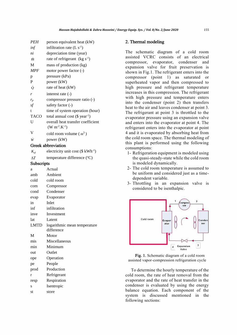
2. Thermal modeling The schematic diagram of a cold room assisted VCRC consists of an electrical compressor, evaporator, condenser and expansion valve for fruit preservation is shown in Fig.1. The refrigerant enters into the compressor (point 1) as saturated or superheated vapor and then compressed to high pressure and refrigerant temperature increases in this compression. The refrigerant with high pressure and temperature enters into the condenser (point 2) then transfers heat to the air and leaves condenser at point 3. The refrigerant at point 3 is throttled to the evaporator pressure using an expansion valve and enters into the evaporator at point 4. The refrigerant enters into the evaporator at point 4 and it is evaporated by absorbing heat from the cold room space. The thermal modeling of this plant is performed using the following consumptions: 1- Refrigeration equipment is modeled using
the quasi-steady-state while the cold room is modeled dynamically.
2- The cold room temperature is assumed to be uniform and considered just as a time-dependent variable.
3- Throttling in an expansion valve is considered to be isenthalpic.
Fig. 1. Schematic diagram of a cold room
assisted vapor-compression refrigeration cycle
To determine the hourly temperature of the cold room, the rate of heat removal from the evaporator and the rate of heat transfer in the condenser is evaluated by using the energy balance equation. Each component of the system is discussed mentioned in the following sections:
156 Hassan Hajabdollahi & Zahra Hosseini / Energy Equip. Sys. / Vol. 8/No. 2/June 2020
2.1. Compressor
The isentropic efficiency of the compressor is determined as [23]:
, 1 2
1 2,
com s scom
acom a
W h h
h hW
,
(1)
where h indicates the enthalpy in each point. Moreover, subscript s and a are the isentropic and actual states of the compressor, respectively. On the other hand, the compressor isentropic efficiency can be defined in terms of pressure ratio as [24]:
1 2 ( )com pc c r (2)
where rp is the compressor pressure ratio
2 1( / )p p.
2.2. Heat exchangers (condenser and
evaporator) The first law of thermodynamic for the condenser and evaporator leads to
2 3( )r LMTDQ m h h FUA T , (3)
in which rm is the mass flow rate of
refrigerant and U , A, F and LMTDT are, respectively, the overall heat transfer coefficient, condenser (or evaporator) heat transfer surface area, flow arrangement correction factor and logarithmic mean temperature difference which is defined as
2 , 3 ,1 2
,1 2 2 , 3 ,
log( / ) log /
air out air in
LMTD cond
air out air in
T T T TT TT
T T T T T T
,
(4) for the condenser, and
, 1 , 4
,
, 1 , 4log /
cold in cold out
LMTD evap
cold in cold out
T T T TT
T T T T
,
(5)
for the evaporator.
2.3. Expansion valve The refrigerant is throttled from the condenser and then entered into the evaporator by passing into the expansion valve with constant enthalpy (h3=h4).
2.4. Cold room
Due to the variation of some parameters such as ambient temperature and evaporator heat removal by time (on or off), the cold room temperature is also a function of time and should be determined. For this purpose, using the energy conservation law for the entire cold room system as a control volume we have:
in out stE E E , (6)
( ( 1) ( )) /loss cycle pQ Q Mc T t T t dt
and
(7)
( 1) (( ) / ) ( )loss cycle pT t Q Q dt Mc T t . (8)
Here the constant values of MCP is the sum of total heat capacity and mass of both air and production in the cold room. In addition, T (t+1) is the hourly temperature of the cold
room and cycleQ is the capacity of system
cooling. In fact, cycle evapQ Q in the case of
running an evaporator while it is 0cycleQ
in the case of turning off the evaporator. It should be mentioned that the strategy of evaporator running on or off should be determined based on cold room temperature which is discussed in the next sections.
Moreover, lossQin the above relation is the
heat loss from the cold room is obtained by
inf( )loss wall prod resp mis latQ Q Q Q Q Q Q sf (9)
where sf is a safety factor. The heat loss consists of the load from wall’s cold room, production load, respiration heat, miscellaneous load, latent load and the infiltration load, which is estimated as
wall wall wallQ U A T , (10)
( / (24 3600 ))prod p prodQ M c T cf , (11)
( ) /1000resp respQ M q , (12)
(( ) / 24 ( ) / 24 ( ) / 24)mis bulb pe MQ P t n PEH t P MPF t (13)
( ) / 24 3600lan lanQ M q and (14)
0.449inf infQ V dh . (15)

Hassan Hajabdollahi & Zahra Hosseini / Energy Equip. Sys. / Vol. 8/No. 2/June 2020 157
Here U, A and T are, respectively, the overall heat transfer coefficient, required heat transfer surface area for cold room and difference temperature between the inside and
outside of the cold room. In addition, M, lanq
, cp, Cf, p, PEH and MPF are total production mass, latent load in the cold room, specific heat factor, chilling factor, bulb power, person equivalent heat and motor power factor, respectively. Moreover, n, t, inf, V and dh are the number of people in the cold room, system operating time, infiltration rate, cold room volume and change of enthalpy.
Finally, the coefficient of performance (COP) of the system is defined as the ratio of the desired output to the required input as
Ni
i
icom
Ni
i
ievap
W
Q
COP
1
,
1
,
,
(16)
where N is the operating hours of the system in a year. 3. Economic Modeling In this paper, two important parameters are considered as objective functions and optimized simultaneously. The first one is the COP, which is defined in equation (16). The second one is the total annual cost (TACO), including the capital cost of VCRC components and cold room as well as the operating cost of compressor, estimated as
total inve opeC aC C , (17)
3 51 2 4
, , , , ,
1 2 3 4 5( ) ( ) ( ) ( ) ( )
inve inve cond inve evap inve com inve ev inve cold
m mm m mcond evap com r cold
C C C C C C
n A n A n W n m n V
(18)
,ope ope com com ope elC C W H K , (19)
where the values of n and m are constant and evaluated using the regional price. In
addition, Hope and Kel are yearly operational hours and the electricity unit cost, respectively. Moreover, a is the annualized factor in terms of interest rate (r) and system lifetime (ni) given as [28]
1 (1 ) ni
ra
r
.
(20)
4. Objective functions, decision variables and constraints
In this paper, the COP and TACO are considered as objective functions and evaporator pressure, condenser pressure, cold room length, cold room wall thickness, cold room height, the mass flow rate of refrigerant along with the value of evaporator superheating and condenser subcooling are selected as decision variables. Moreover, the following constraint is also considered in the optimization process:
1.1pr . (21)
The following relation is considered to keep the condenser temperature above that of the ambient for having the heat transfer:
2 ,max 10ambT T . (22)
Furthermore, the following constraint is also considered to have a reasonable temperature difference between the evaporator and cold room temperature:
4 5T . (23)
Finally, for keeping the quality of the production, the maximum and minimum temperature of the cold room should be in the range of 0.5-1.5 oC as:
max, 1.5coldT and (24)
min, 0.5coldT . (25)
5. Solution Trend The procedure of modeling and optimization of the cold room is depicted in Fig. 2 and summarized as follow:
1- MOGA parameters such as the number of chromosomes, mutation probability, controlled elitism value, crossover probability are adjusted.
2- The initial population is generated, and the number of bit for each variable is obtained.
3- Thermodynamic properties of refrigerants are calculated for each chromosome by using the EES database.
4- Thermo-economic modeling is performed for each chromosome using nine design parameters.

158 Hassan Hajabdollahi & Zahra Hosseini / Energy Equip. Sys. / Vol. 8/No. 2/June 2020
5- The following procedure is performed in each hour of a year, and then the objective functions are determined.
6- This process is repeated from stage 3 until the convergence.
Fig.2. Flowchart of modeling and optimization
6. Case study A cold room assisted vapor-compression refrigeration cycle is thermodynamically modelled then optimized. The optimization process is used for a cold room located in Rafsanjan city, one of the cities in the Kerman province of Iran. This cold room should be designed for keeping 500 tons of apple. Furthermore, two persons with a 4.17 kW lift
truck work in the cold room for 3 hours each day. Besides, the safety factor, chilling rate factor, and design dry temperature of the air in winter are considered 1.1, 1 and -3.2, respectively [25]. If the temperature of cold room space is higher than 1.1, the evaporator is on, and it is evaporated by capturing heat from the cold room space else if the temperature of cold room space is lower than 0.9 the evaporator is off. In addition the constants of investment cost used in equation (18) are taken n= (748.6, 499.1, 233.3, 400, 295) and m= (0.16, 0.16, 0.95, 1, 1) based on market available price [1].
7. Results and discussion
7.1. Optimization results Five refrigerants included R22, R134a, R407c, R245 and R123 are chosen, and the plant is optimized for each case separately. Design parameters, along with the range of their variations, are shown in Table 1.
The Genetic Algorithm is iterated for 4000 generations, using chromosome number of
n=100 mutation probability of Pm=0.045, elitism parameter of c=0.55, and crossover
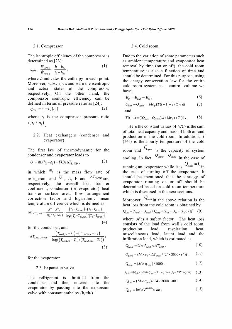
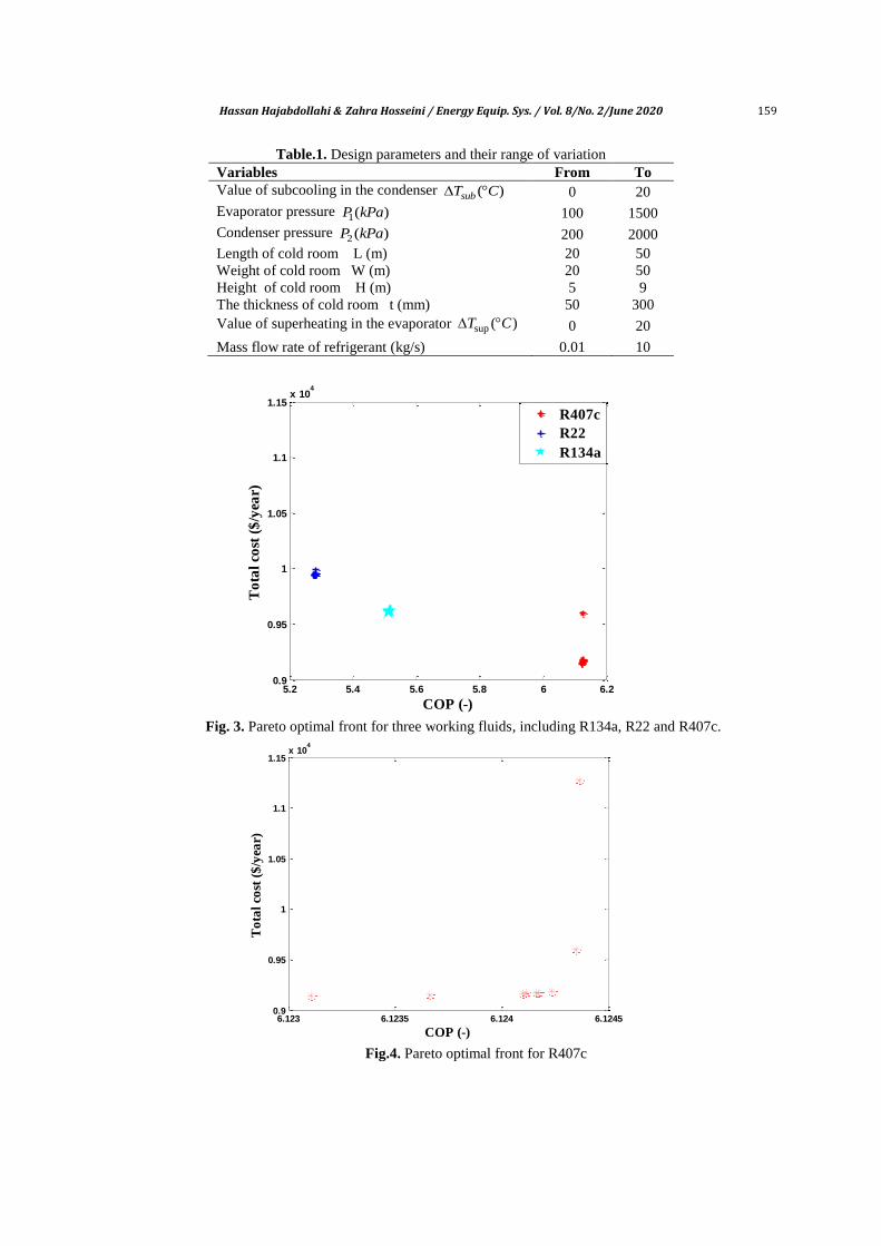
probability of pc=0.9, separately for five refrigerants including R134a, R407c, R245fa, R123 bbbb and R22. It is worth noting that, due to the constraints introduced in section 4, there are no optimum results for a system working with R245fa and R123. The results of optimum COP and total annual cost (TACO) for three remain refrigerants are shown in Fig. 3. The optimum Pareto fronts reveal that, unlike some thermal systems such as heat exchangers and power generation systems [27-30], we have a point with simultaneous optimum cost and COP. In fact, in the maximum point of COP, the minimum point of TACO is observed. Moreover, it is observed that the best-studied working fluid is R407c and respectively, followed by R22 and R134a. The Pareto optimal front for the best-studied working fluid (R407c) is also separately shown in Fig. 4. It is observed that the maximum COP is 6.12, while the minimum TACO is 9148.2 $/year.
Hassan Hajabdollahi & Zahra Hosseini / Energy Equip. Sys. / Vol. 8/No. 2/June 2020 159
Table.1. Design parameters and their range of variation
Variables From To
Value of subcooling in the condenser ( )subT C 0 20
Evaporator pressure 1( )P kPa 100 1500
Condenser pressure 2( )P kPa 200 2000
Length of cold room L (m) 20 50
Weight of cold room W (m) 20 50
Height of cold room H (m) 5 9
The thickness of cold room t (mm) 50 300
Value of superheating in the evaporator sup ( )T C 0 20
Mass flow rate of refrigerant (kg/s) 0.01 10
Fig. 3. Pareto optimal front for three working fluids, including R134a, R22 and R407c.
Fig.4. Pareto optimal front for R407c
5.2 5.4 5.6 5.8 6 6.20.9
0.95
1
1.05
1.1
1.15x 10
4
COP (-)
To
tal
cost
($
/yea
r)
R407c
R22
R134a
6.123 6.1235 6.124 6.12450.9
0.95
1
1.05
1.1
1.15x 10
4
COP (-)
To
tal
cost
($
/yea
r)
160 Hassan Hajabdollahi & Zahra Hosseini / Energy Equip. Sys. / Vol. 8/No. 2/June 2020
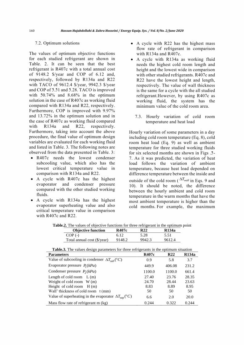
7.2. Optimum solutions The values of optimum objective functions for each studied refrigerant are shown in Table. 2. It can be seen that the best refrigerant is R407c with a total annual cost of 9148.2 $/year and COP of 6.12 and, respectively, followed by R134a and R22 with TACO of 9612.4 $/year, 9942.3 $/year and COP of 5.51 and 5.28. TACO is improved with 50.74% and 8.68% in the optimum solution in the case of R407c as working fluid compared with R134a and R22, respectively. Furthermore, COP is improved with 9.97% and 13.72% in the optimum solution and in the case of R407c as working fluid compared with R134a and R22, respectively. Furthermore, taking into account the above procedure, the final value of optimum design variables are evaluated for each working fluid and listed in Table. 3. The following notes are observed from the data presented in Table. 3: R407c needs the lowest condenser
subcooling value, which also has the lowest critical temperature value in comparison with R134a and R22.
A cycle with R407c has the highest evaporator and condenser pressure compared with the other studied working fluids.
A cycle with R134a has the highest evaporator superheating value and also critical temperature value in comparison with R407c and R22.
A cycle with R22 has the highest mass flow rate of refrigerant in comparison with R134a and R407c.
A cycle with R134a as working fluid needs the highest cold room length and height and the lowest wide in comparison with other studied refrigerants. R407c and R22 have the lowest height and length, respectively. The value of wall thickness is the same for a cycle with the all studied refrigerant.However, by using R407c as working fluid, the system has the minimum value of the cold room area.
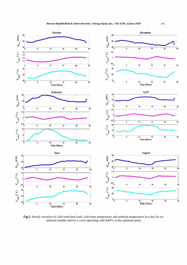
7.3. Hourly variation of cold room temperature and heat load
Hourly variation of some parameters in a day including cold room temperature (Eq. 8), cold room heat load (Eq. 9) as well as ambient temperature for three studied working fluids for six selected months are shown in Figs .5-7. As it was predicted, the variation of heat load follows the variation of ambient temperature, because heat load depended on difference temperature between the inside and
outside of the cold room ( wallT in Eqs. 9 and 10). It should be noted, the difference between the hourly ambient and cold room temperature in the warm months that have the most ambient temperature is higher than the cold months. For example, the maximum
Table.2. The values of objective functions for three refrigerant in the optimum point
Objective function R407c R22 R134a
COP (-) 6.12 5.28 5.51
Total annual cost ($/year) 9148.2 9942.3 9612.4
Table.3. The values design parameters for three refrigerants in the optimum situation
Parameters R407c R22 R134a
Value of subcooling in condenser ( )subT C 0.9 5.8 3.7
Evaporator pressure 1( )P kPa 449.9 406.08 231.2
Condenser pressure 2( )P kPa 1100.0 1100.0 661.4
Length of cold room L (m) 27.40 23.76 28.35
Weight of cold room W (m) 24.70 28.44 23.63
Height of cold room H (m) 8.83 8.89 8.95
Wall’ thickness of cold room t (mm) 50 50 50
Value of superheating in the evaporator sup ( )T C 6.6 2.0 20.0
Mass flow rate of refrigerant m (kg) 0.244 0.322 0.244
Hassan Hajabdollahi & Zahra Hosseini / Energy Equip. Sys. / Vol. 8/No. 2/June 2020 161
Fig.5. Hourly variation of cold room heat load, cold room temperature and ambient temperature in a day for six
selected months and for a cycle operating with R407c in the optimum point
162 Hassan Hajabdollahi & Zahra Hosseini / Energy Equip. Sys. / Vol. 8/No. 2/June 2020
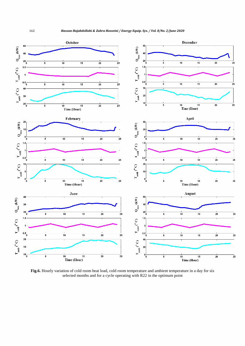
Fig.6. Hourly variation of cold room heat load, cold room temperature and ambient temperature in a day for six
selected months and for a cycle operating with R22 in the optimum point

Hassan Hajabdollahi & Zahra Hosseini / Energy Equip. Sys. / Vol. 8/No. 2/June 2020 163
Fig.7. Hourly variation of cold room heat load, cold room temperature and ambient temperature in a day for six
selected months and for a cycle operating with R134a in the optimum point

164 Hassan Hajabdollahi & Zahra Hosseini / Energy Equip. Sys. / Vol. 8/No. 2/June 2020
differences in February are 9.11, 9.12, and 9.11 oC respectively for R407c, R22 and R134a. The mentioned values are 29.50, 29.52, and 29.52 oC in August.
As was mentioned, the evaporator is running in the situation in which the cold room temperature is higher than 1.1 while it is off in the situation in which the cold room temperature is lower than 0.9. It is clear that in the warmer months (August) in Figs .5-7, the number strategy of evaporator running on, is increased and in coldest months (February) in Figs .5-7 is vice versa. From these figures, the variation of hourly temperature and hourly heat load of cold room for R407c and R134a has a small difference because the
optimum values of lossQ and coldT are in the same range with a small difference. The average of the mentioned parameters for each working fluids in six months of the year is listed in Tables.4-6. The following points from the results listed in Tables.4-6 could be deduced: 1. In the warmest (August) and coldest
(February) month, R22 has the highest heat load average. R407c and R134a are in in the next ranking, respectively.
2. Also, in the coldest month (February), R134a has the lowest average heat load. R407c and R22 are in in the next ranking, respectively.
3. The maximum value of cold room`s hourly average temperature in the warmest month (August) that occurred by using R407c as working fluids, is more than this value in the coldest month (February).
4. The average ambient average temperature in a day of the coldest month (February) is 4.40 C, whereas, in this time, the cold room has a minimum value of hourly average temperature with 0.99 centigrade by using R407c and R22as working fluids. Also, the maximum of this value is 1.01 centigrade by using R134a as working fluids.
5. The average of ambient average temperature in a day of the warmest month (August) is 24.29 centigrade, whereas, in this time, the cold room has a maximum value of hourly average temperature by using R407c, R134a and R22, respectively.
Table.4. The average values of hourly temperature of the cold room, the hourly temperature of Rafsanjan city
and hourly heat load of the cold room in six selected months for R407c
October December February April June August
lossQ 46.76 33.71 12.73 22.90 27.22 37.65
coldT 1.34 1.00 0.99 0.99 1.00 1.05
ambT 31.17 21.27 4.40 12.55 15.97 24.29
Table.5. The average values of hourly temperature of the cold room, the hourly temperature of Rafsanjan city
and hourly heat load of the cold room in six selected months for R22
October December February April June August
lossQ 47.17 33.73 12.74 22.90 27.25 37.74
coldT 1.04 1.00 0.99 1.00 1.00 1.00
ambT 31.17 21.27 4.40 12.55 15.97 24.29
Table.6. The average values of hourly temperature of the cold room, the hourly temperature of Rafsanjan city
and hourly heat load of the cold room in six selected months for R134a
October December February April June August
lossQ 46.67 33.63 12.71 22.85 27.19 37.64
coldT 1.36 1.02 1.01 1.01 1.00 1.01
ambT 31.17 21.27 4.40 12.55 15.97 24.29

Hassan Hajabdollahi & Zahra Hosseini / Energy Equip. Sys. / Vol. 8/No. 2/June 2020 165
8. Conclusions A cold room assisted the vapor-compression refrigeration cycle was designed and optimized usingthe genetic algorithm. Evaporator pressure, condenser pressure, the mass flow rate of refrigerant, the value of evaporator superheating, the value of condenser subcooling along with the physical specification of the cold room were selected as decision variables. In the studied optimization problem, TACO and COP were selected as fitness functions. The optimization was done for three refrigerants, including R134a, R407C and R22. The optimization results show that a cycle operating with R407c leads to the best results compared with the other studied refrigerants. For example, 50.74%, and 8.68% improvements in the total annual cost were found in the case of R407c as working fluid compared with R134a and R22, respectively. The above improvements were 9.97% and 13.72% for COP. It is worth mentioning that the optimum results reveal that, unlike some thermal systems such as heat exchanger and power plants, there is no conflicting behavior between the selected thermo-economic objective functions, and a cycle with the highest COP has the lowest annual cost. Furthermore, a cycle operating with R407c needs the lowest cold room height while a cycle with R22 needs the lowest cold room length. The value of cold room wall thickness is the same for all studied refrigerants. Also, by using R407c as the working refrigerant, the cold room needs the minimum area. References [1] Çengel, Y. A. and Boles, M. A., 2006.
Thermodynamics: An Engineering Approach, McGraw-Hill.
[2] Zhu, L. and Yu, J., 2015. Theoretical study of a thermoelectric-assisted vapor compression cycle for air-source heat pump applications. International Journal of Refrigeration, 51, pp.33-40.
[3] Xu, Y.C. and Chen, Q., 2013. A theoretical global optimization method for vapor-compression refrigeration
systems based on entransy theory. Energy, 60, pp.464-473.
[4] Yan, G., Cui, C. and Yu, J., 2015. Energy and exergy analysis of zeotropic mixture R290/R600a vapor-compression refrigeration cycle with separation condensation. International Journal of Refrigeration, 53, pp.155-162.
[5] Molés, F., Navarro-Esbrí, J., Peris, B., Mota-Babiloni, A. and Barragán-Cervera, Á. 2014. Theoretical energy performance evaluation of different single-stage vapor compression refrigeration configurations using R1234yf and R1234ze (E) as working fluids. International Journal of Refrigeration, 44, pp.141-150.
[6] Nunes, T.K., Vargas, J.V.C., Ordonez, J.C., Shah, D. and Martinho, L.C.S., 2015. Modeling, simulation and optimization of a vapor compression refrigeration system dynamic and steady-state response. Applied Energy, 158, pp.540-555.
[7] Brito, Paulo, Pedro Lopes, Paula Reis, and Octávio Alves. "Simulation and optimization of energy consumption in cold storage chambers from the horticultural industry." International Journal of Energy and Environmental Engineering 5, no. 2-3 (2014): 1-15.
[8] Domanski, P.A., Brown, J.S., Heo, J., Wojtusiak, J. and McLinden, M.O., 2014. A thermodynamic analysis of refrigerants: Performance limits of the vapor compression cycle. International Journal of Refrigeration, 38, pp.71-79.
[9] Jain, V., Kachhwaha, S.S. and Sachdeva, G., 2013. Thermodynamic performance analysis of a vapor compression–absorption cascaded refrigeration system. Energy Conversion and Management, 75, pp.685-700.
[10] Jain, V., Sachdeva, G. and Kachhwaha, S.S., 2015. Thermodynamic modeling and parametric study of a low-temperature vapor compression-absorption system based on modified Gouy-Stodola equation. Energy, 79, pp.407-418.
[11] Jensen, Jonas K., Wiebke B. Markussen, Lars Reinholdt, and Brian Elmegaard. "Exergoeconomic
166 Hassan Hajabdollahi & Zahra Hosseini / Energy Equip. Sys. / Vol. 8/No. 2/June 2020
optimization of an ammonia–water hybrid absorption–compression heat pump for heat supply in a spray-drying facility." International Journal of Energy and Environmental Engineering 6, no. 2 (2015): 195-211.
[12] Yataganbaba, A., Kilicarslan, A. and Kurtbaş, İ., 2015. Exergy analysis of R1234yf and R1234ze as R134a replacements in a two evaporator vapor compression refrigeration system. International Journal of Refrigeration, 60, pp.26-37.
[13] Arora, A. and Kaushik, S.C., 2008. Theoretical analysis of a vapour compression refrigeration system with R502, R404A and R507A.International journal of refrigeration, 31(6), pp.998-1005.
[14] Yang, M.H. and Yeh, R.H., 2015. Performance and exergy destruction analyses of optimal subcooling for vapor-compression refrigeration systems. International Journal of Heat and Mass Transfer, 87, pp.1-10.
[15] Jain, N. and Alleyne, A., 2015. Exergy-based optimal control of a vapor compression system. Energy Conversion and Management, 92, pp.353-365.
[16] Nikolaidis, C. and Probert, D., 1998. Exergy-method analysis of a two-stage vapour-compression refrigeration-plants performance. Applied Energy, 60(4), pp.241-256.
[17] Jain, V., Sachdeva, G. and Kachhwaha, S.S., 2015. Energy, exergy, economic and environmental (4E) analyses based comparative performance study and optimization of vapor compression-absorption integrated refrigeration system—energy, 91, pp.816-832.
[18] Torrella, E., Larumbe, J.A., Cabello, R., Llopis, R. and Sanchez, D., 2011. A general methodology for energy comparison of intermediate configurations in two-stage vapour compression refrigeration systems. Energy, 36(7), pp.4119-4124.
[19] Hoang, H.M., Duret, S., Flick, D. and Laguerre, O., 2015. Preliminary study of airflow and heat transfer in a cold room
filled with apple pallets: Comparison between two modelling approaches and experimental results. Applied Thermal Engineering, 76, pp.367-381.
[20] Laguerre, O., Duret, S., Hoang, H.M., Guillier, L. and Flick, D., 2015. Simplified heat transfer modeling in a cold room filled with food products. Journal of Food Engineering, 149, pp.78-86.
[21] Khademi, Maryam, Atefeh Behzadi Forough, and Ahmad Khosravi. "Techno-economic operation optimization of a HRSG in combined cycle power plants based on evolutionary algorithms: A case study of Yazd, Iran." Energy Equipment and Systems 7, no. 1 (2019): 67-79.
[22] Hajabdollahi, Hassan, and Alireza Esmaieli. "Selection of the optimum prime mover and the working fluid in a regenerative organic Rankine cycle." Energy Equipment and Systems 5, no. 4 (2017): 325-339.
[23] Khorasaninejad, E. and Hajabdollahi, H., 2014. Thermo-economic and environmental optimization of the solar-assisted heat pump by using a multi-objective particle swarm algorithm. Energy, 72, pp.680-690.
[24] Sayyaadi, H., Amlashi, E.H. and Amidpour, M., 2009. Multi-objective optimization of a vertical ground source heat pump using an evolutionary algorithm. Energy Conversion and Management, 50(8), pp.2035-2046.
[25] Dossat, Roy. j., 2009. Principles of Refrigeration.
[26] Hajabdollahi, H., Ganjehkaviri, A. and Jaafar, M.N.M., 2015. Assessment of new operational strategy in the optimization of CCHP plant for different climates using evolutionary algorithms. Applied Thermal Engineering, 75, pp.468-480.
[27] Hajabdollahi, Z., Hajabdollahi, F., Tehrani, M. and Hajabdollahi, H., 2013. Thermo-economic environmental optimization of Organic Rankine Cycle for diesel waste heat recovery. Energy, 63, pp.142-151.
[28] Hajabdollahi, H., 2015. Investigating the effect of non-similar fins in

Hassan Hajabdollahi & Zahra Hosseini / Energy Equip. Sys. / Vol. 8/No. 2/June 2020 167
thermoeconomic optimization of plate fin heat exchanger. Applied Thermal Engineering, 82, pp.152-161.
[29] Hajabdollahi, H., Ahmadi, P. and Dincer, I., 2011. Multi-objective optimization of plain fin-and-tube heat exchanger using an evolutionary algorithm. Journal of thermophysics and heat transfer, 25(3), pp.424-431.
[30] Hajabdollahi, H., Hosseinni, Z., 2016. Multi-objective optimization of steam cycle power plant using NSGA-II, 24th International Conference in mechanical engineering (ISME), Yazd, Iran.