modelling tropospheric gradients and parameters from nwp models… · 2011-11-15 · technical...

MODELLING TROPOSPHERIC GRADIENTS AND PARAMETERS FROM NWP MODELS: EFFECTS

ON GPS ESTIMATES

REZA GHODDOUSI-FARD

February 2009

TECHNICAL REPORT NO. 264

MODELLING TROPOSPHERIC GRADIENTS AND PARAMETERS FROM NWP MODELS:

EFFECTS ON GPS ESTIMATES

Reza Ghoddousi-Fard

Department of Geodesy and Geomatics Engineering University of New Brunswick

P.O. Box 4400 Fredericton, N.B.

Canada E3B 5A3

February 2009

© Reza Ghoddousi-Fard 2009

PREFACE

This technical report is a reproduction of a dissertation submitted in partial fulfillment

of the requirements for the degree of Doctor of Philosophy in the Department of Geodesy

and Geomatics Engineering, February 2009. The research was supervised by Dr. Peter

Dare, and funding was provided by the Natural Sciences and Engineering Research

Council of Canada, the Canada Foundation for Innovation, the New Brunswick

Innovation Foundation, Northern Scientific Training Program of Indian and Northern

Affairs Canada, and the Royal Institution of Chartered Surveyors Education Trust.

As with any copyrighted material, permission to reprint or quote extensively from this

report must be received from the author. The citation to this work should appear as

follows:

Ghoddousi-Fard, Reza (2009). Modelling Tropospheric Gradients and Parameters from

NWP Models: Effects on GPS Estimates. Ph.D. dissertation, Department of Geodesy and Geomatics Engineering, Technical Report No. 264, University of New Brunswick, Fredericton, New Brunswick, Canada, 216 pp.

ii

ABSTRACT

The neutral atmosphere delay still remains one of the most limiting accuracy factors in

global navigation satellite systems (GNSS) and other radiometric space-geodesy

techniques. Due to the fact that the neutral atmosphere is a non-dispersive medium, the

use of dual frequency approaches cannot eliminate the effect of neutral atmosphere delay

at radio frequencies.

In recent years the use of numerical weather prediction (NWP) models has been

investigated to mitigate the neutral atmosphere delay on GNSS signals. However, due to

the practical issues NWP-based approaches have not yet been widely used by GNSS

users. A spherically symmetric atmosphere has been a common assumption in GNSS

processing for a long time. As NWP models provide the 3-D state of the neutral

atmosphere, the motivation has been raised to consider the asymmetry of the neutral

atmosphere in GNSS processing.

In this dissertation recent developments in NWP-based modeling of neutral atmosphere

delay are reviewed and compared. As an example of an NWP-for-GNSS operational

service an online ray tracing package has been developed which has been accessible to

the public for the past 2 years. Routine 3-hourly global maps of zenith delay, gradients

and comparison with climate-based models have been also generated.

iii

Asymmetry of the hydrostatic part of the neutral atmosphere has been modeled based on

a dual radiosonde ray tracing approach developed for part of North America. An

approach based on a semi-3-D retrieval of delays from NWP models also has been

developed. The NWP-based parameters including zenith delays, mapping functions and

gradients have been implemented in the Bernese GPS software. This made the software

capable of correcting pseudorange observables in all related processing options.

Modified software has been employed to study the effect of the implemented NWP-based

processing on GPS estimated parameters. The result of a month-long precise point

positioning experiment shows millimetre-level improvement in the latitude component at

most of the stations when hydrostatic gradients are introduced as a priori. Height and

zenith tropospheric delay parameters are also affected by implementing NWP-based

gradients as well as by implementing zenith delay values and mapping functions even

though the effects were not found to be systematic.

Based on the results of this dissertation research, implementing NWP-based parameters

in GPS processing for high accuracy applications such as geodynamics, realization of

terrestrial reference frames, and climatology are suggested. This is now possible with the

modified Bernese software which is capable of considering NWP hydrostatic, non-

hydrostatic and total gradients as a priori in GPS observables as well as zenith delay and

mapping functions based on NWP models in all processing strategies.

iv

ACKNOWLEDGEMENTS

I would like to thank my supervisor Dr. Peter Dare for his support, patience and

opportunities throughout my PhD studies. I would also like to thank Dr. Richard Langley

for his comments during weekly GPS group meetings. Thanks also go to Dr. Don Kim

and other members of the examination committee: Dr. William Ward from UNB’s

Department of Physics and Dr. Johannes Boehm from Institute of Geodesy and

Geophysics at the Vienna University of Technology, Austria.

The financial support from Canada’s Natural Sciences and Engineering Research

Council, Canada Foundation for Innovation, the New Brunswick Innovation Foundation,

Northern Scientific Training Program of Indian and Northern Affairs Canada, and the

Royal Institution of Chartered Surveyors Education Trust are acknowledged.

The Chair and staff at UNB’s Ocean Mapping Group are thanked for providing support

during my data collection exercise onboard the Canadian research icebreaker Amundsen

during her 2005 Canadian Arctic and Hudson Bay expedition. Environment Canada’s

Meteorological Service of Canada, and its Canadian Meteorological Centre, the U.S.

National Oceanic and Atmospheric Administration, and the International GNSS Service

are thanked for providing data access. I also thank the Atlantic Computational Excellence

Network for providing computing resources.

v

Thanks also go to office staff of the Department of Geodesy and Geomatics Engineering

and UNB’s Integrated Technology Services for their support. I would like to express my

thanks to all fellow graduate students in the Geodetic Research Laboratory for their

friendship.

Finally, I wish to thank my parents for their endless support during my life. This work is

dedicated to them.

vi

Table of Contents

ABSTRACT........................................................................................................................ ii

ACKNOWLEDGEMENTS............................................................................................... iv

Table of Contents............................................................................................................... vi

List of Tables ...................................................................................................................... x

List of Figures ................................................................................................................... xii

List of Abbreviations ..................................................................................................... xxiii

Chapter 1: Introduction ....................................................................................................... 1 1.1- Background and Motivation .................................................................................... 1

1.2- Dissertation Contribution ........................................................................................ 8

1.3- Dissertation outline................................................................................................ 10

Chapter 2: Effect of the Neutral Atmosphere on GNSS Signals ..................................... 12 2.1- The Neutral Atmosphere ....................................................................................... 12

2.2- Neutral Atmospheric Delay in GNSS Observables ............................................... 18

2.3- Neutral Atmospheric Models and Mapping Functions.......................................... 21

2.3.1- Zenith Hydrostatic (and Dry) Delay Models.................................................. 22

2.3.2- Zenith Non-Hydrostatic (and Wet) Delay Models ......................................... 22

2.3.3- Mapping Functions ......................................................................................... 23

2.3.4- Modeling the Meteorological Parameters....................................................... 24

2.4- Summary................................................................................................................ 25

Chapter 3: Recent Developments in Neutral Atmosphere Mapping Functions................ 27 3.1- Recent Symmetric Mapping Functions ................................................................. 27

3.1.1- Niell Mapping Functions ................................................................................ 27

3.1.2- Isobaric Mapping Functions ........................................................................... 31

vii

3.1.3- Vienna Mapping Functions ............................................................................ 33

3.1.4- Global Mapping Functions ............................................................................. 36

3.1.5- Comparison of Recent Symmetric Mapping Functions ................................. 38

3.2- Gradient Models and Mapping Functions ............................................................. 45

3.2.1- Davis et al. ...................................................................................................... 46

3.2.2- Chen and Herring............................................................................................ 47

3.2.3- Tilting of the Atmosphere............................................................................... 48

3.2.4- Niell Hydrostatic Gradient Mapping Function............................................... 51

3.3- Summary................................................................................................................ 53

Chapter 4: Ray Tracing: Theory and Practice................................................................... 54 4.1- Ray Tracing: A Review ......................................................................................... 54

4.1.1- Delay Integration ............................................................................................ 66

4.2- Data Sources for Ray Tracing ............................................................................... 69

4.2.1- Radiosonde ..................................................................................................... 70

4.2.1.1- Radiosonde Uncertainty Effects on Zenith Delay …………………….71

4.2.2- NWP Models .................................................................................................. 75

4.3-Online Ray Tracing Package .................................................................................. 77

4.4- Validation of Results ............................................................................................. 85

4.4.1- Water Vapour Radiometer.............................................................................. 85

4.4.2- Precise Barometer and WVR on a Moving Platform for NWP Validation.... 87

4.4.3- Validation at RAOB Locations and WVR at UNB ........................................ 95

4.4.4- Summary of Validation Results.................................................................... 100

viii

Chapter 5: Modelling and Estimation of Neutral Atmospheric Delay Gradients........... 101 5.1- Modelling Regional Hydrostatic Gradients Using a Dual Radiosonde Ray Tracing

Approach..................................................................................................................... 101

5.1.1- A Regional Study.......................................................................................... 104

5.1.2- Modelling Azimuth-dependent Hydrostatic Slant Delays............................ 109

5.2- Estimation of Horizontal Delay Gradients from NWP Models........................... 113

5.3- Comparison of Different Gradient Retrieval Approaches ................................... 117

5.3.1- Comparison of NWP-retrieved Gradients from Two Different Models and

Algorithms .............................................................................................................. 120

5.4- Studying Temporal Variations of Gradients........................................................ 122

5.5- GPS-estimated Gradients..................................................................................... 131

5.5.1- Gradient Estimation Interval Effect.............................................................. 136

5.6- Summary.............................................................................................................. 138

Chapter 6: NWP-based Parameters in GPS Software: Analysis and Results ................. 139 6.1- A Semi-3-D NWP-Based Neutral Atmospheric Correction................................ 139

6.2- Software Implementation .................................................................................... 143

6.2.1- Clock Synchronization and Code Zero-Difference Solution........................ 146

6.2.2- Pre-Processing of Phase Observations ......................................................... 152

6.2.3- Main Parameter Estimation .......................................................................... 154

6.2.4- Combination of Solutions............................................................................. 155

6.3- Effect of NWP-Based Corrected Pseudo-ranges on PPP Estimates.................... 155

6.3.1- Data Analysis and Results ............................................................................ 158

6.3.1.1- Effect of NMP-based ZHD and Mapping Function …………………162

ix

6.3.1.2- Effect of NWP-based A Priori Hydrostatic Gradients ………………164

6.3.2- Discussion..................................................................................................... 177

Chapter 7: Conclusions and Recommendations ............................................................. 179

References....................................................................................................................... 184

Appendix I: List of Radiosonde Stations Used in Dual Ray Tracing and Validation Studies............................................................................................................................. 193

Appendix II: Monthly Plots of Differences between Dual and Single RAOB Ray Tracing and a Fitted Function ...................................................................................................... 196

Appendix III: Sample Online-RT Maps ......................................................................... 203

Appendix IV: Bernese Modification Flow Diagrams..................................................... 211

Appendix V: NWP Input File Format Defined for Modified Bernese ........................... 215

Curriculum Vitae

x

List of Tables

Table 3.1- Coefficients for NMF ...................................................................................... 29

Table 3.2- Parameters in equation (3.11) for hydrostatic VMF1...................................... 35

Table 3.3- Parameters in equation (3.11) for total VMF1 ................................................ 35

Table 4.1- Accuracy of related radiosonde measurements that shall be considered as

minimum standard [FMH, 1997]. ..................................................................................... 74

Table 4.2- Difference between global and regional NWP model results ......................... 96

Table 4.3- Statistics of comparison results between NWP models and RAOB................ 97

Table 4.4- Difference between measurement (barometer and Saastamoinen model for

ZHD and WVR for ZWD) and NWP models. ................................................................ 100

Table 5.1- Estimated parameters of exponential fit to NS (index N) and EW (index E)

components together with RMS of the fits. Unit: metre. ................................................ 112

Table 5.2- Statistics of temporal variation of gradients and zenith delays (mm/3 hours)

calculated over the month of July 2007. Pr(0.95) is the max absolute change (mm/3

hours) in 95% probability. .............................................................................................. 126

Table 5.3- Statistics of temporal variation of gradients and zenith delays (mm/3 hours)

calculated over the month of January 2008. Pr(0.95) is the max absolute change (mm/3

hours) at 95% probability................................................................................................ 129

Table 5.4– Statistics of difference between PPP estimation results under various gradient

estimation intervals and IGS solution. Station: ALGO, July, 2007. N/A indicates relative

constraining is not applied. ............................................................................................. 137

xi

Table 6.1- Approximate position, receiver and antenna type of the investigated stations.

......................................................................................................................................... 162

Table 6.2- Extreme differences between results of scenarios 1 and 2. ........................... 163

Table 6.3- RMS and max. abs. diff. between ZHD from NWP and Saastamoinen

calculated over month of July 2007 at the investigated stations..................................... 164

Table 6.4- Statistics of the comparisons between scenarios 2 and 3. ............................. 173

Table 6.5- Statistics of scenario 1 results vs. IGS values. .............................................. 174



Table I.1– Location and code of radiosondes ................................................................. 193

xii

List of Figures

Figure 2.1- The Earth’s atmospheric layers and the neutral atmosphere (after Langley

[1998, p. 126])................................................................................................................... 14

Figure 2.2- Refractivity calculated from RAOB at Churchill, MB, Canada, at 0 UTC,

DoY 152, 2007. a) Hydrostatic. b) Non-hydrostatic........................................................ 16

Figure 2.3- Inverse compressibility factors calculated from RAOB at Churchill, MB,

Canada, at 0 UTC, DoY 155, 2007. a) Dry b) Water vapour ........................................... 17

Figure 3.1– Hydrostatic NMF at 5 degree elevation angle on DoY 182 calculated on all

grid points of the Canadian high resolution global NWP model ...................................... 30

Figure 3.2– Non-hydrostatic NMF at 5 degree elevation angle calculated on all grid

points of the Canadian high resolution global NWP model ............................................. 30

Figure 3.3 – Hydrostatic IMF at 5 degree elevation angle on DoY 182 calculated on all

grid points of Canadian high resolution global NWP model............................................ 33

Figure 3.4– Hydrostatic GMF at 5 degree elevation angle on DoY 182 calculated on all

grid points of Canadian high resolution global NWP model............................................ 37

Figure 3.5– Non-hydrostatic GMF at 5 degree elevation angle on DoY 182 calculated on

all grid points of Canadian high resolution global NWP model....................................... 37

Figure 3.6- Difference between hydrostatic GMF and NMF on DoY 182....................... 39

Figure 3.7- Difference between non-hydrostatic GMF and NMF on DoY 182 ............... 39

Figure 3.8- Difference between slant hydrostatic delays resulting from GMF and NMF on

DoY 182, 2008.................................................................................................................. 40

xiii

Figure 3.9- Difference between slant non-hydrostatic delays resulting from GMF and

NMF on DoY 182, 2008 ................................................................................................... 41

Figure 3.10- Difference between slant hydrostatic delays resulting from IMF and NMF

on DoY 182, 2008............................................................................................................. 42

Figure 3.11- Slant hydrostatic delay difference at station ALGO, Canada, DoY 197, 2007

as a result of: a) IMF-NMF. b) VMF1-NMF. c) GMF-NMF. d) VMF1-IMF.................. 43

Figure 3.12– Slant non-hydrostatic delay difference at station ALGO, Canada, DoY 197,

2007 as a result of: a) IMF-NMF b) VMF1-NMF c) GMF-NMF d) VMF1-IMF............ 44

Figure 3.13- Geometry of spherical triangle as a result of tilting the zenith direction ..... 50

Figure 4.1- A sample temperature profile with inversion in low levels of the atmosphere.

........................................................................................................................................... 58

Figure 4.2- A Closer view at lower levels of Fig. 4.1...................................................... 59

Figure 4.3- Effect of changing the integration step size for 5 degree slant total delay ray

tracing result compared to a step sizes of 5 m for the whole profile. RAOB station:

Churchill, Canada. ............................................................................................................ 59

Figure 4.4- NWP (regional and global) surface pressure difference from UNB’s met

sensor under two different power parameters used for horizontal interpolation. ............. 62

Figure 4.5- NWP (regional and global) surface temperature difference from UNB’s met

sensor under two different power parameters used for horizontal interpolation. ............. 63

Figure 4.6- NWP (regional and global) surface water vapour pressure difference from

UNB’s met sensor under two different power parameters used for horizontal

interpolation. ..................................................................................................................... 63

xiv

Figure 4.7- Change of zenith and slant hydrostatic delay (at 5° elevation angle) when top

of the integration is 50, 60 and 70 km rather than 80km. RAOB: Churchill.................... 66

Figure 4.8- Geometry of ray tracing calculation (after Boehm and Schuh [2003, p.141]).

........................................................................................................................................... 69

Figure 4.9- Location of RAOB launch sites whose data are accessible through NOAA

database............................................................................................................................. 71

Figure 4.10- ZHD and propagated errors (dashed line scaled on the right side) calculated

from RAOB at Churchill, MB. ......................................................................................... 74

Figure 4.11- ZWD and propagated errors (dashed line scaled on the right side) calculated

from RAOB at Churchill, MB. ......................................................................................... 75

Figure 4.12- A sample output file of the Online-RT package .......................................... 80

Figure 4.13- Major steps in Online-RT package. ............................................................. 82

Figure 4.14– Extreme difference between ZHD from global high resolution Canadian

NWP model and UNB3 calculated over 16 months. ........................................................ 84

Figure 4.15– Extreme difference between ZHD from regional high resolution Canadian

NWP model and UNB3 calculated over 16 months. ........................................................ 84

Figure 4.16- WVR onboard CCGS Amundsen................................................................. 88

Figure 4.17- CCGS Amundsen expedition track on her 2005 mission and location of

radiosonde sites used for retrieval coefficients. ................................................................ 89

Figure 4.18– a) ZWD during the expedition. b) Absolute difference between ZWD from

scenarios 1 and 2. c) Relative difference between scenarios 1 and 2. .............................. 90

Figure 4.19– Measured and NWP Pressure values in the Canadian Arctic...................... 92

xv

Figure 4.20– Measured and NWP Pressure values in the Canadian-Sub Arctic and mid-

latitudes. ............................................................................................................................ 92

Figure 4.21– WVR and NWP ZWD in the Canadian Arctic ............................................ 94

Figure 4.22– WVR and NWP ZWD in the Canadian Sub Arctic and mid latitudes ........ 94

Figure 4.23- Histograms of differences of ZHD (upper plot) and ZWD (lower plot)

computed from radiosonde data and NWP models........................................................... 97

Figure 4.24- ZWD at the location of UNB’s WVR using NWP models (global and

regional) and the WVR. .................................................................................................... 99

Figure 4.25- Difference of ZHD estimated from Saastamoinen model and pressure

measurements (Barom.) and those from NWP models (global and regional). ................. 99

Figure 5.1- Horizontal distance of the slant path from the station at the top of the neutral

atmosphere (80 km altitude). .......................................................................................... 102

Figure 5.2- A schematic presentation of two radiosondes ( 1r and 2r ) and ray path……..103

Figure 5.3- Location of radiosondes in the investigated area ......................................... 104

Figure 5.4- a) Average differences of dual – single ray tracing of slant hydrostatic delay

(3° elevation angle) vs. azimuth (red dots with error bars) and fitted model (black curve).

b) Same as above but in polar plot and without error bars. Note that the dashed circles

inside the polar form are representing -3, 0 and +3 cm from inside toward outside

respectively. c): Same as above but for absolute differences. ........................................ 105

Figure 5.5- Yearly average differences of dual – single ray tracing of slant hydrostatic

delay (3° elevation angle) vs. azimuth and latitude. ....................................................... 106

xvi

Figure 5.6- Thickness of the atmosphere between 500 and 1000 hPa at 21 UTC 05-Sep-

2007 over area covered by regional Canadian NWP model. .......................................... 108

Figure 5.7- ZWD at 21 UTC 05-Sep-2007 over area covered by regional Canadian NWP

model............................................................................................................................... 108

Figure 5.8- The estimated elevation-angle-dependent hydrostatic asymmetry at low

elevation angles for each month and the whole year of 2004......................................... 111

Figure 5.9- A schematic representation of horizontal gradient calculations from NWP

grids................................................................................................................................. 116

Figure 5.10- Locations of radiosonde sites used for validation of gradient retrieval

approaches....................................................................................................................... 118

Figure 5.11- Comparison between Davis, CH and the derivative of VMFW1 (all using

NWP-retrieved hydrostatic horizontal delay gradients), the dual RAOB ray tracing

approach and the UNBgr model at central station YQD (The Pas, MB). Elevation angle:

5°. .................................................................................................................................... 119

Figure 5.12- Mean and standard deviation of differences from dual RAOB ray tracing for

each direction shown in Figure 5.10 with 5 degree elevation angle. a) Davis. b) CH. c)

UNBgr. d) Derivative of VMFW1.................................................................................. 120

Figure 5.13- Comparison between gradients from Vienna and UNB (this dissertation)

approaches at station ALGO over the month of July 2007. a) EW hydrostatic. b) NS

hydrostatic. c) EW non-hydrostatic. d) NS non-hydrostatic........................................... 122

xvii

Figure 5.14- ECDF for absolute gradient change per 3 hours at station ALGO over month

of July 2007. a) Hydrostatic NS. b) Hydrostatic EW. c) Non-hydrostatic NS. d) Non-

hydrostatic EW. e) Total NS. f) Total EW...................................................................... 124

Figure 5.15- ECDF for absolute zenith delay change per 3 hours at station ALGO over

month of July 2007. a) ZWD. b) ZHD............................................................................ 125

Figure 5.16- Mean and std. of temporal variation of gradients per 3 hours calculated over

the month of July 2007. a) Hydrostatic. b) Non-hydrostatic. c) Total. Stations ordered by

decreasing latitude. ......................................................................................................... 127

Figure 5.17- Maximum absolute temporal variation per 3 hours at 95% probability

calculated over the month of July 2007. a) Hydrostatic gradient. b) Non-hydrostatic

gradient. c) Total gradient. d) Zenith delay. Stations ordered by decreasing latitude. ... 128

Figure 5.18- Mean and std. of temporal variation of gradients per 3 hours calculated over

the month of January 2008. a) Hydrostatic. b) Non-hydrostatic. c) Total. Stations ordered

by decreasing latitude. .................................................................................................... 130

Figure 5.19- Maximum absolute temporal variation per 3 hours at 95% probability

calculated over the month of January 2008. a) Hydrostatic gradient. b) Non-hydrostatic

gradient. c) Total gradient. d) Zenith delay. Stations ordered by decreasing latitude. ... 130

Figure 5.20- A schematic representation of current GPS tropospheric parameter

estimation approaches. .................................................................................................... 132

Figure 5.21- Partial derivative vs. elevation angle calculated for 2 hours estimation

intervals at station ALGO, DoY 197, 2007. a) NS gradient. b) EW gradient. c) ZTD. . 134

xviii

Figure 5.22- Partial derivative vs. time calculated for 2 hours estimation intervals at

station ALGO, DoY 197, 2007. a) NS gradient. b) EW gradient. c) ZTD. .................... 135

Figure 5.23- Partial derivative vs. elevation angle calculated for 2 hours estimation

intervals at station ALRT, DoY 197, 2007. a) NS gradient. b) EW gradient. c) ZTD. .. 135

Figure 5.24- Partial derivative vs. time calculated for 2 hours estimation intervals at

station ALRT, DoY 197, 2007. a) NS gradient. b) EW gradient. c) ZTD...................... 135

Figure 6.1- Differences of the most commonly used gradient mapping functions from

CH(h) during DoY 197, 2007 at station ALGO (Canada). As an example, values in

parentheses in the legend are the differences at 7 degree elevation angle...................... 141

Figure 6.2- Difference in slant hydrostatic delay as a result of using the derivative of the

hydrostatic or non-hydrostatic VMF1 as a gradient mapping function. Station: ALGO

(Canada), DoY 197, 2007. .............................................................................................. 143

Figure 6.3- A simplified representation of implementation of NWP-based parameters in

the Bernese GNSS software............................................................................................ 145

Figure 6.4– Receiver clock error estimated using smoothed code with a minimum of 10

degree elevation angle at station ALGO under Saastamoinen and NWP neutral

atmospheric correction methods. .................................................................................... 148

Figure 6.5- Receiver clock error estimated using smoothed code with a minimum of 3

degree elevation angle at station ALGO under Saastamoinen and NWP neutral

atmospheric correction methods. .................................................................................... 148

Figure 6.6- Zenith delay from NWP and Saastamoinen model (with Bernese default

parameter values) at station ALGO. a) ZHD. b) ZWD................................................... 149

xix

Figure 6.7– Difference of code solution using Saastamoinen and NWP approaches at

station ALGO from IGS cumulative solution, elevation angle cut off: 10°. a) Latitude. b)

Longitude. c) Height. ...................................................................................................... 151

Figure 6.8– Difference of code solution using Saastamoinen and NWP approaches at

station ALGO from IGS cumulative solution, elevation angle cut off: 3°. a) Latitude. b)

Longitude. c) Height. ...................................................................................................... 152

Figure 6.9– Difference of coordinate components from IGS at NRC1 in a triple-

difference solution by program MAUPRP. Baseline: ALGO-NRC1, DoY 192, 2007. . 154

Figure 6.10- a) A priori slant delay from the Saastamoinen model with hydrostatic NMF.

b) Difference between slant delay resulting from NWP hydrostatic zenith delay with

VMF1 and (a). c) Difference between slant delay resulting from NWP hydrostatic zenith

delay, gradient and VMFH1, and (a). d) Difference between slant delay resulting from

NWP hydrostatic zenith delay with VMF1, with and without hydrostatic gradients. All at

station ALGO on DoY 197, 2007. .................................................................................. 158

Figure 6.11- Location of investigated stations................................................................ 161

Figure 6.12- NWP hydrostatic gradients at station ALGO over month of July 2007; a)

EW b) NS........................................................................................................................ 165

Figure 6.13- Surface weather map on DoY 200, 2007 (from NCDC [2008a]). ............. 167

Figure 6.14- Surface weather map on DoY 201, 2007 (from NCDC [2008a]). ............. 169

Figure 6.15- a) Thickness and b) MSL pressure maps produced using Meteorological

Service of Canada regional NWP model on DoY 200.5, 2007. ..................................... 170

xx

Figure 6.16- a) Thickness and b) MSL pressure maps produced using Meteorological

Service of Canada regional NWP model on DoY 201.5, 2007. ..................................... 171

Figure 6.17- Absolute coordinate component differences between scenarios 2 and 3 vs.

absolute mean daily hydrostatic gradients at station ALGO over the month of July 2007:

a) gradient magnitude vs. latitude; b) NS gradient vs. latitude; c) NS gradient vs.

longitude; d) NS gradients vs. height.............................................................................. 172

Figure 6.18- Absolute coordinate component differences between scenarios 2 and 3 vs.

absolute mean daily EW hydrostatic gradients at station ALGO over the month of July

2007: a) latitude; b) longitude; c) height......................................................................... 172

Figure 6.19- Absolute ZTD differences between scenarios 2 and 3 vs. absolute

hydrostatic gradients at station ALGO over the month of July 2007: a) magnitude; b) NS;

c) EW. ............................................................................................................................. 173

Figure 6.20- Absolute mean and std. of latitude difference between the results of the three

scenarios and IGS values. ............................................................................................... 175

Figure 6.21- Absolute mean and std. of longitude difference between the results of the

three scenarios and IGS values. ...................................................................................... 176

Figure 6.22- Absolute mean and std. of height difference between the results of the three


Figure 6.23- Absolute mean and std. of ZTD difference between the results of the three


Figure II.1– Mean and standard deviation of SHD difference and the fitted model for the

month of January 2004.................................................................................................... 196

xxi


month of February 2004.................................................................................................. 197


month of March 2004...................................................................................................... 197


month of April 2004........................................................................................................ 198


month of May 2004......................................................................................................... 198


month of June 2004......................................................................................................... 199


month of July 2004. ........................................................................................................ 199


month of August 2004. ................................................................................................... 200


month of September 2004............................................................................................... 200


month of October 2004. .................................................................................................. 201

Figure II.11- Mean and standard deviation of SHD difference and the fitted model for the

month of November 2004. .............................................................................................. 201


month of December 2004................................................................................................ 202

xxii

Figure III.1- ZWD from global NWP. ............................................................................ 203

Figure III.4- Difference between ZWD from global NWP and UNB3 model. .............. 205

Figure III.5- Difference between ZTD from global NWP and UNB3m model.............. 205

Figure III.6- Difference between ZHD from global NWP and UNB3 model. ............... 206

Figure III.7- Difference between ZHD from regional NWP and UNB3 model. ............ 206

Figure III.9- NS gradient of ZWD from global NWP. ................................................... 207

Figure III.11- NS gradient of ZHD from global NWP. .................................................. 208

Figure III.12- Magnitude of ZTD gradient from global NWP........................................ 209

Figure III.13- Azimuth of ZTD gradient from global NWP........................................... 209

Figure III.14- ZTD gradients larger than 1 mm/km ……………………………………210

Figure IV.1 – CODSPP: Synchronization of receiver clock with GPS time and

determination of approximate coordinates using zero-difference observations………..211

Figure IV.2 – MAUPRP: Pre-processing of phase observation on the zero- and single-

difference level for cycle slip detection and repair……………………………………..212

Figure IV.3 – GPSEST: The main parameter estimation program…………………..…213

Figure IV.4 – ADDNEQ2: Combination of results using normal equation files……….214

Figure V.1 - An exaample of NWP input file to the modified Bernese ………………..216

xxiii

List of Abbreviations

CCGS …………………………………………………………Canadian Coast Guard Ship

CMC……………………………………………………..Canadian Meteorological Centre

DoY……………………………………………………………………………Day of Year

EW……………………………………………………………………………….East-West

ECDF………………………………………..Empirical Cumulative Distribution Function

ECMWF………………………….European Centre for Medium-range Weather Forecasts

GDAS…………………………………………………...Global Data Assimilation System

GEM…………………………………………………….Global Environmental Multiscale

GMF……………………………………………………………Global Mapping Functions

GNSS………………………………………………...Global Navigation Satellite Systems

GPT……………………………………………………..Global Pressure and Temperature

GRIB……………………………………………………………………...GRidded BInary

IGS……………………………………………………………International GNSS Service

IMF…………………………………………………………...Isobaric Mapping Functions

MSL……………………………………………………………………….Mean Sea Level

NMF………………………………………………………..….…Niell Mapping Functions

NS……………………………………………………………………………..North-South

NWP………………………………………………………..Numerical Weather Prediction

PPP……………………………………………………………….Precise Point Positioning

RAOB…………………………………………………………...RAdiosonde OBservation

RUC…………………………………………………………………...Rapid Update Cycle

xxiv

SD………………………………………………………………………………Slant Delay

VLBI………………………………………………..…Very Long Baseline Interferometry

VMF………………………………………………………...…Vienna Mapping Functions

WVR……………………………………………………………Water Vapour Radiometer

WMO…………………………………………………World Meteorological Organization

ZHD……………………………………………………………...Zenith Hydrostatic Delay

ZWD………………………………………………….Zenith non-hydrostatic (Wet) Delay

ZTD……………………………………………………………Zenith Tropospheric Delay

1

1. Chapter 1: Introduction

1.1- Background and Motivation

Radiometric space geodesy systems such as Global Navigation Satellite Systems (GNSS)

and Very Long Baseline Interferometry (VLBI) are affected by the Earth’s atmosphere.

Due to the different physical characteristics, the atmospheric effects are studied based on

two separate parts: the electrically charged ionosphere and the neutral atmosphere. The

ionosphere is a dispersive medium at radio frequencies and hence its effect is dependent

on the frequency of the signal. This means that by using dual-frequency radiometric

techniques the ionospheric effect can be almost fully eliminated. The neutral atmosphere,

however, is a non-dispersive medium. Hence the effect of the neutral atmosphere on

radiometric signals is frequency independent. This makes dealing with the neutral

atmosphere more problematic as it is not possible to eliminate its effect using dual-

frequency techniques.

While neutral atmospheric delay in GNSS analysis is a nuisance parameter for

positioning and navigation applications, it is a valuable parameter for meteorological

applications. However, even if the neutral atmosphere is being treated as a valuable

parameter to be used for meteorological or climate studies, it is still necessary to have a

priori information on the neutral atmosphere in order to have accurate estimates of the

desired parameters. While meteorological data or empirical models are crucial for dealing

2

with the neutral atmosphere in radiometric space techniques including GNSS, these

techniques themselves are becoming a valuable source of data for the meteorology

community including weather prediction models. Furthermore, the availability of long

term continuous GNSS measurements, at a large number of locations, makes them a

valuable source of information for climate studies as well.

The propagation delay due to the neutral atmosphere has two components: the hydrostatic

component mainly due to dry gases and the non-hydrostatic component due to water

vapour. The hydrostatic component in the zenith direction is usually predictable to high

accuracy if accurate surface pressure is available. The non-hydrostatic component is

highly variable both temporally and spatially and cannot be accurately predicted with

surface measurements. The problem gets more challenging as signals with different

azimuths and elevation angles received by GNSS receivers are affected by a different

amount by the neutral atmosphere. Due to the fact that each signal passing through the

neutral atmosphere includes an “unknown” amount of delay, it is virtually impossible to

estimate delays in all received signals together with desired parameters (e.g. receiver

coordinates) due to lack of redundancy. Hence, one should consider some assumptions or

external information to overcome this lack of redundancy in the estimation process.

A “known” mapping function is usually used to map the neutral atmosphere delay from

any direction to the zenith. While this reduces several unknown delays at each epoch to

only one unknown delay parameter in the zenith direction, some uncertainties result from

3

the assumptions made by introducing the mapping function concept. Commonly used

mapping functions are dependent on elevation angle and some location-based parameters.

The main assumption in this type of mapping function is the symmetry of the neutral

atmosphere. This assumption can be violated in situations involving the passage of

weather fronts, for example. Furthermore, as the thickness of the atmosphere decreases

toward the poles, the neutral atmosphere may show an average systematic asymmetry in

the north-south (NS) direction. Such a systematic behaviour may affect the estimated

parameters systematically, and hence degrade the subsequent interpretation of results.

Due to its high variability with location and time, real-time and accurate knowledge of

the neutral atmosphere is necessary if high accuracy GNSS results are desired.

RAdiosonde OBservation (RAOB) is still an important source of data for neutral

atmosphere studies as it provides direct measurement of parameters which can impact

the neutral atmospheric delays. Furthermore, GNSS researchers have taken advantage of

numerical weather prediction (NWP) models for neutral atmosphere delay mitigation.

NWP models provide the 3-D state of the lower part of the neutral atmosphere at virtually

any location and time. Currently, operational NWP centres produce initial conditions

through a statistical combination of observation and short-range forecasts. This approach

has become known as “data assimilation” and involves the optimal use of all the available

information to determine as accurately as possible the state of the atmospheric (or

oceanic) flow [Kalnay, 2003].

4

There are several NWP model approaches, all with the ultimate aim of improving the

numerical model that is used to forecast the weather. These models, developed by

national weather offices, may cover a region or the entire world. Among the models that

have been used by the GNSS research community are the Canadian Global

Environmental Multiscale (GEM) models, the European Centre for Medium-range

Weather Forecasts (ECMWF) models and the US Rapid Update Cycle (RUC) models, to

name a few.

Schüler [2001] used an NWP model with oo 11 × resolution (111 km at the equator) and 26

vertical pressure layers to derive neutral atmospheric delays. The NWP data were

validated with a few GPS stations that also had precise meteorological sensors. Jupp et al.

[2003] investigated the spatial and temporal properties of meteorological features on GPS

neutral atmospheric delay. They used the UK Met Office’s global NWP model (~60 km

resolution at mid-latitudes and ~90 km in the tropics) as well as a UK area mesoscale

model (~12 km resolution). They found that the NWP model could reflect accurately the

progression of weather fronts across the UK. Cucurull et al. [2002] studied the

application of NWP models in a short time series analysis of GPS observables. They

applied their approach to GPS data gathered at permanent stations in the UK. Pany

[2002] calculated slant delays from the NWP model of the ECMWF. Compared to GPS-

derived values, he found 10-20 mm agreement (RMS value) in the zenith non-hydrostatic

(wet) delay (ZWD) and 1-2 mm in zenith hydrostatic delay (ZHD). Jensen [2002] did

some initial verification of zenith delays based on a regional NWP model and suggested

5

the implementation of a ray tracer for low elevation angle signals. Seko et al. [2003]

evaluated the GPS positioning error due to the inhomogeneous distribution of

atmospheric delay using a NWP model data in Japan. Their study was performed using

simulated fields rather than observed data. de Haan and van der Marel [2004] studied the

influence of the NWP slant delays on simulated GPS estimates at a single GPS site in The

Netherlands. They focused on a cold front passage effect and showed that the differences

between the Niell [1996] mapping functions, the NWP model and radiosonde mapping

functions influence the estimated zenith tropospheric delay (ZTD), clock error and

height. It was concluded that the use of Niell mapping functions could introduce

systematic errors in the estimated geodetic parameters, including ZTD which is used for

meteorological applications. Niell [2000, 2003] and Boehm et al. [2006] have developed

mapping functions partly based on NWP models to tune the mapping function based on

the real-time state of the atmosphere.

Even though during the past few years NWP models have been used for deriving zenith

delay values or mapping functions by researchers, there are some practical issues such as

storage requirement, calculation time, accuracy of models, etc, that may make using

NWP models impractical for public GPS users. Assuming the NWP models are the best

available estimate of the state of the atmosphere, the ultimate benefit of an NWP model

for GNSS neutral atmosphere modeling may be expected through ray tracing the entire

paths of the signals to the GNSS satellites at every observation epoch. However, despite

computational costs (computational time and resources), the introduction of 3-D ray

6

tracing has not shown a significant improvement in the precision of estimated parameters

(see e.g. Hobiger et. al [2008]) - hence it may not be worthwhile to carry out such

calculations. Nevertheless, algorithms and approaches partly based on NWP models seem

to be practically feasible.

During the past two decades a large amount of work has focussed on zenith delay

modelling and mapping functions, and there have been fewer studies on the effect of

atmospheric gradients on estimates derived from GNSS observations. Furthermore, many

of the past work in this area was research oriented i.e. they may not be feasible or

practical for the user community. Chen and Herring [1997] studied gradients using 3-D

ray tracing through a low resolution NWP model and detected common mean NS

gradients at mid-latitudes. They also developed methods for estimation of gradients from

VLBI analysis. Bar-Sever et al. [1998] showed that the inclusion of estimates of gradients

in GPS processing improves the accuracy and precision of the estimated quantities. Ifadis

and Savvaidis [2001] used 5 radiosonde sites to study the horizontal variations of the

atmosphere. However, they were unable to model the delay variation in their case study.

Niell [2001] proposed the use of NWP models for asymmetric mapping functions.

Iwabuchi et al. [2003] reported that the differences between estimated ZTD in precise

point positioning (PPP) with and without gradient estimation were correlated with the NS

components of the estimated gradients. Also, in a simulated study, they concluded that a

NS horizontal gradient of 1 mm (see Chapter 5 for a discussion on gradient units) gave

7

rise to negative ZTD biases of about 1 mm. Boehm and Schuh [2007] used a 3-profile

approach to calculate the gradients from the ECMWF model for VLBI analysis.

One of the objectives of this dissertation research is studying and comparing recent

developments in NWP-assisted GNSS processing and further development of optimized

algorithms for considering atmospheric gradients and NWP-based mapping functions in

the GNSS processing. In addition, the effect of these developments on individual GPS

estimated parameters has been quantified. In other words, a main question to be answered

was: How much change in the GPS estimated parameters might one expect from

implementation of NWP data?

Canadian regional and global NWP models have been used extensively in this research

both for several case studies and also for the development of continuous automatic

processing routines. Comparison of neutral atmospheric delays calculated from these

models with independent observations is one way to validate the accuracy of these

models for GNSS applications. In this research, Canadian NWP models have been

validated at several locations including the data-sparse regions of the Canadian Arctic.

As a part of the research of this dissertation, an online ray tracing package has been

developed capable of using RAOB and NWP models as well as producing near-real-time

global maps of zenith delay, gradients and comparisons with climate-based models. The

8

online package is an example of what an NWP-for-GNSS operational service could

provide the GNSS community – it has been accessible to the public for the past 2 years.

The possibility of using RAOB for statistical modeling of neutral atmospheric gradients

over a region has been investigated by deriving a regional hydrostatic gradient model

using non-linear least-squares fits to semi-3D ray tracing results. For investigating day-

to-day variations an algorithm has been developed to retrieve gradients from Canadian

NWP models. All NWP products, including zenith delays, NWP-based mapping

functions and gradients are implemented in the well-known Bernese software. This made

the software capable of using NWP data as an a priori neutral atmospheric delay in all

processing strategies. The effect of NWP-derived parameters on GPS estimated

parameters was investigated using GPS data sets at a number of stations.

1.2- Dissertation Contribution

The main contributions of this dissertation can be summarized as follows:

• Review and comparison of recent mapping functions based on NWP models.

• Review and discussion of asymmetric mapping functions.

9

• Validation of NWP neutral atmospheric products with an independent approach

using observations at different locations.

• Development of an online ray tracing package capable of using RAOB and NWP

models which also produces near-real-time global maps of zenith delays,

gradients and comparisons with climate-based models as an example of an

operational service.

• A study of the asymmetry of the neutral atmosphere over most of North America

using a dual radiosonde ray tracing approach. An averaged hydrostatic gradient

model was derived, based on a created database of two sets of 4,244,695 slant

delays from 71 radiosonde sites over one year.

• Development of an algorithm for the calculation of horizontal delay gradients

from NWP models.

• Implementation of zenith delay, mapping functions and gradients from NWP

models in scientific GNSS software.

• Quantification of the effect of implemented parameters using a month-long GPS

dataset, processed at a number of stations under different a priori neutral

atmospheric scenarios.

10

1.3- Dissertation outline

In Chapter 1 (current chapter) the dissertation topic is introduced. The most significant

contributions and developments to date are briefly reviewed. The direction that is

followed in the research is outlined in this chapter.

Chapter 2 reviews the theoretical aspects of the neutral atmosphere with emphasis on its

effect on GNSS signals. Some of the past zenith delay models and mapping functions are

briefly reviewed as well.

In Chapter 3 recent mapping functions based on NWP models are reviewed and

compared with each other. Commonly used asymmetric mapping functions are also

discussed.

In Chapter 4 the ray tracing algorithms used in this dissertation are reviewed. The

practical use of ray tracing in space geodesy techniques is presented by introducing a

web-based ray tracing package as an example of an operational service.

Chapter 5 includes the modeling of gradients in a statistical sense using a dual radiosonde

ray tracing approach and the development of an algorithm to retrieve gradients from

NWP models. Studying temporal behaviour of gradients using an NWP model is detailed;

11

discussion of GPS-estimated gradients and the effect of estimation interval size are also

addressed in this chapter.

Implementing the NWP-based parameters in Bernese GNSS software and investigating

the effects of these parameters on GPS estimates are the main parts of Chapter 6.

Conclusions based on the research documented in this dissertation as well as

recommendations are given in Chapter 7.

12

2. Chapter 2: Effect of the Neutral Atmosphere on GNSS Signals

The delay induced by the neutral part of the atmosphere on GNSS signals still remains

one of the most important accuracy limiting factors in high precision positioning

applications. In this chapter theoretical aspects of the neutral atmosphere delay are

reviewed. Basic GNSS observables with emphasis on the neutral atmospheric term will

be discussed. Current zenith delay models and older mapping functions will be briefly

reviewed.

2.1- The Neutral Atmosphere

The lower part of the Earth’s atmosphere affects the propagation of electromagnetic

signals due to the presence of neutral atoms and molecules. This part (henceforth called

the neutral atmosphere) is illustrated in Figure 2.1. When GNSS signals pass through the

neutral atmosphere, they are affected by the variability of the refractive index of this

region. Refractive index is the ratio of the speed of light in vacuum to the phase velocity

in the atmosphere, usually represented by n . However due to the fact that n is just

slightly larger than 1 the more convenient quantity (namely refractivity) is defined as

)1(106 −= nN . The refractive index is greater than unity and, therefore, it causes an

excess path delay and bending of the ray (which is significant for signals coming from

low elevation angles; at a 5 degree elevation angle it can be more than 20 cm while for

13

elevation angles above 15 degrees it is usually below 1 cm). The combination of path

delay and ray bending is called neutral atmosphere delay; this can be expressed as:

−+= ∫∫∫−

vacrayray

na dsdsdsNd 610 (2.1)

where nad is the slant delay due to the neutral atmosphere,

N is the refractivity,

ds is differential increment in slant distance,

ray is the path of the signal through the neutral atmosphere, and

vac is the virtual path of the signal through vacuum.

The formula for the total refractivity of moist air was given by Thayer [1974] as follow:

123

12

11

−−− ++= wvwv

wvwv

dd Z

T

pkZ

T

pkZ

T

pkN (2.2)

where dp is the partial pressure of dry air (hPa),

wvp is the partial pressure of water vapour (hPa),

T is absolute temperature (K),

dZ and wvZ are the compressibility factors of dry air and water vapour respectively, and

1k , 2k and 3k are empirically determined constants.

14

Figure 2.1- The Earth’s atmospheric layers and the neutral atmosphere (after Langley [1998, p. 126]).

Davis et al. [1985] derived an alternative formula as follows:

123

121

−− +′+= wvwv

wvwv

d ZT

pkZ

T

pkRkN ρ (2.3)

where ρ is the total mass density and

wv

d

R

Rkkk 122 −=′ (2.4)

where dR and wvR are the specific gas constants for dry air and water vapour

respectively.

Unlike equation (2.2), the first term in equation (2.3) is no longer a pure dry component

as the total mass density contains the contribution of water vapour. Hence the first term in

equation (2.3) is referred to as hydrostatic component as opposed to dry. The rest of the

terms in equation (2.3) are referred to as the non-hydrostatic (or wet) component.

15

Various researchers have determined values for the 1k , 2k and 3k constants. Bevis et al.

[1994] compared constant values determined by different authors, and determined new

constant values as well. Those determined by Bevis et al. [1994], which have been

adopted for related calculations in this dissertation are:

11 05.060.77 −±= hPaKk (2.4.a)

12 2.24.70 −±= hPaKk (2.4.b)

1253 10012.0739.3 −±= hPaKk (2.4.c)

12 2.21.22 −±=′ hPaKk (2.4.d)

Figures 2.2 shows, as an example, hydrostatic and non-hydrostatic refractivities

calculated based on equation (2.3) from RAOB data. The exponential decay of

hydrostatic refractivity as seen in Figure 2.2.a is a result of hydrostatic equilibrium which

is the state of the atmosphere in normal conditions1. This is the key point in the fact that

zenith hydrostatic delay is accurately predictable with only surface pressure

measurements. Also one should note the horizontal scale difference between Figures

2.2.a and 2.2.b. The hydrostatic refractivity at the surface of the Earth is usually about

one order of magnitude larger than the non-hydrostatic one. Furthermore, as can be seen

in Figures 2.2, non-hydrostatic refractivity usually becomes ignorable at altitudes higher

1 In the atmosphere vertical pressure gradient is usually in balance with gravity. However during strong vertical winds, which usually occur in and near thunderstorms, the balance between the gravitational and the vertical pressure gradient forces can be disrupted [Ackerman and Knox, 2007].

16

than about 10-15 km, far below the contribution of the atmosphere to the hydrostatic

refractivity.

Figure 2.2- Refractivity calculated from RAOB at Churchill, MB, Canada, at 0 UTC, DoY 155, 2007. a)

Hydrostatic. b) Non-hydrostatic.

Inverse compressibility factors can be determined by formulae originally given by Owens

[1967]. These formulae as rearranged by Thayer [1974] are as follows:

]104611.9)52.0

1(1090.57[12

481

T

t

TpZ dd ⋅⋅−+⋅⋅+= −−− (2.5)

)1044.11075.101317.01()(16501 36243

1 tttT

pZ wv

wv ⋅⋅+⋅⋅+⋅−⋅⋅+= −−− (2.6)

17

where t is the temperature in degree Celsius, dp and wvp are in hPa, and T is in kelvins.

Inverse compressibility factors calculated from RAOB at Churchill at 0 UTC, DoY 155,

2007 are plotted in Figures 2.3 as examples. As can be seen in Figure 2.3 the inverse

compressibility factors are very close to 1. The effect of inverse compressibility factors in

the zenith delay calculations is about 0.1-0.2 mm [Mendes, 1999] and may only affect

non-hydrostatic refractivity (see equation (2.3)). Hence, for most applications, they may

be safely ignored.

Figure 2.3- Inverse compressibility factors calculated from RAOB at Churchill, MB, Canada, at 0 UTC,

DoY 155, 2007. a) Dry b) Water vapour

18

Direct calculation of the neutral atmospheric delay requires solving integrations in

equation (2.1). In practice numerical integration approaches are used rather than analytic.

Numerical integration of path delay (namely ray tracing) will be discussed in Chapter 4.

2.2- Neutral Atmospheric Delay in GNSS Observables

Following Leick [2004] code pseudorange and carrier phase observables can be written in

terms of length as follows:

Pir

s

Prir

s

rr

s

Prir

sss

rr

s

ri ttTtItdtdcttP ,,,,,, )()()()()()( εδρ ++++−+=)

(2.7)

ϕϕϕ ελδλλλρφ ,,,,,,, )()()()()()( iir

s

riir

s

rr

s

riir

ss

rii

ss

rr

s

ri ttTtItdtdcNtt ++++−++=)

(2.8)

where:

- subscript i identifies the frequency ( 1f or 2f ) with wavelength iλ , r and s

indicate receiver and satellite respectively, c is velocity of light, N is carrier phase

ambiguity and

- rt is the nominal time, i.e., the receiver clock reading which is in error by rtd ;

- )( ss

r t)

ρ is the geometric vacuum distance between satellite s and receiver r at true

time of transmission of st) (which is in error by std );

- s

PriI ,, and s

riI ϕ,, are ionospheric code delay and ionospheric carrier phase advance

respectively which are a function of frequency (i) and ionospheric condition along

the path;

- s

rT is the neutral atmospheric delay which is independent of the frequency;

19

- s

Pri ,,δ and s

ri ϕδ ,, are hardware delays and multipath effects in code and carrier

phase respectively;

- Pi ,ε and ϕε ,i are code and carrier phase measurement noise respectively.

Several linear combinations can be made from code and/or carrier phase observables.

Each may be eligible for a specific application or processing scenario. Common linear

combinations that have been employed in GNSS software (e.g. Bernese) include:

ionosphere-free, geometry-free, wide-lane and Melbourne-Wübbena. Among these, the

ionosphere-free linear combination is the most popular one in many processing strategies

including PPP and double differencing. Since the ionospheric code delay and carrier

phase advance are frequency dependent, it is possible to eliminate the ionospheric effects

using dual-frequency observations with this linear combination. The ionosphere-free

linear combination for code and phase can be written as follows:

PIFr

s

PrIFr

s

rr

sss

r

r

s

rr

s

rr

s

rIF

ttTtdtdct

tPftPfff

tP

,,,

,222,1

212

221

,

)()()()(

))()((1

)(

εδρ +++−+

=−−

=

) (2.9)

ϕϕ ελδλρ

φφφ

,,,,222

21

2,12

221

1

,222,1

212

221

,

)()()(

))()((1

)(

IFi

s

rIFir

s

rr

ss

r

s

r

ss

r

r

s

rr

s

rr

s

rIF

tTtdtdcNff

cfN

ff

cft

tftfff

t

+++−+−

−−

+

=−−

=

) (2.10)

where the subscript IF denotes the ionosphere-free linear combination. One can see that

ionospheric terms have been eliminated on the right-hand side of the equations (2.9) and

(2.10). However, the neutral atmosphere delay remains unchanged as a result of this

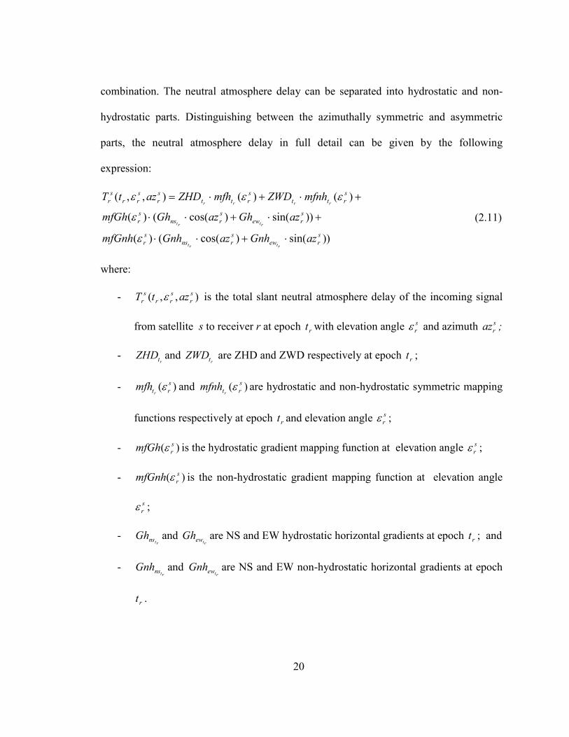
20

combination. The neutral atmosphere delay can be separated into hydrostatic and non-

hydrostatic parts. Distinguishing between the azimuthally symmetric and asymmetric

parts, the neutral atmosphere delay in full detail can be given by the following

expression:

))sin()cos(()(

))sin()cos(()(

)()(),,(

s

rew

s

rns

s

r

s

rew

s

rns

s

r

s

rtt

s

rtt

s

r

s

rr

s

r

azGnhazGnhmfGnh

azGhazGhmfGh

mfnhZWDmfhZHDaztT

rtrt

rtrt

rrrr

⋅+⋅⋅

+⋅+⋅⋅

+⋅+⋅=

ε

ε

εεε

(2.11)

where:

- ),,( s

r

s

rr

s

r aztT ε is the total slant neutral atmosphere delay of the incoming signal

from satellite s to receiver r at epoch rt with elevation angle s

rε and azimuth s

raz ;

- rt

ZHD and rt

ZWD are ZHD and ZWD respectively at epoch rt ;

- )( s

rtrmfh ε and )( s

rtrmfnh ε are hydrostatic and non-hydrostatic symmetric mapping

functions respectively at epoch rt and elevation angle s

rε ;

- )( s

rmfGh ε is the hydrostatic gradient mapping function at elevation angle s

rε ;

- )( s

rmfGnh ε is the non-hydrostatic gradient mapping function at elevation angle

s

rε ;

- rt

nsGh and rt

ewGh are NS and EW hydrostatic horizontal gradients at epoch rt ; and

- rt

nsGnh and rt

ewGnh are NS and EW non-hydrostatic horizontal gradients at epoch

rt .

21

For high precision applications and when low elevation angle measurements are used, the

estimation of gradients has been suggested (see e.g. Meindl et al. [2004], Emardson and

Jarlemark [1999], Bar-Sever et al. [1998] and Chen and Herring [1997]). Equation (2.11)

includes separated hydrostatic and non-hydrostatic gradient components. These probably

can not be estimated separately in the parameter estimation process [Chen and Herring,

1997] due to the increased number of unknown parameters. Hence a more practical

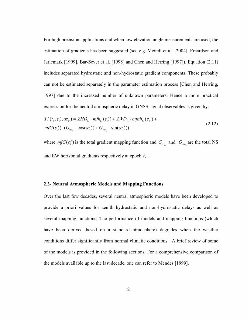
expression for the neutral atmospheric delay in GNSS signal observables is given by:

))sin()cos(()(

)()(),,(s

rew

s

rns

s

r

s

rtt

s

rtt

s

r

s

rr

s

r

azGazGmfG

mfnhZWDmfhZHDaztT

rtrt

rrrr

⋅+⋅⋅

+⋅+⋅=

ε

εεε (2.12)

where )( s

rmfG ε is the total gradient mapping function and rt

nsG and rt

ewG are the total NS

and EW horizontal gradients respectively at epoch rt .

2.3- Neutral Atmospheric Models and Mapping Functions

Over the last few decades, several neutral atmospheric models have been developed to

provide a priori values for zenith hydrostatic and non-hydrostatic delays as well as

several mapping functions. The performance of models and mapping functions (which

have been derived based on a standard atmosphere) degrades when the weather

conditions differ significantly from normal climatic conditions. A brief review of some

of the models is provided in the following sections. For a comprehensive comparison of

the models available up to the last decade, one can refer to Mendes [1999].

22

2.3.1- Zenith Hydrostatic (and Dry) Delay Models

Hopfield [1969] derived a dry delay model based on a refractivity model. Saastamoinen

[1972a, 1972b, 1973] and Baby et al. [1988] developed hydrostatic delay models based

upon a theoretical definition of hydrostatic delay and a hydrostatic equilibrium

assumption. Later, Davis et al. [1985] slightly improved the Saastamoinen model. These

hydrostatic delay models differ due to the choice of the refractivity constant and on the

modelling of the height and latitude dependence of gravity acceleration [Mendes, 1999]

but all follow the same theoretical procedures. Mendes [1999] concluded that zenith

hydrostatic delay can be predicted from surface pressure measurements with a total error

below 5 mm and concluded that of the mentioned models, the Saastamoinen model

performance is far better than the other hydrostatic models. This conclusion was based on

the fact that predictions obtained with this model agreed with his ray tracing results at the

sub-millimetre level whereas the other models agreed at the millimetre level.

2.3.2- Zenith Non-Hydrostatic (and Wet) Delay Models

Due to the difficulty of modelling the water vapour profile, there are more models for the

zenith non-hydrostatic and wet delay than for the hydrostatic delay. Mendes [1999]

compared a number of these models and concluded that the Ifadis [1986] and

Saatamoinen [1972a, 1972b, 1973] models have better performance. However, it was

mentioned that these models are highly correlated. It was also mentioned that the zenith

23

non-hydrostatic delay cannot be predicted using surface meteorological values to an

accuracy of better than a few centimetres.

2.3.3- Mapping Functions

A large number of mapping functions have been developed. These are either total

mapping functions or purely hydrostatic and non-hydrostatic functions. Recent mapping

functions are usually based on the truncated form of a continued fraction. Mendes [1999]

carried out a comprehensive comparison among the mapping functions developed up to

1996 and concluded that Ifadis [1986], MTT [Herring, 1992] and Niell [1996] hydrostatic

and non-hydrostatic mapping functions perform best. In general, the Niell mapping

function (which is independent of meteorological measurements) was recommended.

This mapping function has been widely used in GPS software. However, studies by Niell

and Petrov [2003] indicate that use of the hydrostatic Niell mapping function for

elevation angles below 10 degrees significantly increases the height uncertainty. Guo

and Langley [2003] developed a mapping function for elevation angles down to 2 degrees

(namely UNBabc) and recommended it for a GNSS receiver built-in mapping function

due to its simplicity with respect to Niell mapping functions.

In order to overcome some of the detected biases due to missmodelling of the

meteorological parameters and also the fact that mapping functions like Niell are not

based on real-time parameters, some recent mapping functions use information from

24

NWP models. In Chapter 3 new symmetric mapping functions based on NWP models as

well as gradient mapping functions are explained and compared.

2.3.4- Modeling the Meteorological Parameters

Most of the zenith delay models and some mapping functions need measurements of

surface meteorological parameters. However, most users do not have access to such data.

Due to this fact a number of studies have been carried out on the subject of modelling the

meteorological parameters.

Collins [1999] developed a number of tropospheric models for aircraft users of GPS.

Among those, the UNB3 model has been widely used for many GPS applications. The

UNB3 model is the basis for the RTCA, Inc. (formerly, Radio Technical Commission for

Aeronautics) satellite-based augmentation system minimum operational performance

standards neutral atmosphere delay model [RTCA, 2006], which is used for the Wide

Area Augmentation System, the European Geostationary Navigation Overlay Service,

and other satellite-based augmentation systems. This model is based on the works of

Saastamoinen [1972a, 1972b, 1973] and Niell [1996] for zenith delay and mapping

functions respectively. A look-up table of atmospheric parameters based on the 1966 U.S.

Standard Atmosphere is used in the UNB3 model. The model input parameters are day

of year, elevation angle, height and latitude. UNB3m [Orliac, 2002; Leandro et al., 2008]

improves on UNB3 through an improved handling of the wet delay.

25

Schüler et al. [2001] proposed a tropospheric correction model namely GTN (Global

Tropospheric Navigation model). In contrast to UNB3, this model not only includes a

latitudinal correction data field, but also a longitudinal one with a higher horizontal

resolution which accounts for regional variations. The GTN models were derived from

analyses of GDAS (Global Data Assimilation System) numerical weather fields.

Leandro et al. [2006] developed a wide area neutral atmosphere model for North America

(namely UNBw.na). They reported that the new grid-based model could perform better

than models based only on latitude (such as UNB3m) even though the improvement may

not be spectacular.

Boehm et al. [2007a] developed a global model of pressure and temperature for geodetic

applications namely GPT (Global Pressure and Temperature). GPT is based on spherical

harmonics up to degree and order nine and provides pressure and temperature for any site

at or near the Earth’s surface. This model was derived from 3 years of 15°×15° global

grids of monthly mean profiles for pressure and temperature from the ECMWF 40 years

reanalysis data.

2.4- Summary

In this chapter, theoretical aspects of neutral atmosphere effects on GNSS signals have

been addressed. Some zenith delay models and mapping functions have also been briefly

reviewed. One may refer to e.g. Mendes [1999] for a more comprehensive theoretical

26

background and historical review of the older models. In Chapter 3 recent developments

in mapping functions based on NWP models as well as gradient mapping functions will

be discussed in detail.

27

3. Chapter 3: Recent Developments in Neutral Atmosphere

Mapping Functions

In this chapter recent mapping functions based on NWP models as well as commonly

used gradient mapping functions are reviewed. Older mapping functions which were not

based on (or derived from) NWP model data have been compared and reviewed

comprehensively by Mendes [1999]. However, as mentioned in the previous chapter,

among older mapping functions, Niell [1996] is still being used by many software

products and analysis centres and is relevant for introducing the newer mapping

functions. Hence, in this chapter, in addition to newer mapping functions based on NWP

models, the Niell mapping functions are also reviewed.

3.1- Recent Symmetric Mapping Functions

3.1.1- Niell Mapping Functions

Niell mapping functions (NMF) use the continued fractional form as presented first by

Marini [1972] as follow:

++

+

++

+

−⋅+

++

+

++

+

= −

ht

ht

ht

ht

ht

ht

s

i

i

i

i

i

i

i

c

b

a

c

b

a

H

c

b

a

c

b

a

m

εε

εε

εε

εε

sinsin

sin

11

1

sin

110

sinsin

sin

11

1

)( 3

(3.1)

28

where ε is the vacuum (unrefracted) elevation angle and i is replaced by h or nh standing

for hydrostatic and non-hydrostatic respectively. The second term of the above equation,

in which sH is the orthometric height of the station in metres, is a height correction term

and only applied to the hydrostatic mapping function. The ht terms for the height

correction part are:

553.2 −= eaht (3.2.a)

349.5 −= ebht (3.2.b)

314.1 −= echt (3.2.c)

The coefficients for the hydrostatic part are functions of the station latitude and day of

year as follow1:

−−=

25.365

282cos)()(),(

DoYaaDoYa ihihih ampavg

πϕϕϕ (3.3.a)

−−=

25.365

282cos)()(),(

DoYbbDoYb ihihih ampavg

πϕϕϕ (3.3.b)

−−=

25.365

282cos)()(),(

DoYccDoYc ihihih ampavg

πϕϕϕ (3.3.c)

where coefficients with subscripts avg and amp are determined for the five latitudes as

presented in Table 3.1 and are obtained by linear interpolation for non-tabulated latitudes.

1 Note that these equations are the corrected ones as oppose to some earlier publications in which the two terms in the equations were added together.

29

Parameters for latitudes from 0 to 15° are the same as those for 15°. Parameters for

latitudes above 75° are also the same as those for 75°. The mapping function is

symmetric with respect to the equator except for the coefficients in equations (3.3) in

which a phase of π is added for the southern hemisphere to account for seasonal

differences.

Table 3.1- Coefficients for NMF

Latitude Coeff. 15° 30° 45° 60° 75°

avgha 32769934.1 −e 32683230.1 −e 32465397.1 −e 32196049.1 −e 32045996.1 −e

avghb 39153695.2 −e 39152299.2 −e 39288445.2 −e 39022565.2 −e 39024912.2 −e

avghc 3610505.62 −e 3837393.62 −e 3721774.63 −e 3824265.63 −e 3258455.64 −e

aampha 0 52709626.1 −e 56523662.2 −e 54000452.3 −e 51202191.4 −e

aamphb 0 51414979.2 −e 50160779.3 −e 52562722.7 −e 5723375.11 −e

aamphc 0 50128400.9 −e 53497037.4 −e 5795348.84 −e 537206.170 −e

nha 48021897.5 −e 46794847.5 −e 48118019.5 −e 49727542.5 −e 41641693.6 −e

nhb 34275268.1 −e 35138625.1 −e 34572752.1 −e 35007428.1 −e 37599082.1 −e

nhc 23472961.4 −e 26729510.4 −e 23908931.4 −e 24626982.4 −e 24736038.5 −e

The popularity of NMF apart from higher accuracy than the older mapping functions is

due to the fact that it does not require meteorological parameters and hence is rather easy

to use. As an example, NMF values at day of year 182 for 5 degree elevation angle for

the whole world have been calculated at the surface grid points of the global high

resolution Canadian NWP model and presented at Figures 3.1 and 3.2.

30

Figure 3.1– Hydrostatic NMF at 5 degree elevation angle on DoY 182 calculated on all grid points of the

Canadian high resolution global NWP model

Figure 3.2– Non-hydrostatic NMF at 5 degree elevation angle calculated on all grid points of the Canadian

high resolution global NWP model

31

While NMF has been a popular mapping function in the GNSS community, it suffers

from some systematic biases mainly in the southern hemisphere (see section 3.1.5 and

Chapter 6). As can be seen in Figure 3.2, the non-hydrostatic NMF is symmetric with

respect to the equator. It should also be mentioned that the non-hydrostatic NMF is not

dependent on day of year and hence what is represented in Figure 3.2 are mapping factor

values for any epoch. Apart from a height correction, the hydrostatic NMF differs

between northern and southern hemispheres by a phase change in the coefficients (as

mentioned before in equations (3.3)).

3.1.2- Isobaric Mapping Functions

Niell [2000] proposed new mapping functions based on parameters from numerical

weather models, namely Isobaric Mapping Functions (IMF). He studied the correlation of

isobaric heights with radiosonde-derived hydrostatic mapping functions and reported that

the 200 hPa level shows the highest correlation with the mapping function at 5°. Similar

to NMF a continued fraction with three coefficients was adopted as follows:

c

b

ac

b

a

m

++

+

++

+

=

εε

εε

sinsin

sin

11

1

)( (3.4)

32

The coefficients for the hydrostatic mapping function are as follows (Niell [2003]):

)( 200 rzzaa −⋅+= ϕϕ ζ (3.5.a)

002905.0=b (3.5.b)

)cos(0014.00634.0 ϕ⋅+=c (3.5.c)

where:

))2(2cos(00004.000124.0 −⋅⋅+= ϕϕa (3.6.a)

)2cos(000000016.0000000074.0 ϕζ ϕ ⋅−= (3.6.b)

))3(2cos(61911836 −⋅⋅+= ϕrz (3.6.c)

where ϕ and 200z are the latitude and height of the 200 hPa level above the site. A height

correction similar to the one for NMF should also be applied here.

The coefficients for the non-hydrostatic (wet) mapping function are as follows (Niell

[2003]):

)0000001658.000068827.000020795.0()5.15( 3 hmfa ⋅−+−⋅−= (3.7.a)

0013503.000018882.0)5.15( 3 +⋅−= mfb (3.7.b)

0039647.00048581.0)5.15( 3 +⋅−= mfc (3.7.c)

where 3mf is the mapping function at 3° elevation calculated using ray tracing of

numerical weather model grids and h is the height of the site.

33

As an example, the hydrostatic IMF at 5 degree elevation angle has been calculated at all

grid points of the Canadian global high resolution NWP model at DoY 182, 2008 and are

presented in Figure 3.3.

Figure 3.3 – Hydrostatic IMF at 5 degree elevation angle on DoY 182 calculated on all grid points of


3.1.3- Vienna Mapping Functions

Vienna mapping functions (VMF) introduced by Boehm and Schuh [2004] use the b and

c coefficients of IMF for the hydrostatic part, and those of NMF at 45° latitude for the

non-hydrostatic part (i.e.: 04391.0,00146.0 == nhnh cb ). Ray tracing with an initial

elevation angle of 3.3° is carried out and by inverting the continued fraction form the a

coefficients can be determined as follow:

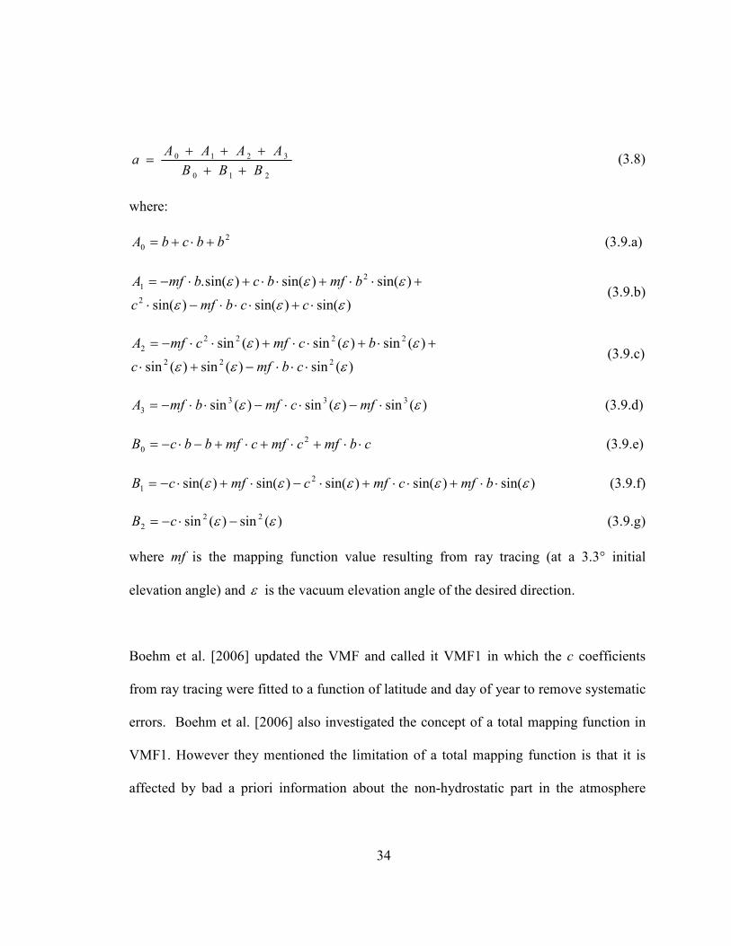
34

210

3210

BBB

AAAAa

+++++

= (3.8)

where:

20 bbcbA +⋅+= (3.9.a)

)sin()sin()sin(

)sin()sin()sin(.2

21

εεε

εεε

⋅+⋅⋅⋅−⋅

+⋅⋅+⋅⋅+⋅−=

ccbmfc

bmfbcbmfA (3.9.b)

)(sin)(sin)(sin

)(sin)(sin)(sin222

22222

εεε

εεε

⋅⋅⋅−+⋅

+⋅+⋅⋅+⋅⋅−=

cbmfc

bcmfcmfA (3.9.c)

)(sin)(sin)(sin 3333 εεε ⋅−⋅⋅−⋅⋅−= mfcmfbmfA (3.9.d)

cbmfcmfcmfbbcB ⋅⋅+⋅+⋅+−⋅−= 20 (3.9.e)

)sin()sin()sin()sin()sin( 21 εεεεε ⋅⋅+⋅⋅+⋅−⋅+⋅−= bmfcmfcmfcB (3.9.f)

)(sin)(sin 222 εε −⋅−= cB (3.9.g)

where mf is the mapping function value resulting from ray tracing (at a 3.3° initial

elevation angle) and ε is the vacuum elevation angle of the desired direction.

Boehm et al. [2006] updated the VMF and called it VMF1 in which the c coefficients

from ray tracing were fitted to a function of latitude and day of year to remove systematic

errors. Boehm et al. [2006] also investigated the concept of a total mapping function in

VMF1. However they mentioned the limitation of a total mapping function is that it is

affected by bad a priori information about the non-hydrostatic part in the atmosphere

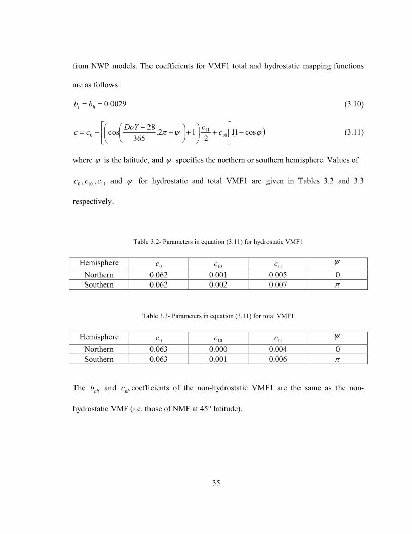
35

from NWP models. The coefficients for VMF1 total and hydrostatic mapping functions

are as follows:

0029.0== ht bb (3.10)

( )ϕψπ cos1.2.12.

365

28cos 10

110 −

+

+

+−

+= ccDoY

cc (3.11)

where ϕ is the latitude, and ψ specifies the northern or southern hemisphere. Values of

0c , 10c , 11c and ψ for hydrostatic and total VMF1 are given in Tables 3.2 and 3.3

respectively.

Table 3.2- Parameters in equation (3.11) for hydrostatic VMF1

Hemisphere 0c 10c 11c ψ

Northern 0.062 0.001 0.005 0 Southern 0.062 0.002 0.007 π

Table 3.3- Parameters in equation (3.11) for total VMF1

Hemisphere 0c 10c 11c ψ

Northern 0.063 0.000 0.004 0 Southern 0.063 0.001 0.006 π

The nhb and nhc coefficients of the non-hydrostatic VMF1 are the same as the non-

hydrostatic VMF (i.e. those of NMF at 45° latitude).

36

3.1.4- Global Mapping Functions

Boehm et al. [2006] developed Global Mapping Functions (GMF), using 15°×15° global

grids of monthly mean profiles from pressure, temperature, and humidity from the

ECMWF 40 years reanalysis data (the same data that was used for GPT, see Chapter 2).

This mapping function takes empirical equations for b and c from VMF1 and the

coefficient a is calculated from spherical harmonics on a global grid from the following

equations:

⋅−

⋅+= π2365

28cos0

DoYAaa (3.12)

where:

)]sin().cos([)(sin9

0 00 λλϕ ⋅⋅+⋅⋅⋅=∑∑

= =

mBmAPa nm

n

n

m

nmnm (3.13)

where DoY is day of year, 0a is the global grid of mean values, A are the annual

amplitudes, )(sinϕnmP are the Legendre associated functions of n degree and m order,

and nmA and nmB are the spherical harmonic coefficients.

Unlike VMF1, which requires real-time NWP data, GMF only requires station

coordinates and day of year. As an example, hydrostatic and non-hydrostatic GMF for

DoY 182 at 5 degree elevation angle are presented at Figures 3.4 and 3.5 respectively.

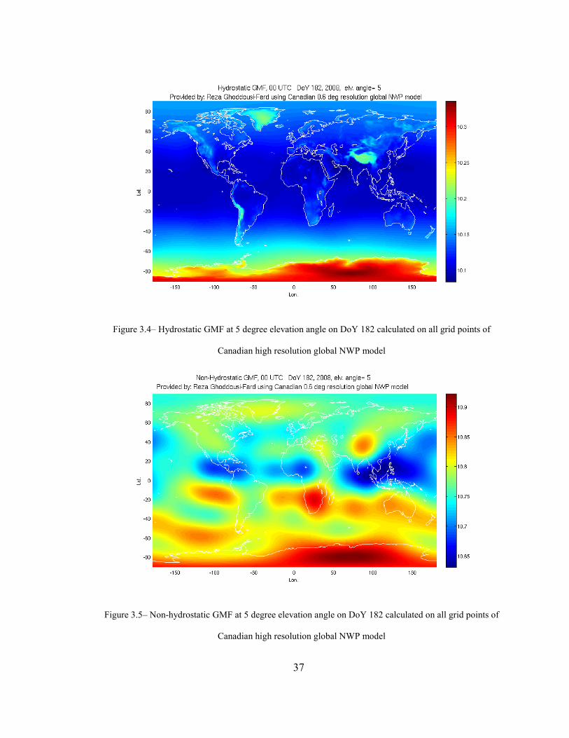
37

Figure 3.4– Hydrostatic GMF at 5 degree elevation angle on DoY 182 calculated on all grid points of


Figure 3.5– Non-hydrostatic GMF at 5 degree elevation angle on DoY 182 calculated on all grid points of


38

3.1.5- Comparison of Recent Symmetric Mapping Functions

As mentioned before, while VMF1 and IMF are partly based on ray tracing through NWP

models, NMF and GMF are empirical mapping functions and do not require real-time

data. Hence, among these mapping functions, NMF followed by GMF are easiest to use

but they are not tuned to day-to-day weather variations. In this regard, VMF1 and IMF

have the advantage. What is practically of interest to the GNSS community is how much

change in slant delay might arise as a result of using one mapping function as opposed to

the other (as well as how easy they are to use).

The differences between hydrostatic and non-hydrostatic GMF and NMF at DoY 182 at 5

degree elevation angle are presented at Figures 3.6 and 3.7.

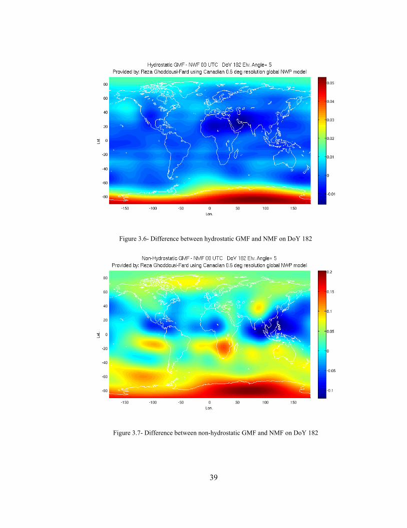
39

Figure 3.6- Difference between hydrostatic GMF and NMF on DoY 182

Figure 3.7- Difference between non-hydrostatic GMF and NMF on DoY 182

40

The differences shown in the above maps are multiplied by ZHD and ZWD from the

Canadian global NWP model at the same epoch in 2008 and the results are the

differences that these two mapping functions cause in slant delay. These are presented in

Figures 3.8 and 3.9.

Figure 3.8- Difference between slant hydrostatic delays resulting from GMF and NMF on DoY 182, 2008

41

Figure 3.9- Difference between slant non-hydrostatic delays resulting from GMF and NMF on DoY 182,

2008

Since ZHD is one order of magnitude larger than ZWD, despite the smaller difference

between hydrostatic mapping function values compared to non-hydrostatic (Figures 3.6

and 3.7), the resulting slant hydrostatic delay differences due to using GMF instead of

NMF is larger than the slant non-hydrostatic delay. As can be seen in Figure 3.8 the use

of GMF instead of NMF can cause up to about 10 cm slant hydrostatic delay difference at

5 degree elevation angle while the maximum slant non-hydrostatic delay difference in the

investigated day is about 5 cm.

Figure 3.10 shows the slant hydrostatic delay differences at 5 degree elevation angle as a

result of using IMF instead of NMF on the same day as above. Apart from large biases in

42

Antarctica which were also visible in Figure 3.8 (GMF vs. NMF), local anomalies also

have caused differences of a few centimetres on the investigated day.

Figure 3.10- Difference between slant hydrostatic delays resulting from IMF and NMF on DoY 182, 2008

Based on the actual GPS constellation, slant delay differences as a result of changing

mapping function are investigated. In all cases the mapping function differences are

multiplied by the zenith delay from the global high resolution Canadian NWP model

interpolated at each epoch (every 30 seconds) to present the results in units of delay

(metre). One can see the differences of slant hydrostatic delay between the mapping

functions mentioned in the previous sections at station ALGO, Canada over 24 hours on

DoY 197, 2007 in Figures 3.11. The maximum difference and percentages of values

larger than 1 cm with respect to the whole measurements over the day are quoted in the

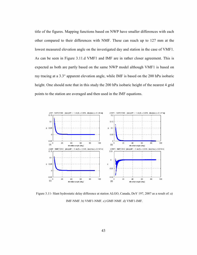
43

title of the figures. Mapping functions based on NWP have smaller differences with each

other compared to their differences with NMF. These can reach up to 127 mm at the

lowest measured elevation angle on the investigated day and station in the case of VMF1.

As can be seen in Figure 3.11.d VMF1 and IMF are in rather closer agreement. This is

expected as both are partly based on the same NWP model although VMF1 is based on

ray tracing at a 3.3° apparent elevation angle, while IMF is based on the 200 hPa isobaric

height. One should note that in this study the 200 hPa isobaric height of the nearest 4 grid

points to the station are averaged and then used in the IMF equations.

Figure 3.11- Slant hydrostatic delay difference at station ALGO, Canada, DoY 197, 2007 as a result of: a)

IMF-NMF. b) VMF1-NMF. c) GMF-NMF. d) VMF1-IMF.

44

Similarly, slant non-hydrostatic delay between the mapping functions mentioned in the

previous sections at station ALGO, Canada over 24 hours on DoY 197, 2007 are

presented in Figures 3.12. As mentioned earlier, despite larger uncertainties in non-

hydrostatic mapping functions in general, the slant non-hydrostatic delay differences are

smaller due to the smaller ZWD compared to ZHD. The exception is the difference

between non-hydrostatic VMF1 and IMF which is larger compared to hydrostatic values.

The formulation of non-hydrostatic coefficients in IMF is derived from equations (3.7),

while VMF1 is similar to NMF in the cases of nhb and nhc but nha is based on ray

tracing.

Figure 3.12– Slant non-hydrostatic delay difference at station ALGO, Canada, DoY 197, 2007 as a result

of: a) IMF-NMF b) VMF1-NMF c) GMF-NMF d) VMF1-IMF

45

IERS Conventions Update [2007] (based on validation results of Niell [2006], Boehm

[2007b] and Tesmer et al. [2007]) has recommended VMF1 for any global application,

such as the determination of the terrestrial reference frame and Earth orientation

parameters. As expected, and as it is clear in Figures 3.11 and 3.12, the choice of

mapping function affects the slant delays significantly only at elevation angles below 15-

20 degrees.

3.2- Gradient Models and Mapping Functions

Compared to the models and mapping functions used for the symmetric atmosphere,

there are not many gradient models and mapping functions developed for the asymmetric

part. In this section common gradient models and mapping functions are reviewed. A

hydrostatic gradient model derived as a part of this dissertation research work will be

introduced in Chapter 5.

Similar to the common approach to deal with the symmetric part of the delay, the use of

an elevation-dependent function to map the horizontal azimuthally dependent delays has

also been used to model the asymmetric part. The geodetic azimuth (α ) and elevation

angle (ε ) between two points (with geometric distance S) can be related to local geodetic

coordinate system as follows:

αε coscos ⋅⋅= SN (3.13.a)

46

αε sincos ⋅⋅= SE (3.13.b)

εsin⋅= Sh (3.13.c)

where N, E and h are north, east and height components respectively. From equations

(3.13) the position vector of a point on the path can be written as follows:

)sin(coscot),( enhx))r⋅+⋅⋅⋅≅ ααεαε (3.14)

where n and e are the unit vectors to the north and east respectively.

Equation (3.14) is the basis of available gradient models which will be reviewed in the

following sections.

3.2.1- Davis et al.

Based on the above relations, Davis et al. [1993] (with the assumption of linear variation

of refractivity with horizontal distance) defined a gradient model as follows:

)sincos(cot)(),( ααεεαε ⋅+⋅⋅′⋅= ENsymasym GGmd (3.15)

where )(εsym

m is a symmetric mapping function (i.e. not a function of azimuth), ε ′ is the

refracted elevation angle, and N

G and E

G are the delay gradients in the north and east

directions respectively. Using an approximate relation between the refracted and

unrefracted (vacuum) elevation angle given by Bean and Dutton [1966], the Davis

gradient model in equation (3.15) is given as:

)sincos()csc101(cot)(),( 26 ααεεεαε ⋅+⋅⋅⋅−⋅⋅≅ −ENssymasym GGNmd (3.16)

47

where s

N is the total surface refractivity.

Later, MacMillan [1995] and MacMillan and Ma [1997] applied the gradient model of

Davis in VLBI analysis (by replacing ε ′ simply by ε in equation (3.15)) and noted that

the results are not sensitive to whether )(εsym

m is replaced by a hydrostatic or non-

hydrostatic mapping function.

3.2.2- Chen and Herring

Chen and Herring [1997] showed that the gradient mapping function can be expressed

approximately as a continued fraction expansion in the form of εε tan.sin i.e.:

...tansintansin

tansin

1)(

2

1

++

+=

εεεε

εεε

c

cmasym (3.17)

They have retained just the first term i.e.:

Cmasym +⋅

=εε

εtansin

1)( (3.18)

where:

∫∫

+⋅∇

⋅∇=

dhRhhN

dhhNC

)(2

3 2

(3.19)

where N∇ is the gradient of refractivity, h is the height and R is the radius of Earth.

Under the assumption of an exponential decay in the gradient with scale height of sH ,

48

equation (3.19) reduces to R

H s

2

3 [Chen and Herring, 1997]. Hence assuming a hydrostatic

gradient scale height of 13 km, and radius of the Earth equal to 6370 km, C = 0.0031. For

a non-hydrostatic gradient scale height of 3 km, C=0.0007. However, Chen and Herring

[1997] used a combined value of 0.0032 in their VLBI analysis as it is difficult to

estimate the hydrostatic and non hydrostatic parts separately.

In order to use the Chen and Herring asymmetric mapping function, one may replace the

εε ′cot).(sym

m term in equation (3.15) with equation (3.18).

3.2.3- Tilting of the Atmosphere

Tilting the zenith direction in the mapping function by a small angle β may represent a

tropospheric gradient (see e.g. Meindl et al. [2004]). The geometry of tilting the zenith

direction is represented in Figure 3.13. In Figure 3.13 the tropospheric zenith is defined

as normal to the tilted atmosphere while the geometric zenith is defined as normal to the

untilted (symmetric) atmosphere. Based on the representation in Figure 3.13 and

according to the first spherical law of cosines, we may write:

)cos()sin()sin()cos()cos()ˆcos( 0AAzzz −+= ββ (3.20)

where A is the azimuth of the observation, 0A is the azimuth of the tropospheric zenith

direction ( z ) with respect to the geometric zenith direction (z).

Since β is small we may write:

49

ββ ≅)sin( and 1)cos( ≅β

From equation (3.20) and considering a small value for β [Meindl et al., 2004] and

assuming:

zzz δ+=ˆ (3.21)

we can write:

)cos()sin()cos()cos( 0AAzzzz −+=+ βδ (3.22)

or:

)cos()sin()cos()sin()sin()cos()cos( 0AAzzzzzz −+=− βδδ . (3.23)

Since zδ is small we may write:

)cos()sin()cos()sin()cos( 0AAzzzzz −+=− βδ (3.24)

which results in:

)cos( 0AAz −−= βδ (3.25)

From (3.21) and (3.25) we can write:

)cos(ˆ 0AAzz −−= β (3.26)

By defining: )cos( 0Ax β−= and )sin( 0Ay β−= we can write:

)sin()cos(ˆ AyAxzz ++= (3.27)

hence:

)sin()cos(ˆ AyAxzzz +==− δ (3.28)

Following (3.21), )()ˆ( zzfzf δ+= and by a linear approximation (using Taylor’s

theorem) we may write:

50

zz

fzfzzz

z

fzfzf δδ

∂∂

+=−+∂∂

+= )()()()ˆ( (3.29)

and considering (3.28) finally we have:

)sin()cos()()ˆ( Ayz

fAx

z

fzfzf

∂∂

+∂∂

+= (3.30)

Figure 3.13- Geometry of spherical triangle as a result of tilting the zenith direction

Assuming a simple mapping function of εsin

1=f equation (3.30) can be expressed in a

similar form as equation (3.15).

51

3.2.4- Niell Hydrostatic Gradient Mapping Function

Niell [2001] proposed a hydrostatic gradient mapping function based on the same idea

used in the IMF. Therefore this mapping function requires access to information from

NWP models. The tilt of the hydrostatic atmosphere is defined as the direction of the

normal to the surface defined by the geopotential height of the 200 hPa surface at the four

nearest grid points. This direction is represented by gradient azimuth ( gα ) and gradient

zenith angle ( gz ). The form of this mapping function is as follows:

))cos((),,( gggg zMFhzGMFh αεαε ⋅−= (3.31)

where GMFh is the hydrostatic gradient mapping function, MFh is an arbitrary

azimuthally symmetric hydrostatic mapping function, and ε is the elevation angle of an

observation. Following Niell [2003] the gradient azimuth and gradient zenith angle may

be estimated by satisfying the following equation:

0)( 0 =−⋅ XWh m

rrr (3.32)

where [ ]zyx hhhh =r

is the normal to the plane that is fitted to 200 hPa geopotential

heights at the grid points,

=

mz

my

mx

m

w

w

w

Wr

is the position vector of the 200 hPa geopotential

surface at the grid points, and

=

x

x

x

z

y

x

X

0

0

0

0

r is the position vector of the 200 hPa

geopotential surface above the site.

52

From (3.32) one can derive the z component as follows:

)()( 000 ymy

z

y

xmx

z

xzmz xw

h

hxw

h

hxw −−−−= (3.33)

Since the normal vector is a unit vector, only the ratios of the components need to be

estimated. Hence the vector of unknowns is defined as:

[ ]yzxzz hhxy 0=r

, where z

x

xzh

hh = and

z

y

yzh

hh = .

The vector of observations is composed of the z component of the position vector of grid

points.

A weighted least-squares approach can be used for estimation of the unknowns, where

weights are calculated from the uncertainty in 200 hPa geopotential heights. The gradient

azimuth ( gα ) and gradient zenith angle ( gz ) finally can be calculated in units of degrees

by:

),(2tan180

yzxzg hha⋅=π

αo

(3.34)

),1(2tan180

90 xyg raz ⋅−=π

o

o (3.35)

where ( ) 2/122yzxzxy hhr += and atan2 is the four-quadrant inverse tangent function.

53

3.3- Summary

Comparison between recent mapping functions carried out in this chapter shows up to

more than 10 cm difference between the NWP-based mapping functions and the NMF in

low elevation angle measurements. Some of the symmetric and gradient mapping

functions discussed in this chapter will be used later throughout this dissertation either for

implementation in GPS software or in validation studies.

54

4. Chapter 4: Ray Tracing: Theory and Practice

In this chapter, the ray tracing algorithm developed for this research is reviewed. A web-

based ray tracing package, accessible to the public and developed as a part of this

research, will be discussed. Validation of data sources used in ray tracing in different

locations and using different sensors - including surface met sensors and a water vapour

radiometer (WVR) - will be addressed as well.

4.1- Ray Tracing: A Review

According to the American Meteorological Society’s Glossary of Meteorology [AMS,

2007], ray tracing is:

“a graphical or mathematical approximation scheme for determining the propagation of

electromagnetic or sound waves by following the path of rays obeying the laws of

reflection and refraction.” Ray tracing has been a common approach for dealing with radio signal propagation

through the atmosphere for a long time (see, e.g., Bean and Dutton [1966]). The term

“ray tracing” is also used in other disciplines such as geophysics (see, e.g., Rucker and

Ferré [2004]).

In order to estimate the delay along the signal path, numerical integration requires a

series of thin spherical layers within which a constant refractivity is assumed. Assuming a

symmetric atmosphere around a GNSS receiver, these layers are made by using vertical

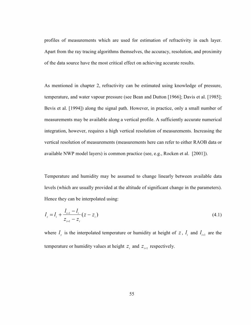
55

profiles of measurements which are used for estimation of refractivity in each layer.

Apart from the ray tracing algorithms themselves, the accuracy, resolution, and proximity

of the data source have the most critical effect on achieving accurate results.

As mentioned in chapter 2, refractivity can be estimated using knowledge of pressure,

temperature, and water vapour pressure (see Bean and Dutton [1966]; Davis et al. [1985];

Bevis et al. [1994]) along the signal path. However, in practice, only a small number of

measurements may be available along a vertical profile. A sufficiently accurate numerical

integration, however, requires a high vertical resolution of measurements. Increasing the

vertical resolution of measurements (measurements here can refer to either RAOB data or

available NWP model layers) is common practice (see, e.g., Rocken et al. [2001]).

Temperature and humidity may be assumed to change linearly between available data

levels (which are usually provided at the altitude of significant change in the parameters).

Hence they can be interpolated using:

)(1

1i

ii

ii

izzz

zz

llll −

−−

+=+

+ (4.1)

where zl is the interpolated temperature or humidity at height of z ,

il and 1+il are the

temperature or humidity values at height i

z and 1+iz respectively.

56

Assuming an isothermal atmosphere (dry atmosphere of constant temperature) in

hydrostatic equilibrium (see, e.g., Andrews [2000]), pressure values can be interpolated

by using the following equations:

)~(

0

)(

00 H

z

TR

gz

ePePP d

−−

== , (4.2a)

where

%H =RdT0

g (4.2b)

In the above equations, P is the pressure at height z above the surface, P0 is the surface

pressure (or pressure at adjacent level), T0 is surface temperature (or temperature at

adjacent level), Rd is the specific gas constant for dry air, and g is the gravity acceleration

that changes slightly with latitude and height (less than 1% for a height change of 30 km

or latitude difference of 1 degree). One may refer to Marini and Murray [1973] and List

[1966] for a gravity model that uses an effective Earth radius and height. %H is called

“pressure scale height” (the height over which the pressure decreases by a factor of e). If

the temperature is known as a function of height (e.g., at each level), the above equations

may be used to find the pressure as a function of height. For moist air, virtual temperature

(see, e.g., Wallace and Hobbs [1977]) rather than actual temperature should be used in

equations (4.2a) and (4.2b).

The vertical interpolation approaches mentioned above are also used to derive surface

values when the user (GPS antenna) height is not the same as the surface height of the

meteorological profile. Some unavoidable errors in the determination of ZTD exist due to

the vertical interpolation (or extrapolation, where the data source surface level is higher

57

than the GPS antenna). Exponential pressure interpolation is known to have a very good

agreement with the vertical profile of the pressure. However, the temperature (and

humidity measure) is interpolated linearly. This might be erroneous when there is a large

height difference between the surface level of the data source and the GPS antenna.

When there is temperature inversion1, for example, the aforementioned issue might be of

more concern. Figure 4.1 shows the vertical profile of temperature at station WHIT

(YXY) in Whitehorse, Yukon, where a large height difference between GPS and

radiosonde surface measurements exists (over 700 m). A zoomed view of the lower levels

can be seen in Figure 4.2 where the GPS antenna level and radiosonde surface

measurement have also been shown. The interpolated temperature values above the

height of the GPS antenna do not consider any inversion layer (which may be incorrect).

However, temperature errors are less important than pressure errors in ZTD

determination and could be insignificant when compared to errors due to other

assumptions.

In the ray tracing package developed as part of this dissertation research, the resolution of

meteorological parameters was increased by using a step size of 10 m from the surface up

to the altitude of 20 km and 50 m from 20 km to the top of the neutral atmosphere. Figure

4.3 shows the effect of changing the ray tracing integration step size for slant total delay

1 Layers of air with negative lapse rates, i.e. where temperatures increases with height. Temperature inversion is a frequent phenomenon in the Arctic. The Arctic temperature inversion is usually because of snow and ice surfaces that exist in the Arctic regions. This low-level inversion is present almost continuously over the Arctic in winter and over snow and ice covered areas in summer [Maxwell, 1982].

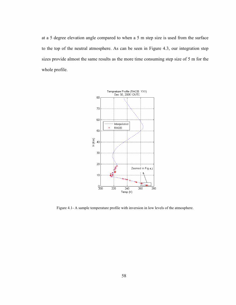
58

at a 5 degree elevation angle compared to when a 5 m step size is used from the surface

to the top of the neutral atmosphere. As can be seen in Figure 4.3, our integration step

sizes provide almost the same results as the more time consuming step size of 5 m for the

whole profile.

Figure 4.1- A sample temperature profile with inversion in low levels of the atmosphere.

59

Figure 4.2- A Closer view at lower levels of Fig. 4.1.

Figure 4.3- Effect of changing the integration step size for 5 degree slant total delay ray tracing result

compared to a step sizes of 5 m for the whole profile. RAOB station: Churchill, Canada.

A horizontal interpolation may also be required when the user location is separated

horizontally from the location of the data source profile(s). This is mainly the case when

60

NWP profiles are used for ray tracing. As will be discussed in section 4.2.2, NWP data

can be available on a regular grid while the user location may not be necessarily

collocated with one of the grid points. Hence horizontal interpolation approaches should

be employed based on the 4 nearest neighbouring grid points. A final profile can be made

using an inverse distance weighted interpolation approach where weights can be derived

from:

∑=

−

−

=4

1i

c

pi

c

pi

pi

s

sw (4.3)

where piw is the weight to be used for interpolation at user point p with respect to grid

point i, pis is the spherical distance between user point p and grid point i and c is the

power parameter. The power parameter is usually a positive value which affects the

smoothness of the surface when surface fitting with polynomials [Lancaster and

Šalkauskas, 1986]. In our case a larger power parameter, for example, causes the closer

grid points to have a higher contribution to the interpolated values at the user point.

Interpolated parameters at the user location can then be calculated using:

∑=

⋅=4

1i

ipip w ψψ (4.4)

where iψ is the meteorological parameter (e.g. temperature, humidity or pressure) at

grid point i.

61

The effect of the power parameter on the retrieved values from NWP models can be

investigated. Surface meteorological values from the nearest 4 grid points of NWP

models with different resolutions (see section 4.2.2 for the specification of the regional

and global NWP models used here) are interpolated to the location of UNB’s Suominet1

station (a Paroscientific MET3A meteorological sensor) using two different power

parameters. Figures 4.4 to 4.6 show the difference between interpolated surface pressure,

temperature and water vapour pressure respectively from NWP models (global and

regional) using equations (4.3) and (4.4) with c=1 and c=2 and those from the met

sensor. The mean and standard deviation of differences are given in the legend of the

figures. It can be concluded from the figures that there is not a significant change in the

interpolated values as a result of changing the power parameter when the regional NWP

model (a rather high resolution model) is used. Furthermore, while in the case of the

global model (with lower resolution) a slight change in the interpolated values might

occur as a result of changing the power parameter from 1 to 2, the changes are still seen

to be small and have insignificant effect on most ray tracing results. Statistical tests also

show that differences between the means (met sensor – NWP) when the same model is

used but the power parameter is changed from 1 to 2 are not significantly different at the

95% confidence level. Hence a power value of 1 may be used for most applications. One

should note that the approximate distance of the location of the UNB met sensor to the

nearest 4 grid points are 3.91 km, 10.88 km, 11.95 km and 15.69 km in the case of the

1 http://www.suominet.ucar.edu/

62

regional model and 28.39 km, 49.80 km, 109.17 km and 116.49 km in the case of the

global model.

Figure 4.4- NWP (regional and global) surface pressure difference from UNB’s met sensor under two

different power parameters used for horizontal interpolation.

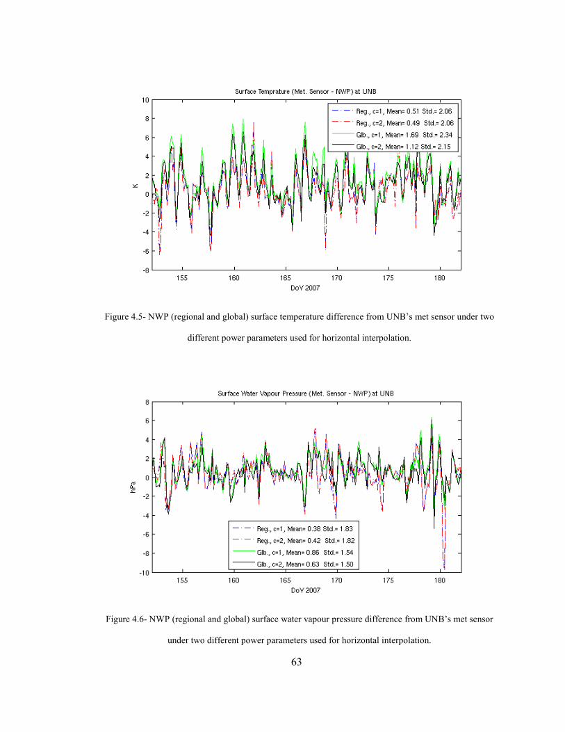
63

Figure 4.5- NWP (regional and global) surface temperature difference from UNB’s met sensor under two

different power parameters used for horizontal interpolation.

Figure 4.6- NWP (regional and global) surface water vapour pressure difference from UNB’s met sensor

under two different power parameters used for horizontal interpolation.

64

The mean difference in the values from global and regional models are significant at the

95% confidence level for both power parameters used1. Hence one may conclude that

pressure from the global model provided closer average results to the independent

measurements (met sensor) in the investigated month (see Figure 4.4). However,

temperature and water vapour pressure from the met sensor are closer to the regional

model than the global model (see Figures 4.5 and 4.6). The performance of regional vs.

global models in zenith delay results will be investigated in section 4.4.3.

After calculating the pressure, temperature, and humidity at each level, and ignoring gas

compressibility factors, one can use the following equation to derive refractivity at each

level (see also equation (2.3)):

+′+

+

−=

2321

i

wv

i

wv

iw

wv

id

wvi

diT

pk

T

pk

TR

p

TR

pPRkN iiii (4.5)

where 1k , 2k ′ and 3k are empirically determined constants introduced in equations (2.4);

dR and wR are the specific gas constants for dry air and water vapour respectively; and

iP , iT , and iwvp are pressure, temperature and water vapour pressure at level i

respectively. Integration of the terms within the second parentheses in Equation (4.5)

along the path results in the path non-hydrostatic (wet) delay while integration of the first

1 Except for mean differences of water vapour pressure from NWP models with power parameter 2 which are not significantly different at the 95% confidence level. However, one should note that water vapour pressure is not the primary measurement in the met sensor or the primary humidity parameter available from NWP models. Relative humidity from the met sensor and specific humidity from the NWP models are both converted to water vapour pressure in order to be compared.

65

part of Equation (4.5) will result in the path hydrostatic delay. If the integrations are

performed at the zenith, the resulting quantities are the ZWD and ZHD, respectively.

The neutral atmosphere contributes to the hydrostatic part of the delay up to an altitude of

about 70-80 km. Figure 4.7 shows the effect of reducing the top level of integration in the

zenith and 5 degree elevation slant delay. From the figure, one can conclude that ignoring

the atmosphere above 60 km may result in a few mm slant delay error and less than 1 mm

in the zenith delay.

The highest layers of both RAOB and NWP models end at about 20-30 km above the

Earth’s surface – below the top of the neutral atmosphere. The COSPAR International

Reference Atmosphere (CIRA) 1986 model1 has been used in the ray tracing package

from the maximum height of RAOB (or NWP model) or 20 km above the Earth’s surface

(whichever is less). The values from CIRA are shifted to match the top level values of

RAOB or NWP.

1 http://modelweb.gsfc.nasa.gov/atmos/cospar1.html

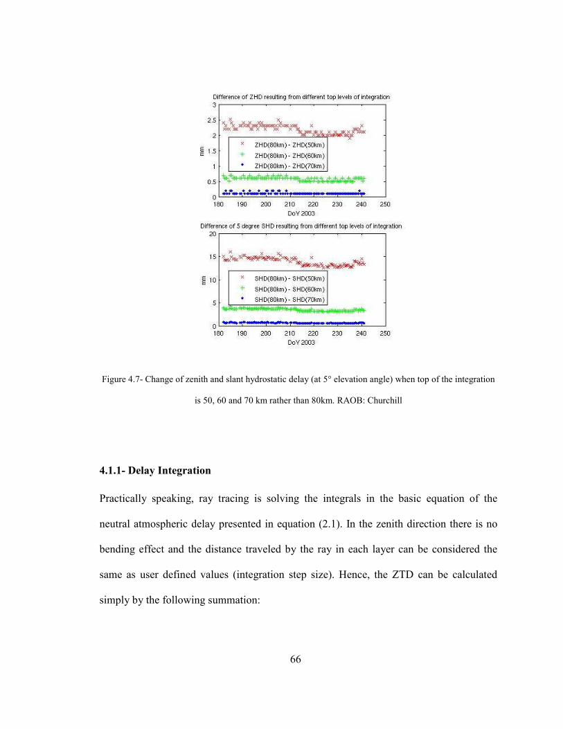
66

Figure 4.7- Change of zenith and slant hydrostatic delay (at 5° elevation angle) when top of the integration

is 50, 60 and 70 km rather than 80km. RAOB: Churchill

4.1.1- Delay Integration

Practically speaking, ray tracing is solving the integrals in the basic equation of the

neutral atmospheric delay presented in equation (2.1). In the zenith direction there is no

bending effect and the distance traveled by the ray in each layer can be considered the

same as user defined values (integration step size). Hence, the ZTD can be calculated

simply by the following summation:

67

∑=

−

⋅

+′+

+

−=

km

Surfacei

i

i

wv

i

wv

iw

wv

id

wvi

d dhT

pk

T

pk

TR

p

TR

pPRkZTD iiii

80

23216 )(10 (4.6)

where idh is the integration step size at level i and other parameters have already been

introduced in equation (4.5).

In order to trace a ray in a direction other than zenith, one requires the slant distance that

the ray travels in each layer. A simplified geometry of ray tracing in a symmetric

atmosphere is represented in Figure 4.8. Using the initial angle of the ray at the surface,

and applying Snell’s law, by assuming spherical interface layers one can calculate the

slant distance in each layer and also the angle at which the ray exits each layer (see, e.g.,

Boehm and Schuh [2003]) as follows:

)(cos)sin( 2221 iiiiii rrrs Θ−+Θ−= + (4.7)

where is is the distance of the traveled ray in layer i, ir and 1+ir are the geocentric radius

of middle points of two consecutives layers and iΘ is angle of the ray at level i with local

horizon which can be derived from the similar angle in the previous layer (e.g. in the first

layer this is the user input value) and Snell’s law as follows:

+Θ=Θ +

++ )cos(arccos 1

11 ii

i

i

in

nδ (4.8)

where in and 1+in are the refractive indexes at two consecutive layers and:

iii ψψδ −= ++ 11 (4.9)

68

where iψ and 1+iψ are geocentre angles in two consecutive levels. The angle at which

the ray exits each layer can be derived as:

111 +++ −Θ= iiie ψ (4.10)

By performing the integration from the station (surface) toward the top of the neutral

atmosphere one can finally calculate the angle at which the ray exits the neutral

atmosphere. The geometric bending effect can be derived from the following equation

and is then added to the hydrostatic delay [Boehm et al., 2006]:

[ ]∑−

=

⋅−−=1

1

)cos(k

i

ikii seesζ (4.11)

Because of bending of the ray especially at low elevation angles, the initial elevation

angle (at a user’s location) is different from the geometric elevation angle of the straight

direction from the user’s position to a GNSS satellite, for example. The amount of

bending at each layer depends on the refractivity of the layer and that of its neighbours.

Hence any error in refractivity affects this angle and accumulates in consecutive layers1.

However, one should note that the angle at which rays exit the neutral atmosphere (often

known as the vacuum elevation angle) corresponds to the geometric angle which should

be considered in GNSS analysis. Hence, an iterative approach can be employed to find

the associated refracted elevation angle corresponding to a geometric angle at the user.

1 This is probably a reason why integrating the path delay from surface toward the top of the neutral atmosphere has been common practice. For example, the software developed by J.L. Davis, T.A Herring, and A.E. Niell which was also used by Mendes [1999] also traces the path of a ray starting from the surface of the Earth travelling out of the neutral atmosphere. In this software, even though the user input is the vacuum elevation angle at the surface, an empirically determined relation is used to find the approximate corresponding refracted elevation angle (at the surface) to the user vacuum elevation angle. Three iterations are then carried out which result in three corresponding vacuum elevation angles and path delays. Finally a quadratic function is used for interpolation which results in the final path delay.

69

However for the purpose of implementing VMF1 (see Chapter 6) iteration is not required

as the corresponding vacuum elevation angle to an initial elevation angle is used in the

mapping function.

Figure 4.8- Geometry of ray tracing calculation (after Boehm and Schuh [2003, p.141]).

4.2- Data Sources for Ray Tracing

In the GNSS community, RAOB have been used for research purposes to validate

atmospheric models and mapping functions (see, e.g., Mendes, [1999]; Rocken et al.,

[2001]). RAOBs are rather sparse in time and location. More recently, NWP models have

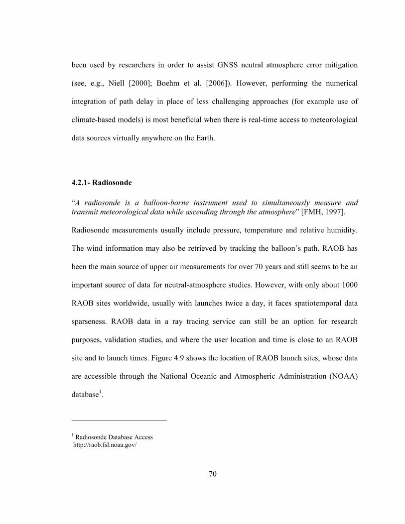
70

been used by researchers in order to assist GNSS neutral atmosphere error mitigation

(see, e.g., Niell [2000]; Boehm et al. [2006]). However, performing the numerical

integration of path delay in place of less challenging approaches (for example use of

climate-based models) is most beneficial when there is real-time access to meteorological

data sources virtually anywhere on the Earth.

4.2.1- Radiosonde

“A radiosonde is a balloon-borne instrument used to simultaneously measure and

transmit meteorological data while ascending through the atmosphere” [FMH, 1997]. Radiosonde measurements usually include pressure, temperature and relative humidity.

The wind information may also be retrieved by tracking the balloon’s path. RAOB has

been the main source of upper air measurements for over 70 years and still seems to be an

important source of data for neutral-atmosphere studies. However, with only about 1000

RAOB sites worldwide, usually with launches twice a day, it faces spatiotemporal data

sparseness. RAOB data in a ray tracing service can still be an option for research

purposes, validation studies, and where the user location and time is close to an RAOB

site and to launch times. Figure 4.9 shows the location of RAOB launch sites, whose data

are accessible through the National Oceanic and Atmospheric Administration (NOAA)

database1.

1 Radiosonde Database Access http://raob.fsl.noaa.gov/

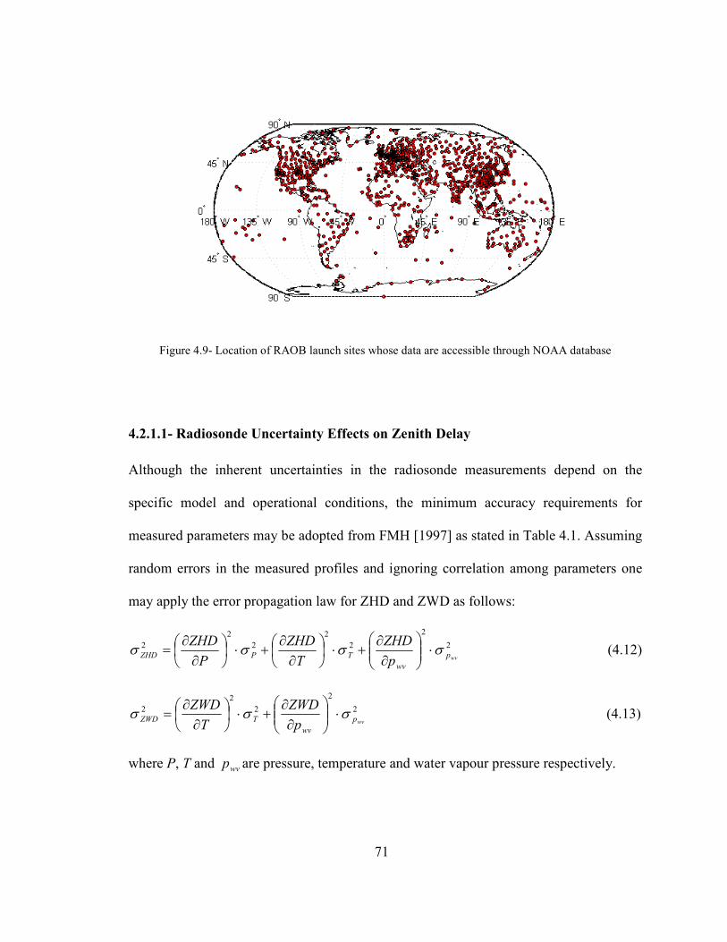
71

Figure 4.9- Location of RAOB launch sites whose data are accessible through NOAA database

4.2.1.1- Radiosonde Uncertainty Effects on Zenith Delay

Although the inherent uncertainties in the radiosonde measurements depend on the

specific model and operational conditions, the minimum accuracy requirements for

measured parameters may be adopted from FMH [1997] as stated in Table 4.1. Assuming

random errors in the measured profiles and ignoring correlation among parameters one

may apply the error propagation law for ZHD and ZWD as follows:

2

2

22

22

2

wvp

wv

TPZHDp

ZHD

T

ZHD

P

ZHDσσσσ ⋅

∂∂

+⋅

∂∂

+⋅

∂

∂= (4.12)

2

2

22

2

wvp

wv

TZWDp

ZWD

T

ZWDσσσ ⋅

∂∂

+⋅

∂

∂= (4.13)

where P, T and wvp are pressure, temperature and water vapour pressure respectively.

72

Required derivations to be used in equations (4.12) and (4.13) are as follows (see

equation (4.6)):

∑=

−

=

∂∂ n

i

i

ii

dhT

k

P

ZHD

1

1610)(

(4.14)

∑=

−

−

−−=

∂∂ n

i

i

iw

wvd

i

wvi

i

dhTR

pRk

T

pPk

T

ZHDii

12

1

2

16)(

10)(

(4.15)

∑=

−

−

′−=

∂∂ n

i

i

i

wv

i

wv

i

dhT

pk

T

pk

T

ZWDii

13

3

2

262

10)(

(4.16)

∑=

−

+

−=

∂∂ n

i

i

iw

d

iwv

dhTR

Rk

T

k

p

ZHD

i1

11610)(

(4.17)

∑=

−

+′

=∂∂ n

i

i

iiwv

dhT

k

T

k

p

ZWD

i1

232610

)( (4.18)

However one should note that iwvp is not the primary radiosonde measurable. Hence

first the propagation of errors in temperature and relative humidity on iwvp should be

calculated. Using the following conversion equation adopted from FMH [1997]:

+=

i

ii

wvt

tUp

i 97.240

502.17exp1121.6

100 (4.19)

where iU is the relative humidity and it is temperature in degrees Celsius, one can

derive:

+=

∂

∂

i

i

i

wv

t

t

U

pi

97.240

502.17exp061121.0 (4.20)

73

( )

++=

∂

∂

i

i

i

i

i

wv

t

t

t

U

t

pi

97.240

502.17exp

97.240

7752.2572

(4.21)

Using the derivations in equations (4.14) to (4.21) and assuming σ values as stated in

Table 4.1 [FMH, 1997], the effect of radiosonde uncertainties (as random errors) in

zenith delay integration can be calculated. ZHD and ZWD together with their propagated

errors calculated from RAOB at Churchill, MB, for the month of June 2007 can be seen

in Figures 4.10 and 4.11 respectively. It can be concluded that considering radiosonde

measurements’ uncertainties as random errors (and ignoring correlation among

parameters) may only have sub-millimetre level effect on both ZHD and ZWD. While the

effect is larger when the ZWD is increased, no such error variation can be seen in ZHD

(mainly because the errors are small). One should note that uncertainties in CIRA values

are assumed to follow those in Table 4.1, which might not be true. However, this should

only have minor effect on ZHD error estimates. While the result of propagated random

errors on zenith delay results seems to be promisingly small, the existence of systematic

biases in RAOB is likely. Mendes [1999] simulated a constant bias based on World

Meteorological Organization (WMO) accuracy limits on standard atmosphere profiles. It

was concluded that a 2.3 mm bias in ZHD and biases of ~2 mm to almost 3 cm in ZWD

were created. However, he stated that the accuracy of many of the current radiosonde

instruments is better than the imposed WMO limits.

74

Table 4.1- Accuracy of related radiosonde measurements that shall be considered as minimum standard

[FMH, 1997].

Variable Accuracy

Temperature 0.5ºC

Relative Humidity 5%

Pressure

2.0 hPa (P > 300 hPa)

1.5 hPa (50 hPa < P≤ 300 hPa)

1.0 hPa ( P ≤ 50 hPa)

Figure 4.10- ZHD and propagated errors (dashed line scaled on the right side) calculated from RAOB at

Churchill, MB.

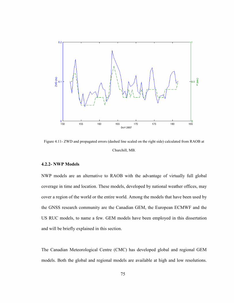
75

Figure 4.11- ZWD and propagated errors (dashed line scaled on the right side) calculated from RAOB at

Churchill, MB.

4.2.2- NWP Models

NWP models are an alternative to RAOB with the advantage of virtually full global

coverage in time and location. These models, developed by national weather offices, may

cover a region of the world or the entire world. Among the models that have been used by

the GNSS research community are the Canadian GEM, the European ECMWF and the

US RUC models, to name a few. GEM models have been employed in this dissertation

and will be briefly explained in this section.

The Canadian Meteorological Centre (CMC) has developed global and regional GEM

models. Both the global and regional models are available at high and low resolutions.

76

However, the use of a high resolution NWP model seems to be more beneficial for GNSS

applications due to proximity of grid points to user locations. Therefore high resolution

models have been employed in this work and will be briefly explained here.

Before September 20, 2007 at 12 UTC (the initialization time), the global model was

available at a resolution of 1°×1°. Subsequently, the global model became available on a

283 × 601 latitude-longitude grid (covering all the Earth except above 85°N and below

84.2°S) at a resolution of 0.6°×0.6° (which corresponds approximately to a 66 km × 66

km grid size at the equator). The model has 28 isobaric levels. As of June 3, 2008, at 12

UTC (the initialization time), the global model covers all the Earth and contains 301 ×

601 grid points. The regional GEM model contains 501 × 399 grid points with a 15 km

resolution at 60°N which is made available with 28 isobaric levels. This model covers

most of North America and adjacent waters.

In addition to surface values (values at some fixed height above ground), vertical

coverage of the three-dimensional fields for both global and regional models is provided

for the following isobaric levels (hPa): 1015, 1000, 985, 970, 950, 925, 900, 875, 850,

800, 750, 700, 650, 600, 550, 500, 450, 400, 350, 300, 275, 250, 225, 200, 175, 150, 100

and 50. Most of these levels are the same as the standard mandatory reporting levels in

RAOB. Also a few intermediate levels, especially near the surface and near the

tropopause, are added to improve vertical resolution at those levels [Pelletier, 2008].

Regional 0-48 hour forecasts and global 0-144 hour forecasts are issued twice a day,

77

based on 00 UTC and 12 UTC initialization times. All fields are available at 3-hourly

intervals1.

4.3-Online Ray Tracing Package

An online ray tracing package (hereafter referred to as Online-RT) has been developed to

provide zenith and slant delays at a user location using RAOB and NWP models. In

addition, the online service provides latest maps of ZHD, ZWD and gradients using NWP

models and provides comparisons with UNB3 and UNB3m models. The service is

currently available at http://galileo.gge.unb.ca.

Code for data access and pre-processing has been written in Linux shell script, while the

ray tracing and map-generation parts are written in MATLAB®. Although the basic ray

tracing algorithm is the same for both RAOB and NWP models, data retrieval and

manipulation are different and need to be addressed separately.

Online-RT provides automatic data access to the closest possible spatiotemporal RAOB

to the user requested location and time via NOAA’s online database. The user is

informed of the distance and azimuth of the nearest possible RAOB. Currently, NOAA’s

online database provides RAOB data from 1994 up to today. Although these data have

1 High-resolution CMC GRIB (see next page) dataset http://www.weatheroffice.gc.ca/grib/High-resolution_GRIB_e.html

78

gone through extensive quality control analysis, further quality checks have been found

to be necessary for our purpose.

Canadian NWP data is provided in gridded binary (GRIB) files. The files are based on

parameters rather than coordinates; i.e., each file includes one specific parameter of just

one specific isobaric layer for the whole set of grid points (180,901 and 199,899 points

for the global and regional models respectively). Therefore, in order to achieve a vertical

profile of meteorological parameters above a site, all GRIB files of related

meteorological parameters need to be read. The GRIB files for each initialization time

(00 and 12 UTC) are currently made available about 5 and 3 hours after the initialization

time for the global and regional models respectively. Transferring all appropriate files

from the Meteorological Service of Canada’s1 server to a local database also takes about

1-1.5 hours depending on network traffic. Therefore, in order to make sure that at any

time the Online-RT can provide results at the current time, the GRIB files for forecasts up

to 24 hours ahead are transferred. The total size of appropriate GRIB files is about 192.5

megabytes and 224.5 megabytes for global and regional models per initialization time

respectively; i.e., a total size of about 834 megabytes per day for both global and regional

models.

1 The Meteorological Service of Canada makes CMC’s GEM models output available to private sector meteorologists, academics and general public. http://www.weatheroffice.gc.ca/grib/index_e.html

79

Specific humidity is provided in the GEM models as the measure of humidity whereas

dew point temperature is accessible by RAOB. However, both measures of humidity are

converted to water vapour pressure. Dew point temperature can be converted to water

vapour pressure through knowledge of saturation vapour pressure; large numbers of

formulae are available to do this. Mendes [1999] tested four of the most widely used

formulae and found differences as large as 3 mm for ZWD. He recommended the Wexler

[1976] formula for use in saturated vapour pressure computations which is also the

formula used here. For converting specific humidity to water vapour pressure the

following approximate formula which is sufficiently accurate (see e.g. Cole [1975]) in

normal conditions1 can be used:

622.0

qPpwv

⋅≅ (4.22)

where wvp is the water vapour pressure in hPa, P is the total pressure in hPa and q is the

specific humidity in kg/kg.

A web interface to ask for a user input file (including user location and time) and email

address has been developed. After accessing the data, and carrying out data manipulation

and ray tracing, the results are sent back to the user by email. The output includes zenith

and slant (at a user-requested elevation angle) hydrostatic and wet delays, predicted

zenith values from the Saastamoinen model [Saastamoinen, 1972a, 1972b, 1973; Davis et

1 In very humid condition the given formula may over estimate the ZWD by less than 1% compared to the

accurate relation of : ( ) 622.0622.01 +⋅−

⋅=

q

qPpwv .

80

al., 1985] with surface pressure interpolated to the user height from the models or

radiosonde profiles and vacuum or unrefracted elevation angle (called VEA in Online-RT

output). A sample output for a user request of two locations using RAOB can be seen in

an example email message in Figure 4.12. As can be seen in this sample output, the

closest available RAOB launch site information, which has been used for each requested

location, is also provided.

Figure 4.12- A sample output file of the Online-RT package

Figure 4.13 shows the major steps carried out in the Online-RT package. The website

also displays near real-time global maps of zenith hydrostatic and wet delays and total,

NS and east-west (EW) gradients using the latest available Canadian global NWP model

along with maps showing the differences between the hydrostatic, wet, and total zenith

81

delays computed using the NWP model and the values computed using the UNB3 and

UNB3m climatological models.

In order to generate the latest global ZHD, ZWD, and comparison maps, almost all GRIB

files are read and first converted to a 3D array of 24×4×180,901 cells where 24 is the

number of layers, 4 represents the number of parameters (elevation, pressure,

temperature, and specific humidity), and 180,901 is the number of grid points in the

global model. One should note that there are a total of 29 layers available (including the

surface layer). The layers above 200 hPa isobaric level make less than a 0.5 mm

contribution to ZWD and hence can be ignored to speed up the map generation process.

Each of the 180,901 matrices of 24×4 cells is then used for the ZWD calculation. It has

been shown that the Saastamoinen model can provide ZHD with sub-millimetre accuracy

provided that accurate (accuracy of better than ~0.4 hPa) surface pressure is available

(see, e.g., Mendes [1999]). Therefore, the procedure for ZHD map generation uses only

the surface pressure values and the Saastamoinen model. ZHD calculation is also carried

out using mean sea level (MSL) pressure. These MSL ZHD and ZWD values at grid

points are used for generating maps of NS and EW ZHD and ZWD gradients as well as

the magnitude and azimuth of ZTD gradients.

82

Figure 4.13- Major steps in Online-RT package.

User input: Selected data.

source, bcatDn

RAOB coordimtes, NWP

I--time, elevatDn '- (Global)

[ Bi-daily access and saving ofGRIB ftles I ~. alldemail in heal database

NWP - (Regional)

Find realest s~ioWmporal Read all app10pri.te GRIB RAOB totl'e user values files

Get RAOB dat•f.,mNOAA Find 4 realest grid points to online database the user bcatDn

Zenith de loy calcul<d:Dn

using clim;4ic models at all

Qu.lityc0111>Dlwremove Mam 4 verti:al ptcf'tles for each grid locatDns

\ll1Wallled par~rs user requested bcati:wlilre

! Data. oonversDn, inc1ease Zenith de loy resolui:Dn, intetpOI<d:Dnof calcul<d:Dn using NWP p~ers totl'e user heidd, a.t a.ll grid poUts

extensionofptoftles up b:l top of the neutralatmosphe1e

I Ray tracing

! Prepare output flies (add header GeneratDnofzmith

alldothn ini>nnotion) delay, gradim and

l diffe1emed ma.ps

eV<ey 3 h>urs

Send the resulttotl'e

"'er

83

The map generation procedure is repeated every 3 hours using the NWP data providing

the shortest possible forecast time. Therefore, at any time, public users can have access to

the near real-time global maps of ZHD, ZWD, gradients, and comparisons, which are

being updated every 3 hours. The UNB climatological model values are also calculated at

the location of grid points and then differenced from the NWP-calculated values in order

to generate the difference maps. Sample maps provided by the Online-RT package at an

arbitrary epoch are provided in Appendix III. All near-real-time maps are available

publicly through the web site. A potential future use of the zenith delay map generation

service could be in the Interferometric Synthetic Aperture Radar (InSAR) application

(see, e.g., Foster et al. [2006]; Li et al. [2006]) where a high resolution weather model can

be used to reduce the atmospheric effect on InSAR interferograms.

The performance of the climatological models may be evaluated using NWP results. For

example, 3-hourly extreme differences of ZHD from global and regional NWP models

and those from UNB3 are plotted in Figures 4.14 and 4.15 respectively. These result from

monitoring of generated 3-hourly near-real-time maps over 16 months (from 1 July 2007

to 31 October 2008) such as those presented for an arbitrary epoch in Figures III.6 and

III.7 (Appendix III). The average of positive and negative extreme values can be seen in

the titles of Figures 4.14 and 4.15. Note that larger negative extreme difference values

occur in the global model. These extreme negative differences typically occur in the belt

84

around Antarctica where UNB3, which is based on a standard atmosphere1, usually

overestimates mean sea level pressure. The increased variability in negative extreme

values may indicate more variability in low pressure systems.

Figure 4.14– Extreme difference between ZHD from global high resolution Canadian NWP model and

UNB3 calculated over 16 months.

Figure 4.15– Extreme difference between ZHD from regional high resolution Canadian NWP model and

UNB3 calculated over 16 months.

1 UNB3 “uses a look up table of meteorological parameters derived from the 1966 US Standard

Atmosphere Supplements whose values vary over latitude and season” [Collins, 1999].

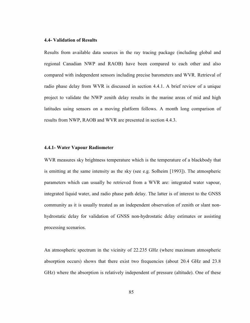
85

4.4- Validation of Results

Results from available data sources in the ray tracing package (including global and

regional Canadian NWP and RAOB) have been compared to each other and also

compared with independent sensors including precise barometers and WVR. Retrieval of

radio phase delay from WVR is discussed in section 4.4.1. A brief review of a unique

project to validate the NWP zenith delay results in the marine areas of mid and high

latitudes using sensors on a moving platform follows. A month long comparison of

results from NWP, RAOB and WVR are presented in section 4.4.3.

4.4.1- Water Vapour Radiometer

WVR measures sky brightness temperature which is the temperature of a blackbody that

is emitting at the same intensity as the sky (see e.g. Solheim [1993]). The atmospheric

parameters which can usually be retrieved from a WVR are: integrated water vapour,

integrated liquid water, and radio phase path delay. The latter is of interest to the GNSS

community as it is usually treated as an independent observation of zenith or slant non-

hydrostatic delay for validation of GNSS non-hydrostatic delay estimates or assisting

processing scenarios.

An atmospheric spectrum in the vicinity of 22.235 GHz (where maximum atmospheric

absorption occurs) shows that there exist two frequencies (about 20.4 GHz and 23.8

GHz) where the absorption is relatively independent of pressure (altitude). One of these

86

frequencies is usually used in WVRs1 to minimize the sensitivity of brightness

temperature to water vapour. Furthermore, in order to separate the effect of cloud liquid

from water vapour, another frequency (usually 31.4 GHz) is also employed in dual

frequency WVRs.

Radio phase path delay can be retrieved from opacity. Opacity may be defined as:

−

−=

ibmr

mri

TT

TT coslnτ (4.23)

where mrT is the mean radiation temperature, KT 7.2cos = is the cosmic background

temperature which results from the residual cosmic radiation from outer space that is left

from the Big Bang (see e.g. Leick [2004]), and bT is the sky brightness temperature

which is the basic WVR observable and i represents the frequency.

By using opacities at two frequencies a linear retrieval equation for slant non-hydrostatic

delay (SWD) from the opacities can be written as:

4.3128.2310 ττ ⋅+⋅+= CCCSWD (4.24)

where 0C , 1C and 2C are the retrieval coefficients. One way to derive the retrieval

coefficients is by calculating the theoretical opacities by numerical integration through

RAOB and then estimating the coefficients using a bilinear regression to opacities, liquid

and vapour arrays (see e.g. Solheim [1993]). The brightness temperatures measured by

1 In the Radiometrics WVR-1100, for example, the 23.8 GHz frequency is chosen because it is in a reserved research waveband where no radio transmission is allowed [Solheim, 1993].

87

WVR are used to calculate opacities at each of the two frequencies (see equation (4.23)).

Using the retrieval coefficients and opacities one can calculate the SWD from equation

(4.24).

From the retrieval approach briefly discussed above, one can conclude that WVR phase

delay results are dependent on RAOB data at a particular location or locations. In

practice, long term RAOB data from the same climatological region in which the WVR is

operating are used for deriving the coefficients. While among the WVR retrievable

parameters, phase delay is less dependent on the location of RAOB (and change of the

retrieval coefficients), this dependence has been investigated during a field experiment

carried out as part of this dissertation research work.

4.4.2- Precise Barometer and WVR on a Moving Platform for NWP Validation

There are very few reports on the performance of a WVR on a moving platform.

Researchers at the University of Miami set up a WVR on the Royal Caribbean Cruise

Line ship Explorer of the Seas [Minnett, 2004]. The experiment was also used to compare

WVR and GPS results [Rocken et. al., 2005].

During the 2005 Canadian research icebreaker Canadian Coast Guard Ship (CCGS)

Amundsen’s mission in the Canadian Arctic an experiment was carried out by the author

to investigate the performance of the Canadian regional NWP model. As a part of this

experiment our Radiometrics WVR-1100 was set up on the ship’s deck (see Figure 4.16)

88

and was programmed to record zenith as well as some specific slant measurements. A

precise barometer1 was also set up on the ship and provided a continuous record of the

surface atmospheric pressure.

Figure 4.16- WVR onboard CCGS Amundsen

As mentioned in section 4.4.1 non-hydrostatic delays from a WVR are actually obtained

from the observed brightness temperature and the estimated retrieval coefficients. These

coefficients can be estimated from long term radiosonde measurements in the same

climatological region as that in which the WVR operates. A retrieval program provided

by Radiometrics Corporation has been used in this experiment. In order to investigate

how different coefficients might affect the final WVR ZWD, three scenarios have been

considered:

1 A Honeywell Precision Barometer with accuracy of better than ±0.4 hPa (from -40 to 80°C) [Honeywell, 2005] was validated using the Suominet station barometer at UNB before installation on board the CCGS Amundsen.

89

1. Default retrieval coefficients derived from a radiosonde near UNB at a latitude of

~46° N.

2. Retrieval coefficients from the nearest radiosonde using the 3 months of data that

span the date of measurement. Different sets of coefficients (from 6 years of data

from 10 nearby radiosondes) were derived and used based on the proximity of the

ship to a particular radiosonde site during the expedition (see Figure 4.17).

3. Same as 2 but using the entire 6 year radiosonde data sets.

Figure 4.17- CCGS Amundsen expedition track on her 2005 mission and location of radiosonde sites used

for retrieval coefficients.

90

The difference between the results from scenarios 2 and 3 was found to be negligible

(about 0.04 cm in ZWD on average). Figure 4.18 shows the measured ZWD during the

expedition as well as absolute and relative differences of ZWD resulting from scenarios 1

and 2. As can be seen in Figure 4.18c the change of retrieval coefficients affect the

resulted WVR ZWD by less than 4% in most cases. The result from scenario 2 has been

selected as the final WVR ZWD in this study.

Figure 4.18– a) ZWD during the expedition. b) Absolute difference between ZWD from scenarios 1 and 2.

c) Relative difference between scenarios 1 and 2.

91

In order to carry out the tip curve calibration1 of the WVR noise diode injection

temperatures, the WVR needs to be accurately levelled which was not possible on board

the vessel. Therefore the calibration values obtained before the expedition were used.

Figures 4.19 and 4.20 show a comparison between NWP and barometer pressure

measurements corrected to the GPS antenna height during parts of the expedition

(Canadian Arctic, Sub-Arctic and mid-latitudes). The RMS of the differences is less than

1 hPa for the compared data series. Assuming no error in the Saastamoinen model,

height and latitude, an uncertainty of less than 1hPa in surface pressure measurement will

result in less than 2.3 mm error in the ZHD. The figures also include the predicted

pressure from UNB3, a climate based neutral atmosphere model. The models and

measurements are in closer agreement in Figure 4.20 (mid-latitudes) than in Figure 4.19

(high latitude). However, in the case of NWP, this may be partly due to the fact that only

initialization (00 and 12 UTC) data were used in Figure 4.20.

1 Tip curve calibration is a technique to calibrate instrument gain and accurate estimate of brightness temperature without any a priori knowledge of either. In this technique several sky observations are made at different elevation angles which provide observations through different air masses. The assumptions made are that the atmosphere is horizontally homogeneous and opacity is a linear function of air mass (hence the linear regression to line through the opacities must pass through the origin at zero air mass and zero opacity). The regression coefficient of the linear fit to opacities is an indicator of the calibration acceptance. One may refer to e.g. Solheim [1993] or Leick [2004] for more details on this technique.

92

Figure 4.19– Measured and NWP Pressure values in the Canadian Arctic.

Figure 4.20– Measured and NWP Pressure values in the Canadian-Sub Arctic and mid-latitudes.

93

Figures 4.21 and 4.22 show the WVR ZWD results as compared with those calculated

from the NWP. The RMS of the difference between smoothed WVR (using a MATLAB

built-in function of 50th order finite impulse response low pass filter which in this case is

roughly close to a 1-hour moving average filter) and NWP are at the cm level. The

figures also include the ZWD from the UNB3m model. As expected, the uncertainty in

retrieving the wet delays in this study is about 1 order of magnitude larger than those of

the hydrostatic delays. Liquid water or ice on a WVR antenna degrades the accuracy of

brightness temperature measurements [Ware et al., 2004]. Therefore recorded data with

liquid water values above 0.05 cm were removed before comparison. However, the

largest difference usually occurs during the time of rapid change in wet delays at peak

values. Apart from systematic and random errors that might exist in both the WVR and

NWP, the larger differences at peak values might be due to local effects on the WVR

measurements onboard and local scale weather phenomena which might not be detectable

by the NWP with a 15 km resolution.

The values compared in Figures 4.21 and 4.22 are zenith measurements and not the slant–

mapped-to-zenith values. This is of concern on a moving vessel as the true elevation

angle of the WVR’s line of sight may change due to the roll and pitch of the vessel.

However, a maximum 7 degree roll or pitch which was the case during a few periods of

the expedition does not have a significant effect on the WVR zenith measurements.

Calculating the NMF for an 83 degree elevation angle shows that a 7 degree roll or pitch

can cause about 0.75% error on the WVR ZWD results and is, therefore, insignificant.

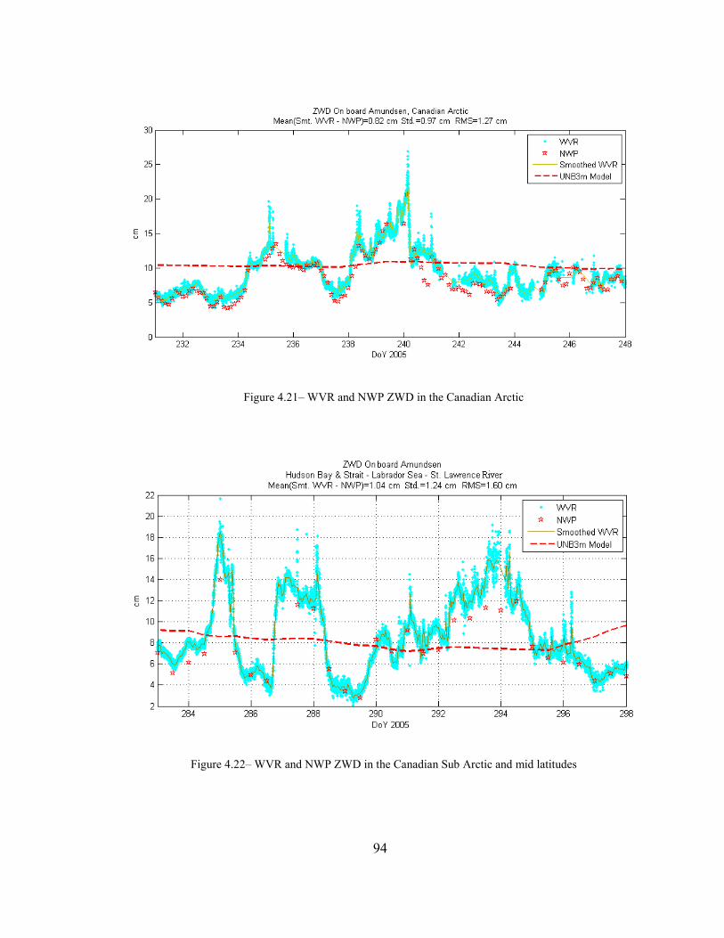
94

Figure 4.21– WVR and NWP ZWD in the Canadian Arctic

Figure 4.22– WVR and NWP ZWD in the Canadian Sub Arctic and mid latitudes

95

4.4.3- Validation at RAOB Locations and WVR at UNB

In order to compare the results of ray tracing from different available data sources in

Online-RT, the package was employed to compute the results for zenith delays at over 66

radiosonde sites (see Appendix I) in the area covered by both regional and global models.

The comparison took place using data over the month of June 2007. It should be noted

that the compared data sets are highly correlated because the radiosonde data are

assimilated into both models. However, currently there is a major difference in data

assimilation schemes used by the two models1. Furthermore, data sources available for

the two models are different due to the difference in time at which the models are run

[Verner, 2008].

The relevant statistics resulting from a comparison of the global and regional models at

the location of radiosonde sites are provided in Table 4.2. The resulting ZHD values from

the two models are in good agreement. The RMS of the ZHD difference from the global

and regional models over the compared month and locations is 1.7 mm. The RMS

increases to 11.3 mm for ZWD.

1 Currently, the regional model uses a three-dimensional variational data assimilation (3D-Var) system while the global model uses a four-dimensional variational data assimilation (4D-Var) system. One major difference between these two data assimilation approaches is that in the 4D-Var, observations are actually assimilated at their valid time of observation, while in 3D-Var observations received in a period of time are all used as if they were taken at the main synoptic time [Verner, 2008]. Hence the global model currently uses a more realistic data assimilation approach. This might be a reason why one may not simply expect more accurate zenith delay results from the regional model because of higher resolution.

96

Table 4.2- Difference between global and regional NWP model results

Global-Regional

Mean diff. (mm)

Std. (mm) Abs. max diff. (mm)

No. of data points

ZHD 0.6 1.6 9.5 16080 ZWD -0.4 11.3 76.5 16080

In Figure 4.23, one can see the histograms of the ZHD and ZWD differences between the

values from the global and regional models and those from the radiosondes. Also in

Table 4.3, the statistics of these comparisons are provided. The regional model has

provided results slightly closer to the RAOB values. This is partly due to the higher

resolution of the model and hence less uncertainty caused by our spatial interpolation

techniques between grids. The disagreement in ZWD is about five times larger than ZHD

(note the different horizontal scales in Figure 4.23). This is mainly due to the larger

uncertainty in observation and prediction of humidity in all data sources. Furthermore, as

mentioned before, linear interpolation of humidity and temperature (which might not

always be valid) can be another source of error. However, all of the interpolation

techniques may cause large errors under unusual local weather conditions. This is of

more concern when there is a large difference between the user height and the surface

level of the data source. This can also result in outlier values in some cases. The outlier

values in the investigated data sets of regional and global NWP models compared to

RAOB have occurred at the same times and locations. This can be due to local weather

anomalies affecting a radiosonde or data quality issues.

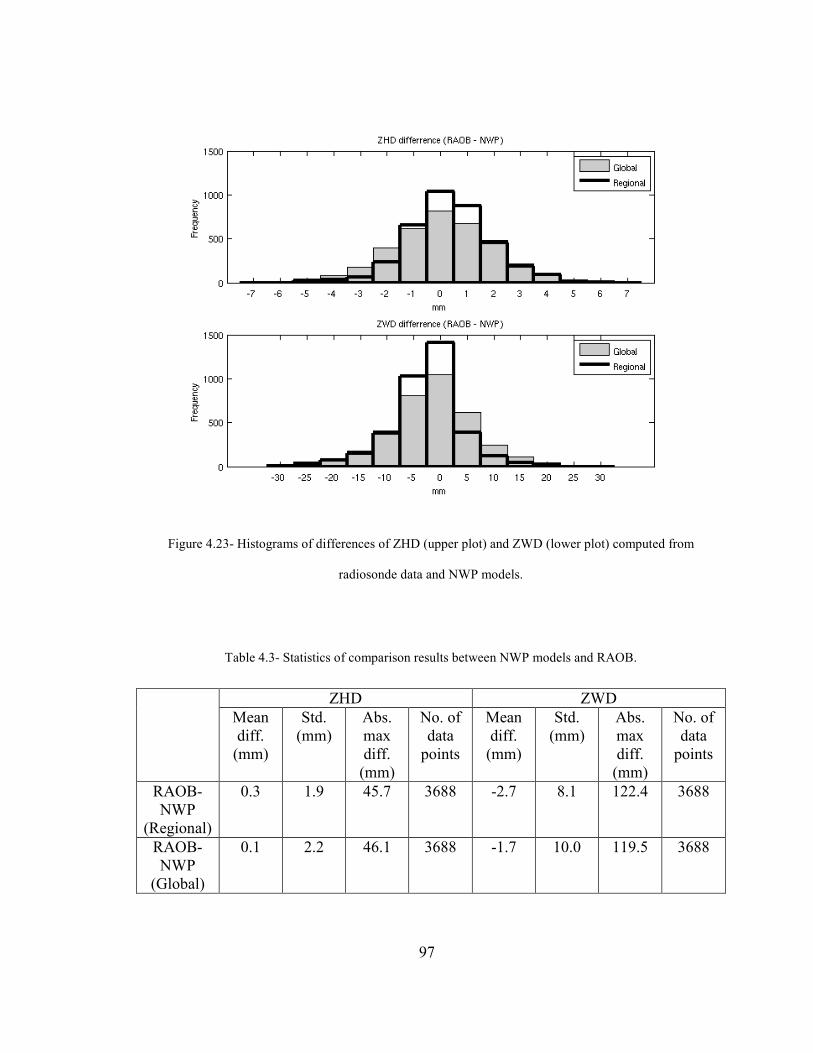
97

Figure 4.23- Histograms of differences of ZHD (upper plot) and ZWD (lower plot) computed from

radiosonde data and NWP models.

Table 4.3- Statistics of comparison results between NWP models and RAOB.

ZHD ZWD Mean diff. (mm)

Std. (mm)

Abs. max diff. (mm)

No. of data points

Mean diff. (mm)

Std. (mm)

Abs. max diff. (mm)

No. of data points

RAOB-NWP

(Regional)

0.3 1.9 45.7 3688 -2.7 8.1 122.4 3688

RAOB-NWP (Global)

0.1 2.2 46.1 3688 -1.7 10.0 119.5 3688

98

In order to compare the NWP models’ zenith delay results with independent approaches,

WVR measurements and surface pressures from UNB’s Suominet station were employed

for ZWD and ZHD estimation respectively. The UNB Radiometrics WVR-1100 operates

about 5 m (horizontally) from the UNB Suominet station. Brightness temperatures are

measured by the WVR at different azimuths and elevation angles. In this study, slant wet

delays above a 10 degree elevation angle at the WVR were converted to ZWD using the

NMF. The resulting WVR ZWD data set was then averaged over 3-hour step sizes for

comparison with NWP ZWD results. The Saastamoinen model together with pressure

measurements from the Suominet station were used to estimate ZHD.

In Figure 4.24, ZWD at the location of the WVR resulting from the NWP models using

the ray tracing package is compared to that from the WVR. The relevant statistics are

provided in Table 4.4. We note that errors in WVR estimates of ZWD can reach 16-20

mm for very humid conditions [Coster et al., 1997]. Furthermore, we note that the larger

difference of NWP results with respect to the WVR compared to those with respect to

radiosondes (Table 4.3) is partly due to the fact that radiosonde launch times are limited

to initialization times (00 and 12 UTC) and hence the radiosonde-NWP comparison was

only based on NWP initialization times (and not the 3-hour forecast). The difference is

also partly due to the fact that WVR-derived ZWD is responding to very local conditions

in different azimuth and elevation angles whereas the NWP-derived results represent a

weighted average over the nearest grid points. Figure 4.25 shows the difference between

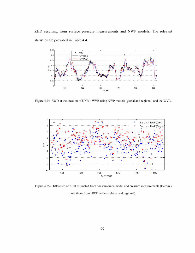
99

ZHD resulting from surface pressure measurements and NWP models. The relevant

statistics are provided in Table 4.4.

Figure 4.24- ZWD at the location of UNB’s WVR using NWP models (global and regional) and the WVR.

Figure 4.25- Difference of ZHD estimated from Saastamoinen model and pressure measurements (Barom.)

and those from NWP models (global and regional).

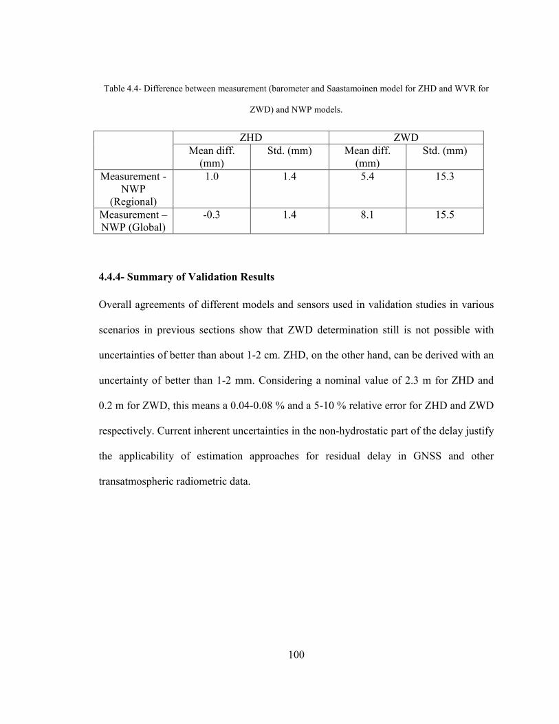
100

Table 4.4- Difference between measurement (barometer and Saastamoinen model for ZHD and WVR for

ZWD) and NWP models.

ZHD ZWD Mean diff. (mm)

Std. (mm) Mean diff. (mm)

Std. (mm)

Measurement -NWP

(Regional)

1.0 1.4 5.4 15.3

Measurement –NWP (Global)

-0.3 1.4 8.1 15.5

4.4.4- Summary of Validation Results

Overall agreements of different models and sensors used in validation studies in various

scenarios in previous sections show that ZWD determination still is not possible with

uncertainties of better than about 1-2 cm. ZHD, on the other hand, can be derived with an

uncertainty of better than 1-2 mm. Considering a nominal value of 2.3 m for ZHD and

0.2 m for ZWD, this means a 0.04-0.08 % and a 5-10 % relative error for ZHD and ZWD

respectively. Current inherent uncertainties in the non-hydrostatic part of the delay justify

the applicability of estimation approaches for residual delay in GNSS and other

transatmospheric radiometric data.

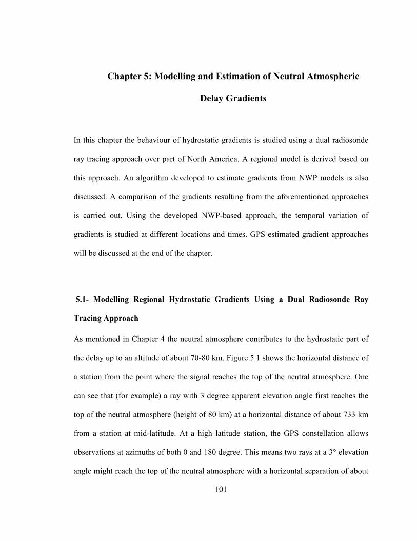
101

5. Chapter 5: Modelling and Estimation of Neutral Atmospheric

Delay Gradients

In this chapter the behaviour of hydrostatic gradients is studied using a dual radiosonde

ray tracing approach over part of North America. A regional model is derived based on

this approach. An algorithm developed to estimate gradients from NWP models is also

discussed. A comparison of the gradients resulting from the aforementioned approaches

is carried out. Using the developed NWP-based approach, the temporal variation of

gradients is studied at different locations and times. GPS-estimated gradient approaches

will be discussed at the end of the chapter.

5.1- Modelling Regional Hydrostatic Gradients Using a Dual Radiosonde Ray

Tracing Approach

As mentioned in Chapter 4 the neutral atmosphere contributes to the hydrostatic part of

the delay up to an altitude of about 70-80 km. Figure 5.1 shows the horizontal distance of

a station from the point where the signal reaches the top of the neutral atmosphere. One

can see that (for example) a ray with 3 degree apparent elevation angle first reaches the

top of the neutral atmosphere (height of 80 km) at a horizontal distance of about 733 km

from a station at mid-latitude. At a high latitude station, the GPS constellation allows

observations at azimuths of both 0 and 180 degree. This means two rays at a 3° elevation

angle might reach the top of the neutral atmosphere with a horizontal separation of about

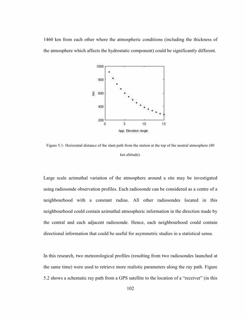
102

1460 km from each other where the atmospheric conditions (including the thickness of

the atmosphere which affects the hydrostatic component) could be significantly different.

Figure 5.1- Horizontal distance of the slant path from the station at the top of the neutral atmosphere (80

km altitude).

Large scale azimuthal variation of the atmosphere around a site may be investigated

using radiosonde observation profiles. Each radiosonde can be considered as a centre of a

neighbourhood with a constant radius. All other radiosondes located in this

neighbourhood could contain azimuthal atmospheric information in the direction made by

the central and each adjacent radiosonde. Hence, each neighbourhood could contain

directional information that could be useful for asymmetric studies in a statistical sense.

In this research, two meteorological profiles (resulting from two radiosondes launched at

the same time) were used to retrieve more realistic parameters along the ray path. Figure

5.2 shows a schematic ray path from a GPS satellite to the location of a “receiver” (in this

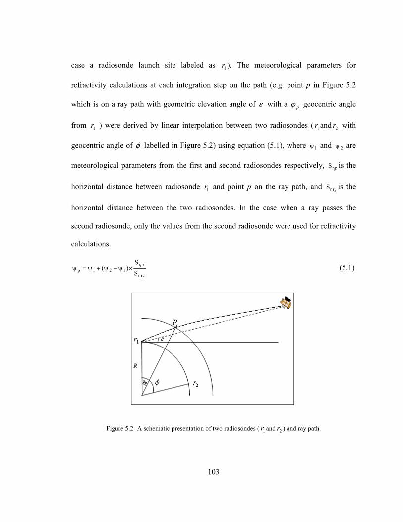
103

case a radiosonde launch site labeled as 1r ). The meteorological parameters for

refractivity calculations at each integration step on the path (e.g. point p in Figure 5.2

which is on a ray path with geometric elevation angle of ε with a pϕ geocentric angle

from 1r ) were derived by linear interpolation between two radiosondes ( 1r and 2r with

geocentric angle of φ labelled in Figure 5.2) using equation (5.1), where 1ψ and 2ψ are

meteorological parameters from the first and second radiosondes respectively, pr1S is the

horizontal distance between radiosonde 1r and point p on the ray path, and 21rrS is the

horizontal distance between the two radiosondes. In the case when a ray passes the

second radiosonde, only the values from the second radiosonde were used for refractivity

calculations.

21

1

rr

pr121p S

S)( ×ψ−ψ+ψ=ψ (5.1)

Figure 5.2- A schematic presentation of two radiosondes ( 1r and 2r ) and ray path.

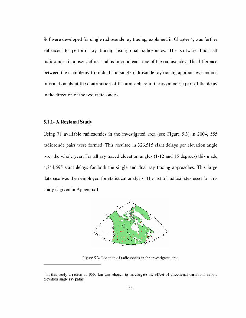
104

Software developed for single radiosonde ray tracing, explained in Chapter 4, was further

enhanced to perform ray tracing using dual radiosondes. The software finds all

radiosondes in a user-defined radius1 around each one of the radiosondes. The difference

between the slant delay from dual and single radiosonde ray tracing approaches contains

information about the contribution of the atmosphere in the asymmetric part of the delay

in the direction of the two radiosondes.

5.1.1- A Regional Study

Using 71 available radiosondes in the investigated area (see Figure 5.3) in 2004, 555

radiosonde pairs were formed. This resulted in 326,515 slant delays per elevation angle

over the whole year. For all ray traced elevation angles (1-12 and 15 degrees) this made

4,244,695 slant delays for both the single and dual ray tracing approaches. This large

database was then employed for statistical analysis. The list of radiosondes used for this

study is given in Appendix I.

Figure 5.3- Location of radiosondes in the investigated area

1 In this study a radius of 1000 km was chosen to investigate the effect of directional variations in low elevation angle ray paths.

105

Figure 5.4 shows the average difference between dual and single radiosonde ray tracing

at a 3 degree apparent elevation angle for the slant hydrostatic delay. The error bars are

the standard deviation over the whole year of 2004. It can be seen that all possible pairs

of radiosondes provide almost a full range of azimuths. The black curve in the figure (in

the polar plots as well) is the result of a nonlinear least-squares fit of a trigonometric

function which will be discussed in the next section.

Figure 5.4- a) Average differences of dual – single ray tracing of slant hydrostatic delay (3° elevation

angle) vs. azimuth (red dots with error bars) and fitted model (black curve). b) Same as above but in polar

plot and without error bars. Note that the dashed concentric circles inside the polar form are representing -

3, 0 and +3 cm from inside toward outside respectively. c): Same as above but for absolute differences.

106

Figure 5.4b shows a systematic decrease of SHD towards north (azimuths of 0°) and an

increase towards south. Figure 5.4c shows values around zero in the EW direction. The

variation of yearly averaged values vs. latitude and azimuth can be seen in the 3D plot in

Figure 5.5. A clear systematic NS average gradient can be seen in Figures 5.4 and 5.5.

Figure 5.5- Yearly average differences of dual – single ray tracing of slant hydrostatic delay (3° elevation

angle) vs. azimuth and latitude.

The results for slant wet delay (not shown here) do not show such a clear trend. This

might be partly due to the limitation of the current approach in which the closest

107

radiosonde pairs in the investigated area are about 115 km from each other. Hence the

current semi-3D ray tracing approach cannot detect the usually small scale variation in

the wet delay behaviour. However, even with this approach, a slight NS wet gradient can

be detected in some months. The NS gradient for both hydrostatic and wet components of

the delay is expected. The former is mainly the result of the decreasing thickness of the

atmosphere towards the pole and the later is due to the general decrease of humidity with

increasing latitude in the investigated area. One can see as an example the thickness map

of the atmosphere between the 500 and 1000 hPa isobaric levels and a ZWD map over

Canada and northern US for an arbitrary epoch in Figures 5.6 and 5.7 respectively. The

values used to produce the maps were calculated using the Canadian high resolution

regional NWP model. It should be noted that the ZWD is also affected by surface height

as seen in Figure 5.7 (e.g. the Rockies have low values).

108

Figure 5.6- Thickness of the atmosphere between 500 and 1000 hPa at 21 UTC 05-Sep-2007 over area

covered by regional Canadian NWP model.

Figure 5.7- ZWD at 21 UTC 05-Sep-2007 over area covered by regional Canadian NWP model.

109

5.1.2- Modelling Azimuth-dependent Hydrostatic Slant Delays

Using the created database, an effort was made to model the nominal hydrostatic

gradients in the investigated area. In order to study the monthly variation of the

hydrostatic gradients the database is divided into 12 monthly periods. For each of the 555

radiosonde pairs, mean and variance of the difference between slant delays (dual – single

RAOB ray tracing) over each month can be written as:

( )( )( )

( )( )( )

−−

−=

−

=

−−

−=

−

=

∑∑

∑∑

=

=

=

=

12

12

1

1

1

2

12,,,,12

212

12

1,,,,

12

1

2

1,,,,1

21

1

1,,,,

1

1

1

1

1

n

j

j

c

j

azci

n

j

j

c

j

azci

n

j

j

c

j

azci

n

j

j

c

j

azci

mddnn

dd

m

mddnn

dd

m

εε

εε

εε

εε

σ

σ

MM (5.2)

where 121 ,, nn K are the number of simultaneous RAOB at the central RAOB c and

directional RAOB i (which may vary for each pair of radiosondes) in months 1 to 12

respectively; j

azcid ε,,, is slant delay (with elevation angleε ) calculated using RAOBs i and

c which are at an azimuth az at observation epoch j, and j

cd ε, is the slant delay (with

elevation angleε ) from single central RAOB c.

The following function is fitted to the monthly averaged values ( 121 , mm K ) for each ray

traced elevation angle using a non-linear weighted least-squares approach:

)sin()cos(. azgazgd EN += (5.3)

110

Hence we can write:

[ ] 12,,1,,

)sin()cos(

)sin()cos(

1

11

KKMM ==

⋅

= immd

g

g

azaz

azaz

dT

ikii

iE

N

ikk

i (5.4)

where k is the number of radiosonde pairs (in this case 555) and Ng and Eg are being

estimated. The weights are calculated using the variance of monthly values as follow:

12,,1,12

K== iwi

i σ (5.5)

The estimated parameters are plotted in Figure 5.8. The NS elevation-angle-dependent

gradients become significant at low elevation angles. There is also a yearly average

change up to about 4 cm (at a 3 degree elevation angle) in this component with the largest

values in the winter months. As expected, the EW component has a smaller average value

and it is hard to interpret (lower plot in Figure 5.8).

111

Figure 5.8- The estimated elevation-angle-dependent hydrostatic asymmetry at low elevation angles for

each month and the whole year of 2004.

The following models are fitted to the results of 13 elevation angles (1-12 and 15

degrees) per each month:

)exp(ˆ ε⋅⋅= NNN bag (5.6)

)exp(ˆ ε⋅⋅= EEE bag (5.7)

where Ng and Eg are the elevation-angle-dependent gradients, Na , Nb , Ea and Eb are

given in Table 5.1 and ε is the elevation angle in degrees.

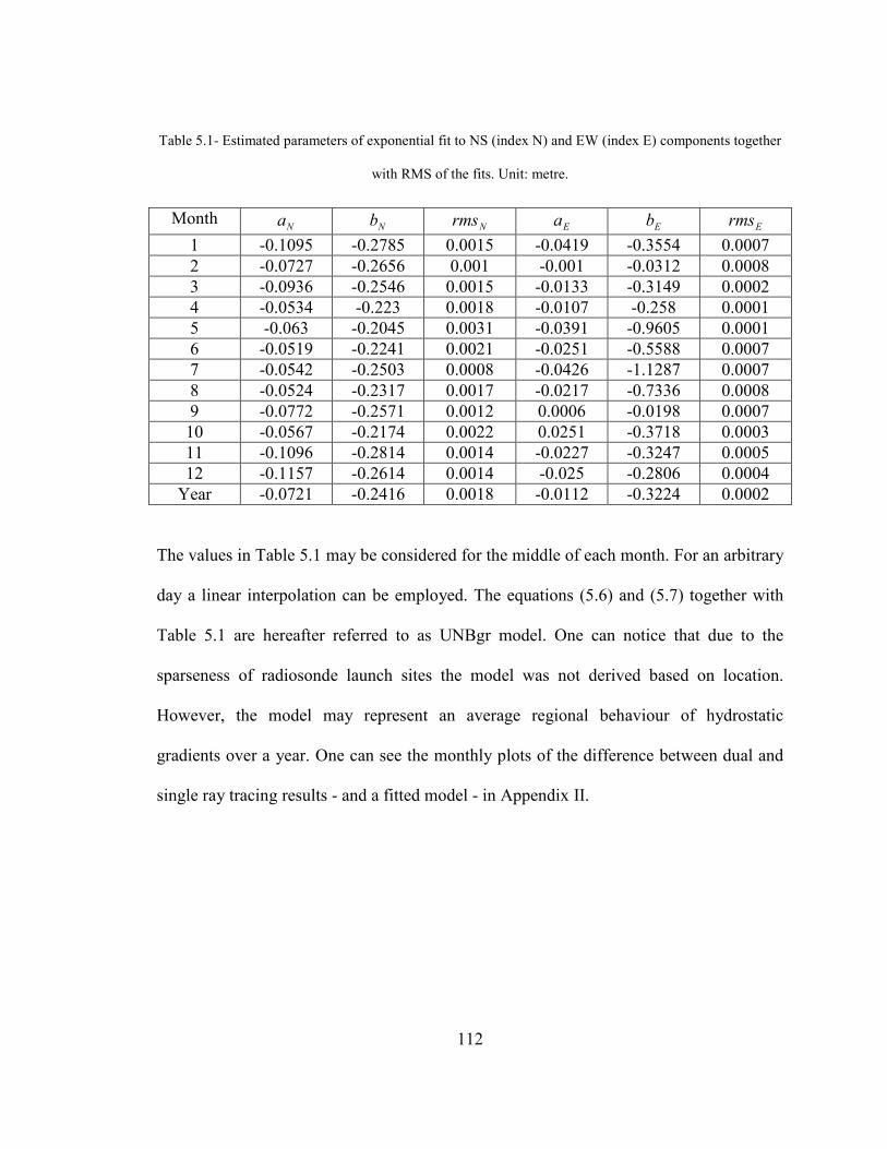
112

Table 5.1- Estimated parameters of exponential fit to NS (index N) and EW (index E) components together

with RMS of the fits. Unit: metre.

Month Na Nb Nrms Ea Eb Erms

1 -0.1095 -0.2785 0.0015 -0.0419 -0.3554 0.0007 2 -0.0727 -0.2656 0.001 -0.001 -0.0312 0.0008 3 -0.0936 -0.2546 0.0015 -0.0133 -0.3149 0.0002 4 -0.0534 -0.223 0.0018 -0.0107 -0.258 0.0001 5 -0.063 -0.2045 0.0031 -0.0391 -0.9605 0.0001 6 -0.0519 -0.2241 0.0021 -0.0251 -0.5588 0.0007 7 -0.0542 -0.2503 0.0008 -0.0426 -1.1287 0.0007 8 -0.0524 -0.2317 0.0017 -0.0217 -0.7336 0.0008 9 -0.0772 -0.2571 0.0012 0.0006 -0.0198 0.0007 10 -0.0567 -0.2174 0.0022 0.0251 -0.3718 0.0003 11 -0.1096 -0.2814 0.0014 -0.0227 -0.3247 0.0005 12 -0.1157 -0.2614 0.0014 -0.025 -0.2806 0.0004 Year -0.0721 -0.2416 0.0018 -0.0112 -0.3224 0.0002

The values in Table 5.1 may be considered for the middle of each month. For an arbitrary

day a linear interpolation can be employed. The equations (5.6) and (5.7) together with

Table 5.1 are hereafter referred to as UNBgr model. One can notice that due to the

sparseness of radiosonde launch sites the model was not derived based on location.

However, the model may represent an average regional behaviour of hydrostatic

gradients over a year. One can see the monthly plots of the difference between dual and

single ray tracing results - and a fitted model - in Appendix II.

113

5.2- Estimation of Horizontal Delay Gradients from NWP Models

With the assumption of a linear variation of refractivity with horizontal distance, the

delay gradient contributions to the slant delay (often just referred to as delay gradients or

horizontal gradients) can be defined as follows [Davis et al., 1993]:

∫ ∇= − H

Surfewew dhNhG 610 (5.8a)

∫ ∇= − H

Surfnsns dhNhG 610 (5.8b)

where ewN∇ and nsN∇ are the gradients of refractivity in the EW and NS directions

along the vertical profile respectively, h is the height along the vertical profile and H is

the altitude of the top of the neutral atmosphere (hydrostatic or non-hydrostatic). The

gradients in equations (5.8) have the same units as the path delay while the gradient of

the zenith delay has units of path delay per unit of distance. The gradients defined in

equations (5.8) are equivalent to those that can be achieved by a single GPS antenna

parameter estimation process. The gradient of the zenith delay, on the other hand, may be

estimated using GPS zenith delay estimates at more than one location. Both of the

aforementioned types of gradients can be derived from NWP models. The latest global

maps of the zenith delay gradients are currently provided every 3 hours on UNB’s

Online-RT website (see section 4.3 and appendix III for an example of zenith delay

gradient maps). However, in order to correct slant delays by NWP gradients, the delay

gradients need to be estimated at the location of the GPS antenna. An algorithm has been

developed that enables the calculation of delay gradients using the NWP models at the

user location.

114

Estimation of horizontal gradients defined in equations (5.8) requires a numerical

gradient calculation of the refractivity field. Horizontal refractivity may be assumed in a

two dimensional field where refractivity (N) is a function of easting (e) and northing (n)

i.e.:

),( nefN = (5.9)

Hence the gradient of refractivity in a flat earth approximation can be written as:

jn

fi

e

f

n

f

e

fN ˆˆ,

∂∂

+∂∂

=

∂∂

∂∂

=∇ (5.10)

where i and j are the unit vectors in easting and northing directions respectively. The

two terms on the right hand side of equation (5.10) define the EW and NS refractivity

gradients as follows:

ie

fN e

ˆ∂∂

=∇ (5.11a)

jn

fN n

ˆ∂∂

=∇ (5.11b)

Equations (5.11a) and (5.11b) are the change of refractivity per unit of distance in the

EW and NS directions respectively.

The refractivity gradient (weighted by height) along a profile at a grid point may be

numerically integrated in the NS and EW directions as follows:

∑= −+

−+

⋅

−=∇

n

k

k

ii

kikikh

ns dhS

NNhN

1 1,1

,1,1 )( (5.12a)

115

∑= −+

−+

⋅

−=∇

n

k

k

jj

kjkjkh

ew dhS

NNhN

1 1,1

,1,1 )( (5.12b)

where:

- kh is the height of level k,

- kiN ,1+ and kiN ,1− are refractivities at one grid point to the north and one grid point

to the south respectively both at level k,

- kjN ,1+ and kjN ,1− are refractivities at one grid point to the east and one grid point

to the west respectively both at level k,

- 1,1 −+ iiS and 1,1 −+ jjS are the distance between those grid points in the NS and EW

directions, and

- kdh is the integration step size at level k (see Figure 5.9 for a representation).

Equations (5.12) may then be used for estimation of horizontal gradients at each of the 4

nearest grid points to the user location, i.e.:

4,,110 ,6K=∇⋅= − mNG mh

ns

m

ns (5.13a)

4,,110 ,6K=∇⋅= − mNG mh

ew

m

ew (5.13b)

The horizontal gradient at the user location can finally be interpolated using the same

approach used for zenith delay mentioned in Chapter 4, i.e.:

∑=

⋅=4

1m

m

nsPm

P

ns GwG (5.14a)

∑=

⋅=4

1m

m

ewPm

P

ew GwG (5.14b)

116

where weights can be calculated as:

4,,14

1

K==

∑=

−

−

mw

m

c

Pm

c

PmPm

ρ

ρ (5.15)

where Pmρ is the distance between user point P and each of the 4 grid points (see Figure

5.9), and c is the power parameter. A value of 1 is used here for the power parameter.

Figure 5.9- A schematic representation of horizontal gradient calculations from NWP grids.

117

5.3- Comparison of Different Gradient Retrieval Approaches

The dual radiosonde ray tracing approach explained in section 5.1 was applied in the

same region (see Figure 5.3) but using data over the month of August 2007. This is

chosen as a benchmark for comparing:

- NWP-based gradient retrieval,

- the UNBgr model,

- and the commonly used gradient mapping functions including:

o Davis,

o Chen and Herring (CH) and

o derivative of non-hydrostatic VMF1 (VMFW1) with respect to zenith angle

(see Chapter 3).

Gradient calculation using NWP was performed at locations collocated with the

investigated radiosonde launch sites, including the central site shown in Figure 5.10 (The

Pas, MB). The comparison between Davis, CH and the derivative of VMFW1 (all using

NWP-retrieved hydrostatic horizontal delay gradients), the dual ray tracing approach and

UNBgr are plotted in Figure 5.11 for each azimuth made between radiosonde pairs at a 5

degree elevation angle over the month of August 2007.

118

Figure 5.10- Locations of radiosonde sites used for validation of gradient retrieval approaches.

In Figure 5.12, a comparison with the dual RAOB ray tracing approach in each of the

directions, then summarized as error bar plots (mean and standard deviation), is shown.

One can see that in this investigated case the CH mapping function and derivative of

VMFW1, followed by UNBgr, provided closer results to the dual RAOB ray tracing

approach than the Davis mapping function. One should note that in CH, Davis and the

derivative of VMFW1, NWP horizontal delay gradients were used while the elevation-

angle-dependent part is included in UNBgr.

119

Figure 5.11- Comparison between Davis, CH and the derivative of VMFW1 (all using NWP-retrieved

hydrostatic horizontal delay gradients), the dual RAOB ray tracing approach and the UNBgr model at

central station YQD (The Pas, MB). Elevation angle: 5°.

Similar results were derived at other radiosonde pairs in the investigated region. One can

see in Figure 5.11 that there is a generally good agreement between the dual radiosonde

ray tracing approach and NWP-retrieved gradients mapped with gradient mapping

functions. Despite the fact that UNBgr is based on an average fit to monthly data (and

hence is not expected to represent daily variations), statistically speaking, it has provided

120

closer results to dual ray tracing than the Davis mapping function (which benefited from

real-time NWP horizontal gradients) over the investigated month as seen in Figure 5.12.

Figure 5.12- Mean and standard deviation of differences from dual RAOB ray tracing for each direction

shown in Figure 5.10 with 5 degree elevation angle. a) Davis. b) CH. c) UNBgr. d) Derivative of VMFW1.

5.3.1- Comparison of NWP-retrieved Gradients from Two Different Models and

Algorithms

Horizontal gradients retrieved from the Canadian global NWP model are compared with

gradient calculations by Boehm and Schuh [2007] which use a 3-profile approach from

the model of ECMWF. Figure 5.13 shows the comparison between the algorithm and

model used in this dissertation (UNB) and those of the Boehm and Schuh (Vienna) over

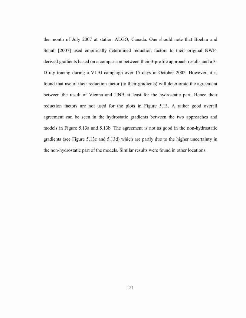
121

the month of July 2007 at station ALGO, Canada. One should note that Boehm and

Schuh [2007] used empirically determined reduction factors to their original NWP-

derived gradients based on a comparison between their 3-profile approach results and a 3-

D ray tracing during a VLBI campaign over 15 days in October 2002. However, it is

found that use of their reduction factor (to their gradients) will deteriorate the agreement

between the result of Vienna and UNB at least for the hydrostatic part. Hence their

reduction factors are not used for the plots in Figure 5.13. A rather good overall

agreement can be seen in the hydrostatic gradients between the two approaches and

models in Figure 5.13a and 5.13b. The agreement is not as good in the non-hydrostatic

gradients (see Figure 5.13c and 5.13d) which are partly due to the higher uncertainty in

the non-hydrostatic part of the models. Similar results were found in other locations.

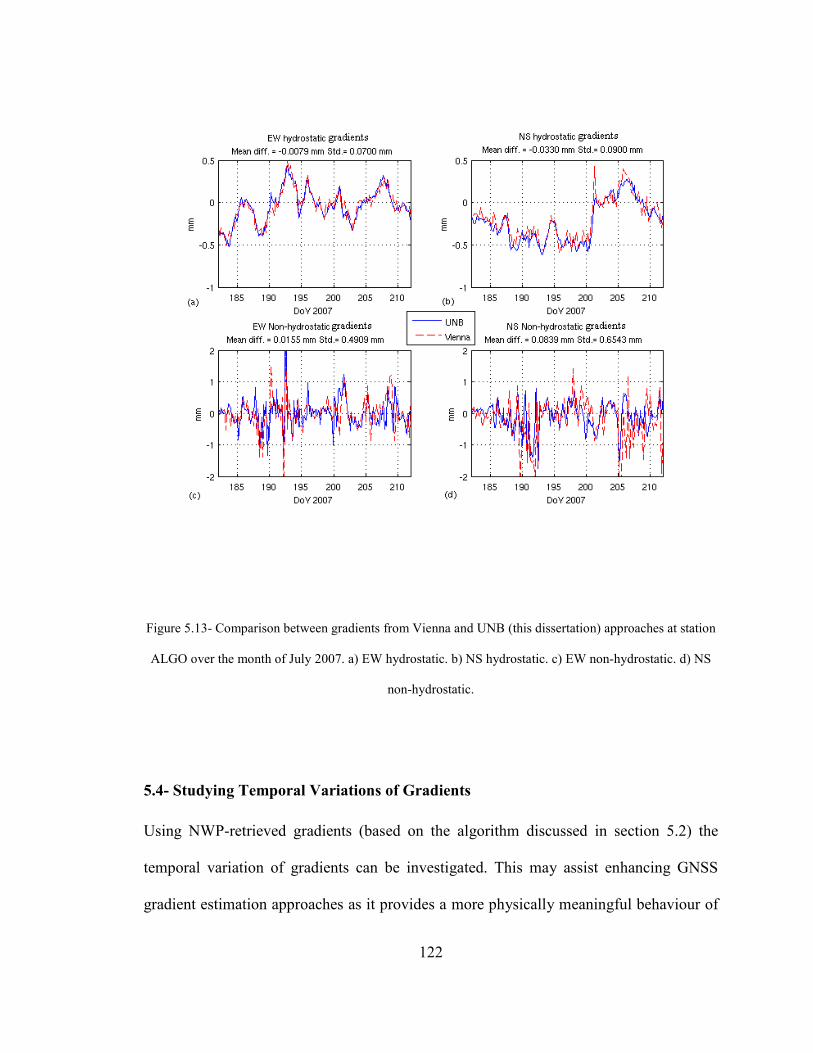
122

Figure 5.13- Comparison between gradients from Vienna and UNB (this dissertation) approaches at station

ALGO over the month of July 2007. a) EW hydrostatic. b) NS hydrostatic. c) EW non-hydrostatic. d) NS

non-hydrostatic.

5.4- Studying Temporal Variations of Gradients

Using NWP-retrieved gradients (based on the algorithm discussed in section 5.2) the

temporal variation of gradients can be investigated. This may assist enhancing GNSS

gradient estimation approaches as it provides a more physically meaningful behaviour of

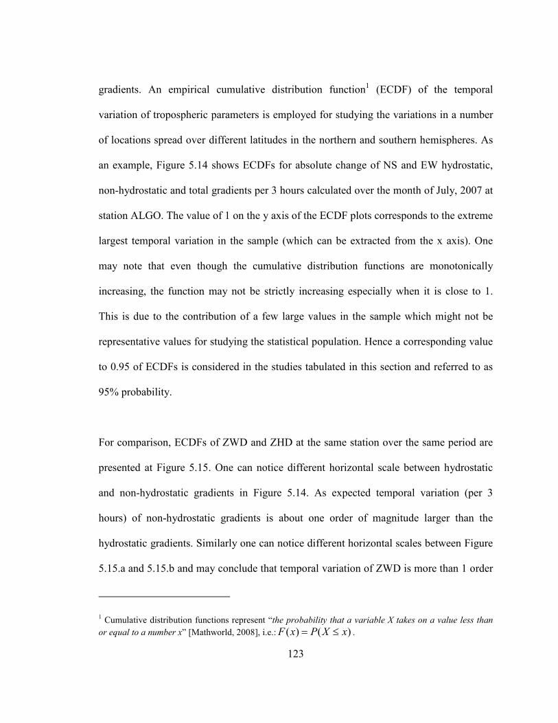
123

gradients. An empirical cumulative distribution function1 (ECDF) of the temporal

variation of tropospheric parameters is employed for studying the variations in a number

of locations spread over different latitudes in the northern and southern hemispheres. As

an example, Figure 5.14 shows ECDFs for absolute change of NS and EW hydrostatic,

non-hydrostatic and total gradients per 3 hours calculated over the month of July, 2007 at

station ALGO. The value of 1 on the y axis of the ECDF plots corresponds to the extreme

largest temporal variation in the sample (which can be extracted from the x axis). One

may note that even though the cumulative distribution functions are monotonically

increasing, the function may not be strictly increasing especially when it is close to 1.

This is due to the contribution of a few large values in the sample which might not be

representative values for studying the statistical population. Hence a corresponding value

to 0.95 of ECDFs is considered in the studies tabulated in this section and referred to as

95% probability.

For comparison, ECDFs of ZWD and ZHD at the same station over the same period are

presented at Figure 5.15. One can notice different horizontal scale between hydrostatic

and non-hydrostatic gradients in Figure 5.14. As expected temporal variation (per 3

hours) of non-hydrostatic gradients is about one order of magnitude larger than the

hydrostatic gradients. Similarly one can notice different horizontal scales between Figure

5.15.a and 5.15.b and may conclude that temporal variation of ZWD is more than 1 order

1 Cumulative distribution functions represent “the probability that a variable X takes on a value less than

or equal to a number x” [Mathworld, 2008], i.e.: )()( xXPxF ≤= .

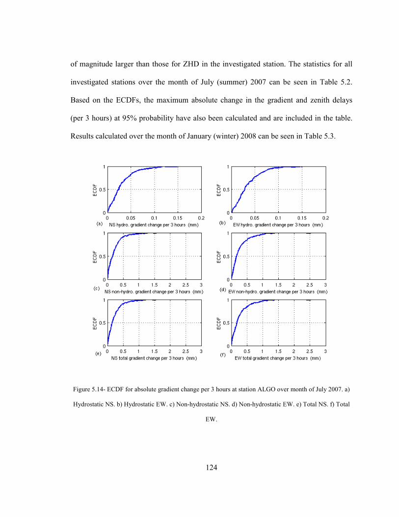
124

of magnitude larger than those for ZHD in the investigated station. The statistics for all

investigated stations over the month of July (summer) 2007 can be seen in Table 5.2.

Based on the ECDFs, the maximum absolute change in the gradient and zenith delays

(per 3 hours) at 95% probability have also been calculated and are included in the table.

Results calculated over the month of January (winter) 2008 can be seen in Table 5.3.

Figure 5.14- ECDF for absolute gradient change per 3 hours at station ALGO over month of July 2007. a)

Hydrostatic NS. b) Hydrostatic EW. c) Non-hydrostatic NS. d) Non-hydrostatic EW. e) Total NS. f) Total

EW.

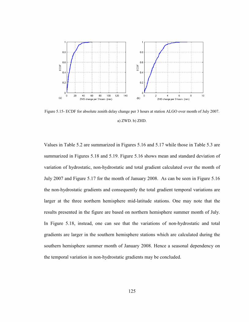
125

Figure 5.15- ECDF for absolute zenith delay change per 3 hours at station ALGO over month of July 2007.

a) ZWD. b) ZHD.

Values in Table 5.2 are summarized in Figures 5.16 and 5.17 while those in Table 5.3 are

summarized in Figures 5.18 and 5.19. Figure 5.16 shows mean and standard deviation of

variation of hydrostatic, non-hydrostatic and total gradient calculated over the month of

July 2007 and Figure 5.17 for the month of January 2008. As can be seen in Figure 5.16

the non-hydrostatic gradients and consequently the total gradient temporal variations are

larger at the three northern hemisphere mid-latitude stations. One may note that the

results presented in the figure are based on northern hemisphere summer month of July.

In Figure 5.18, instead, one can see that the variations of non-hydrostatic and total

gradients are larger in the southern hemisphere stations which are calculated during the

southern hemisphere summer month of January 2008. Hence a seasonal dependency on

the temporal variation in non-hydrostatic gradients may be concluded.

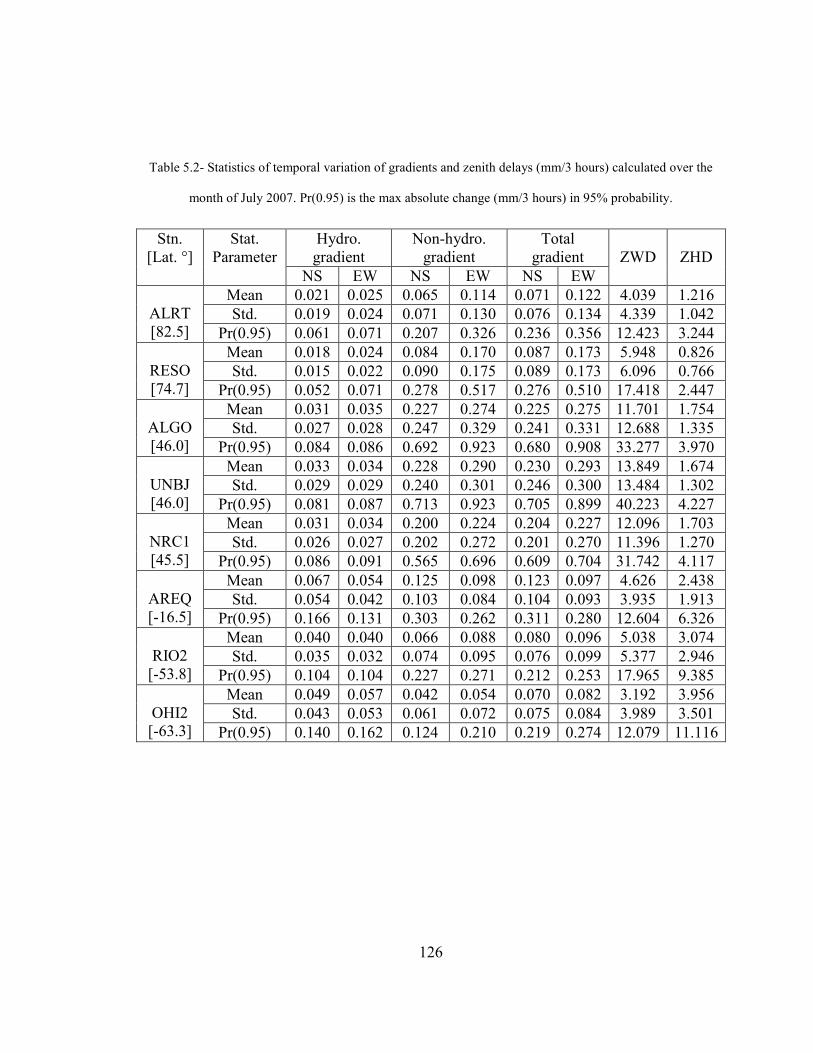
126

Table 5.2- Statistics of temporal variation of gradients and zenith delays (mm/3 hours) calculated over the

month of July 2007. Pr(0.95) is the max absolute change (mm/3 hours) in 95% probability.

Hydro. gradient

Non-hydro. gradient

Total gradient

Stn. [Lat. °]

Stat. Parameter

NS EW NS EW NS EW

ZWD

ZHD

Mean 0.021 0.025 0.065 0.114 0.071 0.122 4.039 1.216 Std. 0.019 0.024 0.071 0.130 0.076 0.134 4.339 1.042

ALRT [82.5] Pr(0.95) 0.061 0.071 0.207 0.326 0.236 0.356 12.423 3.244

Mean 0.018 0.024 0.084 0.170 0.087 0.173 5.948 0.826 Std. 0.015 0.022 0.090 0.175 0.089 0.173 6.096 0.766

RESO [74.7] Pr(0.95) 0.052 0.071 0.278 0.517 0.276 0.510 17.418 2.447

Mean 0.031 0.035 0.227 0.274 0.225 0.275 11.701 1.754 Std. 0.027 0.028 0.247 0.329 0.241 0.331 12.688 1.335

ALGO [46.0] Pr(0.95) 0.084 0.086 0.692 0.923 0.680 0.908 33.277 3.970

Mean 0.033 0.034 0.228 0.290 0.230 0.293 13.849 1.674 Std. 0.029 0.029 0.240 0.301 0.246 0.300 13.484 1.302

UNBJ [46.0] Pr(0.95) 0.081 0.087 0.713 0.923 0.705 0.899 40.223 4.227

Mean 0.031 0.034 0.200 0.224 0.204 0.227 12.096 1.703 Std. 0.026 0.027 0.202 0.272 0.201 0.270 11.396 1.270

NRC1 [45.5] Pr(0.95) 0.086 0.091 0.565 0.696 0.609 0.704 31.742 4.117

Mean 0.067 0.054 0.125 0.098 0.123 0.097 4.626 2.438 Std. 0.054 0.042 0.103 0.084 0.104 0.093 3.935 1.913

AREQ [-16.5] Pr(0.95) 0.166 0.131 0.303 0.262 0.311 0.280 12.604 6.326

Mean 0.040 0.040 0.066 0.088 0.080 0.096 5.038 3.074 Std. 0.035 0.032 0.074 0.095 0.076 0.099 5.377 2.946

RIO2 [-53.8] Pr(0.95) 0.104 0.104 0.227 0.271 0.212 0.253 17.965 9.385

Mean 0.049 0.057 0.042 0.054 0.070 0.082 3.192 3.956 Std. 0.043 0.053 0.061 0.072 0.075 0.084 3.989 3.501

OHI2 [-63.3] Pr(0.95) 0.140 0.162 0.124 0.210 0.219 0.274 12.079 11.116

127

Figure 5.16- Mean and std. of temporal variation of gradients per 3 hours calculated over the month of July

2007. a) Hydrostatic. b) Non-hydrostatic. c) Total. Stations ordered by decreasing latitude.

Figure 5.17 shows the maximum absolute temporal variation of gradients and zenith

delays per 3 hours at 95% probability calculated over the month of July 2007 (Figure

5.19 for month of January 2008). The variations of non-hydrostatic and total gradients are

below 1 mm over 3 hours (at 95% probability) at all stations and in both investigated

summer and winter months. The ZHD and ZWD variations can be seen for comparison in

Figures 5.17d and 5.19d for the months of July 2007 and January 2008 respectively. As

expected, the non-hydrostatic gradient and ZWD temporal variations are larger than the

hydrostatic gradients and ZHD at most stations. This is not as clear for high (low) latitude

stations in northern (southern) hemisphere winter months. This may be due to the low

amount, and variability, of humidity in the winters in the Arctic and Antarctica.

128

Figure 5.17- Maximum absolute temporal variation per 3 hours at 95% probability calculated over the

month of July 2007. a) Hydrostatic gradient. b) Non-hydrostatic gradient. c) Total gradient. d) Zenith delay.

Stations ordered by decreasing latitude.

Although temporal variation of gradients, as well as gradients themselves, depend on

factors such as local weather conditions, topography and mountains1 (which are probably

among the reasons for larger gradient variations at some stations, e.g., AREQ2), a clear

dependence on season and latitude can be concluded from the investigations presented in

Figures 5.16 to 5.19 and Tables 5.2 and 5.3. Furthermore, one may notice a slightly larger

average absolute temporal variation in EW gradients compared to NS gradients. The

larger EW variation might be a reason for not having clear average systematic EW effects

1 Orographic lifting, e.g., which is defined as lifting of air as it travels over a mountain [Ackerman and Knox, 2007] can cause different temperature and humidity in upwind and downwind sides of a mountain and hence it may cause delay gradients. 2 One may also notice a lower variability in zenith delay at station AREQ which is likely to be due to the high altitude of this station (about 2447 m) which causes lower values of ZWD and ZHD as well.

129

as pointed out using the dual ray tracing study reported in section 5.1. The result of the

empirical NWP-based study shown here for gradients and zenith delay temporal

variations can be used to tune GNSS tropospheric parameter estimation strategies as will

be shown in the next section.

Table 5.3- Statistics of temporal variation of gradients and zenith delays (mm/3 hours) calculated over the

month of January 2008. Pr(0.95) is the max absolute change (mm/3 hours) at 95% probability.

Hydro. gradient

Non-hydro. gradient

Total gradient Stn. [Lat.°]

Stat. Parameter

NS EW NS EW NS EW

ZWD

ZHD

Mean 0.027 0.037 0.012 0.024 0.033 0.046 0.665 2.157 Std. 0.024 0.032 0.018 0.032 0.032 0.041 0.790 2.063

ALRT [82.5] Pr(0.95) 0.070 0.094 0.039 0.077 0.088 0.129 2.304 5.947

Mean 0.026 0.033 0.014 0.026 0.031 0.043 0.941 1.627 Std. 0.025 0.033 0.017 0.031 0.029 0.045 1.233 1.879

RESO [74.7] Pr(0.95) 0.074 0.105 0.041 0.086 0.085 0.144 3.278 4.354

Mean 0.048 0.063 0.090 0.107 0.107 0.132 6.172 3.936 Std. 0.039 0.061 0.131 0.185 0.141 0.207 9.167 4.117

ALGO [46.0] Pr(.95) 0.126 0.180 0.347 0.451 0.372 0.532 25.027 11.609

Mean 0.050 0.069 0.101 0.140 0.116 0.167 7.133 4.354 Std. 0.043 0.066 0.123 0.243 0.127 0.266 11.521 4.728

UNBJ [46.0] Pr(0.95) 0.128 0.189 0.326 0.626 0.358 0.553 30.991 11.412

Mean 0.048 0.061 0.092 0.124 0.107 0.146 6.448 3.979 Std. 0.038 0.065 0.145 0.226 0.148 0.239 9.986 4.313

NRC1 [45.5] Pr(0.95) 0.133 0.182 0.374 0.510 0.370 0.657 25.039 10.520

Mean 0.088 0.064 0.341 0.245 0.323 0.235 7.296 2.155 Std. 0.065 0.049 0.276 0.205 0.259 0.202 5.378 1.401

AREQ [-16.5] Pr(0.95) 0.206 0.165 0.867 0.662 0.837 0.632 17.923 4.956

Mean 0.040 0.052 0.160 0.221 0.168 0.228 11.655 2.837 Std. 0.032 0.045 0.183 0.258 0.185 0.265 12.228 2.056

RIO2 [-53.8] Pr(0.95) 0.098 0.135 0.440 0.723 0.447 0.806 37.798 6.955

Mean 0.039 0.057 0.088 0.146 0.100 0.165 6.029 2.943 Std. 0.031 0.054 0.106 0.197 0.114 0.205 6.970 3.320

OHI2 [-63.3] Pr(0.95) 0.101 0.167 0.274 0.514 0.279 0.568 19.775 7.251

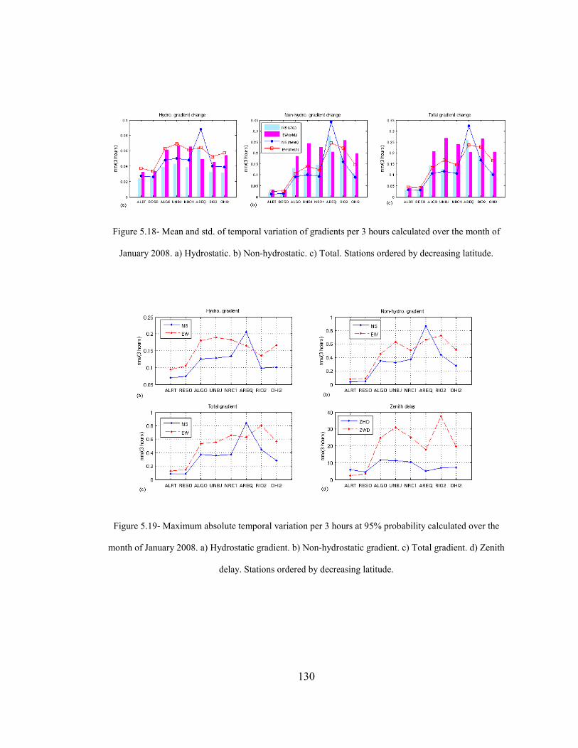
130

Figure 5.18- Mean and std. of temporal variation of gradients per 3 hours calculated over the month of

January 2008. a) Hydrostatic. b) Non-hydrostatic. c) Total. Stations ordered by decreasing latitude.

Figure 5.19- Maximum absolute temporal variation per 3 hours at 95% probability calculated over the

month of January 2008. a) Hydrostatic gradient. b) Non-hydrostatic gradient. c) Total gradient. d) Zenith

delay. Stations ordered by decreasing latitude.

131

5.5- GPS-estimated Gradients

Current scientific GPS software products usually use either stochastic (Kalman filter) or

deterministic (least-squares adjustment) strategies to estimate tropospheric parameters,

including horizontal gradients. The most common estimation strategies and

parameterizations are summarized in Figure 5.20. One may refer to, for example, Gelb

[1974] or Brown and Hwang [1997] for details on stochastic parameter estimation

approaches. As shown in Figure 5.20, a first-order Gauss-Markov process is

parameterized by state variation and correlation time while a random walk process is

parameterized by process noise rate. However, a random walk process can be considered

a special Gauss-Markov process with correlation time of infinity [Dodson et al., 1996]

(e.g. 100 hours for a 24-hour GPS session [GAMIT, 2006]). Furthermore, a piece-wise

linear parameterization when the parameters are assumed to be correlated is roughly

equivalent to a random walk parameterization [Bock and Doerflinger, 2001]. It has been

reported that current approaches of ZTD estimation perform at the same level of accuracy

and precision (see e.g. Ware et al. [1993] and van der Wal [1995]).

132

Figure 5.20- A schematic representation of current GPS tropospheric parameter estimation approaches.

Bernese GPS software Version 5.0 uses a deterministic approach for parameter

estimation by least-squares. In this software the tropospheric zenith delay and gradients

are treated as piece-wise linear parameters. The partial derivatives for tropospheric

parameters (gradients and residual zenith delay) are as follows:

)cos(azz

mfA

nsG ⋅∂∂⋅= γ (5.16)

)sin(azz

mfA

ewG ⋅∂∂⋅= γ (5.17)

mfAZTD ⋅= γ (5.18)

wherensGA ,

ewGA and ZTDA are the partial derivatives for NS gradient, EW gradient and

ZTD respectively; z and az are the zenith angle and azimuth respectively and:

Parameter estimation

Deterministic Stochastic

Piece-wise linear First-order Gauss-Markov

Random walk

-Process noise rate -State variation -Correlation time

Independent Correlated

133

10,1 0 ≤≤∆

−−= γγ

t

tt i (5.19)

where it is the current epoch, 0t is the reference epoch of the estimation interval and t∆ is

the estimation interval. One may note that equations (5.16) and (5.17) result from the idea

of tilting of the atmosphere (see section 3.2.3) where the gradient mapping function is

equivalent to the derivative of a symmetric mapping function with respect to the zenith

angle.

Partial derivatives based on equations (5.16) to (5.19) are calculated for 24 hours of GPS

observations at two stations located at different latitudes. Figures 5.21 and 5.22 are partial

derivatives at station ALGO (a mid-latitude station) vs. elevation angle and time

respectively, with 2 hour tropospheric parameter estimation intervals. Figures 5.23 and

5.24 are those at station ALRT (a high latitude station). Figures 5.21 to 5.24 exemplify

the importance of low elevation angle GPS measurements in the estimation of

tropospheric parameters, as has already been stated by others (e.g. Bar-Sever et al. [1998]

and Meindl et al. [2004]). This can also be explained by the similar partial derivatives of

height and ZTD components at high elevation angles. One may notice from equation

(3.13.c) that the partial derivative for the height component is )sin(/1 ε . For elevation

angles above about 20°, this provides almost the same value as a mapping function. Only

when low elevation angles are used the mapping function (partial derivative of ZTD) is

becoming significantly different than )sin(/1 ε and this can prevent ill-conditioning of the

design matrix. From Figures 5.21 and 5.23 it is clear that observations below 15 degrees

134

are essential for gradient estimation. Furthermore, the GPS constellation (with a lack of

visible satellites in the north direction from mid-latitude) may result in systematic effects

on NS estimated gradients compared to the EW estimated gradients in mid-latitude

stations (compare Figure 5.21a and 5.21b). For the same reason, the accuracy of gradients

estimated at stations in different latitudes may also differ systematically (compare

Figures 5.21 and 5.23 and note the different scales on the y-axes). Low elevation angle

measurements at different azimuths are crucial for estimation of gradients. This fact may

prevent reliable short interval estimation of gradients. In other words, over some short

periods during a session, there may not be enough low elevation quality-control-passed

observations to be used for estimation of gradients.

Figure 5.21- Partial derivative vs. elevation angle calculated for 2 hours estimation intervals at station

ALGO, DoY 197, 2007. a) NS gradient. b) EW gradient. c) ZTD.

135

Figure 5.22- Partial derivative vs. time calculated for 2 hours estimation intervals at station ALGO, DoY

197, 2007. a) NS gradient. b) EW gradient. c) ZTD.

Figure 5.23- Partial derivative vs. elevation angle calculated for 2 hours estimation intervals at station

ALRT, DoY 197, 2007. a) NS gradient. b) EW gradient. c) ZTD.

Figure 5.24- Partial derivative vs. time calculated for 2 hours estimation intervals at station ALRT, DoY

197, 2007. a) NS gradient. b) EW gradient. c) ZTD.

136

5.5.1- Gradient Estimation Interval Effect

Estimation of one set of unconstrained gradients for a 24-hour session has been a

common practice in deterministic piece-wise estimation approaches such as the one used

in Bernese. However, the NWP-based investigation results in the previous section shows

that, depending on the location and season, gradients may vary at the sub-millimetre level

over a much shorter period of time than 24 hours. Compared to the gradient values

themselves the amount of the variation may seem significant. In this section, an

investigation is carried out using the Bernese software to study the effect of shortening

gradient estimation intervals on other estimated parameters including coordinates and

ZTD. Based on the gradient temporal variation studies in the previous section, one may

introduce relative constraints on the gradient to prevent large variations in estimated

gradients. This can also be useful to study the effect of relative constraints on the results.

One month of GPS observations at station ALGO during July 2007 was processed using a

Bernese precise point positioning engine1 with different gradient estimation intervals, and

with and without relative constraints. The relative constraint values are chosen based on

the NWP-based study for the same month and station. The 31 sets of daily coordinates

and 31 sets of 2-hourly ZTD estimates are compared with the International GNSS Service

(IGS) cumulative solution2 and IGS ZTD estimates. The mean and standard deviation of

differences are presented in Table 5.4. As can be seen in Table 5.4, shortening gradient

1 A modified version of the Bernese software capable of using NWP-based zenith delay and mapping function (VMF1) is used here without a priori gradient. See Chapter 6 for details of the modified software. 2 IGS Analysis Centers’ combined cumulative solution up to week 1445.

137

estimation intervals without relative constraints can result in larger standard deviations of

differences from IGS solutions. Standard deviations are smaller when the gradients are

relatively constrained. Based on the RMS of differences from IGS, horizontal and height

components does not seem to be significantly affected (on average over a month) under

different options shown in Table 5.4. However the ZTD estimates seems to be degraded

when gradients were estimated every 2 hours without relative constraining. In this case,

relative constraining has improved the ZTD estimates.

Table 5.4– Statistics of difference between PPP estimation results under various gradient estimation

intervals and IGS solution. Station: ALGO, July, 2007. N/A indicates relative constraining is not applied.

Gradient estimation interval

2 hours

6 hours

Rel. const. 0.3 mm N/A 0.5 mm N/A

Diff. from IGS

Mean (mm)

Std. (mm)

Mean (mm)

Std. (mm)

Mean (mm)

Std. (mm)

Mean (mm)

Std. (mm)

Lat. -2.90 2.63 -2.90 2.63 -2.88 2.59 -2.86 2.59 Lon. 3.70 3.68 3.80 4.00 3.72 3.65 3.91 3.70 Ht. -1.28 6.64 -2.48 6.67 -0.73 7.07 -1.71 7.22 ZTD -3.10 7.50 -1.24 12.70 -3.87 7.08 -2.86 8.46

Gradient estimation interval

12 hours

24 hours

Rel. const. 0.5 mm N/A 0.7 mm N/A

Diff. from IGS

Mean (mm)

Std. (mm)

Mean (mm)

Std. (mm)

Mean (mm)

Std. (mm)

Mean (mm)

Std. (mm)

Lat. -3.01 2.60 -3.00 2.60 -3.01 2.60 -3.01 2.61 Lon. 3.18 3.71 3.10 3.70 3.14 3.72 3.13 3.73 Ht. 0.21 7.07 -0.05 7.20 0.33 6.96 0.31 6.96 ZTD -5.14 6.26 -4.91 6.75 -5.40 5.78 -5.34 5.84

138

5.6- Summary

The behaviour of hydrostatic gradients has been studied in a statistical sense by using

radiosonde data sets. The results showed clear average NS hydrostatic gradients over the

region studied. There was not such a clear trend in EW gradients. For real-time gradients

an algorithm has been developed to retrieve gradients from NWP models. Temporal

variation of gradients and zenith delays were investigated using the NWP-based

approach. The results were used for tuning relative constraints in gradient estimation. In

Chapter 6 implementation of NWP-based gradients, zenith delays and mapping functions

in scientific GNSS software will be discussed.

139

6. Chapter 6: NWP-based Parameters in GPS Software: Analysis

and Results

In this chapter, the use of a semi-3-D NWP-based approach by means of implementing

gradients as a priori to the code pseudorange and phase observations will be discussed.

Modifications that have been carried out on Bernese GPS software to make it capable of

using NWP products in all processing options will be reviewed. The effect of the NWP

implemented option on some pre-processing results will be investigated as well. The

effect of NWP-based parameters on a month long data set at a number of stations was

carried out to investigate the change of GPS-estimated parameters under these

implementations.

6.1- A Semi-3-D NWP-Based Neutral Atmospheric Correction

Although independent observations reported in Chapter 4 show good accuracy of ZHD

derived from NWP models especially in low altitude regions, the accuracy of ZWD

derived from these models is usually far less than that of ZHD. While NWP models

provide a far more realistic 3-D atmospheric structure than standard atmosphere models,

slant delays derived from NWP models are still not accurate enough for high precision

GNSS positioning applications without estimation of residual tropospheric delay. Hence

3-D ray tracing trough NWP models may not be worth the effort.

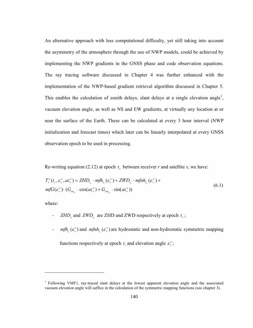
140

An alternative approach with less computational difficulty, yet still taking into account

the asymmetry of the atmosphere through the use of NWP models, could be achieved by

implementing the NWP gradients in the GNSS phase and code observation equations.

The ray tracing software discussed in Chapter 4 was further enhanced with the

implementation of the NWP-based gradient retrieval algorithm discussed in Chapter 5.

This enables the calculation of zenith delays, slant delays at a single elevation angle1,

vacuum elevation angle, as well as NS and EW gradients, at virtually any location at or

near the surface of the Earth. These can be calculated at every 3 hour interval (NWP

initialization and forecast times) which later can be linearly interpolated at every GNSS

observation epoch to be used in processing.

Re-writing equation (2.12) at epoch rt between receiver r and satellite s, we have:

))sin()cos(()(

)()(),,(s

rew

s

rns

s

r

s

rtt

s

rtt

s

r

s

rr

s

r

azGazGmfG

mfnhZWDmfhZHDaztT

rtrt

rrrr

⋅+⋅⋅

+⋅+⋅=

ε

εεε (6.1)

where:

- rt

ZHD and rt

ZWD are ZHD and ZWD respectively at epoch rt ;

- )( s

rtrmfh ε and )( s

rtrmfnh ε are hydrostatic and non-hydrostatic symmetric mapping

functions respectively at epoch rt and elevation angle s

rε ;

1 Following VMF1, ray-traced slant delays at the lowest apparent elevation angle and the associated vacuum elevation angle will suffice in the calculation of the symmetric mapping functions (see chapter 3).

141

- )( s

rmfG ε is the gradient mapping function at elevation angle s

rε (depending on

the gradient mapping function it can be a function of rt too);

- rt

nsG and rt

ewG are NS and EW horizontal gradients at epoch rt ; and

- s

raz is the azimuth between satellite s and receiver r.

As reviewed in Chapter 3 a number of gradient mapping functions have been developed.

Figure 6.1 shows the difference between commonly used gradient mapping functions and

the hydrostatic gradient mapping function of Chen and Herring [1997] referred to as

CH(h). The compared mapping functions include the non-hydrostatic Chen and Herring

(CH(nh)), Davis [1993] with the hydrostatic NMF (Davis(NMFh)), Davis with the non-

hydrostatic NMF (Davis(NMFnh)), and the derivative of the hydrostatic and non-

hydrostatic NMF and VMF1 with respect to zenith angle.

Figure 6.1- Differences of the most commonly used gradient mapping functions from CH(h) during DoY

197, 2007 at station ALGO (Canada). As an example, values in parentheses in the legend are the

differences at 7 degree elevation angle.

142

The large difference between gradient mapping functions at low elevation angles might

be significant. The validation of gradient mapping functions is not a trivial task. Studies

reported in Chapter 5 show that CH(h) and the derivative of non-hydrostatic VMF1

provided closer results to the dual radiosonde ray tracing for hydrostatic asymmetric

delay. One may note that the derivative of VMF1 has the advantage of being a function

of location and the real time of the measurement.

Current strategies for high precision GNSS processing usually down-weight the low

elevation angle measurements by an elevation-angle-dependent function. This makes the

choice of gradient mapping function less critical. A number of authors have reported that

the results of VLBI and GPS are not sensitive to the choice of gradient mapping function

(see e.g. Bock and Doerflinger [2001], Bar-Sever et al. [1998] and MacMillan [1995]).

These references all refer to the effect of the gradient mapping function when it is only

used for estimation of gradients; i.e., as a part of the design matrix. The effect of the

gradient mapping functions in the current approach; i.e., when it is also used to correct

the slant delay a priori (in equation (6.1)) is investigated. Figure 6.2 shows the difference

that using the derivative of the hydrostatic or non-hydrostatic VMF1 as a gradient

mapping function can cause in the slant hydrostatic delays over 24 hours of

measurements. Only 0.15% of measurements in the day were affected by more than 0.5

cm.

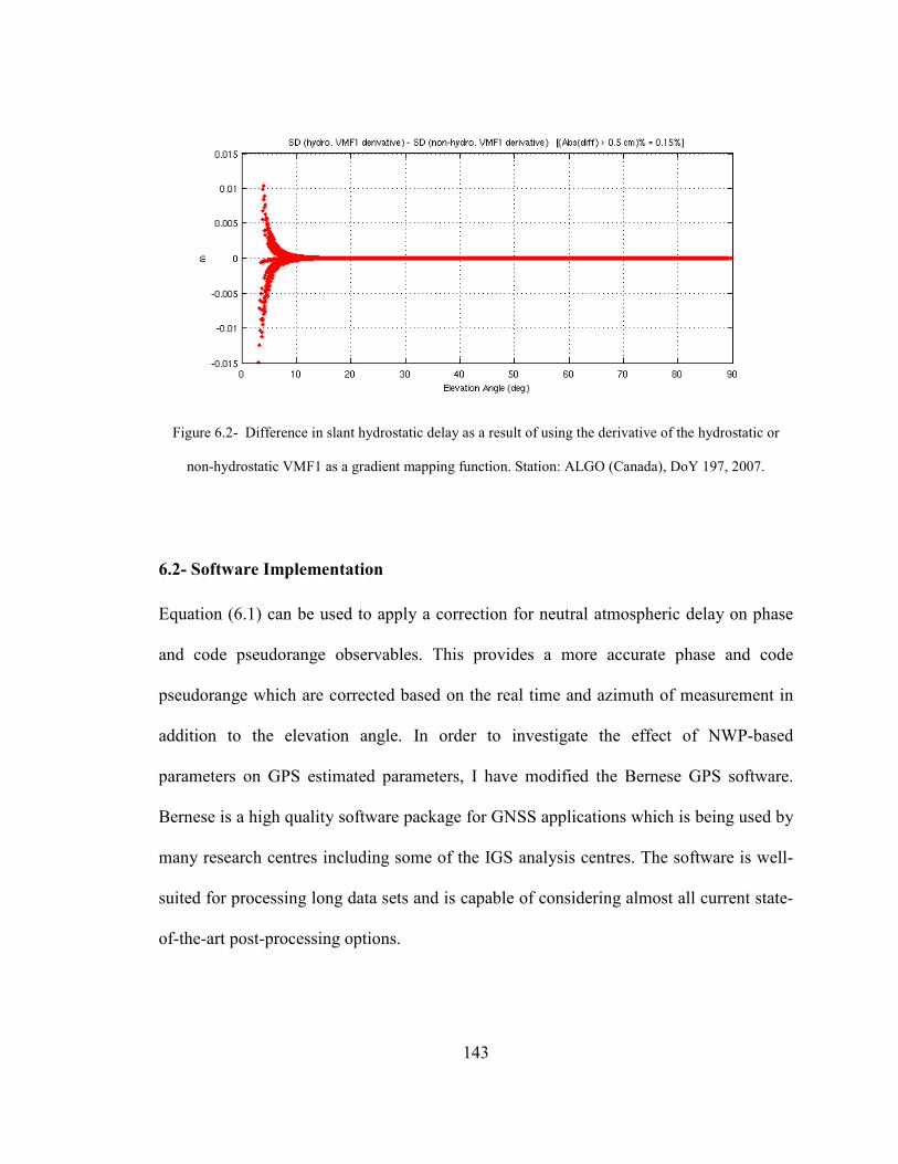
143

Figure 6.2- Difference in slant hydrostatic delay as a result of using the derivative of the hydrostatic or

non-hydrostatic VMF1 as a gradient mapping function. Station: ALGO (Canada), DoY 197, 2007.

6.2- Software Implementation

Equation (6.1) can be used to apply a correction for neutral atmospheric delay on phase

and code pseudorange observables. This provides a more accurate phase and code

pseudorange which are corrected based on the real time and azimuth of measurement in

addition to the elevation angle. In order to investigate the effect of NWP-based

parameters on GPS estimated parameters, I have modified the Bernese GPS software.

Bernese is a high quality software package for GNSS applications which is being used by

many research centres including some of the IGS analysis centres. The software is well-

suited for processing long data sets and is capable of considering almost all current state-

of-the-art post-processing options.

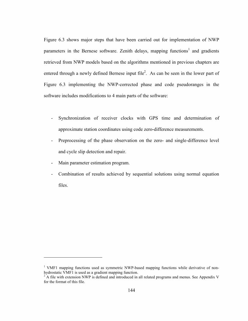
144

Figure 6.3 shows major steps that have been carried out for implementation of NWP

parameters in the Bernese software. Zenith delays, mapping functions1 and gradients

retrieved from NWP models based on the algorithms mentioned in previous chapters are

entered through a newly defined Bernese input file2. As can be seen in the lower part of

Figure 6.3 implementing the NWP-corrected phase and code pseudoranges in the

software includes modifications to 4 main parts of the software:

- Synchronization of receiver clocks with GPS time and determination of

approximate station coordinates using code zero-difference measurements.

- Preprocessing of the phase observation on the zero- and single-difference level

and cycle slip detection and repair.

- Main parameter estimation program.

- Combination of results achieved by sequential solutions using normal equation

files.

1 VMF1 mapping functions used as symmetric NWP-based mapping functions while derivative of non-hydrostatic VMF1 is used as a gradient mapping function. 2 A file with extension NWP is defined and introduced in all related programs and menus. See Appendix V for the format of this file.

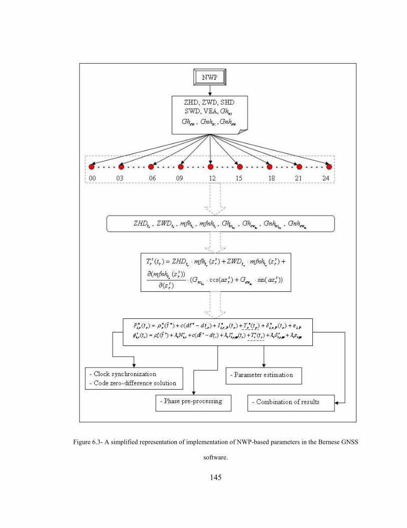
145

Figure 6.3- A simplified representation of implementation of NWP-based parameters in the Bernese GNSS

software.

ZHD, ZWD, SHD SWD, VEA, Gh,.,

Gh.,. , Gnh,., , Gnh.,.

: 00 03 06 09 12 15 18 21 24 : ' ' ---------------------------------------------, -------------------------------------

-

' ' ":,' '::-.... ,' ZHD, , ZWD, , m.fh, , mfnh, , Gil,, , Gh.,. , Gnh,., , Gnh.,.

, , , • .. 4. '" "

' ' ' ' -.. .:... ,·-..~

T,'(t,) = ZHD,, m.Jh,, (z~) +ZWD,, mjnh,, (z:) +

o(mfnh,, (z:)) -----,--",----'--- (G., · ccs(az:) +G.,. sin( az:))

o(z:) •• •

..... : ' -,

P,:,(t,) = p;(t') + c(df'- d~,) + I;,,,,(t,) +_~.~~t~? + o;,,,,(t,) + "'•·•

;~.(t.) = p;(t') + :t,N4, +c(a'-dt.) +:t,I;,,..(t.) + r;(t,) +:!,&,~,.. + :t,e,., -----·

! - Clock synchronization I -Parameter estimation I - Code zero-difference solution

I -Phase pre-processing I I -Combination of results r-

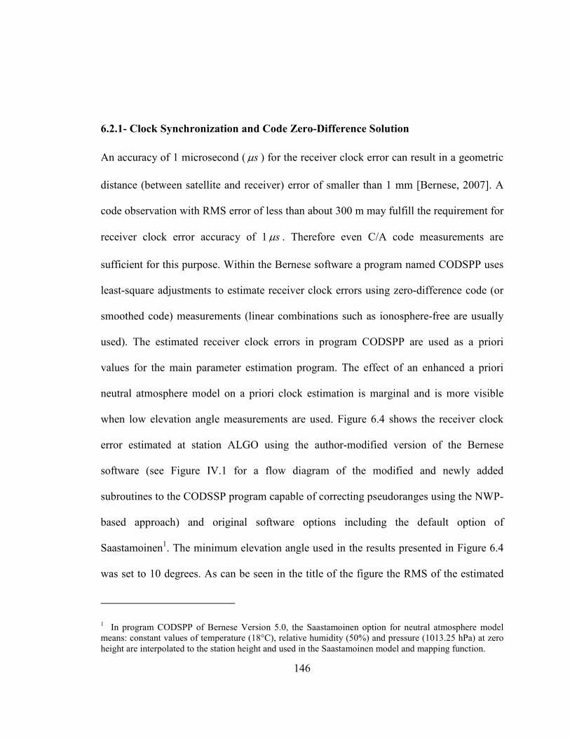
146

6.2.1- Clock Synchronization and Code Zero-Difference Solution

An accuracy of 1 microsecond ( sµ ) for the receiver clock error can result in a geometric

distance (between satellite and receiver) error of smaller than 1 mm [Bernese, 2007]. A

code observation with RMS error of less than about 300 m may fulfill the requirement for

receiver clock error accuracy of 1 sµ . Therefore even C/A code measurements are

sufficient for this purpose. Within the Bernese software a program named CODSPP uses

least-square adjustments to estimate receiver clock errors using zero-difference code (or

smoothed code) measurements (linear combinations such as ionosphere-free are usually

used). The estimated receiver clock errors in program CODSPP are used as a priori

values for the main parameter estimation program. The effect of an enhanced a priori

neutral atmosphere model on a priori clock estimation is marginal and is more visible

when low elevation angle measurements are used. Figure 6.4 shows the receiver clock

error estimated at station ALGO using the author-modified version of the Bernese

software (see Figure IV.1 for a flow diagram of the modified and newly added

subroutines to the CODSSP program capable of correcting pseudoranges using the NWP-

based approach) and original software options including the default option of

Saastamoinen1. The minimum elevation angle used in the results presented in Figure 6.4

was set to 10 degrees. As can be seen in the title of the figure the RMS of the estimated

1 In program CODSPP of Bernese Version 5.0, the Saastamoinen option for neutral atmosphere model means: constant values of temperature (18°C), relative humidity (50%) and pressure (1013.25 hPa) at zero height are interpolated to the station height and used in the Saastamoinen model and mapping function.

147

clock error differences is 0.0012562 sµ . The RMS increased to 0.0015585 sµ when the

minimum elevation angle was decreased to 3 degrees (see Figure 6.5). Some effects

which are likely to be due to the larger errors in low elevation angle measurements under

the Saastamoinen approach can be seen in Figure 6.5. ZHD and ZWD from NWP and

Saastamoinen (as implemented in the original Bernese) at station ALGO in the

investigated day can be seen in Figure 6.6. A clear correlation between the larger ZWD

difference between the two neutral atmospheric modeling approaches from DoY 192 to

192.6 (see Figure 6.6b) and the larger difference between the estimated clocks can be

seen. However it should be mentioned that a priori receiver clock error estimates under

either of the neutral atmospheric modeling strategies are usually sufficiently close to be

able to provide similar final clock and coordinate results from the main parameter

estimation program (in a PPP approach for example).

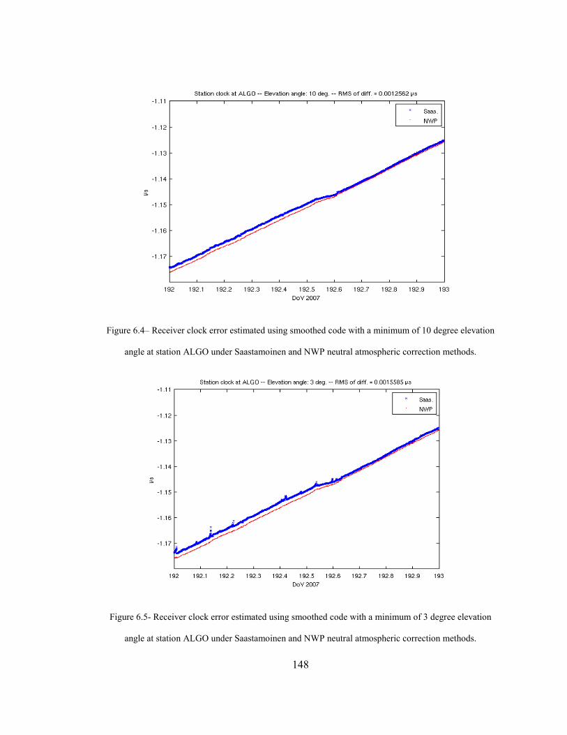
148

Figure 6.4– Receiver clock error estimated using smoothed code with a minimum of 10 degree elevation

angle at station ALGO under Saastamoinen and NWP neutral atmospheric correction methods.

Figure 6.5- Receiver clock error estimated using smoothed code with a minimum of 3 degree elevation

angle at station ALGO under Saastamoinen and NWP neutral atmospheric correction methods.

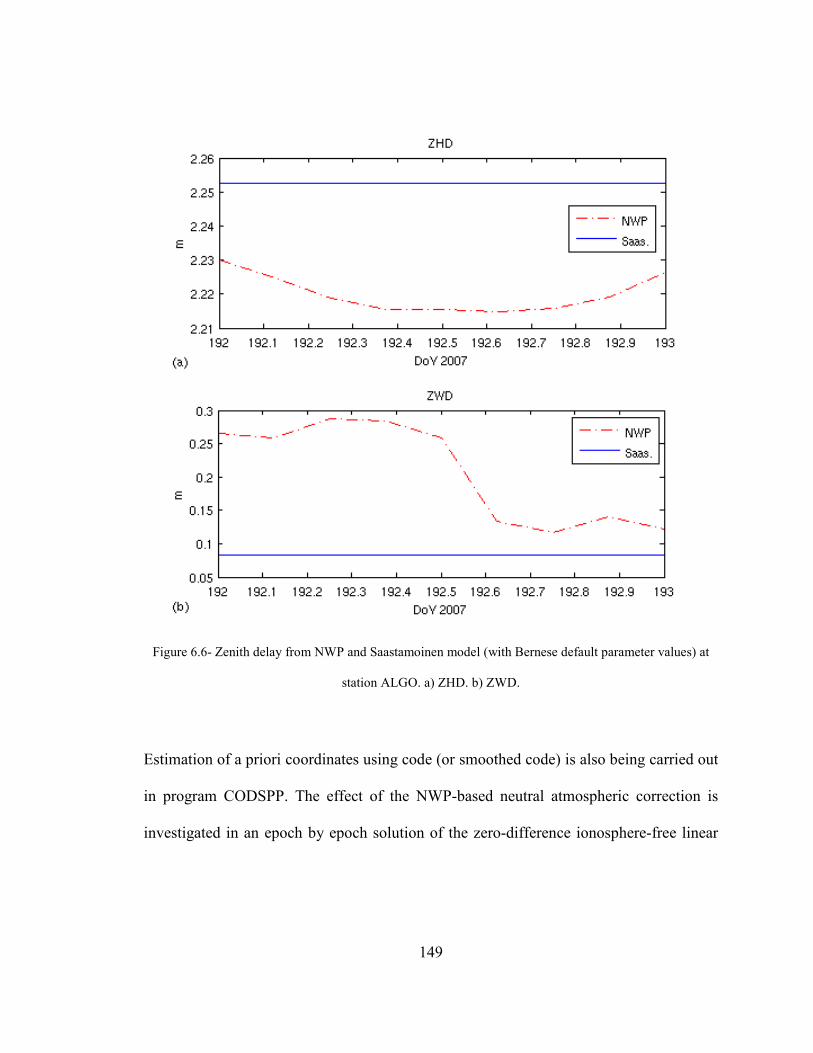
149

Figure 6.6- Zenith delay from NWP and Saastamoinen model (with Bernese default parameter values) at

station ALGO. a) ZHD. b) ZWD.

Estimation of a priori coordinates using code (or smoothed code) is also being carried out

in program CODSPP. The effect of the NWP-based neutral atmospheric correction is

investigated in an epoch by epoch solution of the zero-difference ionosphere-free linear

150

combinations of the smoothed code1 (see equation (2.9) for ionosphere-free linear

combination of code measurements). Figure 6.7 shows coordinate differences from IGS

cumulative solutions2 when an elevation cut off angle of 10° is imposed. The RMS of the

differences can be seen in the title of the subplots. The RMS is smaller when the NWP

option is used, especially in the height component. The results when observations are

down to 3° are processed can be seen in Figure 6.8. The difference between the two

solutions is larger and the effect of the NWP approach becomes more significant. The

large discrepancies of the Saastamoinen solution in some periods in Figure 6.8 are likely

to be due to the low elevation angle measurements which are more vulnerable to an

inaccurate neutral atmosphere modelling. The use of the NWP approach in this

investigated scenario resulted in a decrease of the RMS by about 30 cm in the height

component when low elevation angle measurements are used (see Figure 6.8c). Again

one can notice that the differences between the two solutions are larger during the period

when ZWD values from Saastamoinen differ greatly from the NWP values (compare

Figures 6.6, 6.7 and 6.8). A similar result for smoothed code solutions under different

neutral atmosphere models was found for other stations. Even though the accuracy of

coordinate results from a code solution are not sufficient for high accuracy applications,

improved results under the NWP-based neutral atmospheric modeling approach may be

1 Observation of each satellite arc can be smoothed using the RNXSMT program of Bernese software which employs a number of linear combinations and screening approaches for outliers and cycle slip detection and finally uses carrier phase data to smooth the code data. See Bernese [2007] for details. 2 In this chapter the IGS cumulative solution refers to IGS Analysis Centers’ combined cumulative solution up to week 1445.

151

useful for providing better a priori kinematic coordinates. A least-squares adjustment

approach used in Bernese can be enhanced by improving a priori coordinates.

Figure 6.7– Difference of code solution using Saastamoinen and NWP approaches at station ALGO from

IGS cumulative solution, elevation angle cut off: 10°. a) Latitude. b) Longitude. c) Height.

152

Figure 6.8– Difference of code solution using Saastamoinen and NWP approaches at station ALGO from

IGS cumulative solution, elevation angle cut off: 3°. a) Latitude. b) Longitude. c) Height.

6.2.2- Pre-Processing of Phase Observations

Within the Bernese GPS software a program named MAUPRP is also capable of

identifying cycle slips without the need for code observations. Although this program is

able to process both zero-difference and single-difference observation files, it is not

153

usually used for zero-differences unless high accuracy (better than 0.1 ns) satellite clocks

with the same sampling rate as the observations are available [Bernese, 2007]. The

program performs a number of screening approaches to identify outliers and compute a

triple-difference solution to be used for cycle slip detection.

Hydrostatic, non-hydrostatic and total delay NWP options have been implemented in the

MAUPRP program. In Figure IV.2 the flow diagram of newly added and modified

subroutines in this program are shown. As an example a baseline made by stations ALGO

and NRC1 (about 199 km) was processed using the modified program twice: under the

total delay NWP option and the default option of Niell1. The a priori coordinates of both

stations were chosen from the IGS cumulative solution and station ALGO was considered

as fixed. Assuming the IGS coordinates as true values, the difference between the triple-

difference solution and IGS may represent the accuracy of the solution. Figure 6.9 shows

the NRC1 position difference from IGS (used as a priori) for both solutions. It can be

seen that the NWP option provided more accurate triple-difference solutions.

1 In MAUPRP, Niell option means total zenith delay from Saastamoinen model together with hydrostatic NMF.

154

Figure 6.9– Difference of coordinate components from IGS at NRC1 in a triple-difference solution by

program MAUPRP. Baseline: ALGO-NRC1, DoY 192, 2007.

6.2.3- Main Parameter Estimation

The main parameter estimation program of Bernese, namely GPSEST, sets up the

observation equations and solves the normal equations based on a least-squares approach.

The program deals with the neutral atmospheric delay in two parts: a priori modelling,

and estimation of residual zenith delay and gradients. Similar to the above mentioned

programs, new options have been added to GPSEST for correcting observation equations

based on equation (6.1) where VMF1 (hydrostatic and non-hydrostatic) together with the

derivative of non-hydrostatic VMF1 are used as symmetric and gradient mapping

functions respectively. The possibility of choosing a priori gradients (hydrostatic, non-

hydrostatic or total from NWP) is also provided through the newly defined input file.

155

The hydrostatic and non-hydrostatic VMF1 are added as new options for mapping

functions in order to be used as partial derivatives in the estimation of the residual neutral

atmospheric delay. Figure IV.3 shows a flow diagram of the newly added and modified

subroutines in the GPSEST program. The effect of these added options are partly

investigated in a month-long PPP processing example as will be discussed in section 6.3.

6.2.4- Combination of Solutions

Multi-session solutions are combined in the Bernese software in a program named

ADDNEQ2. The main inputs to this program are the normal equations resulting from the

sequence of solutions from GPSEST. One may refer to Bernese [2007] for details on the

sequential least-squares estimation approach used in ADDNEQ2. Modifications to this

program were carried out to make it capable of handling the results from the modified

GPSEST. Figure IV.4 represents a flow diagram of the modified parts of this program.

6.3- Effect of NWP-Based Corrected Pseudo-ranges on PPP Estimates

As mentioned before, even though NWP models provide a more realistic state of the

atmosphere, due to the uncertainties that are associated with them (especially in the non-

hydrostatic part) the estimation of residual neutral zenith delay is still unavoidable for

high accuracy applications. Hence the hydrostatic zenith delay together with a hydrostatic

mapping function is preferred as an a priori correction. In this case a non-hydrostatic

mapping function can be safely used for the partial derivative for estimation of residuals

156

which, in this case, are the non-hydrostatic delays. In other words, in the absence of an

accurate met sensor collocated with the GNSS antenna, NWP is probably the most

accurate available option for ZHD (see Chapter 4). Hence, the residual outputs can be

considered as ZWD without need for further corrections. Similarly, regarding the use of

NWP-based gradients, it may be more practical to implement hydrostatic gradients rather

than non-hydrostatic or total gradients for two reasons:

1. The higher accuracy of hydrostatic gradients derived from NWP models

compared to the non-hydrostatic gradients.

2. As mentioned in Chapter 5, for GNSS measurements down to a 3 degree elevation

angle, the atmosphere contributing to the hydrostatic path delay has a horizontal

radius of about 700 km around the station. Therefore even low resolution NWP

models may be able to provide useful hydrostatic gradient estimates.

Hence, considering the hydrostatic zenith delay and gradients (and using hydrostatic

VMF1 as a symmetric mapping function and the derivative of the non-hydrostatic VMF1

as a gradient mapping function in equation (6.1)), the a priori slant delay (SD) at epoch i

to satellite j ( j

iSD ) can be written as:

))sin()cos((1

1 j

iEW

j

iNSj

i

j

ij

ii

j

i azGhazGhz

VMFWVMFHZHDSD

ii⋅+⋅

∂

∂+⋅= (6.2)

where iZHD is the zenith hydrostatic delay from the NWP model interpolated to epoch i,

j

iVMFH1 and j

iVMFW1 are the hydrostatic and wet VMF1 (partly from NWP) for

157

satellite j interpolated at epoch i, j

iz and j

iaz are the zenith angle and azimuth at epoch i

to satellite j respectively, and iNSGh and

iEWGh are the hydrostatic NS and EW gradients

from NWP interpolated at epoch i respectively.

Figure 6.10a shows the a priori SD resulting from a standard atmosphere, Saastamoinen

zenith hydrostatic model, and hydrostatic NMF (hereafter referred to as the default) at

station ALGO on DoY 197, 2007. Figure 6.10b shows the difference of SD from NWP

ZHD and VMFH1 (equation (6.2) without gradient components) from the default. Figure

6.10c shows the difference between SD from equation (6.2) and the default. As can be

seen in Figure 6.10b the use of a priori ZHD from NWP caused a difference varying from

10.6 mm to 150 mm with respect to the default scenario (Figure 6.10a) in this case. The

range of differences further increased from 10.5 mm to 179.6 mm when hydrostatic

gradients were also considered. The differences between the NWP option with and

without hydrostatic gradients as a priori can be seen in Figure 6.10d. One might expect

larger differences in situations like the passage of weather fronts or, in case of ZHD,

where the sea-level pressure is very different from that of the standard models used in

GNSS software. One such location is the belt around Antarctica where the annual average

sea-level pressure is of the order of 985 hPa [Peixoto and Oort, 1993], far less than what

is usually considered in models based on a standard atmosphere.

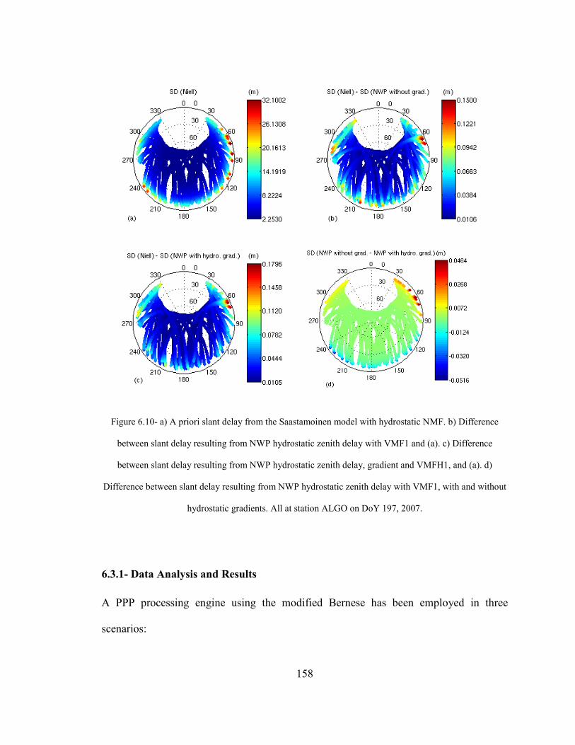
158

Figure 6.10- a) A priori slant delay from the Saastamoinen model with hydrostatic NMF. b) Difference

between slant delay resulting from NWP hydrostatic zenith delay with VMF1 and (a). c) Difference

between slant delay resulting from NWP hydrostatic zenith delay, gradient and VMFH1, and (a). d)

Difference between slant delay resulting from NWP hydrostatic zenith delay with VMF1, with and without

hydrostatic gradients. All at station ALGO on DoY 197, 2007.

6.3.1- Data Analysis and Results

A PPP processing engine using the modified Bernese has been employed in three

scenarios:

159

1. Default processing options: Extrapolated standard constant atmosphere

parameters (see the footnote on section 6.2.1 for constant values) used in the

Saastamoinen model multiplied by the hydrostatic NMF as a priori SD. Non-

hydrostatic NMF used for estimation of ZTD residuals and tropospheric gradients

every 2 and 24 hours respectively.

2. Use of NWP ZHD and hydrostatic VMF1 as a priori SD, non-hydrostatic VMF1

for estimation of ZTD residuals and tropospheric gradients every 2 and 24 hours

respectively.

3. Same as 2 but further correcting the a priori SD by adding NWP hydrostatic

gradients following equation (6.2).

In all scenarios, zero difference ionosphere-free linear combinations of phase and code

were used as the basic observables. While observations down to a 3 degree elevation

angle were used, a weighting function of )(sin 2 e , where e is the elevation angle, was

used to down-weight the low elevation angle measurements. IGS absolute phase-centre

models for satellite and receiver antennas that are dependent on both the elevation angle

and azimuth were used. Schmid et al. [2005] reported that a transition from relative to

absolute phase-centre models could cause jumps of up to 5 mm in the horizontal position

and up to 1 cm in the height component. They also mentioned that an absolute antenna

phase-centre model has the advantage of reducing the dependence of the coordinate

results on the elevation cut-off angle. IGS has switched to an absolute phase-centre model

160

since GPS week 1400 [IGS, 2005]. The antenna phase-centre change, which was carried

out as a part of an updating of the IGS reference frame realization, mainly affects the

height component and caused a decrease of weekly average estimated scale bias [IERS,

2006]. Earth rotation parameters, and final satellite clocks and orbits from IGS were used.

Corrections for ocean tide loading were also applied. RINEX files from the IGS stations

shown in Figure 6.11 covering the whole month of July 2007 were processed three times

according to the above described scenarios. Receiver and antenna types together with

approximate coordinates of the investigated stations are presented in Table 6.1. IGS

cumulative solution and final IGS ZTD1 estimates were adopted for comparisons made in

the rest of this chapter.

The PPP results are from a free network solution and hence the resulting coordinates

share the reference frame defined by the orbits and clocks. Since GPS week 1400, the

IGS products are available in the IGS05 reference frame which is an IGS realization of

the Conventional Terrestrial Reference System. However, one should note that as already

pointed out by others (see e.g. Teferle et al. [2007]), no GPS software is fully consistent

with the combined IGS products. While results presented in this chapter are not from any

kind of transformation between current coordinate results and those of the IGS, the

statistics regarding differences with respect to IGS cumulative solutions may be

considered as a reference for inter-comparison.

1 Final IGS ZTD estimates are at 5 minute intervals provided by Jet Propulsion Laboratory.

161

Figure 6.11- Location of investigated stations.

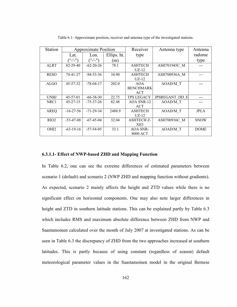
162

Table 6.1- Approximate position, receiver and antenna type of the investigated stations.

Approximate Position Station Lat. (°-'-")

Lon. (°-'-")

Ellips. ht. (m)

Receiver type

Antenna type Antenna radome type

ALRT 82-29-40 -62-20-26 78.1 ASHTECH UZ-12

ASH701945C_M ---

RESO 74-41-27 -94-53-36 34.90 ASHTECH UZ-12

ASH700936A_M ---

ALGO 45-57-32 -78-04-17 202.0 AOA BENCHMARK

ACT

AOAD/M_T ---

UNBJ 45-57-01 -66-38-30 22.75 TPS LEGACY JPSREGANT_DD_E --- NRC1 45-27-15 -75-37-26 82.48 AOA SNR-12

ACT AOAD/M_T ---

AREQ -16-27-56 -71-29-34 2488.9 ASHTECH UZ-12

AOAD/M_T JPLA

RIO2 -53-47-08 -67-45-04 32.04 ASHTECH Z-XII3

ASH700936C_M SNOW

OHI2 -63-19-16 -57-54-05 33.1 AOA SNR-8000 ACT

AOAD/M_T DOME

6.3.1.1- Effect of NWP-based ZHD and Mapping Function

In Table 6.2, one can see the extreme differences of estimated parameters between

scenario 1 (default) and scenario 2 (NWP ZHD and mapping function without gradients).

As expected, scenario 2 mainly affects the height and ZTD values while there is no

significant effect on horizontal components. One may also note larger differences in

height and ZTD in southern latitude stations. This can be explained partly by Table 6.3

which includes RMS and maximum absolute difference between ZHD from NWP and

Saastamoinen calculated over the month of July 2007 at investigated stations. As can be

seen in Table 6.3 the discrepancy of ZHD from the two approaches increased at southern

latitudes. This is partly because of using constant (regardless of season) default

meteorological parameter values in the Saastamoinen model in the original Bernese

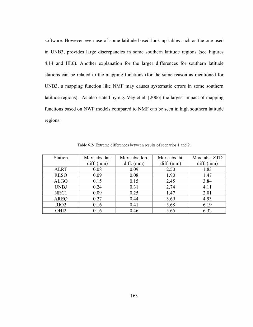
163

software. However even use of some latitude-based look-up tables such as the one used

in UNB3, provides large discrepancies in some southern latitude regions (see Figures

4.14 and III.6). Another explanation for the larger differences for southern latitude

stations can be related to the mapping functions (for the same reason as mentioned for

UNB3, a mapping function like NMF may causes systematic errors in some southern

latitude regions). As also stated by e.g. Vey et al. [2006] the largest impact of mapping

functions based on NWP models compared to NMF can be seen in high southern latitude

regions.

Table 6.2- Extreme differences between results of scenarios 1 and 2.

Station Max. abs. lat. diff. (mm)

Max. abs. lon. diff. (mm)

Max. abs. ht. diff. (mm)

Max. abs. ZTD diff. (mm)

ALRT 0.08 0.09 2.50 1.83 RESO 0.09 0.08 1.90 1.47 ALGO 0.15 0.15 2.45 3.84 UNBJ 0.24 0.31 2.74 4.11 NRC1 0.09 0.25 1.47 2.01 AREQ 0.27 0.44 3.69 4.93 RIO2 0.16 0.41 5.68 6.19 OHI2 0.16 0.46 5.65 6.32

164

Table 6.3- RMS and max. abs. diff. between ZHD from NWP and Saastamoinen calculated over month of

July 2007 at the investigated stations.

Station RMS diff. (mm) Max. abs. diff. (mm) ALRT 10.4 27.7 RESO 13.8 26.4 ALGO 16.5 38.0 UNBJ 14.0 28.9 NRC1 16.1 37.5 AREQ 36.2 45.8 RIO2 39.6 110.9 OHI2 50.8 124.9

6.3.1.2- Effect of NWP-based A Priori Hydrostatic Gradients

As an example, the EW and NS hydrostatic gradients estimated from the NWP model at

ALGO over the month of July 2007 are presented in Figures 6.12a and 6.12b

respectively. Rapid changes of hydrostatic gradients are likely to be a result of the

passage of low or high pressure systems around the investigated location. By taking a

closer look at Figure 6.12b one can notice, for example, a rapid change of the NS

hydrostatic gradient from about -0.5 to 0 mm during 19 to 20 July (DoY 200.5 to 201.5)

at station ALGO. Surface weather maps at these two days are presented in Figures 6.13

and 6.14 while the thickness of the atmosphere between the 500 and 1000 hPa isobaric

levels (hereafter referred to as thickness) and mean sea level (MSL) pressure maps

produced using the Meteorological Service of Canada regional NWP model are also

presented in Figures 6.15 and 6.16. Passage of a cold front from north to south and a low

pressure system near the location of ALGO can be seen in Figure 6.13 and are likely to

be partly responsible for the NS gradient on that day. Features in thickness and MSL

165

pressure maps may be more correlated with hydrostatic gradients. As can be seen in

Figure 6.14a, during DoY 200, the thickness is changing in an NS direction near the

location of ALGO. Furthermore a low MSL pressure area exists at this location while a

higher pressure area is located toward the north of the station (see Figure 6.15b). These

are likely to be the reason for the considerable NS gradient at ALGO. During DoY 201,

however, the edge of thickness change moves further to the south (see Figure 6.15a) and

a low pressure system moves to the east of ALGO (see Figure 6.16b) resulting in a

slightly increased EW hydrostatic gradient which has been quantified by the gradient

estimation algorithm and can be seen in Figure 6.12a.

Figure 6.12- NWP hydrostatic gradients at station ALGO over month of July 2007; a) EW b) NS.

166

The effect of these gradients on daily estimated coordinates and 2-hour ZTD estimates

can be seen in Figures 6.17 to 6.19. Figure 6.17a shows the correlation between latitude

differences resulting from scenarios 3 and 2 (processing with and without hydrostatic

gradients) and the magnitude of hydrostatic gradients. Figure 6.17b shows the correlation

between latitude differences and NS hydrostatic gradients. Figures 6.17c and 6.17d show

the correlations with longitude and height component differences respectively. It is clear

from Figure 6.17b that there is a strong correlation between NS hydrostatic gradients and

latitude differences. No such correlation exists with EW hydrostatic gradients as can be

seen in Figures 6.18a to 6.18c. This may be partly explained by the effect of the GPS

satellites’ sky distribution. Regarding ZTD differences, one can see in Figures 19a to 19c

that NS gradients have a higher correlation with ZTD differences than EW gradients and

magnitudes at this station, although this is much lower than the latitude correlation shown

in Figure 6.17b.

167

Figure 6.13- Surface weather map on DoY 200, 2007 (from NCDC [2008a]).

Statistics for all investigated stations are presented in Table 6.4, which includes

correlation coefficients of the estimated daily coordinate absolute differences between

scenarios 2 and 3 and absolute mean daily NS and EW hydrostatic gradients. Also

included are correlation coefficients of absolute ZTD differences and absolute NS and

EW hydrostatic gradients.

The significance of all correlation coefficient values have been tested using the following

statistic (see e.g. Spiegel and Stephens [1998]):

168

21

2

r

Nrt

−

−⋅= (6.3)

where r is the sample correlation coefficient, and N is the number of values. The statistic

in equation (6.3) has the Student’s distribution with N-2 degrees of freedom. Correlation

coefficients significantly different than zero at a 0.05 significance level, are presented in

bold font in Table 6.4. As can be seen in the table, for all investigated stations there is a

significant and strong correlation between NS hydrostatic gradients and latitude

differences. For most stations, longitude components have not been affected significantly

with the implementation of gradients. The height component and ZTD are also affected

but the correlations with implemented gradients are not as strong as those with latitude,

as previously mentioned.

169

Figure 6.14- Surface weather map on DoY 201, 2007 (from NCDC [2008a]).

170

Figure 6.15- a) Thickness and b) MSL pressure maps produced using Meteorological Service of Canada

regional NWP model on DoY 200.5, 2007.

Thickness (500 hPa- 1000 hPa) at 12 UTC 19-Jul-2007 m

-1000

-2000

~ -3000

-4000

-5000

(a) -2000 -1000

0

-1000

-2000

~ -3000

-4000

-5000

(b) -2000 -1000

0

0

1 000 2000 3000 4000

km

1 000 2000 3000 4000

km

hPa

025

020

015

010

005

000

171

Figure 6.16- a) Thickness and b) MSL pressure maps produced using Meteorological Service of Canada

regional NWP model on DoY 201.5, 2007.

0

-1000

-2000

~ -3000

-4000

-5000

(a) -2000 -1000 0 1 000 2000 3000 4000

km

MSL pressure at 12 UTC 20-Ju1-2007 0

-1000

-2000

~ -3000

-4000

-5000

(b) -2000 -1000 0 1 000 2000 3000 4000

km

hPa

030

025

020

015

010

005

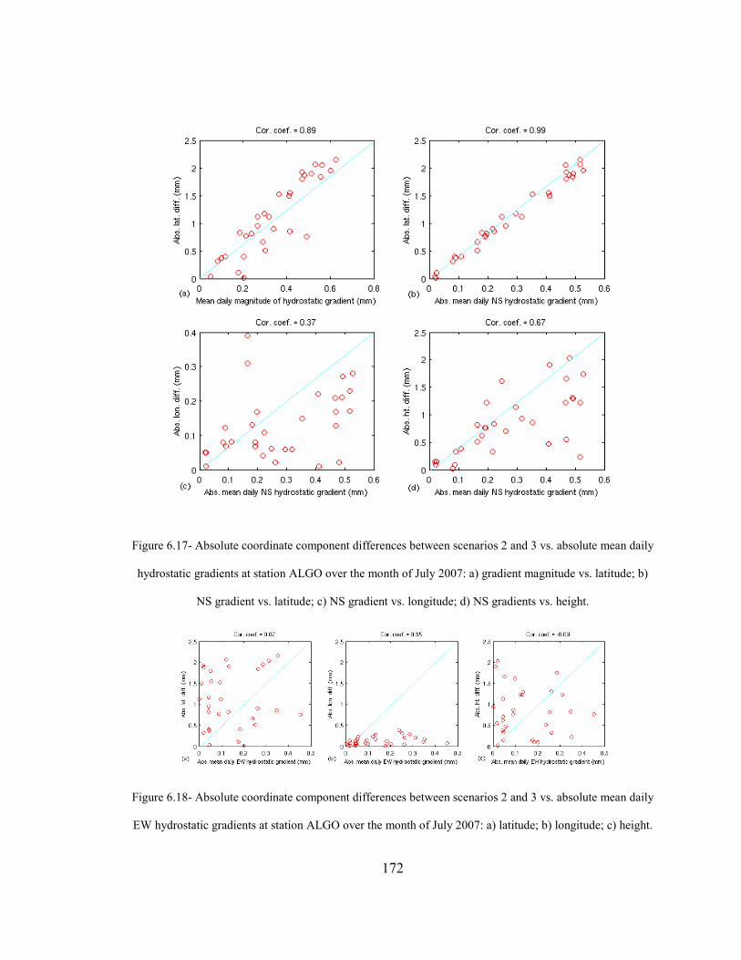
172

Figure 6.17- Absolute coordinate component differences between scenarios 2 and 3 vs. absolute mean daily

hydrostatic gradients at station ALGO over the month of July 2007: a) gradient magnitude vs. latitude; b)

NS gradient vs. latitude; c) NS gradient vs. longitude; d) NS gradients vs. height.

Figure 6.18- Absolute coordinate component differences between scenarios 2 and 3 vs. absolute mean daily

EW hydrostatic gradients at station ALGO over the month of July 2007: a) latitude; b) longitude; c) height.

173

Figure 6.19- Absolute ZTD differences between scenarios 2 and 3 vs. absolute hydrostatic gradients at

station ALGO over the month of July 2007: a) magnitude; b) NS; c) EW.

Table 6.4- Statistics of the comparisons between scenarios 2 and 3.

Lat. Lon. Ht. ZTD Station Corr. with abs. mean daily NS grad.

Corr. with abs. mean daily EW grad.

Abs. max. diff. (mm)

Corr. with abs. mean daily NS grad.



Corr. with abs. mean daily NS grad.



Corr. with abs. NS grad.

Corr. with abs. EW grad.


ALRT 0.99 -0.04 3.39 0.87 0.03 0.86 0.82 0.13 4.41 0.48 0.03 7.43 RESO 0.98 -0.03 1.42 0.20 0.27 0.26 0.77 0.17 3.03 0.27 0.18 1.84 ALGO 0.99 0.07 2.15 0.37 0.35 0.39 0.67 -0.09 2.03 0.55 0.03 2.28 UNBJ 0.98 0.42 2.72 0.28 0.19 0.78 0.45 0.38 2.46 0.40 0.22 3.97 NRC1 0.99 0.19 2.25 0.20 -0.08 0.32 0.78 0.06 2.45 0.57 0.14 2.23 AREQ 0.83 0.25 0.67 0.26 0.17 1.11 0.31 0.51 2.83 0.10 0.14 6.04 RIO2 0.99 -0.02 5.14 0.13 -0.41 1.63 0.55 0.02 3.32 0.59 -0.04 3.04 OHI2 0.99 -0.01 3.78 0.19 0.57 1.35 0.53 -0.27 3.41 0.74 -0.04 4.62

Mean monthly differences between results from the three scenarios and IGS results have

also been investigated. The results from all 3 scenarios agree with the IGS cumulative

estimates in all three components at the mm level (except for station AREQ whose rather

larger differences need further investigation). Tables 6.5 to 6.7 include mean and

174

standard deviation of estimated parameters from the scenarios (except for station RIO2

which did not have an IGS cumulative solution) and those of the IGS. These are also

shown in Figure 6.19 to 6.22. While in a monthly comparison most of the NWP

parameters’ effects might average out, at some stations (namely ALGO, UNBJ, NRC1

and OHI2) the third scenario (NWP with hydrostatic gradients) still caused millimetre

level mean latitude differences compared to the other scenarios. This may indicate that

hydrostatic gradients can have systematic effects on long term latitude estimates.

Table 6.5- Statistics of scenario 1 results vs. IGS values.

Mean diff. from IGS (mm) Std of diff from IGS (mm) Station Lat. Lon. Ht. ZTD Lat. Lon. Ht. ZTD

ALRT 0.41 -4.61 -6.8 0.87 3.59 1.76 10.12 3.98 RESO -3.66 -1.86 -4.77 -2.44 2.43 2.80 8.82 4.30 ALGO -2.99 3.16 -0.47 -3.83 2.61 3.72 7.10 6.00 UNBJ -2.44 -7.03 -6.10 5.66 3.76 3.64 6.87 8.89 NRC1 -2.51 1.06 -4.69 1.86 2.87 3.42 8.16 6.42 OHI2 5.91 1.90 -7.08 4.23 3.57 6.31 12.27 6.70


Mean diff. from IGS (mm) Std. of diff. from IGS (mm) Station Lat. Lon. Ht. ZTD Lat. Lon. Ht. ZTD

ALRT 0.44 -4.61 -6.60 0.47 3.59 1.76 10.02 3.77 RESO -3.66 -1.87 -4.77 -2.67 2.43 2.80 8.64 4.34 ALGO -3.01 3.13 0.31 -5.34 2.61 3.73 6.96 5.84 UNBJ -2.39 -6.97 -5.95 5.02 3.77 3.67 6.99 8.53 NRC1 -2.53 1.16 -4.67 1.20 2.86 3.40 8.07 6.37 OHI2 5.88 1.94 -5.03 1.15 3.58 6.31 11.65 6.05

175


Mean diff. from IGS (mm) Std of diff. from IGS (mm) Station Lat. Lon. Ht. ZTD Lat. Lon. Ht. ZTD

ALRT 0.56 -4.67 -6.60 0.57 3.05 1.84 10.09 3.91 RESO -3.86 -1.86 -5.10 -2.54 2.38 2.77 8.70 4.28 ALGO -2.12 3.14 -0.19 -5.07 2.62 3.75 6.93 5.71 UNBJ -1.08 -7.23 -6.63 5.17 3.81 3.61 6.98 8.53 NRC1 -1.49 1.16 -5.44 1.63 2.68 3.36 7.68 6.35 OHI2 4.25 1.73 -6.14 2.61 3.23 6.25 11.31 5.86

Figure 6.20- Absolute mean and std. of latitude difference between the results of the three scenarios and

IGS values.

176

Figure 6.21- Absolute mean and std. of longitude difference between the results of the three scenarios and

IGS values.

Figure 6.22- Absolute mean and std. of height difference between the results of the three scenarios and IGS

values.

177

Figure 6.23- Absolute mean and std. of ZTD difference between the results of the three scenarios and IGS

values.

6.3.2- Discussion

Estimated parameters from the PPP scenarios show strong correlation between NS

hydrostatic gradients and latitude differences at all investigated stations. A 0.5 mm

absolute mean daily NS gradient at station ALGO, for example, resulted in about 2 mm

latitude difference. Overall, mean ratios of about 4-6 were found between the absolute

latitude difference and the absolute mean daily NS gradient at all investigated stations.

Weaker but still significant correlations also exist between NS gradients and both height

and ZTD. Among the estimated parameters, longitude was the one with least change

178

under implementation of gradients. Although NS and EW hydrostatic gradients are of the

same order of magnitude, the NS gradients seem to have a systematic behaviour as was

studied in Chapter 5.

Monthly averaged estimated parameters show minor changes under the different

scenarios considered. This change is larger for the latitude component at most stations.

The monthly mean latitude results are closer to the reference (IGS) values when the

hydrostatic gradients implemented as a priori (except for the two high latitude stations

where the monthly mean NS hydrostatic gradients were close to zero and no significant

mean latitude differences were found). The standard deviations of latitude, height and

ZTD differences from IGS values slightly decrease at most stations when the third

scenario (NWP with gradients) is used. Based on the estimation algorithms employed in

the Bernese software and PPP results reported in this chapter, implementing hydrostatic

gradients as a priori can cause millimetre level improvement in long term positioning at

least for the latitude component. Estimation of at least one set of gradients per 24 hours

still seems beneficial to absorb the non-hydrostatic gradients.

179

7. Chapter 7: Conclusions and Recommendations

In this dissertation, recent developments in neutral atmospheric modelling using NWP

models have been reviewed. The performance of Canadian NWP models were validated

using independent approaches at different locations including the Canadian Arctic. These

include the use of a WVR and precise barometer on a moving platform in Canadian high

latitudes, comparison with radiosonde data sets, and routine 3-hourly comparison of

NWP and climate-based models. In general, uncertainties of 0.04-0.08% and a 5-10% for

NWP-based ZHD and ZWD respectively can be expected.

The online ray tracing service developed as a part of this research is an example of a

NWP-for-GNSS operational service. Generated near-real-time maps as a part of this

service is an example of the feasibility of NWP models for zenith delay corrections on a

global scale. The performance of UNB’s widely used climate-based models can be

monitored on a routine basis with NWP-based generated maps.

Behaviour of hydrostatic gradients has been studied in a statistical sense by using

radiosonde data sets. The results showed clear average NS hydrostatic gradients over the

region studied. There was not such a clear trend in EW gradients. For real-time gradients

an algorithm has been developed to retrieve gradients from NWP models. The algorithm

uses NWP profiles in all 4 cardinal directions around the station. In order to show the

180

effect of NWP-based parameters on GPS estimates as well as the practicality of the

approach in real applications, the Bernese GPS software has been modified to be able to

handle NWP-based zenith delays, mapping functions and gradients in all related

programs and subroutines. This made the software capable of using a priori NWP data in

all processing options. The modified software provides an eligible tool for research on the

effect of enhanced neutral atmosphere information on the pre- and final processing of

GNSS data.

The effect of NWP-based parameters on a month-long dataset of observations from a

number of stations spread over northern and southern hemispheres was investigated in

three different PPP scenarios. The processing strategies differ in the a priori hydrostatic

slant delay handling. The results show strong correlation between NS hydrostatic

gradients and latitude differences with weaker correlation between NS hydrostatic

gradients and both height component and ZTD differences. Even though NS and EW

gradients are the same order of magnitude it is found that longitude is not sensitive to

either of the hydrostatic gradient components. The effect of ZHD and mapping function

values from NWP when the gradients are not implemented was only seen on height and

ZTD estimates. The largest effect of NWP-based ZHD and mapping functions was found

for southern latitude stations.

Based on the processing results at the investigated stations mean ratios of about 4-6 were

found between absolute latitude difference and absolute mean daily NS gradient. For

181

example, the estimated latitude component could be affected by more than 2 mm as a

result of a 0.5 mm a priori NS hydrostatic gradient. Although the effect in terms of

absolute maximum value might be larger for height and ZTD, the correlation of those

with either gradient component was not as clear as the correlation with latitude.

Furthermore, this may partly be due to higher uncertainty in height and ZTD estimations

compared to horizontal components.

While it is shown in this dissertation that correcting the a priori SD with hydrostatic

gradients can have a millimetre level effect in some estimated components, the modified

Bernese software is capable of considering NWP hydrostatic, non-hydrostatic and total

gradients as a priori in GPS observables as well as zenith delay and mapping functions

based on NWP models in all processing strategies. Considering such effects on latitude,

height and ZTD estimates might be crucial in applications such as deformation

monitoring, long term geodynamic and crustal movements studies, sea-level change

monitoring, defining terrestrial reference frames and climatology and consequential

interpretations. Hence implementing hydrostatic gradients as a priori values is

recommended in GPS processing when the highest accuracy is required in long-term

positioning. Furthermore, in the event of passage of a weather front, the use of NWP-

based parameters can provide more reliable solutions.

A clear dependence of the temporal variation of gradients on season and latitude has been

found based on the NWP-based gradient retrieval approach. Furthermore, a slightly larger

182

average absolute temporal variation in EW gradients compared to NS gradients was

found. This can probably be explained by the unsystematic average EW gradient

behaviour. It was found that shortening the gradient estimation interval (to 12 hours and

less) in the Bernese software decreases the precision of the estimated parameters.

Relative constraining of gradients based on the NWP-based studies may prevent a

degradation of the solution.

Although the UNBgr model, which has been derived from radiosonde data sets in part of

North America, is a monthly averaged model without dependence on location,

implementing this model as a correction to pseudoranges might be a simpler alternative

to the NWP-based gradient approach. This might only be beneficial if long term (longer

than a month) static data sets are needed to be processed and has yet to be investigated.

Other approaches for real-time access to neutral atmosphere corrections such as IP data

streaming may be considered in the future as an alternative to the current online ray

tracing service. A potential future use of the zenith delay map generation service could be

in InSAR applications where a high resolution weather model can be used to reduce the

atmospheric effect on InSAR interferograms.

The effect of current implementations on different processing strategies, and the use of

higher resolution NWP models in order to investigate the effect of local weather

anomalies, are among the future works that could be carried out with the modified

183

Bernese software. Another recommendation for future work is the enhancement of

gradient estimation approaches by choosing modified process noise values by empirical

determination from the NWP-based approach developed in this dissertation. If applicable,

depending on the estimation algorithm, an investigation of the use of higher order

functions rather than piece-wise linear ones in the gradient estimation might improve the

resultant gradients and other estimates.

184

References

Ackerman, S.A., and J.A. Knox (2007). Meteorology: Understanding the Atmosphere. 2nd ed., Thomson Brooks/Cole, Belmont, CA. AMS (2007). Glossary of Meteorology. American Meteorological Society. [On-line] 6 April 2007. http://amsglossary.allenpress.com/glossary Andrews, D.G. (2000). An Introduction to Atmospheric Physics. 1st ed., Cambridge University Press, Cambridge. Baby, H.B., P. Golé, and J. Lavergnat (1988). “A model for the tropospheric excess path length of radio waves from surface meteorological measurements.” Radio Science, Vol. 23, No. 6, pp. 1023-1038. Bar-Sever, Y.E., P.M. Kroger, and J.A. Borjesson (1998). “Estimating horizontal gradients of tropospheric path delay with a single GPS receiver” Journal of Geophysical

Research. Vol. 103, No. B3, pp. 5019-5035. Bean, B.R., and E.J. Dutton (1966). Radio Meteorology. National Bureau of Standards Monograph 92, Government Printing Office, Washington D.C. Bernese (2007). User manual of the Bernese GPS Software Version 5.0. Edited by: Dach, R., U. Hugentobler, P. Fridez and M. Meindl, Astronomical Institute, University of Bern, Bern, Switzerland, 612 pp. Bevis, M., S. Businger, S. Chiswell,T. Herring, R.A. Anthes, C. Rocken, and R.H Ware (1994). GPS meteorology: mapping zenith wet delays onto precipitable water, Journal of Applied Meteorology, Vol. 33, No. 3, 379-386. Bock, O., and E. Doerflinger (2001). Atmospheric modeling in GPS data analysis for high accuracy positioning. Phys. Chem. Earth (A), Vol. 26 No. 6-8, pp. 373-383. Boehm, J., R. Heinkelmann, and H. Schuh (2007a). “Short Note: A global model of pressure and temperature for geodetic applications.” Journal of Geodesy, Vol. 81, pp. 679-683, DOI: 10.1007/s00190-007-0135-3. Boehm, J., P.J. Mendes-Cerveira, Schuh, H., and P. Tregoning (2007b). “The impact of mapping functions for the neutral atmosphere delay based on numerical weather models in GPS data analysis.” Dynamic Planet: Monitoring and Understanding a Dynamic

185

Planet with Geodetic and Oceanographic Tools, IAG Symposium Series, 130, Springer-Verlag, Rizos, C. and Tregoning, P. (eds.), pp. 837-743. Boehm, J., A. Niell, P. Tregoing, and H. Schuh (2006). “Global Mapping Function (GMF): A new empirical mapping function based on numerical weather model data.” Geophysical Research Letters, Vol. 33, L07304, DOI: 10.1029/2005GL022546. Boehm, J., and H. Schuh (2003). “Vienna mapping functions.” Proceedings of 16th

Working Meeting on European VLBI for Geodesy and Astrometry. Edited by W. Schwegnann and V. Thorandt, Bundesamt für Kartographie und Geodäsie, Leipzig, 2003, Germany, pp. 131-143. Boehm, J., and H. Schuh (2004). “Vienna mapping functions in VLBI analyses.” Geophysical Research Letters, Vol. 31, L01603, DOI: 10.1029/2003GL018984. Boehm, J., and H. Schuh (2007), “Troposphere gradients from the ECMWF in VLBI analysis.” Journal of Geodesy, 81:403-408 DOI 10.1007/S00190-007-0144-2. Boehm, J., B. Werl, and H. Schuh (2006). Troposphere mapping function for GPS and very long baseline interferometry from European Centre for Medium-Range Weather Forecasts operational analysis data. Journal of Geophysical Research, Vol.111, B02406. DOI: 10.1029/2005JB003629. Brown, R.G., and Hwang P.Y.C (1997). Introduction to Random Signals and Applied

Kalman Filtering. 3rd Edition, John Wiley & Sons, New York. Chen, G., and T.A. Herring (1997) “Effects of atmospheric azimuthal asymmetry on the analysis of space geodetic data” Journal of Geophysical Research. Vol. 102, No. B9, pp. 20489-20502. Cole, F.W. (1975). Introduction to Meteorology. 2nd ed. John Wiley and Sons, Inc. New York.

Collins, J.P. (1999). Assessment and Development of a Tropospheric Delay Model for

Aircraft Users of the Global Positioning System. M.Sc.E. thesis, Department of Geodesy and Geomatics Engineering Technical Report No. 203, University of New Brunswick, Fredericton, Canada, 174 pp. Coster, A.J., A.E. Niell, F.S. Solheim, V.B. Mendes, P.C. Toor, and R.B. Langley (1997). “The effect of gradients in the GPS estimation of tropospheric water vapour.” Proceedings of The Institute of Navigation 53

rd Annual Meeting, Albuquerque, NM,

U.S.A., 30 June – 1 July 1997; pp. 107-114.

186

Cucurull, L., P. Sedo, D. Behnard, E. Cardellach, and A. Rius (2002) “Integrating NWP Products into the Analysis of GPS Observables”, Physics and Chemistry of the Earth, Vol. 27, pp. 377-383, DOI: 10.1016/S1474-7065(02)00015-3. Davis, J.L., G. Elgered, A.E. Niell, and C.E. Kuehn (1993). “Ground-based measurement of gradients in the “wet” radio refractivity of air.” Radio Science, Vol. 28, No. 6, pp. 1003-1018. Davis, J.L., T.A. Herring, I.I. Shapiro, A.E.E Rogers, and G. Elgered (1985). “Geodesy by radio interferometry: effects of atmospheric modeling errors on estimates of baseline length.” Radio Science, Vol. 20, No. 6, 1593-1607. de Haan, S., and van der Marel H. (2004). “The influence on GPS estimates of NWP-derived mapping functions” Physics and Chemistry of the Earth, Vol. 29 pp. 159-166. Dodson, A.H., P.J. Shardlow, L.C.M. Hubbard, G. Elgerd, and P.O.J. Jarlemark (1996). “Wet tropospheric effects on precise relative GPS height determination.” Journal of Geodesy, Vol. 70, No. 4, pp.188-202. Emardson, T.R., and P.O.J. Jarlemark (1999). “Atmospheric modelling in GPS analysis and its effect on the estimated geodetic parameters.” Journal of Geodesy. Vol. 73 pp. 322-331. FMH (1997). Federal Meteorological Handbook No. 3. Office of the Federal Coordinator for Meteorological Services and Supporting Research. Washington DC. Foster J., B. Brookes, T. Cherubini, C. Shacat, S. Businger, and C.L. Werner (2006). Mitigating atmospheric noise for InSAR using a high resolution weather model. Geophysical Research Letters, Vol. 33, L16304, DOI: 10.1029/2006GL026781. GAMIT (2006). Reference Manual, GPS Analysis at MIT, Release 10.3, Department of Earth, Atmospheric, and Planetary Sciences, Massachusetts Institute of Technology, 182 pp. Gelb, A. (1974). Applied Optimal Estimation. The MIT Press, Massachusetts Institute of Technology, Cambridge, Mass., 374 pp. Guo, J, and R.B. Langley (2003). “A new tropospheric propagation delay mapping function for elevation angles down to 2°.” Proceedings of ION GPS/GNSS 2003, 16th International Technical Meeting of the Satellite Division of The Institute of Navigation, Portland, OR, 9-12 September 2003; pp. 386-376. Herring, T.A. (1992). “Modelling atmospheric delays in the analysis of space geodetic data.” Proceedings of Symposium on Refraction of Transatomspheric Signals in Geodesy,

187

J.C. de Munck and T.A.Th. Spoelstra (Eds.), The Netherlands, 19-22 May, Netherlands Geodetic Commission, Publications on Geodesy, Delft, The Netherlands, No 36, New Series, pp. 157-164. Hobiger, T., R. Ichikawa, T. Takasu, Y. Koyama, and T. Kondo (2008). “Ray-traced troposphere slant delays for precise point positioning.” Earth Planets Space, 60, e1-e4. Honeywell (2005). “Honeywell Pressure Products Manual” [CD-ROM], Honeywell Precision Barometer. Hopfield, H.S. (1969). “Two-quartic tropospheric refractivity profile for correcting satellite data.” Journal of Geophysical Research, Vol. 74, No. 18, pp. 4487-4499. IERS (2006). IERS Annual Report 2006. [On-line] 10 September 2008. http://www.iers.org/documents/publications/ar/2006/ar2006_341.pdf IERS Conventions Update (2007). Chapter 9: Tropospheric Model, [On-line] 10 September 2008. http://tai.bipm.org/iers/convupdt/convupdt_c9.html Ifadis, I. (1986). “The atmospheric delay of radio waves: Modeling the elevation dependence on a global scale.” Technical Report No. 38L, School of Electrical and Computer Engineering, Chalmers University of Technology, Göteborg. Ifadis, I.M., and P. Savvaidis (2001). “Space to earth observations: approaching the atmospheric effect.” Phys. Chem. Earth (A), Vol. 26, No. 3, pp. 195-200. IGS (2005). IGSMAIL-5272 Switch the absolute antenna model within the IGS, Mon., 19 Dec 2005 14:25:53 +0100 (CET). Iwabuchi, T., S. Miyazaki, K. Heki, I. Naito, and Y. Hatanaka (2003). “An impact of estimating tropospheric delay gradients on tropospheric delay estimations in the summer using the Japanese nationwide GPS array”. Journal of Geophysical Research. Vol. 108, No. D10, DOI: 10.1029/2002JD002214. Jensen, A.O.B (2002). Numerical Weather Predictions for Network RTK. Publication Series 4, Volume 10, National Survey and Cadastre, Denmark. Jupp, A., S. Healy, M. Powe, J. Owen, and J. Butcher (2003). “Use of numerical weather prediction fields for the improvement of tropospheric corrections in global positioning applications” ION GPS/GNSS, 9-12 September 2003, Portland, OR, USA. Kalnay, E. (2003). Atmospheric Modeling, Data Assimilation and Predictability. Cambridge University Press, Cambridge.

188

Lancaster P. and K. Šalkauskas (1986). Curve and Surface Fitting: An Introduction.

Academic Press Ltd, London. Langley, R.B. (1998). “Propagation of the GPS signals.” In GPS for Geodesy, 2nd ed., Eds. P.J.G. Teunissen and A. Kleusberg. Springer-Verlag, Berlin Heidelberg, pp. 112-149 Leandro, R.F., Langley, R.B., Santos M. (2008). “UNB3m_pack: a neutral atmosphere delay package for radiometric space techniques.” GPS Solutions, Vol. 12, pp. 65-70. Leandro, R.F., M.C. Santos, and R.B. Langley (2006). “Wide Area Neutral Atmosphere Models for GNSS Applications.” Proceedings of ION GNSS 2006, the 19th International Technical Meeting of the Satellite Division of The Institute of Navigation, Forth Worth, TX, 26-29 September 2006; pp. 1910-1924. Leick, A. (2004). GPS Satellite Surveying. 3rd ed., John Wiley & Sons, Inc., Hoboken, New Jersey. Li Z., P. Muller, P. Cross, P. Albert, J. Fischer, and R. Bennartz (2006). Assessment of the potential of MERIS near-infrared water vapour products to correct ASAR interferometric measurements. International Journal of Remote Sensing, Vol. 27, No. 2, 349-365. List, R.J. (1966). Smithsonian Meteorological Tables. 6th revised ed. (third reprint), The Smithsonian Institution, Washington, D.C. MacMillan, D.S. (1995). “Atmospheric gradients from very long baseline interferometry observations.” Geophysical Research Letters, Vol. 95, No. 9, pp. 1041-1044. MacMillan, D.S., and C. Ma (1997). “Atmospheric gradients and the VLBI terrestrial and celestial reference frames.” Geophysical Research Letters, Vol. 24, No. 4, pp. 453-456. Marini, J.W. (1972). “Correction of satellite tracking data for an arbitrary tropospheric profile.” Radio science, Vol. 7, No. 2, pp. 223-231. Marini, J.W., and C.W Murray (1973). Correction of Laser Tracking Data for Atmospheric Refraction at Elevation above 10 degrees. NASA-TM-X-70555, Goddard Space Flight Center, Greenbelt, MD, U.S.A., 59pp. Mathworld (2008). Wolfram Mathworld. [On-line] 24 October 2008. http://mathworld.wolfram.com/DistributionFunction.html. Maxwell, J.B. (1982). The Climate of the Canadian Arctic Islands and Adjacent Waters. Canadian Government Publishing Centre, Supply and Services Canada, Ottawa, Canada.

189

Meindl, M., S. Schaer, U. Hugentobler, and G. Beutler (2004). “Tropospheric gradient estimation at CODE: Results from global solutions.” Journal of the Meteorological

Society of Japan. Vol. 82(1B), pp. 331-338. Mendes, V.B. (1999). Modeling The Neutral-Atmosphere Propagation Delay in

Radiometric Space Techniques. Ph.D. dissertation, Department of Geodesy and Geomatics Engineering Technical Report No. 199, University of New Brunswick, Canada, 353 pp. Minnett, P.J. (2004) WVR on a moving vessel. [On-line] to R. Ghoddousi-Fard <[email protected]> from <[email protected]>, 31 December. NCDC (2008a). Daily Weather Maps, National Climatic Data Center, National Oceanic and Atmospheric Administration, U.S. Department of Commerce. [On-line] 4 September 2008. http://www.ncdc.noaa.gov/oa/climate/research/dwm/ NCDC (2008b). Locate Weather Observation Station Record, National Climatic Data Center, National Oceanic and Atmospheric Administration, U.S. Department of Commerce. [On-line] 4 November 2008. http://lwf.ncdc.noaa.gov/oa/climate/stationlocator.html Niell, A.E. (1996). “Global mapping functions for the atmosphere delay at radio wavelengths.” Journal of Geophysical Research, Vol. 101, No. B2, pp. 3227-3246 Niell, A.E. (2000). “Improved atmospheric mapping functions for VLBI and GPS.” Earth, Planets and Space, Vol. 52, No. 10, 699-702. Niell, A.E. (2001). “An a priori Hydrostatic Gradient Model for Atmospheric Delay.” In: D. Behrend and A Rius (Eds.): Proceedings of the 15

th Working Meeting on European

VLBI for Geodesy and Astrometry, Institut d’Estudis Espacials de Catalunya, Consejo Superior de Invetigaciones Cientificas, Barcelona, Spain, 2001. Niell, A.E. (2003). “The IMF mapping function-Rev. 2” GPSMet Workshop, Tsukuba, Japan, May. [On-line] 8 July 2008. http://www.haystack.mit.edu/geo/pubs/index.html Niell, A.E. (2006). “Interaction of atmosphere modeling and analysis strategy.” Proceedings of IVS 2006 General Meeting, Behrend, D. and Baver, K. (ed.), NASA/CP-2006-214140. Niell A., and L. Petrov (2003). “Using a Numerical Weather Model to Improve Geodesy.” Proceedings of the workshop: State of GPS Vertical Positioning Precision, Luxembourg, 2-4 April.

190

Orliac, E. (2002). Troposphere delay models for satellite navigation applications.

Unpublished Diploma thesis, École Polytechnique Fédérale de Lausanne, Lausanne, Switzerland. 93pp. Owens, J.C. (1976). “Optical refractive index of air: Dependence on pressure, temperature and composition.” Applied Optics, Vol. 6, No. 1, pp. 51-59. Pany T. K. (2002). Development and Application of Tropospheric GPS Slant Delay Models Based on Numerical Weather Prediction Models and Turbulence Theory. PhD. dissertation, Graz University of Technology, Graz, Austria. Peixoto, J.P., and A.H. Oort (1993). Physics of Climate. 3rd printing, American Institute of Physics, New York. Pelletier Y. (2008). Isobaric levels. [On-line] to R. Ghoddousi-Fard <[email protected]> from <[email protected]>, 05 February. Rocken, C., J. Johnson, Teresa Van Hove, and T. Iwabuchi (2005). “Atmospheric water vapour and geoid measurements in the open ocean with GPS.” Geophysical Research

Letters, 32, L12813, DOI: 10.1029/2005GL022573. Rocken, C., S. Sokolovskiy, J.M. Johnson, and D. Hunt (2001). “Improving mapping of tropospheric delays.” Journal of Atmospheric and Oceanic Technology, Vol. 17, Issue 7, 1205-1213. RTCA, (2006). Minimum Operational Performance Standards for Global Positioning System/Wide Area Augmentation System Airborne Equipment, RTCA DO-229D, RTCA, Inc., Washington, D.C., U.S.A., December. Rucker, D.F., and T.P.A Ferré (2004). “BGPR_Reconstruct: a MATLAB® ray-tracing program for nonlinear inversion of first arrival travel time data from zero-offset borehole radar.” Computers and Geosciences. Vol. 30, pp. 767-777. DOI:10.1016/j.cageo.2004.05.009. Saastamoinen, J. (1972a). “Contributions to the theory of atmospheric refraction.” Bulletin Géodésique, No. 105, pp. 279-298. Saastamoinen, J. (1972b). “Introduction to practical computation of astronomical refraction.” Bulletin Géodésique, No. 106, pp. 383-397 Saastamoinen, J. (1973). “Contributions to the theory of atmospheric refraction, part II: refraction corrections in satellite geodesy.” Bulletin Géodésique, No. 107, pp. 13-34.

191

Schmid, R., M. Rothacher, D. Thaller, and P. Steigenberger (2005). “Absolute phase center corrections of satellite and receiver antennas: Impact on global GPS solutions and estimation of azimuthal phase center variations of the satellite antenna.” GPS Solutions, Vol. 9, pp.283-293, DOI: 10.1007/s10291-005-0134-x. Schüler, T. (2001). “On the Ground-Based GPS Tropospheric Delay Estimation.” Ph.D. dissertation, Universität der Bundeswehr Munchen. [On-line] 14 November 2004. http://forschung.unibw-muenchen.de/info.php?&id=591 Schüler T., G. W. Hein and B. Eissfeller (2001). “A new tropospheric correction model for GNSS navigation.” Proceedings of GNSS 2001, V GNSS International Symposium, Spanish Institute of Navigation, Seville, Spain, May 8-11. Seko, H., H. Nakamura, and S. Shimada (2003). ”Evaluation of the GPS positioning error due to the inhomogeneous distribution of atmospheric delay using a numerical weather model data.” International Workshop on GPS Meteorology, Tsukuba, Japan, Jan 14-17. Solheim, F. S. (1993). “Use of pointed water vapour radiometer observations to improve vertical GPS surveying accuracy.” PhD dissertation, University of Colorado, Colorado, USA, 128 pp. Spiegel, M.R., and L.J. Stephens (1998). Schaum’s Outline of Theory and Problems of

Statistics. 3rd edition, McGraw-Hill, New York. Teferle, F.N., E.J. Orliac, and R.M. Bingley(2007). “An assessment of Bernese GPS software precise point positioning using IGS final products for global site velocities.” GPS Solutions, Vol. 11, pp. 205-213, DOI: 10.1007/s1091-006-0051-7. Tesmer, V., J. Boehm, R. Heinkelmann, and H. Schuh (2007). “Effect of different tropospheric mapping functions on the TRF, CRF and position time-series estimated from VLBI.” Journal of Geodesy, Vol. 81, pp. 409-421, DOI: 10.1007/s00190-006-0126-9. Thayer, G. D. (1974). “An improved equation for the radio refractive index of air.” Radio

Science, Vol. 9, No. 10, pp 803-807. van der Wal, A.D. (1995). Evaluation of Strategies for Estimating Residual Neutral-Atmosphere Propagation Delay in High Precision Global Positioning System Data Analysis. M.Sc.E. thesis, Department of Geodesy and Geomatics Engineering Technical Report No. 177, University of New Brunswick, Fredericton, New Brunswick, Canada. Verner G. (2008). Radiosonde data assimilation. [On-line] to R. Ghoddousi-Fard <[email protected]> from <[email protected]>, 18 January.

192

Vey, S., R. Dietrich, M. Fritsche, and A. Rülke (2006). “Influence of mapping function parameters on global GPS network analyses: Comparisons between NWF and IMF.” Geophysical Research Letters, Vol. 33, L01814, DOI:10.1029/2005GL024361. Wallace, J.M., and P.V. Hobbs (1977). Atmospheric Science: An Introductory Survey, Academic Press Inc., New York. Ware, R., D. Cimini, P. Herzegh, F. Marzano, J. Vivekanandan and E. Westwater (2004), Ground-based Microwave Radiometer Measurements During Precipitation. Presented at the 8th Specialist Meeting on Microwave Radiometry, 24-27 Feb 2004, Rome, Italy. [on-line] August 16 2006. http://www.radiometrics.com/ware_microrad04.pdf. Ware, R., C. Rocken, F. Solheim, T. Van Hove, C. Alber, and J. Johson (1993). “Pointed water vapor radiometer corrections for accurate global positioning system surveying.” Geophysical Research Letters, Vol. 20, No. 23, pp. 2635-2638. Wexler, A. (1976). “Vapour pressure formulation for water in range 0 to 100ºC. A revision.” Journal of Research of the National Bureau of Standards- A. Physics and

Chemistry, Vol. 80A, Nos. 5 and 6, pp. 775-785.

193

I. Appendix I: List of Radiosonde Stations Used in Dual Ray

Tracing and Validation Studies

Table I.1 includes list of radiosondes used in dual ray tracing explained in section 5.1.1.

Those shown in bold were also used for validation studies explained in section 4.4.3.

Table I.1– Location and code of radiosondes

Init. WBAN1 WMO2 Lat.° Lon.° Elev. (m)

Station name

BGTL 99999 4202 76.53 -68.75 77 THULE,GL BGEM 99999 4220 68.7 -52.75 40 EGEDESMINDE,GL

BGBW 99999 4270 61.18 -45.43 4 NARSSARSSUAQ,GL

FAI 26411 70261 64.82 -147.87 135 FAIRBANKS,US

YAK 25339 70361 59.52 -139.67 10 YAKUTAT,US

ANN 25308 70398 55.03 -131.57 37 ANNETTE ISLAND, US

YVQ 26214 71043 65.28 -126.75 95 NORMAN WELLS, CA

YUX 16895 71081 68.78 -81.25 7 HALL BEACH, CA

YLT 18601 71082 82.5 -62.33 66 ALERT, CA

YZT 25223 71109 50.68 -127.37 17 PORT HARDY, CA

WSE 25145 71119 53.55 -114.1 766 EDMONTON PLAIN, CA

WIQ 25154 71124 54.8 -110.08 703 PRIMROSE LAKE, CA YLW 94151 71203 49.97 -119.38 454 KELOWNA APT, CA

YSA 14642 71600 43.93 -60.02 4 SABLE ISLAND, CA

WQI 94620 71603 43.87 -66.05 9 YARMOUTH, CA

YWA 54706 71625 45.95 -77.32 130 PETAWAWA, CA YCX 14685 71701 45.83 -66.43 52 GAGETOWN, CA

YOY 54724 71716 46.9 -71.5 178 VALCARTIER, CA YMW 4734 71722 46.38 -75.97 170 MANIWAKI, CA

YYT 14531 71801 47.67 -52.75 140 TORBAY, CA

YZV 15636 71811 50.22 -66.27 52 SEPT ILES, CA

YJT 14503 71815 48.53 -58.55 60 STEPHENVILLE, CA

1 The “five-digit station identifier, which is an acronym, invented in the 1950’s, stands for: Weather-

Bureau-Army-Navy” [NCDC, 2008b]. 2 “A five-digit station identifier assigned by the World Meteorological Organization, used for international

weather data exchange and station documentation” [NCDC, 2008b].

194

Table I.1- …Continued

YYR 15601 71816 53.3 -60.37 36 GOOSE BAY, CA

YAH 15708 71823 53.75 -73.67 307 LA GRANDE, CA

YMO 15803 71836 51.27 -80.65 10 MOOSONEE, CA

WPL 15907 71845 51.47 -90.2 386 PICKLE LAKE, CA

YLO 94921 71853 49.82 -99.65 382 SHILO, CA YQD 25004 71867 53.97 -101.1 273 THE PAS, CA

YVP 15641 71906 58.1 -68.42 60 KUUJJUAQ, CA

YPH 15704 71907 58.45 -78.12 26 INUKJUAK, CA

ZXS 25206 71908 53.9 -122.8 601 PRINCE GEORGE, CA

YVN 16607 71909 63.75 -68.55 35 IQALUIT, CA

YYQ 15901 71913 58.75 -94.07 29 CHURCHILL, CA

YZS 16801 71915 64.2 -83.37 57 CORAL HARBOUR, CA

YEU 18801 71917 79.98 -85.93 10 EUREKA, CA

YRB 17901 71924 74.72 -94.98 40 RESOLUTE, CA

YCB 26005 71925 69.1 -105.12 25 CAMBRIDGE BAY, CA

YBK 16910 71926 64.3 -96 49 BAKER LAKE, CA

YSM 26118 71934 60.03 -111.95 203 FT SMITH, CA

YYE 25262 71945 58.83 -122.6 377 FORT NELSON, CA

YEV 22258 71957 68.32 -133.53 103 INUVIK, CA

YXY 26316 71964 60.72 -135.07 704 WHITEHORSE, CA

OKX 94703 72501 40.87 -72.87 20 BROOKHAVEN, US

ALY 54775 72518 42.69 -73.83 94 ALBANY, US

PIT 94823 72520 40.53 -80.23 360 PITTSBURGH, US

BUF 14733 72528 42.93 -78.73 218 BUFFALO, US

OAX 94980 72558 41.32 -96.37 350 OMAHA, US

LBF 24023 72562 41.13 -100.68 847 NORTH PLATTE, US

SLC 24127 72572 40.77 -111.97 1288 SALT LAKE, US

LKN 4105 72582 40.87 -115.73 1608 ELKO, US

MFR 24225 72597 42.37 -122.87 397 MEDFORD, US

DTX 4830 72632 42.7 -83.47 329 DETROIT, US

APX 4837 72634 44.55 -84.43 448 GAYLORD, US

GRB 14898 72645 44.48 -88.13 210 GREEN BAY, US

MPX 94983 72649 44.83 -93.55 287 MINNEAPOLIS, US

ABR 14929 72659 45.45 -98.42 397 ABERDEEN, US

UNR 94043 72662 44.07 -103.21 1037 RAPID CITY, US

RIW 24061 72672 43.06 -108.47 1688 RIVERTON, US

BOI 24131 72681 43.57 -116.22 871 BOISE, US

SLE 24232 72694 44.92 -123.02 61 SALEM, US

CAR 14607 72712 46.87 -68.02 191 CARIBOU, US

INL 14918 72747 48.57 -93.38 359 INTERNATIONAL FALLS, US

BIS 24011 72764 46.77 -100.75 503 BISMARCK, US

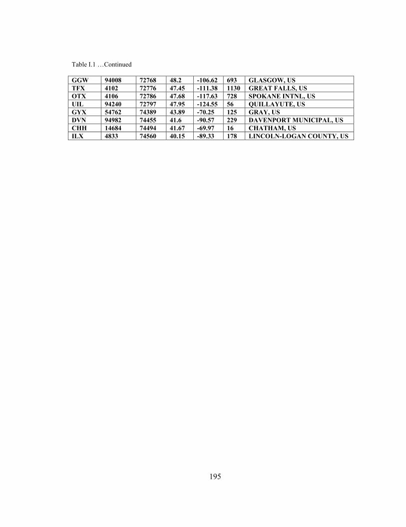
195

Table I.1 …Continued

GGW 94008 72768 48.2 -106.62 693 GLASGOW, US

TFX 4102 72776 47.45 -111.38 1130 GREAT FALLS, US

OTX 4106 72786 47.68 -117.63 728 SPOKANE INTNL, US

UIL 94240 72797 47.95 -124.55 56 QUILLAYUTE, US

GYX 54762 74389 43.89 -70.25 125 GRAY, US

DVN 94982 74455 41.6 -90.57 229 DAVENPORT MUNICIPAL, US

CHH 14684 74494 41.67 -69.97 16 CHATHAM, US

ILX 4833 74560 40.15 -89.33 178 LINCOLN-LOGAN COUNTY, US

196

II. Appendix II: Monthly Plots of Differences between Dual and

Single RAOB Ray Tracing and a Fitted Function

In each of the following figures in the specified month, the upper plot represents the

average differences of dual minus single RAOB ray tracing of slant hydrostatic delay at

3° elevation angle vs. azimuth (dots with error bars) and a fitted model (black curve). The

lower plot (left) is the same as the above one but in polar plot form and without error

bars. Note that the dashed circles inside polar form are representing -3, 0 and +3 cm from

inside toward outside respectively. The lower plot (right) is the same as the above one but

for absolute differences. a and b in the title of each upper plot refer to the fitted function

as: )sin()cos( azbazad ⋅+⋅= .

Figure II.1– Mean and standard deviation of SHD difference and the fitted model for the month of January

2004.

197

Figure II.2– Mean and standard deviation of SHD difference and the fitted model for the month of February

2004.

Figure II.3– Mean and standard deviation of SHD difference and the fitted model for the month of March

2004.

198

Figure II.4– Mean and standard deviation of SHD difference and the fitted model for the month of April

2004.

Figure II.5– Mean and standard deviation of SHD difference and the fitted model for the month of May

2004.

199

Figure II.6– Mean and standard deviation of SHD difference and the fitted model for the month of June

2004.

Figure II.7– Mean and standard deviation of SHD difference and the fitted model for the month of July

2004.

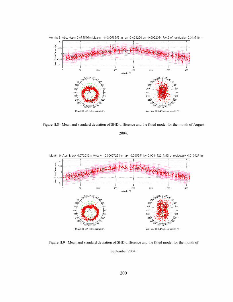
200

Figure II.8– Mean and standard deviation of SHD difference and the fitted model for the month of August

2004.

Figure II.9– Mean and standard deviation of SHD difference and the fitted model for the month of

September 2004.

201


October 2004.

Figure II.11- Mean and standard deviation of SHD difference and the fitted model for the month of

November 2004.

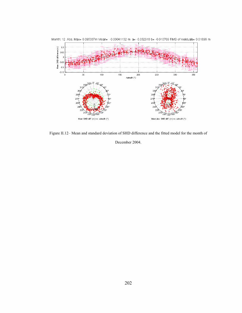
202


December 2004.

203

III. Appendix III: Sample Online-RT Maps

The following are near-real-time maps provided by Online-RT at an arbitrarily chosen

epoch, as examples of the available maps.

Figure III.1- ZWD from global NWP.

204

Figure III.2- ZHD from global NWP.

Figure III.3- Difference between ZWD from global NWP and UNB3m model.

205

Figure III.4- Difference between ZWD from global NWP and UNB3 model.

Figure III.5- Difference between ZTD from global NWP and UNB3m model.

206

Figure III.6- Difference between ZHD from global NWP and UNB3 model.

Figure III.7- Difference between ZHD from regional NWP and UNB3 model.

207

Figure III.8- EW gradient of ZWD from global NWP.

Figure III.9- NS gradient of ZWD from global NWP.

208

Figure III.10- EW gradient of ZHD from global NWP.

Figure III.11- NS gradient of ZHD from global NWP.

209

Figure III.12- Magnitude of ZTD gradient from global NWP.

Figure III.13- Azimuth of ZTD gradient from global NWP.

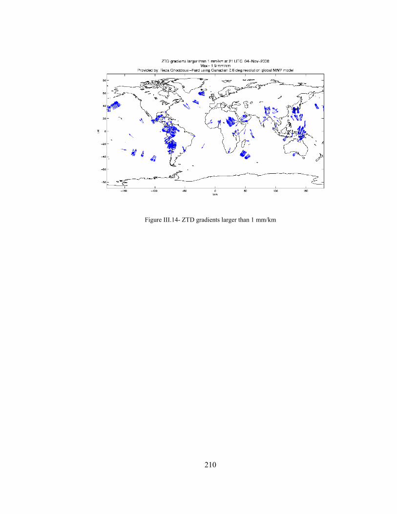
210

Figure III.14- ZTD gradients larger than 1 mm/km

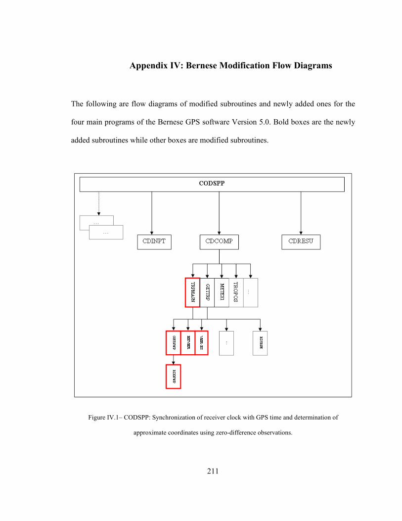
211

IV. Appendix IV: Bernese Modification Flow Diagrams

The following are flow diagrams of modified subroutines and newly added ones for the

four main programs of the Bernese GPS software Version 5.0. Bold boxes are the newly

added subroutines while other boxes are modified subroutines.

Figure IV.1– CODSPP: Synchronization of receiver clock with GPS time and determination of

approximate coordinates using zero-difference observations.

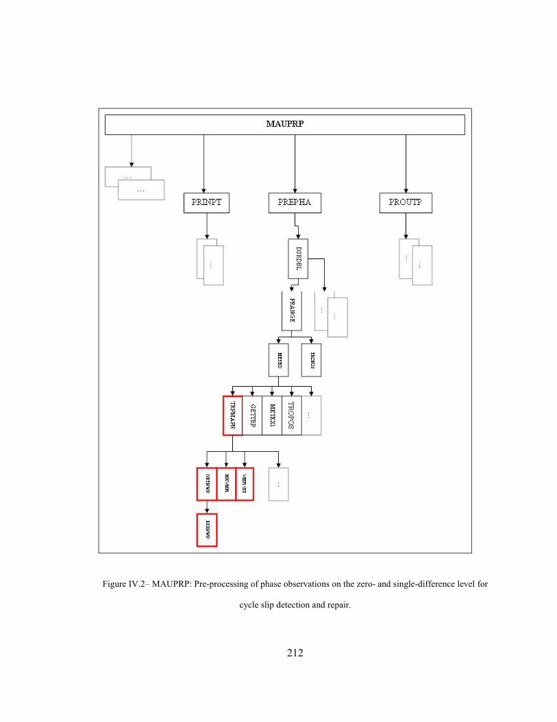
212

Figure IV.2– MAUPRP: Pre-processing of phase observations on the zero- and single-difference level for

cycle slip detection and repair.

I MAUPRP I !

6 . I PRlNPT I PREPHA I PROUI'P

- l "' ~ ~ "' ....

r--

-- -

~ lO :z: Q ,.,

'-r ,..!--- ,..!---

15 8 ~ 'I '-----

• • • • • ~ Q IS: --I

::0 ,., ,., 0 ,.. ~ ~ "" !:!! :s 0 Ul

I ! j_

li.l § I !

'-----

~ ~

'--

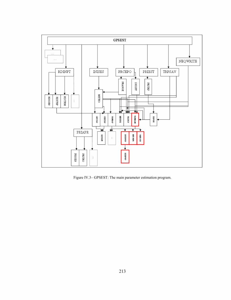
213

Figure IV.3– GPSEST: The main parameter estimation program.

214

Figure IV.4– ADDNEQ2: Combination of results using normal equation files.

215

V. Appendix V: NWP Input File Format Defined for Modified

Bernese

Type: ASCII

Directory: Campaign-specific directory ATM

Extension: NWP

Created by: Ray tracing software

Used by: The file may be introduced in CODSPP, MAUPRP, GPSEST and

ADDNEQ2.

Example: Figure V.1

The NWP file should contain the following information:

1. Title line: Data source and date of run (any text is accepted) 2. Gradient code (1 means file includes gradients, 0 means no gradients) and step

size (in units of day) 3. Data part:

- Station name. - Modified Julian Date. - ZHD (m). - SHD (m). - ZWD (m). - SWD (m). - VEA (rad). - Hydrostatic EW gradient (m). - Hydrostatic NS gradient (m). - Non-hydrostatic EW gradient (m). - Non-hydrostatic NS gradient (m).

216

Figure V

.1- An exam

ple of NWP input file to the m

odified Bernese.

Global 1 dog KWr Q~l --~y tracing run at: 08- Jun- 2008 0.1250

ALGO 54297.000 2. 23220 32 . Hl938 0 . 132108 2 . 181081 0 . 052956 0.000016 -0.000408 0.000066 0.000055 ''NBJ 54297.000 2.283089 33.113076 o . :l9S$6 3 . !><801: 0 . 0$28$6 0 .000408 -0 . 000546 -0.000465 0.000185 liRCl 54291.000 2.262958 32.856516 0 . 139808 2 . 293354 0 . 0!>29!>0 0 .000120 - 0 . 000519 o.ooooeo 0. 000037 At.RT 54297.000 2.295735 33 . 371476 0 . 095571 I. 563332 0 . 053088 -0.000286 0.000192 0.000314 -0.000229 ALGO 54297.125 2.2352~4 32 . 5322~6 0.120313 I. 998074 0 . 052846 -0.000055 -0.000418 0.000109 0.000)09 UNBJ 54291.125 2.283310 33.181013 0 . 233896 3 . 791371 0.052125 0.000445 -0.000597 -0.000659 o.ooouo NRCl 54291.125 2. 266685 32 . ~64699 0 . 133316 2 . 198541 0 . 052838 0 .000090 -0 . 000488 o. 000219 0.000001 ALRT 54291.125 2.295021 33 . 317155 0.089495 l. 465971 0 . 053086 - 0.000309 0.000260 0.000384 -0.000263 At.GO 54297.250 2.2372)4 32 . 560345 0 . 113920 1. 888219 0 . 052851 -0 .000035 -0.000481 -0.0000)2 0.000487 UliBJ 54297. 250 2.283368 33 . 234705 0.228488 3 . 715138 0 . 052613 0.000468 -0.000614 0.0007)5 -0.000653 NRC I 54297 . 250 2. 269047 33 . 017061 0 . 123965 2 . 054584 0 . 052799 0 .000013 -0 . 000551 0. 000118 0 . 000118 ALRT 54297.250 2. 294434 33 . 345589 0 . 086281 1 . 414403 0 . 053090 - 0 .000294 0.000292 0.000279 -0.000250 At.GO 54291. )75 2. 239656 32 . 582921 0.109501 l. 816874 0 . 052885 0 .000002 - 0. 000475 0.000113 0.000526 UNBJ 54297. 3n 2. 284913 33 . 280238 0 . 199098 3 . 252210 0 .05257S 0 .000405 -0.000618 0.001529 -0.001077 NRC I 54291.315 2. 272229 33 . 066519 0 . 116809 1. 940297 0 . 052192 0 .000061 -0.000586 0.000085 0 . 000086 ALRT 54297 . 375 2. 29577~ 33. 365294 0 . 083121 I. 361520 0 . 053085 - 0 .000301 0 . 000344 0 .000245 -0 . 000217 ALGO 54291.500 2.241555 32 . 629696 0 .111893 I. 853939 0 .052841 - 0 .000031 - 0. 000467 -0.000039 0 .000314 UHOJ $4291.500 2.288581 33 . 345104 0 . 131125 2 . 115134 0 . 052551 0 .000321 -0 -000663 -0 .000049 -0.000096 NRCl 54291.500 2.274586 33 . 123878 0 .114781 1.909235 0 .052736 0 .000102 -0 .0005'16 0.000076 -0 .000067 ALRT 54291.500 2. 297090 33 . 399660 0 . 081488 L 335906 0 . 053075 -0 .000279 0 . 000356 0.000071 -0.000074

Curriculum Vitae

Candidate’s full name: Reza Ghoddousi-Fard

Universities attended: B.Sc.E. (Surveying), K.N.Toosi University of Technology, 1995

M.Sc.E. (Geodesy), K.N.Toosi University of Technology, 1999

Publications:

Ghoddousi-Fard R., P. Dare, and R.B. Langley (2008). “Tropospheric Delay Gradients from Numerical Weather Prediction Models: Effects on GPS Estimated Parameters.” Submitted to GPS Solutions. Ghoddousi-Fard R., P. Dare, and R.B. Langley (2008). “A Web-Based Package for Ray Tracing the Neutral atmosphere Radiometric Path Delay.” Computers and Geosciences, In Press, DOI: 10.1016/j.cageo.2008.02.027. Ghoddousi-Fard R. and P. Dare (2007). “A Climatic Based Asymmetric Mapping Function Using a Dual Radiosonde Raytracing Approach.” Proceedings of ION GNSS 2007, 20th International Technical Meeting of the Satellite Division of The Institute of Navigation, Fort Worth, Texas, Sept. 25-28, 2007, pp. 2870-2879. Ghoddousi-Fard R. and P. Dare (2006). “Online GPS Processing Services: An Initial Study.” GPS Solutions, 10: 12-20, DOI: 10.1007/s10291-005-0147-5. Ghoddousi-Fard R. (2006). “Comparison of IGS and Radiosonde Determination of ZTD in the Canadian Arctic.” Proceedings of ION GNSS 2006, 19th International Technical Meeting of the Satellite Division of The Institute of Navigation, Fort Worth, Texas, Sept. 26-29, 2006, pp. 1936-1944. [Student Paper Competition Winner] Ghoddousi-Fard R. and P. Dare (2006). “Comparing Various GNSS Neutral Atmospheric Delay Mitigation Strategies: A High Latitude Experiment.” Proceedings of ION GNSS 2006, 19th International Technical Meeting of the Satellite Division of The Institute of Navigation, Fort Worth, Texas, Sept. 26-29, 2006, pp. 1945-1953. Ghoddousi-Fard R. and P. Dare (2005). “The effectiveness of online GPS processing services.” Proceedings of the 33rd CSCE annual conference, The Canadian Society for Civil Engineering, Toronto, Canada, June 2-4, 2005, pp. GC249-1-10.

Ghoddousi-Fard R. (2002). “Comparison of Terrestrial and GPS Observation Results in a Geodetic Control Network.” Proceedings of the 2nd Symposium on Geodesy for Geotechnical and Structural Engineering, Berlin, Germany, May 21-24, 2002, pp. 515-521. Ghoddousi-Fard R. (1996). “Solving of GPS Carrier Phase Ambiguity.” Proceedings of the 4th Civil Engineering Student Conference, Iran University of Science & Technology, Tehran, Iran, October (In Persian). Conference Presentations: Ghoddousi-Fard R. and P. Dare (2005). “An Investigation on the performance of regional GEM zenith delay products in the Canadian Arctic.” CMOS 2005, Canadian Meteorological and Oceanographic Society, Vancouver, Canada, May. [Abstract published] Ghoddousi-Fard R. (1994). “Applications of GPS in Geomatics.” 2nd Civil Engineering Student Conference, University of Tehran, Tehran, Iran, October. [Abstract published in Persian]

modelling tropospheric gradients and parameters from nwp models… · 2011-11-15 · technical...

Documents