Prepared by the Health and Safety Laboratory for the Health and Safety Executive 2014

Health and Safety Executive

Modelling of liquid hydrogen spills

RR985Research Report

R Batt Health and Safety LaboratoryHarpur HillBuxtonDerbyshire SK17 9JN

In the long term the key to the development of a hydrogen economy is a full infrastructure to support it, which includes means for the delivery and storage of hydrogen at the point of use, eg at hydrogen refuelling stations for vehicles. As an interim measure to allow the development of refuelling stations and rapid implementation of hydrogen distribution to them, liquid hydrogen is considered the most efficient and cost effective means for transport and storage.

The Health and Safety Executive (HSE) have commissioned the Health and Safety Laboratory (HSL) to identify and address issues relating to bulk liquid hydrogen transport and storage and update/develop guidance for such facilities. The second phase of the project involved experiments on unignited (HSE RR986) and ignited releases of liquid hydrogen (HSE RR987) and computational modelling of the unignited releases. This position paper assesses the ability of the cryogenic liquid spill models available to the HSE to model spills of liquid hydrogen by using the new experimental data obtained from the experimental testing at HSL.

A brief literature review on modelling liquid hydrogen pool spread was undertaken and modelling with GASP (Gas Accumulation over Spreading Pools) to compare results with the experimental measurement data. Recommendations are made on improvements to currently available models and also recommendations for further model validation data.

This report and the work it describes were funded by the Health and Safety Executive. Its contents, including any opinions and/or conclusions expressed, are those of the authors alone and do not necessarily reflect HSE policy.

Modelling of liquid hydrogen spills

HSE Books

Health and Safety Executive

© Crown copyright 2014First published 2014

You may reuse this information (not including logos) free of charge in any format or medium, under the terms of the Open Government Licence. To view the licence visit www.nationalarchives.gov.uk/doc/open-government-licence/, write to the Information Policy Team, The National Archives, Kew, London TW9 4DU, or email psi@nationalarchives.gsi.gov.uk.

Some images and illustrations may not be owned by the Crown so cannot be reproduced without permission of the copyright owner. Enquiries should be sent to copyright@hse.gsi.gov.uk.

ii

CONTENTS

1 INTRODUCTION ..................................................................................... 1 1.1 Background.............................................................................................. 1 1.2 Approach ................................................................................................. 1

2 LITERATURE REVIEW ........................................................................... 2 2.1 Models ..................................................................................................... 2 2.2 Liquid hydrogen spill experiments ............................................................ 3 2.3 Physical processes at the source ............................................................ 4

3 TEST 6 MEASUREMENT ANALYSIS .................................................... 7

4 GASP MODELLING APPROACH ......................................................... 12 4.1 Model input and output .......................................................................... 12 4.2 Vaporisation rate validation ................................................................... 13 4.3 Experimental test case – HSL Test 6 ..................................................... 15

5 RESULTS AND DISCUSSION .............................................................. 18 5.1 Vaporisation rate validation ................................................................... 18 5.2 Experimental test case – HSL Test 6 ..................................................... 21

6 CONCLUSIONS .................................................................................... 26

7 RECOMMENDATIONS ......................................................................... 28

8 REFERENCES ...................................................................................... 29

iii

iv

v

EXECUTIVE SUMMARY

Objectives

The objective of this work was to assess the ability of the cryogenic liquid spill models available to the Health and Safety Executive (HSE) to model spills of liquid hydrogen by using the new experimental data of Royle and Willoughby (2012). In order to meet this objective three main tasks were undertaken:

A brief literature review on modelling liquid hydrogen pool spreading.

Carry out modelling with GASP (Gas Accumulation over Spreading Pools) and compare results with the experimental measurement data taking into account issues specific to liquid hydrogen, including sensitivity to specific model parameters or modelling assumptions.

Provide recommendations on improvements that could be made to currently available models and also recommendations for further model validation data.

Main Findings

The literature review showed that most previous modelling of liquid hydrogen spills had been carried out using integral models such as GASP, which is the model currently used by HSE for modelling pool spreading. There has been relatively little three dimensional Computational Fluid Dynamics (CFD) modelling carried out to date, the majority of which has used a simpler model to provide source information and CFD to model the subsequent gas dispersion. However, there have been recent developments in CFD modelling of the pool spreading itself, along with other source options.

An analysis was carried out of the measurements from the ground level probes used in Test 6 of the experiments undertaken at HSL (Royle and Willoughby, 2012). This analysis showed evidence of a gravity current of cold air that propagated ahead of the spreading pool of liquid hydrogen. The radius of the spreading pool was extracted from the Test 6 experimental data for comparison with the GASP model. The setup configuration of Test 6 means it is the most suitable of the HSL experimental datasets for validation of the model. The extracted data showed a pool increasing rapidly to a fairly constant radius, expanding further and then retracting. Once the release stopped the pool showed potential preferential evaporation from the centre.

Two validation exercises were carried out using GASP. A preliminary validation was performed of the vaporisation rates for contained, non-spreading, liquid oxygen and liquid hydrogen on a concrete substrate using published experimental data. However, uncertainty in the thermal properties of the concrete in the experiment made the validation exercise difficult. Some differences in the experimental results and model predictions were observed, one possible explanation being film boiling occurred in the hydrogen tests, which GASP does not account for. It was also shown that GASP can produce spurious results if the wind speed is set to zero, although in cases where boiling dominates the liquid vaporisation, as in the cases considered here, reasonable results can be obtain by setting a low wind speed of, say, 0.1 ms-1.

The second validation exercise was performed against the HSL Test 6 results. The model predictions of the time to vaporisation after the release had stopped were found to be sensitive to the so-called ‘puddle depth’. Overall, GASP performed better than expected and provided predictions of the pool radius that were in reasonable agreement with the experimental data despite the model not being able to account for the solid formation seen in the experiments. The hydrogen vaporisation rate was not measured in the experiments so validation of this parameter

vi

was not possible, however, the predicted mean vaporisation rate was found to be equal to the discharge rate and was not sensitive to the modelling parameters.

To better understand the capabilities of GASP for modelling liquid hydrogen pool spreading further validation is needed in the areas of heat transfer, pool spreading and vaporisation. Only then could it be recommended as a reliable model for liquid hydrogen spills.

1

1 INTRODUCTION

1.1 BACKGROUND The lack of suitable experimental measurements for validating cryogenic liquid spill models is frequently raised (Hissong, 2007, Middha et al., 2010, Venestanos et al., 2010). Many previous modelling studies have relied on measurements from experiments with LNG to validate their models for liquid hydrogen. HSL recently produced a state of the art review on modelling liquefied natural gas (LNG) source terms for hazard analysis (Webber et al., 2010). The physics of LNG spills on land are described by Webber et al. (2010) and many of these physical processes are also relevant to liquid hydrogen spills. However, with few measurements and observations available and temperatures significantly lower than for LNG, the validity of this assumption may not always be appropriate.

Two international research initiatives that have previously dedicated a significant amount of work to modelling hydrogen are Hysafe1 and WE-NET2. However, there are few studies that attempt to measure the processes involved in a liquid hydrogen spill, rather than solely focus on hydrogen dispersion and explosions, including its interaction with ambient conditions and obstacles. As a result of this there remains a general lack of understanding that is necessary for accurate modelling. In particular, processes at the source have usually not been captured adequately for modelling and so source characterisation is often very difficult. A poorly characterised source will not result in accurate dispersion modelling (Gavelli et al., 2009).

Recently, HSL has undertaken a series of experimental tests releasing liquid hydrogen on a concrete pad at their test site in Buxton. The measurements and results of these tests are presented in detail by Royle and Willoughby (2012) and Hall, Willoughby and Hooker (2013) for unignited and ignited releases, respectively. These tests provide valuable data on the spreading of liquid hydrogen pools and the subsequent hydrogen dispersion. The measurements are sufficiently well-defined for the validation of pool models.

1.2 APPROACH

A review of models for liquid hydrogen pool spreading and vaporisation has been carried out. This is supplemented by a summary of the physics of pool spreading and vaporisation. These reviews allow the issues specific to liquid hydrogen to be established and potential parametric and modelling sensitivities to be identified.

The liquid hydrogen spill experiments of Royle and Willoughby (2012) have been analysed from which information on the pool radius was extracted and the pool spreading phenomena was analysed. This analysis was designed not only to provide model validation data but also to give insight into the spreading liquid pool dynamics.

Computational modelling was carried out using GASP (Gas Accumulation over Spreading Pools), as used by HSE for cryogenic liquid spills. The approach to validation was then in two stages such that the first stage could provide validation of the vaporisation submodels, without the spreading and the second stage would attempt to model Test 6 from the experimental test series of Royle and Willoughby (2012), including sensitivity studies of certain parameters. Following on from the model validation, additional information that could be output by GASP but was not available from the experiments was evaluated.

Recommendations for further model validation data have been made in this report in addition to recommendations on improvements that could be made to currently available models. 1 http://www.hysafe.org/ accessed on 26/09/11 2 http://www.enaa.or.jp/WE-NET/ accessed on 26/09/11

2

2 LITERATURE REVIEW

2.1 MODELS

The modelling of liquid hydrogen spills is usually carried out in two parts: firstly the liquid spread and vaporisation is modelled and then the output of this model is used as an input, or source term, to a dispersion model of the hydrogen gas / vapour. The initial liquid spread and vaporisation phase involves processes occurring in shorter time scales compared to the dispersion phase, therefore it is very difficult for one model to be able to represent both phases of the release. For this reason, numerical models are typically split into source term models, which account for the release details and gas dispersion models with input taken from the former. This approach relies heavily on the source term model providing accurate input information and so a significant amount of work concentrates on this aspect, including the present study.

Liquid hydrogen spill models can be broadly categorised into three approaches; integral, shallow layer and CFD. The only approach that is potentially able to cope with modelling the entire process is a CFD model, but although evaporation can be included in many CFD models, modelling of additional complex processes such as boiling may not yet be sufficiently advanced for this application. Furthermore, even with modern processing power the complexity involved is still likely to result in significant computing cost.

Integral models involve the solution of ordinary differential equations which describe the integral properties of the pool. This typically means modelling the rate of increase of the pool radius with time with the assumption that the pool is circular and the depth of the pool is an average calculated over the pool area. As a result, one of the limitations of these models is that they cannot cope with complex terrain, however, simple topographical features such as surface roughness, puddles and bunds can be modelled. GASP (Webber, 1990, see section 4) is an integral model and is currently used by HSE for modelling liquid spills and has been well validated and used for modelling LNG releases, for example, but has not been validated for liquid hydrogen spills. The work of Brambilla and Manca (2009) uses GASP and adopts physical sub-models from previous work to create a more advanced model. The modifications include a friction term in the presence of film boiling; friction velocity; wind profile index; conductive heat flux; radius-time dependence at the pool minimum thickness; and turbulent mixing onto water. GASP can be used to automatically generate input files for the dispersion model DRIFT (Webber et al., 1992a,b).

An approach of intermediate complexity between CFD and integral models is to model the pool spread using the shallow layer equations. These are a system of two-dimensional partial differential equations and are therefore more complex to solve than integral models but they do not seek to solve the fully three-dimensional turbulent flow equations of more general CFD approaches. Shallow layer models have been used extensively in one and two layer forms to model releases of non-volatile fluids and exchange flows, for instance, the LAuV (Lachen-Ausbreitung-und-Verdampfung) shallow layer model of Verfondern and Dienhart (1997, 2007) has been used to model liquid hydrogen spills. This is a proprietary code developed at Forschungszentrum Julich. The work that led to the development of this model is to date one of the most comprehensive experimental and numerical studies on the spreading of cryogenic liquid pools. The model is one dimensional, axi-symmetric and can simulate releases onto the ground or water and includes a sub-model for ice formation and has also been validated against LNG and liquid nitrogen spill tests. At present the LAuV code is no longer in use (Jäkel, 2011).

There is a relatively small amount of CFD modelling that has been performed on releases of liquid hydrogen; the most prolific work has been performed using the codes CHAMPAGNE

3

(Morii and Ogawa, 1996), ADREA-HF (Statharas et al., 2000) and FLACS (FLACS, 2010). The general purpose CFD codes FLUENT and CFX have also been used (Schmidt et al., 1999, Molkov et al., 2005, Sklavounos and Rigas, 2005). All of these studies use the Reynolds Averaged Navier Stokes (RANS) equations except Molkov et al. (2005) who use a large eddy simulation (LES).

2.2 LIQUID HYDROGEN SPILL EXPERIMENTS To date experiments on liquid hydrogen spills having only included qualitative observations, which are of limited use for validating models. Typically, experiments have included little quantitative measurement or insufficient detail in the experimental documentation to model the source physics accurately. A brief summary of several hydrogen spill experiments can be found in Venetsanos et al. (2010). The most frequently used experimental datasets for validation of liquid hydrogen spills are the BAM (Marinescu-Pasoi and Sturm, 1994) and NASA (Chirivella and Witcofski, 1986) trials. Both require significant assumptions and estimations to be made when modelling the experiments due to uncertainties in the source release mechanisms.

Of the above CFD models ADREA-HF (Statharas et al., 2000), FLACS (Arntzen and Middha, 2008) and FLUENT (Schmidt et al, 1999) have all been used to simulate the BAM experiments. The following have also made comparisons with the NASA data: Chitose et al. (1996) - CHAMPAGNE, Venestanos and Bartzis (2007) - ADREA-HF, Middha et al. (2010) - FLACS, Molkov et al. (2005) - FLUENT and Sklavounos and Rigas (2005) - CFX. Most of these studies concentrate on modelling the hydrogen dispersion due to a lack of measurements within the liquid pools that formed during the tests. These limitations have led several studies to calibrate their models by varying the source methods to assess which gives the best fit to the measurements (e.g. Venestanos and Bartzis, 2007).

As mentioned previously, the characterisation of the source, for example as a jet or a pool is very important and has significant impact on the subsequent gas dispersion. Venestanos and Bartzis (2007) discuss this and Schmidt et al. (1999) acknowledge that the lack of good agreement between their results and the measurements is in part due to their modelling the release solely as gas. The models CHAMPAGNE, ADREA-HF and FLACS all have the capability to model a liquid phase as a source. For example, for the NASA case, in ADREA-HF the source pool is modelled as either a fixed radius upward pointing inlet of 100% gas on the bottom boundary or a downward pointing two-phase jet with and without a fence representing the bounding wall of the pool (Venestanos and Bartzis, 2007). Sklavounos and Rigas (2005) model the pool in CFX with a fixed radius, upward pointing inlet of 100% gas set in a recess to represent the bounding wall. They find similar agreement to the experimental data with their model as Venetsanos and Bartzis (2007) do with their jet model despite the fact that the latter reject the use of the 100% gas inlet in favour of the jet due to its poor agreement with the experimental measurements.

For the same test CHAMPAGNE applies a split inlet boundary on the left wall of the domain (2D). This means that at the bottom cell of the inlet the fluid is specified as liquid hydrogen while nitrogen is specified on the remainder of the inlet above this cell (Chitose, et al., 1996). FLACS uses a more sophisticated approach to modelling the hydrogen source by using an embedded shallow-layer model to simulate the pool spread (Hansen et al., 2007). Chitose et al., (1996) found that the mass flux evaporated strongly influenced the subsequent vapour dispersion and attempted to modify the CHAMPAGNE code to account for this (Chitose et al., 2002b). The Molkov et al. (2005) FLUENT model used hydrogen gas at 20.4 K as the source with two different gas ‘pools’, one fixed and one of increasing size. Unfortunately, they also modify the mesh and boundary conditions in each of these cases so it is difficult to conclude which is the more valid approach. Overall, they conclude that the results are dependent on both initial and boundary conditions.

4

2.3 PHYSICAL PROCESSES AT THE SOURCE

In order to generate an accurate source model the physical processes that occur in pool spread and vaporisation must be identified and represented in the model. Verfondern and Dienhart (2007) summarise many observations of liquid hydrogen releases on water and on land. The typical behaviour of a cryogenic liquid release is that as the surface area of the pool increases the vaporisation rate also increases such that eventually an equilibrium state is reached where the liquid spill rate balances the vaporisation rate. It should be noted that this equilibrium state may only exist in some time averaged form, i.e. there may be some oscillations about the equilibrium. In some cases GASP predicts that the pool should expand well beyond the equilibrium radius and evaporate completely while the source is still providing liquid. This would suggest that the equilibrium is not stable – or at least that the system is underdamped if the initial spread rate is rapid enough.

On solid ground the surface in contact with the cryogenic liquid is cooled which results in a decrease in heat transfer from the ground to the liquid and so spreading can continue. Hence, even though a pseudo-equilibrium state has been reached, the surface area of the pool does not necessarily remain constant. If the release is confined by a bund for example, the surface area cannot increase and the vaporisation rate will reduce.

The only study to date to compare releases of several cryogenic liquids under identical conditions is the theoretical study of Verfondern and Dienhart (2007) using the LAuV code. The study compared the spreading behaviour of liquid oxygen, liquid hydrogen, LNG and liquid nitrogen on macadam. The liquid hydrogen pool was predicted to be both smaller and shorter lived than the other releases. For example, for a continuous release of liquid hydrogen, the pool was predicted to have completely vaporised by 5 seconds whereas for a LNG release complete vaporisation took over 55 seconds. Liquid hydrogen is significantly colder at typical storage conditions than other cryogenic liquids, with a boiling point of 20.4 K compared to 111.4 K for liquid methane. Liquid hydrogen also has a boiling point well below that of oxygen (90 K) and nitrogen (77 K) and therefore a liquid hydrogen spill could be expected to condense the surrounding air. The heat released if these gases condense would then supply an extra heat flux into the pool and potentially enhance the vaporisation rate of the hydrogen.

Verfondern and Dienhart (2007) note that in both NASA and BAM experiments of hydrogen spills on water the pool area was observed to ‘pulsate’, meaning that the pool radius alternated between expansion and retraction. Furthermore, on an aluminium sheet in the BAM experiments a difference in radius between 0.3 - 0.5 m for a release rate of 6 litres per second was observed. The liquid spill on to solid ground also led to the pool fracturing into pieces resulting in ice floes. Verfondern and Dienhart (2007) state that the very low kinematic viscosity of hydrogen was influential in determining the stability of the pool front, its break up and the pulsation behaviour of the pool. In terms of a general cryogenic liquid pool spreading, Verfondern and Dienhart (2007) note that the pool retracts once the release has stopped and that when the depth of the cryogenic liquid pool reduces below a minimum defined by the surface tension of that particular cryogen, the pool breaks up into floe-like islands.

The boiling of cryogenic liquid spills, including liquid hydrogen, can be described by three very different boiling regimes. Film boiling is characterised by a vapour film forming between the cold liquid and the warmer surface. Chitose et al. (2002a) found that in this phase the spreading liquid hydrogen broke up into small spherical droplets and spread by rolling across the top of the vapour. They suggest that a model might over-estimate the evaporation rate for liquid hydrogen in the early stages if it does not account for the reduced contact area of the rolling droplets compared to a continuous liquid pool. Chitose et al. (2002a,b) modified the CHAMPAGNE model to account for this. Interestingly, when they applied the model to liquid

5

nitrogen it overestimated the liquid spreading rate, since the droplet phase did not occur for this substance. Instead, the liquid spread as a pool on top of the vapour film.

In the model GASP, Webber and Jones (1989) assume that film boiling does not take place for pools on solid surfaces. They cite the work of Moorhouse and Carpenter (1986), which suggests that film boiling can only occur on an unheated surface if it is a highly conductive, uncoated metal surface, which are unlikely to be found in practical applications.

The second characteristic boiling regime is that of transition boiling where the vapour film collapses and gives way to the third regime of nucleate boiling where the liquid is in direct contact with the surface. This regime is also called the steady phase and the rolling spread of the liquid on a vapour film disappears.

An increase in ground porosity and ground materials of higher water content were found to increase boil off rates of LNG (Webber et al., 2010). Verfondern and Dienhart (2007) discuss differences in the vaporisation of a cryogenic liquid for wet and dry concrete and observe that the vaporisation rate on the wet surface decreases compared to the dry case due to insulation effects. However, if a 3 mm layer of surface water is present on top of the wet concrete the vaporisation rate increases compared to the wet case with no surface water since the water layer freezes and acts as an insulating layer. Despite this insulation, the vaporisation is still faster than the dry case. For liquid hydrogen, Takeno et al. (1994) concluded that the evaporation mechanism was identical for wet and dry sand and postulate that this is due to water freezing in the cavities between sand particles in the former case and freezing air in the latter case due to the very low temperatures encountered with liquid hydrogen. Takeno et al. (1994) find that the variation of vaporisation rates with time was approximately proportional to t—1/2 (in accord with simple theories where conduction in a uniform substrate dominates the heat transfer) for both of the substrate materials used, except in the early stages just after release. For comparison, the evaporation rate of liquid oxygen on the dry sand was approximately constant. They suggest that this is because the boiling point of liquid oxygen, unlike that of liquid hydrogen, is not low enough to freeze the air in the cavities and so the liquid soaks into the dry sand while vaporising. The vaporisation rate was therefore proportional to the downward velocity of the liquid through the sand.

Atmospheric conditions also have an effect on the vaporisation of liquid hydrogen spills; the condensation of air and subsequent additional heat flux has been mentioned previously. None of the models discussed here include this contribution to the heat flux, and so, by applying them, one is making the implicit assumption that condensation of oxygen and nitrogen, if it happens, makes only a small contribution to the heat flux. Certainly, for liquid hydrogen spills the ground temperature has been shown to be more important than the atmospheric convection and radiation in terms of heat input, with 80-90% of the heat flux to the pool originating from the ground (Verfondern and Dienhart, 2007). Despite this, Molkov et al. (2005) suggest that the increased heat flux could lead to positive buoyancy in the hydrogen gas / vapour and including the condensation of air above the pool in their modelling may improve the agreement with the NASA experimental results. By contrast, Middha et al. (2010) have also discussed this and, interestingly, they suggest that condensation of air would increase the density of the cloud providing negative buoyancy due to the presence of a particulate phase. Ground roughness is also likely to be important, directly affecting the spread of the liquid and also vaporisation (away from the boiling regime) through effects on the wind profile.

Few modelling studies account for the air humidity. In the case of the NASA experiments this may not have too much impact since they were performed in the desert. In other locations this factor could have a significant effect on the heat available for vaporisation of the liquid. Giannissi et al. (2011) have used ADREA-HF to model some of the experiments of Royle and

6

Willoughby (2012) including an assessment on the development of the cloud when humidity is ignored in the model. They found that when humidity was included, the model showed significantly better agreement with the concentration data than when it was neglected. They conclude that this is due to increased positive buoyancy. The implication of this is that when humidity is present the flammable region of the cloud does not extend so far down wind compared to when humidity is neglected.

7

3 TEST 6 MEASUREMENT ANALYSIS

Of the liquid hydrogen spill trials performed by Royle and Willoughby (2012), Test 6 is the most suitable experimental dataset for validation of the GASP model since the release nozzle is orientated vertically downwards 10 mm above the ground. This configuration is most likely to be approximated by a radial spread as assumed by the model. Full details of the experimental measurement setup, procedure and results can be found in Royle and Willoughby (2012). A brief description of the probe locations is given here for reference.

The measurement probe setup is shown in Figure 1. There were 24 ground level thermocouples mounted in a horizontal line spaced 100 mm apart starting at a distance of 500 mm from the source, i.e. from 0.5 m to 2.8 m. The tips of the thermocouples were in contact with the surface of the concrete substrate. There were 3 thermocouples embedded in the concrete at depths of 10 mm, 20 mm and 30 mm to measure the substrate temperature. Finally, there were 30 concentration sensors arranged at 5 points in a horizontal line in line with the wind direction in vertical arrays of 6, see Table 1.

Figure 1 Probe layout used in experimental measurements of Test 6 (Royle and

Willoughby, 2012)

Table 1 Locations of 30 concentration probes Horizontal distance from release (m) 1.5, 3.0, 4.5, 6.0, 7.5 Vertical locations at each horizontal location (m) 0.25, 0.75, 1.25, 1.75, 2.25, 2.75

8

A key parameter in validating the GASP model is the spreading rate of the pool and hence the radius of the pool as a function of time. This was not directly measured during the experiments and therefore had to be extracted from the ground level probe data. Given the boiling point of hydrogen of 20.4 K, it was assumed that if the probe temperature fell below 30 K then that probe was within the liquid pool. A similar analysis carried out by Chitose et al. (2002a) used a value of 50 K to define the boundary of the pool. A quick check on the current data showed that the pool radius was not sensitive to the value used to detect the boundary of the pool.

The radius of the pool extracted from the Test 6 measurements is shown in Figure 2. The pool can be seen to rapidly expand to between 0.9 m and 1.0 m and remain at this size for nearly 200s. It then expands rapidly again to between 1.3 m and 1.4 m and remains at this size for a short period of time before retracting. The pool radius then returns to between 0.9 m and 1.0 m, remaining at this size until the discharge stops. It is possible that the stop in spreading and then sudden further expansion is caused by solid deposition on the ground, which suddenly breaks down allowing further liquid spread. Departure from a smoothly varying pool radius is not unexpected, as ‘pulsating’ pools have been observed previously by Verfondern and Dienhart (2007).

Figure 2 Radius of the pool extracted from experimental measurements showing

expansion and retraction

Once the release stopped, it took 16.9 s before the first ground level probe, 0.5 m from the source, indicated that it was no longer in the liquid pool. Figure 2 shows that the pool does not necessarily vaporise from the outside inwards as the probes 1 to 5 indicate that the temperature rises above 30 K at about the same time. In fact, if 50 K were used as the maximum pool temperature the pool would be observed to vaporise from the inside outwards. Without further information, it was assumed that the time for total pool vaporisation after release stops was approximately 17 s.

The temperature data of the ground level probes (see Figure 1) from which the radius was derived is shown in Figure 3. A quick view of the results highlights the times at which the

0

0.2

0.4

0.6

0.8

1

1.2

1.4

0 100 200 300 400 500 600

Time (s)

Poo

l rad

ius

(m)

Release stop

Radius (m)

RETRACTION EXPANSION

9

various probes are in the pool, where the temperature drops to around the boiling point of hydrogen, and that choice of the criterion for defining the edge of the pool is not critical as long as it is somewhere in the range between the boiling point of hydrogen and below the boiling point of nitrogen (77K).

The liquid pool radius can be seen to be at its largest at around 200 s where probes 1 to 8, and possibly 9, lie within the liquid pool. Probes 10 – 24 are not shown in Figure 3 since the temperatures do not drop below 30 K and are therefore are not considered to lie within the pool for the duration of the release. The temperatures measured by these more distant probes lie approximately between 100 K and 250 K with the value increasing with distance from the source. It is also clear in Figure 3 when the temperature of the probes rise above the boiling point of hydrogen at which point it is assumed that the pool has vaporised.

Figure 3 Temperature measurements from Test 6 probes 1 – 9.

In Figure 3 the probes 6 – 9 exhibit interesting behaviour, most notably before the pool reaches them. The measured values are near the boiling points of oxygen (90.2 K) and nitrogen (77.4 K), the largest components of air. This distinct increase from the boiling point of hydrogen to approximately that of air can also be observed once the release has stopped in the BAM experiments (see Figure 3 in Statharas et al., 2000). The following analysis indicates that this is consistent with a downward dense plume of cold air over the pool, being deflected at the ground into a radially spreading cold gravity current. This phenomenon is simplified in the diagram in Figure 4, which is also used for reference.

0.0

50.0

100.0

150.0

200.0

250.0

300.0

0 100 200 300 400 500 600 700 800 900

Time (s)

Tem

pera

ture

(K)

Probe 1Probe 2Probe 3Probe 4Probe 5Probe 6Probe 7Probe 8Probe 9Release stop

O2 BP ~90 K N2 BP ~77 K

Pool vaporised

H2 BP ~20 K

10

P – Plume of cold air descending G – Radially spreading cold air gravity current C – Cold air transition zone

Figure 4 Diagram of downward dense plume of cold air over the pool.

Assuming a quasi-steady flow is set up, the air in zone C in Figure 4 can cool to ~90 K at which point any further heat removal will condense O2, making this a limiting lower value. The ambient air temperature is 283 K and so the air in zone C is approximately 3 times as dense as the ambient air. This density difference determines the buoyancy forces.

The velocity scale in the plume, P in Figure 4, is given by

0RgKuP ′= ( 1 )

Where K = O(1) and depends on the heat transfer rate from the air to the pool and R0 is the radius of the pool shown in Figure 4. The reduced gravity, g′ is given by ( ) aag ρρρ /− where g is gravitational acceleration, ρa is the density of the ambient air and ρ that of the dense plume.

The radial velocity is uR such that

PR uRuHR 20002 ππ = ( 2 )

Where H0 is the depth of the radially spreading cold gravity current shown in Figure 4. If it is assumed that uP ~ uR in equation ( 2 ) then H0 ~ R0 / 2.

For the process in Figure 4 to approximate the temperature measurements shown in Figure 3 the cold gravity current must spread faster than the pool, i.e.

dtdRRgK 0

0 >′ ( 3 )

It was observed for Figure 2 and Figure 3 that for about 200 s the radius of the pool remains approximately constant at R0 ~ 1.0 m. If K = 1 then 5.4~0Rg′ ms-1. Therefore, equation ( 3 ) holds and the cold cloud readily spreads beyond the pool.

R0

H0

P

G G C

Pool of liquid H2 of fixed size

Calm air Calm air

uR

uP

11

The above analysis implies that if H0 ~ R0 / 2 and R0 ~ 1.0 m for the first 200 s then the depth of the current is approximately 0.5 m. The nearest experimental measurement point in the ambient air (or cold cloud) above the pool was at 1.5 m with the nearest probe in the array 0.25 m away from the ground. The average temperature within the first 200 s at this distance from the source in the cloud and at ground level was extracted from the data and is shown in Figure 5. It can be seen that at this distance from the source and with a liquid pool of approximately 1.0 m there is a cold layer near the ground outside of the pool. The temperature profile shows that an approximate estimated cloud depth of 0.5 m is consistent with the temperature measurements.

Figure 5 Temperature measurements averaged over the first 200 s after release for

the array of cloud probes and the ground probe at 1.5 m from the source.

0

1

2

3

0 50 100 150 200 250 300

Temp (K)

Hei

ght (

m)

Probe array, 1.5 mAmbient airH0 ~ 0.5 m

12

4 GASP MODELLING APPROACH

GASP was developed by ESR Technology for modelling the spread of pools from hazardous spills and includes processes appropriate for modelling cryogenic liquids such as heat transfer and vaporisation. It is one of HSE’s approved models for this type of release. Version 4.0.2 of the GASP model has been used for all of the calculations reported here.

The software solves ordinary differential equations for the integral properties of the pool including modelling the rate of increase of the pool radius with time. GASP assumes spreading due to gravity only and the pool is assumed to be circular and remain so as it spreads; the depth of the pool is an average calculated over the pool area. Processes that are required by the model, such as vaporisation, are incorporated into the equations through sub-models. It is important to note that GASP was developed at a time (the mid-1980s) when liquid hydrogen was not among the substances of greatest concern, and GASP does not include the possibility of oxygen or nitrogen condensing from the air. Applying it to the current problem therefore involves the assumption that any such condensation is not a major contributor to the behaviour of liquid hydrogen pool spreading and vaporisation.

A full description of the mathematical derivation of the model and its implementation in the code is provided by Webber (1990).

4.1 MODEL INPUT AND OUTPUT

GASP can calculate both instantaneous and continuous releases onto water and solid ground. A continuous spill can be defined by a combination of aperture size, flow rate and velocity and limited by volume or duration. The roughness of the liquid pool surface can be specified and this has an effect on the wind profile, which in turn affects the vaporisation rate, though this effect should be negligible for boiling pools.

GASP provides two methods by which a pool can have a finite depth without spreading. These are based on a capillary depth or a ‘puddle’ depth. The capillary depth is the pool depth at which the surface tension balances the gravitational force that is trying to cause the pool to spread further (Webber and Jones, 1989) and is the mechanism by which droplets of finite depth can remain on a smooth surface. This option allows for the effects of surface tension in limiting the spread of the pool by setting the frontal depth of the fluid to a constant value3. This is the only way in which the surface tension affects the pool spreading in GASP (Webber, 1990). The concept behind specifying a puddle depth is based on the assumption that the land over which the pool spreads is sufficiently uneven that puddles can be formed, and this will determine the maximum area that the pool will cover (Webber and Jones, 1989). Two layers of liquid are distinguished in the theory, a dynamic flowing layer and a stagnant layer that lies in puddles within depressions in the ground (Webber, 1990). The mean depth of these puddles, averaged over the entire land surface is the puddle depth specified by the user. The model removes mass and momentum from the pool as it spreads over the depressions. The capillary depth is only used for modelling pool spread over water (or in theory any other liquid substrate) and the puddle depth is only used for liquid spread over solid terrain.

The model can output various parameters for validation purposes and to supplement the experimental measurements. For example, pool radius, depth, vaporisation rate and calculation

3 It should be noted that real world situations (such as droplets on a window pane) where a non-zero depth is maintained by surface tension, are usually possible only if the surface is clean. This may therefore not always be a useful mechanism to represent industrial situations.

13

of the time for the pool to evaporate after the release stops. The output is in an easy to use tabular format.

4.2 VAPORISATION RATE VALIDATION

A review of GASP validation studies relevant to spills of LNG is provided by Webber et al. (2010), but no previous validation studies have been carried out for liquid hydrogen. A preliminary validation test was performed on the vaporisation rates of non-spreading pools of liquid hydrogen and liquid oxygen using the data of Takeno et al. (1994). The mass vaporised and heat flux to a liquid hydrogen and liquid oxygen pool was measured by Takeno et al. (1994) with the pool on an infinitely deep sand or concrete substrate. Twelve tests were performed with liquid volumes of 0.0005 – 0.002 m3 in vessels of diameter 0.05 m and 0.1 m. The results for the concrete case were used to provide data for validation for this study. It was not possible to make a direct comparison with the measurement data as access to the original data was not available and the paper does not state which of the sets of measurement conditions the results presented represent. The conditions input into GASP are summarised in Table 2.

Table 2 Input into GASP for Takeno et al. (1994) validation cases Liquid hydrogen Liquid oxygen Substrate Concrete Concrete Heat transfer Perfect thermal contact Perfect thermal contact Bund radius (m) 0.05 0.05 Release type Instantaneous Instantaneous Substance Hydrogen Oxygen Pool Radius 0.05 0.05 Pool roughness (m) 0 0 Depth (m) 0.127 0.255 Initial pool temperature (K) 19 89 Ambient temperature (K) 288.15 288.15 Wind speed (ms-1) 0.1 0.1 Surface roughness (m) 0 0

Takeno et al. (1994) also compare their experimental results with an analytical result for the variation in the heat flux, q(t), from the surface of the concrete to the liquid. This is derived from the one-dimensional unsteady-state thermal conduction equation in the concrete layer, with perfect thermal contact between the concrete and the liquid, and is given by

( ) ( )

( )( ) 2/10

0/−

=

−=

−=

tTT

dzdTtq

sLs

zss

παλ

λ

( 4 )

where λs and αs are the thermal conductivity and diffusivity of concrete, respectively. In our analysis4, the values were set to the default values for concrete used in GASP of λs = 0.93 Wm-1K-1 and αs = 4.8 × 10-7 m2s-1. The vertical distance below the concrete surface is denoted by z; TS, T0 and TL are respectively the temperature within the concrete layer, the initial temperature of the concrete and the temperature of the top surface of the concrete (assumed to remain constant at the boiling point of the liquid).

4 Takeno et al (1994) report using ‘known values’ of conductivity and diffusivity but they do not provide the values used or information on how they obtained them.

14

Takeno et al (1994) observe the classic t-1/2 behaviour in the mass vaporisation after 2 to 5 seconds, and quote the pouring time as 1 to 2 seconds. It therefore appears that a heat flux of the form ( 4 ) is established as soon as one might reasonably expect.

The experiments of Takeno et al. (1994) are a ‘difficult’ case for GASP as in one respect they do not resemble the normal hazard scenario for which GASP was designed: the experiments were in a deep glass vessel, precluding any air flow over the liquid surface. This means that GASP’s vaporisation model cannot strictly apply.

GASP’s thermodynamics are sketched in Figure 6 below. Consider a steady rate of heat input (shown by the horizontal line) into a pool well below its boiling point, TB. The temperature will increase while the heat input is greater than that taken out by the heat of vaporisation (shown by the lower curves). This will continue (moving to the right on the graph), until a heat balance is achieved (where the heat input and heat of vaporisation lines cross). The lower curves show the heat supplied to vaporise the liquid for two different wind speeds: in GASP’s idealised model these tend to infinity at the boiling point. In the case shown in Figure 6 the steady state is achieved very close to (for most intents and purposes, at) the boiling point. This is GASP’s model of boiling. A slightly higher heat input would mean a greater vaporisation rate at equilibrium which would be (infinitesimally) closer to the theoretical boiling point. Therefore, in the boiling régime, the vaporisation rate is controlled by the heat input, and the temperature is essentially unaffected, and, as illustrated in Figure 6, the boiling rate is completely insensitive to wind speed (and other features of the wind profile such as the aerodynamic roughness length).

Well below the boiling point, far to the left of the graph in Figure 6, the vaporisation rate is sensitive to wind speed (and profile). In the case illustrated, with a high heat input the temperature will increase (by contrast, in the case of blowing across a patch of ether at ambient temperature, the heat input is below the vaporisation heat and the ether cools.)

The idealised model in GASP is not theoretically applicable at zero wind speed: the vaporisation rate is at zero for T < TB and becomes infinite at T = TB, a situation unsuited to the derivation of numerical solutions as boiling is approached. This singularity must be avoided by introducing a small wind speed. As shown in Figure 6, the results for boiling pools will not be sensitive to this as long as this wind speed is fairly low, but it must be high enough to steer well clear of the zero-wind singularity in GASP’s heat exchange model.

15

Figure 6 Heat input and heat of vaporisation against temperature, T. TB is the boiling point of the liquid. The equilibrium where the lines cross represents a boiling pool.

Simpler boiling models define the vaporisation rate by the ratio of heat input and heat of vaporisation. GASP has a complete model capable of modelling both slow vaporisation and boiling and (as illustrated here) transitions between the two, but its disadvantage is the singularity at zero wind speed.

In the experiments of Takeno et al (1994), the gas must escape by spilling over the rim of the vessel, and again the vaporisation rate is expected to be insensitive to how rapidly it escapes. In order to model this phenomenon, we need to substitute this removal mechanism with one represented in GASP, and introduce a small non-zero wind (see Table 2).

4.3 EXPERIMENTAL TEST CASE – HSL TEST 6

GASP was used to model the liquid hydrogen spill, Test 6, carried out by Royle and Willoughby (2012). The GASP model parameters that were used are shown in Table 3.

Table 3 General input into GASP for Test 6. Substrate Concrete Heat transfer Perfect thermal contact Puddle depth (mm) 0.9, 2.6, 5.0 Release type Continuous Pool roughness (mm) 0, 0.5 Substance Hydrogen Mass flow rate (kgs-1) 0.0707 Aperture diameter (m) 0.025 Duration (s) 561 Initial pool temperature (K) 20.4 Ambient temperature (K) 266 Wind speed (ms-1) 3 Surface roughness (mm) 0.5

Temperature

Hea

t flu

x / L

aten

t hea

t of v

apor

isat

ion

16

The measurements from the three probes embedded in the ground showed that the concrete onto which the liquid hydrogen was released was pre-cooled to approximately 266 K due to a previous release, compared to an ambient temperature of 283 K. It is not possible to explicitly specify a pre-cooled substrate in GASP as the initial substrate temperature is assumed to be that of the ambient air. However, previous studies of liquid hydrogen releases have found that heat transfer from the ground is much more significant than from the ambient air (e.g. Verfondern and Dienhart, 2007) so it is therefore a reasonable approximation to impose the correct ground temperature by specifying the ambient temperature to be equal to the ground temperature.

It must be noted that the approach described here using GASP is the same as would be applied to the modelling of any cryogenic liquid; there is no special treatment used for liquid hydrogen. Likewise, the following discussion is not necessarily specific to liquid hydrogen.

4.3.1 Surface roughness length The aerodynamic roughness length of the concrete is a property of the wind profile and therefore affects the vaporisation, but, as we have seen, only away from the boiling point. It does not characterise the effects of the ground with respect to the pool spread (puddle depth) or the roughness of the surface of the pool (pool roughness). The concrete over which the liquid was released had an approximate physical roughness length of 5.0 mm. Following the approach of Hanna and Britter (2002) the aerodynamic roughness length was specified in GASP approximated as one tenth of this, i.e. 0.5 mm.

4.3.2 Puddle depth

The puddle depth parameter characterises the effects of the physical roughness of the concrete on the pool spreading. The HSE Planning Case Assessment Guide (PCAG, HSE, 2006) was used as one method for specifying the puddle depth. This suggests specifying the puddle depth based on a correlation related to the substrate and the volume of released liquid (V). For flat ground the resulting correlation is Pd = 0.001074V0.3393 and for “normal” ground Pd = 0.003041V0.3393. For the present release, this gives Pd = 0.9 mm and Pd = 2.6 mm for flat and normal ground respectively. The guidelines do not explicitly define how to classify flat or normal ground but refer to the general nature of the ground surface; an example of flat ground is given as a large concrete surface and “normal” might be a typical rural landscape. However, these definitions, and the associated correlations, are based on large-scale releases and it must be emphasised that they do not have a scientific basis; rather they were derived from judgement and experience for the purpose of site assessment when definitive information is unavailable.

The original concept in GASP means that the puddle depth parameter can be measured on any given area of ground as the volume of some non-volatile liquid, which will be held per unit area of ground, such that it does not spread. As such it can be measured by spilling a known volume of water onto the ground in question, and simply noting the area wetted, i.e. puddle depth = volume of water/area wetted. However, it is not clear whether the result obtained by this approach will provide the best value to fit experiments for spreading cryogens. This method was not applied here and the puddle depth was approximated using both correlation values for Pd and the approximated mean physical roughness of the concrete (5.0 mm).

4.3.3 Pool roughness

The PCAG (HSE, 2006) information also suggests that when modelling a spill that is likely to boil vigorously, such as a cryogenic spill, the surface of the pool can no longer be considered to be smooth. This is modelled through the specification of an aerodynamic roughness length characterising the air flow over the pool or the ‘pool roughness length’. Through specifying the aerodynamic roughness length of the ground (surface roughness) and the aerodynamic

17

roughness length of the pool GASP models the change in atmospheric wind profile from the surrounding terrain to over the pool. The pool roughness length is a difficult factor to quantify. Brighton (1985) suggests a value of 0.2 mm for accidental liquid spills, with a value around 0.01 mm for aerodynamically smooth conditions and 1 mm as the maximum for rough conditions. A value of 0.5 mm has been used in the present study, along with 0 mm (an aerodynamically smooth surface). However, as discussed above, it is not expected that the results for boiling pools will be sensitive to this parameter.

18

5 RESULTS AND DISCUSSION

5.1 VAPORISATION RATE VALIDATION

The GASP predictions of mass vaporised and heat flux for vaporisation of liquid hydrogen for the Takeno et al. (1994) experiments are shown in Figure 7. The points on the graphs represent the experimental data of Takeno et al. (1994); the solid lines represent results output directly from GASP; dashed lines represent either q(t) as calculated using equation (4) or the mass vaporised calculated as described below. The corresponding predictions for liquid oxygen are shown in Figure 8. Again, it should be noted that Takeno et al. (1994) do not state for which dimensions and quantities the results are presented so this information was estimated from the mass vaporised.

In general, for liquid hydrogen the results appear to show good agreement. GASP predicts that more mass is vaporised at earlier times and therefore the predicted total time for the pool to vaporise is shorter than seen in the experiment. This may partly result from the significantly higher heat flux predicted at earlier times compared to the measurements seen in Figure 7 (b). The lower heat flux shown in the experiments may result from imperfect thermal contact between the released liquid and the ground, as would be expected with film boiling. Once the surface of the concrete reaches the pool boiling point (which would correspond with the collapse of a vapour film and establishment of thermal contact) then the t-1/2 behaviour can set in which is typical of the nucleate boiling regime. GASP assumes that film boiling does not occur on solid ground. Film boiling cannot be included in the model via the GUI and was not activated in the present work. If what is seen in the results of Takeno et al. (1994) is in fact film boiling, then the assumption in GASP that film boiling does not occur would mean that the difference between the model predictions and the experimental data is to be expected.

Initially GASP was set up with a very low wind speed assuming an aerodynamically smooth surface. However, GASP is unstable for rough surfaces in the case of zero wind, for the reasons discussed in section 4.2. By increasing the wind speed to a ‘small’ non-zero value (of 0.1 ms-1 or higher) results were obtained which were stable against changes in roughness length both for liquid hydrogen and liquid oxygen (where the sensitivity problems resulting from zero wind were worse). Once an appropriate wind speed was selected, the GASP results showed that the value of the pool roughness had a negligible effect on the model predictions. Note that Test 6 was not susceptible to this error since the wind speed was 3 ms-1.

19

(a)

(b)

Figure 7 GASP predictions of liquid hydrogen vaporisation for Takeno et al (1994) experiments (a) Mass vaporised, (b) Heat flux.

20

(a)

(b)

Figure 8 GASP predictions of liquid oxygen vaporisation for Takeno et al (1994) experiments (a) Mass vaporised, (b) Heat flux.

21

The evaporation rate for liquid oxygen converges much more quickly to a t1/2 behaviour, in fact, within a time (~2 s) comparable with the time taken to pour the oxygen into the vessel. If what was seen in liquid hydrogen was film boiling, then we may conclude that it is absent for liquid oxygen, a feature which would be qualitatively consistent with their different boiling points. While the power law is well understood, the Takeno et al. (1994) data present problems in understanding the coefficient in the t1/2 relation. The results of Takeno et al. (1994) illustrate this irrespective of the analysis with GASP. The conduction equation means that the coefficient depends on the properties of the concrete, and the difference between the initial concrete temperature and the boiling point of the liquid (see equation 4). If all these parameters are known, then the coefficients of t1/2 are known, but the heat flux measurements of Takeno et al. (1994) differ from their theoretical calculations in that the measurements are around three quarters of the theoretical value for hydrogen and around twice the theoretical value for oxygen5. We might suppose that Takeno et al. (1994) could have adjusted their estimates of the thermal properties of concrete (as it is unclear how they obtained them) but any such adjustment could only improve the fit to one of hydrogen or oxygen at the expense of making the fit worse to the other. If all sources of heat other than from the substrate are ruled out, then it may be difficult to understand how the heat transfer to the oxygen pool can be higher than the theoretical value. An increase in the estimate of the conductivity of the concrete may be the only way to understand the data, but that would mean that the hydrogen vaporisation rate would be more than a factor of two below the theoretical value, indicating imperfect thermal contact between the hydrogen and the concrete throughout the experiment. The default values of the thermal properties of concrete in GASP result in the correct hydrogen vaporisation rate, but underestimate the oxygen vaporisation rate. This is exactly the same problem as in the analysis of Takeno et al. (1994), and it may be that a better estimate of the conduction properties of concrete yields better results for oxygen, and that imperfect thermal contact must be assumed for hydrogen. It should be noted that the thermal properties assumed by Takeno et al. (1994) for concrete will not reflect with any certainty on the thermal properties of substrates used by other experimenters, and so there is little to be gained by speculating further. We conclude that there is a discrepancy with the experimental results of Takeno et al. (1994), but that GASP (after a short initial period) predicts the vaporisation rate to within the order (roughly a factor of two) of this discrepancy.

5.2 EXPERIMENTAL TEST CASE – HSL TEST 6

The puddle depth and pool roughness were identified in section 4.3 as poorly constrained parameters with several values suggested for model input. The results of testing these parameters are presented in the following two sections, followed by the resulting final input used to model Test 6.

5 Note that this observation applies to Figure 2 and Figure 3 of the original Takeno et al. (1994) paper. The same cannot be seen from Figure 7 and Figure 8 here since values of the properties of the concrete used in q(t) are different. The values used by Takeno et al. (1994) are unknown.

22

5.2.1 Puddle depth

Initial GASP predictions for Test 6 showed that the pool evaporated completely while discharge continued into it unless the spread of the pool was limited by specifying a non-zero puddle depth. This suggests that the possible equilibrium between liquid supply and pool vaporisation rate at some finite pool radius is not a stable one, or at least that the pool spread through this equilibrium radius is not sufficiently damped for the equilibrium radius to be achieved. It appears that the introduction of a non-zero puddle depth introduces the necessary damping factor on the spread. Results of using GASP with the various puddle depths suggested in section 4.3, and zero pool roughness, are shown in Table 4. The puddle depth has no effect on the mean vaporisation rate, which would be expected once equilibrium is reached and the vaporisation rate should balance the mass flow rate. The radius of the pool is the same for all puddle depth values greater than zero. The approximated physical roughness of 5.0 mm shows a significant increase in the time to vaporisation after the release has stopped compared to the other values. The normal terrain puddle value (2.6 mm) results in an approximately 50% decrease in time to vaporisation once the release stops compared to the result using the approximated roughness of 5.0 mm. The flat terrain puddle value results in a further 50% decrease in time to vaporisation once the release stops compared to the normal terrain value. While the PCAG guidelines provide some pragmatic advice on the value to use for the puddle depth, it is clear that the value used is important but there is limited guidance on what value to use. Calculation of the puddle-depth = volume of water / area wetted may improve the choice of value. A value of 5.0 mm was used in all subsequent simulations.

Table 4 Results of GASP simulations with varying puddle depth, Pd. Puddle depth (mm)

Mean vaporisation rate (kgs-1)

Final radius (m)

Duration (s)

Time to evaporate after release stops (s)

0 0.075 - 0.052 - 0.9 (flat) 0.07 0.9 561 4.2 2.6 (normal) 0.07 0.9 561 8.9 5.0 0.07 0.9 561 15.7

5.2.2 Pool roughness

The PCAG guidelines (HSE, 2006) suggest that if the pool is likely to boil vigorously the aerodynamic roughness length of the pool may be increased. However, as this is a property of the air stream above the pool, such an effect would only be expected in an evaporation regime and not in the boiling regime.

The results in Table 5 show the effect of a pool roughness of 0.5 mm (with a puddle depth of 2.6 mm). The pool roughness has only a very small effect on the model predictions. Increasing the pool roughness resulted in a small decrease in the pool radius and the time to evaporation after the release stopped. There is little guidance on appropriate values for the pool roughness parameter and the value would be difficult to validate. Since the surface roughness length is 0.5 mm, the pool roughness in the present study was also set as 0.5 mm.

23

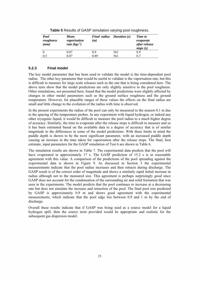
Table 5 Results of GASP simulation varying pool roughness. Pool roughness (mm)

Mean vaporisation rate (kgs-1)

Final radius (m)

Duration (s) Time to evaporate after release stops (s)

0 0.07 0.9 561 8.9 0.5 0.07 0.89 561 8.7

5.2.3 Final model The key model parameter that has been used to validate the model is the time-dependent pool radius. The other key parameter that would be useful to validate is the vaporisation rate, but this is difficult to measure for large scale releases such as the one that is being considered here. The above tests show that the model predictions are only slightly sensitive to the pool roughness. Other simulations, not presented here, found that the model predictions were slightly affected by changes in other model parameters such as the ground surface roughness and the ground temperature. However, for plausible ranges of these values the effects on the final radius are small and little change to the evolution of the radius with time is observed.

In the present experiments the radius of the pool can only be measured to the nearest 0.1 m due to the spacing of the temperature probes. In any experiment with liquid hydrogen, or indeed any other cryogenic liquid, it would be difficult to measure the pool radius to a much higher degree of accuracy. Similarly, the time to evaporate after the release stops is difficult to measure and so it has been estimated based on the available data to a degree of accuracy that is of similar magnitude to the differences in some of the model predictions. With these limits in mind the puddle depth is shown to be the most significant parameter, with an increased puddle depth causing an increase in the time taken for vaporisation after the release stops. The final, best estimate, input parameters for the GASP simulation of Test 6 are shown in Table 6.

The simulation results are shown in Table 7. The experimental data predicts that the pool will have evaporated in approximately 17 s. The GASP prediction of 15.2 s is in reasonable agreement with this value. A comparison of the predictions of the pool spreading against the experimental data is shown in Figure 9. As discussed in Section 3 the experimental measurements indicate that the pool radius increases and then retracts during discharge. The GASP result is of the correct order of magnitude and shows a similarly rapid initial increase in radius although not to the measured size. This agreement is perhaps surprisingly good since GASP does not account for the condensation of the surrounding air and solid formation that was seen in the experiments. The model predicts that the pool continues to increase at a decreasing rate but does not simulate the increase and retraction of the pool. The final pool size predicted by GASP is approximately 0.9 m and shows good agreement with the experimental measurements, which indicate that the pool edge lies between 0.9 and 1 m by the end of discharge.

Overall these results indicate that if GASP was being used as a source model for a liquid hydrogen spill, then the source term provided would be appropriate and realistic for the subsequent gas dispersion model.

24

Table 6 Final input into GASP for Test 6. Substrate Concrete Heat transfer Perfect thermal contact Puddle depth (mm) 5.0 Release type Continuous Pool roughness (m) 0.5 Substance Hydrogen Mass flow rate (kgs-1) 0.0707 Aperture diameter (m) 0.025 Duration (s) 561 Initial pool temperature (K) 20.4 Ambient temperature (K) 266 Wind speed (ms-1) 3 Surface roughness (mm) 0.5

Table 7 Results of GASP simulation using final input for Test 6. Mean vaporisation rate (kgs-1)

Final radius (m)

Release duration (s)

Time to evaporate after release stops (s)

0.07 0.89 561 15.2

Figure 9 Radius of the pool extracted from experimental measurements and as

predicted by GASP.

0

0.2

0.4

0.6

0.8

1

1.2

1.4

0 100 200 300 400 500 600

Time (s)

Poo

l rad

ius

(m)

Release stop

Radius (m)

GASP

25

Figure 10 Depth of the pool as predicted by GASP.

The pool depth predicted by GASP for the conditions in Table 6 is shown in Figure 10. After 561 s the pool depth is approximately constant at 0.006 m, or 0.001 m not standing in the puddles. It is not possible to approximate the depth of the pool from the experimental data. There are no interim probes between those at ground level and those used to measure the cloud concentration (1.5 m away and 0.25 m above ground level). Moreover, such a depth is likely to be of a similar magnitude to the accuracy of the instrumentation.

0

0.001

0.002

0.003

0.004

0.005

0.006

0.007

0.008

0.009

0.01

0 100 200 300 400 500 600

Time (s)

Dep

th (m

)Pool depth

Puddle depth

Release stop

26

6 CONCLUSIONS

The ability of the model GASP to simulate the liquid pool formed during a release of liquid hydrogen has been assessed. Firstly, the pool spreading was studied by extracting data from the experimental measurements undertaken at HSL and a simple analysis was performed using this information. Validation was first carried out of GASP predictions for heat flux and vaporisation of liquid hydrogen and oxygen using existing experimental data for a non-spreading pool. GASP was then used to predict the pool spreading and vaporisation of the liquid hydrogen release in Test 6 of the HSL experiments.

The simple analysis of the HSL experimental data shows that in the first 200 s a gravity current is formed of cold air which spreads ahead of the pool. Both the analysis and measurements suggest that this current will not be deeper than 0.5 m within 1.5 m from the release, assuming an approximately circular pool.

The preliminary validation test of vaporisation of a non-spreading pool showed good agreement for the heat flux between GASP and the experimental measurements of Takeno et al. (1994) for liquid hydrogen on a concrete substrate. The heat flux was found to change with time proportional to t-1/2. This study has noted that care must be taken when modelling zero wind scenarios since GASP was not designed to model these conditions. A wind speed of at least 0.1 ms-1 was required to achieve a valid result.

The thermal properties of the concrete used by Takeno et al. (1994) are not stated in their paper, and there is no record of how they measured them (or indeed whether they optimised them to fit the data). However, Takeno et al. (1994) do show (as GASP confirms) that the same values for the substrate cannot fit both the hydrogen and oxygen experiments. GASP’s default values for concrete fit the hydrogen results better than the oxygen and the oxygen appears to boil too quickly. However, given that different kinds of concrete can have different thermal properties, it may be more appropriate to choose the concrete properties to fit the oxygen results, and consider the possibility of imperfect thermal contact with the ground in the case of the liquid hydrogen.

In Test 6 liquid hydrogen was released through a nozzle orientated vertically towards the ground with release conditions of 60 lmin-1 for about 9 minutes. The experimental measurements show that the radius of the resulting pool expands rapidly to approximately 1 m. It then stays constant at this size for about 200 s before expanding to approximately 1.3 m and retracting back to 1 m over about 100 s. For the remainder of the release it remains at approximately 1 m. The GASP model predicts an initially increasing radius but more slowly than the measurements. The expansion and retraction of the pool that occurred during the release are likely to be due to the condensation of air and solid formation on the ground that were observed during the experiments. This behaviour is not accounted for in the GASP model but the agreement seen here suggests that ignoring this behaviour may be a reasonable assumption. However, the final pool radius predicted by GASP is of a similar order to that observed in the experiments and therefore would in theory provide a reasonable input to a subsequent model of the dispersion of the resulting gas/vapour.

After the release stops the measurements indicate that it takes approximately 17 s for the liquid to evaporate. The final evaporation occurs approximately simultaneously over the whole pool, although if a higher pool temperature is assumed there is evidence that it may retract from the centre outwards. GASP predicts that the pool will have evaporated in 15.2 s, which is in reasonable agreement with the measured value. However, the puddle depth selected in GASP

27

significantly affected this time. In fact, of the parameters varied, this had the most significant effect on the results.

Overall, the GASP model has provided reasonable predictions of a vertically downward release of liquid hydrogen. With further validation it could be a useful tool for providing source conditions for a subsequent dispersion analysis.

28

7 RECOMMENDATIONS

The conclusions drawn here are mainly based on the comparison of GASP with one experiment of a spreading vaporising hydrogen pool. For increased confidence in the model further validation needs to be undertaken both with liquid hydrogen and other cryogenic liquids. Additional measurements of the depth of the pool and the radius would be useful to increase confidence in the model.

The model GASP assumes a certain degree of user knowledge and does not place restrictions on user input. With this in mind, careful consideration should be given to the parameters selected and sensitivity tests are advised. In particular, the sensitivity of the results to the puddle depth should be assessed. Potential alternative approaches for estimating an appropriate puddle depth have been investigated recently in the context of spreading pools and it is recommended that this work is continued.

Further development of GASP to make it easier to model boiling pools in zero wind conditions would be useful.

Despite the reasonable agreement presented here, integral models such as GASP have limitations due to assumptions made in their derivation. In particular, as the model is axi-symmetric it is not suitable for scenarios with complex terrain. Other approaches such as 2D shallow layer models would add significant benefits in this respect without the complications associated with a fully 3D CFD model. Also, a model that was not exclusively axi-symmetric would mean that further measurement data from Royle and Willougby (2012), and other sources, could be used for more extensive validation.

29

8 REFERENCES

Arntzen, B.J. and Middha, P. 2008. Modelling of liquid H2 release and dispersion. GexCon Report 2008-F46207-TN-6.

Brambilla, S. and Manca, D. 2009. Accidents involving liquids: A step ahead in modelling pool spreading, evaporating and burning. Journal of Hazardous Materials. 161(2-3). 1265-1280.

Brighton, P.W.M. 1985. Evaporation from a plane liquid surface into a turbulent boundary layer. Journal of Fluid Mechanics. 159. 323-345.

Chirivella J.E., Witcofski R.D. 1986. Experimental Results from Fast 1500 Gallon LH2 spills. American Institute for Chemical Engineers Symposium 82(251). 120-140.

Chitose, K., Takeno, K., Yamada, Y., Hayashi, K. and Hishida, M. 2002a. Activities on hydrogen safety for the WE-NET project – Experiment and simulation of the hydrogen dispersion. Proceedings of the 14th World Hydrogen Energy Conference, Toronto, Canada.

Chitose, K., Okamoto, M., Takeno, K., Hayashi, K. and Hishida, M. 2002b. Analysis of a large scale liquid hydrogen dispersion using the multi-phase hydrodynamics analysis code (CHAMPAGNE). Journal of Energy Resources Technology. 124. 283 – 289.

Chitose, K., Ogawa, Y.and Morii, T. 1996. Analysis of a large scale liquid hydrogen spill experiment using the multi-phase hydrodynamics analysis code. Proceedings of the 11th World Hydrogen Energy Conference, Stuttgart, Germany.

FLACS. 2010. FLACS v9.1 User’s Manual. GexCon AS.

Gant, S.E. and Hoyes, J.R. 2009. Review of FLACS version 9.0: Dispersion modelling capabilities. HSL Report MSU/2009/06. Available from HSL: Buxton.

Gavelli, F., Chernovsky, M.K., Bullister, E., Kytomaa, H. K. 2009. Quantification of source-level turbulence during LNG spills onto a water pond. Journal of Loss Prevention in the Process Industries 22. 809-819.

Giannissi, S.G., Venetsanos, A.G., Bartzis, J.G., Markatos, N., Willoughby, D. and Royle, M. 2011. CFD modelling of LH2 dispersion using the ADREA-HF code. 4th International Conference on Hydrogen Safety, 12 – 14th September, San Fransisco, California.

Hall, J., Willoughby, D and Hooker, P. 2013. Ignited releases of liquid hydrogen. HSL Report XS/11/77. Available from HSL: Buxton.

Hanna, S.R. and Britter, R.E. 2002. Wind Flow and Vapour Cloud Dispersion at Industrial and Urban Sites. AIChE Centre for Chemical Process Safety. p 208.

Hansen, O.R., Melheim, J.A. and Storvik, I.E. 2007. CFD-Modelling of LNG dispersion experiments. AIChE Spring Meeting, 7th Topical Conference on Natural Gas Utilisation, Houston, Texas, 22 – 26 April.

Hijikata, T. 2002. Research and development of international clean energy network using hydrogen energy (WE-NET). International Journal of Hydrogen Energy. 27. 115 – 129.

30

Hissong, D. W. 2007. Keys to modelling LNG spills on water. Journal of Hazardous Materials. 140. 465-477

HSE. 2006. HSE Planning Case Assessment Guide, Chapter 5B: Modelling pool spreading and evaporation, Version 21, issued 11/04/2006

Ichard, M., Hansen, O.R., Middha, P. and Willoughby, D. 2011. CFD computations of liquid hydrogen releases. 4th International Conference on Hydrogen Safety, 12 – 14th September, San Fransisco, California.

Jäkel, C. 2011. Personal communication.

Marinescu – Pasoi, L. and Sturm, B. 1994. Messung der Ausbreitung earner Wassertoff-und Propanwolke in bebautem Gelaende. Battelle Ingenieurtechnik report R-68202

Marinescu – Pasoi, L. and Sturm, B. 1994. Gasspezifische Ausbreitungsversuche. Battelle Ingenieurtechnik Report R-68264

Middha, P., Ichard, M. and Arntzen, B.J. 2010. Validation of CFD modelling of LH2 spread and evaporation against large-scale spill experiments. Journal of Hydrogen Energy. P 1-8 (Article in press).

Molkov, V.V., Makarov, D.V. and Prost, E. 2005. On numerical simulation of liquefied and gaseous hydrogen releases at larger scales. International Conference of Hydrogen Safety, Pisa, Italy, Sept 8-10.

Moorhouse, J. and Carpenter, R.C. 1986. Factors affecting vapour evolution rates from liquefied gas spills. Proceedings of the IChemE (NW Branch) Conference on Refinement of Estimates of the Consequences of Heavy Toxic Vapour Releases.

Morii, T. and Ogawa, Y. 1996. Development and application of a fully implicit fluid dynamics code for multiphase flow. Nuclear Technology. 115. 333-341.

Schmidt, D., Krause, U. and Schmidtchen, U. 1999. Numerical simulation of hydrogen gas releases between buildings. International Journal of Hydrogen Energy. 24. 479-488.

Royle, M. and Willoughby, D. 2012. Releases of unignited liquid hydrogen. HSL Report XS/11/70. Available from HSL: Buxton.

Sklavounos, S. and Rigas, F. 2005. Fuel gas dispersion under cryogenic release conditions. Energy and Fuels. 19. 2535-2544.

Statharas J.C., Venetsanos A.G., Bartzis J.G., Würtz J., Schmidtchen U. 2000. Analysis of data from spilling experiments performed with liquid hydrogen. Journal of Hazardous Materials. A77(1–3). 57–75.

Takeno, K., Ichinose, T., Hyodo, Y. and Nakamura, H. 1994. Evaporation rates of liquid hydrogen and liquid oxygen spilled onto the ground. Journal of Loss Prevention in the Process Industries. 7(5). 425-431.

Venetsanos A.G., Bartzis J.G. 2007. CFD modelling of large-scale LH2 spills in open environment. International Journal of Hydrogen Energy. 32. 2171–7.

31

Venetsanos, A.G., Papanikolaou, E. and Bartzis, J.G. 2010. The ADREA-HF CFD code for consequence assessment of hydrogen applications. International Journal of Hydrogen Energy. 35(8). 3908-3918.

Verfondern, K. and Dienhart, B. 2007. Pool spreading and vaporisation of liquid hydrogen. International Journal of Hydrogen Energy. 32. 256-267.

Verfondern, K. and Dienhart, B. 1997. Experimental and theoretical investigation of liquid hydrogen pool spreading and vaporisation. International Journal of Hydrogen Energy. 22(7). 649-660.

Webber, D.M. 1990. A model for pool spreading and vaporisation and its implementation in the computer code GASP. SRD / HSE / R521.

Webber, D.M. and Jones, S.J. 1989. A users guide to GASP on microcomputers. SRD / HSE / R507.

Webber, D.M., Gant S.E., Ivings M.J. and Jagger, S. 2010. LNG source term models for hazard analysis: a review of the state of the art and an approach to model assessment. HSE Research Report RR789.

Webber, D.M., Jones, S.J., Tickle, G. A., Wren, T. 1992a. A model of a dispersing gas cloud, and the computer implementation DRIFT – I Near instantaneous releases. UKAEA Report SRD/HSE R586.

Webber, D.M., Jones, S.J., Tickle, G. A., Wren, T. 1992b. A model of a dispersing gas cloud, and the computer implementation DRIFT – II Steady continuous releases. UKAEA Report SRD/HSE R587.

Witcofski, R.D., Chirivella, J.E. 1984. Experimental and analytical analyses of the mechanisms governing the dispersion of flammable clouds formed by liquid hydrogen spills. International Journal of Hydrogen Energy 1984. 9(5). 425–35.

Published by the Health and Safety Executive 02/14

Modelling of liquid hydrogen spills

Health and Safety Executive

RR985

www.hse.gov.uk

In the long term the key to the development of a hydrogen economy is a full infrastructure to support it, which includes means for the delivery and storage of hydrogen at the point of use, eg at hydrogen refuelling stations for vehicles. As an interim measure to allow the development of refuelling stations and rapid implementation of hydrogen distribution to them, liquid hydrogen is considered the most efficient and cost effective means for transport and storage.

The Health and Safety Executive (HSE) have commissioned the Health and Safety Laboratory (HSL) to identify and address issues relating to bulk liquid hydrogen transport and storage and update/develop guidance for such facilities. The second phase of the project involved experiments on unignited (HSE RR986) and ignited releases of liquid hydrogen (HSE RR987) and computational modelling of the unignited releases. This position paper assesses the ability of the cryogenic liquid spill models available to the HSE to model spills of liquid hydrogen by using the new experimental data obtained from the experimental testing at HSL.

A brief literature review on modelling liquid hydrogen pool spread was undertaken and modelling with GASP (Gas Accumulation over Spreading Pools) to compare results with the experimental measurement data. Recommendations are made on improvements to currently available models and also recommendations for further model validation data.

This report and the work it describes were funded by the Health and Safety Executive. Its contents, including any opinions and/or conclusions expressed, are those of the authors alone and do not necessarily reflect HSE policy.