small-signal analysis of power systems with low … · p l power systems laboratory johanna vorwerk...
TRANSCRIPT

P LPowerSystemsLaboratory
Johanna Vorwerk
Small-Signal Analysis of Power Systems withLow Rotational Inertia
Semester ThesisPSL 1714
EEH – Power Systems LaboratorySwiss Federal Institute of Technology (ETH) Zurich
Expert: Prof. Dr. Gabriela HugSupervisors: M.Sc. Uros Markovic
Zurich, May 9, 2018
Abstract
Due to the increasing share of renewable energy generation units, the physical inertiais decreasing in not only distribution but also transmission grids, leading towards low-inertia systems. However, the existing control schemes for Voltage Source Converters(VSCs), the power electronic grid interface used for renewable generation, mostly focuson microgrids that have different requirements than transmission grids. In this contexta model for transmission grids is proposed.
We first present the VSC model used in this work and analytically describe eachcontrol block. The proposed model includes options to operate grid-forming and grid-feeding controllers and incorporates two different active power control schemes: activepower droop control and virtual inertia emulation. After linearizing the model in orderto apply standard control analysis, its implementation in MATLAB and verification isdiscussed. Having established the foundation, small-signal stability analyses are per-formed, showing that the converter configuration significantly affects stability margins.Besides optimizing the outer control loop parameters, the effect of the grid equivalenton overall system stability and the impact of the synchronization unit for grid-followingconverters are investigated. Simulations show that in general grid-forming convertersprovide larger stability margins. Indeed, grid-feeding converters operating with activepower droop may not retain stability when connected to weaker grids.
i

Contents
List of Acronyms iv
1 Introduction 1
2 Mathematical Model of the VSC 32.1 Control System Overview . . . . . . . . . . . . . . . . . . . . . . . . . . . 32.2 Modelling Conventions . . . . . . . . . . . . . . . . . . . . . . . . . . . . . 42.3 System Modelling . . . . . . . . . . . . . . . . . . . . . . . . . . . . . . . . 4
2.3.1 Electric System . . . . . . . . . . . . . . . . . . . . . . . . . . . . . 42.3.2 Power Calculation Unit . . . . . . . . . . . . . . . . . . . . . . . . 52.3.3 Active Power Control . . . . . . . . . . . . . . . . . . . . . . . . . 62.3.4 Reactive Power Control . . . . . . . . . . . . . . . . . . . . . . . . 72.3.5 Virtual Impedance . . . . . . . . . . . . . . . . . . . . . . . . . . . 82.3.6 Inner Control Loop and Modulation . . . . . . . . . . . . . . . . . 82.3.7 Phase Locked Loop . . . . . . . . . . . . . . . . . . . . . . . . . . . 92.3.8 Aligning Reference Frames . . . . . . . . . . . . . . . . . . . . . . 10
2.4 Operation Modes . . . . . . . . . . . . . . . . . . . . . . . . . . . . . . . . 112.5 Non-Linear System Model . . . . . . . . . . . . . . . . . . . . . . . . . . . 122.6 Linear Small-Signal Model . . . . . . . . . . . . . . . . . . . . . . . . . . . 13
3 Model Implementation and Verification 163.1 Model Implementation in MATLAB . . . . . . . . . . . . . . . . . . . . . 163.2 Model Parameters . . . . . . . . . . . . . . . . . . . . . . . . . . . . . . . 173.3 Model Verification . . . . . . . . . . . . . . . . . . . . . . . . . . . . . . . 17
3.3.1 Test Case I: Active Power Droop Control in Grid-Forming Operation 183.3.2 Test Case II: Virtual Inertia Emulation in Grid-Feeding Operation 19
4 Stability Analysis 204.1 Eigenvalues at Operation Point . . . . . . . . . . . . . . . . . . . . . . . . 204.2 Tuning the Power Control Loops . . . . . . . . . . . . . . . . . . . . . . . 22
4.2.1 Active Power Droop . . . . . . . . . . . . . . . . . . . . . . . . . . 224.2.2 Virtual Inertia Emulation . . . . . . . . . . . . . . . . . . . . . . . 23
4.3 Tuning PLL Control Parameters . . . . . . . . . . . . . . . . . . . . . . . 25
ii

CONTENTS iii
4.4 Influence of the Grid Equivalent . . . . . . . . . . . . . . . . . . . . . . . 264.4.1 Influence of the Grid Equivalent on APC Droop Control in g-feed
Operation . . . . . . . . . . . . . . . . . . . . . . . . . . . . . . . . 274.4.2 Influence of SCR on VIE Control in g-feed Operation . . . . . . . 28
5 Outlook and Conclusion 31
Bibliography 32

List of Acronyms
AC Alternating Current
APC Active Power Control
DAE Differential Algebraic Equation
DC Direct Current
g-feed Grid-Feeding Converter
g-form Grid-Forming Converter
LHP Left Half-Plane
LPF Low-Pass Filter
PLL Phase-Locked Loop
RPC Reactive Power Controller
SM Synchronous Machine
SCR Short Circuit Ratio
SRF Synchronous Reference Frame
SSM Small-Signal Model
VIE Virtual Inertia Emulation
VSC Voltage Source Converter
iv

List of Figures
2.1 Overview of investigated and implemented VSC-control structure. . . . . 42.2 APC control schemes: (a) APC droop control block and (b) VIE control
block. . . . . . . . . . . . . . . . . . . . . . . . . . . . . . . . . . . . . . . 62.3 Reactive power control block. . . . . . . . . . . . . . . . . . . . . . . . . . 72.4 PLL control block. . . . . . . . . . . . . . . . . . . . . . . . . . . . . . . . 102.5 Vector diagram defining the SRF and voltage vector orientation. . . . . . 11
3.1 Comparing the Simulink, DAE and SSM simulation results in the case ofAPC droop implementation for g-form converters. . . . . . . . . . . . . . 18
3.2 Comparing the Simulink, DAE and SSM simulation results in the case ofVIE implementation for g-feed converters. . . . . . . . . . . . . . . . . . . 19
4.1 Location of eigenvalues on imaginary plane for the given point of operationand different control options. . . . . . . . . . . . . . . . . . . . . . . . . . 21
4.2 Stability map of different converter modes on the Dp-Dq plane. Thesystem is stable in the shaded region. . . . . . . . . . . . . . . . . . . . . . 22
4.3 Critical eigenvalue λ for (a) g-form and (b) g-feed VSC operation of APCdroop control. . . . . . . . . . . . . . . . . . . . . . . . . . . . . . . . . . . 23
4.4 Movement of the critical eigenvalue λ with changing inertia for differentoperation modes and Kd = 1 p.u. . . . . . . . . . . . . . . . . . . . . . . . 24
4.5 Stability map of different converter modes in the H-Kd plane. The systemis stable in the shaded region. . . . . . . . . . . . . . . . . . . . . . . . . . 24
4.6 Stability surfaces for VIE control in different converter operation: inertiarequirement depending on damping constants and reactive power droopgains in (a) combined plot, (b) for grid-forming and (c) grid-feeding con-verter mode. . . . . . . . . . . . . . . . . . . . . . . . . . . . . . . . . . . 25
4.7 Critical inertia for varying PLL control parameters in g-feed VIE opera-tion for damping Kd = 10 p.u., equivalent to active droop Dp = 1%. . . . 26
4.8 SCR influence on critical eigenvalue with initial operation parameters fordifferent operation modes with model parameters specified in Tab. 3.1and xg/rg = 10. . . . . . . . . . . . . . . . . . . . . . . . . . . . . . . . . . 27
v

LIST OF FIGURES vi
4.9 Influence of active power droop gain and (a) SCR on critical eigenvalueand (b) resulting stability map on Dp-η plane: the shaded region is stable,with constant reactive droop Dq = 0.01%. . . . . . . . . . . . . . . . . . . 28
4.10 Influence of active and reactive power droop gains on critical SCR η∗: anyoperation point above the surface is stable. . . . . . . . . . . . . . . . . . 28
4.11 Influence of inertia emulation and SCR on critical eigenvalue; the param-eters for damping and inertia correspond to the active power gains inFig. 4.9a. . . . . . . . . . . . . . . . . . . . . . . . . . . . . . . . . . . . . 29
4.12 Critical SCR η∗ in dependence of inertiaH for different damping constantsKd. . . . . . . . . . . . . . . . . . . . . . . . . . . . . . . . . . . . . . . . . 29

List of Tables
2.1 Overview of operation modes and the changes imposed to the mathemat-ical model. . . . . . . . . . . . . . . . . . . . . . . . . . . . . . . . . . . . . 12
3.1 VSC model parameters. . . . . . . . . . . . . . . . . . . . . . . . . . . . . 17
4.1 Eigenvalues at operation point . . . . . . . . . . . . . . . . . . . . . . . . 21
vii
Chapter 1
Introduction
The increasing share of renewable generation units connected to the transmission gridsimultaneously extends the penetration of Voltage Source Converters (VSCs), that actas grid-interface. Due to their power electronic nature, the physical inertia of the gener-ators is progressively decoupled from the network, resulting in low inertia systems andimposing new challenges regarding system stability [1]. In order to capture the systemdynamics in the presence of these converters, new Differential-Algebraic Equation (DAE)models must be developed for the purpose of small-signal analysis.
The work in [2] investigated the stability of a VSC control scheme based on thevirtual swing equation. However, there was no external power control included in themodel, and the implementation of the damping restricted the applicability of the stud-ied control system. An extension of this control design was presented in [3], where afrequency droop was included in the outer loop, together with the Phase Locked Loop(PLL) and virtual impedance. The same control system and the corresponding small-signal model was further elaborated and analyzed in [4]. Nonetheless, both approachesfocus on a single power control design and put emphasis on the grid-connected opera-tion only. Since the potential VSC control configurations [5–7], as well as the operationmodes [8, 9] can be quite versatile, requirements for a more general modeling approachare emerging.
The contribution of this work is two-fold. First, we introduce a uniform VSC modelwith a detailed, state-of-the-art control structure. Two active power control approachesare proposed under different converter operation modes. Subsequently, a formulation ofthe DAE system, together with the respective small-signal model is derived. Second,the stability margins of different VSC configurations are investigated through eigenvalueanalysis and various bifurcation studies.
The remainder of the report is structured as follows. In Chapter 2, a detailed VSCcontrol scheme is presented, as well as the respective mathematical formulation of theproblem and the resulting DAEs. Furthermore, it describes the small-signal modelling
1

CHAPTER 1. INTRODUCTION 2
and derives the state-space representation. Chapter 3 outlines the implementation of thenon-linear and small-signal models in MATLAB, respectively. Moreover, it includes theoperation parameters and presents simulation results for the validation of the presentedmodels. Chapter 4 showcases the stability analyses results, whereas chapter 5 concludesthe thesis.

Chapter 2
Mathematical Model of the VSC
The objective of this chapter is to present the underlying VSC model that is usedthroughout this work. After giving a brief overall introduction of the control structure,the rest of the chapter focuses on each control block in detail by deriving its mathemat-ical model. In particular, power, voltage and current control, grid synchronization andpulse with modulation will be discussed. Besides examining the control elements, fourdistinct operation modes of the VSC will be introduced. Once the non-linear systemmodel is established, it will be linearized in order to perform a small-signal analysis inthe next chapter.
2.1 Control System Overview
An overview of the implemented converter control scheme is presented in Fig. 2.1, wherea VSC is connected to a constant active power load or a grid through a Low-Pass Filter(LPF) and a transformer. The outer control loop consists of active and reactive powercontrollers, which provide the output voltage angle and magnitude reference by adjust-ing the predefined setpoints according to a measured power imbalance. The referencevoltage signal is sent to the inner control loop, consisting of cascaded voltage and currentcontrollers, that operate in a Synchronously-rotating Reference Frame (SRF). In orderto detect the system frequency at the Point of Common Coupling (PCC), for synchro-nization a Phase-Locked Loop (PLL) unit is included in the model. For the purposesof mathematical description, an ideal average model of the Pulse Width Modulation(PWM) unit is assumed and switching is neglected. Moreover, the DC-side is assumednot to constrain the system and thus the energy source and storage on the DC-side areconsidered to be sufficient.
3

CHAPTER 2. MATHEMATICAL MODEL OF THE VSC 4
Cdc vdc
vg
Grid
dq
abc
dq
abc
idqg
PowerCalculation
Unitedqg
PhaseLockedLoop
SRFVoltage
Controller
SRFCurrent
ControllerPWM
ReactivePower
Controller
ActivePower
Controller
VirtualImpedance
Block
q∗
v∗
p∗
ω0
[edqg , i
dqg
]
θapc
Rt Lt
Rl
vm
idqs
Rf
Lf
Cf
iabcg
eabcg
is vm m
qp
ωapcvdc
v
v
ω∗ = [ω0, ωpll]
Inner control loopOuter control loop
Figure 2.1: Overview of investigated and implemented VSC-control structure.
2.2 Modelling Conventions
The complete description of the converter is based on per unit quantities, denoted bylower case letters. The upper case letters in Fig. 2.1 represent physical values of the elec-tric system. The entire modeling, analysis and control of the converter is implementedin an SRF, with the (abc/dq)-block designating a sequence of power-invariant Clarkeand Park transformations from a stationary (abc)-frame to the SRF. Quantities in theSRF are written in complex space vectors such as:
x = xd + jxq (2.1)
with the (dq) superscript omitted in the remainder of the report. However, stationaryreference frame quantities are always marked by the (abc) superscript. Additionally, theexternal control setpoints, e.g. the active power reference, are marked with x∗, whereasthe internally computed references are represented as x. The indicated current directionsin Fig. 2.1 result in positive active and reactive power quantities for an energy flow fromthe converter into the grid.
2.3 System Modelling
The following subsections present the non-linear mathematical model for each controlblock and system element in Fig. 2.1. Subsequently, the derived non-linear DAE-Modelwill be used to establish a linearized small-signal state-space model.
2.3.1 Electric System
The VSC can be operated in either island operation or grid connected mode, as indicatedin Fig. 2.1. In both cases, the electric system includes an LPF (rf , lf , cf ) and atransformer equivalent (rt, lt) to model copper and iron losses. The grid is modeled

CHAPTER 2. MATHEMATICAL MODEL OF THE VSC 5
as Thevenin equivalent, whereas the load is assumed to draw active power only. Thissimple structure is chosen to achieve a basic model focusing on the dynamics of theconverter rather than complex AC grid topology. The SRF state space equations for thegrid-connected case in pu-quantities and the SRF-coordinates can be established as:
is =ωblf
(vm − eg)−(rflfωb + jωbωg
)is (2.2)
ig =ωb
lg + lt(eg − vg)−
(rg + rtlg + lt
ωb + jωbωg
)ig (2.3)
eg =ωbcf
(is − ig)− jωgωbeg (2.4)
where is is the switching current flowing through the filter inductance, vm is the mod-ulation voltage at the converter output, ig is the current flowing into the grid, eg is thevoltage at the filter capacitors and vg is the voltage of the grid equivalent. The resistanceand inductance of the grid are denoted as rg and lg, while the grid and base frequencyare represented as ωg and ωb, respectively. For the sake of simplicity, the electric systemis modeled in the SRF defined by the Active Power Control (APC).
In case of island operation the electric system equations have to be modified. Ex-pression 2.3 changes to:
ig =ωblt
(eg − vg)−(rtltωb + jωbωg
)ig (2.5)
while defining the active load as a function of active power consumption pload and con-stant voltage amplitude v∗load as follows:
vg = rloadig =v∗load
2
ploadig (2.6)
It should be noted here that for a stand-alone operation the equivalent grid frequencyonly depends on the following factors: the external power and frequency setpoints, theactual load connected to the converter and the active power droop gain. Consequently,the overall system frequency is solely defined by the APC output.
2.3.2 Power Calculation Unit
The power calculation block processes measurements of grid voltage eg and grid currentig. Active and reactive power are calculated as follows:
p = <(egi′g) (2.7)
q = =(egi′g) (2.8)
where eg is the voltage at the filter capacitor and i′g is the complex conjugate of the gridcurrent.

CHAPTER 2. MATHEMATICAL MODEL OF THE VSC 6
2.3.3 Active Power Control
Since the focus of this work is on converter operation on a transmission grid level, theactive power control has been realized using two different approaches. On the one hand,the strong coupling of active power and frequency allows to use traditional droop control,which is the standard approach for frequency control in transmission grids nowadays.On the other hand, replicating the swing equation allows for virtual emulation of thebehaviour of a synchronous machine (SM), thereby recreating the inherit advantages ofSMs [10,11]. Virtual Inertia Emulation (VIE) is arising as one of the potential solutionsfor distribution and micro-grid applications.
p∗
p ωc
ωc+s
ω∗
Dp ωapc−−
p
(a)
p∗
p
ω∗
÷ 12H
Kd
1s
ωapc
ωb
s θapc
˙ωapc
−
−
−
(b)
Figure 2.2: APC control schemes: (a) APC droop control block and (b) VIE controlblock.
For active power droop control, described by the control structure in Fig. 2.2a, themeasured active power signal is passed through a first-order LPF with a cut-off frequencyωc. Subsequently, the active power droop gain Dp regulates the output frequency ωapcbased on the mismatch between the filtered power measurement signal p and the externalsetpoint p∗, as follows:
ωapc = ω∗ +Dp(p∗ − p) (2.9)
˙p = ωc(p− p) (2.10)
The second control scheme for virtual inertia emulation, illustrated in Fig. 2.2b,is based on a linearized conventional swing equation representing the relation betweenphysical inertia and damping of a traditional SM. For traditional SMs the accelerationof inertia H is determined by the balance of electrical pe, mechanical power pm anddamping power pd:
δω =1
2H(pm − pe − pd) (2.11)
where the mechanical and electrical power of the SM are replaced by the active powersetpoint p∗ and the active power output p fed into the grid. The damping term isincorporated through a feedback loop with a damping constant Kd. This feedbackgain is imposed on the frequency mismatch of the APC’s frequency output ωapc and
CHAPTER 2. MATHEMATICAL MODEL OF THE VSC 7
an external reference ω∗. The entire block diagram showing the implementation of theswing equation is presented in Fig. 2.2b. Ergo, the virtual acceleration of normalizedinertia can be formulated as:
δωapc =p∗
2H︸︷︷︸pm
− p
2H︸︷︷︸pe
− Kd
2H(ωapc − ω∗)
︸ ︷︷ ︸pd
(2.12)
In steady state there is neither frequency deviation nor active power mismatch. Thus,the frequency calculated by the APC ωapc is equal to grid frequency ωg and speeddeviation δωapc = ωapc − ωg vanishes. In case the converter is in island operation theAPC defines the grid frequency and speed deviation is set to zero. The correspondingphase angle θapc is defined by Eqn. 2.13 and used as a reference angle for the (dq)-transformation of the entire system, thereby avoiding switching between different SRFsand simplifying the model.
θapc = ωapcωb (2.13)
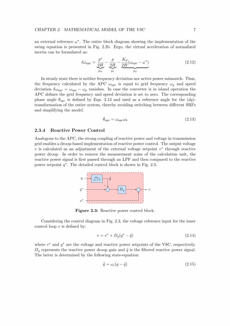
2.3.4 Reactive Power Control
Analogous to the APC, the strong coupling of reactive power and voltage in transmissiongrid enables a droop-based implementation of reactive power control. The output voltagev is calculated as an adjustment of the external voltage setpoint v∗ through reactivepower droop. In order to remove the measurement noise of the calculation unit, thereactive power signal is first passed through an LPF and then compared to the reactivepower setpoint q∗. The detailed control block is shown in Fig. 2.3.
q∗
q ωc
ωc+s
v∗
Dq v−
q
Figure 2.3: Reactive power control block.
Considering the control diagram in Fig. 2.3, the voltage reference input for the innercontrol loop v is defined by:
v = v∗ +Dq(q∗ − q) (2.14)
where v∗ and q∗ are the voltage and reactive power setpoints of the VSC, respectively.Dq represents the reactive power droop gain and q is the filtered reactive power signal.The latter is determined by the following state-equation:
˙q = ωc(q − q) (2.15)

CHAPTER 2. MATHEMATICAL MODEL OF THE VSC 8
where ωc represents the cut-off frequency of the LPF and q is the measured reactivepower.
2.3.5 Virtual Impedance
The virtual impedance concept is increasingly used for the control of power electronicsystems, either embedded as an additional degree of freedom for active stabilization anddisturbance rejection, or employed as a command reference generator for the convertersto provide ancillary services [12]. In this thesis, virtual impedance was included in orderto split the voltage amplitude reference v into (dq)-components, before passing it tothe SRF voltage control. Despite maximizing active power output when set to zero, anon-zero q-component is necessary to allow for “acceleration” and “deceleration” of thevirtual machine. Accordingly, minor cross-coupling of d- and q-components is needed.The virtual impedance includes a resistive rv and an inductive element lv. While theformer is set to zero to minimize active power loss, the latter should be kept as small asfeasible. The resulting d-axis and q-axis voltage components vd and vq
vd = v − rvidg + ωapclviqg (2.16)
vq = −rviqg + ωapclvidg (2.17)
are directly used as reference for the decoupling SRF voltage controller.
2.3.6 Inner Control Loop and Modulation
The computed references for voltage, frequency and transformation angle are passed tothe inner control loop as indicated in Fig 2.1. However, a direct use of such signals forPulse-Width Modulation raises problems regarding the limitations and controlled satura-tion of the converter’s currents and voltages [13]. These issues are conveniently resolvedwith a cascaded inner control scheme where the initial reference v is processed througha sequence of voltage and current loops, yielding a more robust converter setpoint vm.Such approach increases the flexibility of protection strategies and is commonly used indroop-controlled microgrids [7, 14].
SRF Voltage control
The structure of the SRF voltage controller follows the similar principles as the con-trollers in [3, 13]. The PI-controller acts on the mismatch of voltage reference v andmeasurement eg and includes the possibility to enable or disable a feed-forward of themeasured current feed-forward by setting the feed-forward gain Kffc ∈ [0, 1]. The refer-ence switching current is is given by:
is = Kpv(v − eg) +Kivξ + jcfωapceg +Kffcig (2.18)
ξ = v − eg (2.19)

CHAPTER 2. MATHEMATICAL MODEL OF THE VSC 9
where Kpv and Kiv are the proportional and the integral controller gains, respectively.The integrator state is represented by ξ.
SRF Current Control
Similar to its voltage counterpart, the following SRF current controller is a conventionalPI-controller with decoupling term. The modulation voltage reference vm is defined by:
vm = Kpc(is − is) +Kicγ + jlfωapcis +Kffveg (2.20)
γ = is − is (2.21)
where Kpc and Kic are the proportional and integral current gains, γ is the integratorstate and Kffv the voltage feed-forward. The generated output voltage reference vm isused to determine the final modulation signal.
Pulse-Width Modulation
For the purpose of an actual implementation of the VSC switching sequence, the voltagereference signal vm from the current controller must be processed and converted into themodulation index m. This can be achieved through means of instantaneous averagingapplied to the output voltage of the converter. Furthermore, the time delay effect ofPWM is neglected, which yields the following expression:
m =vmvDC
(2.22)
Neglecting any switching operation and assuming ideal PWM implementation withoutdelays, the averaged instantaneous converter modulation voltage vm is given by:
vm ≈m · vDC → vm ≈ vm (2.23)
Under these assumptions the reference modulation voltage will be close to the modulationvoltage itself, thereby completely decoupling the DC side from the converter model.Hence, it is not necessary to further model the DC side of the system. Nonetheless, inreal operation the DC side is required to provide sufficient energy storage and mightimpose restrictions [3].
2.3.7 Phase Locked Loop
The PLL or synchronizing unit is implemented as a Type-2 PLL, used to estimate thegrid frequency and keep the VSC synchronized to the grid [15]. The control structureis given in Fig. 2.4. The PLL uses a rather simple estimation scheme: It includes anindependent, internal (dq)-transformation that transforms the stationary output voltageeabcg . A PI-controller (Kp,pll, Ki,pll) is used to keep the q-component of the voltage zero.

CHAPTER 2. MATHEMATICAL MODEL OF THE VSC 10
The synchronization is achieved by aligning the d-axis of the internal SRF with the sta-tionary (abc)-frame and diminishing the q-component, as described in [9].
abc
dq
abc
dqeabcg
ω0
Kp,pll
Ki,pll
s
ωpll
ω0
ωb
s
edqgedg
eqg
θpll
Figure 2.4: PLL control block.
The estimated frequency ωpll is given by Eqn. 2.24, where ε is the integrator state.The transformation angle θpll is described by the state equation in Eqn. 2.26. It shouldbe noted here, that the (dq)-transformation of the PLL is completely independent of thetransformation used for the electrical circuit, hence adds a second SRF to the system.The alignment of these two SRFs further discussed in the next section.
ωpll = ω0 +Kp,plleqg,pll +Ki,pllε (2.24)
ε = eqg,pll (2.25)
θpll = ωpllωb (2.26)
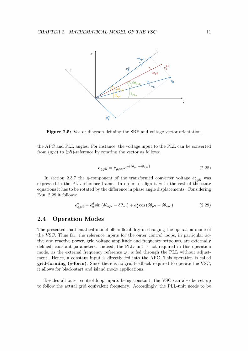
2.3.8 Aligning Reference Frames
The entire control system is implemented in the SRF defined by the APC output. Whenthe system is in steady state the APC calculated frequency ωapc equals the grid fre-quency, thus the corresponding angle θapc is chosen as a transformation angle to keepthe system as simple as possible. All states in the presented model rotate with thisfrequency except the ones included in the PLL unit, since it inherits its own transfor-mation. Consequently, the two transformations have to be properly aligned as shown inthe vector diagram in Fig. 2.5.
The systems reference frame and its phase angle displacement δθapc are defined withrespect to the voltage of a grid equivalent vg. Considering the reference amplitude ofthe grid voltage v∗g the vector in the APC-oriented reference frame can be expressed as:
vg = v∗ge−jδθapc (2.27)
The PLL reference frame and its phase angle displacement δθpll are defined withrespect to the same voltage vector. According to the definitions presented in Fig. 2.5 theangle difference between the two rotating reference frames is equal to the difference of
CHAPTER 2. MATHEMATICAL MODEL OF THE VSC 11
α
𝛽
𝑣g𝜔g
𝑒gpll
𝜔pll
𝛿𝜃PLL
𝜃PLL𝜃apc
𝛿𝜃apc
𝑑
𝑣g𝑞
𝑞 𝑣g𝑑
𝜔apc
Figure 2.5: Vector diagram defining the SRF and voltage vector orientation.
the APC and PLL angles. For instance, the voltage input to the PLL can be convertedfrom (apc) tp (pll)-reference by rotating the vector as follows:
eg,pll = eg,apce−(δθpll−δθapc) (2.28)
In section 2.3.7 the q-component of the transformed converter voltage eqg,pll wasexpressed in the PLL-reference frame. In order to align it with the rest of the stateequations it has to be rotated by the difference in phase angle displacements. ConsideringEqn. 2.28 it follows:
eqq,pll = edg sin (δθapc − δθpll) + egg cos (δθpll − δθapc) (2.29)
2.4 Operation Modes
The presented mathematical model offers flexibility in changing the operation mode ofthe VSC. Thus far, the reference inputs for the outer control loops, in particular ac-tive and reactive power, grid voltage amplitude and frequency setpoints, are externallydefined, constant parameters. Indeed, the PLL-unit is not required in this operationmode, as the external frequency reference ω0 is fed through the PLL without adjust-ment. Hence, a constant input is directly fed into the APC. This operation is calledgrid-forming (g-form). Since there is no grid feedback required to operate the VSC,it allows for black-start and island mode applications.
Besides all outer control loop inputs being constant, the VSC can also be set upto follow the actual grid equivalent frequency. Accordingly, the PLL-unit needs to be
CHAPTER 2. MATHEMATICAL MODEL OF THE VSC 12
activated, estimates the frequency and passes the result ωpll to the APC. This operationmode is called grid-feeding(g-feed) or grid-following operation, since a grid con-nection is required for stable operation. Consequently, the converter looses black-startpossibility. The VSC can only operate when connected to frequency reference, lackingthe option to supply a load in islanded operation.
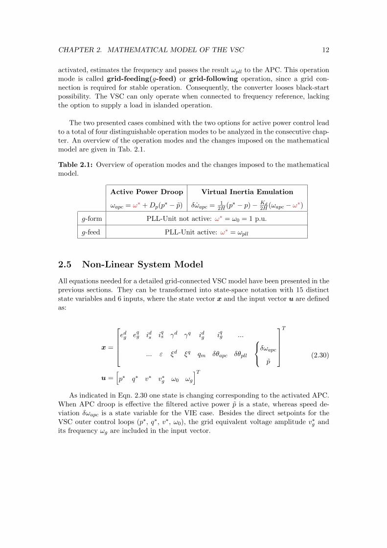
The two presented cases combined with the two options for active power control leadto a total of four distinguishable operation modes to be analyzed in the consecutive chap-ter. An overview of the operation modes and the changes imposed on the mathematicalmodel are given in Tab. 2.1.
Table 2.1: Overview of operation modes and the changes imposed to the mathematicalmodel.
Active Power Droop Virtual Inertia Emulation
ωapc = ω∗ +Dp(p∗ − p) δωapc = 1
2H (p∗ − p)− Kd2H (ωapc − ω∗)
g-form PLL-Unit not active: ω∗ = ω0 = 1 p.u.
g-feed PLL-Unit active: ω∗ = ωpll
2.5 Non-Linear System Model
All equations needed for a detailed grid-connected VSC model have been presented in theprevious sections. They can be transformed into state-space notation with 15 distinctstate variables and 6 inputs, where the state vector x and the input vector u are definedas:
x =
edg eqg ids iqs γd γq idg iqg ...
... ε ξd ξq qm δθapc δθpll
δωapc
p
T
u =[p∗ q∗ v∗ v∗g ω0 ωg
]T
(2.30)
As indicated in Eqn. 2.30 one state is changing corresponding to the activated APC.When APC droop is effective the filtered active power p is a state, whereas speed de-viation δωapc is a state variable for the VIE case. Besides the direct setpoints for theVSC outer control loops (p∗, q∗, v∗, ω0), the grid equivalent voltage amplitude v∗g andits frequency ωg are included in the input vector.
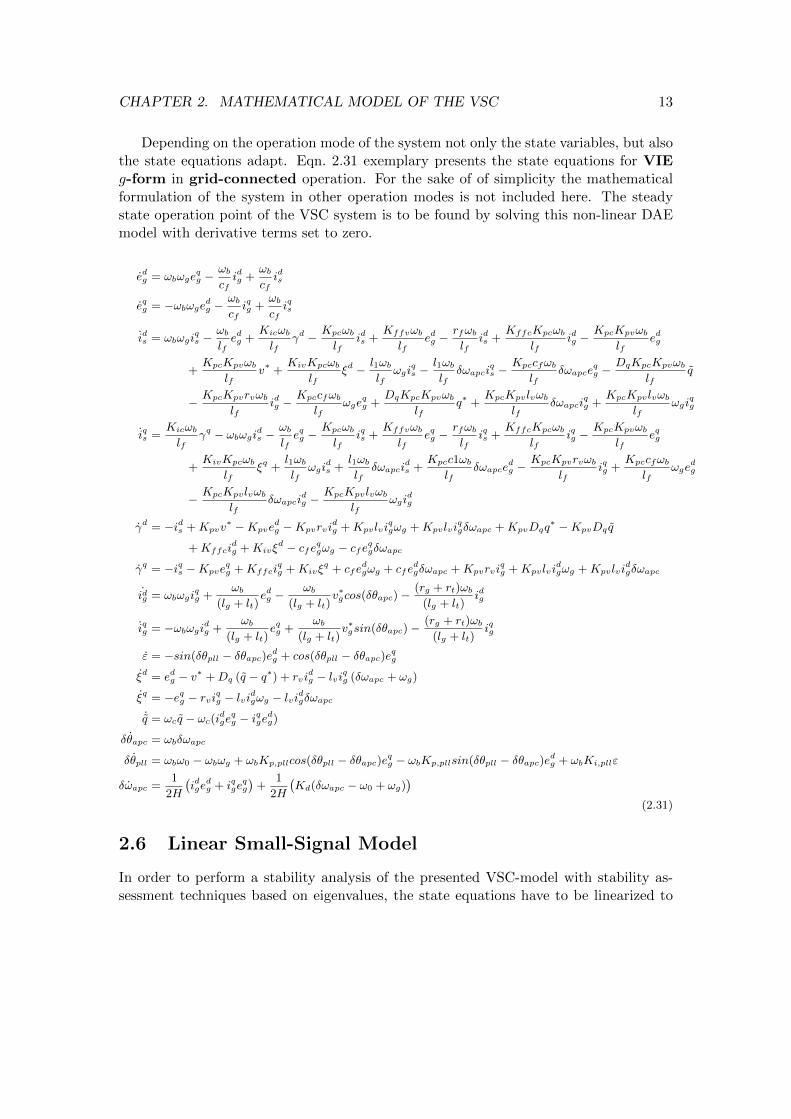
CHAPTER 2. MATHEMATICAL MODEL OF THE VSC 13
Depending on the operation mode of the system not only the state variables, but alsothe state equations adapt. Eqn. 2.31 exemplary presents the state equations for VIEg-form in grid-connected operation. For the sake of of simplicity the mathematicalformulation of the system in other operation modes is not included here. The steadystate operation point of the VSC system is to be found by solving this non-linear DAEmodel with derivative terms set to zero.
edg = ωbωgeqg − ωb
cfidg +
ωb
cfids
eqg = −ωbωgedg − ωb
cfiqg +
ωb
cfiqs
ids = ωbωgiqs −
ωb
lfedg +
Kicωb
lfγd − Kpcωb
lfids +
Kffvωb
lfedg − rfωb
lfids +
KffcKpcωb
lfidg − KpcKpvωb
lfedg
+KpcKpvωb
lfv∗ +
KivKpcωb
lfξd − l1ωb
lfωgi
qs −
l1ωb
lfδωapci
qs −
Kpccfωb
lfδωapce
qg − DqKpcKpvωb
lfq
− KpcKpvrvωb
lfidg − Kpccfωb
lfωge
qg +
DqKpcKpvωb
lfq∗ +
KpcKpvlvωb
lfδωapci
qg +
KpcKpvlvωb
lfωgi
qg
iqs =Kicωb
lfγq − ωbωgi
ds − ωb
lfeqg − Kpcωb
lfiqs +
Kffvωb
lfeqg − rfωb
lfiqs +
KffcKpcωb
lfiqg − KpcKpvωb
lfeqg
+KivKpcωb
lfξq +
l1ωb
lfωgi
ds +
l1ωb
lfδωapci
ds +
Kpcc1ωb
lfδωapce
dg − KpcKpvrvωb
lfiqg +
Kpccfωb
lfωge
dg
− KpcKpvlvωb
lfδωapci
dg − KpcKpvlvωb
lfωgi
dg
γd = −ids +Kpvv∗ −Kpve
dg −Kpvrvi
dg +Kpvlvi
qgωg +Kpvlvi
qgδωapc +KpvDqq
∗ −KpvDq q
+Kffcidg +Kivξ
d − cfeqgωg − cfe
qgδωapc
γq = −iqs −Kpveqg +Kffci
qg +Kivξ
q + cfedgωg + cfe
dgδωapc +Kpvrvi
qg +Kpvlvi
dgωg +Kpvlvi
dgδωapc
idg = ωbωgiqg +
ωb
(lg + lt)edg − ωb
(lg + lt)v∗gcos(δθapc) −
(rg + rt)ωb
(lg + lt)idg
iqg = −ωbωgidg +
ωb
(lg + lt)eqg +
ωb
(lg + lt)v∗gsin(δθapc) −
(rg + rt)ωb
(lg + lt)iqg
ε = −sin(δθpll − δθapc)edg + cos(δθpll − δθapc)e
qg
ξd = edg − v∗ +Dq (q − q∗) + rvidg − lvi
qg (δωapc + ωg)
ξq = −eqg − rviqg − lvi
dgωg − lvi
dgδωapc
˙q = ωcq − ωc(idge
qg − iqge
dg)
δθapc = ωbδωapc
δθpll = ωbω0 − ωbωg + ωbKp,pllcos(δθpll − δθapc)eqg − ωbKp,pllsin(δθpll − δθapc)e
dg + ωbKi,pllε
δωapc =1
2H
(idge
dg + iqge
qg
)+
1
2H
(Kd(δωapc − ω0 + ωg)
)(2.31)
2.6 Linear Small-Signal Model
In order to perform a stability analysis of the presented VSC-model with stability as-sessment techniques based on eigenvalues, the state equations have to be linearized to

CHAPTER 2. MATHEMATICAL MODEL OF THE VSC 14
obtain the small-signal state-space form:
∆x = A∆x+B∆u (2.32)
where a prefix ∆ denotes the small deviations of the system states around the steady-state operating point x0. The resulting algebraic state-space matrices for the case pre-sented in Eqn. 2.31 (VIE-control, g-form) are exemplary showcased at this point.Initial operation conditions of the states are denoted by subscript 0 in the matrix ele-ments. The matrices follow the scheme:
∆x1
∆x2
=
A11 A12
A21 A22
∆x1
∆x2
+B∆u (2.33)
A11 =
0 ωbωg0ωbcf
0 0 0 −ωbcf
−ωbωg0 0 0 ωbcf
0 0 0
ωb(Kffv−KpcKpv−1)lf
−Kpccfωbωlf
−ωb(rf+Kpc)lf
ωb (ωg0 − ω) Kicωblf
0Kpcωb(Kffi−Kpvrv)
lfKpccfωbω
lf
ωb(Kffv−KpcKpv−1)lf
ωb (ω − ωg0)ωb(−rf−Kpc)
lf0 −Kicωb
lf
−KpcKpvlvωbωlf
−Kpv −cf ω −1 0 0 0 Kffi −Kpvrv
cf ω −Kpv 0 −1 0 0 −Kpvlvω
ωblg+lt
0 0 0 0 0−ωb(rg+rt)
lg+lt
0 ωblg+lt
0 0 0 0 −ωbωg0
A12 =
0 0 0 0 0 0 0 0
−ωbcf
0 0 0 0 0 0 0
KpcKpvlvωbωlf
0 0KivKpcωb
lf0−DqKpcKpvωb
lf
−ωb(iqs0lf+Kpc(cf eqg0−Kpviqg0lv))
lf0
Kpvlvω 0 0 0KivKpcωb
lf0
ωb(ids0lf+Kpc(cf edg0−Kpvidg0lv))lf
0
Kffi −Kpcrv 0 0 Kiv 0 −DqKpv Kpviqg0lv − cfe0
g0 0
ωbωg0 0 0 0 Kiv 0 cfedg0 −Kpvi
qg0lv 0
−ωb(rg+rt)lg+lt
0v∗g0ωb sin (δθapc0)
lg+lt0 0 0 0 0
0 0v∗g0ωb cos (δθapc0)
lg+lt0 0 0 0 0
A21 =
− sin (∆θ0) cos (∆θ0) 0 0 0 0 0
0 0 0 0 0 0 0
−1 0 0 0 0 0 −rv0 −1 0 0 0 0 −lvω
−iqg0ωf idg0ωf 0 0 0 0 eqg0ωf
− idg02H − iqg0
2H 0 0 0 0 − edg02H
−Kp,pllωb sin (∆θ0) −Kp,pllωb cos (∆θ0) 0 0 0 0 0
A22 =
0 0 edg0 cos (∆θ0) + eqg0 sin (∆θ0) 0 0 0 0 −edg0 cos (∆θ0)− eqg0 sin (∆θ0)
0 0 0 0 0 0 ωb 0
lvω 0 0 0 0 −Dq iqg0lv 0
−rv 0 0 0 0 0 idg0lv 0
−edg0ωf 0 0 0 0 −ωf 0 0
− eqg02H 0 0 0 0 0 −Kd
2H 0
0 Ki,pllωb Kp,pllωb
(edg0 cos (∆θ0) + eqg0 sin (∆θ0)
)0 0 0 0 −Kp,pllωb
(edg0 cos (∆θ0) + eqg0 sin (∆θ0)
)

CHAPTER 2. MATHEMATICAL MODEL OF THE VSC 15
B =
0 0 0 0 0 eqg0ωb
0 0 0 0 0 −edg0ωb0
DqKpcKpvωb
lf
KpcKpvωb
lf0 0
−ωb(Kpc(cf eqg0−Kpvi
qg0lv))
lf
0 0 0 0 0ωbKpc(cf e
dg0−Kpvidg0lv)
lf
0 DqKpv Kpv 0 0 Kpviqg0lv − cfeqg0
0 0 0 0 0 cfedg0 −Kpvi
dg0lv
0 0 0 0 −ωb cos (δθapc0)lg+lt
iqg0ωb
0 0 0 0ωb sin (δθapc0)
lg+ltidg0ωb
0 0 0 0 0 0
0 0 0 0 0 0
0 Dq 1 0 0 iqg0lv
0 0 0 0 0 −idg0lv0 0 0 0 0 0
12H 0 0 Kd
2H 0 −Kd2H
0 0 0 ωb 0 −ωb
where the following substitutions were used:
∆θ0 = δθpll0 − δθapc0ω = δωapc0 + ωg0
Chapter 3
Model Implementation andVerification
This chapter focuses on the model implementation and verification. First, the implemen-tation of the non-linear DAE-model and the linearized small-signal model in MATLABis briefly explained. Then, after introducing the model parameters, the two models areverified for two test cases.
3.1 Model Implementation in MATLAB
For the scope of this thesis not only the presented DAEs in Eqn. 2.31, but also the stateequations for the remainder of operation modes were implemented in MATLAB, adapt-ing the procedure in [16, 17] and applying ODE-solver ode15s. This particular solver isneeded in order to solve a stiff system and allow for step inputs. After adjusting theinitial conditions close enough to the actual operating point, the ODE-solver deliversprecise results for both transient and steady-state operation. Simulation results are dis-cussed and presented in the model verification in chapter 3.3. Whenever results of thenon-linear mathematical model are presented in the proceeding sections, they will bemarked as DAE.
The linearized state-space model and its matrices are derived directly on run-time inMATLAB. Therefore, the procedure presented in [18] is adapted. The same state equa-tions as for the DAE-model are used to first calculate the symbolic systems’ Jacobianmatrix. In a second step all parameters and steady state operation point (x0,u0) arebeing replaced by their numerical values in order to calculate the numerical elementsof the state-space matrices. The operation point itself is determined by using the non-linear DAE-Model. Whenever results of the linearized small-signal model are shown inthe subsequent sections, they will be marked as SSM.
16
CHAPTER 3. MODEL IMPLEMENTATION AND VERIFICATION 17
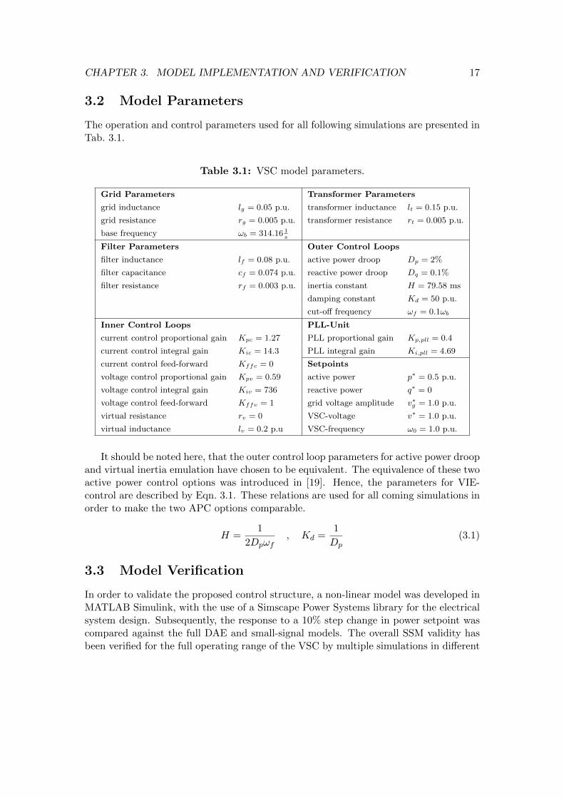
3.2 Model Parameters
The operation and control parameters used for all following simulations are presented inTab. 3.1.
Table 3.1: VSC model parameters.
Grid Parameters Transformer Parameters
grid inductance lg = 0.05 p.u. transformer inductance lt = 0.15 p.u.
grid resistance rg = 0.005 p.u. transformer resistance rt = 0.005 p.u.
base frequency ωb = 314.16 1s
Filter Parameters Outer Control Loops
filter inductance lf = 0.08 p.u. active power droop Dp = 2%
filter capacitance cf = 0.074 p.u. reactive power droop Dq = 0.1%
filter resistance rf = 0.003 p.u. inertia constant H = 79.58 ms
damping constant Kd = 50 p.u.
cut-off frequency ωf = 0.1ωb
Inner Control Loops PLL-Unit
current control proportional gain Kpc = 1.27 PLL proportional gain Kp,pll = 0.4
current control integral gain Kic = 14.3 PLL integral gain Ki,pll = 4.69
current control feed-forward Kffc = 0 Setpoints
voltage control proportional gain Kpv = 0.59 active power p∗ = 0.5 p.u.
voltage control integral gain Kiv = 736 reactive power q∗ = 0
voltage control feed-forward Kffv = 1 grid voltage amplitude v∗g = 1.0 p.u.
virtual resistance rv = 0 VSC-voltage v∗ = 1.0 p.u.
virtual inductance lv = 0.2 p.u VSC-frequency ω0 = 1.0 p.u.
It should be noted here, that the outer control loop parameters for active power droopand virtual inertia emulation have chosen to be equivalent. The equivalence of these twoactive power control options was introduced in [19]. Hence, the parameters for VIE-control are described by Eqn. 3.1. These relations are used for all coming simulations inorder to make the two APC options comparable.
H =1
2Dpωf, Kd =
1
Dp(3.1)
3.3 Model Verification
In order to validate the proposed control structure, a non-linear model was developed inMATLAB Simulink, with the use of a Simscape Power Systems library for the electricalsystem design. Subsequently, the response to a 10% step change in power setpoint wascompared against the full DAE and small-signal models. The overall SSM validity hasbeen verified for the full operating range of the VSC by multiple simulations in different

CHAPTER 3. MODEL IMPLEMENTATION AND VERIFICATION 18
operation modes. The consecutive subsections present the simulation results for twoselected operation modes.
3.3.1 Test Case I: Active Power Droop Control in Grid-Forming Op-eration
In this test case a step change in power setpoint of 0.1 p.u. at t = 1 s was simulatedwith the g-form APC converter model and the parameters given in Tab. 3.1. The plotsin Fig. 3.1 present the simulation results for grid voltage and current amplitudes, theirdq-composition and active, reactive power and frequency.
0 0.5 1 1.5 2
0.95
1
1.05
t [s]
Eg[p.u.]
Simulink
DAE
SSM
0 0.5 1 1.5 20
0.2
0.4
0.6
t [s]
I g[p.u.]
Simulink
DAE
SSM
0 0.5 1 1.5 20
0.2
0.4
0.6
t [s]
p[p.u.]
Simulink
DAE
SSM
0 0.5 1 1.5 2
0.95
1
1.05
t [s]
Ed g[p.u.]
Simulink
DAE
SSM
0 0.5 1 1.5 20
0.2
0.4
0.6
t [s]
Id g[p.u.]
Simulink
DAE
SSM
0 0.5 1 1.5 2
−0.1
0
0.1
t [s]
q[p.u.]
Simulink
DAE
SSM
0 0.5 1 1.5 2
−0.2
−0.1
0
t [s]
Eq g[p.u.]
Simulink
DAE
SSM
0 0.5 1 1.5 2−0.2
−0.1
0
0.1
t [s]
Iq g[p.u.]
Simulink
DAE
SSM
0 0.5 1 1.5 2
0.9
1
1.1
t [s]
f[p.u.]
Simulink
DAE
SSM
Figure 3.1: Comparing the Simulink, DAE and SSM simulation results in the case ofAPC droop implementation for g-form converters.
Obviously, the initialization of the Simulink and DAE-model take up to 0.3 s, eventhough most states initially obtain the correct steady state value. Nonetheless, the dy-namic behaviour during the initialization period of those two models is identical for allstates except frequency. The SSM does not show any initializing disturbances, as theoperation point is directly fed to the system by the DAE simulation output.
Of more importance for system validity is the reference step change in active powerat t = 1 s. Repeatedly, the transients occurring for all states except frequency are iden-tical. While no discrepancies exist when comparing the non-linear DAE-model to theSSM, minor differences are observable when comparing the SSM to the Simulink model.The latter is most visible for the q-component of the converter output voltage eqg. Con-sidering these scale of the plot, these differences are negligible.
CHAPTER 3. MODEL IMPLEMENTATION AND VERIFICATION 19
The inconsistency for frequency dynamics result from the use of Simulink controlblocks. These are sensitive to changes in frequency, hence result in larger overshoots.Since DAE and SSM still deliver consistent outcomes, the frequency mismatch of theSimulink model is considered not to contradict the SSM accuracy.
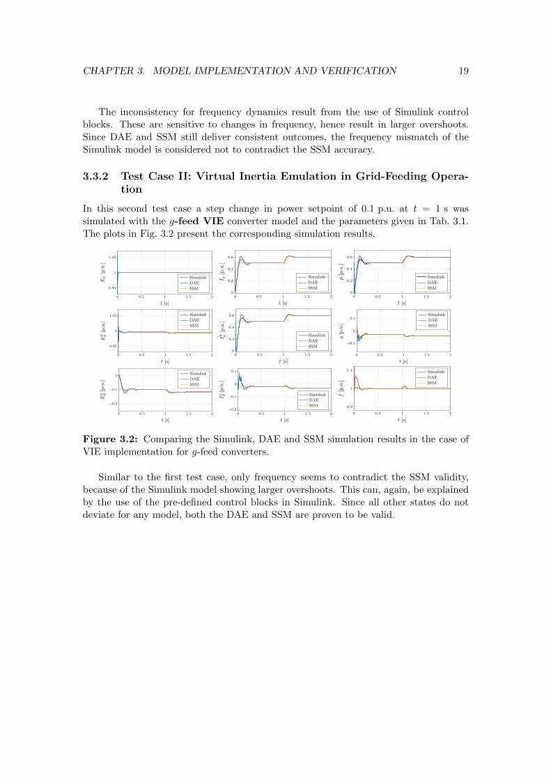
3.3.2 Test Case II: Virtual Inertia Emulation in Grid-Feeding Opera-tion
In this second test case a step change in power setpoint of 0.1 p.u. at t = 1 s wassimulated with the g-feed VIE converter model and the parameters given in Tab. 3.1.The plots in Fig. 3.2 present the corresponding simulation results.
0 0.5 1 1.5 2
0.95
1
1.05
t [s]
Eg[p.u.]
Simulink
DAE
SSM
0 0.5 1 1.5 20
0.2
0.4
0.6
t [s]
I g[p.u.]
Simulink
DAE
SSM
0 0.5 1 1.5 20
0.2
0.4
0.6
t [s]
p[p.u.]
Simulink
DAE
SSM
0 0.5 1 1.5 2
0.95
1
1.05
t [s]
Ed g[p.u.]
Simulink
DAE
SSM
0 0.5 1 1.5 20
0.2
0.4
0.6
t [s]
Id g[p.u.]
Simulink
DAE
SSM
0 0.5 1 1.5 2
−0.1
0
0.1
t [s]
q[p.u.]
Simulink
DAE
SSM
0 0.5 1 1.5 2
−0.2
−0.1
0
t [s]
Eq g[p.u.]
Simulink
DAE
SSM
0 0.5 1 1.5 2−0.2
−0.1
0
0.1
t [s]
Iq g[p.u.]
Simulink
DAE
SSM
0 0.5 1 1.5 2
0.9
1
1.1
t [s]
f[p.u.]
Simulink
DAE
SSM
Figure 3.2: Comparing the Simulink, DAE and SSM simulation results in the case ofVIE implementation for g-feed converters.
Similar to the first test case, only frequency seems to contradict the SSM validity,because of the Simulink model showing larger overshoots. This can, again, be explainedby the use of the pre-defined control blocks in Simulink. Since all other states do notdeviate for any model, both the DAE and SSM are proven to be valid.
Chapter 4
Stability Analysis
In this Chapter, the feasibility of the proposed linearized VSC converter model for thedifferent operation modes is investigated. After analyzing the eigenvalues at the initialoperating point, both APC control schemes are further studied by performing severalparameter sweeps. Furthermore, the RPC parameters are tuned and the impact of PLLparameters is examined. Finally, the effect of the grid equivalent on overall converterstability in combination with the different APC control and frequency control schemesis analyzed.
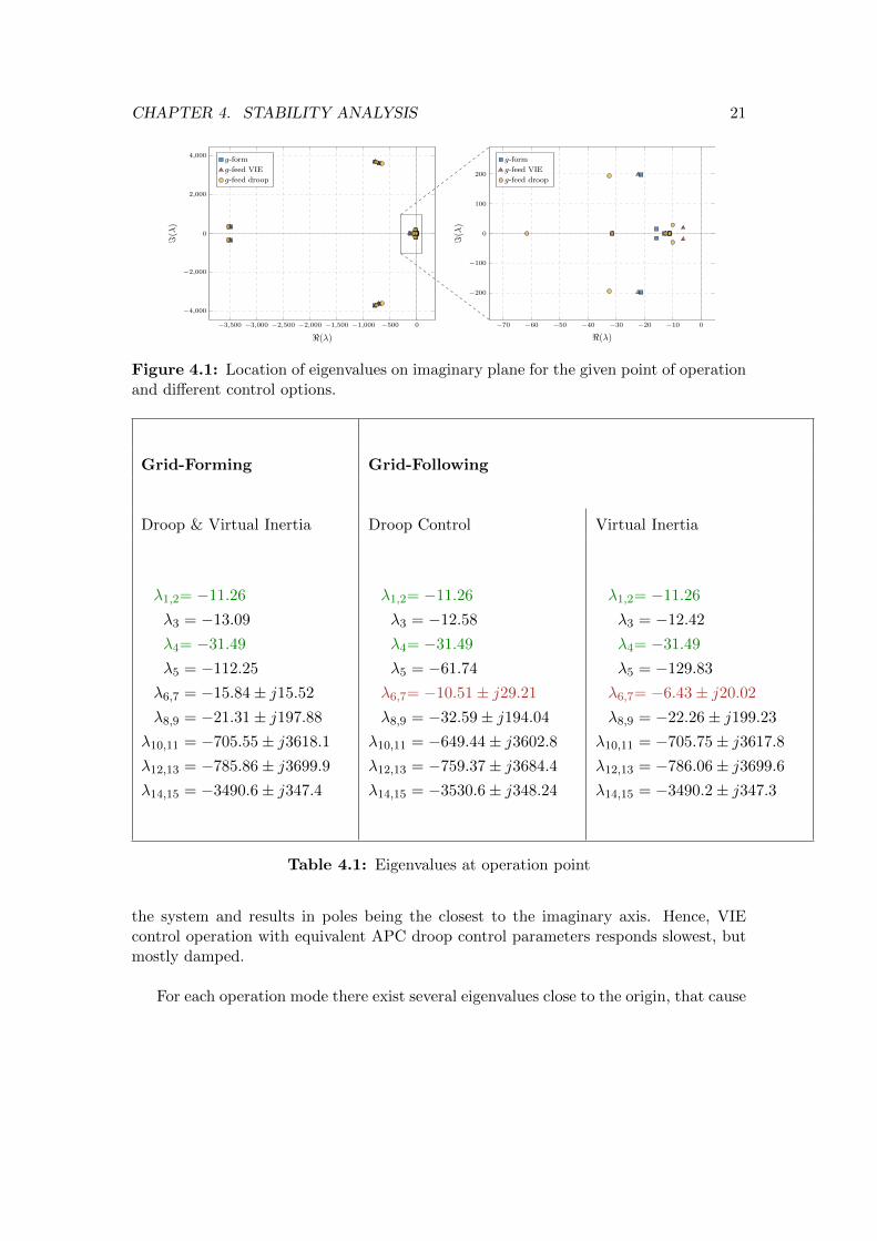
4.1 Eigenvalues at Operation Point
A typical method to asses the stability of a state-space system is to analyze the eigen-values of its state-space matrix A. In order for a system to be stable, all eigenvalueshave to be located on the left half-plane (LHP) of the complex plane, meaning:
<(λ) ≤ 0 (4.1)
where λ is the complex pole of the system. While a pole on the imaginary axis causes anoscillating term, a pole on the LHP introduces an exponentially decaying component tothe system response. The rate of decay is determined by the location of the pole: thosefar apart from the origin result in a rapid decay.
The plot in Fig. 4.1 and Tab. 4.1 contain all 15 eigenvalues for the operation condi-tions given in Tab. 3.1 for the four distinct converter modes. First of all, the eigenvaluesin g-form operation of the converter are independent of APC configuration. Due tothe PLL unit not being active and the absence of a frequency feedback-loop in g-formoperation, the different processing of the input signal does not influence the location ofthe poles. On the other hand, the location of poles differs for g-feed operation. ThePLL-unit is active in this case and the different processes of establishing frequency set-points for the inner control loops leads different pole locations. While in the case ofAPC droop control power mismatch is used to calculate the frequency setpoint, VIEdirectly processes frequency deviation. In the latter case, inertia imposes damping to
20
CHAPTER 4. STABILITY ANALYSIS 21
−3,500 −3,000 −2,500 −2,000 −1,500 −1,000 −500 0
−4,000
−2,000
0
2,000
4,000
<(λ)
=(λ)
g-form
g-feed VIE
g-feed droop
−70 −60 −50 −40 −30 −20 −10 0
−200
−100
0
100
200
<(λ)
=(λ)
g-form
g-feed VIE
g-feed droop
Figure 4.1: Location of eigenvalues on imaginary plane for the given point of operationand different control options.
Grid-Forming Grid-Following
Droop & Virtual Inertia Droop Control Virtual Inertia
λ1,2= −11.26
λ3 = −13.09
λ4= −31.49
λ5 = −112.25
λ6,7 = −15.84± j15.52
λ8,9 = −21.31± j197.88
λ10,11 = −705.55± j3618.1
λ12,13 = −785.86± j3699.9
λ14,15 = −3490.6± j347.4
λ1,2= −11.26
λ3 = −12.58
λ4= −31.49
λ5 = −61.74
λ6,7= −10.51± j29.21
λ8,9 = −32.59± j194.04
λ10,11 = −649.44± j3602.8
λ12,13 = −759.37± j3684.4
λ14,15 = −3530.6± j348.24
λ1,2= −11.26
λ3 = −12.42
λ4= −31.49
λ5 = −129.83
λ6,7= −6.43± j20.02
λ8,9 = −22.26± j199.23
λ10,11 = −705.75± j3617.8
λ12,13 = −786.06± j3699.6
λ14,15 = −3490.2± j347.3
Table 4.1: Eigenvalues at operation point
the system and results in poles being the closest to the imaginary axis. Hence, VIEcontrol operation with equivalent APC droop control parameters responds slowest, butmostly damped.
For each operation mode there exist several eigenvalues close to the origin, that cause

CHAPTER 4. STABILITY ANALYSIS 22
poor damping. Furthermore, there are two complex-conjugate pole pairs per operationwith poor damping and high oscillation frequency (λ10 to λ13). Three poles on the realaxis, that are marked in red in Tab. 4.1, are not effected by changing converter operation.
To conclude, the system is stable for any of the four investigated operation modesat the given operating point. The critical eigenvalue λ∗, meaning the eigenvalue closestto the imaginary axis, is largest for VIE control in g-feed mode, while g-form opera-tion imposes the largest stability margin. The subsequent section analyzes the stabilitymargins for changing various control parameters.
4.2 Tuning the Power Control Loops
The impact of outer control gain parameters has been investigated by alternating reactivepower droop control gain in combination with either APC droop gain or inertia constantand damping. The subsequent sections present resulting stability maps and surfaces, aswell as their margins.
4.2.1 Active Power Droop
When varying active power droop parameters (LPF cutoff frequency ωc and droop gainDp), the simulations show no effect of filter cutoff frequency on the critical eigenvalue.Hence, for APC droop control only droop gains impose restrictions. The stability mapdepicted in Fig. 4.2 indicates that for traditional active power droops in the range ofDp ∈ [1%, 5%] all investigated VSC operation modes obtain stability. However, onlyg-form operation allows to meet potentially faster power response requirements andpreserves a stability margin for Dp > 10%. Furthermore, common reactive power droopgains around Dq = 2% do not effect stability.
0 0.1 0.2 0.3 0.4 0.50
0.2
0.4
0.6
Dp
Dq
g-form
g-feed
Figure 4.2: Stability map of different converter modes on the Dp-Dq plane. The systemis stable in the shaded region.
The stability margin, particularly the distance of the critical eigenvalue to the imag-inary axis, is illustrated in Fig. 4.3. Any set of droop gains (Dp, Dq) located above thegreen zero surface is stable. These surface plots indicate that no matter the VSC mode,

CHAPTER 4. STABILITY ANALYSIS 23
the critical eigenvalue stays close to the imaginary axis. While for g-form operation it sat-urates for Dp < 40%, there exists a clear optimum for g-feed VSC mode. The maximumstability margin in the latter case can be established with active droop gain Dp = 2.5%.Repeatedly, the surfaces presented in Fig. 4.3 emphasize there is no influence of reactivedroop on either stability or stability margins in the range of traditional parameterization.
0 0.2 0.4 0.6 0.8 1
0
0.5
1
0
25
50
75
Dp
Dq
<(λ)
0
20
40
60
(a)
0 0.2 0.4 0.6 0.8 1
0
0.5
1
0
25
50
75
Dp
Dq
<(λ)
0
20
40
60
80
(b)
Figure 4.3: Critical eigenvalue λ for (a) g-form and (b) g-feed VSC operation of APCdroop control.
To conclude, in active power droop control g-form VSCs allow for increased opera-tional flexibility in tuning the outer control parameters, in general impose larger stabilitymargins and preserve stability for high responsive converters. However, stability mar-gins for both VSC modes can be matched by optimizing the active power droop gain forg-feed operation.
4.2.2 Virtual Inertia Emulation
When alternating VIE control parameters active power control variables, inertia anddamping constants, significantly effect the movement of the critical eigenvalue. Hence,before analyzing active and reactive control parameters altogether, the first stabilityassessment investigates the requirement of inertia for stable operation.
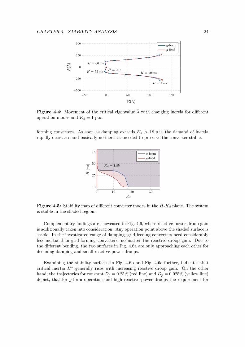
Fig. 4.4 illustrates the movement of the critical eigenvalue on the complex plane fordifferent inertia constants and converter operation, while damping is fixed to Kd = 1 p.u.As system inertia decreases below 50 ms, the critical pole pair steadily moves to the righthand side, resulting in minimum required inertia of H∗ = 40.6 ms and H∗ = 46.5 msfor g-form and g-feed operation, respectively. Again, g-form controllers obtain a higherstability margin, e.g. lower inertia requirements.
Nonetheless, this observation is only valid for damping below Kd < 1.85 p.u., as thestability map included in Fig. 4.5 suggests. For reasonable damping gain of Kd = 10 p.u.,that is equivalent to Dp = 1%, grid-feeding operation requires less inertia than grid-
CHAPTER 4. STABILITY ANALYSIS 24
−50 0 50 100 150
−500
−250
0
250
500
H = 1ms
H = 10msH = 55msH = 20 s
H = 66ms
<(λ)
=(λ)
g-form
g-feed
Figure 4.4: Movement of the critical eigenvalue λ with changing inertia for differentoperation modes and Kd = 1 p.u.
forming converters. As soon as damping exceeds Kd > 18 p.u. the demand of inertiarapidly decreases and basically no inertia is needed to preserve the converter stable.
1 10 20 30
0
25
50
75
Kd = 1.85
Kd
H[m
s]
g-form
g-feed
Figure 4.5: Stability map of different converter modes in the H-Kd plane. The systemis stable in the shaded region.
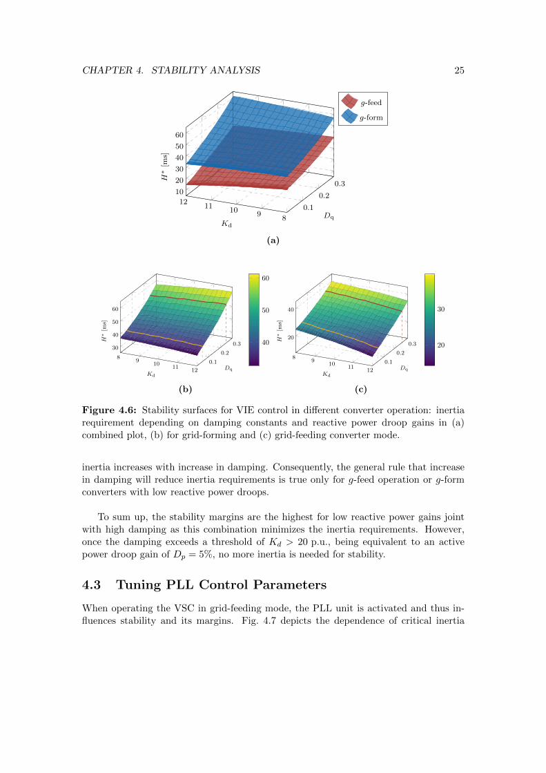
Complementary findings are showcased in Fig. 4.6, where reactive power droop gainis additionally taken into consideration. Any operation point above the shaded surface isstable. In the investigated range of damping, grid-feeding converters need considerablyless inertia than grid-forming converters, no matter the reactive droop gain. Due tothe different bending, the two surfaces in Fig. 4.6a are only approaching each other fordeclining damping and small reactive power droops.
Examining the stability surfaces in Fig. 4.6b and Fig. 4.6c further, indicates thatcritical inertia H∗ generally rises with increasing reactive droop gain. On the otherhand, the trajectories for constant Dp = 0.25% (red line) and Dp = 0.025% (yellow line)depict, that for g-form operation and high reactive power droops the requirement for
CHAPTER 4. STABILITY ANALYSIS 25
89
1011
120.1
0.2
0.310
20
30
40
50
60
Kd
Dq
H∗[m
s]
g-feed
g-form
(a)
89
1011
12
0.1
0.2
0.330
40
50
60
Kd
Dq
H∗[m
s]
40
50
60
(b)
89
1011
12
0.1
0.2
0.320
40
Kd
Dq
H∗[m
s]
20
30
(c)
Figure 4.6: Stability surfaces for VIE control in different converter operation: inertiarequirement depending on damping constants and reactive power droop gains in (a)combined plot, (b) for grid-forming and (c) grid-feeding converter mode.
inertia increases with increase in damping. Consequently, the general rule that increasein damping will reduce inertia requirements is true only for g-feed operation or g-formconverters with low reactive power droops.
To sum up, the stability margins are the highest for low reactive power gains jointwith high damping as this combination minimizes the inertia requirements. However,once the damping exceeds a threshold of Kd > 20 p.u., being equivalent to an activepower droop gain of Dp = 5%, no more inertia is needed for stability.
4.3 Tuning PLL Control Parameters
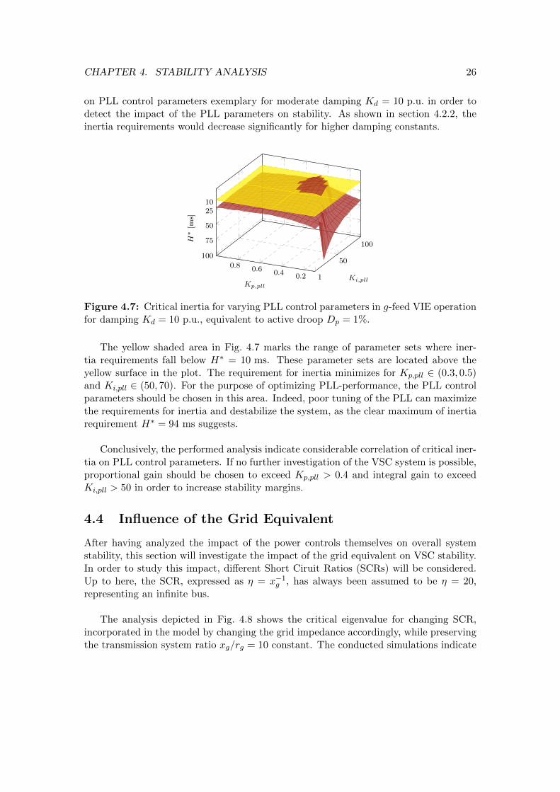
When operating the VSC in grid-feeding mode, the PLL unit is activated and thus in-fluences stability and its margins. Fig. 4.7 depicts the dependence of critical inertia
CHAPTER 4. STABILITY ANALYSIS 26
on PLL control parameters exemplary for moderate damping Kd = 10 p.u. in order todetect the impact of the PLL parameters on stability. As shown in section 4.2.2, theinertia requirements would decrease significantly for higher damping constants.
0.20.40.60.8
1
50
100
1025
50
75
100
Kp,pll
Ki,pll
H∗[m
s]
Figure 4.7: Critical inertia for varying PLL control parameters in g-feed VIE operationfor damping Kd = 10 p.u., equivalent to active droop Dp = 1%.
The yellow shaded area in Fig. 4.7 marks the range of parameter sets where iner-tia requirements fall below H∗ = 10 ms. These parameter sets are located above theyellow surface in the plot. The requirement for inertia minimizes for Kp,pll ∈ (0.3, 0.5)and Ki,pll ∈ (50, 70). For the purpose of optimizing PLL-performance, the PLL controlparameters should be chosen in this area. Indeed, poor tuning of the PLL can maximizethe requirements for inertia and destabilize the system, as the clear maximum of inertiarequirement H∗ = 94 ms suggests.
Conclusively, the performed analysis indicate considerable correlation of critical iner-tia on PLL control parameters. If no further investigation of the VSC system is possible,proportional gain should be chosen to exceed Kp,pll > 0.4 and integral gain to exceedKi,pll > 50 in order to increase stability margins.
4.4 Influence of the Grid Equivalent
After having analyzed the impact of the power controls themselves on overall systemstability, this section will investigate the impact of the grid equivalent on VSC stability.In order to study this impact, different Short Ciruit Ratios (SCRs) will be considered.Up to here, the SCR, expressed as η = x−1
g , has always been assumed to be η = 20,representing an infinite bus.
The analysis depicted in Fig. 4.8 shows the critical eigenvalue for changing SCR,incorporated in the model by changing the grid impedance accordingly, while preservingthe transmission system ratio xg/rg = 10 constant. The conducted simulations indicate
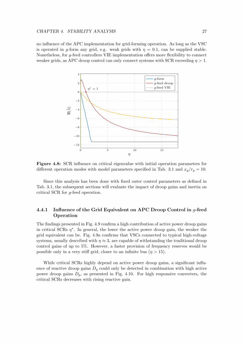
CHAPTER 4. STABILITY ANALYSIS 27
no influence of the APC implementation for grid-forming operation. As long as the VSCis operated in g-form any grid, e.g. weak grids with η = 0.1, can be supplied stable.Nonetheless, for g-feed controllers VIE implementation offers more flexibility to connectweaker grids, as APC droop control can only connect systems with SCR exceeding η > 1.
0 5 10 15
−12
−10
−8
−6
−4
−2
0
2
4
η∗ = 1
η
<(λ)
g-form
g-feed droop
g-feed VIE
Figure 4.8: SCR influence on critical eigenvalue with initial operation parameters fordifferent operation modes with model parameters specified in Tab. 3.1 and xg/rg = 10.
Since this analysis has been done with fixed outer control parameters as defined inTab. 3.1, the subsequent sections will evaluate the impact of droop gains and inertia oncritical SCR for g-feed operation.
4.4.1 Influence of the Grid Equivalent on APC Droop Control in g-feedOperation
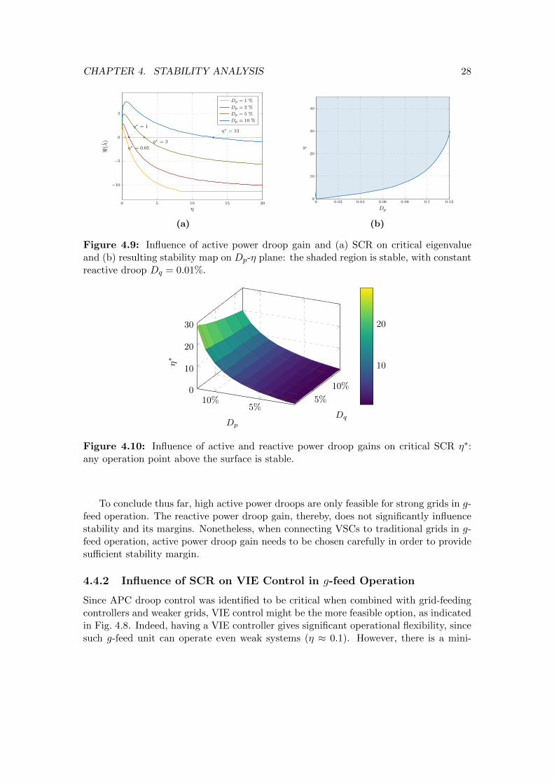
The findings presented in Fig. 4.9 confirm a high contribution of active power droop gainsin critical SCRs η∗. In general, the lower the active power droop gain, the weaker thegrid equivalent can be. Fig. 4.9a confirms that VSCs connected to typical high-voltagesystems, usually described with η ≈ 3, are capable of withstanding the traditional droopcontrol gains of up to 5%. However, a faster provision of frequency reserves would bepossible only in a very stiff grid, closer to an infinite bus (η > 15).
While critical SCRs highly depend on active power droop gains, a significant influ-ence of reactive droop gains Dq could only be detected in combination with high activepower droop gains Dp, as presented in Fig. 4.10. For high responsive converters, thecritical SCRs decreases with rising reactive gain.
CHAPTER 4. STABILITY ANALYSIS 28
0 5 10 15 20
−10
−5
0
5
η∗ = 0.05
η∗ = 1
η∗ = 3
η∗ = 13
η
<(λ)
Dp = 1 %
Dp = 2 %
Dp = 5 %
Dp = 10 %
(a)
0 0.02 0.04 0.06 0.08 0.1 0.120
10
20
30
40
Dp
η
(b)
Figure 4.9: Influence of active power droop gain and (a) SCR on critical eigenvalueand (b) resulting stability map on Dp-η plane: the shaded region is stable, with constantreactive droop Dq = 0.01%.
5%10% 5%
10%0
10
20
30
Dp
Dq
η∗
10
20
Figure 4.10: Influence of active and reactive power droop gains on critical SCR η∗:any operation point above the surface is stable.
To conclude thus far, high active power droops are only feasible for strong grids in g-feed operation. The reactive power droop gain, thereby, does not significantly influencestability and its margins. Nonetheless, when connecting VSCs to traditional grids in g-feed operation, active power droop gain needs to be chosen carefully in order to providesufficient stability margin.
4.4.2 Influence of SCR on VIE Control in g-feed Operation
Since APC droop control was identified to be critical when combined with grid-feedingcontrollers and weaker grids, VIE control might be the more feasible option, as indicatedin Fig. 4.8. Indeed, having a VIE controller gives significant operational flexibility, sincesuch g-feed unit can operate even weak systems (η ≈ 0.1). However, there is a mini-
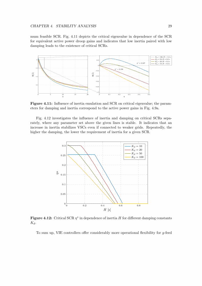
CHAPTER 4. STABILITY ANALYSIS 29
mum feasible SCR. Fig. 4.11 depicts the critical eigenvalue in dependence of the SCRfor equivalent active power droop gains and indicates that low inertia paired with lowdamping leads to the existence of critical SCRs.
0 5 10 15 20
−6
−4
−2
0
η
<(λ)
0 0.1 0.2 0.3 0.4 0.5
−1
−0.8
−0.6
−0.4
−0.2
0
0.2
η∗ = 0.196
η∗ = 0.347
η
<(λ)
Kd = 100, H = 1.6 s
Kd = 50, H = 0.8 s
Kd = 20, H = 0.3 s
Kd = 10, H = 0.2 s
Figure 4.11: Influence of inertia emulation and SCR on critical eigenvalue; the param-eters for damping and inertia correspond to the active power gains in Fig. 4.9a.
Fig. 4.12 investigates the influence of inertia and damping on critical SCRs sepa-rately, where any parameter set above the given lines is stable. It indicates that anincrease in inertia stabilizes VSCs even if connected to weaker grids. Repeatedly, thehigher the damping, the lower the requirement of inertia for a given SCR.
0 0.2 0.4 0.6 0.80
0.05
0.1
0.15
0.2
0.25
0.3
H [s]
η∗
Kd = 10
Kd = 20
Kd = 50
Kd = 100
Figure 4.12: Critical SCR η∗ in dependence of inertiaH for different damping constantsKd.
To sum up, VIE controllers offer considerably more operational flexibility for g-feed

CHAPTER 4. STABILITY ANALYSIS 30
converters. Nonetheless, when the virtual inertia is low and the VSC is connected to aweak grid, a significant amount of damping is required to ensure stable operation andprovide sufficient stability margin.

Chapter 5
Outlook and Conclusion
In this project, a detailed DAE model of a VSC was presented, including outer con-trol, inner control and a PLL. This model was linearized in order to apply small-signalstability analysis techniques and then implemented in MATLAB. Once, the DAE andsmall-signal models were validated for the full range of operation, eigenvalue analysisand various bifurcation studies were conducted. Both grid-forming and grid-feeding con-cepts have been considered, together with different active power control configurationsbased on droop and VIE control.
It was shown that the stability margins of proposed operation modes can vary sig-nificantly with respect to parameter sensitivity and robustness. In general, grid-formingconverters have shown larger stability margins and were identified to react less sensitiveto changing parameters for both active power droop and VIE control. In the case ofhigh-responsive converters with large active droop gains, grid-feeding converters face alack of stability margin and might not be able to preserve stable operation. On theother hand, VIE controlled grid-forming converters were shown to require more inertiafor realistic damping. However, the inertia requirements were small for both frequencyconfigurations.
In addition, the PLL control parameters were shown to significantly influence inertiarequirements and stability margins. Furthermore, the strength of the grid equivalent canimpose constraints on the optimal tuning of converters, especially in case of a droop-based grid-feeding unit. VIE controllers offer considerably more operational flexibility ingrid-feeding operation and retain stable even for weak grids. Nonetheless, when virtualinertia is low a significant amount of damping is required.
As all of the presented analyses were conducted for a single converter connected toa grid equivalent, future work should focus an multi-converter systems and the potentialinteraction between them, as well as the stability in presence of conventional synchronousmachines.
31
Bibliography
[1] A. Ulbig, T. S. Borsche, and G. Andersson, “Impact of Low Rotational Inertia onPower System Stability and Operation,” ArXiv e-prints, Dec. 2013.
[2] S. D’Arco, J. A. Suul, and O. B. Fosso, “Control system tuning and stability analysisof virtual synchronous machines,” in 2013 IEEE Energy Conversion Congress andExposition, Sept 2013.
[3] S. D’Arco, J. A. Suul, and O. B. Fosso, “Small-signal modelling and parametricsensitivity of a virtual synchronous machine,” in 2014 Power Systems ComputationConference, Aug 2014.
[4] S. D’Arco, J. A. Suul, and O. B. Fosso, “A virtual synchronous machine implemen-tation for distributed control of power converters in smartgrids,” Electric PowerSystems Research, vol. 122, pp. 180–197, 2015.
[5] N. Pogaku, M. Prodanovic, and T. C. Green, “Modeling, analysis and testing of au-tonomous operation of an inverter-based microgrid,” IEEE Transactions on PowerElectronics, vol. 22, pp. 613–625, March 2007.
[6] T. Green and M. Prodanovic, “Control of inverter-based micro-grids,” ElectricPower Systems Research, vol. 77, no. 9, pp. 1204 – 1213, 2007.
[7] J. Rocabert, A. Luna, F. Blaabjerg, and P. Rodrguez, “Control of power convertersin ac microgrids,” IEEE Trans. Power Electron., vol. 27, pp. 4734–4749, Nov 2012.
[8] R. Ofir, U. Markovic, P. Aristidou, and G.Hug, “Droop vs. virtual inertia: Compar-ison from the perspective of converter operation mode,” in 2018 IEEE InternationalEnergy Conference (ENERGYCON), June 2018.
[9] U. Markovic, O. Stanojev, P. Aristidou, and G. Hug, “Partial grid forming conceptfor 100% inverter-based transmission systems,” in 2018 IEEE Power and EnergySociety General Meeting (PESGM), Aug 2018.
[10] H. P. Beck and R. Hesse, “Virtual synchronous machine,” in 2007 9th InternationalConference on Electrical Power Quality and Utilisation, Oct 2007.
32

BIBLIOGRAPHY 33
[11] J. Driesen and K. Visscher, “Virtual synchronous generators,” in 2008 IEEE Powerand Energy Society General Meeting - Conversion and Delivery of Electrical Energyin the 21st Century, July 2008.
[12] X. Wang, Y. W. Li, F. Blaabjerg, and P. C. Loh, “Virtual-impedance-based controlfor voltage-source and current-source converters,” IEEE Transactions on PowerElectronics, vol. 30, pp. 7019–7037, Dec 2015.
[13] S. D’Arco, J. A. Suul, and O. B. Fosso, “Virtual synchronous machines - clas-sification of implementations and analysis of equivalence to droop controllers formicrogrids,” in 2013 IEEE Grenoble Conference, June 2013.
[14] J. C. Vasquez, J. M. Guerrero, A. Luna, P. Rodriguez, and R. Teodorescu,“Adaptive droop control applied to voltage-source inverters operating in grid-connected and islanded modes,” IEEE Transactions on Industrial Electronics,vol. 56, pp. 4088–4096, Oct 2009.
[15] S.-K. Chung, “A phase tracking system for three phase utility interface inverters,”vol. 15, no. 3, pp. 431–438.
[16] “Solve differential algebraic equations (daes) - matlab & simulink -mathworks switzerland.” https://ch.mathworks.com/help/symbolic/
solve-differential-algebraic-equations.html. (Accessed on 02/22/2018).
[17] “Solve daes using mass matrix solvers - matlab & simulink - math-works switzerland.” https://ch.mathworks.com/help/symbolic/
solve-daes-using-mass-matrix-solvers.html. (Accessed on 02/22/2018).
[18] “Linearize non-linear system using matlab/simulink.”https://ch.mathworks.com/matlabcentral/answers/
56183-linearize-non-linear-system-using-matlab-simulink. (Accessedon 02/27/2018).
[19] S. D’Arco and J. A. Suul, “Equivalence of virtual synchronous machines andfrequency-droops for converter-based microgrids,” IEEE Transactions on SmartGrid, vol. 5, no. 1, pp. 394–395, 2014.