static analysis of power systems - diva1077225/fulltext01.pdf · static analysis of power systems...
TRANSCRIPT

Static Analysisof
Power Systems
Lennart Soder
Electric Power SystemsRoyal Institute of Technology
August 2004

ii

Contents
Preface to third English edition vii
1 Introduction 1
2 Power system design 3
2.1 The development of the Swedish power system . . . . . . . . . . . . . . . . . 3
2.2 The structure of the electric power system . . . . . . . . . . . . . . . . . . . 5
3 Alternating voltage 9
3.1 Single-phase alternating voltage . . . . . . . . . . . . . . . . . . . . . . . . . 9
3.2 Complex power . . . . . . . . . . . . . . . . . . . . . . . . . . . . . . . . . . 11
3.3 Symmetrical three-phase alternating voltage . . . . . . . . . . . . . . . . . . 14
4 Models of power system components 21
4.1 Electrical characteristic of an overhead line . . . . . . . . . . . . . . . . . . . 21
4.1.1 Resistance . . . . . . . . . . . . . . . . . . . . . . . . . . . . . . . . . 22
4.1.2 Shunt conductance . . . . . . . . . . . . . . . . . . . . . . . . . . . . 22
4.1.3 Inductance . . . . . . . . . . . . . . . . . . . . . . . . . . . . . . . . . 22
4.1.4 Shunt capacitance . . . . . . . . . . . . . . . . . . . . . . . . . . . . . 25
4.2 Model of a line . . . . . . . . . . . . . . . . . . . . . . . . . . . . . . . . . . 26
4.2.1 Short lines . . . . . . . . . . . . . . . . . . . . . . . . . . . . . . . . . 26
4.2.2 Medium long lines . . . . . . . . . . . . . . . . . . . . . . . . . . . . 27
4.3 Single-phase transformer . . . . . . . . . . . . . . . . . . . . . . . . . . . . . 28
4.4 Three-phase transformer . . . . . . . . . . . . . . . . . . . . . . . . . . . . . 30
iii

iv Contents
5 Important theorems in power system analysis 31
5.1 Bus analysis, admittance matrices . . . . . . . . . . . . . . . . . . . . . . . 31
5.2 Millman’s theorem . . . . . . . . . . . . . . . . . . . . . . . . . . . . . . . . 34
5.3 Superposition theorem . . . . . . . . . . . . . . . . . . . . . . . . . . . . . . 36
5.4 Reciprocity theorem . . . . . . . . . . . . . . . . . . . . . . . . . . . . . . . 37
5.5 Thevenin-Helmholtz’ theorem . . . . . . . . . . . . . . . . . . . . . . . . . . 38
6 Analysis of symmetric three-phase systems 41
6.1 Single-line diagram and impedance network . . . . . . . . . . . . . . . . . . 43
6.2 Per-unit (pu) system . . . . . . . . . . . . . . . . . . . . . . . . . . . . . . . 44
6.2.1 Per-unit representation of transformers . . . . . . . . . . . . . . . . . 45
6.2.2 Calculations by using the per-unit system . . . . . . . . . . . . . . . 47
7 Power transmission to impedance loads 51
7.1 Twoport theory . . . . . . . . . . . . . . . . . . . . . . . . . . . . . . . . . . 51
7.1.1 Symmetrical twoports . . . . . . . . . . . . . . . . . . . . . . . . . . 52
7.2 Model of a power transmission line . . . . . . . . . . . . . . . . . . . . . . . 53
7.2.1 Model of simplified line and transformer . . . . . . . . . . . . . . . . 55
7.2.2 Connection to network . . . . . . . . . . . . . . . . . . . . . . . . . . 55
7.3 General method of calculations of symmetrical three-phase system with impedanceloads . . . . . . . . . . . . . . . . . . . . . . . . . . . . . . . . . . . . . . . 59
7.4 Extended method to be used for power loads . . . . . . . . . . . . . . . . . . 66
8 Non-linear static analysis 71
8.1 Power flow on a line . . . . . . . . . . . . . . . . . . . . . . . . . . . . . . . 71
8.1.1 Line model with rectangular series impedance . . . . . . . . . . . . . 71
8.1.2 Losses on a line . . . . . . . . . . . . . . . . . . . . . . . . . . . . . 74
8.1.3 Shunt capacitors and shunt reactors . . . . . . . . . . . . . . . . . . . 75
8.1.4 Series capacitors . . . . . . . . . . . . . . . . . . . . . . . . . . . . . 76
8.2 Power flow calculations in a network - load flow . . . . . . . . . . . . . . . . 76
8.3 Load flow for a line . . . . . . . . . . . . . . . . . . . . . . . . . . . . . . . . 80
Contents v
8.3.1 Slack bus + PU-bus . . . . . . . . . . . . . . . . . . . . . . . . . . . 81
8.3.2 Slack bus + PQ-bus . . . . . . . . . . . . . . . . . . . . . . . . . . . 81
8.4 Newton-Raphson method . . . . . . . . . . . . . . . . . . . . . . . . . . . . . 85
8.4.1 Theory . . . . . . . . . . . . . . . . . . . . . . . . . . . . . . . . . . . 85
8.4.2 Application to power systems . . . . . . . . . . . . . . . . . . . . . . 89
8.4.3 Newton-Raphson method for load flow solution . . . . . . . . . . . . 92
9 Analysis of three-phase systems using linear transformations 99
9.1 Linear transformations . . . . . . . . . . . . . . . . . . . . . . . . . . . . . . 100
9.1.1 Power invarians . . . . . . . . . . . . . . . . . . . . . . . . . . . . . 100
9.1.2 The coefficient matrix in the original space . . . . . . . . . . . . . . . 101
9.1.3 The coefficient matrix in the image space . . . . . . . . . . . . . . . . 102
9.2 Examples of linear transformations that are used in analysis of three-phasesystems . . . . . . . . . . . . . . . . . . . . . . . . . . . . . . . . . . . . . . 103
9.2.1 Symmetrical components . . . . . . . . . . . . . . . . . . . . . . . . . 103
9.2.2 Clarke’s components . . . . . . . . . . . . . . . . . . . . . . . . . . . 105
9.2.3 Park’s transformation . . . . . . . . . . . . . . . . . . . . . . . . . . . 106
9.2.4 Phasor components . . . . . . . . . . . . . . . . . . . . . . . . . . . . 107
10 Symmetrical components 111
10.1 Definitions . . . . . . . . . . . . . . . . . . . . . . . . . . . . . . . . . . . . . 111
10.2 Power calculations in un-symmetrical conditions . . . . . . . . . . . . . . . 114
11 Line model for un-symmetric three-phase conditions 117
11.1 Series impedance of single-phase overhead line . . . . . . . . . . . . . . . . . 117
11.2 Series impedance of a three-phase overhead line . . . . . . . . . . . . . . . . 118
11.2.1 Symmetrical components of the series impedance of a three-phase line 120
11.2.2 Equivalent diagram of the series impedance of a line . . . . . . . . . . 121
11.3 Shunt capacitance of a three-phase line . . . . . . . . . . . . . . . . . . . . . 124
12 Transformer model in un-symmetric three-phase conditions 127

vi Contents
13 Analysis of un-symmetric three-phase systems 131
13.1 Load modeling in the analysis of un-symmetric conditions . . . . . . . . . . 131
13.2 Connection to a system in un-symmetric conditions . . . . . . . . . . . . . . 132
13.3 Single-phase short circuit to ground . . . . . . . . . . . . . . . . . . . . . . . 133
13.4 Analysis of a network with one un-symmetrical load . . . . . . . . . . . . . . 135
13.5 General method of analysis in systems havingimpedance loads of which one is un-symmetrical . . . . . . . . . . . . . . . 140
14 Power system harmonics 153
A MATLAB-codes for Examples 7.2, 7.3, 13.2 and 13.3 159
B Matlab-codes for Example 8.10 167
C Matlab-codes for Example 8.12 169

Preface to third English edition
The first Swedish edition of this compendia was written during the summer 1991. Thecompendia has since then been used in different courses at the Department of Electric PowerEngineering at the Royal Institute of Technology in Stockholm, at the Universities of Luleaand Kalmar, and at ABB T&D University.
The author wants to acknowledge professor Goran Andersson, all graduate and undergrad-uate students and teachers in Lulea and Kalmar for all valuable comments and suggestionsto improvements and extensions.
A special acknowledge to Dr. Stefan Arnborg for his excellent translation from Swedish toEnglish.
Lennart Soder
vii

viii Preface to third English edition

Chapter 1
Introduction
In this compendium, models and mathematical methods for static analysis of power systemsare discussed.
In chapter 2, the design of the power system is described and in chapter 3, the fundamentaltheory of alternating current is presented. Models of overhead power lines and transformersare given in chapter 4, and in chapter 5 some important theorems in three-phase analysisare discussed. In chapter 6 and 7, power system calculations in symmetrical conditions areperformed by using the theorems presented earlier.
Chapter 5–7 are based on the assumption that the power system loads can be modeled asimpedance loads. This leads to a linear formulation of the problem, and by that, relativelyeasy forms of solution methods can be used. In some situations, it is more accurate to modelthe system loads as power loads. How the system analysis should be carried out in suchconditions is elaborated on in chapter 8.
In chapter 9, an overview of linear transformations in order to simplify the power systemanalysis, is given. In chapter 10–13, the basic concepts of analysis in un-symmetrical con-ditions are given. The use of symmetrical components is presented in detail in chapter 10.The modeling of lines, cables and transformers must be more detailed in un-symmetricalconditions, this is the topic of chapter 11–12. In chapter 13, an un-symmetrical, three-phasepower system with impedance loads is analyzed.
In chapter 3–13, it is assumed that the power system frequency is constant and the systemcomponents are linear, i.e. sinusoidal voltages gives sinusoidal currents. With non-linearcomponents in the system, as high power electronic devices, non-sinusoidal currents andvoltages will appear. The consequences such non-sinusoidal properties can have on thepower system will be discussed briefly in chapter 14.
1

2 1. Introduction
Chapter 2
Power system design
2.1 The development of the Swedish power system
The Swedish power system started to develop around a number of hydro power stations,Porjus in Norrland, Alvkarleby in eastern Svealand, Motala in the middle of Svealand andTrollhattan in Gotaland, at the time of the first world war. Later on, coal fired powerplants located at larger cities as Stockholm, Goteborg, Malmo and Vasteras came into oper-ation. At the time for the second world war, a comprehensive proposal was made concerningexploitation of the rivers in the northern part of Sweden. To transmit this power to themiddle and south parts of Sweden, where the heavy metal industry were located, a 220 kVtransmission system was planned.
Today, the transmission system is well developed with a nominal voltage of 220 or 400 kV.In rough outline, the transmission system consists of lines, transformers and sub-stations.
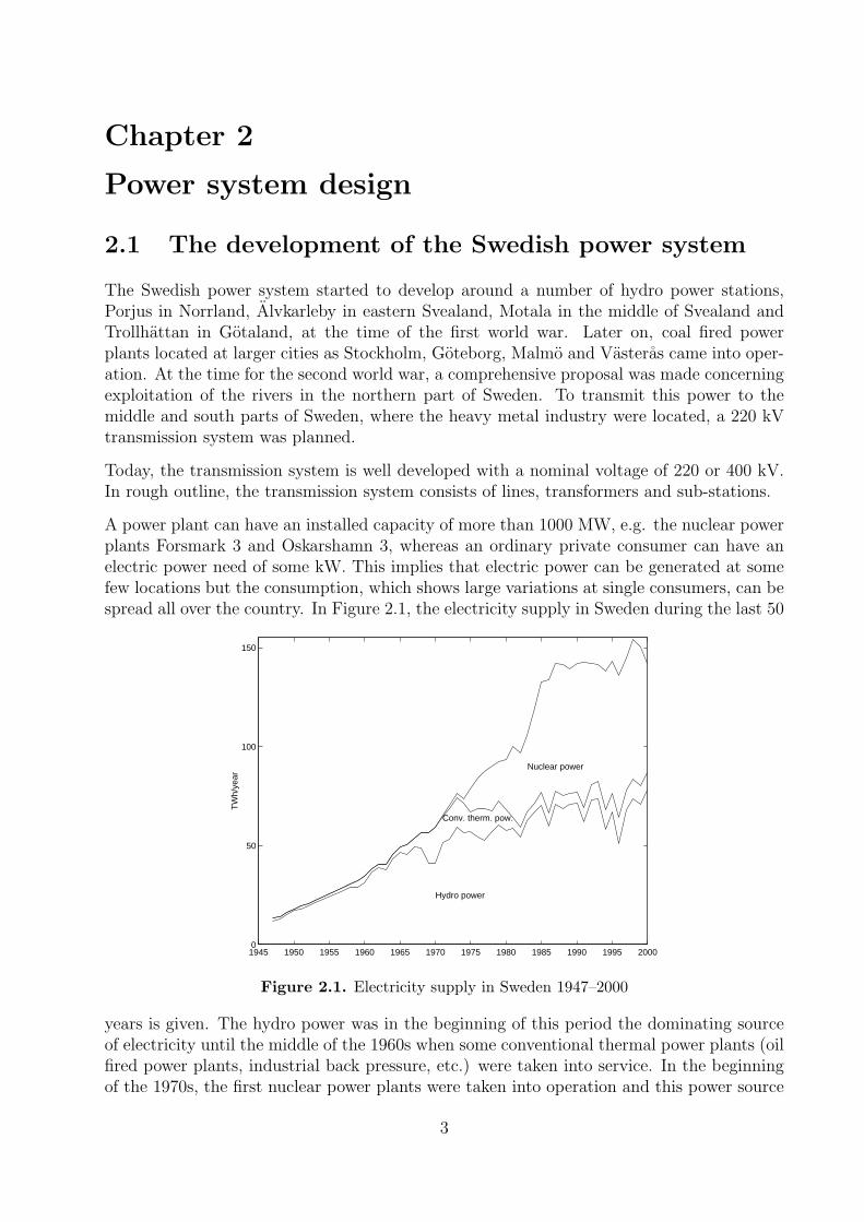
A power plant can have an installed capacity of more than 1000 MW, e.g. the nuclear powerplants Forsmark 3 and Oskarshamn 3, whereas an ordinary private consumer can have anelectric power need of some kW. This implies that electric power can be generated at somefew locations but the consumption, which shows large variations at single consumers, can bespread all over the country. In Figure 2.1, the electricity supply in Sweden during the last 50
1945 1950 1955 1960 1965 1970 1975 1980 1985 1990 1995 20000
50
100
150
TW
h/ye
ar
Hydro power
Conv. therm. pow.
Nuclear power
Figure 2.1. Electricity supply in Sweden 1947–2000
years is given. The hydro power was in the beginning of this period the dominating sourceof electricity until the middle of the 1960s when some conventional thermal power plants (oilfired power plants, industrial back pressure, etc.) were taken into service. In the beginningof the 1970s, the first nuclear power plants were taken into operation and this power source
3
4 2. Power system design
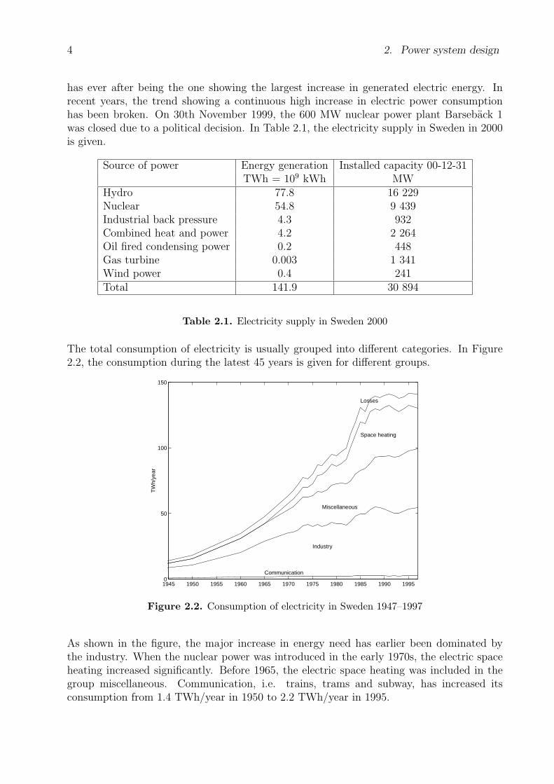
has ever after being the one showing the largest increase in generated electric energy. Inrecent years, the trend showing a continuous high increase in electric power consumptionhas been broken. On 30th November 1999, the 600 MW nuclear power plant Barseback 1was closed due to a political decision. In Table 2.1, the electricity supply in Sweden in 2000is given.
Source of power Energy generation Installed capacity 00-12-31TWh = 109 kWh MW
Hydro 77.8 16 229Nuclear 54.8 9 439Industrial back pressure 4.3 932Combined heat and power 4.2 2 264Oil fired condensing power 0.2 448Gas turbine 0.003 1 341Wind power 0.4 241Total 141.9 30 894
Table 2.1. Electricity supply in Sweden 2000
The total consumption of electricity is usually grouped into different categories. In Figure2.2, the consumption during the latest 45 years is given for different groups.
1945 1950 1955 1960 1965 1970 1975 1980 1985 1990 19950
50
100
150
TW
h/ye
ar
Communication
Industry
Miscellaneous
Space heating
Losses
Figure 2.2. Consumption of electricity in Sweden 1947–1997
As shown in the figure, the major increase in energy need has earlier been dominated bythe industry. When the nuclear power was introduced in the early 1970s, the electric spaceheating increased significantly. Before 1965, the electric space heating was included in thegroup miscellaneous. Communication, i.e. trains, trams and subway, has increased itsconsumption from 1.4 TWh/year in 1950 to 2.2 TWh/year in 1995.
2.2. The structure of the electric power system 5
In proportion to the total electricity consumption, the communication group has decreasedfrom 7.4 % to 1.6 % during the same period. The losses on the transmission and distri-bution systems have during the period 1950–1995 decreased from more than 10 % of totalconsumption to approximately 7 %.
2.2 The structure of the electric power system
A power system consist of generation sources which via power lines and transformers trans-mits the electric power to the end consumers.
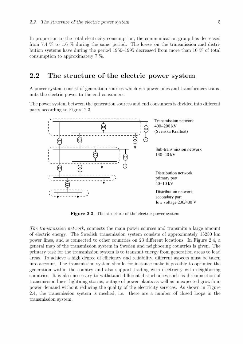
The power system between the generation sources and end consumers is divided into differentparts according to Figure 2.3.
~
~
Transmission network
400−200 kV
(Svenska Kraftnät)
Subtransmission network
130−40 kV
Distribution networkprimary part
40−10 kV
Distribution network
secondary part
low voltage 230/400 V
Figure 2.3. The structure of the electric power system
The transmission network, connects the main power sources and transmits a large amountof electric energy. The Swedish transmission system consists of approximately 15250 kmpower lines, and is connected to other countries on 23 different locations. In Figure 2.4, ageneral map of the transmission system in Sweden and neighboring countries is given. Theprimary task for the transmission system is to transmit energy from generation areas to loadareas. To achieve a high degree of efficiency and reliability, different aspects must be takeninto account. The transmission system should for instance make it possible to optimize thegeneration within the country and also support trading with electricity with neighboringcountries. It is also necessary to withstand different disturbances such as disconnection oftransmission lines, lightning storms, outage of power plants as well as unexpected growth inpower demand without reducing the quality of the electricity services. As shown in Figure2.4, the transmission system is meshed, i.e. there are a number of closed loops in thetransmission system.

6 2. Power system design
Figure 2.4. Transmission system in north-western Europe
A new state utility, Svenska Kraftnat, was launched on January 1, 1992, to manage thenational transmission system and foreign links in operation at date. Svenska Kraftnat ownsall 400 kV lines, all transformers between 400 and 220 kV and the major part of the 220 kVlines in Sweden. Note that the Baltic Cable between Sweden and Germany was taken intooperation after the day Svenska Kraftnat was launched and is therefore not owned by them.
Sub-transmission network, in Sweden also called regional network, has in each load region thesame or partly the same purpose as the transmission network. The amount of energy trans-mitted and the transmission distance are smaller compared with the transmission networkwhich gives that technical-economical constraints implies lower system voltages. Regionalnetworks are usually connected to the transmission network at two locations.
Distribution network, transmits and distributes the electric power that is taken from the sub-stations in the sub-transmission network and delivers it to the end users. The distributionnetwork is in normal operation a radial network, i.e. there is only one path from the sub-transmission sub-station to the end user.
2.2. The structure of the electric power system 7
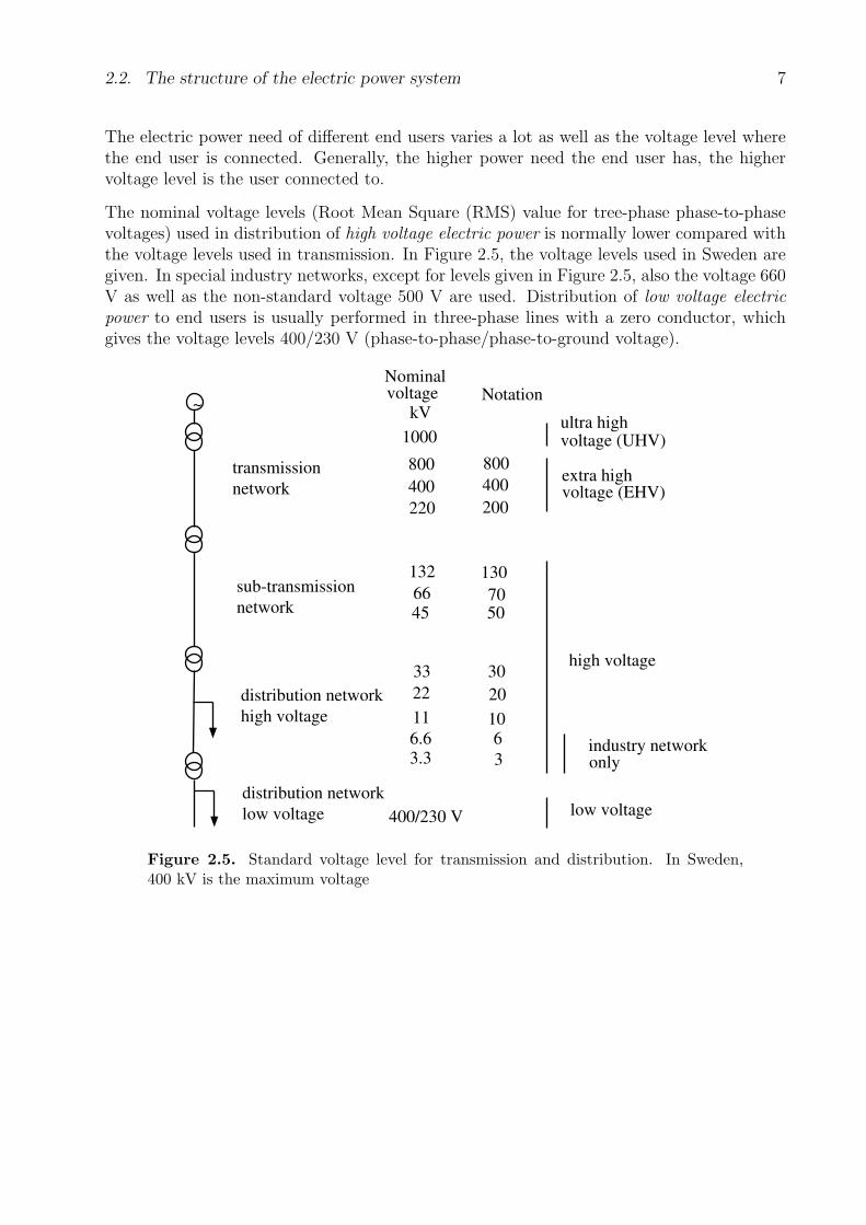
The electric power need of different end users varies a lot as well as the voltage level wherethe end user is connected. Generally, the higher power need the end user has, the highervoltage level is the user connected to.
The nominal voltage levels (Root Mean Square (RMS) value for tree-phase phase-to-phasevoltages) used in distribution of high voltage electric power is normally lower compared withthe voltage levels used in transmission. In Figure 2.5, the voltage levels used in Sweden aregiven. In special industry networks, except for levels given in Figure 2.5, also the voltage 660V as well as the non-standard voltage 500 V are used. Distribution of low voltage electricpower to end users is usually performed in three-phase lines with a zero conductor, whichgives the voltage levels 400/230 V (phase-to-phase/phase-to-ground voltage).
~
transmission
network
subtransmission
network
distribution network
high voltage
distribution network
low voltage 400/230 V
33
22
11
6.63.3
30
20
106
3
132
6645
130
7050
1000
800
400
220
800
400
200
Nominalvoltage
kVNotation
ultra highvoltage (UHV)
extra highvoltage (EHV)
high voltage
low voltage
industry networkonly
Figure 2.5. Standard voltage level for transmission and distribution. In Sweden,400 kV is the maximum voltage

8 2. Power system design
Chapter 3
Alternating voltage
In this chapter, the fundamental properties of alternating voltage, alternating current andpower under symmetrical conditions are summarized.
3.1 Single-phase alternating voltage
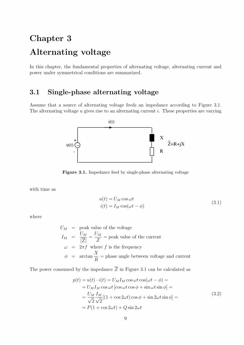
Assume that a source of alternating voltage feeds an impedance according to Figure 3.1.The alternating voltage u gives rise to an alternating current i. These properties are varying
X
R
i(t)
+
u(t) Z=R+jX~
Figure 3.1. Impedance feed by single-phase alternating voltage
with time as
u(t) = UM cos ωt
i(t) = IM cos(ωt− φ)(3.1)
where
UM = peak value of the voltage
IM =UM
|Z| =UM
Z= peak value of the current
ω = 2πf where f is the frequency
φ = arctanX
R= phase angle between voltage and current
The power consumed by the impedance Z in Figure 3.1 can be calculated as
p(t) = u(t) · i(t) = UMIM cos ωt cos(ωt− φ) =
= UMIM cos ωt [cos ωt cos φ + sin ωt sin φ] =
=UM√
2
IM√2[(1 + cos 2ωt) cos φ + sin 2ωt sin φ] =
= P (1 + cos 2ωt) + Q sin 2ωt
(3.2)
9
10 3. Alternating voltage
where
P =UM√
2
IM√2
cos φ = active power
Q =UM√
2
IM√2
sin φ = reactive power
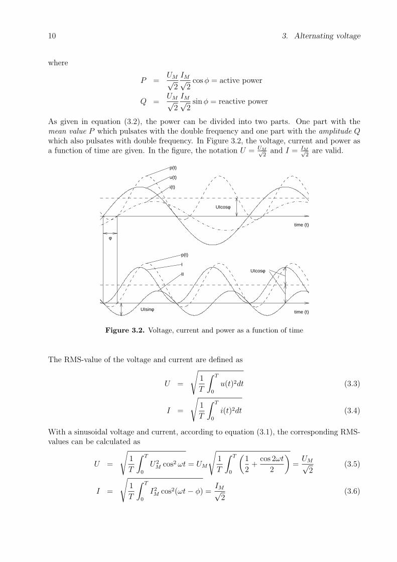
As given in equation (3.2), the power can be divided into two parts. One part with themean value P which pulsates with the double frequency and one part with the amplitude Qwhich also pulsates with double frequency. In Figure 3.2, the voltage, current and power asa function of time are given. In the figure, the notation U = UM√
2and I = IM√
2are valid.
time (t)
i(t)
u(t)
p(t)
UIcosφ
p(t)
time (t)
I
II
UIsinφ
UIcosφ
φ
Figure 3.2. Voltage, current and power as a function of time
The RMS-value of the voltage and current are defined as
U =
√1
T
∫ T
0
u(t)2dt (3.3)
I =
√1
T
∫ T
0
i(t)2dt (3.4)
With a sinusoidal voltage and current, according to equation (3.1), the corresponding RMS-values can be calculated as
U =
√1
T
∫ T
0
U2M cos2 ωt = UM
√1
T
∫ T
0
(1
2+
cos 2ωt
2
)=
UM√2
(3.5)
I =
√1
T
∫ T
0
I2M cos2(ωt− φ) =
IM√2
(3.6)
3.2. Complex power 11
Example 3.1 Which mean power is consumed by a resistor of 1210 Ω which is fed by analternating voltage of 50 Hz and 220 V RMS.
Solution
The power consumed in the resistor can be calculated as the time mean value during oneperiod as
P =1
T
∫ T
0
R · i2(t)dt =1
T
∫ T
0
Ru2(t)
R2dt =
1
R
1
T
∫ T
0
u2(t)dt
which can be rewritten according to equation (3.3) as
P =1
RU2 =
2202
1210= 40 W
3.2 Complex power
The complex method is a powerful tool for calculation of electrical power and can offersolutions in an elegant manner.
The complex single-phase voltage and current can be expressed as
U = Uej arg(U)
I = Iej arg(I)(3.7)
where
U = complex voltage
U = UM/√
2 = voltage RMS-value
I = complex current
I = IM/√
2 = current RMS-value
The complex power is defined as
S = Sej arg(S) = P + jQ = UI∗
= UIej(arg(U)−arg(I)) (3.8)
where
S = complex power
With phase angles on the voltage and the current as given in equation (3.1), i.e. arg(U) = 0and arg(I) = −φ, together with equation (3.8) the result is
S = P + jQ = UI∗
= UIejφ = UI(cos φ + j sin φ) (3.9)
which implies that
P = S cos φ = UI cos φ
Q = S sin φ = UI sin φ(3.10)
i.e. P = active power and Q = reactive power.
12 3. Alternating voltage
Example 3.2 Calculate the power consumed by an inductor rated 3.85 H which is fed by asinusoidal voltage with 50 Hz and 220 V RMS.
Solution
The impedance of the inductor can be calculated as
Z = jωL = j · 2 · π · 50 · 3.85 = j1210 Ω
The complex current through the inductor can be calculated as
I =U
Z=
220
j1210= −j0.1818 A
giving that the complex power can be calculates as
S = UI∗
= 220(−j0.1818)∗ = 220(j0.1818) = j40 VA
i.e. P = 0 W, Q = 40 VAr.
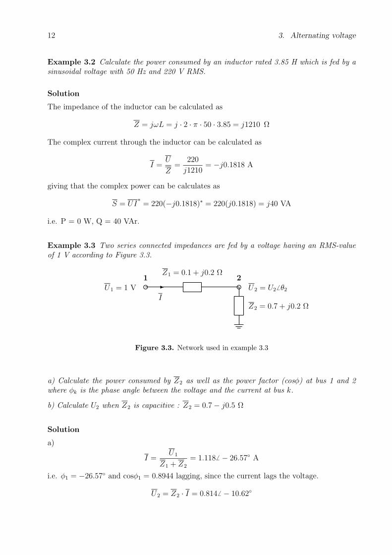
Example 3.3 Two series connected impedances are fed by a voltage having an RMS-valueof 1 V according to Figure 3.3.
e e1 2
-U1 = 1 V
I
Z1 = 0.1 + j0.2 Ω
Z2 = 0.7 + j0.2 Ω
U2 = U2 6 θ2
Figure 3.3. Network used in example 3.3
a) Calculate the power consumed by Z2 as well as the power factor (cosφ) at bus 1 and 2where φk is the phase angle between the voltage and the current at bus k.
b) Calculate U2 when Z2 is capacitive : Z2 = 0.7− j0.5 Ω
Solution
a)
I =U1
Z1 + Z2
= 1.118 6 − 26.57 A
i.e. φ1 = −26.57 and cosφ1 = 0.8944 lagging, since the current lags the voltage.
U2 = Z2 · I = 0.8146 − 10.62
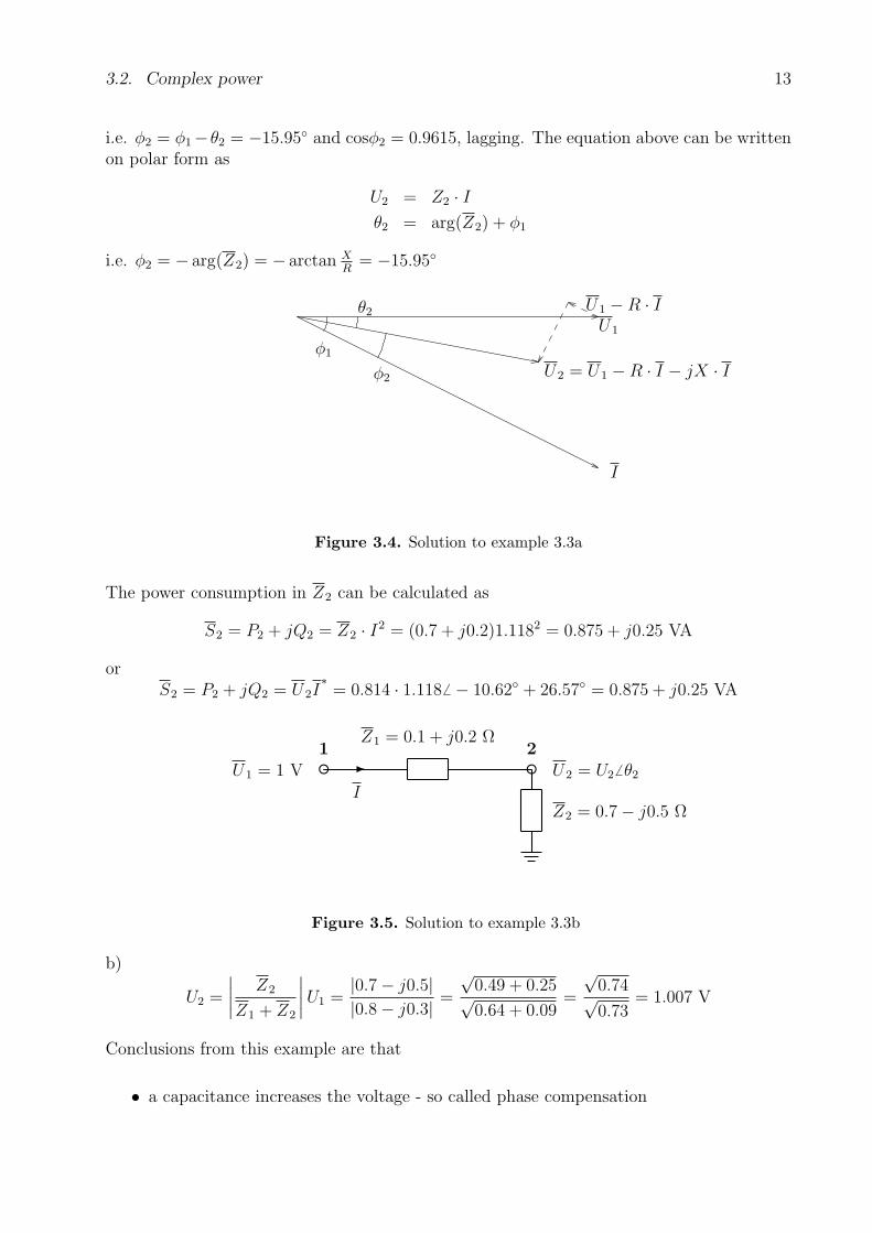
3.2. Complex power 13
i.e. φ2 = φ1−θ2 = −15.95 and cosφ2 = 0.9615, lagging. The equation above can be writtenon polar form as
U2 = Z2 · Iθ2 = arg(Z2) + φ1
i.e. φ2 = − arg(Z2) = − arctan XR
= −15.95
U1
U1 −R · I
U2 = U1 −R · I − jX · I
I
φ1
φ2
θ2
Figure 3.4. Solution to example 3.3a
The power consumption in Z2 can be calculated as
S2 = P2 + jQ2 = Z2 · I2 = (0.7 + j0.2)1.1182 = 0.875 + j0.25 VA
orS2 = P2 + jQ2 = U2I
∗= 0.814 · 1.1186 − 10.62 + 26.57 = 0.875 + j0.25 VA
e e1 2
-U1 = 1 V
I
Z1 = 0.1 + j0.2 Ω
Z2 = 0.7− j0.5 Ω
U2 = U2 6 θ2
Figure 3.5. Solution to example 3.3b
b)
U2 =
∣∣∣∣Z2
Z1 + Z2
∣∣∣∣U1 =|0.7− j0.5||0.8− j0.3| =
√0.49 + 0.25√0.64 + 0.09
=
√0.74√0.73
= 1.007 V
Conclusions from this example are that
• a capacitance increases the voltage - so called phase compensation
14 3. Alternating voltage
• active power can be sent towards higher voltage
• cosφ is different in different ends of a line
• the line impedances are ¿ load impedances
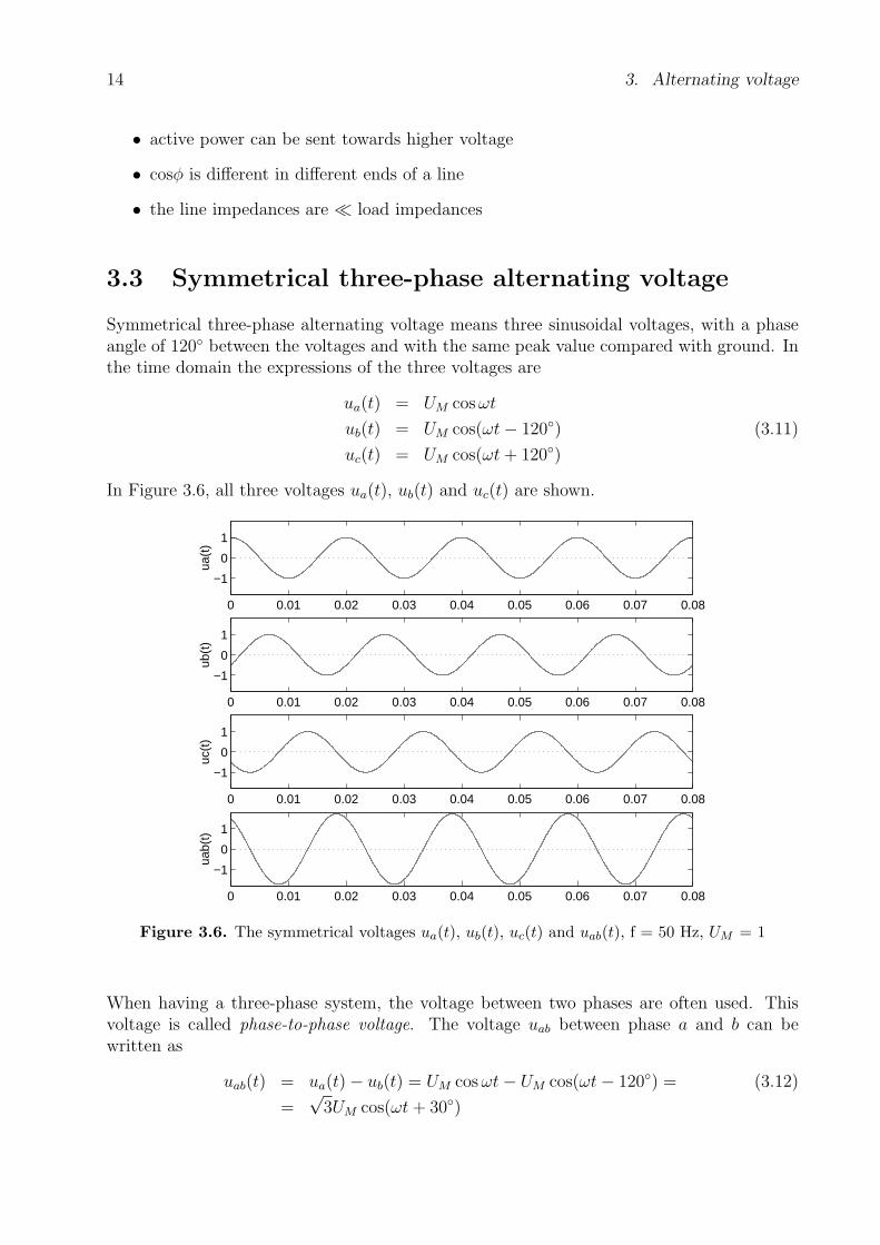
3.3 Symmetrical three-phase alternating voltage
Symmetrical three-phase alternating voltage means three sinusoidal voltages, with a phaseangle of 120 between the voltages and with the same peak value compared with ground. Inthe time domain the expressions of the three voltages are
ua(t) = UM cos ωt
ub(t) = UM cos(ωt− 120) (3.11)
uc(t) = UM cos(ωt + 120)
In Figure 3.6, all three voltages ua(t), ub(t) and uc(t) are shown.
0 0.01 0.02 0.03 0.04 0.05 0.06 0.07 0.08
−1
0
1
ua(t
)
0 0.01 0.02 0.03 0.04 0.05 0.06 0.07 0.08
−1
0
1
ub(t
)
0 0.01 0.02 0.03 0.04 0.05 0.06 0.07 0.08
−1
0
1
uc(t
)
0 0.01 0.02 0.03 0.04 0.05 0.06 0.07 0.08
−1
0
1
uab(
t)
Figure 3.6. The symmetrical voltages ua(t), ub(t), uc(t) and uab(t), f = 50 Hz, UM = 1
When having a three-phase system, the voltage between two phases are often used. Thisvoltage is called phase-to-phase voltage. The voltage uab between phase a and b can bewritten as
uab(t) = ua(t)− ub(t) = UM cos ωt− UM cos(ωt− 120) = (3.12)
=√
3UM cos(ωt + 30)

3.3. Symmetrical three-phase alternating voltage 15
i.e. the phase-to-phase voltage has an amplitude (and by that an RMS-value, see equation(3.5)) which is
√3 times larger than the amplitude of the phase voltage (phase-to-ground
voltage). An example is low voltage distribution where the RMS-value of the phase voltageis 230 V and the RMS-value of the phase-to-phase voltage is
√3 · 230 = 400 V.
Equation (3.12) shows also that uab is leading the voltage ua by 30. The phase-to-phasevoltage uab is shown at the bottom of Figure 3.6.
With the assumption that the phase angle between the voltage and the current is φ (equalin all phases because of symmetrical conditions), the following expression of the three phasecurrents can be obtained :
ia(t) = IM cos(ωt− φ)
ib(t) = IM cos(ωt− 120 − φ) (3.13)
ic(t) = IM cos(ωt + 120 − φ)
For the total symmetrical three-phase power, the following is valid :
p3(t) = pa(t) + pb(t) + pc(t) = ua(t)ia(t) + ub(t)ib(t) + uc(t)ic(t) =
=UM√
2
IM√2[(1 + cos 2ωt) cos φ + sin 2ωt sin φ] + (3.14)
+UM√
2
IM√2[(1 + cos 2[ωt− 120]) cos φ + sin 2[ωt− 120] sin φ] +
+UM√
2
IM√2[(1 + cos 2[ωt + 120]) cos φ + sin 2[ωt + 120] sin φ] =
= 3UM√
2
IM√2
[cos φ + (cos 2ωt + cos 2[ωt− 120] + cos 2[ωt + 120])︸ ︷︷ ︸
=0
+
+ (sin 2ωt + sin 2[ωt− 120] + sin 2[ωt + 120])︸ ︷︷ ︸=0
]= 3
UM√2
IM√2
cos φ
i.e. it is constant and does not pulsate as the single-phase power does. This is one veryimportant reason why the electric power usually is transmitted by a three-phase system.Corresponding complex properties of the voltages are :
Ua = Uf 6 0
U b = Uf 6 − 120 (3.15)
U c = Uf 6 120
The symmetrical voltages are shown in Figure 3.7.
In the figure also the phase-to-phase voltages Uab, U bc and U ca are indicated. These phase-to-phase voltages form together a symmetrical tree-phase system, i.e. they have the sameamplitude and are individually separated by a 120 phase angle. In the same way as for thetime domain expressions, the complex formulation of the phase-to-phase voltage Uab can bewritten as
Uab = Ua − U b = Uf (1− e−j120) =√
3Uf 6 30 (3.16)

16 3. Alternating voltage
+120o
120o
Ua
Ub
Uc
Uab
Uca
Ubc
Figure 3.7. The symmetrical voltages Ua, U b, and U c as well as the phase-to-phase voltages
where the RMS-value of the phase-to-phase voltage is√
3 times larger than the RMS-valueof the phase-to-ground voltage.
The complex expressions of the currents are :
Ia = I 6 (0 − φ)
Ib = I 6 (−120 − φ) (3.17)
Ic = I 6 (120 − φ)
and the total three-phase power :
S3 = UaI∗a + U bI
∗b + U cI
∗c = 3UfI cos φ + j3UfI sin φ =
= 3UfIejφ(3.18)
In equation (3.18), Uf is the RMS-value of the phase-to-ground voltage. If the expressionis rewritten in order to use the absolute value of the phase-to-phase voltage U =
√3Uf the
following is obtained
S3 =√
3UIejφ =√
3Uej arg(U)Ie−j(arg(U)−δ =√
3UI∗
(3.19)
When discussing a voltage in a three-phase system, e.g. 10 kV, normally it is assumed thatit is the RMS-value of the phase-to-phase voltage that is discussed. This will also apply inthis compendium. It is also common that an angle is attached to the absolute value of thephase-to-phase voltage. That angle is normally the phase-to-ground angle. This will alsoapply in this compendium.
Example 3.4 The student Elektra lives in a house situated 2 km from a transformer havinga completely symmetrical three-phase voltage (Ua = 220V 6 0, U b = 220V 6 − 120, U c =

3.3. Symmetrical three-phase alternating voltage 17
220V 6 120 ). The house is connected to this transformer via a three-phase cable (EKKJ,3×16 mm2 + 16 mm2). A cold day, Elektra switches on two electrical radiators to eachphase, each radiator is rated 1000 W (at 220 V with cosφ = 0.995 lagging (inductive)).Assume that the cable can be modeled as four impedances connected in parallel (zL = 1.15 +j0.08 Ω/phase,km, zL0 = 1.15 + j0.015 Ω/km) and that the radiators also can be consideredas impedances. Calculate the total thermal power given by the radiators.
o
o
o
o
o
o
o
o
ZL
ZL
ZL
ZL0
Za
Zb
Zc
Ib
Ic
I0
Ia
Ua
Ub
Uc
U0
U’0
U’c
U’b
U’a
Figure 3.8. Single line diagram for example
Solution
Ua = 220 6 0 V, U b = 220 6 − 120 V, U c = 220 6 120 V
ZL = 2(1.15 + j0.08) = 2.3 + j0.16 Ω
ZL0 = 2(1.15 + j0.015) = 2.3 + j0.03 Ω
Pa = Pb = Pc = 2000 W (at 220 V, cos φ = 0.995)
sin φ =√
1− cos2 φ = 0.0999
Qa = Qb = Qc = S sin φ = Pcos φ
sin φ = 200.8 VAr
Za = Zb = Zc = UI
= U ·U∗I·U∗ = U2/S
∗= U2/(Pa − jQa) = 23.96 + j2.40 Ω
Ia = Ua−U′0
ZL+ZaIb = Ub−U
′0
ZL+ZbIc = Uc−U
′0
ZL+Zc
Ia + Ib + Ic = U′0−U0
ZL0= U
′0−0
ZL0
⇒ U′0
[1
ZL0+ 1
ZL+Za+ 1
ZL+Zb+ 1
ZL+Zc
]= Ua
ZL+Za+ Ub
ZL+Zb+ Uc
ZL+Zc
⇒ U′0 = 0.0
⇒ Ia = 8.346 − 5.58 A, Ib = 8.34 6 − 125.58 A, Ic = 8.34 6 114.42 A
The voltage at the radiators can be calculated as :
U′a = U
′0 + IaZa = 200.786 0.15 V
U b = 200.78 6 − 119.85 V
U c = 200.786 120.15 V
Finally, the power to the radiators can be calculated as

18 3. Alternating voltage
Sza = ZaI2a = 1666 + j167 VA
Szb = ZbI2b = 1666 + j167 VA
Szc = ZaI2c = 1666 + j167 VA
The total amount of power consumed is
Sza + Szb + Szc = 4998 + j502 VA, i.e. the thermal power = 4998 W
The total transmission losses are
ZL(I2a + I2
b + I2c ) + ZL0|Ia + Ib + Ic|2) = 480 + j33 VA
i.e. the active losses are 480 W, which means that the efficiency is 91.2 %. As shownin example 3.4, a symmetrical voltage that feeds a symmetrical impedance gives rise to asymmetrical current. As a consequence, no current will flow in the neutral conductor. Sincethe voltage at the neutral connection point at the house = 0, it is possible to perform thecalculations one phase at the time without paying attention to the other phases. The totalamount of power consumed can be calculated as three times the power consumption perphase.
Example 3.5 Use the same example as 3.4 but with the difference that the student Elektraconnects one 1000 W radiator (at 220 V with cosφ = 0.995 lagging) to phase a, three radiatorsto phase b and two to phase c. Calculate the total thermal power given by the radiators, aswell as the system losses.
Solution
Ua = 220 6 0 V, U b = 220 6 − 120 V, U c = 220 6 120 V
ZL = 2(1.15 + j0.08) = 2.3 + j0.16 Ω
ZL0 = 2(1.15 + j0.015) = 2.3 + j0.03 Ω
Pa = 1000 W (at 220 V, cos φ = 0.995)
sin φ =√
1− cos2 φ = 0.0999
Qa = S sin φ = Pcos φ
sin φ = 100.4 VAr
Za = U2/S∗a = U2/(Pa − jQa) = 47.9 + j4.81 Ω
Zb = Za/3 = 15.97 + j1.60 Ω
Zc = Za/2 = 23.96 + j2.40 Ω
U′0
[1
ZL0+ 1
ZL+Za+ 1
ZL+Zb+ 1
ZL+Zc
]= Ua
ZL+Za+ Ub
ZL+Zb+ Uc
ZL+Zc
⇒ U′0 = 12.08 6 − 155.14 V
⇒ Ia = 4.586 − 4.39 A, Ib = 11.456 − 123.62 A, Ic = 8.316 111.28 A
The voltages at the radiators can be calculated as :
U′a = U
′0 + IaZa = 209.456 0.02 V
U′b = U
′0 + IbZb = 193.60 6 − 120.05 V

3.3. Symmetrical three-phase alternating voltage 19
U′c = U
′0 + IcZc = 200.916 129.45 V
Observe that these voltages are not local phase voltages since they are calculated as U′a−U
′0
etc. The power to the radiators can be calculated as :
Sza = ZaI2a = 1004 + j101 VA
Szb = ZbI2b = 2095 + j210 VA
Szc = ZaI2c = 1655 + j166 VA
The total amount of power consumed is
Sza + Szb + Szc = 4754 + j477 VA, i.e. the thermal power is 4754 W
The total transmission losses are
ZL(I2a + I2
b + I2c ) + ZL0|Ia + Ib + Ic|2) = 572.1 + j36 VA, i.e. 572.1 W
which gives an efficiency of 89.3 %. As shown in this example, an un-symmetrical impedancewill give an un-symmetrical current. As a consequence, a voltage can be detected in theneutral conductor which gives rise to a current in the neutral conductor. The total thermalpower obtained was reduced by approximately 5 % and the line losses increased partly dueto the losses in the neutral conductor. The efficiency of the transmission decreased. It canalso be noted that the power per radiator decreased with the number of radiators connectedto the same phase. This owing to the fact that the voltage in the neutral connection pointwill be closest to the voltage in the phase with the lowest impedance, i.e. the phase withthe largest number of radiators connected.

20 3. Alternating voltage

Chapter 4
Models of power system components
Electric energy is transmitted from power plants to consumers via overhead lines, cables andtransformers. In the following, these components will be discussed and mathematical modelsto be used in the analysis of symmetrical three-phase systems will be derived. In chapter 11and 12, analysis of power systems under un-symmetrical conditions will be discussed.
4.1 Electrical characteristic of an overhead line
Overhead transmission lines need large surface area and are mostly suitable to be used inrural areas and in areas with low population density. In areas with high population densityand urban areas cables are a better alternative. For a certain amount of power transmitted,a cable transmission system is about ten times as expensive as an overhead transmissionsystem.
Power lines have a resistance r owing to the resistivity of the conductor and a shunt conduc-tance g because of leakage currents in the insulation. The lines also have an inductance `owing to the magnetic flux surrounding the line as well as a shunt capacitance c because ofthe electric field between the lines and between the lines and ground. These quantities aregiven per unit length and are continuously distributed along the whole length of the line.Resistance and inductance are in series while the conductance and capacitance are shuntquantities.
l r
c g
l r
c g
l r
c g
l r
c g
Figure 4.1. A line with distributed quantities
Assuming symmetrical three-phase, a line can be modeled as shown in Figure 4.1. Thequantities r, g, `, and c determines the characteristics of a line. Power lines can be modeledby simple equivalent circuits which, together with models of other system components, canbe formed to a model of a complete system or parts of it. This is important since suchmodels are used in power system analysis where active and reactive power flows in thenetwork, voltage levels, losses, power system stability and other properties at disturbancesas e.g. short circuits, are of interest.
For a more detailed derivation of the expressions of inductance and capacitance given below,more fundamental literature in electro-magnetic theory has to be studied.
21

22 4. Models of power system components
4.1.1 Resistance
The resistance of a conductor with the cross-section area A mm2 and the resistivity ρΩmm2/km is
r =ρ
AΩ/km (4.1)
The conductor is made of copper with the resistivity at 20C of 17.2 Ωmm2/km, or aluminumwith the resistivity at 20C of 27.0 Ωmm2/km. The choice between copper or aluminum isrelated to the price difference between the materials.
The effective alternating current resistance at normal system frequency (50–60 Hz) for lineswith a small cross-section area is close to the value for the direct current resistance. Forlarger cross-section areas, the current density will not be equal over the whole cross-section.The current density will be higher at the peripheral parts of the conductor. That phenomenais called current displacement or skin effect and depends on the internal magnetic flux ofthe conductor. The current paths that are located in the center of the conductor will besurrounded by the whole internal magnetic flux and will consequently have an internal selfinductance. Current paths that are more peripheral will be surrounded by a smaller magneticflux and thereby have a smaller internal inductance.
The resistance of a line is given by the manufacturer where the influence of the skin effect istaken. Normal values of the resistance of lines are in the range 10–0.01 Ω/km.
The resistance plays, compared with the reactance, often a minor role when comparing thetransmission capability and voltage drop between different lines. For low voltage lines andwhen calculating the losses, the resistance is of significant importance.
4.1.2 Shunt conductance
The shunt conductance of an overhead line represents the losses owing to leakage currentsat the insulators. There are no reliable data over the shunt conductances of lines and theseare very much dependent on humidity, salt content and pollution in the surrounding air. Forcables, the shunt conductance represents the dielectric losses in the insulation material anddata can be obtained from the manufacturer.
The dielectric losses are e.g. for a 12 kV cross-linked polyethylene (XLPE) cable with across-section area of 240 mm2/phase 7 W/km,phase and for a 170 kV XLPE cable with thesame area 305 W/km,phase.
The shunt conductance will be neglected in all calculations throughout this compendium.
4.1.3 Inductance
The inductance is in most cases the most important parameter of a line. It has a largeinfluence on the line transmission capability, voltage drop and indirectly the line losses. Theinductance of a line can be calculated by the following formula :

4.1. Electrical characteristic of an overhead line 23
` = 2 · 10−4
(ln
a
d/2+
1
4n
)H/km,phase (4.2)
where
a = 3√
a12a13a23 m, = geometrical mean distance according to Figure 4.2.
d = diameter of the conductor, m
n = number of conductors per phase
Ground levelH1
H2 H3
a12 a23
a13
A1A2
A3
Figure 4.2. The geometrical quantities of a line in calculations of inductance and capacitance
The calculation of the inductance according to equation (4.2), is made under some assump-tions, viz. the conductor material must be non-magnetic as copper and aluminum togetherwith the assumption that the line is transposed. The majority of the long transmission linesare transposed, see Figure 4.3.
Locations of transposing
Transposing cycle
Figure 4.3. Transposing of three-phase overhead line
This implies that each one of the conductors, under a transposing cycle, has had all threepossible locations in the transmission line. Each location is held under equal distance whichimplies that all conductors in average have the same distance to ground and to the other
24 4. Models of power system components
conductors. This gives that the mutual inductance between the three phases are equalizedso that the inductance per phase is equal among the three phases.
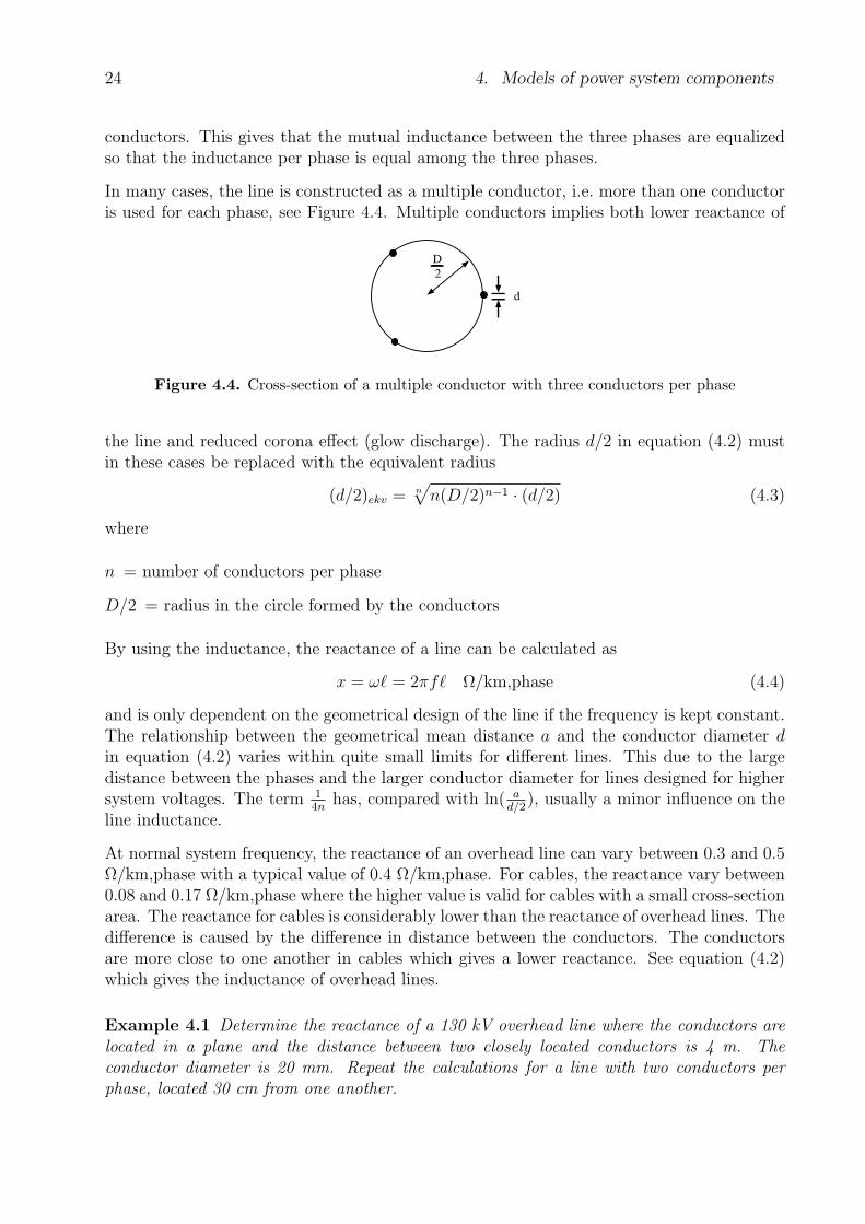
In many cases, the line is constructed as a multiple conductor, i.e. more than one conductoris used for each phase, see Figure 4.4. Multiple conductors implies both lower reactance of
D
2
d
Figure 4.4. Cross-section of a multiple conductor with three conductors per phase
the line and reduced corona effect (glow discharge). The radius d/2 in equation (4.2) mustin these cases be replaced with the equivalent radius
(d/2)ekv = n√
n(D/2)n−1 · (d/2) (4.3)
where
n = number of conductors per phase
D/2 = radius in the circle formed by the conductors
By using the inductance, the reactance of a line can be calculated as
x = ω` = 2πf` Ω/km,phase (4.4)
and is only dependent on the geometrical design of the line if the frequency is kept constant.The relationship between the geometrical mean distance a and the conductor diameter din equation (4.2) varies within quite small limits for different lines. This due to the largedistance between the phases and the larger conductor diameter for lines designed for highersystem voltages. The term 1
4nhas, compared with ln( a
d/2), usually a minor influence on the
line inductance.
At normal system frequency, the reactance of an overhead line can vary between 0.3 and 0.5Ω/km,phase with a typical value of 0.4 Ω/km,phase. For cables, the reactance vary between0.08 and 0.17 Ω/km,phase where the higher value is valid for cables with a small cross-sectionarea. The reactance for cables is considerably lower than the reactance of overhead lines. Thedifference is caused by the difference in distance between the conductors. The conductorsare more close to one another in cables which gives a lower reactance. See equation (4.2)which gives the inductance of overhead lines.
Example 4.1 Determine the reactance of a 130 kV overhead line where the conductors arelocated in a plane and the distance between two closely located conductors is 4 m. Theconductor diameter is 20 mm. Repeat the calculations for a line with two conductors perphase, located 30 cm from one another.
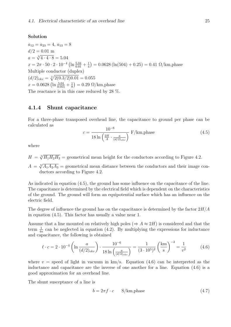
4.1. Electrical characteristic of an overhead line 25
Solution
a12 = a23 = 4, a13 = 8
d/2 = 0.01 m
a = 3√
4 · 4 · 8 = 5.04
x = 2π · 50 · 2 · 10−4(ln 5.04
0.01+ 1
4
)= 0.0628 (ln(504) + 0.25) = 0.41 Ω/km,phase
Multiple conductor (duplex)
(d/2)ekv = 2√
2(0.3/2)0.01 = 0.055
x = 0.0628(ln 5.04
0.055+ 1
8
)= 0.29 Ω/km,phase
The reactance is in this case reduced by 28 %.
4.1.4 Shunt capacitance
For a three-phase transposed overhead line, the capacitance to ground per phase can becalculated as
c =10−6
18 ln(
2HA· a
(d/2)ekv
) F/km,phase (4.5)
where
H = 3√
H1H2H3 = geometrical mean height for the conductors according to Figure 4.2.
A = 3√
A1A2A3 = geometrical mean distance between the conductors and their image con-ductors according to Figure 4.2.
As indicated in equation (4.5), the ground has some influence on the capacitance of the line.The capacitance is determined by the electrical field which is dependent on the characteristicsof the ground. The ground will form an equipotential surface which has an influence on theelectric field.
The degree of influence the ground has on the capacitance is determined by the factor 2H/Ain equation (4.5). This factor has usually a value near 1.
Assume that a line mounted on relatively high poles (⇒ A ≈ 2H) is considered and that theterm 1
4ncan be neglected in equation (4.2). By multiplying the expressions for inductance
and capacitance, the following is obtained
` · c = 2 · 10−4
(ln
a
(d/2)ekv
)· 10−6
18 ln(
a(d/2)ekv
) =1
(3 · 105)2
(km
s
)−2
=1
v2(4.6)
where v = speed of light in vacuum in km/s. Equation (4.6) can be interpreted as theinductance and capacitance are the inverse of one another for a line. Equation (4.6) is agood approximation for an overhead line.
The shunt susceptance of a line is
b = 2πf · c S/km,phase (4.7)

26 4. Models of power system components
A typical value of the shunt susceptance of a line is 3 · 10−6 S/km,phase. Cables haveconsiderable higher values between 3 · 10−5 – 3 · 10−4 S/km,phase.
Example 4.2 Assume that a line has a shunt susceptance of 3 · 10−6 S/km,phase. Useequation (4.6) to estimate the reactance of the line.
Solution
x = ω` ≈ ω
cv2=
ω2
bv2=
(100π)2
3 · 10−6(3 · 105)2= 0.366 Ω/km
which is near the standard value of 0.4 Ω/km for the reactance of an overhead line.
4.2 Model of a line
Both overhead lines and cables have their electrical quantities r, x, g and b distributed alongthe whole length. Figure 4.1 shows an approximation of the distribution of the quantities.Generally, the accuracy of the calculation result will increase with the number of distributedquantities.
At a first glance, it seems possible to form a line model where the total resistance/inductanceis calculated as the product between the resistance/inductance per length unit and the lengthof the line. This approximation is though only valid for short lines and lines of mediumlength. For long lines, the distribution of the quantities r, x, g and b must be taken intoaccount. Such analysis can be carried out with help of differential calculus.
There are no absolute limits between short, medium and long lines. Usually, lines shorterthan 100 km are considered as short, between 100 km and 300 km as medium long and lineslonger than 300 km are classified as long. For cables, having considerable higher values ofthe shunt capacitance, the distance 100 km should be considered as medium long. In thefollowing, models for short and medium long lines are given.
4.2.1 Short lines
In short line models, the shunt parameters are neglected, i.e. conductance and susceptance.This because the current flowing through these components is less than one percent of therated current of the line. The short line model is given in Figure 4.5. This single-phasemodel of a three-phase system is valid under the assumption that the system is operatingunder symmetrical conditions.
The impedance of the line can be calculated as
Z = R + jX = (r + jx)s Ω/phase (4.8)
where s = the length of the line in km.

4.2. Model of a line 27
Uk Uj
IkZ = R + jX
Figure 4.5. Short line model of a line
The relationship between voltage and current in Figure 4.5 is
U j = Uk −√
3(R + jX)Ik (4.9)
where Uk =√
3Uk−phase and U j =√
3U j−phase.
4.2.2 Medium long lines
For lines having a length between 100 and 300 km, the shunt capacitance cannot be neglected.The model shown in Figure 4.5 has to be extended with the shunt susceptance, whichresults in a model called the π-equivalent shown in Figure 4.6. The impedance is calculated
Uk Uj
IkZ = R + jX
Y = jB Y = jB
I
Figure 4.6. Medium long model of a line
according to equation (4.8) and the admittance to ground per phase is obtained as
Y = jB = jbs
2S (4.10)
i.e. the total shunt capacitance of the line is divided into two equal parts, one at each endof the line. The π-equivalent is a very common and useful model in power system analysis.
The electrical behavior of the model is described by
U j = Uk −√
3ZI (4.11)
I = Ik − YUk√
3(4.12)
which results inU j =
(1 + ZY
)Uk −
√3ZIk (4.13)

28 4. Models of power system components
4.3 Single-phase transformer
The principle diagram of a two winding transformer is shown in Figure 4.7. The fundamentalprinciples of a transformer are given in the figure. In a real transformer, the demand ofa strong magnetic coupling between the primary and secondary sides must be taken intoaccount in the design.
Iron core
Primary
winding
N 1 turns
Secondary
winding
N 2 turns
Figure 4.7. Principle design of a two winding transformer
Assume that the magnetic flux can be divided into three components. There is a core flux Φm
passing through both the primary and the secondary windings. There are also leakage fluxes,Φl1 passing only the primary winding and Φl2 which passes only the secondary winding. Theresistance of the primary winding is r1 and for the secondary winding r2. According to thelaw of induction, the following relationships can be given for the voltages at the transformerterminals :
u1 = r1i1 + N1d(Φl1 + Φm)
dt(4.14)
u2 = r2i′2 + N2
d(Φl2 + Φm)
dt
Assuming linear conditions, the following is valid
N1Φl1 = Ll1i1 (4.15)
N2Φl2 = Ll2i′2
where
Ll1 = inductance of the primary winding
Ll2 = inductance of the secondary winding

4.3. Single-phase transformer 29
Equation (4.14) can be rewritten as
u1 = r1i1 + Ll1di1dt
+ N1dΦm
dt(4.16)
u2 = r2i′2 + Ll2
di′2dt
+ N2dΦm
dt
With the reluctance R of the iron core and the definitions of the directions of the currentsaccording to Figure 4.7, the magnetomotive forces N1i1 and N2i
′2 can be added as
N1i1 + N2i′2 = RΦm (4.17)
Assume that i′2 = 0, i.e. the secondary side of the transformer is not connected. The currentnow flowing in the primary winding is called the magnetizing current and the magnitude canbe calculated using equation (4.17) as
im =RΦm
N1
(4.18)
If equation (4.18) is inserted into equation (4.17), the result is
i1 = im − N2
N1
i′2 = im +N2
N1
i2 (4.19)
wherei2 = −i′2 (4.20)
Assuming linear conditions, the induced voltage drop N1dΦmdt
in equation (4.16) can beexpressed by using an inductor as
N1dΦm
dt= Lm
dimdt
(4.21)
i.e. Lm = N21 /R. By using equations (4.16), (4.19) and (4.21), the equivalent diagram of a
single-phase transformer can be drawn, see Figure 4.8.
Figure 4.8. Equivalent diagram of a single-phase transformer
In Figure 4.8, one part of the ideal transformer is shown, which is a lossless transformerwithout leakage fluxes and magnetizing currents.
30 4. Models of power system components
The equivalent diagram in Figure 4.8 has the advantage that the different parts representsdifferent parts of the real transformer. For example, the inductance Lm represents theassumed linear relationship between the core flux Φm and the magnetomotive force of theiron core. Also the resistive copper losses in the transformer are represented by r1 and r2.
In power system analysis, where the transformer is modeled, a simplified model is often usedwhere the magnetizing current is neglected.
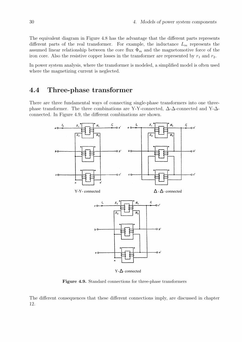
4.4 Three-phase transformer
There are three fundamental ways of connecting single-phase transformers into one three-phase transformer. The three combinations are Y-Y-connected, ∆-∆-connected and Y-∆-connected. In Figure 4.9, the different combinations are shown.
Y-Y- connected ∆ - connected∆-
Y-∆- connected
Figure 4.9. Standard connections for three-phase transformers
The different consequences that these different connections imply, are discussed in chapter12.
Chapter 5
Important theorems in power system analysis
In many cases, the use of theorems can simplify the analysis of electrical circuits and systems.In the following sections, some important theorems will be discussed and proofs will be given.
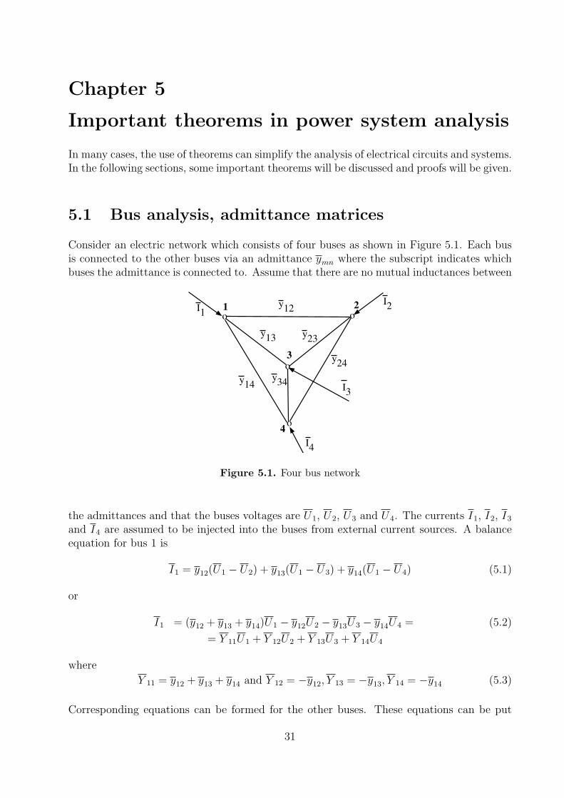
5.1 Bus analysis, admittance matrices
Consider an electric network which consists of four buses as shown in Figure 5.1. Each busis connected to the other buses via an admittance ymn where the subscript indicates whichbuses the admittance is connected to. Assume that there are no mutual inductances between
o o
o
o
y12
y23
y13
y14
y24
y34
1
3
4
2I2I
1
I4
I3
Figure 5.1. Four bus network
the admittances and that the buses voltages are U1, U2, U3 and U4. The currents I1, I2, I3
and I4 are assumed to be injected into the buses from external current sources. A balanceequation for bus 1 is
I1 = y12(U1 − U2) + y13(U1 − U3) + y14(U1 − U4) (5.1)
or
I1 = (y12 + y13 + y14)U1 − y12U2 − y13U3 − y14U4 = (5.2)
= Y 11U1 + Y 12U2 + Y 13U3 + Y 14U4
where
Y 11 = y12 + y13 + y14 and Y 12 = −y12, Y 13 = −y13, Y 14 = −y14 (5.3)
Corresponding equations can be formed for the other buses. These equations can be put
31
32 5. Important theorems in power system analysis
together to a matrix equation as :
I =
I1
I2
I3
I4
=
Y 11Y 12Y 13Y 14
Y 21Y 22Y 23Y 24
Y 31Y 32Y 33Y 34
Y 41Y 42Y 43Y 44
U1
U2
U3
U4
= YU (5.4)
This matrix is called the bus admittance matrix or Y-bus matrix. The following propertiesare valid :
• It can be uniquely determined from a given admittance network.
• The diagonal element Y kk = the sum of all admittances connected to bus k.
• Non-diagonal element Y ik = −yik where yik is the admittance between bus i and busk.
• This gives that the matrix is symmetric, i.e. Y ik = Y ki (one exception is when thenetwork includes phase shifting transformers).
• It is singular since I1 + I2 + I3 + I4 = 0
If the potential in one bus is assumed to be = 0, the corresponding line and column in theadmittance matrix can be taken away which results in a non-singular matrix. Bus analysisusing the Y-bus matrix is the method most often used when studying larger, meshed networksin a systematic manner.
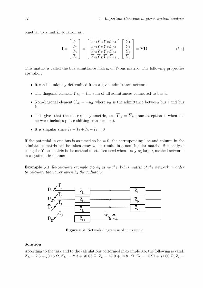
Example 5.1 Re-calculate example 3.5 by using the Y-bus matrix of the network in orderto calculate the power given by the radiators.
o
o
o
o
o
o
o
o
ZL
ZL
ZL
ZL0
Za
Zb
Zc
I2
I3
I0
I1
I4
U1
U2
U3
U0
U4
Figure 5.2. Network diagram used in example
Solution
According to the task and to the calculations performed in example 3.5, the following is valid;ZL = 2.3 + j0.16 Ω, ZL0 = 2.3 + j0.03 Ω, Za = 47.9 + j4.81 Ω, Zb = 15.97 + j1.60 Ω, Zc =
5.1. Bus analysis, admittance matrices 33
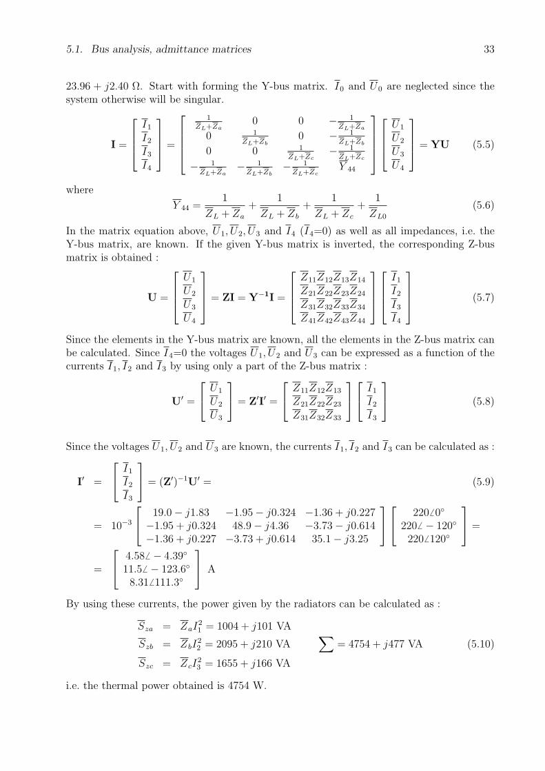
23.96 + j2.40 Ω. Start with forming the Y-bus matrix. I0 and U0 are neglected since thesystem otherwise will be singular.
I =
I1
I2
I3
I4
=
1ZL+Za
0 0 − 1ZL+Za
0 1ZL+Zb
0 − 1ZL+Zb
0 0 1ZL+Zc
− 1ZL+Zc
− 1ZL+Za
− 1ZL+Zb
− 1ZL+Zc
Y 44
U1
U2
U3
U4
= YU (5.5)
where
Y 44 =1
ZL + Za
+1
ZL + Zb
+1
ZL + Zc
+1
ZL0
(5.6)
In the matrix equation above, U1, U2, U3 and I4 (I4=0) as well as all impedances, i.e. theY-bus matrix, are known. If the given Y-bus matrix is inverted, the corresponding Z-busmatrix is obtained :
U =
U1
U2
U3
U4
= ZI = Y−1I =
Z11Z12Z13Z14
Z21Z22Z23Z24
Z31Z32Z33Z34
Z41Z42Z43Z44
I1
I2
I3
I4
(5.7)
Since the elements in the Y-bus matrix are known, all the elements in the Z-bus matrix canbe calculated. Since I4=0 the voltages U1, U2 and U3 can be expressed as a function of thecurrents I1, I2 and I3 by using only a part of the Z-bus matrix :
U′ =
U1
U2
U3
= Z′I′ =
Z11Z12Z13
Z21Z22Z23
Z31Z32Z33
I1
I2
I3
(5.8)
Since the voltages U1, U2 and U3 are known, the currents I1, I2 and I3 can be calculated as :
I′ =
I1
I2
I3
= (Z′)−1U′ = (5.9)
= 10−3
19.0− j1.83 −1.95− j0.324 −1.36 + j0.227−1.95 + j0.324 48.9− j4.36 −3.73− j0.614−1.36 + j0.227 −3.73 + j0.614 35.1− j3.25
220 6 0
2206 − 120
220 6 120
=
=
4.586 − 4.39
11.56 − 123.6
8.31 6 111.3
A
By using these currents, the power given by the radiators can be calculated as :
Sza = ZaI21 = 1004 + j101 VA
Szb = ZbI22 = 2095 + j210 VA
∑= 4754 + j477 VA (5.10)
Szc = ZcI23 = 1655 + j166 VA
i.e. the thermal power obtained is 4754 W.

34 5. Important theorems in power system analysis
5.2 Millman’s theorem
Millman’s theorem (the parallel generator-theorem) gives that if a number of admittancesY 1, Y 2, Y 3 . . . Y n are connected to a common bus k, and the voltages to a reference busU10, U20, U30 . . . Un0 are known, the voltage between bus k and the reference bus, Uk0 canbe calculated as
Uk0 =
n∑i=1
Y iU i0
n∑i=1
Y i
(5.11)
Assume a Y-connection of admittances as shown in Figure 5.3. The Y-bus matrix for this
Figure 5.3. Y-connected admittances
network can be formed as
I1
I2...
In
Ik
=
Y 1 0 . . . 0 −Y 1
0 Y 2 . . . 0 −Y 2...
.... . .
......
0 0 . . . Y n −Y n
−Y 1 −Y 2 . . . −Y n (Y 1 + Y 2 + . . . Y n)
U10
U20...
Un0
Uk0
(5.12)
This equation can be written as
I1
I2...
Ik
=
(U10Y 1 − Uk0Y 1)(U20Y 2 − Uk0Y 2
...(−U10Y 1 − U20Y 2 − . . . +
∑ni=1 Y iUk0
(5.13)
Since no current is injected at bus k (Ik = 0), the last equation can be written as
Ik = 0 = −U10Y 1 − U20Y 2 − . . . +n∑
i=1
Y iUk0 (5.14)
5.2. Millman’s theorem 35
This equation can be written as
Uk0 =U10Y 1 + U20Y 2 + . . . + Un0Y n
n∑i=1
Y i
(5.15)
and by that, the proof of the Millman’s theorem is completed.
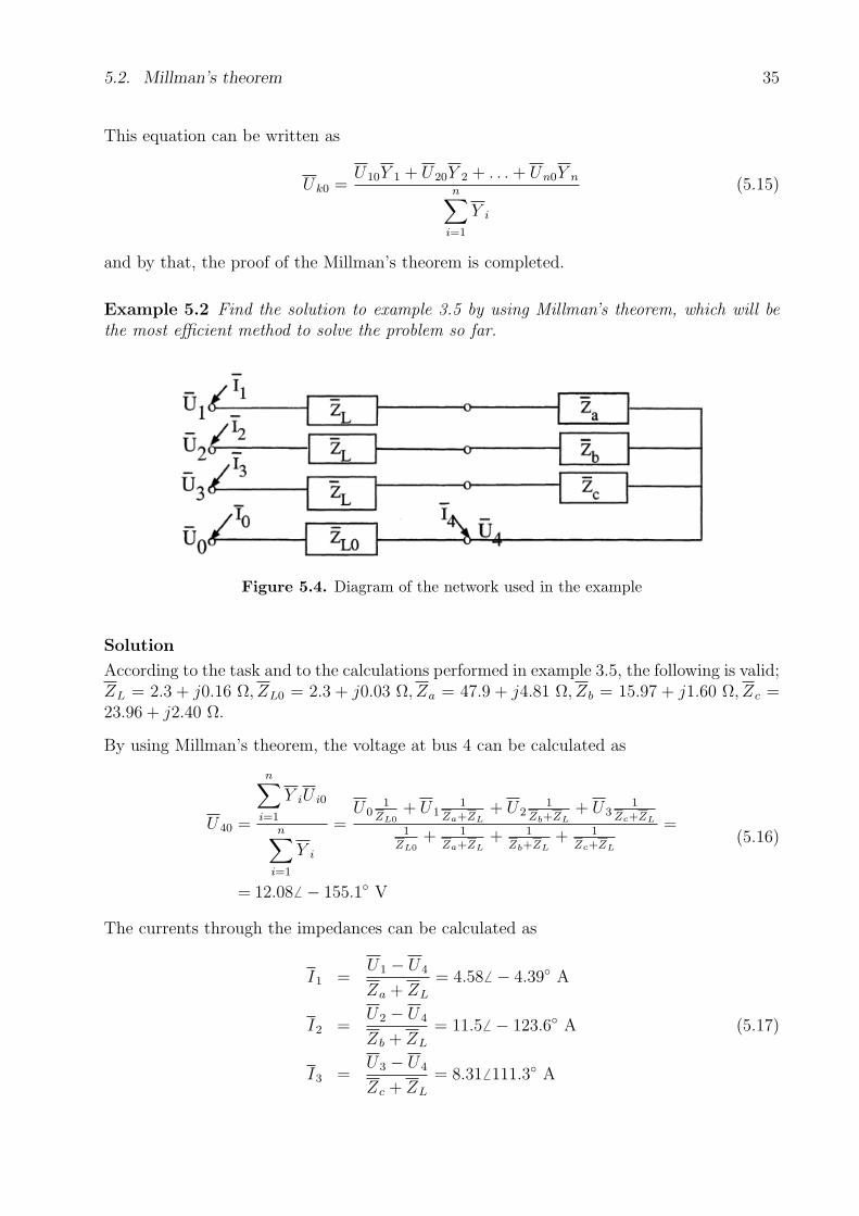
Example 5.2 Find the solution to example 3.5 by using Millman’s theorem, which will bethe most efficient method to solve the problem so far.
Figure 5.4. Diagram of the network used in the example
Solution
According to the task and to the calculations performed in example 3.5, the following is valid;ZL = 2.3 + j0.16 Ω, ZL0 = 2.3 + j0.03 Ω, Za = 47.9 + j4.81 Ω, Zb = 15.97 + j1.60 Ω, Zc =23.96 + j2.40 Ω.
By using Millman’s theorem, the voltage at bus 4 can be calculated as
U40 =
n∑i=1
Y iU i0
n∑i=1
Y i
=U0
1ZL0
+ U11
Za+ZL+ U2
1Zb+ZL
+ U31
Zc+ZL
1ZL0
+ 1Za+ZL
+ 1Zb+ZL
+ 1Zc+ZL
=
= 12.086 − 155.1 V
(5.16)
The currents through the impedances can be calculated as
I1 =U1 − U4
Za + ZL
= 4.586 − 4.39 A
I2 =U2 − U4
Zb + ZL
= 11.5 6 − 123.6 A (5.17)
I3 =U3 − U4
Zc + ZL
= 8.316 111.3 A
36 5. Important theorems in power system analysis
By using these currents, the power from the radiators can be calculated in the same way asearlier :
Sza = ZaI21 = 1004 + j101 VA
Szb = ZbI22 = 2095 + j210 VA
∑= 4754 + j477 VA (5.18)
Szc = ZcI23 = 1655 + j166 VA
i.e. the thermal power is 4754 W.
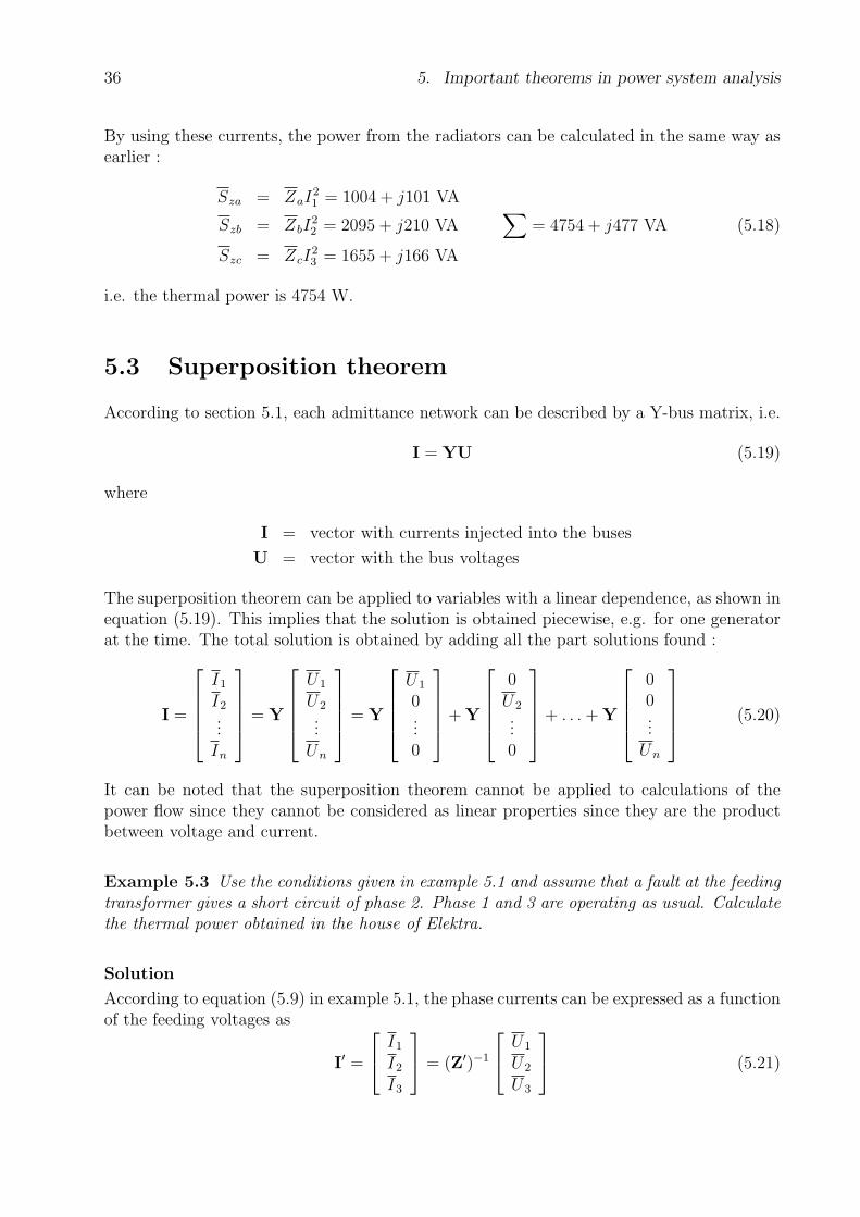
5.3 Superposition theorem
According to section 5.1, each admittance network can be described by a Y-bus matrix, i.e.
I = YU (5.19)
where
I = vector with currents injected into the buses
U = vector with the bus voltages
The superposition theorem can be applied to variables with a linear dependence, as shown inequation (5.19). This implies that the solution is obtained piecewise, e.g. for one generatorat the time. The total solution is obtained by adding all the part solutions found :
I =
I1
I2...
In
= Y
U1
U2...
Un
= Y
U1
0...0
+ Y
0U2...0
+ . . . + Y
00...
Un
(5.20)
It can be noted that the superposition theorem cannot be applied to calculations of thepower flow since they cannot be considered as linear properties since they are the productbetween voltage and current.
Example 5.3 Use the conditions given in example 5.1 and assume that a fault at the feedingtransformer gives a short circuit of phase 2. Phase 1 and 3 are operating as usual. Calculatethe thermal power obtained in the house of Elektra.
Solution
According to equation (5.9) in example 5.1, the phase currents can be expressed as a functionof the feeding voltages as
I′ =
I1
I2
I3
= (Z′)−1
U1
U2
U3
(5.21)
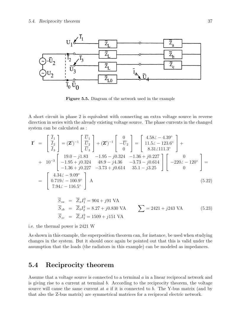
5.4. Reciprocity theorem 37
Figure 5.5. Diagram of the network used in the example
A short circuit in phase 2 is equivalent with connecting an extra voltage source in reversedirection in series with the already existing voltage source. The phase currents in the changedsystem can be calculated as :
I′ =
I1
I2
I3
= (Z′)−1
U1
U2
U3
+ (Z′)−1
0−U2
0
=
4.586 − 4.39
11.5 6 − 123.6
8.316 111.3
+
+ 10−3
19.0− j1.83 −1.95− j0.324 −1.36 + j0.227−1.95 + j0.324 48.9− j4.36 −3.73− j0.614−1.36 + j0.227 −3.73 + j0.614 35.1− j3.25
0−2206 − 120
0
=
=
4.34 6 − 9.09
0.719 6 − 100.9
7.946 − 116.5
A (5.22)
Sza = ZaI21 = 904 + j91 VA
Szb = ZbI22 = 8.27 + j0.830 VA
∑= 2421 + j243 VA (5.23)
Szc = ZcI23 = 1509 + j151 VA
i.e. the thermal power is 2421 W
As shown in this example, the superposition theorem can, for instance, be used when studyingchanges in the system. But it should once again be pointed out that this is valid under theassumption that the loads (the radiators in this example) can be modeled as impedances.
5.4 Reciprocity theorem
Assume that a voltage source is connected to a terminal a in a linear reciprocal network andis giving rise to a current at terminal b. According to the reciprocity theorem, the voltagesource will cause the same current at a if it is connected to b. The Y-bus matrix (and bythat also the Z-bus matrix) are symmetrical matrices for a reciprocal electric network.
38 5. Important theorems in power system analysis
Assume that an electric network with n buses can be described by a symmetric Y-bus matrix,i.e.
I1
I2...
In
= I = YU =
Y 11 Y 12 . . . Y 1n
Y 21 Y 22 . . . Y 2n...
.... . .
...Y n1 Y n2 . . . Y nn
U1
U2...
Un
(5.24)
Assume that all voltages are = 0 except Ua. The current at b can now be calculated as
Ib = Y baUa (5.25)
Assume instead that all voltages are = 0 except U b. This means that the current at a is
Ia = Y abU b (5.26)
If Ua = U b, the currents Ia and Ib will be equal since the Y-bus matrix is symmetric, i.e.Y ab = Y ba. By that, the proof of the reciprocity theorem is completed.
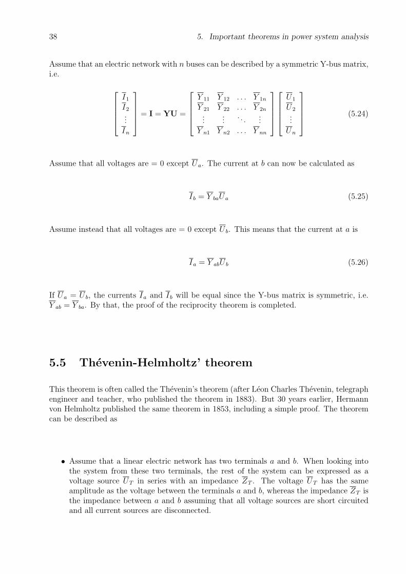
5.5 Thevenin-Helmholtz’ theorem
This theorem is often called the Thevenin’s theorem (after Leon Charles Thevenin, telegraphengineer and teacher, who published the theorem in 1883). But 30 years earlier, Hermannvon Helmholtz published the same theorem in 1853, including a simple proof. The theoremcan be described as
• Assume that a linear electric network has two terminals a and b. When looking intothe system from these two terminals, the rest of the system can be expressed as avoltage source UT in series with an impedance ZT . The voltage UT has the sameamplitude as the voltage between the terminals a and b, whereas the impedance ZT isthe impedance between a and b assuming that all voltage sources are short circuitedand all current sources are disconnected.

5.5. Thevenin-Helmholtz’ theorem 39
Proof :Assume that a linear network has twoterminals, a and b, where the voltagebetween the terminals equals UT . Be-tween a and b an impedance Z is con-nected giving a current I through theimpedance. This is equal with hav-ing a network with a voltage sourceUT between a and b in series with theimpedance Z, together with having anetwork with the voltage source −UT
and the other voltage sources in thenetwork shortened. By using the su-perposition theorem, the current I canbe calculated as the sum of I1 and I2.The current I1 = 0 since the voltage isequal on both sides of the impedanceZ. The current I2 = 0 can be calcu-lated as I2 = −(−UT )/(Z + ZT ) sincethe network impedance between a andb is ZT . The conclusion is that
a
b
I
Z
=
linear
electric
network
I1
~ UT
a
b
electric
linear
network
+
~ UT
I2 Za
b
voltage
sources
Z
shortened
I = I1 + I2 =UT
Z + ZT
(5.27)
which is the same as obtained by the Thevenin-Helmholtz’ theorem, viz.
a
b
~ UT =
b
a
ZTU
T~
linear
electric
network

40 5. Important theorems in power system analysis

Chapter 6
Analysis of symmetric three-phase systems
The analysis of a three-phase system operating in symmetric conditions can be carried outby studying only one phase. In Figure 6.1, a simple three-phase system is shown. Since the
Ia
+
Ua
ZG
ZL
ZL
Ib
Ic
In=0
~
~
~ ZL
Zn
ZG
ZG
Uc
Ub
nN
+
+
Figure 6.1. Symmetric three-phase system
system is operating in symmetric conditions, the neutral connection points at the generatorand at the load have both the same potential which means that In = 0. The impedance inthe neutral conductor Zn is therefore of no importance. The equations for phase a can beformulated as :
Ua = (ZG + ZL)Ia (6.1)
The currents and voltages in the other phases have all the same amplitude as in phase abut they have a phase displacement of 120. Equation (6.1) corresponds to the single-phasemodeling of the network in Figure 6.2. The solution to this system gives also the completesolution to the whole system in Figure 6.1.
Ia
+Z=R+jX
~Ua
ZGZL
Figure 6.2. Single-phase equivalent of a symmetric three-phase system
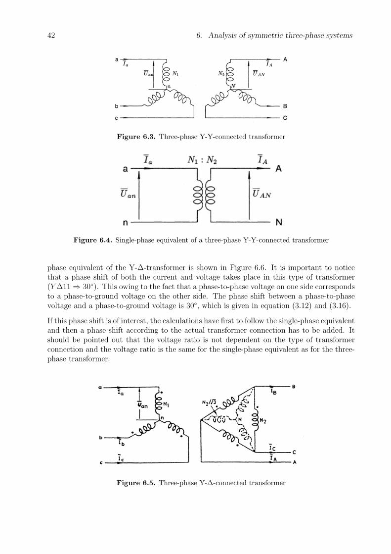
Assume that one part of a network consists of a Y-Y-connected three-phase transformer, seeFigure 6.3. The single-phase equivalent is given in Figure 6.4 having the same turns-ratio asthe three-phase transformer.
If the transformer is Y-∆-connected according to Figure 6.5, the ∆-side must be replacedby an equivalent Y-connection as indicated with dashed windings in the figure. The single-
41
42 6. Analysis of symmetric three-phase systems
Figure 6.3. Three-phase Y-Y-connected transformer
Figure 6.4. Single-phase equivalent of a three-phase Y-Y-connected transformer
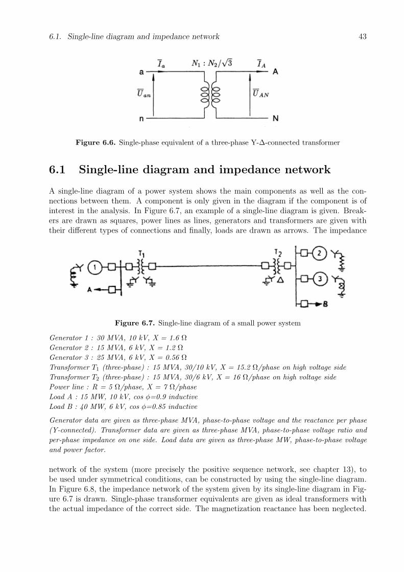
phase equivalent of the Y-∆-transformer is shown in Figure 6.6. It is important to noticethat a phase shift of both the current and voltage takes place in this type of transformer(Y ∆11 ⇒ 30). This owing to the fact that a phase-to-phase voltage on one side correspondsto a phase-to-ground voltage on the other side. The phase shift between a phase-to-phasevoltage and a phase-to-ground voltage is 30, which is given in equation (3.12) and (3.16).
If this phase shift is of interest, the calculations have first to follow the single-phase equivalentand then a phase shift according to the actual transformer connection has to be added. Itshould be pointed out that the voltage ratio is not dependent on the type of transformerconnection and the voltage ratio is the same for the single-phase equivalent as for the three-phase transformer.
Figure 6.5. Three-phase Y-∆-connected transformer
6.1. Single-line diagram and impedance network 43
Figure 6.6. Single-phase equivalent of a three-phase Y-∆-connected transformer
6.1 Single-line diagram and impedance network
A single-line diagram of a power system shows the main components as well as the con-nections between them. A component is only given in the diagram if the component is ofinterest in the analysis. In Figure 6.7, an example of a single-line diagram is given. Break-ers are drawn as squares, power lines as lines, generators and transformers are given withtheir different types of connections and finally, loads are drawn as arrows. The impedance
Figure 6.7. Single-line diagram of a small power system
Generator 1 : 30 MVA, 10 kV, X = 1.6 ΩGenerator 2 : 15 MVA, 6 kV, X = 1.2 ΩGenerator 3 : 25 MVA, 6 kV, X = 0.56 ΩTransformer T1 (three-phase) : 15 MVA, 30/10 kV, X = 15.2 Ω/phase on high voltage sideTransformer T2 (three-phase) : 15 MVA, 30/6 kV, X = 16 Ω/phase on high voltage sidePower line : R = 5 Ω/phase, X = 7 Ω/phaseLoad A : 15 MW, 10 kV, cos φ=0.9 inductiveLoad B : 40 MW, 6 kV, cos φ=0.85 inductive
Generator data are given as three-phase MVA, phase-to-phase voltage and the reactance per phase(Y-connected). Transformer data are given as three-phase MVA, phase-to-phase voltage ratio andper-phase impedance on one side. Load data are given as three-phase MW, phase-to-phase voltageand power factor.
network of the system (more precisely the positive sequence network, see chapter 13), tobe used under symmetrical conditions, can be constructed by using the single-line diagram.In Figure 6.8, the impedance network of the system given by its single-line diagram in Fig-ure 6.7 is drawn. Single-phase transformer equivalents are given as ideal transformers withthe actual impedance of the correct side. The magnetization reactance has been neglected.

44 6. Analysis of symmetric three-phase systems
Gen 1 Load A Transf. T1 Line Transf. T2 Load B Gen 2 Gen 3
Figure 6.8. Impedance network of a small power system
Generators are represented as a voltage source behind an impedance. Power lines are givenas Π-equivalents and the loads are represented as impedances. The different connections oftransformers and earthing impedances are not represented as symmetrical conditions apply.
The system has three different voltage levels (6, 10 and 30 kV). The analysis of the systemcan be carried out due to a transformation of the different voltage levels and impedances toone specific voltage level, e.g. the voltage of the power line, 30 kV. This method gives oftenquite extensive calculations. The normal procedure when analyzing a system with differentvoltage levels is to take advantage of the per-unit system.
6.2 Per-unit (pu) system
A common method to express voltages, currents, powers and impedances in an electricnetwork is in per-unit (or percent) of a certain base or reference value. The per-unit valueof a certain quantity is defined as
Per-unit value =true value
base value of the quantity(6.2)
The per-unit method is very suitable for power systems with several voltage levels andtransformers. In a three-phase system, the per-unit value can be calculated using the corre-sponding base quantity. By using the base voltage
Ub = phase-to-phase voltage = base voltage, kV (6.3)
and a base power,Sb = three-phase base power, MVA (6.4)
the base current
Ib =Sb√3Ub
= base current/phase, kA (6.5)
as well as a base impedance
Zb =U2
b
Sb
= base impedance, Ω (6.6)
6.2. Per-unit (pu) system 45
can be calculated. In expressions given above, the units kV and MVA have been assumed,which implies units in kA and Ω. Of course, different combinations of units can be used, e.g.V, VA, A, Ω or kV, kVA, A, kΩ.
The reasons why using the per-unit system are (among other things)
• The percentage voltage drop is directly given in the per-unit voltage.
• It is possible to analyze power systems having different voltage levels in a more efficientway.
• When having different voltage levels, the relative importance of different impedancesis directly given by the per-unit value.
• When having large systems, numerical values of the same magnitude are obtainedwhich increase the numerical accuracy of the analysis.
6.2.1 Per-unit representation of transformers
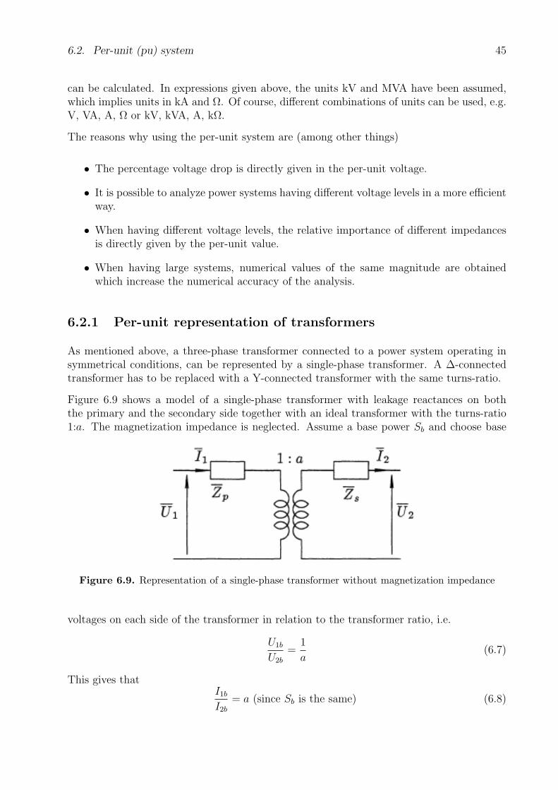
As mentioned above, a three-phase transformer connected to a power system operating insymmetrical conditions, can be represented by a single-phase transformer. A ∆-connectedtransformer has to be replaced with a Y-connected transformer with the same turns-ratio.
Figure 6.9 shows a model of a single-phase transformer with leakage reactances on boththe primary and the secondary side together with an ideal transformer with the turns-ratio1:a. The magnetization impedance is neglected. Assume a base power Sb and choose base
Figure 6.9. Representation of a single-phase transformer without magnetization impedance
voltages on each side of the transformer in relation to the transformer ratio, i.e.
U1b
U2b
=1
a(6.7)
This gives thatI1b
I2b
= a (since Sb is the same) (6.8)
46 6. Analysis of symmetric three-phase systems
and
Z1b =U1b√3I1b
, Z2b =U2b√3I2b
(6.9)
By using Figure 6.9, the voltage U2 can be expressed as
U2 = [U1 −√
3I1Zp]a−√
3I2Zs (6.10)
By using the definition (6.2), the equation (6.10) can be rewritten as
U2(pu)U2b = [U1(pu)U1b −√
3I1(pu)I1bZp(pu)Z1b]a− (6.11)√3I2(pu)I2bZs(pu)Z2b
By dividing with U2b and by using the expressions 6.7, 6.8 and 6.9, the following is obtained
U2(pu) = U1(pu)− I1(pu)Zp(pu)− I2(pu)Zs(pu) (6.12)
But sinceI1
I2
=I1b
I2b
= a orI1
I1b
=I2
I2b
(6.13)
the following is validI1(pu) = I2(pu) = I(pu) (6.14)
The equation (6.12) can thereby be rewritten as
U2(pu) = U1(pu)− I(pu)Z(pu) (6.15)
whereZ(pu) = Zp(pu) + Zs(pu) (6.16)
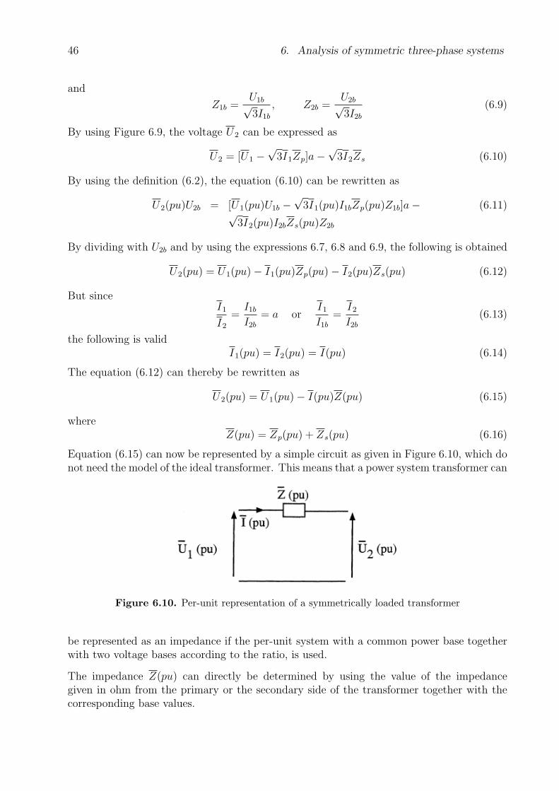
Equation (6.15) can now be represented by a simple circuit as given in Figure 6.10, which donot need the model of the ideal transformer. This means that a power system transformer can
Figure 6.10. Per-unit representation of a symmetrically loaded transformer
be represented as an impedance if the per-unit system with a common power base togetherwith two voltage bases according to the ratio, is used.
The impedance Z(pu) can directly be determined by using the value of the impedancegiven in ohm from the primary or the secondary side of the transformer together with thecorresponding base values.
6.2. Per-unit (pu) system 47
On the primary side :
Z1 = Zp + Zs/a2 (6.17)
Z1(pu) =Z1
Z1b
=Zp
Z1b
+Zs
Z1b
· 1
a2
Buta2Z1b = Z2b (6.18)
which gives thatZ1(pu) = Zp(pu) + Zs(pu) = Z(pu) (6.19)
Of course, the same calculations can be performed using the secondary side of the transformerwith corresponding result. The conclusions is that the per-unit value of the impedance ofthe transformer is independent on the side used in the calculations. It must be pointed outthat if the transformer impedance is given in percent, i.e. internal per-unit, the impedancemust first be converted to system per-unit if another base power and/or bas voltage is used.
Example 6.1 Assume that a 15 MVA transformer has a voltage ratio of 6 kV/30 kV anda short circuit reactance of 8 %. Calculate the pu-impedance when the base power of thesystem is 20 MVA and the base voltage on the 30 kV-side is 33 kV.
Solution
The first value to calculate is the transformer impedance in ohm on the 30 kV-side and afterthat, the per-unit value.
Z30kv =Z%
100Ztrafo−bas =
Z%
100
U2trafo−30kV
Strafo
=j8 · 302
100 · 15= j4.8 Ω
Zpu =Z30kV
Zb−30kV
=Z30kV · Sb
U2b−30kV
=j4.8 · 20
332= j0.088 pu
It is possible to calculate the pu value directly by transforming to a new base value as
Zpu−ny = ZpuSb−ny
Sb
· U2b
U2b−ny
=j8
100
20
15
302
332= j0.088 pu (6.20)
6.2.2 Calculations by using the per-unit system
As shown earlier, based on a single-line diagram, an impedance network can be drawn. Thisnetwork contains transformers which can be replaced by impedances by using the per-unitsystem. The algorithm to follow when analyzing a power system is as follows :
1. Choose a suitable base power for the system. It should be in the same range as therated power of the installed system equipments.
2. Choose a base voltage at one section of the system. The system is divided into differentsections by the transformers.
48 6. Analysis of symmetric three-phase systems
3. Calculate the base voltages in all sections of the system by using the transformer ratios.
4. Calculate all per-unit values of all system components that are connected.
5. Draw a single-line diagram of the system.
6. Perform the analysis asked for.
7. Transform the result back to nominal values.
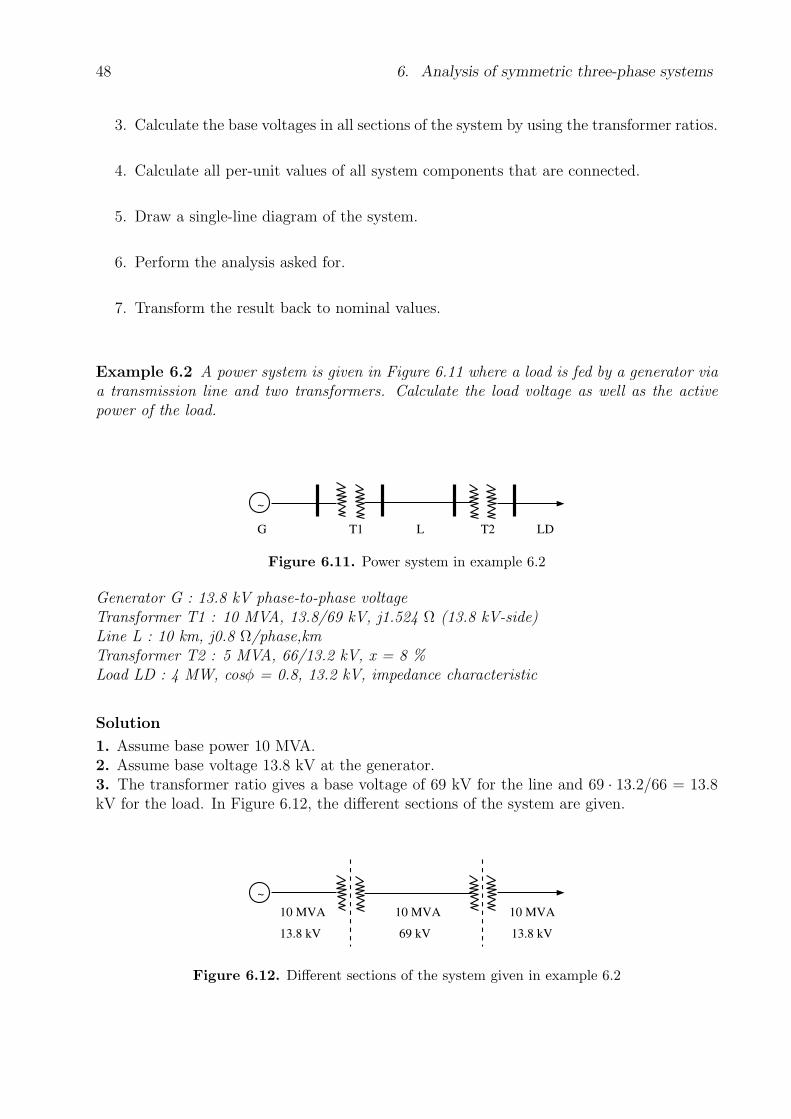
Example 6.2 A power system is given in Figure 6.11 where a load is fed by a generator viaa transmission line and two transformers. Calculate the load voltage as well as the activepower of the load.
~
G T1 L T2 LD
Figure 6.11. Power system in example 6.2
Generator G : 13.8 kV phase-to-phase voltageTransformer T1 : 10 MVA, 13.8/69 kV, j1.524 Ω (13.8 kV-side)Line L : 10 km, j0.8 Ω/phase,kmTransformer T2 : 5 MVA, 66/13.2 kV, x = 8 %Load LD : 4 MW, cosφ = 0.8, 13.2 kV, impedance characteristic
Solution
1. Assume base power 10 MVA.2. Assume base voltage 13.8 kV at the generator.3. The transformer ratio gives a base voltage of 69 kV for the line and 69 · 13.2/66 = 13.8kV for the load. In Figure 6.12, the different sections of the system are given.
10 MVA 10 MVA 10 MVA
13.8 kV 69 kV 13.8 kV
~
Figure 6.12. Different sections of the system given in example 6.2

6.2. Per-unit (pu) system 49
4. Calculate the per-unit values of the system components.
G: Ug =Ug−nom
U1−bas
=13.8
13.8= 1.0 pu
T1: Zt1 =Zt−nom
Z1−bas
= j1.52410
13.82= j0.080 pu
L: ZL =szL
Z2−bas
=10 · j0.8 · 10
692= j0.017 pu
T2: ZT2−13.2kV (Ω) = j8
100
13.22
5= j2.788 Ω
ZT2 =ZT2−13.2kV (Ω)
Z3−bas
=j2.788 · 10
13.82= 0.146 pu
LD: ZLD(Ω) =U2
LD
S∗LD
=U2
LD
SLD(cos φ− j sin φ)=
U2LD
SLD
(cos φ + j sin φ) =
=13.22
4/0.8(0.8 + j0.6) = 27.88 + j20.91 Ω
ZLD =ZLD(Ω)
Z3−bas
=(27.88 + j20.91) · 10
13.82= 1.464 + j1.098 pu
5. By using these values, an impedance network can be drawn as given in Figure 6.13.
Figure 6.13. Impedance network in per-unit
6. The current through the network can be calculated as
I =1 + j0
j0.08 + j0.017 + j0.146 + 1.464 + j1.098= 0.3714− j0.3402 pu (6.21)
The load voltage isULD = IZLD = 0.9173− j0.0903 pu (6.22)
The load power isSLD = ULDI
∗LD = 0.3714 + 0.2785 pu (6.23)
7. The nominal values of the load voltage and active load power can be obtained by multi-plying with corresponding base quantities.
ULDkV = ULDU3−bas =√
0.91732 + 0.0903213.8 = 12.72 kV (6.24)
PLDMW = Real(SLD)Sbas = 0.371 · 10 = 3.71 MW (6.25)

50 6. Analysis of symmetric three-phase systems
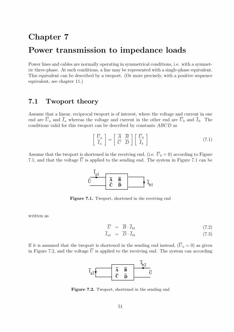
Chapter 7
Power transmission to impedance loads
Power lines and cables are normally operating in symmetrical conditions, i.e. with a symmet-ric three-phase. At such conditions, a line may be represented with a single-phase equivalent.This equivalent can be described by a twoport. (Or more precisely, with a positive sequenceequivalent, see chapter 11.)
7.1 Twoport theory
Assume that a linear, reciprocal twoport is of interest, where the voltage and current in oneend are Ua and Ia whereas the voltage and current in the other end are U b and Ib. Theconditions valid for this twoport can be described by constants ABCD as
[Ua
Ia
]=
[A BC D
] [U b
Ib
](7.1)
Assume that the twoport is shortened in the receiving end, (i.e. U b = 0) according to Figure7.1, and that the voltage U is applied to the sending end. The system in Figure 7.1 can be
Ia1
Ib1
A B
DCU
Figure 7.1. Twoport, shortened in the receiving end
written as
U = B · Ib1 (7.2)
Ia1 = D · Ib1 (7.3)
If it is assumed that the twoport is shortened in the sending end instead, (Ua = 0) as givenin Figure 7.2, and the voltage U is applied to the receiving end. The system can according
C D
BAIa2
Ib2
U
Figure 7.2. Twoport, shortened in the sending end
51
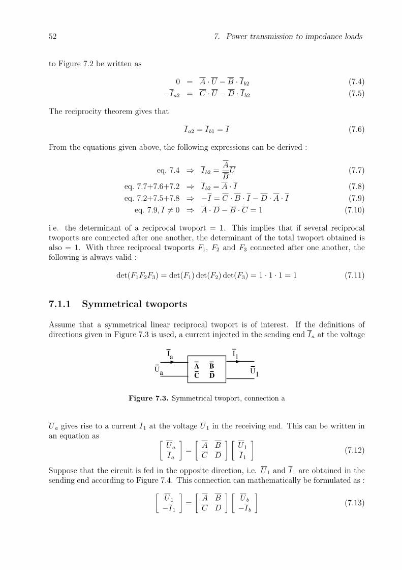
52 7. Power transmission to impedance loads
to Figure 7.2 be written as
0 = A · U −B · Ib2 (7.4)
−Ia2 = C · U −D · Ib2 (7.5)
The reciprocity theorem gives that
Ia2 = Ib1 = I (7.6)
From the equations given above, the following expressions can be derived :
eq. 7.4 ⇒ Ib2 =A
BU (7.7)
eq. 7.7+7.6+7.2 ⇒ Ib2 = A · I (7.8)
eq. 7.2+7.5+7.8 ⇒ −I = C ·B · I −D · A · I (7.9)
eq. 7.9, I 6= 0 ⇒ A ·D −B · C = 1 (7.10)
i.e. the determinant of a reciprocal twoport = 1. This implies that if several reciprocaltwoports are connected after one another, the determinant of the total twoport obtained isalso = 1. With three reciprocal twoports F1, F2 and F3 connected after one another, thefollowing is always valid :
det(F1F2F3) = det(F1) det(F2) det(F3) = 1 · 1 · 1 = 1 (7.11)
7.1.1 Symmetrical twoports
Assume that a symmetrical linear reciprocal twoport is of interest. If the definitions ofdirections given in Figure 7.3 is used, a current injected in the sending end Ia at the voltage
Ia
I1
A B
DCU
a U1
Figure 7.3. Symmetrical twoport, connection a
Ua gives rise to a current I1 at the voltage U1 in the receiving end. This can be written inan equation as [
Ua
Ia
]=
[A BC D
] [U1
I1
](7.12)
Suppose that the circuit is fed in the opposite direction, i.e. U1 and I1 are obtained in thesending end according to Figure 7.4. This connection can mathematically be formulated as :
[U1
−I1
]=
[A BC D
] [U b
−Ib
](7.13)
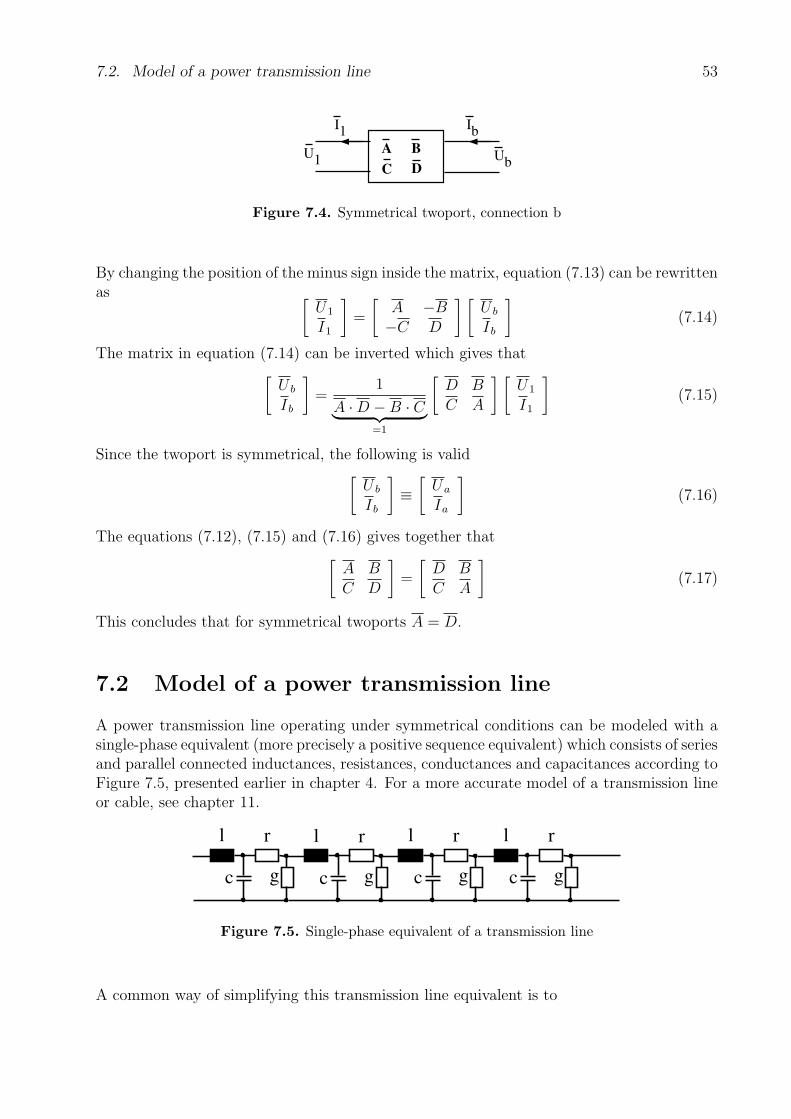
7.2. Model of a power transmission line 53
C D
BA
I1
Ib
U1 U
b
Figure 7.4. Symmetrical twoport, connection b
By changing the position of the minus sign inside the matrix, equation (7.13) can be rewrittenas [
U1
I1
]=
[A −B−C D
] [U b
Ib
](7.14)
The matrix in equation (7.14) can be inverted which gives that[
U b
Ib
]=
1
A ·D −B · C︸ ︷︷ ︸=1
[D BC A
] [U1
I1
](7.15)
Since the twoport is symmetrical, the following is valid[
U b
Ib
]≡
[Ua
Ia
](7.16)
The equations (7.12), (7.15) and (7.16) gives together that[
A BC D
]=
[D BC A
](7.17)
This concludes that for symmetrical twoports A = D.
7.2 Model of a power transmission line
A power transmission line operating under symmetrical conditions can be modeled with asingle-phase equivalent (more precisely a positive sequence equivalent) which consists of seriesand parallel connected inductances, resistances, conductances and capacitances according toFigure 7.5, presented earlier in chapter 4. For a more accurate model of a transmission lineor cable, see chapter 11.
l r
c g
l r
c g
l r
c g
l r
c g
Figure 7.5. Single-phase equivalent of a transmission line
A common way of simplifying this transmission line equivalent is to
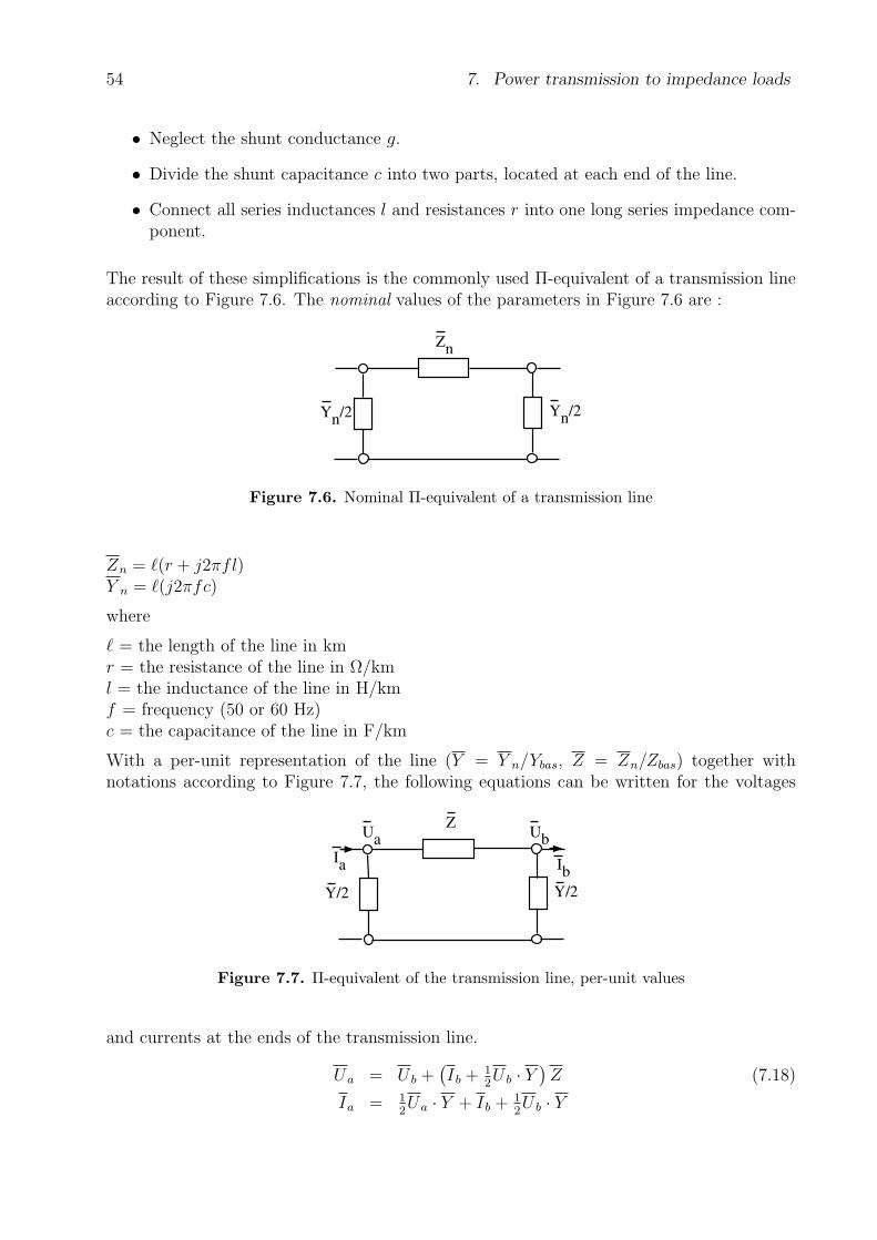
54 7. Power transmission to impedance loads
• Neglect the shunt conductance g.
• Divide the shunt capacitance c into two parts, located at each end of the line.
• Connect all series inductances l and resistances r into one long series impedance com-ponent.
The result of these simplifications is the commonly used Π-equivalent of a transmission lineaccording to Figure 7.6. The nominal values of the parameters in Figure 7.6 are :
Yn
/2Yn
/2
Zn
Figure 7.6. Nominal Π-equivalent of a transmission line
Zn = `(r + j2πfl)Y n = `(j2πfc)
where
` = the length of the line in kmr = the resistance of the line in Ω/kml = the inductance of the line in H/kmf = frequency (50 or 60 Hz)c = the capacitance of the line in F/km
With a per-unit representation of the line (Y = Y n/Ybas, Z = Zn/Zbas) together withnotations according to Figure 7.7, the following equations can be written for the voltages
Y/2Y/2
Z U
b
Ib
Ua
Ia
Figure 7.7. Π-equivalent of the transmission line, per-unit values
and currents at the ends of the transmission line.
Ua = U b +(Ib + 1
2U b · Y
)Z (7.18)
Ia = 12Ua · Y + Ib + 1
2U b · Y
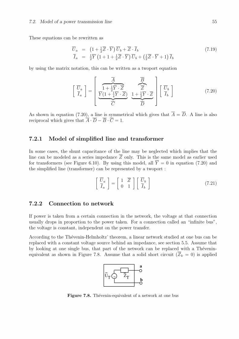
7.2. Model of a power transmission line 55
These equations can be rewritten as
Ua =(1 + 1
2Z · Y )
U b + Z · Ib (7.19)
Ia = 12Y
(1 + 1 + 1
2Z · Y )
U b +(
12Z · Y + 1
)Ib
by using the matrix notation, this can be written as a twoport equation
[Ua
Ia
]=
A︷ ︸︸ ︷1 + 1
2Y · Z
B︷︸︸︷Z
Y (1 + 14Y · Z)︸ ︷︷ ︸
C
1 + 12Y · Z︸ ︷︷ ︸
D
[U b
Ib
](7.20)
As shown in equation (7.20), a line is symmetrical which gives that A = D. A line is alsoreciprocal which gives that A ·D −B · C = 1.
7.2.1 Model of simplified line and transformer
In some cases, the shunt capacitance of the line may be neglected which implies that theline can be modeled as a series impedance Z only. This is the same model as earlier usedfor transformers (see Figure 6.10). By using this model, all Y = 0 in equation (7.20) andthe simplified line (transformer) can be represented by a twoport :
[Ua
Ia
]=
[1 Z0 1
] [U b
Ib
](7.21)
7.2.2 Connection to network
If power is taken from a certain connection in the network, the voltage at that connectionusually drops in proportion to the power taken. For a connection called an “infinite bus”,the voltage is constant, independent on the power transfer.
According to the Thevenin-Helmholtz’ theorem, a linear network studied at one bus can bereplaced with a constant voltage source behind an impedance, see section 5.5. Assume thatby looking at one single bus, that part of the network can be replaced with a Thevenin-equivalent as shown in Figure 7.8. Assume that a solid short circuit (Zk = 0) is applied
~ ZT
UT
a
b
Figure 7.8. Thevenin-equivalent of a network at one bus
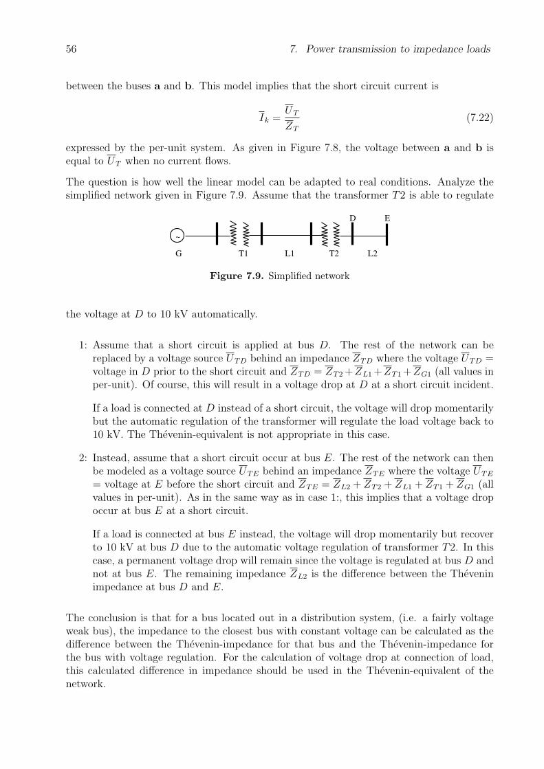
56 7. Power transmission to impedance loads
between the buses a and b. This model implies that the short circuit current is
Ik =UT
ZT
(7.22)
expressed by the per-unit system. As given in Figure 7.8, the voltage between a and b isequal to UT when no current flows.
The question is how well the linear model can be adapted to real conditions. Analyze thesimplified network given in Figure 7.9. Assume that the transformer T2 is able to regulate
~
G T1 L1 T2 L2
D E
Figure 7.9. Simplified network
the voltage at D to 10 kV automatically.
1: Assume that a short circuit is applied at bus D. The rest of the network can bereplaced by a voltage source UTD behind an impedance ZTD where the voltage UTD =voltage in D prior to the short circuit and ZTD = ZT2 +ZL1 +ZT1 +ZG1 (all values inper-unit). Of course, this will result in a voltage drop at D at a short circuit incident.
If a load is connected at D instead of a short circuit, the voltage will drop momentarilybut the automatic regulation of the transformer will regulate the load voltage back to10 kV. The Thevenin-equivalent is not appropriate in this case.
2: Instead, assume that a short circuit occur at bus E. The rest of the network can thenbe modeled as a voltage source UTE behind an impedance ZTE where the voltage UTE
= voltage at E before the short circuit and ZTE = ZL2 + ZT2 + ZL1 + ZT1 + ZG1 (allvalues in per-unit). As in the same way as in case 1:, this implies that a voltage dropoccur at bus E at a short circuit.
If a load is connected at bus E instead, the voltage will drop momentarily but recoverto 10 kV at bus D due to the automatic voltage regulation of transformer T2. In thiscase, a permanent voltage drop will remain since the voltage is regulated at bus D andnot at bus E. The remaining impedance ZL2 is the difference between the Theveninimpedance at bus D and E.
The conclusion is that for a bus located out in a distribution system, (i.e. a fairly voltageweak bus), the impedance to the closest bus with constant voltage can be calculated as thedifference between the Thevenin-impedance for that bus and the Thevenin-impedance forthe bus with voltage regulation. For the calculation of voltage drop at connection of load,this calculated difference in impedance should be used in the Thevenin-equivalent of thenetwork.

7.2. Model of a power transmission line 57
In some cases, the term short circuit capacity Sk at a bus in the network, is used. It isdefined as
Sk = UT I∗k (7.23)
hence it follows that this is the power that is obtained in the Thevenin-impedance. Sincethis impedance often is mostly reactive, the angle of the power that is obtained is close to+90. The short circuit capacity is of interest when the loadability of a certain bus is askedfor. The short circuit capacity indicates how much the bus voltage will change for differentmagnitudes of bus loading. The voltage increase at generator buses can also be calculated.
Example 7.1 At a bus with a short circuit capacity of 500 MVA and cos φk = 0, inductive,an impedance load of 4 MW, cos φLD = 0.8 at nominal voltage, is connected. Calculate thechange in bus voltage when the load is connected.
Solution
Assume a voltage of 1 pu and a base power Sb = 500 MVA. The network can then be modeledas given in Figure 7.10.
~
ZTpu
UT
= 1pu ZLDpu
U’LD
Figure 7.10. Single-phase model of system given in example
The Thevenin-impedance can be calculated according to equation (7.22) and (7.23) :
ZT−pu =UT
Ik
=U2
T
S∗k
=1
16 − 90= j1 (7.24)
The load impedance can be calculated as
ZLD−pu = (U2LD−pu/S
∗LD−pu) = (1/[4/(500 · 0.8)])(0.8 + j0.6) = 80 + j60 (7.25)
By a simple voltage division, the voltage U′LD at the load can be calculated as
U′LD =
UT ZLD−pu
ZT−pu + ZLD−pu
=1 · (80 + j60)
j1 + 80 + j60= 0.9940 6 − 0.4556 (7.26)
i.e. the voltage drop is about 0.6 %.
Conclusion : A load with an apparent power of 1 % of the short circuit capacity at the busconnected, will cause a voltage drop at that bus of ≈ 1 %.

58 7. Power transmission to impedance loads
Example 7.2 A small industry is fed by a transformer (5 MVA, 70/10 kV, x = 4 %) whichis located at a distance of 5 km. The electric power demand of the industry is 400 kW atcosφ=0.8, lagging, at a voltage of 10 kV. The industry can be modeled as an impedance load.The 10 kV line has an series impedance of 0.9+j0.3 Ω/phase,km and a shunt admittanceof j3 × 10−6 S/phase,km. Assume that the line is modeled by the Π-equivalent. Calculatethe voltage level at the industry as well as the power fed by the transformer into the line.When the industry is not connected, a short circuit current of 0.3 kA, pure inductive, can beobtained on the 70 kV side of the transformer when a three-phase short circuit is applied atnominal voltage.
Solution
Chose base values (MVA, kV, ⇒ kA, Ω) : Sb = 500 kVA = 0.5 MVA, Ub10 = 10 kV
Power system Transformer Line Industry
Figure 7.11. Power system used in example 7.2
⇒ Ib10 = Sb/√
3Ub10 = 0.0289 kA, Zb10 = U2b10/Sb = 200 Ω, Ub70 = 70 kV ⇒ Ib70 =
Sb/√
3Ub70 = 0.0041 kA
Calculate the per-unit values of the Thevenin-equivalent of the system :Equation (7.22) ⇒ ZTh = UTh/Ik ⇒ ZThpu = (UTh/Ub70) · (Ib70/Ik) = (70 6 0/70) ·(0.00412/0.36 − 90) = j0.0137, UThpu = UTh/Ub70 = 1.06 0
Calculate the per-unit values of the transformer :Ztrapu = (Ztra%/100) · Zbtra70/Zb70 = (Ztra%/100) · Sb/Stra = (j4/100) · 0.5/5 = j0.004
Calculate the per-unit values of the line :Z lpu = 5 · [0.9 + j0.3]/Zb10 = 0.0225 + j0.0075Y lpu = 5 · [j3× 10−6]/Yb10 = 5 · [j3× 10−6] · Zb10 = j0.003AL = 1 + 1
2Y lpu · Z lpu = 1.0000 + j0.0000
BL = Z lpu = 0.0225 + j0.0075CL = Y lpu(1 + 1
4Y lpu · Z lpu) = 0.0000 + j0.0030
DL = AL = 1.0000 + j0.0000
Calculate the per-unit values of the industry impedance :Zindpu = (U2
ind/S∗ind)/Zb10 = (102/[0.4/0.8]) · (0.8 + j0.6)/200 = 0.8 + j0.6
The twoport of the whole system between the “infinite bus” and the industry, (power system
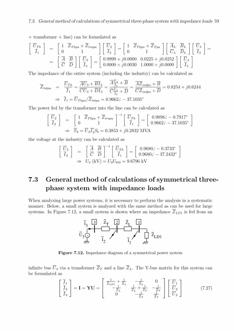
7.3. General method of calculations of symmetrical three-phase system with impedance loads 59
+ transformer + line) can be formulated as[
UTh
I1
]=
[1 ZThpu + Ztrapu
0 1
] [U2
I2
]=
[1 ZThpu + ZTpu
0 1
] [AL BL
CL DL
] [U3
I3
]=
=
[A BC D
] [U3
I3
]=
[0.9999 + j0.0000 0.0225 + j0.02520.0000 + j0.0030 1.0000 + j0.0000
] [U3
I3
]
The impedance of the entire system (including the industry) can be calculated as
Ztotpu =UTh
I1
=AU3 + BI3
CU3 + DI3
=AU3
I3+ B
C U3
I3+ D
=AZindpu + B
CZindpu + D= 0.8254 + j0.6244
⇒ I1 = UThpu/Ztotpu = 0.96626 − 37.1035
The power fed by the transformer into the line can be calculated as[
U2
I2
]=
[1 ZThpu + Ztrapu
0 1
]−1 [UTh
I1
]=
[0.98986 − 0.7917
0.9662 6 − 37.1035
]
⇒ S2 = U2I∗2Sb = 0.3853 + j0.2832 MVA
the voltage at the industry can be calculated as[
U3
I3
]=
[A BC D
]−1 [UTh
I1
]=
[0.9680 6 − 0.3733
0.96806 − 37.2432
]
⇒ U3 (kV) = U3Ub10 = 9.6796 kV
7.3 General method of calculations of symmetrical three-
phase system with impedance loads
When analyzing large power systems, it is necessary to perform the analysis in a systematicmanner. Below, a small system is analyzed with the same method as can be used for largesystems. In Figure 7.12, a small system is shown where an impedance ZLD1 is fed from an
~
2 13
ZLD1
ZL
ZT
U3
I2 I
1
I3
Figure 7.12. Impedance diagram of a symmetrical power system
infinite bus U3 via a transformer ZT and a line ZL. The Y-bus matrix for this system canbe formulated as
I1
I2
I3
= I = YU =
1ZLD1
+ 1ZL
− 1ZL
0
− 1ZL
1ZL
+ 1ZT
− 1ZT
0 − 1ZT
1ZT
U1
U2
U3
(7.27)
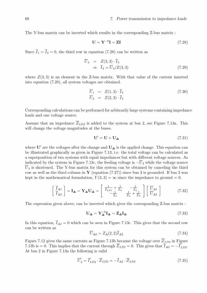
60 7. Power transmission to impedance loads
The Y-bus matrix can be inverted which results in the corresponding Z-bus matrix :
U = Y−1I = ZI (7.28)
Since I1 = I2 = 0, the third row in equation (7.28) can be written as
U3 = Z(3, 3) · I3
⇒ I3 = U3/Z(3, 3) (7.29)
where Z(3, 3) is an element in the Z-bus matrix. With that value of the current insertedinto equation (7.28), all system voltages are obtained.
U1 = Z(1, 3) · I3 (7.30)
U2 = Z(2, 3) · I3
Corresponding calculations can be performed for arbitrarily large systems containing impedanceloads and one voltage source.
Assume that an impedance ZLD2 is added to the system at bus 2, see Figure 7.13a. Thiswill change the voltage magnitudes at the buses.
U′ = U + U∆ (7.31)
where U′ are the voltages after the change and U∆ is the applied change. This equation canbe illustrated graphically as given in Figure 7.13, i.e. the total voltage can be calculated asa superposition of two systems with equal impedances but with different voltage sources. Asindicated by the system in Figure 7.13c, the feeding voltage is −U2 while the voltage sourceU3 is shortened. The Y-bus matrix for this system can be obtained by canceling the thirdrow as well as the third column in Y (equation (7.27)) since bus 3 is grounded. If bus 3 waskept in the mathematical formulation, Y (3, 3) = ∞ since the impedance to ground = 0.
[I∆1
I∆2
]= I∆ = Y∆U∆ =
[1
ZLD1+ 1
ZL− 1
ZL− 1ZL
1ZL
+ 1ZT
][U∆1
U∆2
](7.32)
The expression given above, can be inverted which gives the corresponding Z-bus matrix :
U∆ = Y−1∆ I∆ = Z∆I∆ (7.33)
In this equation, I∆1 = 0 which can be seen in Figure 7.13c. This gives that the second rowcan be written as
U∆2 = Z∆(2, 2)I∆2 (7.34)
Figure 7.12 gives the same currents as Figure 7.13b because the voltage over ZLD2 in Figure7.13b is = 0. This implies that the current through ZLD2 = 0. This gives that I∆2 = −I
′LD2.
At bus 2 in Figure 7.13a the following is valid
U′2 = I
′LD2 · ZLD2 = −I∆2 · ZLD2 (7.35)

7.3. General method of calculations of symmetrical three-phase system with impedance loads 61
~
2 13
ZLD1
ZL
ZT
U3
~
2 13
ZLD1
ZL
ZT
U3
~+U2
ZLD2
ILD2
=0
=
+
c)
b)
a) U’
U
U∆
2 1
ZLD1
ZL
ZT
~ U2
ZLD2
I∆2= I’
LD2
I∆1=0
ZLD2
I’LD2
Figure 7.13. Total voltage obtained by using superposition
By combining equation (7.31), (7.34) and (7.35), the following can be obtained
I∆2 =−U2
ZLD2 + Z∆(2, 2)(7.36)
By inserting that value in the equations given above, all voltages after the system changecan be calculated as :
U′2 =
ZLD2
ZLD2 + Z∆(2, 2)U2 (7.37)
U′1 = U1 − Z∆(1, 2)
ZLD2 + Z∆(2, 2)U2 (7.38)
The procedure given above can be generalized to be used for an arbitrarily large system.Assume that the impedance Zr is connected to bus r and an arbitrary bus is named i. Thecurrent Ir (=−I∆r) through Zr can be calculated as well as the voltages after connection of

62 7. Power transmission to impedance loads
the impedance Zr at bus r. The equations are as follows.
Ir =U r
Zr + Z∆(r, r)(7.39)
U′r =
Zr
Zr + Z∆(r, r)U r (7.40)
U′i = U i − Z∆(i, r)
Zr + Z∆(r, r)U r i 6= r (7.41)
The Thevenin-equivalent at a bus in a symmetrical network can be calculated by usingequations (7.31) and (7.33). At bus r (r=2 in these equations), the equation will be as
U′(r) = U(r) + Z∆(r, r)I∆r (7.42)
where
U(r) = Thevenin-voltage at bus r, see Figure 7.14.
Z∆(r, r) = Thevenin-impedance at bus r, see Figure 7.14.
I∆r = The current that is injected into bus r.
U′(r) = the voltage at bus r.
o
o
~
Z∆(r,r)U’(r)
U(r)I∆r
Figure 7.14. Thevenin-equivalent at bus r in a symmetrical three-phase network
As given by equation (7.42) and Figure 7.14, U′(r) = U(r) when I∆r = 0. This formulationshows that the Thevenin-voltage at bus r can be calculated as the voltage at bus r whenthe bus is not loaded, i.e. I∆r = 0. The Thevenin-impedance can be calculated as the r-thdiagonal element in the impedance matrix Z∆. The matrix is calculated with all voltagesources shortened.
Example 7.3 In Figure 7.15, an internal network of an industry is given. The energy isdelivered by an infinite bus with a nominal voltage at bus 1. The energy is transmitted viatransformer T1, line L2 and transformer T2 to the load LD2. There is also a high voltageload LD1 connected to T1 via the line L1. Ratings of the different components are :
• Transformer T1 : 800 kVA, 70/10 kV, x = 7 %
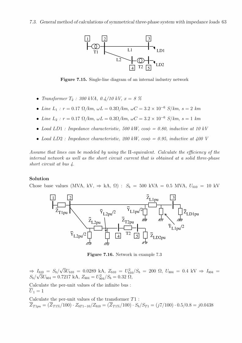
7.3. General method of calculations of symmetrical three-phase system with impedance loads 63
1 2 3
54
L1
L2
T1
T2
LD1
LD2
Figure 7.15. Single-line diagram of an internal industry network
• Transformer T2 : 300 kVA, 0.4/10 kV, x = 8 %
• Line L1 : r = 0.17 Ω/km, ωL = 0.3Ω/km, ωC = 3.2× 10⁻⁶ S/km, s = 2 km
• Line L2 : r = 0.17 Ω/km, ωL = 0.3Ω/km, ωC = 3.2× 10⁻⁶ S/km, s = 1 km
• Load LD1 : Impedance characteristic, 500 kW, cosφ = 0.80, inductive at 10 kV
• Load LD2 : Impedance characteristic, 200 kW, cosφ = 0.95, inductive at 400 V
Assume that lines can be modeled by using the Π-equivalent. Calculate the efficiency of theinternal network as well as the short circuit current that is obtained at a solid three-phaseshort circuit at bus 4.
Solution
Chose base values (MVA, kV, ⇒ kA, Ω) : Sb = 500 kVA = 0.5 MVA, Ub10 = 10 kV
1 2 3
54
ZL1pu
ZT1pu
T2
YL1pu/2
ZL2pu
YL2pu/2
ZT2pu
ZLD2pu
ZLD1pu
YL1pu/2
YL2pu/2
Figure 7.16. Network in example 7.3
⇒ Ib10 = Sb/√
3Ub10 = 0.0289 kA, Zb10 = U2b10/Sb = 200 Ω, Ub04 = 0.4 kV ⇒ Ib04 =
Sb/√
3Ub04 = 0.7217 kA, Zb04 = U2b04/Sb = 0.32 Ω,
Calculate the per-unit values of the infinite bus :U1 = 1
Calculate the per-unit values of the transformer T1 :ZT1pu = (ZT1%/100) · ZbT1−10/Zb10 = (ZT1%/100) · Sb/ST1 = (j7/100) · 0.5/0.8 = j0.0438
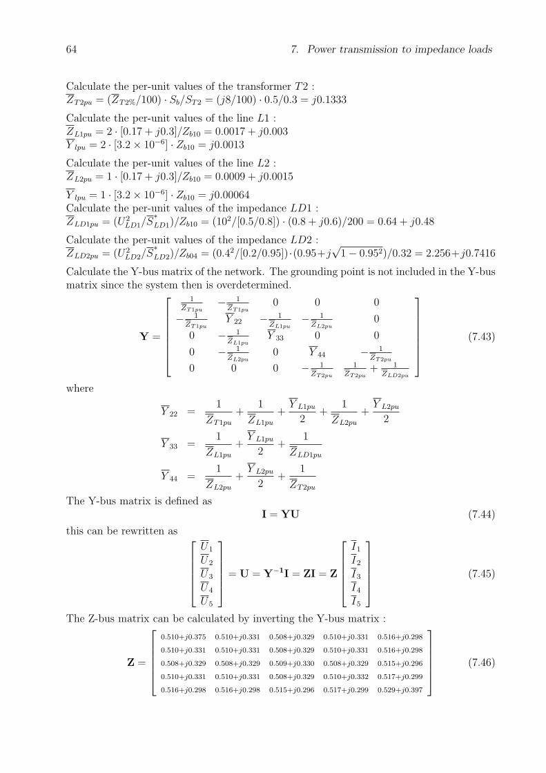
64 7. Power transmission to impedance loads
Calculate the per-unit values of the transformer T2 :ZT2pu = (ZT2%/100) · Sb/ST2 = (j8/100) · 0.5/0.3 = j0.1333
Calculate the per-unit values of the line L1 :ZL1pu = 2 · [0.17 + j0.3]/Zb10 = 0.0017 + j0.003Y lpu = 2 · [3.2× 10−6] · Zb10 = j0.0013
Calculate the per-unit values of the line L2 :ZL2pu = 1 · [0.17 + j0.3]/Zb10 = 0.0009 + j0.0015
Y lpu = 1 · [3.2× 10−6] · Zb10 = j0.00064Calculate the per-unit values of the impedance LD1 :ZLD1pu = (U2
LD1/S∗LD1)/Zb10 = (102/[0.5/0.8]) · (0.8 + j0.6)/200 = 0.64 + j0.48
Calculate the per-unit values of the impedance LD2 :ZLD2pu = (U2
LD2/S∗LD2)/Zb04 = (0.42/[0.2/0.95])·(0.95+j
√1− 0.952)/0.32 = 2.256+j0.7416
Calculate the Y-bus matrix of the network. The grounding point is not included in the Y-busmatrix since the system then is overdetermined.
Y =
1ZT1pu
− 1ZT1pu
0 0 0
− 1ZT1pu
Y 22 − 1ZL1pu
− 1ZL2pu
0
0 − 1ZL1pu
Y 33 0 0
0 − 1ZL2pu
0 Y 44 − 1ZT2pu
0 0 0 − 1ZT2pu
1ZT2pu
+ 1ZLD2pu
(7.43)
where
Y 22 =1
ZT1pu
+1
ZL1pu
+Y L1pu
2+
1
ZL2pu
+Y L2pu
2
Y 33 =1
ZL1pu
+Y L1pu
2+
1
ZLD1pu
Y 44 =1
ZL2pu
+Y L2pu
2+
1
ZT2pu
The Y-bus matrix is defined asI = YU (7.44)
this can be rewritten as
U1
U2
U3
U4
U5
= U = Y−1I = ZI = Z
I1
I2
I3
I4
I5
(7.45)
The Z-bus matrix can be calculated by inverting the Y-bus matrix :
Z =
0.510+j0.375 0.510+j0.331 0.508+j0.329 0.510+j0.331 0.516+j0.298
0.510+j0.331 0.510+j0.331 0.508+j0.329 0.510+j0.331 0.516+j0.298
0.508+j0.329 0.508+j0.329 0.509+j0.330 0.508+j0.329 0.515+j0.296
0.510+j0.331 0.510+j0.331 0.508+j0.329 0.510+j0.332 0.517+j0.299
0.516+j0.298 0.516+j0.298 0.515+j0.296 0.517+j0.299 0.529+j0.397
(7.46)
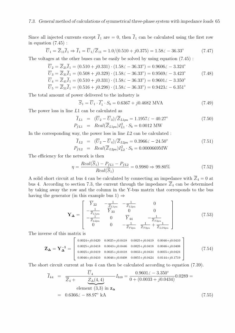
7.3. General method of calculations of symmetrical three-phase system with impedance loads 65
Since all injected currents except I1 are = 0, then I1 can be calculated using the first rowin equation (7.45) :
U1 = Z11I1 ⇒ I1 = U1/Z11 = 1.0/(0.510 + j0.375) = 1.586 − 36.33 (7.47)
The voltages at the other buses can be easily be solved by using equation (7.45) :
U2 = Z21I1 = (0.510 + j0.331) · (1.58 6 − 36.33) = 0.9606 6 − 3.324
U3 = Z31I1 = (0.508 + j0.329) · (1.58 6 − 36.33) = 0.9569 6 − 3.423 (7.48)
U4 = Z41I1 = (0.510 + j0.331) · (1.58 6 − 36.33) = 0.9601 6 − 3.350
U5 = Z51I1 = (0.516 + j0.298) · (1.58 6 − 36.33) = 0.9423 6 − 6.351
The total amount of power delivered to the industry is
S1 = U1 · I∗1 · Sb = 0.6367 + j0.4682 MVA (7.49)
The power loss in line L1 can be calculated as
IL1 = (U2 − U3)/ZL1pu = 1.1957 6 − 40.27 (7.50)
PfL1 = Real(ZL1pu)I2L1 · Sb = 0.0012 MW
In the corresponding way, the power loss in line L2 can be calculated :
IL2 = (U2 − U4)/ZL2pu = 0.3966 6 − 24.50 (7.51)
PfL2 = Real(ZL2pu)I2L2 · Sb = 0.0000669MW
The efficiency for the network is then
η =Real(S1)− PfL1 − PfL2
Real(S1)= 0.9980 ⇒ 99.80% (7.52)
A solid short circuit at bus 4 can be calculated by connecting an impedance with Z4 = 0 atbus 4. According to section 7.3, the current through the impedance Z4 can be determinedby taking away the row and the column in the Y-bus matrix that corresponds to the bushaving the generator (in this example bus 1) ⇒
Y∆ =
Y 22 − 1ZL1pu
− 1ZL2pu
0
− 1ZL1pu
Y 33 0 0
− 1ZL2pu
0 Y 44 − 1ZT2pu
0 0 − 1ZT2pu
1ZT2pu
+ 1ZLD2pu
(7.53)
The inverse of this matrix is
Z∆ = Y−1∆ =
0.0024+j0.0420 0.0025+j0.0418 0.0025+j0.0419 0.0046+j0.0410
0.0025+j0.0418 0.0043+j0.0446 0.0025+j0.0418 0.0046+j0.0408
0.0025+j0.0419 0.0025+j0.0418 0.0033+j0.0434 0.0055+j0.0424
0.0046+j0.0410 0.0046+j0.0408 0.0055+j0.0424 0.0144+j0.1719
(7.54)
The short circuit current at bus 4 can then be calculated according to equation (7.39).
Ik4 =U4
Z4 + Z∆(4, 4)︸ ︷︷ ︸element (3,3) in Z∆
Ib10 =0.9601 6 − 3.350
0 + (0.0033 + j0.0434)0.0289 =
= 0.6366 6 − 88.97 kA (7.55)

66 7. Power transmission to impedance loads
7.4 Extended method to be used for power loads
The method described in section 7.3 is valid when all system load are modeled as impedanceload, i.e. the power consumed is proportional to the voltage squared. In steady-state con-ditions, an often used load model is the constant power model. The method described insection 7.3 can be used in an iterative way, described in the following :
1. Calculate the per-unit values of all components that are of interest. Loads thatare modeled with constant power (independent of the voltage) are replaced by animpedance under the assumption that nominal voltage apply. The impedance of aload at bus k can be calculated as ZLDk = U2
k/S∗LDk where Uk = 1 pu, and SLDk is
the rated power of the load.
2. Calculate the Y-bus matrix and the corresponding Z-bus matrix of the network as wellas the load impedances. By using the method described in section 7.3 (equation (7.29)and (7.30)), the voltage at all buses can be calculated.
3. Calculate the load demand at all loads. The power demand SLDk−b at load LDk isobtained as SLDk−b = U2
k/Z∗LDk where Uk is the calculated voltage at bus k.
4. Calculate the difference between calculated and specified load demand for all powerloads :
∆PLDk = |Re(SLDk−b)−Re(SLDk)| (7.56)
∆QLDk = |Im(SLDk−b)− Im(SLDk)| (7.57)
5. If ∆PLDk and/or ∆QLDk are too large for a certain bus :
(a) Calculate new load impedances according to ZLDk = U2k/S
∗LDk where Uk is the
most recent estimation of the voltage at bus k.
(b) Go back to item #2 and repeat the calculations
If ∆PLDk and ∆QLDk are found to be acceptable for all power loads, the iterationprocess is finished.
A simple example will be given to clarify this method.
Example 7.4 Assume a line operating with a voltage of U1 = 225 6 0 kV in the sendingend, and with a load of PD2 = 80 MW and QD2 = 60 MVAr in the receiving end. The linehas a length of 100 km and has x = 0.4 Ω/km, r = 0.04 Ω/km and b = 3 × 10⁻⁶ S/km.Calculate the receiving end voltage.
Solution
In Figure 7.17, the network modeled by impedance loads is given.
Assume Sb = 100 MVA and Ub = 225 kV which gives
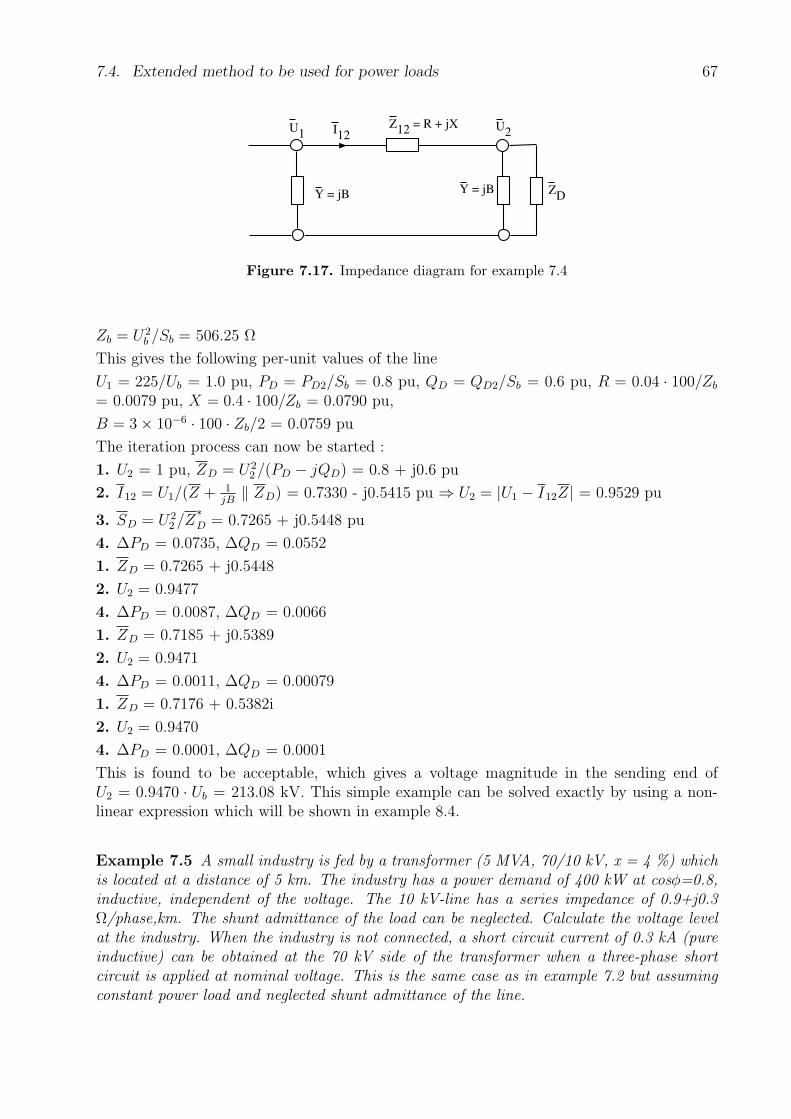
7.4. Extended method to be used for power loads 67
U1Z12 = R + jX U2I12
Y = jB Y = jB ZD
Figure 7.17. Impedance diagram for example 7.4
Zb = U2b /Sb = 506.25 Ω
This gives the following per-unit values of the line
U1 = 225/Ub = 1.0 pu, PD = PD2/Sb = 0.8 pu, QD = QD2/Sb = 0.6 pu, R = 0.04 · 100/Zb
= 0.0079 pu, X = 0.4 · 100/Zb = 0.0790 pu,
B = 3× 10−6 · 100 · Zb/2 = 0.0759 pu
The iteration process can now be started :
1. U2 = 1 pu, ZD = U22 /(PD − jQD) = 0.8 + j0.6 pu
2. I12 = U1/(Z + 1jB‖ ZD) = 0.7330 - j0.5415 pu ⇒ U2 = |U1 − I12Z| = 0.9529 pu
3. SD = U22 /Z
∗D = 0.7265 + j0.5448 pu
4. ∆PD = 0.0735, ∆QD = 0.0552
1. ZD = 0.7265 + j0.5448
2. U2 = 0.9477
4. ∆PD = 0.0087, ∆QD = 0.0066
1. ZD = 0.7185 + j0.5389
2. U2 = 0.9471
4. ∆PD = 0.0011, ∆QD = 0.00079
1. ZD = 0.7176 + 0.5382i
2. U2 = 0.9470
4. ∆PD = 0.0001, ∆QD = 0.0001
This is found to be acceptable, which gives a voltage magnitude in the sending end ofU2 = 0.9470 · Ub = 213.08 kV. This simple example can be solved exactly by using a non-linear expression which will be shown in example 8.4.
Example 7.5 A small industry is fed by a transformer (5 MVA, 70/10 kV, x = 4 %) whichis located at a distance of 5 km. The industry has a power demand of 400 kW at cosφ=0.8,inductive, independent of the voltage. The 10 kV-line has a series impedance of 0.9+j0.3Ω/phase,km. The shunt admittance of the load can be neglected. Calculate the voltage levelat the industry. When the industry is not connected, a short circuit current of 0.3 kA (pureinductive) can be obtained at the 70 kV side of the transformer when a three-phase shortcircuit is applied at nominal voltage. This is the same case as in example 7.2 but assumingconstant power load and neglected shunt admittance of the line.
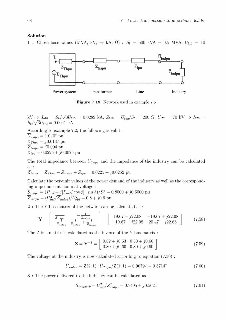
68 7. Power transmission to impedance loads
Solution
1 : Chose base values (MVA, kV, ⇒ kA, Ω) : Sb = 500 kVA = 0.5 MVA, Ub10 = 10
Power system Transformer Line Industry
Figure 7.18. Network used in example 7.5
kV ⇒ Ib10 = Sb/√
3Ub10 = 0.0289 kA, Zb10 = U2b10/Sb = 200 Ω, Ub70 = 70 kV ⇒ Ib70 =
Sb/√
3Ub70 = 0.0041 kA
According to example 7.2, the following is valid :UThpu = 1.0 6 0 puZThpu = j0.0137 puZtrapu = j0.004 puZ lpu = 0.0225 + j0.0075 pu
The total impedance between UThpu and the impedance of the industry can be calculatedas :Ztotpu = ZThpu + Ztrapu + Z lpu = 0.0225 + j0.0252 pu
Calculate the per-unit values of the power demand of the industry as well as the correspond-ing impedance at nominal voltage :Sindpu = (Pind + j[Pind/ cos φ] · sin φ)/Sb = 0.8000 + j0.6000 pu
Zindpu = (U2ind/S
∗indpu)/U
2b10 = 0.8 + j0.6 pu
2 : The Y-bus matrix of the network can be calculated as :
Y =
[1
Ztotpu− 1
Ztotpu
− 1Ztotpu
1Ztotpu
+ 1Zindpu
]=
[19.67− j22.08 −19.67 + j22.08−19.67 + j22.08 20.47− j22.68
](7.58)
The Z-bus matrix is calculated as the inverse of the Y-bus matrix :
Z = Y−1 =
[0.82 + j0.63 0.80 + j0.600.80 + j0.60 0.80 + j0.60
](7.59)
The voltage at the industry is now calculated according to equation (7.30) :
U indpu = Z(2, 1) · UThpu/Z(1, 1) = 0.9679 6 − 0.3714 (7.60)
3 : The power delivered to the industry can be calculated as :
Sindpu−b = U2ind/Z
∗indpu = 0.7495 + j0.5621 (7.61)
7.4. Extended method to be used for power loads 69
4 : The difference between calculated and specified power can be calculated as :
∆Pind = |Re(Sindpu−b)−Re(Sindpu)| = 0.0505 (7.62)
∆Qind = |Im(Sindpu−b)− Im(Sindpu)| = 0.0379 (7.63)
5 : These deviations are too large and the calculations are therefore repeated and a newindustry impedance is calculated by using the new voltage magnitude :
Zindpu = (U2indpu/S
∗indpu) = 0.7495 + j0.5621 (7.64)
Repeat the calculations from item #2.
2, 3 : ⇒ Sindpu−b = 0.7965 + j0.59744 : ∆Pind = 0.0035, ∆Qind = 0.0026Unacceptable ⇒5 : Zindpu = 0.7462 + j0.5597Continue from item #2.
2, 3 : ⇒ Sindpu−b = 0.7998 + j0.59984 : ∆Pind = 0.00024, ∆Qind = 0.00018Unacceptable ⇒5 : Zindpu = 0.7460 + j0.5595Continue from item #2.
2, 3 : ⇒ Sindpu−b = 0.8000 + j0.60004 : ∆Pind = 0.000016, ∆Qind = 0.000012Acceptable ⇒U ind = U indpu · Ub10 = 9.6565 6 − 0.3974

70 7. Power transmission to impedance loads
Chapter 8
Non-linear static analysis
In chapter 6–7, two assumptions were made: firstly, the network has had only one generationbus, secondly, the loads have been modeled by impedances. The assumptions made gave asystem that could be modeled by using a linear set of equations which can be solved quiteeasily.
In the following, these assumptions are not valid, i.e. the loads will be modeled as con-stant power loads and power can be generated at more than one location. First, the powertransmission on an overhead line will be studied, followed by a more general system analysis.
8.1 Power flow on a line
Power lines can be modeled in several different ways depending on what parameters thatcan be considered as known and on the purpose of the system analysis. This leads to severaldifferent expressions on power flows on lines. The voltages are given by polar representation,i.e. voltage magnitude and angle as
Uk = Ukejθk (8.1)
U j = Ujejθj (8.2)
where the phase angle difference between two buses has the following notation
θkj = θk − θj (8.3)
In the following, the shunt admittance of the line is neglected.
8.1.1 Line model with rectangular series impedance
The model presented here models a line with a π-equivalent with the series impedance givenon rectangular form as given in Figure 8.1. The rectangular form means that the seriesimpedance is given in one resistive part R and in one reactive part X as
Zkj = R + jX |Zkj| = Z =√
R2 + X2 (8.4)
The power Skj in the sending end k can be calculated by using the per-unit system as
Skj = Uk
(I∗kj0 + I
∗kj
)= Uk
(U∗kY
∗+
U∗k − U
∗j
Z∗kj
)= (8.5)
= U2k (−jB) +
U2k
R− jX− UkUj
R− jXej(θk−θj) =
= U2k (−jB) +
U2k
Z2(R + jX)− UkUj
Z2(R + jX) (cos θkj + j sin θkj)
71
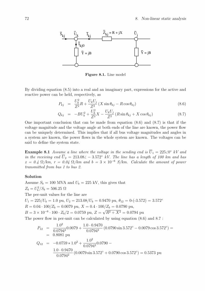
72 8. Non-linear static analysis
SkjUk
Zkj = R + jX Uj
Ikj0
Ikj
Y = jB Y = jB
Figure 8.1. Line model
By dividing equation (8.5) into a real and an imaginary part, expressions for the active andreactive power can be held, respectively, as
Pkj =U2
k
Z2R +
UkUj
Z2(X sin θkj −R cos θkj) (8.6)
Qkj = −BU2k +
U2k
Z2X − UkUj
Z2(R sin θkj + X cos θkj) (8.7)
One important conclusion that can be made from equation (8.6) and (8.7) is that if thevoltage magnitude and the voltage angle at both ends of the line are known, the power flowcan be uniquely determined. This implies that if all bus voltage magnitudes and angles ina system are known, the power flows in the whole system are known. The voltages can besaid to define the system state.
Example 8.1 Assume a line where the voltage in the sending end is U1 = 225 6 0 kV andin the receiving end U2 = 213.086 − 3.572 kV. The line has a length of 100 km and hasx = 0.4 Ω/km, r = 0.04 Ω/km and b = 3 × 10⁻⁶ S/km. Calculate the amount of powertransmitted from bus 1 to bus 2.
Solution
Assume Sb = 100 MVA and Ub = 225 kV, this gives that
Zb = U2b /Sb = 506.25 Ω
The per-unit values for the line are
U1 = 225/Ub = 1.0 pu, U2 = 213.08/Ub = 0.9470 pu, θ12 = 0-(-3.572) = 3.572
R = 0.04 · 100/Zb = 0.0079 pu, X = 0.4 · 100/Zb = 0.0790 pu,
B = 3× 10−6 · 100 · Zb/2 = 0.0759 pu, Z =√
R2 + X2 = 0.0794 pu
The power flow in per-unit can be calculated by using equation (8.6) and 8.7 :
P12 =1.02
0.079420.0079 +
1.0 · 0.9470
0.07942(0.0790 sin 3.572 − 0.0079 cos 3.572) =
= 0.8081 pu
Q12 = −0.0759 ∗ 1.02 +1.02
0.079420.0790−
1.0 · 0.9470
0.07942(0.0079 sin 3.572 + 0.0790 cos 3.572) = 0.5373 pu
8.1. Power flow on a line 73
expressed in nominal values
P12 = 0.8081 · Sb = 80.81 MW
Q12 = 0.5373 · Sb = 53.73 MVAr
For this simple system, the calculations can be performed without using the per-unit system.By using equation (6.6), equation (8.6) can be rewritten as
Pkj(MW) = Pkj(pu)Sb =U2
b
Zb
U2
k
Z2R +
UkUj
Z2(X sin θkj −R cos θkj)
=
=U2
k (kV)
Z2(Ω)R(Ω) +
Uk(kV) · Uj(kV)
Z2(Ω)(X(Ω) sin θkj −R(Ω) cos θkj)
i.e. this equation is the same independent on if the values are given as nominal or per-unitvalues.
For a high voltage overhead line (U > 70 kV), the line reactance is normally considerablyhigher than the resistance of the line, i.e. R ¿ X in equation (8.6). An approximate formof that equation is
Pkj ≈ UkUj
Xsin θkj (8.8)
i.e. the sign of θkj determines the direction of the active power flow on the line. Normally,the active power will flow towards the bus with the lowest voltage angle. This holds also forlines having a pronounced resistivity.
Assume that the voltages Uk and U j are in phase and that the reactance of the line is dom-inating the line resistance. This implies that the active power flow is very small. Equation(8.7) can be rewritten as
Qkj = −BU2k +
Uk(Uk − Uj)
X(8.9)
Equation (8.9) indicates that this type of line gives a reactive power flow towards the buswith the lowest voltage magnitude. The equation shows that if the difference in voltagemagnitude between the ends of the line is small, the line will generate reactive power. Thissince the reactive power generated by the shunt admittances in that case dominates thereactive power consumed by the series reactance. The “rule of thumb” that reactive powerflows towards the bus with lowest voltage is more vague than the rule that active powerflows towards the bus with lowest angle. The fact that overhead lines and especially cables,generates reactive power when the active power flow is low, is important to be aware of.
Example 8.2 Calculate the active and reactive power flows on the line in example 8.1, usingthe approximate expressions 8.8 and 8.9, respectively.
Solution
P12 ≈ 1.0 · 0.9470
0.0790sin 3.572 = 0.7468 pu ⇒ 74.68 MW
Q12 ≈ −0.0759 · 1.02 +1.0(1.0− 0.9470)
0.0790= 0.5948 pu ⇒ 59.48 MVAr
74 8. Non-linear static analysis
the answers are of right dimension and have correct direction of the power flow but the activepower flow is about 8 % too low and the reactive power flow is 11 % too large.
8.1.2 Losses on a line
The active power losses on a three-phase line are dependent on the line resistance and onethe actual line current. By using nominal values, the losses can be calculated as
Pf = 3RI2 (8.10)
The squared current dependence in equation (8.10) can be written as
I2 = Iej arg(I)Ie−j arg(I) = II∗
=S∗
√3U
∗S√3U
=S2
3U2=
P 2 + Q2
3U2(8.11)
The active power losses for the line given in Figure 8.1 can be calculated as
Pf = RP 2
kj + (Qkj + BU2k )2
U2k
(8.12)
where
BU2k = the reactive power generated by the shunt capacitance at bus k
The expression given by (8.12) is valid both for nominal and for per-unit values. Thisequation shows that a doubling of transmitted active power will increase the active powerlosses by a factor of four. If the voltage is doubled, the active power losses will decrease witha factor of four.
Assume that the active power injections at both ends of the line are known, i.e. both Pkj
and Pjk have been calculated using equation (8.6). The active power losses can then becalculated as
Pf = Pkj + Pjk (8.13)
The reactive power losses can be obtained in the corresponding manner
Qf = 3XI2 = XP 2
kj + (Qkj + BU2k )2
U2k
(8.14)
Equations (8.11) and (8.12) shows that the losses are proportional to S2 and that the losseswill increase if reactive power is transmitted over the line. A natural solution to that is togenerate the reactive power as close to the consumer as possible. Of course, active poweris also generated as close to the consumer as possible, but the generation costs are of greatimportance.
Example 8.3 Use the same line as in example 8.1 and calculate the active power losses.
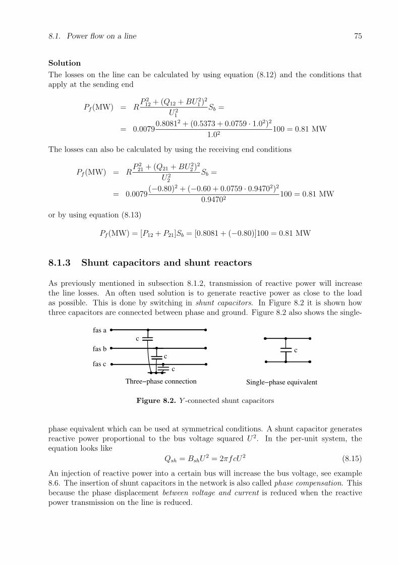
8.1. Power flow on a line 75
Solution
The losses on the line can be calculated by using equation (8.12) and the conditions thatapply at the sending end
Pf (MW) = RP 2
12 + (Q12 + BU21 )2
U21
Sb =
= 0.00790.80812 + (0.5373 + 0.0759 · 1.02)2
1.02100 = 0.81 MW
The losses can also be calculated by using the receiving end conditions
Pf (MW) = RP 2
21 + (Q21 + BU22 )2
U22
Sb =
= 0.0079(−0.80)2 + (−0.60 + 0.0759 · 0.94702)2
0.94702100 = 0.81 MW
or by using equation (8.13)
Pf (MW) = [P12 + P21]Sb = [0.8081 + (−0.80)]100 = 0.81 MW
8.1.3 Shunt capacitors and shunt reactors
As previously mentioned in subsection 8.1.2, transmission of reactive power will increasethe line losses. An often used solution is to generate reactive power as close to the loadas possible. This is done by switching in shunt capacitors. In Figure 8.2 it is shown howthree capacitors are connected between phase and ground. Figure 8.2 also shows the single-
fas a
fas b
fas cc
c
c
Three−phase connection
c
Single−phase equivalent
Figure 8.2. Y -connected shunt capacitors
phase equivalent which can be used at symmetrical conditions. A shunt capacitor generatesreactive power proportional to the bus voltage squared U2. In the per-unit system, theequation looks like
Qsh = BshU2 = 2πfcU2 (8.15)
An injection of reactive power into a certain bus will increase the bus voltage, see example8.6. The insertion of shunt capacitors in the network is also called phase compensation. Thisbecause the phase displacement between voltage and current is reduced when the reactivepower transmission on the line is reduced.
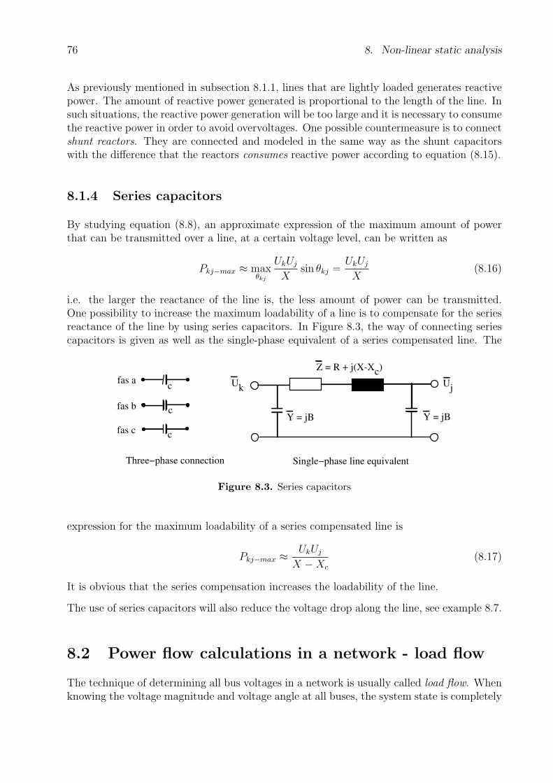
76 8. Non-linear static analysis
As previously mentioned in subsection 8.1.1, lines that are lightly loaded generates reactivepower. The amount of reactive power generated is proportional to the length of the line. Insuch situations, the reactive power generation will be too large and it is necessary to consumethe reactive power in order to avoid overvoltages. One possible countermeasure is to connectshunt reactors. They are connected and modeled in the same way as the shunt capacitorswith the difference that the reactors consumes reactive power according to equation (8.15).
8.1.4 Series capacitors
By studying equation (8.8), an approximate expression of the maximum amount of powerthat can be transmitted over a line, at a certain voltage level, can be written as
Pkj−max ≈ maxθkj
UkUj
Xsin θkj =
UkUj
X(8.16)
i.e. the larger the reactance of the line is, the less amount of power can be transmitted.One possibility to increase the maximum loadability of a line is to compensate for the seriesreactance of the line by using series capacitors. In Figure 8.3, the way of connecting seriescapacitors is given as well as the single-phase equivalent of a series compensated line. The
fas a
fas b
fas c
c
c
c
Three−phase connection Single−phase line equivalent
Uk Uj
Z = R + j(XXc)
Y = jB Y = jB
Figure 8.3. Series capacitors
expression for the maximum loadability of a series compensated line is
Pkj−max ≈ UkUj
X −Xc
(8.17)
It is obvious that the series compensation increases the loadability of the line.
The use of series capacitors will also reduce the voltage drop along the line, see example 8.7.
8.2 Power flow calculations in a network - load flow
The technique of determining all bus voltages in a network is usually called load flow. Whenknowing the voltage magnitude and voltage angle at all buses, the system state is completely

8.2. Power flow calculations in a network - load flow 77
determined and all system properties of interest can be calculated, e.g. line loadings andline losses.
In a network, power can be generated and consumed at many different locations. All locationswhere a line ends is often called bus (or node). In Figure 8.4, the representation of bus k isgiven under the assumption of symmetrical three-phase conditions.
Ik1
Ik2
IkN
~
IGk
IDk
Uk
Figure 8.4. Notation of bus k in a network
The generator generates the current IGk, the load at the bus draws the current IDk and onthe lines to the neighboring buses the currents Ik1, Ik2 . . . IkN flows. According to Kirchoff’sfirst law, the sum of all currents flowing into bus k must equal zero, i.e.
IGk − IDk =N∑
j=1
Ikj (8.18)
By taking the conjugate of equation (8.18) and multiply the equation with the bus voltage,the following holds
UkI∗Gk − UkI
∗Dk =
N∑j=1
UkI∗kj (8.19)
This can be rewritten as an expression for complex power in the per-unit system as
SGk − SDk =N∑
j=1
Skj (8.20)
where
SGk = PGk + jQGk = by the generator generated complex power
SDk = PDk + jQDk = by the load consumed complex power
Skj = Pkj + jQkj = transmitted power to bus j
The power balance at the bus according to equation (8.20) must hold both for the activeand for the reactive part of the expression. By using PGDk and QGDk as notation for the netgeneration of active and reactive power at bus k, respectively, the following expression holds
PGDk = PGk − PDk =N∑
j=1
Pkj (8.21)
QGDk = QGk −QDk =N∑
j=1
Qkj (8.22)

78 8. Non-linear static analysis
i.e. for every bus in the system, the power balance must hold for both active and reactivepower.
Assume that a power system is operating under symmetrical conditions according to Figure8.5. By formulating equation (8.21) and (8.22) at each bus in the system, a system of
~
~
PG1+jQG1
PG2+jQG2
PD2+jQD2
P13+jQ13
P23+jQ23
1
2
3
P31+jQ31
P32+jQ32PD3+jQD3
P12+jQ12
P21+jQ21
U1θ1
U2θ2
U3θ3
Figure 8.5. A three bus power system
equations can be formed as
PG1 = P12 + P13
QG1 = Q12 + Q13
PG2 − PD2 = P21 + P23
QG2 −QD2 = Q21 + Q23
−PD3 = P31 + P32
−QD3 = Q31 + Q32
(8.23)
At each bus in Figure 8.5, four variables are of interest: net generation of active power PGDk,net generation of reactive power QGDk, voltage magnitude Uk and voltage phase angle θk.This gives that the total number of variables for the system are 3 · 4 = 12. The voltagephase angles must be given as an angle in relation to a reference angle. This since the phaseangles are only relative to one another and not absolute. This reduces the number of systemvariables to 12 − 1 = 11. There are only six equations in the system of equations given in8.23, this gives that five quantities must be known to be able to calculate the remainingsix variables. Depending on what quantities that are known at a certain bus, the buses aremainly modeled in three different ways.
PQ-bus, Load bus : For this bus, the net generated power PGDk and QGDk are assumed tobe known. The name PQ-bus is based on that assumption. On the other hand, the voltagemagnitude Uk and the voltage phase angle θk are unknown. A PQ-bus is most often a bus

8.2. Power flow calculations in a network - load flow 79
with a pure load demand, as bus 3 in Figure 8.5. It represents a system bus where the powerconsumption can be considered to be independent of the voltage magnitude. This modelis suitable for a load bus located on the low voltage side of a regulating transformer. Theregulating transformer keeps the load voltage constant independent of the voltage fluctua-tions on the high voltage side of the transformer. Note that a PQ-bus can be a bus withoutgeneration as well as load, i.e. PGDk = QGDk = 0. This holds e.g. at a bus where a line isconnected to a transformer.
PU-bus, Generator bus : In a PU-bus, the net active power generation PGDk as well as thevoltage magnitude Uk are assumed to be known. This gives that the net reactive powergeneration QGDk and the voltage angle θk are unknown. In a PU-bus some sort of voltageregulating device must be connected since the voltage magnitude is independent of the netreactive power generation. For example, in a synchronous machine, the terminal voltage canbe regulated by changing the magnetizing current. In a system, voltage can be regulatedby using controllable components as controllable shunt capacitors and controllable shuntreactors. A standard component is called SVC, Static VAr Compensator. This componentchange the reactive power flow in order to regulate the bus voltage. Assume that bus2 in Figure 8.5 is modeled as a PU-bus. This gives that the active power generation ofthe generator as well as the active power consumption of the load are known. Also thereactive power consumption of the load is known. The bus voltage is constant due to themagnetization system of the generator. The generator may generate or consume reactivepower in such a way that the relation in equation (8.22) holds.
Uθ-nod, Slack bus : At the slack bus (only one bus in each system), the voltage angle ischosen as a reference angle θk, (often 0) and the voltage magnitude is assumed to be known.Unknown quantities are the net generation of both active and reactive power. At this bus,(as for the PU-bus) a voltage regulating component must be present. Since the active poweris allowed to vary, a generator or an active power in-feed into the system is assumed to existat this bus. Since this bus also is the only bus where the active power is allowed to vary,the slack bus will take care of the system losses since they are unknown. If the loads havebeen modeled in the load flow as constant power loads and a line is tripped, the only buswhich will change the active power generation is the slack bus. If bus 1 is chosen as slackbus in Figure 8.5, both PG1 and QG1 are unknown but the voltage U1 is given as well as thereference angle θ1 = 0.
Assume that a system contains N buses and that M of these are PU-buses. A summary ofthe different bus types is given in Table 8.1. As previously mentioned in subsection 8.1.1,
Bus model Number Known quantities Unknown quantitiesUθ-bus, Slack bus 1 U , θ PGD, QGD
PU-bus, Generator bus M PGD, U QGD, θPQ-bus, Load bus N-M-1 PGD, QGD U , θ
Table 8.1. Bus types for load flow calculations
equation (8.6)–(8.7), the active and reactive power transfer on a line can be expressed as afunction of the voltage magnitude and voltage phase angle at both ends of the line. Assumethat the power system in Figure 8.5 is modeled in such a way that bus 1 is a slack bus, bus
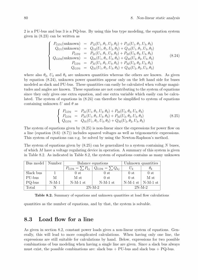
80 8. Non-linear static analysis
2 is a PU-bus and bus 3 is a PQ-bus. By using this bus type modeling, the equation systemgiven in (8.23) can be written as
PGD1(unknown) = P12(U1, θ1, U2, θ2) + P13(U1, θ1, U3, θ3)QG1(unknown) = Q12(U1, θ1, U2, θ2) + Q13(U1, θ1, U3, θ3)
PGD2 = P21(U1, θ1, U2, θ2) + P23(U2, θ2, U3, θ3)QGD2(unknown) = Q21(U1, θ1, U2, θ2) + Q23(U2, θ2, U3, θ3)
PGD3 = P31(U1, θ1, U3, θ3) + P32(U2, θ2, U3, θ3)QGD3 = Q31(U1, θ1, U3, θ3) + Q32(U2, θ2, U3, θ3)
(8.24)
where also θ2, U3 and θ3 are unknown quantities whereas the others are known. As givenby equation (8.24), unknown power quantities appear only on the left hand side for busesmodeled as slack and PU-bus. These quantities can easily be calculated when voltage magni-tudes and angles are known. These equations are not contributing to the system of equationssince they only gives one extra equation, and one extra variable which easily can be calcu-lated. The system of equations in (8.24) can therefore be simplified to system of equationscontaining unknown U and θ as
PGD2 = P21(U1, θ1, U2, θ2) + P23(U2, θ2, U3, θ3)PGD3 = P31(U1, θ1, U3, θ3) + P32(U2, θ2, U3, θ3)QGD3 = Q31(U1, θ1, U3, θ3) + Q32(U2, θ2, U3, θ3)
(8.25)
The system of equations given by (8.25) is non-linear since the expressions for power flow ona line (equation (8.6)–(8.7)) includes squared voltages as well as trigonometric expressions.This system of equations can e.g. be solved by using the Newton-Raphson’s method.
The system of equations given by (8.25) can be generalized to a system containing N buses,of which M have a voltage regulating device in operation. A summary of this system is givenin Table 8.2. As indicated in Table 8.2, the system of equations contains as many unknown
Bus model Number Balance equations Unknown quantitiesPGDk =
∑Pkj QGDk =
∑Qkj Uk θk
Slack bus 1 0 st 0 st 0 st 0 stPU-bus M M st 0 st 0 st M stPQ-bus N-M-1 N-M-1 st N-M-1 st N-M-1 st N-M-1 stTotal N 2N-M-2 2N-M-2
Table 8.2. Summary of equations and unknown quantities at load flow calculations
quantities as the number of equations, and by that, the system is solvable.
8.3 Load flow for a line
As given in section 8.2, constant power loads gives a non-linear system of equations. Gen-erally, this will lead to more complicated calculations. When having only one line, theexpressions are still suitable for calculations by hand. Below, expressions for two possiblecombinations of bus modeling when having a single line are given. Since a slack bus alwaysmust exist, the possible combinations are: slack bus + PU-bus and slack bus + PQ-bus.
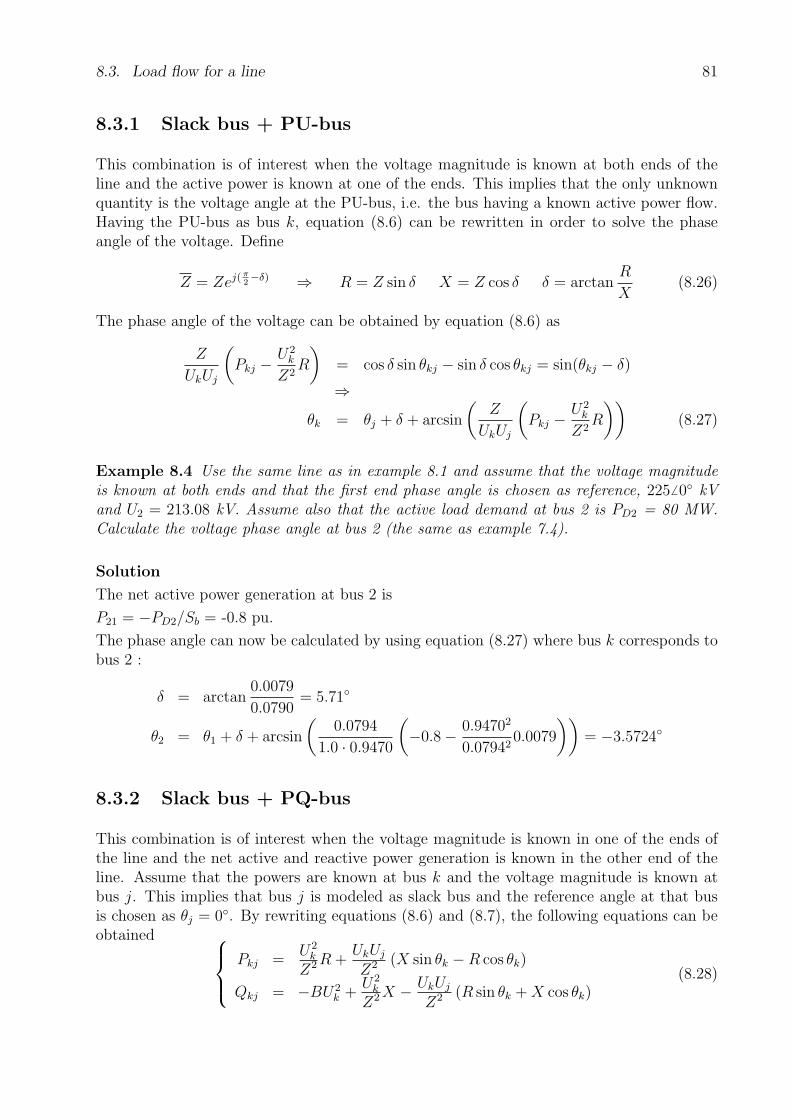
8.3. Load flow for a line 81
8.3.1 Slack bus + PU-bus
This combination is of interest when the voltage magnitude is known at both ends of theline and the active power is known at one of the ends. This implies that the only unknownquantity is the voltage angle at the PU-bus, i.e. the bus having a known active power flow.Having the PU-bus as bus k, equation (8.6) can be rewritten in order to solve the phaseangle of the voltage. Define
Z = Zej(π2−δ) ⇒ R = Z sin δ X = Z cos δ δ = arctan
R
X(8.26)
The phase angle of the voltage can be obtained by equation (8.6) as
Z
UkUj
(Pkj − U2
k
Z2R
)= cos δ sin θkj − sin δ cos θkj = sin(θkj − δ)
⇒θk = θj + δ + arcsin
(Z
UkUj
(Pkj − U2
k
Z2R
))(8.27)
Example 8.4 Use the same line as in example 8.1 and assume that the voltage magnitudeis known at both ends and that the first end phase angle is chosen as reference, 2256 0 kVand U2 = 213.08 kV. Assume also that the active load demand at bus 2 is PD2 = 80 MW.Calculate the voltage phase angle at bus 2 (the same as example 7.4).
Solution
The net active power generation at bus 2 is
P21 = −PD2/Sb = -0.8 pu.
The phase angle can now be calculated by using equation (8.27) where bus k corresponds tobus 2 :
δ = arctan0.0079
0.0790= 5.71
θ2 = θ1 + δ + arcsin
(0.0794
1.0 · 0.9470
(−0.8− 0.94702
0.079420.0079
))= −3.5724
8.3.2 Slack bus + PQ-bus
This combination is of interest when the voltage magnitude is known in one of the ends ofthe line and the net active and reactive power generation is known in the other end of theline. Assume that the powers are known at bus k and the voltage magnitude is known atbus j. This implies that bus j is modeled as slack bus and the reference angle at that busis chosen as θj = 0. By rewriting equations (8.6) and (8.7), the following equations can beobtained
Pkj =U2
k
Z2 R +UkUj
Z2 (X sin θk −R cos θk)
Qkj = −BU2k +
U2k
Z2 X − UkUj
Z2 (R sin θk + X cos θk)(8.28)
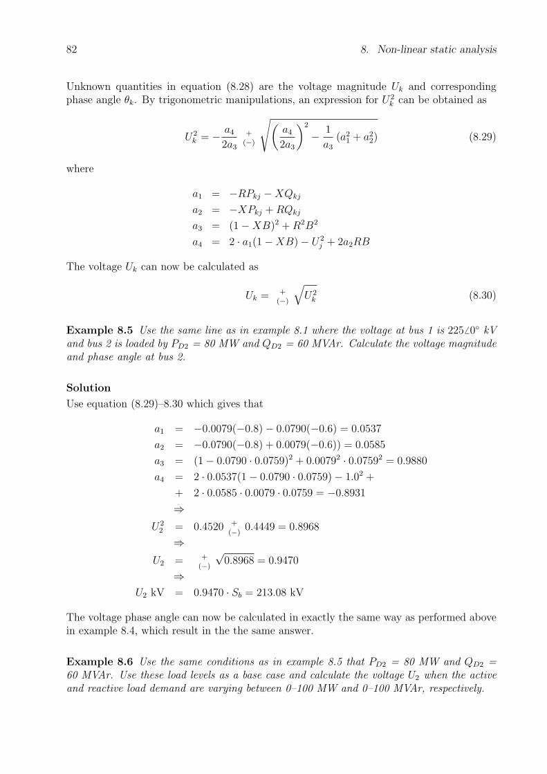
82 8. Non-linear static analysis
Unknown quantities in equation (8.28) are the voltage magnitude Uk and correspondingphase angle θk. By trigonometric manipulations, an expression for U2
k can be obtained as
U2k = − a4
2a3
+
(−)
√(a4
2a3
)2
− 1
a3
(a21 + a2
2) (8.29)
where
a1 = −RPkj −XQkj
a2 = −XPkj + RQkj
a3 = (1−XB)2 + R2B2
a4 = 2 · a1(1−XB)− U2j + 2a2RB
The voltage Uk can now be calculated as
Uk = +
(−)
√U2
k (8.30)
Example 8.5 Use the same line as in example 8.1 where the voltage at bus 1 is 225 6 0 kVand bus 2 is loaded by PD2 = 80 MW and QD2 = 60 MVAr. Calculate the voltage magnitudeand phase angle at bus 2.
Solution
Use equation (8.29)–8.30 which gives that
a1 = −0.0079(−0.8)− 0.0790(−0.6) = 0.0537
a2 = −0.0790(−0.8) + 0.0079(−0.6)) = 0.0585
a3 = (1− 0.0790 · 0.0759)2 + 0.00792 · 0.07592 = 0.9880
a4 = 2 · 0.0537(1− 0.0790 · 0.0759)− 1.02 +
+ 2 · 0.0585 · 0.0079 · 0.0759 = −0.8931
⇒U2
2 = 0.4520 +
(−)0.4449 = 0.8968
⇒U2 = +
(−)
√0.8968 = 0.9470
⇒U2 kV = 0.9470 · Sb = 213.08 kV
The voltage phase angle can now be calculated in exactly the same way as performed abovein example 8.4, which result in the the same answer.
Example 8.6 Use the same conditions as in example 8.5 that PD2 = 80 MW and QD2 =60 MVAr. Use these load levels as a base case and calculate the voltage U2 when the activeand reactive load demand are varying between 0–100 MW and 0–100 MVAr, respectively.
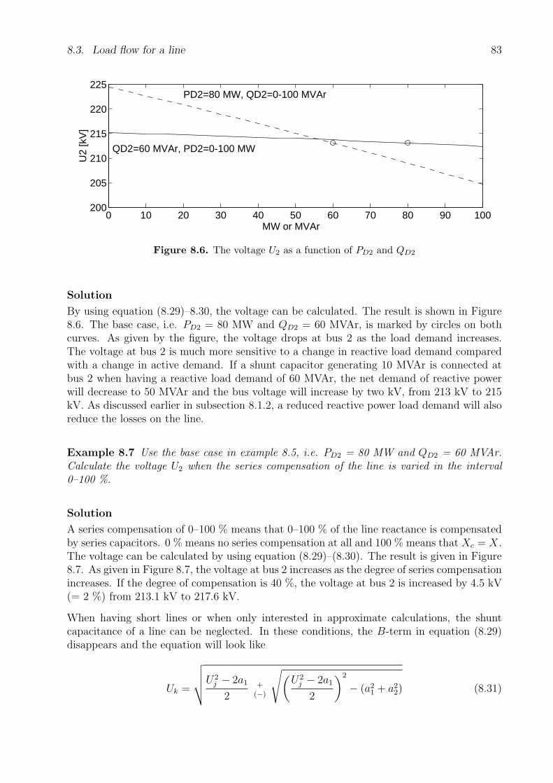
8.3. Load flow for a line 83
0 10 20 30 40 50 60 70 80 90 100200
205
210
215
220
225
QD2=60 MVAr, PD2=0-100 MW
PD2=80 MW, QD2=0-100 MVAr
MW or MVAr
U2
[kV
]
Figure 8.6. The voltage U2 as a function of PD2 and QD2
Solution
By using equation (8.29)–8.30, the voltage can be calculated. The result is shown in Figure8.6. The base case, i.e. PD2 = 80 MW and QD2 = 60 MVAr, is marked by circles on bothcurves. As given by the figure, the voltage drops at bus 2 as the load demand increases.The voltage at bus 2 is much more sensitive to a change in reactive load demand comparedwith a change in active demand. If a shunt capacitor generating 10 MVAr is connected atbus 2 when having a reactive load demand of 60 MVAr, the net demand of reactive powerwill decrease to 50 MVAr and the bus voltage will increase by two kV, from 213 kV to 215kV. As discussed earlier in subsection 8.1.2, a reduced reactive power load demand will alsoreduce the losses on the line.
Example 8.7 Use the base case in example 8.5, i.e. PD2 = 80 MW and QD2 = 60 MVAr.Calculate the voltage U2 when the series compensation of the line is varied in the interval0–100 %.
Solution
A series compensation of 0–100 % means that 0–100 % of the line reactance is compensatedby series capacitors. 0 % means no series compensation at all and 100 % means that Xc = X.The voltage can be calculated by using equation (8.29)–(8.30). The result is given in Figure8.7. As given in Figure 8.7, the voltage at bus 2 increases as the degree of series compensationincreases. If the degree of compensation is 40 %, the voltage at bus 2 is increased by 4.5 kV(= 2 %) from 213.1 kV to 217.6 kV.
When having short lines or when only interested in approximate calculations, the shuntcapacitance of a line can be neglected. In these conditions, the B-term in equation (8.29)disappears and the equation will look like
Uk =
√√√√U2j − 2a1
2+
(−)
√(U2
j − 2a1
2
)2
− (a21 + a2
2) (8.31)
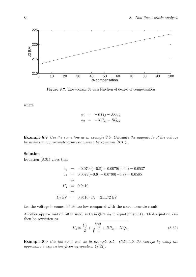
84 8. Non-linear static analysis
0 10 20 30 40 50 60 70 80 90 100210
215
220
225
% compensation
U2
[kV
]
Figure 8.7. The voltage U2 as a function of degree of compensation
where
a1 = −RPkj −XQkj
a2 = −XPkj + RQkj
Example 8.8 Use the same line as in example 8.5. Calculate the magnitude of the voltageby using the approximate expression given by equation (8.31).
Solution
Equation (8.31) gives that
a1 = −0.0790(−0.8) + 0.0079(−0.6) = 0.0537
a2 = 0.0079(−0.6)− 0.0790(−0.8) = 0.0585
⇒U2 = 0.9410
⇒U2 kV = 0.9410 · Sb = 211.72 kV
i.e. the voltage becomes 0.6 % too low compared with the more accurate result.
Another approximation often used, is to neglect a2 in equation (8.31). That equation canthen be rewritten as
Uk ≈ Uj
2+
√U2
j
4+ RPkj + XQkj (8.32)
Example 8.9 Use the same line as in example 8.5. Calculate the voltage by using theapproximate expression given by equation (8.32).
8.4. Newton-Raphson method 85
Solution
Equation (8.32) gives that
U2 = 0.9430
⇒U2(kV ) = 0.9439 · Sb = 212.18 kV
i.e. the calculated voltage is 0.4 % too low. As indicated in this example, equation (8.32)gives a good approximation of the voltage drop on the line. In the equation, it is also clearlygiven that the active and reactive load demand have influence on the voltage drop. Thereason why the voltage drop is more sensitive to a change in reactive power compared witha change in active power, is that the line reactance dominates the line resistance.
8.4 Newton-Raphson method
8.4.1 Theory
The Newton-Raphson method may be applied to solve for x1, x2, · · · , xn of the followingnon-linear equations,
g1(x1, x2, · · · , xn) = f1(x1, x2, · · · , xn)− b1 = 0
g2(x1, x2, · · · , xn) = f2(x1, x2, · · · , xn)− b2 = 0
...
gn(x1, x2, · · · , xn) = fn(x1, x2, · · · , xn)− bn = 0
(8.33)
or in the vector formg(x) = f(x)− b = 0 (8.34)
where
x =
x1
x2...
xn
, g(x) =
g1(x)g2(x)
...gn(x)
, f(x) =
f1(x)f2(x)
...fn(x)
, b =
b1
b2...bn
x is an n× 1 vector which contains variables, b is an n× 1 vector which contains constants,and f(x) is an n× 1 vector-valued function.
Taylor’s series expansion of (8.34) is the basis for the Newton-Raphson method of solving(8.34) in an iterative manner. From an initial estimate (or guess) x(0), a sequence of graduallybetter estimates x(1), x(2), x(3), · · · will be made that hopefully will converge to the solutionx∗.
Let x∗ be the solution of (8.34), i.e. g(x∗) = 0, and x(i) be an estimate of x∗. Let also∆x(i) = x∗ − x(i). Equation (8.34) can now be written as
g(x∗) = g(x(i) + ∆x(i)) = 0 (8.35)
86 8. Non-linear static analysis
Taylor’s series expansion of (8.35) gives
g(x(i) + ∆x(i)) = g(x(i)) + JAC(x(i))∆x(i) = 0 (8.36)
where
JAC(x(i)) =
[∂g(x)
∂x
]
x=x(i)
=
∂g1(x)∂x1
· · · ∂g1(x)∂xn
.... . .
...∂gn(x)
∂x1· · · ∂gn(x)
∂xn
x=x(i)
(8.37)
where, JAC ia called the jacobian of g.
From (8.36), ∆x(i) can be calculated as follows
JAC(x(i))∆x(i) = 0− g(x(i)) = ∆g(x(i)) ⇒ (8.38)
∆x(i) =[JAC(x(i))
]−1
∆g(x(i)) (8.39)
Since g(x(i)) = f(x(i))− b, ∆g(x(i)) is given by
∆g(x(i)) = b− f(x(i)) = −g(x(i)) (8.40)
Furthermore, since b is constant, JAC(x(i)) is given by
JAC(x(i)) =
[∂g(x)
∂x
]
x=x(i)
=
[∂f(x)
∂x
]
x=x(i)
=
∂f1(x)∂x1
· · · ∂f1(x)∂xn
.... . .
...∂fn(x)
∂x1· · · ∂fn(x)
∂xn
x=x(i)
(8.41)
Therefore, ∆x(i) can be calculated as follows
∆x(i) =
∆x(i)1
...
∆x(i)n
=
∂f1(x)∂x1
· · · ∂f1(x)∂xn
.... . .
...∂fn(x)
∂x1· · · ∂fn(x)
∂xn
−1
x=x(i)
b1 − f1(x(i)1 , · · · , x
(i)n )
...
bn − fn(x(i)1 , · · · , x
(i)n )
(8.42)
Finally, the following is obtained
i = i + 1
x(i) = x(i−1) + ∆x(i−1)
The intention is that x(1) will estimate the solution x∗ better than what x(0) does. In thesame manner, x(2), x(3) , · · · can be determined until a specified condition is satisfied. Thus,we obtain an iterative method according to the flowchart in Figure 8.8.
Example 8.10 Using the Newton-Raphson method, solve for x of the equation
g(x) = k1 x + k2 cos(x− k3)− k4 = 0
Let k1 = −0.2, k2 = 1.2, k3 = −0.07, k4 = 0.4 and ε = 10−4. (This equation is used in theassignment D1.)
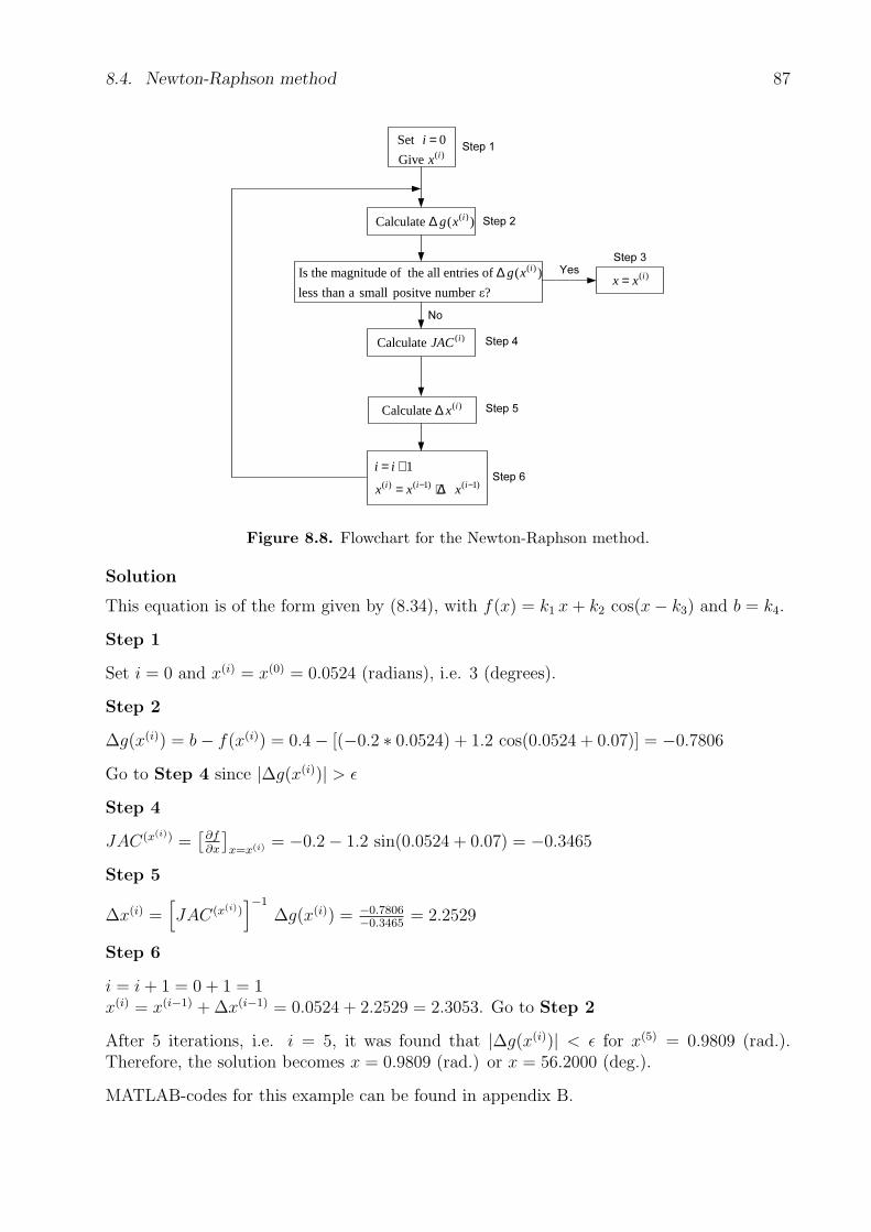
8.4. Newton-Raphson method 87
Yes
No
( )Give ix
Set 0i =
( )ix x=
Step 1
Step 2
Step 3
( )Calculate ( )ig x∆
( )Is the magnitude of the all entries of ( )
less than a small positve number ε?
ig x∆
( ) ( 1) ( 1)
1i i i
i i
x x x− −
= +
= + ∆
Step 4
Step 5( )Calculate ix∆
Step 6
( )Calculate iJAC
Figure 8.8. Flowchart for the Newton-Raphson method.
Solution
This equation is of the form given by (8.34), with f(x) = k1 x + k2 cos(x− k3) and b = k4.
Step 1
Set i = 0 and x(i) = x(0) = 0.0524 (radians), i.e. 3 (degrees).
Step 2
∆g(x(i)) = b− f(x(i)) = 0.4− [(−0.2 ∗ 0.0524) + 1.2 cos(0.0524 + 0.07)] = −0.7806
Go to Step 4 since |∆g(x(i))| > ε
Step 4
JAC(x(i)) =[
∂f∂x
]x=x(i) = −0.2− 1.2 sin(0.0524 + 0.07) = −0.3465
Step 5
∆x(i) =[JAC(x(i))
]−1
∆g(x(i)) = −0.7806−0.3465
= 2.2529
Step 6
i = i + 1 = 0 + 1 = 1x(i) = x(i−1) + ∆x(i−1) = 0.0524 + 2.2529 = 2.3053. Go to Step 2
After 5 iterations, i.e. i = 5, it was found that |∆g(x(i))| < ε for x(5) = 0.9809 (rad.).Therefore, the solution becomes x = 0.9809 (rad.) or x = 56.2000 (deg.).
MATLAB-codes for this example can be found in appendix B.

88 8. Non-linear static analysis
Analysis of Example 8.10
Figure 8.9 shows variations of g(x) versus x. The figure shows that the system (or equation)has only three solutions, i.e. the points at which g(x) = 0. Due to practical issues, x∗
indicted with (O) in the figure is the interesting solution.
−400 −300 −200 −100 0 100 200 300 400−2.5
−2
−1.5
−1
−0.5
0
0.5
1
1.5
2
2.5
x
g(x
)
x*
Figure 8.9. Variations of g(x) vs. x.
Figure 8.10 shows how the equation is solved by the Newton-Raphson method.
We first guess the initial estimate x(0). In this case x(0) = 0.0524 (rad.), i.e 3 (deg.). The
tangent to g(x) through the point(x(0) , g(x(0))
), i.e. g′(x(0)) =
[dg(x)
dx
]x=x(0)
= JAC(x(0)),
intersects the x–axis at point x(1). The equation for this tangent is given by
Y − g(x(0)) = g′(x(0)) ∗ (x− x(0))
The intersection point x(1) is obtained by setting Y = 0, i.e.
x(1) = x(0) − g(x(0))
g′(x(0))= x(0) − (
g′(x(0)))−1
g(x(0))
∆x(1) = x(1) − x(0) = − (g′(x(0))
)−1g(x(0)) =
[JAC(x(0))
]−1
∆g(x(0))
In a similar manner, x(2) can be obtained which is hopefully a better estimate than x(1). Asshown in the figure, from x(2) we obtain x(3) which is a better estimate of x∗ than what x(2)
does. This iterative method will be continued until |∆g(x)| < ε.
Example 8.11 Solve for x in Example 8.10, but let x(0) = 0.0174 (rad.), i.e. 1 (deg.).
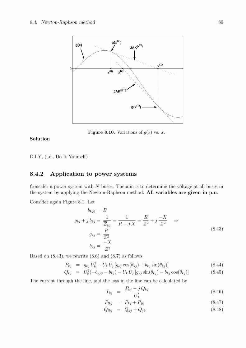
8.4. Newton-Raphson method 89
0
g(x)
x(0)
x(1)
x(2)
g(x(0))
JAK(x(0)
)
g(x(1))
JAK(x(1)
)
Figure 8.10. Variations of g(x) vs. x.Solution
D.I.Y, (i.e., Do It Yourself)
8.4.2 Application to power systems
Consider a power system with N buses. The aim is to determine the voltage at all buses inthe system by applying the Newton-Raphson method. All variables are given in p.u.
Consider again Figure 8.1. Let
bkj0 = B
gkj + j bkj =1
Zkj
=1
R + j X=
R
Z2+ j
−X
Z2⇒
gkj =R
Z2
bkj =−X
Z2
(8.43)
Based on (8.43), we rewrite (8.6) and (8.7) as follows
Pkj = gkj U2k − Uk Uj [gkj cos(θkj) + bkj sin(θkj)] (8.44)
Qkj = U2k (−bkj0 − bkj)− Uk Uj [gkj sin(θkj)− bkj cos(θkj)] (8.45)
The current through the line, and the loss in the line can be calculated by
Ikj =Pkj − j Qkj
U∗k
(8.46)
Plkj = Pkj + Pjk (8.47)
Qlkj = Qkj + Qjk (8.48)

90 8. Non-linear static analysis
Consider again Figure 8.4. Let Y = G+ jB denote the admittance matrix of the system (orY-matrix), where Y is an N ×N matrix, i.e. the system has N buses. The relation betweenthe injected currents into the buses and the voltages at the buses is given by I = Y U , seesection 5.1. Therefore, the injected current into bus k is given by Ik =
∑Nj=1 Y kj U j.
The injected complex power into bus k can now be calculated by
Sk = Uk I∗k = Uk
N∑j=1
Y∗kjU
∗j = Uk
N∑j=1
(Gkj − jBkj) Uj(cos(θkj) + j sin(θkj))
=
(Uk
N∑j=1
Uj [Gkj cos(θkj) + Bkj sin(θkj)]
)+ j
(Uk
N∑j=1
Uj [Gkj sin(θkj)−Bkj cos(θkj)]
)
Let Pk denote the real part of Sk, i.e. the injected active power, and Qk denote the imaginarypart of Sk, i.e. the injected reactive power, as follows:
Pk = Uk
N∑j=1
Uj [Gkj cos(θkj) + Bkj sin(θkj)]
Qk = Uk
N∑j=1
Uj [Gkj sin(θkj)−Bkj cos(θkj)]
(8.49)
Note that Gkj = −gkj and Bkj = −bkj for k 6= j. Furthermore,
Pk =N∑
j=1
Pkj
Qk =N∑
j=1
Qkj
Equations (8.21) and (8.22) can now be rewritten as
Pk − PGDk = 0
Qk −QGDk = 0(8.50)
which are of the form given in equation (8.34), where
x =
θ
U
=
θ1...
θN
U1...
UN
, f(θ, U) =
fP (θ, U)
fQ(θ, U)
=
P1...
PN
Q1...
QN
, b =
bP
bQ
=
PGD1...
PGDN
QGD1...
QGDN
(8.51)
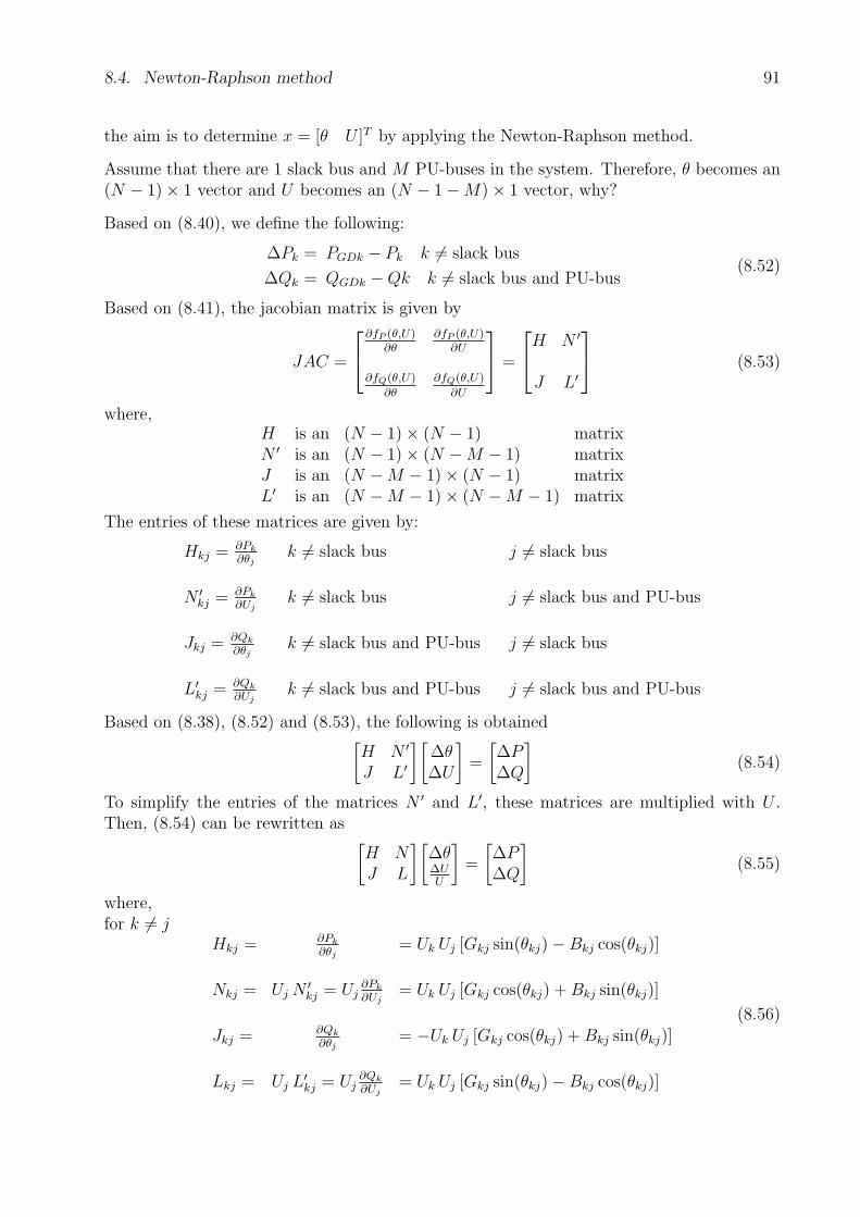
8.4. Newton-Raphson method 91
the aim is to determine x = [θ U ]T by applying the Newton-Raphson method.
Assume that there are 1 slack bus and M PU-buses in the system. Therefore, θ becomes an(N − 1)× 1 vector and U becomes an (N − 1−M)× 1 vector, why?
Based on (8.40), we define the following:
∆Pk = PGDk − Pk k 6= slack bus
∆Qk = QGDk −Qk k 6= slack bus and PU-bus(8.52)
Based on (8.41), the jacobian matrix is given by
JAC =
∂fP (θ,U)∂θ
∂fP (θ,U)∂U
∂fQ(θ,U)
∂θ
∂fQ(θ,U)
∂U
=
H N ′
J L′
(8.53)
where,H is an (N − 1)× (N − 1) matrixN ′ is an (N − 1)× (N −M − 1) matrixJ is an (N −M − 1)× (N − 1) matrixL′ is an (N −M − 1)× (N −M − 1) matrix
The entries of these matrices are given by:
Hkj = ∂Pk
∂θjk 6= slack bus j 6= slack bus
N ′kj = ∂Pk
∂Ujk 6= slack bus j 6= slack bus and PU-bus
Jkj = ∂Qk
∂θjk 6= slack bus and PU-bus j 6= slack bus
L′kj = ∂Qk
∂Ujk 6= slack bus and PU-bus j 6= slack bus and PU-bus
Based on (8.38), (8.52) and (8.53), the following is obtained[H N ′
J L′
][∆θ∆U
]=
[∆P∆Q
](8.54)
To simplify the entries of the matrices N ′ and L′, these matrices are multiplied with U .Then, (8.54) can be rewritten as
[H NJ L
][∆θ∆UU
]=
[∆P∆Q
](8.55)
where,for k 6= j
Hkj = ∂Pk
∂θj= Uk Uj [Gkj sin(θkj)−Bkj cos(θkj)]
Nkj = Uj N ′kj = Uj
∂Pk
∂Uj= Uk Uj [Gkj cos(θkj) + Bkj sin(θkj)]
Jkj = ∂Qk
∂θj= −Uk Uj [Gkj cos(θkj) + Bkj sin(θkj)]
Lkj = Uj L′kj = Uj∂Qk
∂Uj= Uk Uj [Gkj sin(θkj)−Bkj cos(θkj)]
(8.56)
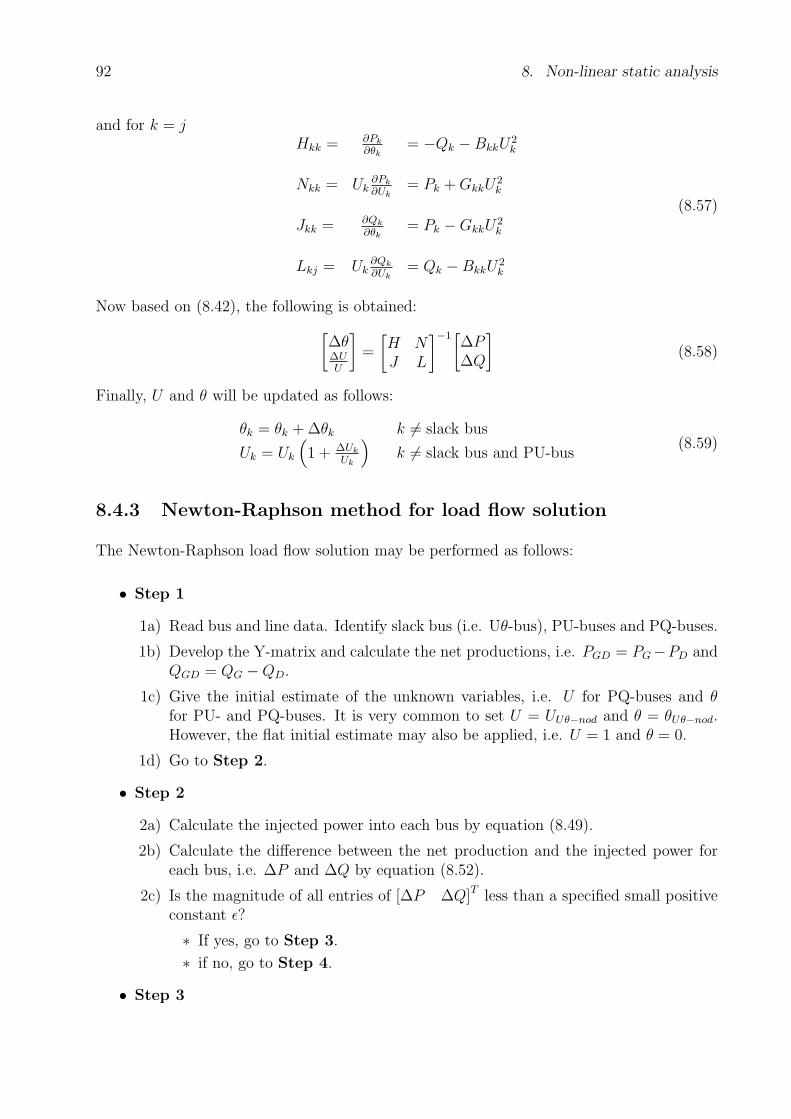
92 8. Non-linear static analysis
and for k = jHkk = ∂Pk
∂θk= −Qk −BkkU
2k
Nkk = Uk∂Pk
∂Uk= Pk + GkkU
2k
Jkk = ∂Qk
∂θk= Pk −GkkU
2k
Lkj = Uk∂Qk
∂Uk= Qk −BkkU
2k
(8.57)
Now based on (8.42), the following is obtained:
[∆θ∆UU
]=
[H NJ L
]−1[∆P∆Q
](8.58)
Finally, U and θ will be updated as follows:
θk = θk + ∆θk k 6= slack bus
Uk = Uk
(1 + ∆Uk
Uk
)k 6= slack bus and PU-bus
(8.59)
8.4.3 Newton-Raphson method for load flow solution
The Newton-Raphson load flow solution may be performed as follows:
• Step 1
1a) Read bus and line data. Identify slack bus (i.e. Uθ-bus), PU-buses and PQ-buses.
1b) Develop the Y-matrix and calculate the net productions, i.e. PGD = PG−PD andQGD = QG −QD.
1c) Give the initial estimate of the unknown variables, i.e. U for PQ-buses and θfor PU- and PQ-buses. It is very common to set U = UUθ−nod and θ = θUθ−nod.However, the flat initial estimate may also be applied, i.e. U = 1 and θ = 0.
1d) Go to Step 2.
• Step 2
2a) Calculate the injected power into each bus by equation (8.49).
2b) Calculate the difference between the net production and the injected power foreach bus, i.e. ∆P and ∆Q by equation (8.52).
2c) Is the magnitude of all entries of [∆P ∆Q]T less than a specified small positiveconstant ε?
∗ If yes, go to Step 3.
∗ if no, go to Step 4.
• Step 3

8.4. Newton-Raphson method 93
3a) Calculate the power flows by equations (8.44) and (8.45).
3b) Calculate the generated powers, i.e. PG and QG in the slack bus, and QG in thePU-buses by equation (8.50).
3c) Print out the results.
• Step 4
4a) Calculate the jacobian by equations (8.56) and (8.57).
4b) Go to Step 5.
• Step 5
5a) Calculate[∆θ ∆U
U
]Tby equation (8.58).
5b) Go to Step 6.
• Step 6
6a) Update U and θ by equation (8.59).
6b) Go till Step 2.
Example 8.12 Consider the power system shown in Figure 8.5. The following data (all inp.u.) are known:
• Line between Bus 1 and Bus 2: short line, Z12 = j 0.2
• Line between Bus 1 and Bus 3: short line, Z13 = j 0.4
• Line between Bus 2 and Bus 2: short line, Z23 = j 0.5
• Bus 1: U1 = 1, θ1 = 0
• Bus 2: U2 = 1, PG2 = 2, PD2 = 1, QD2 = 0.2
• Bus 3: PD3 = 2, QD3 = −0.4
By applying the Newton-Raphson method, calculate PG1, QG1 and QG2 after 4 iterations.
Solution
Step 11a)y12 = 1
Z12= −j 5 , y13 = 1
Z13= −j 2.5 , y23 = 1
Z23= −j 2
Bus 1= slack bus , Bus 2= PU-bus , Bus 3= PQ-bus

94 8. Non-linear static analysis
1b)y11 = y12 + y13 , y22 = y12 + y23 , y33 = y13 + y23
Y =
y11 −y12 −y13
−y12 y22 −y23
−y13 −y23 y33
=
jB11 jB12 jB13
jB21 jB22 jB23
jB31 jB32 jB33
=
−j 7.5 j 5 j 2.5
j 5 −j 7 j 2j 2.5 j 2 −j 4.5
= jB
Note that Y = G + jB. However, since the lines are lossless, i.e. Rline = 0, we have G = 0.
PGD2 = PG2 − PD2 = 2− 1 = 1PGD3 = PG3 − PD3 = 0− 2 = −2QGD3 = QG3 −QD3 = 0− (−0.4) = 0.4
1c)U3 = 1 , θ2 = 0 , θ3 = 0
Iteration 1
Step 22a)
P1 = U1 [U2B12 sin(θ1 − θ2) + U3B13 sin(θ1 − θ3)] =
= 1 ∗ [1 ∗ 5 ∗ sin(0− 0) + 1 ∗ 2.5 ∗ sin(0− 0)] = 0
P2 = U2 [U1B21 sin(θ2 − θ1) + U3B23 sin(θ2 − θ3)] =
= 1 ∗ [1 ∗ 5 ∗ sin(0− 0) + 1 ∗ 2 ∗ sin(0− 0)] = 0
P3 = U3 [U1B31 sin(θ3 − θ1) + U2B32 sin(θ3 − θ2)] =
= 1 ∗ [1 ∗ 2.5 ∗ sin(0− 0) + 1 ∗ 2 ∗ sin(0− 0)] = 0
Q1 = −U1 [U2B12 cos(θ1 − θ2) + U3B13 cos(θ1 − θ3) + U1B11] =
= −1 ∗ [1 ∗ 5 ∗ cos(0− 0) + 1 ∗ 2.5 ∗ cos(0− 0) + 1 ∗ (−7.5)] = 0
Q2 = −U2 [U1B21 cos(θ2 − θ1) + U3B23 cos(θ2 − θ3) + U2B22] =
= −1 ∗ [1 ∗ 5 ∗ cos(0− 0) + 1 ∗ 2 ∗ cos(0− 0) + 1 ∗ (−7)] = 0
Q3 = −U3 [U1B31 cos(θ3 − θ1) + U2B32 cos(θ3 − θ2) + U3B33] =
= −1 ∗ [1 ∗ 2.5 ∗ cos(0− 0) + 1 ∗ 2 ∗ cos(0− 0) + 1 ∗ (−4.5)] = 0
2b)
∆P =
[∆P2
∆P3
]=
[PGD2 − P2
PGD3 − P3
]=
[1− 0−2− 0
]=
[1−2
]
∆Q =[∆Q3
]=
[QGD3 −Q3
]=
[0.4− 0
]=
[0.4
]
2c)Go directly to Step 4
Step 44a)
H =
∂P2
∂θ2
∂P2
∂θ3
∂P3
∂θ2
∂P3
∂θ3
, N =
U3∂P2
∂U3
U3∂P3
∂U3
, L =
[∂Q3
∂θ2
∂Q3
∂θ3
], J =
[U3
∂Q3
∂U3
]

8.4. Newton-Raphson method 95
JAC =
H N
L J
=
∂P2
∂θ2
∂P2
∂θ3U3
∂P2
∂U3
∂P3
∂θ2
∂P3
∂θ3U3
∂P3
∂U3
∂Q3
∂θ2
∂Q3
∂θ3U3
∂Q3
∂U3
where,
H:
∂P2
∂θ2
= −Q2 −B22U22 = −0− (−7 ∗ 12) = 7
∂P2
∂θ3
= −U2U3B23 cos(θ2 − θ3) = −1 ∗ 1 ∗ 2 ∗ cos(0− 0) = −2
∂P3
∂θ2
= −U3U2B32 cos(θ3 − θ2) = −1 ∗ 1 ∗ 2 ∗ cos(0− 0) = −2
∂P3
∂θ3
= −Q3 −B33U23 = −0− (−4.5 ∗ 12) = 4.5
N:
U3∂P2
∂U3
= U2U3B23 sin(θ2 − θ3) = 1 ∗ 1 ∗ 2 ∗ sin(0− 0) = 0
U3∂P3
∂U3
= P3 = 0
J:
∂Q3
∂θ2
= −U3U2B32 sin(θ3 − θ2) = −1 ∗ 1 ∗ 2 ∗ sin(0− 0) = 0
∂Q3
∂θ3
= P3 = 0
L:
U3∂Q3
∂U3
= Q3 −B33U23 = 0− (−4.5 ∗ 12) = 4.5
Step 55a)
∆θ2
∆θ3
∆U3
U3
=
∂P2
∂θ2
∂P2
∂θ3U3
∂P2
∂U3
∂P3
∂θ2
∂P3
∂θ3U3
∂P3
∂U3
∂Q3
∂θ2
∂Q3
∂θ3U3
∂Q3
∂U3
−1
∆P2
∆P3
∆Q3
=
7 −2 0
−2 4.5 0
0 0 4.5
−1
1
−2
0.4
=
0.0182
−0.4364
0.0889

96 8. Non-linear static analysis
Step 66a)θ2 = θ2 + ∆θ2 = 0 + 0.0182 = 0.0182
θ3 = θ3 + ∆θ3 = 0 + (−0.4364) = −0.4364
U3 = U3(1 + ∆U3
U3) = 1 ∗ (1 + 0.0889) = 1.0889
6b)Go to step 2
Iteration 2Step 22a)
P1 = 1 ∗ [1 ∗ 5 ∗ sin(0− 0.0182) + 1.0889 ∗ 2.5 ∗ sin(0 + 0.4364)] = 1.0596
P2 = 1 ∗ [1 ∗ 5 ∗ sin(0.0182− 0) + 1.0889 ∗ 2 ∗ sin(0.0182 + 0.4364)] = 1.0471
P3 = 1.0889 ∗ [1 ∗ 2.5 ∗ sin(−0.4364− 0) + 1 ∗ 2 ∗ sin(−0.4364− 0.0182)] = −2.1067
Q1 = −1 ∗ [1 ∗ 5 ∗ cos(0− 0.0182) + 1.0889 ∗ 2.5 ∗ cos(0 + 0.4364) + 1 ∗ (−7.5)] = 0.0337
Q2 = −1 ∗ [1 ∗ 5 ∗ cos(0.0182− 0) + 1.0889 ∗ 2 ∗ cos(0.0182 + 0.4364) + 1 ∗ (−7)] = 0.0442
Q3 = −1.0889 ∗ [1 ∗ 2.5 ∗ cos(−0.4364− 0) + 1 ∗ 2 ∗ cos(−0.4364− 0.0182) + 1.0889 ∗ (−4.5)]
= 0.9118
2b)
∆P =
[∆P2
∆P3
]=
[PGD2 − P2
PGD3 − P3
]=
[1− 1.0471−2 + 2.1067
]=
[−0.04710.1067
]
∆Q =[∆Q3
]=
[QGD3 −Q3
]=
[0.4− 0.9118
]=
[−0.5118]
2c)Go to Step 4
Step 44a)H:
∂P2
∂θ2
= −Q2 −B22U22 = −0.0442− (−7 ∗ 12) = 6.9558
∂P2
∂θ3
= −U2U3B23 cos(θ2 − θ3) = −1 ∗ 1.0889 ∗ 2 ∗ cos(0.0182 + 0.4364) = −1.9566
∂P3
∂θ2
= −U3U2B32 cos(θ3 − θ2) = −1.0889 ∗ 1 ∗ 2 ∗ cos(−0.0182− 0.4364) = −1.9566
∂P3
∂θ3
= −Q3 −B33U23 = −0.9118− (−4.5 ∗ 1.08892) = 4.4238

8.4. Newton-Raphson method 97
N:
U3∂P2
∂U3
= U2U3B23 sin(θ2 − θ3) = 1 ∗ 1.0889 ∗ 2 ∗ sin(0.0182 + 0.4364) = 0.9562
U3∂P3
∂U3
= P3 = −2.1067
J:∂Q3
∂θ2
= −U3U2B32 sin(θ3 − θ2) = −1.0889 ∗ 1 ∗ 2 ∗ sin(−0.0182− 0.4364) = 0.9562
∂Q3
∂θ3
= P3 = −2.1067
L:
U3∂Q3
∂U3
= Q3 −B33U23 = 0.9118− (−4.5 ∗ 1.08892) = 6.2473
Step 55a)
∆θ2
∆θ3
∆U3
U3
=
6.9558 −1.9566 0.9562
−1.9566 4.4238 −2.1067
0.9562 −2.1067 6.2473
−1
−0.0471
0.1067
−0.5118
=
0.0004
−0.0175
−0.0879
Step 66a)θ2 = θ2 + ∆θ2 = 0.0182 + 0.0004 = 0.0186
θ3 = θ3 + ∆θ3 = −0.4364− 0.0175 = −0.4539
U3 = U3(1 + ∆U3
U3) = 1.0889 ∗ (1− 0.0879) = 0.9932
6b)Go to step 2
Iteration 3
With these new values (in step 6) for θ2, θ3 and U3, we run the third iteration which givesthese updated values, i.e. θ2 = 0.0186, θ3 = −0.4611 and U3 = 0.9824. Next we run theforth iteration with these updated values as follows:
Step 2 → Step 4 → Step 5
5a)
∆θ2
∆θ3
∆U3
U3
= · · · =
0
−0.0002
−0.0002

98 8. Non-linear static analysis
Step 6
6a)θ2 = θ2 + ∆θ2 = 0.0186 + 0 = 0.0186
θ3 = θ3 + ∆θ3 = −0.4611− 0.0002 = −0.4613
U3 = U3 + (1 + ∆U3
U3) = 0.9824(1− 0.0002) = 0.9822
Now go to step 3
Step 3
3b)
P1 = U1 [U2B12 sin(θ1 − θ2) + U3B13 sin(θ1 − θ3)] =
= 1 ∗ [1 ∗ 5 ∗ sin(0− 0.0186) + 0.9822 ∗ 2.5 ∗ sin(0 + 0.4613)] = 1.0000
Q1 = −U1 [U2B12 cos(θ1 − θ2) + U3B13 cos(θ1 − θ3) + U1B11] =
= −1 ∗ [1 ∗ 5 ∗ cos(0− 0.0186) + 0.9822 ∗ 2.5 ∗ cos(0 + 0.4613) + 1 ∗ (−7.5)] = 0.3020
Q2 = −U2 [U1B21 cos(θ2 − θ1) + U3B23 cos(θ2 − θ3) + U2B22] =
= −1 ∗ [1 ∗ 5 ∗ cos(0.0186− 0) + 0.9822 ∗ 2 ∗ cos(0.0186 + 0.4613) + 1 ∗ (−7)] = 0.2583
PG1 = P1 + PD1 = 1 + 0 = 1
QG1 = Q1 + QD1 = 0.3020 + 0 = 0.3020
QG2 = Q2 + QD2 = 0.2583 + 0.2 = 0.4583
Matlab-codes for this example can be found in appendix C.
Chapter 9
Analysis of three-phase systems using lineartransformations
In this chapter, the possibilities of using linear transformations in order to simplify the anal-ysis of three-phase systems, are briefly discussed. These transformations are general and arevalid under both symmetrical and un-symmetrical conditions. By generalizing the expres-sions for a symmetric three-phase voltage given in equations (3.11) and (3.15), correspondingexpressions for an arbitrary three-phase voltage at constant frequency can be obtained as
ua(t) = UMa cos(ωt + γa)ub(t) = UMb cos(ωt + γb)uc(t) = UMc cos(ωt + γc)
Ua = Ua 6 γaU b = Ub 6 γbU c = Uc 6 γc
(9.1)
where UMa, UMb, UMc are peak values, Ua, Ub, Uc are RMS-values and γa, γb, γc are phaseangles of the three voltages. For the un-symmetrical currents, corresponding expressionshold as
ia(t) = IMa cos(ωt + γa − φa)ib(t) = IMb cos(ωt + γb − φb)ic(t) = IMc cos(ωt + γc − φc)
Ia = Ia 6 γa − φa
Ib = Ib 6 γb − φb
Ic = Ic 6 γc − φc
(9.2)
where IMa, IMb, IMc are peak values, Ia, Ib, Ic are RMS-values of the three phase currentswhereas φa, φb, φc are the phase of the currents in relation to the corresponding phasevoltage.
The mean value of the total three-phase active power can be calculated as
P3 =UMa√
2
IMa√2
cos φa +UMb√
2
IMb√2
cos φb +UMc√
2
IMc√2
cos φc (9.3)
whereas the total three-phase complex power is
S3 = UaI∗a + U bI
∗b + U cI
∗c = (UaIa cos φa + UbIb cos φb + UcIc cos φc) +
+ j(UaIa sin φa + UbIb sin φb + UcIc sin φc) (9.4)
This phase representation is in many cases sufficient for a three-phase system analysis. Thereare a number of important cases when the analysis can greatly be simplified by using lineartransformations.
This chapter discuss the following items. First, the advantages of using linear transfor-mations in three-phase system analysis are generally discussed. Later on, some specifictransformations to be used in certain conditions are given. In order to really understandthe subject of transformations, the reader is referred to text books on the subject, e.g. inelectric machine theory or high power electronics. In chapter 10, one of the transformationsof interest, symmetrical components, is discussed in more detail. The purpose of chapter 9is to show that the idea and the mathematics behind the transformations are the same. Itis only the choice of linear transformation, i.e. transformation matrix, that is different.
99

100 9. Analysis of three-phase systems using linear transformations
9.1 Linear transformations
By using transformations, components are mapped from an original space (the original spaceis here the instantaneous values or the complex representation of the phase quantities) to animage space. A linear transformation means that the components in the image space are alinear combination of the original space. The complex values of the phase voltages can bemapped with a linear transformation as
UA = waaUa + wabU b + wacU c
UB = wbaUa + wbbU b + wbcU c (9.5)
UC = wcaUa + wcbU b + wccU c
which in matrix form can be written as
UA
UB
UC
=
waa wab wac
wba wbb wbc
wca wcb wcc
Ua
U b
U c
(9.6)
or in a more compact notationUABC = WUabc (9.7)
The elements in matrix W are independent of the values of the original and image spacecomponents. In this example, the components in the original space Ua, U b and U c aremapped by using the linear transformation W to the image space components UA, UB andUC . The original space components can be calculated from the image space components byusing the inverse of matrix W (W−1 = T), i.e.
Uabc = W−1UABC = TUABC (9.8)
The only mappings that are of interest, are those where W−1 are existing. In the following,the matrix T or its inverse T−1 will represent the linear transformation.
9.1.1 Power invarians
A usual demand for the linear transformations in power system analysis is that it should bepossible to calculate the electric power in the image space by using the same expressions asin the original space and that the two spaces should give the same result. A transformationthat can meet that requirement is called power invariant. Using the complex representation,the electric power in the original space can be calculated by using equation (9.4), this gives
Sabc = UaI∗a + U bI
∗b + U cI
∗c = UT
abcI∗abc (9.9)
and in the image space, the corresponding expression is
SABC = UAI∗A + UBI
∗B + UCI
∗C = UT
ABCI∗ABC (9.10)
Power invarians implies that SABC = Sabc, i.e.
UTABCI∗ABC = UT
abcI∗abc = (TUABC)T (TIABC)∗ = UT
ABCTTT∗I∗ABC (9.11)
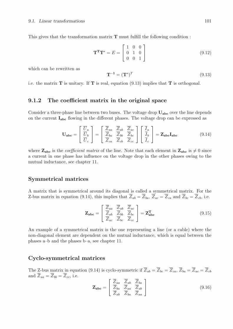
9.1. Linear transformations 101
This gives that the transformation matrix T must fulfill the following condition :
TTT∗ = E =
1 0 00 1 00 0 1
(9.12)
which can be rewritten as
T−1 = (T∗)T (9.13)
i.e. the matrix T is unitary. If T is real, equation (9.13) implies that T is orthogonal.
9.1.2 The coefficient matrix in the original space
Consider a three-phase line between two buses. The voltage drop Uabc over the line dependson the current Iabc flowing in the different phases. The voltage drop can be expressed as
Uabc =
Ua
U b
U c
=
Zaa Zab Zac
Zba Zbb Zbc
Zca Zcb Zcc
Ia
Ib
Ic
= ZabcIabc (9.14)
where Zabc is the coefficient matrix of the line. Note that each element in Zabc is 6= 0 sincea current in one phase has influence on the voltage drop in the other phases owing to themutual inductance, see chapter 11.
Symmetrical matrices
A matrix that is symmetrical around its diagonal is called a symmetrical matrix. For theZ-bus matrix in equation (9.14), this implies that Zab = Zba, Zac = Zca and Zbc = Zcb, i.e.
Zabc =
Zaa Zab Zac
Zab Zbb Zbc
Zac Zbc Zcc
= ZT
abc (9.15)
An example of a symmetrical matrix is the one representing a line (or a cable) where thenon-diagonal element are dependent on the mutual inductance, which is equal between thephases a–b and the phases b–a, see chapter 11.
Cyclo-symmetrical matrices
The Z-bus matrix in equation (9.14) is cyclo-symmetric if Zab = Zbc = Zca, Zba = Zac = Zcb
and Zaa = Zbb = Zcc, i.e.
Zabc =
Zaa Zab Zba
Zba Zaa Zab
Zab Zba Zaa
(9.16)
102 9. Analysis of three-phase systems using linear transformations
All normal three-phase systems are cyclo-symmetrical, i.e. if ia, ib, ic are permuted to ib,ic, ia, the voltages ua, ub, uc will also be permuted to ub, uc, ua. This implies that ordinaryoverhead lines, cables, transformers and electrical machines can be represented by cyclo-symmetrical matrices.
9.1.3 The coefficient matrix in the image space
If both sides of equation (9.14) are multiplied with the matrix T−1, the following is obtained
UABC = T−1Uabc = T−1ZabcIabc = (T−1ZabcT)IABC = ZABCIABC (9.17)
whereZABC = T−1ZabcT (9.18)
ZABC is the image space mapping of the coefficient matrix Zabc. This gives that if UABC
represents the image space voltages, and IABC represents the image space currents thenZABC will represent the impedances in the image space.
One motive of introducing a linear transformation may be to obtain a diagonal coefficientmatrix in the image space, i.e.
ZABC =
ZAA 0 00 ZBB 00 0 ZCC
(9.19)
By having a diagonal coefficient matrix, equation (9.17) can be rewritten as
UA = ZAAIA
UB = ZBBIB (9.20)
UC = ZCCIC
i.e. the matrix equation (9.17) having mutual couplings between the phases is replaced bythree un-coupled equations. If ZABC is diagonal as in equation (9.19), both sides in equation(9.18) can be multiplied with T and rewritten as
TZABC =
t1 t2 t3
ZAA 0 00 ZBB 00 0 ZCC
=
ZAAt1 ZBBt2 ZCCt3
=
= ZabcT = Zabc
t1 t2 t3
(9.21)
where t1, t2, t3 are columns of T. equation (9.21) can be rewritten as
Zabct1 − ZAAt1 = 0
Zabct2 − ZBBt2 = 0 (9.22)
Zabct3 − ZCCt3 = 0

9.2. Examples of linear transformations that are used in analysis of three-phase systems103
i.e. ZAA, ZBB and ZCC are the eigenvalues of matrix Zabc and the vectors t1, t2 and t3are the corresponding eigenvectors. A transformation that maps the matrix Z to a diagonalform should have a transformation matrix T having columns that are the eigenvectors of thematrix Z. Note that eigenvectors can be scaled arbitrarily.
9.2 Examples of linear transformations that are used
in analysis of three-phase systems
In the following, four commonly used linear transformations will briefly be introduced. Ingeneral, transformations can be presented in a little bit different ways in different text books.It is therefore of importance to understand the definitions used by the author.
9.2.1 Symmetrical components
In the analysis of un-symmetrical conditions in a power system, symmetrical componentsare commonly used. This complex, linear transformation use the fact that all components(lines, machines, etc.) in normal systems are cyclo-symmetrical, i.e. their impedances canbe modeled by equation (9.16). The power invariant transformation matrix and its inversefor the symmetrical components are
TS =1√3
1 1 11 α2 α1 α α2
T−1
S =1√3
1 1 11 α α2
1 α2 α
(9.23)
where α = ej120 . As given by the definition T−1S = (T∗
S)T which correspond to the as-sumption of power invarians according to equation (9.13). By using this transformation,cyclo-symmetrical matrices are transformed into a diagonal form as given in equation (9.19),i.e. the column of matrix TS consist of the eigenvectors to a cyclo-symmetrical matrix. Thiswill simplify the system analysis as indicated in equation (9.20). By using the given phasevoltage Ua, U b and U c, the power invariant symmetrical components can be calculated as
Us =
U0
U1
U2
= T−1
S Uabc =1√3
1 1 11 α α2
1 α2 α
Ua
U b
U c
(9.24)
The three components U0, U1 and U2 are called zero-sequence, positive-sequence and negative-sequence, respectively. A cyclo-symmetrical impedance matrix according to equation (9.16)can be diagonalized by using symmetrical components according to equation (9.18) as
ZS = T−1S
Zaa Zab Zba
Zba Zaa Zab
Zab Zba Zaa
TS =
Z0 0 00 Z1 00 0 Z2
(9.25)

104 9. Analysis of three-phase systems using linear transformations
where
Z0 = Zaa + Zab + Zba = zero-sequence impedance
Z1 = Zaa + α2Zab + αZba = positive-sequence impedance (9.26)
Z2 = Zaa + αZab + α2Zba = negative-sequence impedance
The three impedances Z0, Z1 and Z2 are the eigenvalues of the cyclo-symmetrical impedancematrix. For an impedance matrix that is both cyclo-symmetric and symmetric, i.e. Zba =Zab, the result after a diagonalization will be that
Z0 = Zaa + 2Zab
Z1 = Zaa − Zab (9.27)
Z2 = Zaa − Zab
Transformers, overhead lines, cables and symmetrical loads (not electrical machines) can nor-mally be represented by impedance matrices that are both symmetrical and cyclo-symmetrical,i.e. all diagonal elements are equal and all non-diagonal elements are equal. This gives thatthe positive-sequence impedance and the negative-sequence impedance are equal.
In order to make the positive-sequence phase voltage equal to the phase voltage, a referenceinvariant form of transformation for the symmetrical components is normally used. Thereference invariant transformation matrix and its inverse are
TS′ =
1 1 11 α2 α1 α α2
=
√3 ·TS T−1
S′ =1
3
1 1 11 α α2
1 α2 α
=
1√3·T−1
S (9.28)
The reference invariant transformation is not power invariant since T−1S′ = 1
3(T∗
S′)T . The
name reference invariant means that in symmetrical conditions U1 = Ua. Note that trans-formations of coefficient matrices, according to equation (9.18), are not influenced whetherthe power invariant or the reference invariant matrix is used since
ZABC(eff − inv) = T−1S ZabcTS =
(1√3T−1
S
)Zabc
(√3TS
)=
= T−1S′ ZabcTS′ = ZABC(ref − inv) (9.29)
A third variation of the transformation matrix for the symmetrical components arise whenthe ordering of the sequences is changed. If the positive-sequence is given first and thezero-sequence last, the columns of the T-matrix and the rows in the T−1 are permuted,respectively. This results in the following reference invariant transformations matrices :
TS′′ =
1 1 1α2 α 1α α2 1
T−1
S′′ =1
3
1 α α2
1 α2 α1 1 1
(9.30)
This form of the transformation matrices will be used in chapter 10 where symmetricalcomponents are discussed in more detail. The only thing that happens with the coefficientmatrix in the image space is that the diagonal elements change places.
As described above, a number of different variations of the symmetrical components canbe used, all having the same fundamental purpose, to diagonalize the cyclo-symmetricalimpedance matrices.
9.2. Examples of linear transformations that are used in analysis of three-phase systems105
9.2.2 Clarke’s components
Clarke’s components, also called α−β-components or orthogonal components, divides thosephase-quantities not having any zero-sequence into two orthogonal components. The wordzero-sequence means the same as when discussing symmetrical components, the sum of thephase components. Components not having any zero-sequence are those where the sum ofall phase components are = 0. The power invariant (T−1 = (T∗)T , see equation (9.13))transformation matrix and its inverse for the Clarke’s components are
TC =
√2
3
1√2
1 01√2−1
2
√3
21√2−1
2−√
32
T−1
C =
√2
3
1√2
1√2
1√2
1 −12
−12
0√
32
−√
32
(9.31)
Clarke’s components are a real orthogonal transformation that is mainly used in transfor-mations of time quantities, e.g.
i0(t)iα(t)iβ(t)
= i0αβ(t) = T−1
C iabc(t) =
√2
3
1√2
1√2
1√2
1 −12
−12
0√
32
−√
32
ia(t)ib(t)ic(t)
(9.32)
where i0(t) is the zero-sequence component, iα(t) is the α-component and iβ is the β-component for Clarke’s transformation of the phase currents ia(t), ib(t) and ic(t). The reasonwhy the transformation is orthogonal is given by column two and three of TC (correspondsto the α- and β-components) since the columns are orthogonal.
For a symmetrical three-phase current given by equation (3.13)
ia(t) = IM cos(ωt− φ)
ib(t) = IM cos(ωt− 120 − φ) (9.33)
ic(t) = IM cos(ωt + 120 − φ)
the Clarke’s components are given by equation (9.32)
i0(t) =1√3
(ia(t) + ib(t) + ic(t)) = 0
iα(t) =
√2
3
(ia(t)− 1
2ib(t)− 1
2ic(t)
)=
√3
2IM cos(ωt− φ) (9.34)
iβ(t) =
√2
3
(√3
2ib(t)−
√3
2ic(t)
)=
√3
2IM cos(ωt− φ− 90)
As given above, conditions not having any zero-sequence can be fully represented by Clarke’sα- and β-components. Conditions not having any zero-sequence are quite common anddepends, among other things, on the type of transformer connection used.
Matrices that are both symmetrical and cyclo-symmetrical can be diagonalized by using
106 9. Analysis of three-phase systems using linear transformations
Clarke’s transform as
ZC = T−1C
Zaa Zab Zab
Zab Zaa Zab
Zab Zab Zaa
TC =
=
Zaa + 2Zab 0 00 Zaa − Zab 00 0 Zaa − Zab
(9.35)
For this type of matrices, the diagonalizing using Clarke’s components gives exactly the sameanswer as a diagonalizing using symmetrical components, see equations (9.25) and (9.27).
This gives that the matrix representation of transformers, overhead lines, cables and sym-metrical loads (not electrical machines) can be diagonalized. The advantage of using Clarke’scomponents is that the transformation is real which gives that the mapping of real instan-taneous value mappings also are real. The disadvantage is that electrical machines cannotbe represented by three independent variables by using Clarke’s components.
Clarke’s components are used in order to simplify the analysis of e.g. multi-phase shortcircuits, transient system behavior, converter operation, etc.
9.2.3 Park’s transformation
Park’s transformation (also called dq-transformation or Blondell’s transformation) is a lineartransformation between the three physical phases and three new components. This trans-formation is often used when analyzing synchronous machines.
In Figure 9.1, a simplified description of the internal conditions of a synchronous machinehaving salient poles, is given. Two orthogonal axis are defined. One is directed along themagnetic flux induced in the rotor. The second axis is orthogonal to the first axis. Thefirst axis is called the direct-axis (d-axis) and the second axis is called the quadrature-axis(q-axis). Note that this system of coordinates follows the rotation of the rotor. The machinegiven in Figure 9.1 is a two-pole machine, but Park’s transformation can be used for machineshaving an arbitrary number of poles.
As indicated above, Park’s transformation is time independent since the displacement be-tween the dq-axes and the abc-axes is changed when the rotor revolves. The Park’s trans-formation includes not only the d- and q-components, but also the zero-sequence in orderto achieve a complete representation. The connection between phase currents ia, ib, and icand the dq0-components is given by the notation given in Figure 9.1
i0 =1√3
(ia + ib + ic)
id =
√2
3(ia cos θ + ib cos (θ − 120) + ic cos (θ + 120)) (9.36)
iq =
√2
3(−ia sin θ − ib sin (θ − 120)− ic sin (θ + 120))

9.2. Examples of linear transformations that are used in analysis of three-phase systems107
Direction ofrotation
n′
ia
fasa
sc
sb
iQ
θ
q-axis
a-axis
d-axis
b-axis
c-axis
iQ
iD
iD
iF
iF
ib
fb n′
n′fc
ic
ω
d
d-axel
q-axel
q Q
F
D
Figure 9.1. Definitions of quantities in Park’s transformation
This equation can be written on matrix form as
i0dq =
i0idiq
=
√2
3
1√2
1√2
1√2
cos θ cos (θ − 120) cos (θ + 120)− sin θ − sin (θ − 120) − sin (θ + 120)
iaibic
= T−1
P iabc
(9.37)The matrix TP and matrix T−1
P can be transposed as
TP = (T−1P )−1 =
√2
3
1√2
cos θ − sin θ1√2
cos (θ − 120) − sin (θ − 120)1√2
cos (θ + 120) − sin (θ + 120)
= (T−1
P )T (9.38)
The transformation is hence power invariant according to equation (9.13). Park’s transfor-mation is real and usable when transforming time quantities. Note that the Park’s trans-formation is linear but the transformation matrix is time dependent. At constant frequencyθ = ωt + θ0.
The Park’s transformation is a frequency transformed version of Clarke’s transformation.When θ = 0 (Park’s transformation), the transformation matrices are identical, i.e. TC =TP(θ = 0).
9.2.4 Phasor components
Phasor components are mainly used at instantaneous value analysis when a single machineor when several machines are connected together. The power invariant (T−1 = (T∗)T , see
108 9. Analysis of three-phase systems using linear transformations
equation (9.13)) transformation matrix and its inverse for these components are
TR =1√3
1 ejθ e−jθ
1 α2ejθ αe−jθ
1 αejθ α2e−jθ
(9.39)
T−1R =
1√3
1 1 1e−jθ αe−jθ α2e−jθ
ejθ α2ejθ αejθ
where α = ej120 . The phasor components of the three-phase currents ia(t), ib(t) and ic(t)can be obtained as
i0(t)is(t)iz(t)
= i0sz(t) = T−1
R iabc(t) =1√3
1 1 1e−jθ αe−jθ α2e−jθ
ejθ α2ejθ αejθ
ia(t)ib(t)ic(t)
(9.40)
where i0(t) is the zero-sequence component and is(t) is called the field vector current, thecomplex phasor of the current. The current is(t) is complex since the transformation matrixis complex. By assuming that ia(t), ib(t) and ic(t) are real, the expression for iz(t) can bewritten as
iz(t) =1√3ejθ
(ia(t) + α2ib(t) + αic(t)
)= (9.41)
=
[1√3e−jθ
(ia(t) + αib(t) + α2ic(t)
)]∗= i
∗s(t)
i.e. iz(t) is known if the field vector is(t) is known. Under conditions of no zero-sequencecomponents, the field vector is fully describing an arbitrary real three-phase quantity.
For a symmetrical three-phase current as given in equation (9.33), the phasor componentscan be obtained according to equation (9.40)
i0(t) =1√3
(ia(t) + ib(t) + ic(t)) = 0
is(t) =e−jθ
√3
(ia(t) + αib(t) + α2ic(t)
)=
√3
2IMej(ωt−φ−θ) (9.42)
iz(t) =ejθ
√3
(ia(t) + α2ib(t) + αic(t)
)=
√3
2IMe−j(ωt−φ−θ) = i
∗s(t)
Finally, for θ = ωt the following is obtained
i0(t) = 0
is(t) =
√3
2IMe−jφ (9.43)
iz(t) =
√3
2IMejφ = i
∗s(t)
i.e. the field vector current is(t) has a constant magnitude, independent of time.

9.2. Examples of linear transformations that are used in analysis of three-phase systems109
By assuming real phase currents having no zero-sequence, they can be calculated by usingthe field vector current as
ia(t)ib(t)ic(t)
= TRi0sz(t) =
1√3
1 ejθ e−jθ
1 α2ejθ αe−jθ
1 αejθ α2e−jθ
0is(t)
i∗s(t)
= (9.44)
=1√3
[ejθis(t)
]+
[ejθis(t)
]∗[α2ejθis(t)
]+
[α2ejθis(t)
]∗[αejθis(t)
]+
[α2ejθis(t)
]∗
=
2√3
Re[ejθis(t)
]Re
[α2ejθis(t)
]Re
[αejθis(t)
]
Phasor components are a frequency transformed form of the symmetrical components. Forθ = 0 (phasor components), the transformation matrix for the phasor components and thesymmetrical components are identical, i.e. TR(θ = 0) = TS.

110 9. Analysis of three-phase systems using linear transformations
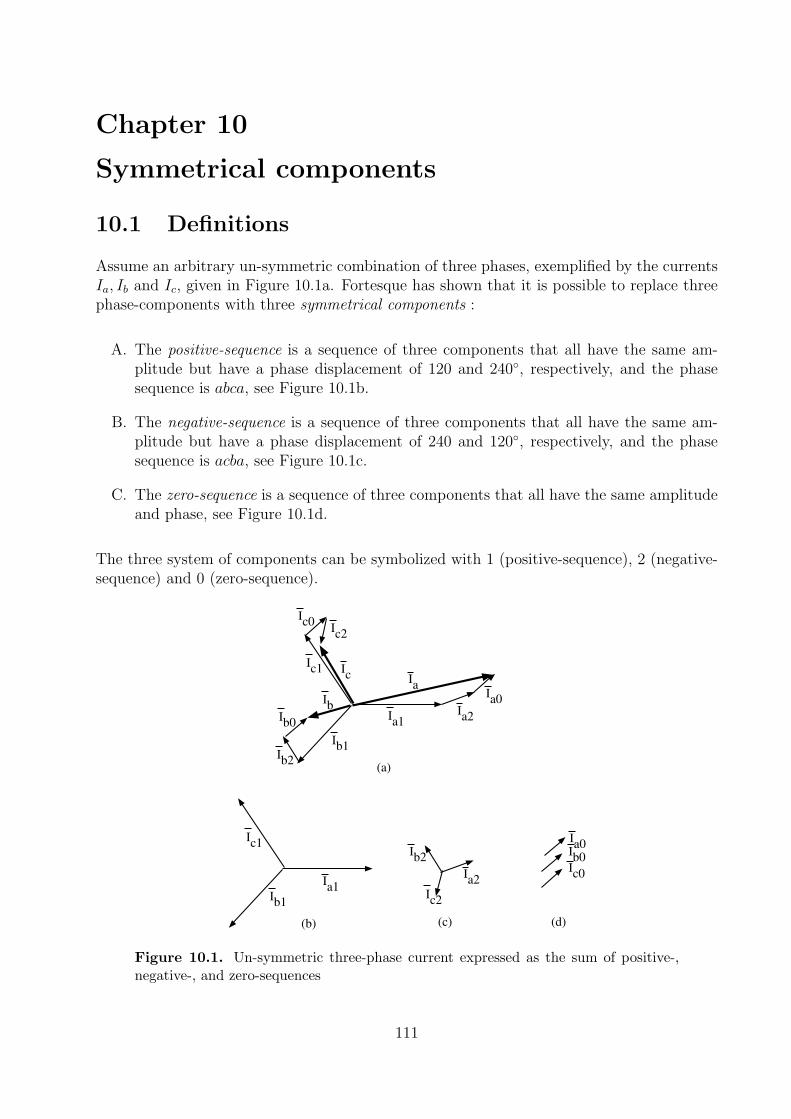
Chapter 10
Symmetrical components
10.1 Definitions
Assume an arbitrary un-symmetric combination of three phases, exemplified by the currentsIa, Ib and Ic, given in Figure 10.1a. Fortesque has shown that it is possible to replace threephase-components with three symmetrical components :
A. The positive-sequence is a sequence of three components that all have the same am-plitude but have a phase displacement of 120 and 240, respectively, and the phasesequence is abca, see Figure 10.1b.
B. The negative-sequence is a sequence of three components that all have the same am-plitude but have a phase displacement of 240 and 120, respectively, and the phasesequence is acba, see Figure 10.1c.
C. The zero-sequence is a sequence of three components that all have the same amplitudeand phase, see Figure 10.1d.
The three system of components can be symbolized with 1 (positive-sequence), 2 (negative-sequence) and 0 (zero-sequence).
Ia
Ia1
Ia1
Ia2
Ia0
Ia2
Ia0
Ib1
Ib1
Ic1
Ic1
Ic0
Ic2
Ib2
Ib2
Ib0
Ic2
Ic
Ib
Ib0
Ic0
(b) (c) (d)
(a)
Figure 10.1. Un-symmetric three-phase current expressed as the sum of positive-,negative-, and zero-sequences
111

112 10. Symmetrical components
The result shown in Figure 10.1 can mathematically be expressed as :
Ia = Ia1 + Ia2 + Ia0
Ib = Ib1 + Ib2 + Ib0 (10.1)
Ic = Ic1 + Ic2 + Ic0
The three positive-sequence components can be denoted as
Ib1 = Ia1e−j120 (10.2)
Ic1 = Ia1ej120
The corresponding expressions for the negative- and zero-sequence are as
Ib2 = Ia2ej120
Ic2 = Ia2e−j120 (10.3)
Ia0 = Ib0 = Ic0
By inserting equation (10.2) and (10.3) into equation (10.1), the following is obtained
Ia = Ia1 + Ia2 + Ia0
Ib = α2Ia1 + αIa2 + Ia0 (10.4)
Ic = αIa1 + α2Ia2 + Ia0
In order to simplify the expressions, the symbol α has been introduced
α = ej120 = cos 120 + j sin 120 = −1
2+ j
√3
2(10.5)
The following expressions of the symbol α are valid
α2 = ej240 = e−j120 = −1
2− j
√3
2α3 = 1
1 + α + α2 = 0 (10.6)
α∗ = α2
(α2)∗ = α
Equation (10.4) can, by using matrix form, be written as
If = TIs (10.7)
where the matrix
T =
1 1 1α2 α 1α α2 1
(10.8)

10.1. Definitions 113
which is called the transformation matrix for the symmetrical components. This matrix isequal to the reference invariant matrix TS′′ according to equation (9.30). The current vector
If =
Ia
Ib
Ic
(10.9)
represents the phase components of the current whereas
Is =
Ia1
Ia2
Ia0
or shorter Is =
I1
I2
I0
(10.10)
represents the symmetrical components of the current.
By using equation (10.7), the symmetrical components as a function of phase componentscan be obtained :
Is = T−1If (10.11)
where
T−1 =1
3
1 α α2
1 α2 α1 1 1
(10.12)
which is equal to T−1S′′ according to equation (9.30). Of course, the symmetrical components
can also be applied to voltages. Using the vectors
Uf =
Ua
U b
U c
and Us =
Ua1
Ua2
Ua0
or shorter Us =
U1
U2
U0
(10.13)
for representing phase-quantities and symmetrical components, respectively, the relationbetween them can be written as
Uf = TUs (10.14)
Us = T−1Uf (10.15)
Example 10.1 Calculate the symmetrical components for the following symmetrical voltages
Uf =
Ua
U b
U c
=
277 6 0
2776 − 120
2776 + 120
V (10.16)
Solution
By using equation (10.12) and (10.15), the symmetrical components of the voltage Uf can

114 10. Symmetrical components
be calculated as
U1
U2
U0
= Us = T−1Uf =
1
3
1 α α2
1 α2 α1 1 1
Ua
U b
U c
= (10.17)
=1
3
1 · 277 + 1 6 120 · 2776 − 120 + 1 6 240 · 277 6 + 120
1 · 277 + 1 6 240 · 2776 − 120 + 1 6 120 · 277 6 + 120
1 · 277 + 1 · 2776 − 120 + 1 · 277 6 + 120
=
=
2776 0
00
As given in the example, a symmetric three-phase system with a phase sequence of abc givesrise to a positive-sequence voltage only, having the same amplitude and angle as the voltagein phase a.
Example 10.2 For a Y-connected three-phase load with zero conductor, phase b is at oneoccasion disconnected. The load currents at that occasion is :
If =
Ia
Ib
Ic
=
106 0
010 6 + 120
A (10.18)
Calculate the symmetrical components of the load current as well as the current in the zeroconductor, In.
Solution
I1
I2
I0
=
1
3
1 · 10 6 0 + 1 6 120 · 0 + 1 6 240 · 106 + 120
1 · 10 6 0 + 1 6 240 · 0 + 1 6 120 · 106 + 120
1 · 10 6 0 + 1 · 0 + 1 · 106 + 120
= (10.19)
=
6.6676 0
3.3336 − 60
3.333 6 60
In = Ia + Ib + Ic = 10 6 0 + 0 + 10 6 + 120 = 10 6 60 = 3I0 (10.20)
As given in the example, the current in the zero conductor is three times as large as thezero-sequence current.
10.2 Power calculations in un-symmetrical conditions
The three-phase complex power of the phase-components can be calculated as
S = P + jQ = UaI∗a + U bI
∗b + U cI
∗c = UT
f I∗f (10.21)

10.2. Power calculations in un-symmetrical conditions 115
By introducing symmetrical components, the expression above can be converted to
S = UTf I∗f = (TUs)
T(TIs)∗ = UT
s TTT∗I∗s (10.22)
The expression TTT∗ can be written as
TTT∗ =
1 α2 α1 α α2
1 1 1
1 1 1α α2 1α2 α 1
= 3
1 0 00 1 00 0 1
(10.23)
i.e. the transformation is not power invariant, see subsection 9.1.1, equation (9.12). Equation(10.22) can be rewritten as
S = 3UTs I∗s = 3U s1I
∗s1 + 3U s2I
∗s2 + 3U s0I
∗s0 (10.24)
Since the magnitude of the phase-to-phase voltages are√
3 times larger than the phase-to-ground voltages and Sb =
√3 · Ub · Ib, the introduction of the per-unit system gives that
equation (10.24) can be rewritten as
Spu =
√3(√
3Us)T · I∗s√
3 · Ub · Ib
= U s1−puI∗s1−pu + U s2−puI
∗s2−pu + U s0−puI
∗s0−pu (10.25)
This implies that the total power in an un-symmetric system can be calculated as the sumof the powers in the positive-, negative-, and zero-sequences.

116 10. Symmetrical components

K Chapter 11
Line model for un-symmetric three-phaseconditions
11.1 Series impedance of single-phase overhead line
The theory of having an overhead line using the ground as a return conductor was discussedby Carson in 1923. Carson considered a single conductor a of unity length (e.g. one meter)running in parallel with the ground, see Figure 11.1.
a
+
−aU
+
−
Local earthRef. Surface ofremote earth0dU =
d d ′Fictitious groundreturn conductora′aaZ
ddZ
aI
d aI I= −
adD adZ1 Unit
Figure 11.1. Carson’s single-phase overhead line using the ground as return path
The current Ia flows in the conductor using the ground between d− d′ as return path. Theground is assumed to have an uniform resistance and an infinite extension. The current Id
(=−Ia) is distributed over a large area, flowing along the ways of least resistance. Kirchhoff’slaw about the same voltage drop along each path is fulfilled. It has been shown that thesedistributed return paths may, in the analysis, be replaced by a single return conductor havinga radius = rd located at a distance Dad from the overhead line according to Figure 11.1. Thedistance Dad is a function of the resistivity of the ground ρ. The distance Dad increases asthe resistivity ρ increases.
The inductance of this circuit can be calculated as
La =µ
2πln
1
Da︸ ︷︷ ︸Laa
+µ
2πln
1
Dd︸ ︷︷ ︸Ldd
−2µ
2πln
1
Dad︸ ︷︷ ︸Lad
=µ
2π
(ln
Dad
Da
+ lnDad
Dd
)(11.1)
where
µ = the permeability of the conductor
Da = e−1/4ra for a single conductor with radius ra
Dd = e−1/4rd for a return conductor in ground with radius rd
The inductance can according to equation (11.1) be divided into three parts, two apparent selfinductances (Laa, Ldd) and one apparent mutual inductance (Lad). Note that these quantities
117

118 11. Line model for un-symmetric three-phase conditions
are only mathematical quantities without any physical meaning. For instance, they havewrong dimension inside the ln-sign. It is only after the summation they achieve a physicalmeaning. Hopefully, the different part expressions will simplify the understanding of thebehavior of a three-phase line. The total series reactance of this single-phase conductor is
Xa = ωLa = ω(Laa + Ldd − 2Lad) (11.2)
By using this line model, having apparent inductances, the voltage drop for a single-phaseline can be calculated as
[Uaa′
Udd′
]=
[Ua − Ua′
Ud − Ud′
]=
[zaa zad
zad zdd
] [Ia
−Ia
]volt/length unit (11.3)
where Ua, Ua′ , Ud and Ud′ are given in proportion to the same reference. Since Ud = 0 andUa′ − Ud′ = 0, Ua can be obtained by subtracting the two equations from each other :
Ua = (zaa + zdd − 2zad)Ia = ZaIa (11.4)
By definitionZa ≡ zaa + zdd − 2zad Ω/length unit (11.5)
The impedances in this equation can be calculated as
zaa = ra + jxaa = ra + jωLaa Ω/length unit
zdd = rd + jxdd = rd + jωLdd Ω/length unit (11.6)
zad = jxad = jωLad Ω/length unit
Za = ra + rd + jXa Ω/length unit
where
ra = conductor resistance per length unit
rd = ground resistance per length unit
11.2 Series impedance of a three-phase overhead line
In order to obtain the series impedance of a three-phase line, the calculations are performedin the same way as for the single-phase line. In Figure 11.2, the impedances, voltages andcurrents of the line are given.
Since all conductors are grounded at a′, b′, c′, the following are valid
Id = −(Ia + Ib + Ic) (11.7)
Ua′ − Ud′ = 0 U b′ − Ud′ = 0 U c′ − Ud′ = 0
The voltage drop over the conductors can be calculated as
Uaa′
U bb′
U cc′
Udd′
=
Ua − Ua′
U b − U b′
U c − U c′
Ud − Ud′
=
zaa zab zac zad
zab zbb zbc zbd
zac zbc zcc zcd
zad zbd zcd zdd
Ia
Ib
Ic
Id
volt/length unit (11.8)
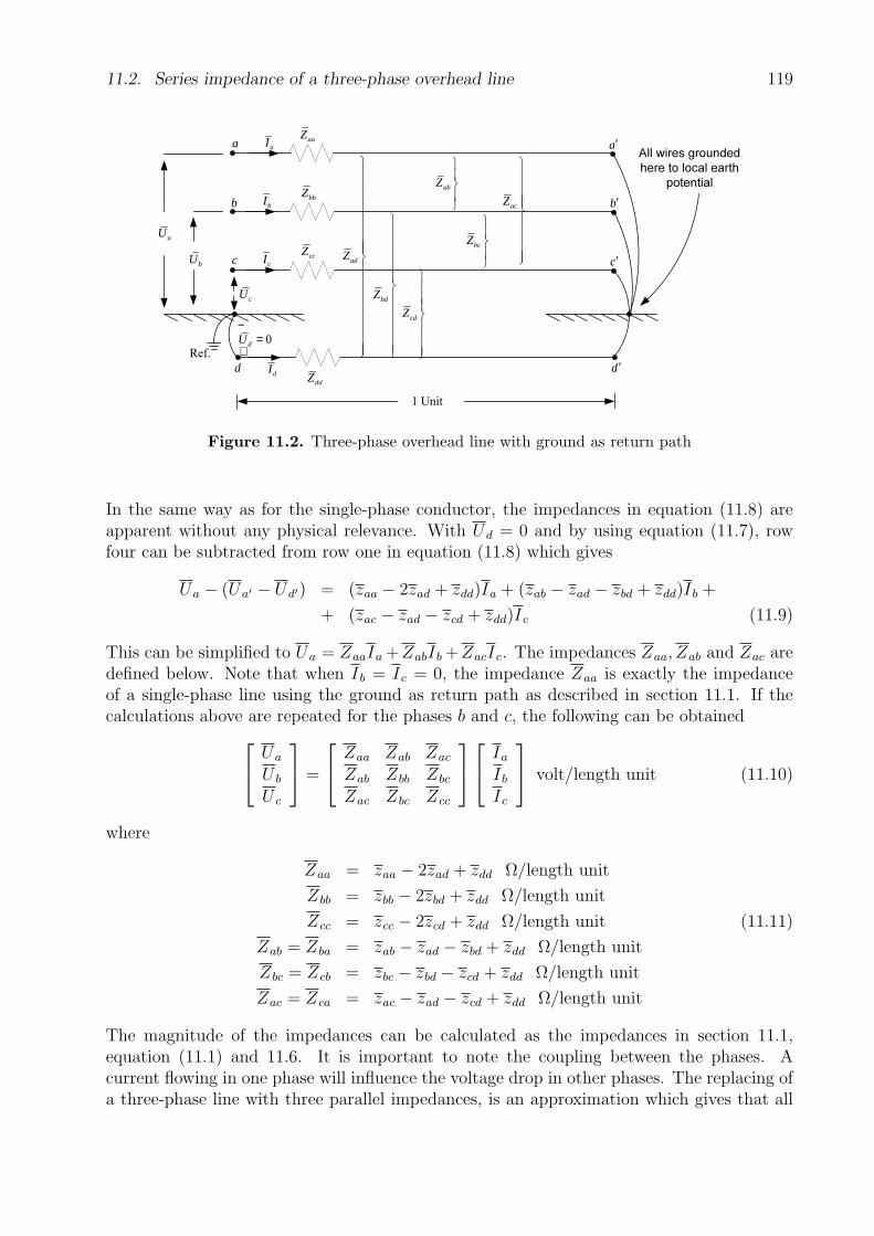
11.2. Series impedance of a three-phase overhead line 119
All wires groundedhere to local earth
potential
adZ
ddZdI
a aI
d+
−
Ref.0dU =
ccZc cI
aaZ
bbZb bI
d ′
c′
a′
b′
1 Unit
cU
aU
bU
bdZ
cdZ
abZ
bcZ
acZ
Figure 11.2. Three-phase overhead line with ground as return path
In the same way as for the single-phase conductor, the impedances in equation (11.8) areapparent without any physical relevance. With Ud = 0 and by using equation (11.7), rowfour can be subtracted from row one in equation (11.8) which gives
Ua − (Ua′ − Ud′) = (zaa − 2zad + zdd)Ia + (zab − zad − zbd + zdd)Ib +
+ (zac − zad − zcd + zdd)Ic (11.9)
This can be simplified to Ua = ZaaIa +ZabIb +ZacIc. The impedances Zaa, Zab and Zac aredefined below. Note that when Ib = Ic = 0, the impedance Zaa is exactly the impedanceof a single-phase line using the ground as return path as described in section 11.1. If thecalculations above are repeated for the phases b and c, the following can be obtained
Ua
U b
U c
=
Zaa Zab Zac
Zab Zbb Zbc
Zac Zbc Zcc
Ia
Ib
Ic
volt/length unit (11.10)
where
Zaa = zaa − 2zad + zdd Ω/length unit
Zbb = zbb − 2zbd + zdd Ω/length unit
Zcc = zcc − 2zcd + zdd Ω/length unit (11.11)
Zab = Zba = zab − zad − zbd + zdd Ω/length unit
Zbc = Zcb = zbc − zbd − zcd + zdd Ω/length unit
Zac = Zca = zac − zad − zcd + zdd Ω/length unit
The magnitude of the impedances can be calculated as the impedances in section 11.1,equation (11.1) and 11.6. It is important to note the coupling between the phases. Acurrent flowing in one phase will influence the voltage drop in other phases. The replacing ofa three-phase line with three parallel impedances, is an approximation which gives that all

120 11. Line model for un-symmetric three-phase conditions
non-diagonal element of the Z-bus matrix in equation (11.10) are neglected. In other words,the mutual inductance between the conductors are neglected. The error this simplificationgives is dependent on several things, e.g. the distance between the conductors, the length ofthe conductors and the magnitude of the currents in the conductors.
11.2.1 Symmetrical components of the series impedance of a three-phase line
Symmetrical components are often used in the analysis of power systems having three-phaselines, in order to simplify the complicated cross-couplings that exist between the phases.The quantities in equation (11.10) can be defined as :
Ua
U b
U c
= Uf = ZfIf =
Zaa Zab Zac
Zab Zbb Zbc
Zac Zbc Zcc
Ia
Ib
Ic
(11.12)
The voltage phase vectors (Uf ) and current vectors (If ) can be replaced by the correspondingsymmetrical component multiplied with matrix T according to the section on symmetricalcomponents :
Uf = TUs = ZfTIs = ZfIf (11.13)
This equation can be rewritten as
Us = T−1ZfTIs = ZsIs (11.14)
If a symmetrical overhead line (or cable) is assumed, i.e. Zaa = Zbb = Zcc and Zab = Zbc =Zac, the following is obtained
Zs = T−1ZfT =1
3
1 α α2
1 α2 α1 1 1
Zaa Zab Zac
Zab Zbb Zbc
Zac Zbc Zcc
1 1 1α2 α 1α α2 1
=
=
Zaa − Zab 0 00 Zaa − Zab 00 0 Zaa + 2Zab
(11.15)
Equation (11.14) can be rewritten as
U1
U2
U0
= Us = ZsIs = (11.16)
=
Zaa − Zab 0 00 Zaa − Zab 00 0 Zaa + 2Zab
I1
I2
I0
=
Z1I1
Z2I2
Z0I0
where
Z1 = Zaa − Zab = positive-sequence impedance
Z2 = Zaa − Zab = negative-sequence impedance (11.17)
Z0 = Zaa + 2Zab = zero-sequence impedance

11.2. Series impedance of a three-phase overhead line 121
By inserting the expressions used in equation (11.11) into equation (11.17), the followingcan be obtained
Z1 = Z2 = zaa − zab (11.18)
Z0 = zaa + 2zab − 6zad + 3zdd
Note that the coupling to ground are not present in the expressions for the positive- andnegative-sequence impedances, i.e. the elements having index d in the Z-bus matrix inequation (11.8) are not included. This means that the zero-sequence current is zero in thepositive- and negative-sequence reference frame, which is quite logical. All couplings toground are represented in the zero-sequence impedance. As indicated above, a line by usingthis model, can be represented as three non-coupled components : positive-, negative-, andzero-sequence components. It should be pointed out that some loss of information will occurwhen using this model. For example, if only positive-, negative-, and zero-sequence data aregiven, the potential of the ground, Ud′ in Figure 11.2, cannot be calculated. To calculatethat potential, more detailed data are needed. The line model introduced in section 7.2, isbased on positive-sequence data only, since symmetrical conditions are assumed.
11.2.2 Equivalent diagram of the series impedance of a line
As given above, for a symmetrical line Z1 = Z2. Assume that this line can be replaced by anequivalent circuit according to Figure 11.3, i.e. three phase impedances Zα and one return
Zβ
Zα
Zα
Zα
aI
bI
cI
oI
aU
cU
bU
oU
aU ′
bU ′
oU ′
cU ′
Figure 11.3. Equivalent diagram of the series impedance of a line
impedance Zβ where the mutual inductance between the phases = 0. With three phases andone return path, as given by the equivalent in Figure 11.3, the following is valid
I0 = Ia + Ib + Ic (11.19)
By using equation (11.19), the voltage drop between the phases and the return conductorcan be calculated as
U′a − U
′0 = Ua − U0 − Ia · Zα − (Ia + Ib + Ic)Zβ
U′b − U
′0 = U b − U0 − Ib · Zα − (Ia + Ib + Ic)Zβ (11.20)
U′c − U
′0 = U c − U0 − Ic · Zα − (Ia + Ib + Ic)Zβ
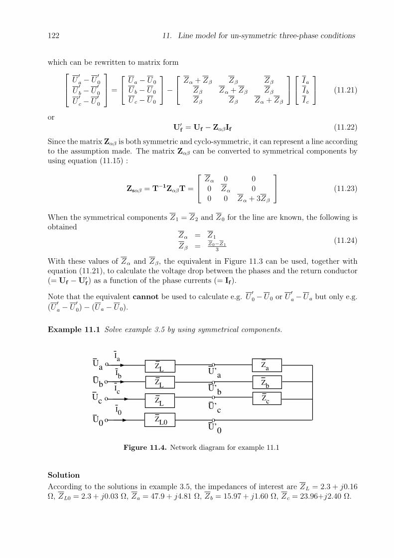
122 11. Line model for un-symmetric three-phase conditions
which can be rewritten to matrix form
U′a − U
′0
U′b − U
′0
U′c − U
′0
=
Ua − U0
U b − U0
U c − U0
−
Zα + Zβ Zβ Zβ
Zβ Zα + Zβ Zβ
Zβ Zβ Zα + Zβ
Ia
Ib
Ic
(11.21)
or
U′f = Uf − ZαβIf (11.22)
Since the matrix Zαβ is both symmetric and cyclo-symmetric, it can represent a line accordingto the assumption made. The matrix Zαβ can be converted to symmetrical components byusing equation (11.15) :
Zsαβ = T−1ZαβT =
Zα 0 00 Zα 00 0 Zα + 3Zβ
(11.23)
When the symmetrical components Z1 = Z2 and Z0 for the line are known, the following isobtained
Zα = Z1
Zβ = Z0−Z1
3
(11.24)
With these values of Zα and Zβ, the equivalent in Figure 11.3 can be used, together withequation (11.21), to calculate the voltage drop between the phases and the return conductor(= Uf −U′
f ) as a function of the phase currents (= If ).
Note that the equivalent cannot be used to calculate e.g. U′0−U0 or U
′a−Ua but only e.g.
(U′a − U
′0)− (Ua − U0).
Example 11.1 Solve example 3.5 by using symmetrical components.
o
o
o
o
o
o
o
o
ZL
ZL
ZL
ZL0
Za
Zb
Zc
Ib
Ic
I0
Ia
Ua
Ub
Uc
U0
U’0
U’c
U’b
U’a
Figure 11.4. Network diagram for example 11.1
Solution
According to the solutions in example 3.5, the impedances of interest are ZL = 2.3 + j0.16Ω, ZL0 = 2.3 + j0.03 Ω, Za = 47.9 + j4.81 Ω, Zb = 15.97 + j1.60 Ω, Zc = 23.96+j2.40 Ω.

11.2. Series impedance of a three-phase overhead line 123
The symmetrical components of the line will first be calculated. Note that the line in theexample is given in the same way as the equivalent. The symmetrical components can becalculated by using equation (11.23) :
Z1 = Z2 = ZL = 2.3 + j0.16 ΩZ0 = ZL + 3ZL0 = 9.2 + j0.25 Ω
(11.25)
which gives that
Zs =
Z1 0 00 Z2 00 0 Z0
=
2.3 + j0.16 0 00 2.3 + j0.16 00 0 9.2 + j0.25
(11.26)
The symmetrical components for the load can be calculated by using equation (11.15)
ZLDS =1
3
1 α α2
1 α2 α1 1 1
Za 0 00 Zb 00 0 Zc
1 1 1α2 α 1α α2 1
=
=
29.28 + j2.94 9.09 + j3.24 9.55− j1.379.55− j1.37 29.28 + j2.94 9.09 + j3.249.09 + j3.24 9.55− j1.37 29.28 + j2.94
Ω (11.27)
The applied voltage is symmetric, i.e. it has only one sequence, the positive one :
US = T−1Uf =
220 6 0
00
V (11.28)
The equation for this un-symmetric three-phase network can be described as
US = (Zs + ZLDS)IS (11.29)
which can be rewritten as
IS = (Zs + ZLDS)−1US =
8.116 − 5.51
2.226 149.09
1.756 − 155.89
A (11.30)
The symmetrical components for the voltage at the load can be calculated as
ULDs = ZLDSIS =
201.326 − 0.14
5.136 − 26.93
16.106 25.67
V (11.31)
The power obtained in the radiators can be calculated by using equation (10.24)
S = 3UTLDsI
∗s = 4754 + j477 VA (11.32)
i.e. the thermal power is 4754 W.

124 11. Line model for un-symmetric three-phase conditions
As given above, only the voltage drop at the load and the load currents can be calculated byusing the symmetrical components. The ground potential at the load cannot be calculated,but that is usually of no interest.
Previously, in example 3.5, 5.1 and 5.2, the ground potential at the load has been calculatedby using other types of circuit analyses. It should be pointed out that the value of the groundpotential has no physical interpretation if the value of ZL and ZL0 has been obtained byusing the symmetrical components of the line according to equation (11.24). As given bythe solutions, the load demand, phase voltages at the load and the currents at the load arephysically correct by using either one of the four methods of solution.
11.3 Shunt capacitance of a three-phase line
The line resistance and inductance are components that together form the series impedanceof the line. The capacitance that is of interest in this section, forms the shunt component.
The series component, usually the inductance, gives a limit on the maximum amount of thecurrent that can be transmitted over the line, and by that also the maximum power limit.The capacitive shunt component behaves as a reactive power source. The reactive powergenerated, is proportional to the voltage squared, which implies that the importance of theshunt capacitance increases with the voltage level. For lines having a nominal voltage of300–500 kV and a length of more than 200 km, these capacitances are of great importance.In high voltage cables where the conductors are more close to one another, the capacitanceis up to 20–40 times larger than for overhead lines. The reactive power generation can be aproblem in cables having a length of only 10 km.
There is a fundamental law about electric fields saying that the electric potential v at acertain point on the distance r from a point charge q, can be calculated as :
v =q
4πε0rV (11.33)
where ε0 = 8.854× 10⁻¹² F/m, permittivity of vacuum. This law gives that there is a directrelationship between the difference in potential and accumulation of charges. If two long,parallel conductors are of interest, and if there is a voltage difference, v1 − v2, between thelines, an accumulation of charges with different sign, +Q and −Q, will take place. Themagnitude of the total charge Q depends mainly on the distance between the lines but alsoon the design of the lines. For cables, the material between the conductors will also have aninfluence on the charge accumulation. The capacitance between the two conductors is equalto the quotient between the charge Q and the difference in potential :
C ≡ Q
v1 − v2
(11.34)
For a three-phase line, the corresponding capacitance is located between all conductors.When having a difference in potential between a conductor and ground, an accumulation ofcharges will also occur in relation to the magnitude of the capacitance. In Figure 11.5, thedifferent capacitances of a three-phase overhead line are given. A line is normally constructed

11.3. Shunt capacitance of a three-phase line 125
Figure 11.5. Capacitances of a three-phase overhead line without earth wires
in a symmetrical way, i.e. the mean distance between the phases are equal. Also, themean distance between a phase and ground is the same for all phases. In Figure 11.5, thiscorresponds to the case that cab = cbc = cac and cag = cbg = ccg when the entire line is ofinterest.
In the same way as given earlier for the series impedances, the positive-, negative- andzero-sequence capacitances can be calculated. Only the results from the calculations will bepresented here.
C1 = C2 =2πε0
ln[
2HaAr
] F/m (11.35)
C0 =2πε0
ln[
2HA2
ra2
] F/m (11.36)
where, according to Figure 11.6
C1 = positive-sequence capacitance
C2 = negative-sequence capacitance
C0 = zero-sequence capacitance
H = 3√
H1H2H3
A = 3√
A1A2A3
a = 3√
a12a13a23
r = the equivalent radius of the line = e−1/4 · real radius of the line
Note that C1 is equal to C2, but C0 has a different value. When having a closer lookat the equations for C1, it can be seen that 2H/A ≈ 1 according to Figure 11.6, whichmeans that the distance to ground has a relatively small influence. If the conductors arelocated close to one another, then 2H = A. The line model described in section 7.2, usesonly the positive-sequence capacitance C1 for the line. In principle, this can be regardedas a ∆-Y-transformation of the capacitances between the phases since they are the maincontributors to the positive- and negative-sequence capacitances. The coupling to ground isof less importance. In cables, the positive- and negative-sequence capacitances are usuallyhigher owing to the short distance between the phases.
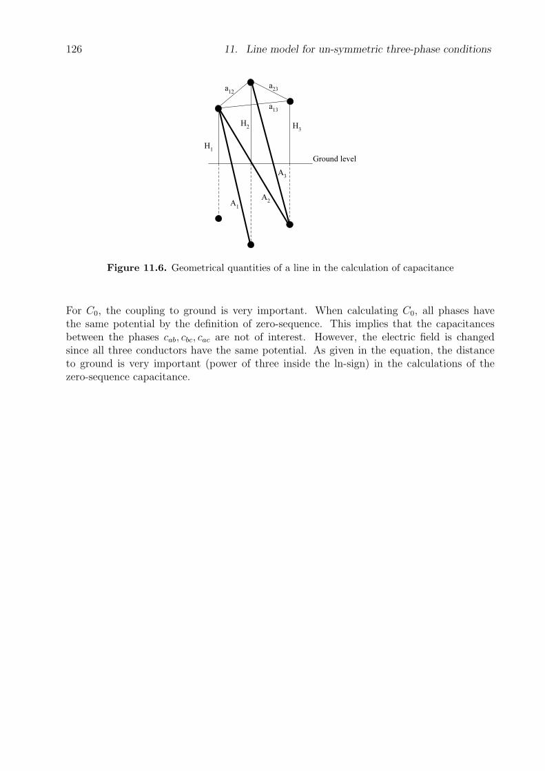
126 11. Line model for un-symmetric three-phase conditions
Ground levelH1
H2 H3
a12 a23
a13
A1A2
A3
Figure 11.6. Geometrical quantities of a line in the calculation of capacitance
For C0, the coupling to ground is very important. When calculating C0, all phases havethe same potential by the definition of zero-sequence. This implies that the capacitancesbetween the phases cab, cbc, cac are not of interest. However, the electric field is changedsince all three conductors have the same potential. As given in the equation, the distanceto ground is very important (power of three inside the ln-sign) in the calculations of thezero-sequence capacitance.

Chapter 12
Transformer model in un-symmetricthree-phase conditions
In the analysis of un-symmetric conditions in three-phase circuits, the transformer is repre-sented by its positive-, negative- and zero-sequence impedances. These can be determinedby analyzing the three-phase transformer, e.g. the Y-∆-coupling shown in Figure 12.1.Three single-phase transformers are used in this coupling and the zero connection point is
Figure 12.1. Y-∆-coupled transformer to determine the positive-, negative- and zero-sequence impedances
grounded via an impedance Zn. The impedance Ze represents the equivalent impedanceof each single-phase transformer and consists of both leakage reactance of the primary andsecondary winding as well as the resistance of the windings. The magnetizing current of thetransformer can be neglected, i.e. the magnetizing impedance is assumed to be infinitelylarge.
By using the direction of currents as given in Figure 12.1, the following expressions for thethree phases of the transformer can be held
∆Ua = IaZe + InZn
∆U b = IbZe + InZn (12.1)
∆U c = IcZe + InZn
127
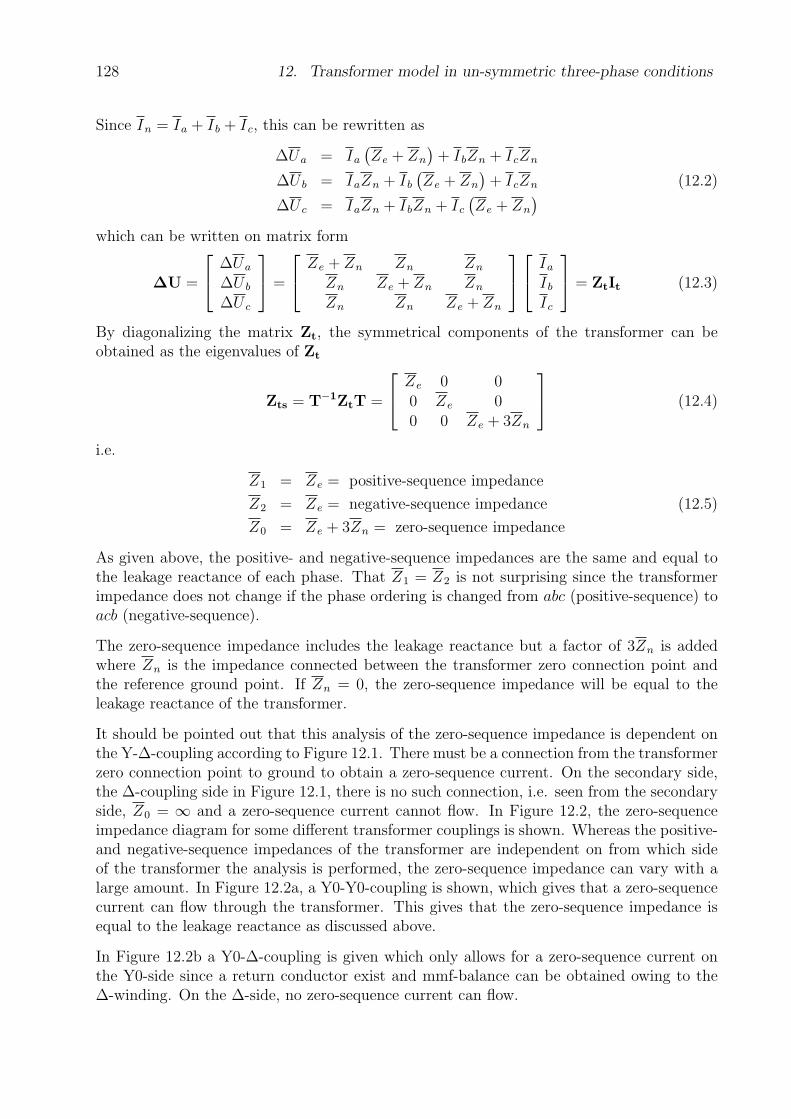
128 12. Transformer model in un-symmetric three-phase conditions
Since In = Ia + Ib + Ic, this can be rewritten as
∆Ua = Ia
(Ze + Zn
)+ IbZn + IcZn
∆U b = IaZn + Ib
(Ze + Zn
)+ IcZn (12.2)
∆U c = IaZn + IbZn + Ic
(Ze + Zn
)
which can be written on matrix form
∆U =
∆Ua
∆U b
∆U c
=
Ze + Zn Zn Zn
Zn Ze + Zn Zn
Zn Zn Ze + Zn
Ia
Ib
Ic
= ZtIt (12.3)
By diagonalizing the matrix Zt, the symmetrical components of the transformer can beobtained as the eigenvalues of Zt
Zts = T−1ZtT =
Ze 0 00 Ze 00 0 Ze + 3Zn
(12.4)
i.e.
Z1 = Ze = positive-sequence impedance
Z2 = Ze = negative-sequence impedance (12.5)
Z0 = Ze + 3Zn = zero-sequence impedance
As given above, the positive- and negative-sequence impedances are the same and equal tothe leakage reactance of each phase. That Z1 = Z2 is not surprising since the transformerimpedance does not change if the phase ordering is changed from abc (positive-sequence) toacb (negative-sequence).
The zero-sequence impedance includes the leakage reactance but a factor of 3Zn is addedwhere Zn is the impedance connected between the transformer zero connection point andthe reference ground point. If Zn = 0, the zero-sequence impedance will be equal to theleakage reactance of the transformer.
It should be pointed out that this analysis of the zero-sequence impedance is dependent onthe Y-∆-coupling according to Figure 12.1. There must be a connection from the transformerzero connection point to ground to obtain a zero-sequence current. On the secondary side,the ∆-coupling side in Figure 12.1, there is no such connection, i.e. seen from the secondaryside, Z0 = ∞ and a zero-sequence current cannot flow. In Figure 12.2, the zero-sequenceimpedance diagram for some different transformer couplings is shown. Whereas the positive-and negative-sequence impedances of the transformer are independent on from which sideof the transformer the analysis is performed, the zero-sequence impedance can vary with alarge amount. In Figure 12.2a, a Y0-Y0-coupling is shown, which gives that a zero-sequencecurrent can flow through the transformer. This gives that the zero-sequence impedance isequal to the leakage reactance as discussed above.
In Figure 12.2b a Y0-∆-coupling is given which only allows for a zero-sequence current onthe Y0-side since a return conductor exist and mmf-balance can be obtained owing to the∆-winding. On the ∆-side, no zero-sequence current can flow.

129
Coupling Equivalent zero sequencediagram
Figure 12.2. Zero-sequence diagrams for different transformer couplings
In Figure 12.2c–e, no zero-sequence current can flow on either side due to the connectiontypes.

130 12. Transformer model in un-symmetric three-phase conditions

Chapter 13
Analysis of un-symmetric three-phasesystems
As discussed in chapters 11 and 12, lines and transformers can be represented by theirpositive-, negative- and zero-sequence impedances. These are un-coupled which, e.g. givesthat a certain zero-sequence current will only cause a zero-sequence voltage drop whereaspositive- and negative-sequence voltages are unchanged. Also three-phase generators can inan equivalent way be described by un-coupled positive-, negative- and zero-sequence systems.
The consequences of this, is that the whole system of generators, lines and transformers, canbe represented by three decoupled systems.
13.1 Load modeling in the analysis of un-symmetric
conditions
It is assumed that a load can be modeled as an impedance. A three-phase load is normallyY - or ∆-connected according to Figure 13.1. As given in Figure 13.1a, a Y -connected load
Za
Zb
Zc
Zn
Ic
Ib
Ia
Uc
Ub
Ua
Zab
Ic
Ib
Ia
Ua
Ub
Uc
Zbc
Zac
a) Yconnected load b) ∆connected load
Ia+I
b+I
c
Figure 13.1. Two possible load configurations
may have an impedance between the zero connection point and the grounding point. For aY -connected load, the following equation apply for the phase components :
Uf =
Ua
U b
U c
=
Za + Zn Zn Zn
Zn Zb + Zn Zn
Zn Zn Zc + Zn
Ia
Ib
Ic
= ZfIf (13.1)
This equation can be transformed to symmetrical components :
Uf = TUs = ZfIf = ZfTIs
⇒Us = T−1ZfTIs = ZsIs (13.2)
131

132 13. Analysis of un-symmetric three-phase systems
where
Zs ≡ T−1ZfT = (13.3)
=1
3
Za + Zb + Zc Za + α2Zb + αZc Za + αZb + α2Zc
Za + αZb + α2Zc Za + Zb + Zc Za + α2Zb + αZc
Za + α2Zb + αZc Za + αZb + α2Zc Za + Zb + Zc + 9Zn
As indicated in this matrix, there are non-diagonal elements that are 6= 0, i.e. there existscouplings between the positive-, negative- and zero-sequences. A special case is when Za =Zb = Zc. In this special case, Zs can be written as
Zs =
Za 0 00 Za 00 0 Za + 3Zn
(13.4)
For a Y -connected symmetric load with an impedance between zero connection and ground-ing point, the three symmetrical components are un-coupled. If there is no connectionbetween the zero connection and grounding point (Zn = ∞), the zero-sequence impedanceis = ∞, i.e. no zero-sequence current can flow.
For a ∆-connected load given in Figure 13.1b, the impedance can first be ∆-Y transformedwhich results in a Y -connection without impedance to ground :
Za =ZabZac
Zab + Zac + Zbc
(13.5)
Zb =ZabZbc
Zab + Zac + Zbc
(13.6)
Zc =ZacZbc
Zab + Zac + Zbc
(13.7)
Zn = ∞ (13.8)
For a symmetric ∆-connected load, i.e. Zab = Zbc = Zac, the symmetrical components canbe calculated by using equations (13.4) to 13.8 :
Z1 = Zab/3 (13.9)
Z2 = Zab/3 (13.10)
Z0 = ∞ (13.11)
13.2 Connection to a system in un-symmetric condi-
tions
In subsection 7.2.2, the connection to a network in symmetrical conditions was discussed. Itwas given that a system studied at one bus can be modeled by using the Thevenin-equivalent,i.e. a voltage source behind an impedance. The value of the impedance could be calculatedwhen knowing the three-phase short circuit current at the bus.

13.3. Single-phase short circuit to ground 133
Assume that a system having components that can be modeled as un-coupled symmetricalcomponents is of interest. That is the case if all system components are symmetrical. Thisimplies that power system can be described with three systems: a positive-, a negativeand a zero-sequence system. The model of the positive-sequence system is the one valid insymmetrical conditions as described in subsection 7.2.2.
According to Thevenin’s theorem, a linear network analyzed at one bus be replaced witha voltage source behind an impedance. There are no voltage sources in the network forthe negative- and zero-sequence systems. This gives that at a bus in the network, thenegative- and zero-sequence systems consists only of impedances, as given in Figure 13.2.The conditions in Figure 13.2, can be given as
~ ZT1UT ZT2 ZT0
a) Positive−sequence b) Negative−sequence c) Zero−sequence
U1U2 U0
I1 I2 I0
Figure 13.2. Thevenin-equivalent at a bus in the network
U1 = UT − ZT1I1
U2 = 0− ZT2I2 (13.12)
U0 = 0− ZT0I0
13.3 Single-phase short circuit to ground
Assume that a single-phase (phase a) short circuit with an impedance of Zf , occur at abus in the network, as given in Figure 13.3. According to Figure 13.3, Ib = Ic = 0 which
h
h
h
-
-
-
c
b
a
Ic
Ib
IaZf
Ua+ −
Figure 13.3. Single-phase short circuit in phase a
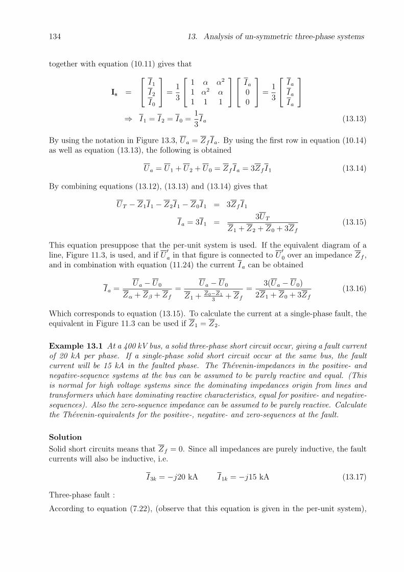
134 13. Analysis of un-symmetric three-phase systems
together with equation (10.11) gives that
Is =
I1
I2
I0
=
1
3
1 α α2
1 α2 α1 1 1
Ia
00
=
1
3
Ia
Ia
Ia
⇒ I1 = I2 = I0 =1
3Ia (13.13)
By using the notation in Figure 13.3, Ua = ZfIa. By using the first row in equation (10.14)as well as equation (13.13), the following is obtained
Ua = U1 + U2 + U0 = ZfIa = 3ZfI1 (13.14)
By combining equations (13.12), (13.13) and (13.14) gives that
UT − Z1I1 − Z2I1 − Z0I1 = 3ZfI1
Ia = 3I1 =3UT
Z1 + Z2 + Z0 + 3Zf
(13.15)
This equation presuppose that the per-unit system is used. If the equivalent diagram of aline, Figure 11.3, is used, and if U
′a in that figure is connected to U
′0 over an impedance Zf ,
and in combination with equation (11.24) the current Ia can be obtained
Ia =Ua − U0
Zα + Zβ + Zf
=Ua − U0
Z1 + Z0−Z1
3+ Zf
=3(Ua − U0)
2Z1 + Z0 + 3Zf
(13.16)
Which corresponds to equation (13.15). To calculate the current at a single-phase fault, theequivalent in Figure 11.3 can be used if Z1 = Z2.
Example 13.1 At a 400 kV bus, a solid three-phase short circuit occur, giving a fault currentof 20 kA per phase. If a single-phase solid short circuit occur at the same bus, the faultcurrent will be 15 kA in the faulted phase. The Thevenin-impedances in the positive- andnegative-sequence systems at the bus can be assumed to be purely reactive and equal. (Thisis normal for high voltage systems since the dominating impedances origin from lines andtransformers which have dominating reactive characteristics, equal for positive- and negative-sequences). Also the zero-sequence impedance can be assumed to be purely reactive. Calculatethe Thevenin-equivalents for the positive-, negative- and zero-sequences at the fault.
Solution
Solid short circuits means that Zf = 0. Since all impedances are purely inductive, the faultcurrents will also be inductive, i.e.
I3k = −j20 kA I1k = −j15 kA (13.17)
Three-phase fault :
According to equation (7.22), (observe that this equation is given in the per-unit system),
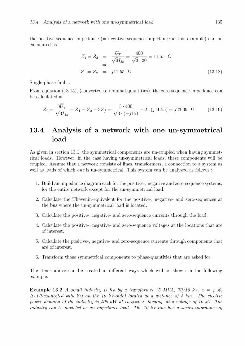
13.4. Analysis of a network with one un-symmetrical load 135
the positive-sequence impedance (= negative-sequence impedance in this example) can becalculated as
Z1 = Z2 =UT√3I3k
=400√3 · 20
= 11.55 Ω
⇒Z1 = Z2 = j11.55 Ω (13.18)
Single-phase fault :
From equation (13.15), (converted to nominal quantities), the zero-sequence impedance canbe calculated as
Z0 =3UT√3I1k
− Z1 − Z2 − 3Zf =3 · 400√
3 · (−j15)− 2 · (j11.55) = j23.09 Ω (13.19)
13.4 Analysis of a network with one un-symmetrical
load
As given in section 13.1, the symmetrical components are un-coupled when having symmet-rical loads. However, in the case having un-symmetrical loads, these components will becoupled. Assume that a network consists of lines, transformers, a connection to a system aswell as loads of which one is un-symmetrical. This system can be analyzed as follows :
1. Build an impedance diagram each for the positive-, negative and zero-sequence systems,for the entire network except for the un-symmetrical load.
2. Calculate the Thevenin-equivalent for the positive-, negative- and zero-sequences atthe bus where the un-symmetrical load is located.
3. Calculate the positive-, negative- and zero-sequence currents through the load.
4. Calculate the positive-, negative- and zero-sequence voltages at the locations that areof interest.
5. Calculate the positive-, negative- and zero-sequence currents through components thatare of interest.
6. Transform those symmetrical components to phase-quantities that are asked for.
The items above can be treated in different ways which will be shown in the followingexample.
Example 13.2 A small industry is fed by a transformer (5 MVA, 70/10 kV, x = 4 %,∆-Y0-connected with Y 0 on the 10 kV-side) located at a distance of 5 km. The electricpower demand of the industry is 400 kW at cosφ=0.8, lagging, at a voltage of 10 kV. Theindustry can be modeled as an impedance load. The 10 kV-line has a series impedance of
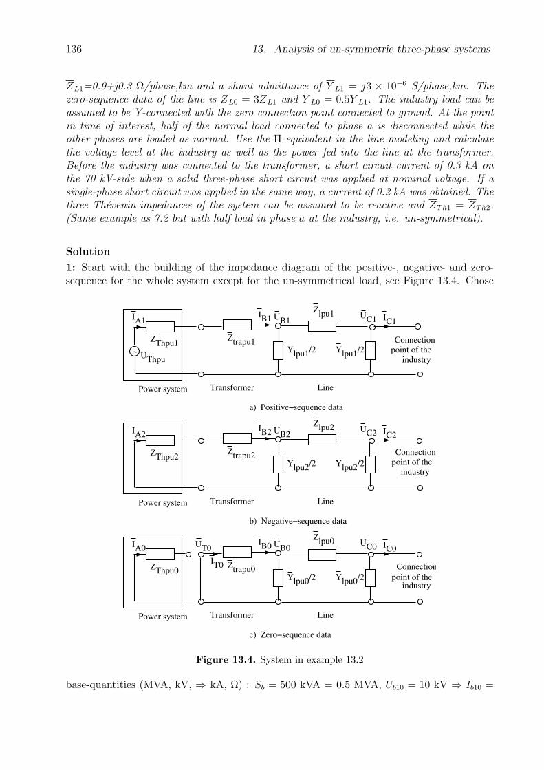
136 13. Analysis of un-symmetric three-phase systems
ZL1=0.9+j0.3 Ω/phase,km and a shunt admittance of Y L1 = j3 × 10−6 S/phase,km. Thezero-sequence data of the line is ZL0 = 3ZL1 and Y L0 = 0.5Y L1. The industry load can beassumed to be Y-connected with the zero connection point connected to ground. At the pointin time of interest, half of the normal load connected to phase a is disconnected while theother phases are loaded as normal. Use the Π-equivalent in the line modeling and calculatethe voltage level at the industry as well as the power fed into the line at the transformer.Before the industry was connected to the transformer, a short circuit current of 0.3 kA onthe 70 kV-side when a solid three-phase short circuit was applied at nominal voltage. If asingle-phase short circuit was applied in the same way, a current of 0.2 kA was obtained. Thethree Thevenin-impedances of the system can be assumed to be reactive and ZTh1 = ZTh2.(Same example as 7.2 but with half load in phase a at the industry, i.e. un-symmetrical).
Solution
1: Start with the building of the impedance diagram of the positive-, negative- and zero-sequence for the whole system except for the un-symmetrical load, see Figure 13.4. Chose
Ylpu1/2Ylpu1/2
Zlpu1
~
Line Transformer
ZThpu1
UThpu
Power system
UB1UC1
Ztrapu1
IC1IB1IA1
a) Positive−sequence data
Connectionpoint of the
industry
Ylpu2/2Ylpu2/2
Zlpu2
Line Transformer
ZThpu2
Power system
UB2UC2
Ztrapu2
IC2IB2IA2
b) Negative−sequence data
Connectionpoint of the
industry
Ylpu0/2Ylpu0/2
Zlpu0
Line Transformer
ZThpu0
Power system
UB0UC0
Ztrapu0
IC0IB0IA0
c) Zero−sequence data
point of theindustry
Connection
UT0
IT0
Figure 13.4. System in example 13.2
base-quantities (MVA, kV, ⇒ kA, Ω) : Sb = 500 kVA = 0.5 MVA, Ub10 = 10 kV ⇒ Ib10 =
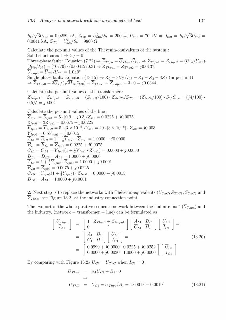
13.4. Analysis of a network with one un-symmetrical load 137
Sb/√
3Ub10 = 0.0289 kA, Zb10 = U2b10/Sb = 200 Ω, Ub70 = 70 kV ⇒ Ib70 = Sb/
√3Ub70 =
0.0041 kA, Zb70 = U2b70/Sb = 9800 Ω
Calculate the per-unit values of the Thevenin-equivalents of the system :Solid short circuit ⇒ Zf = 0Three-phase fault : Equation (7.22)⇒ ZThpu = UThpu/Ikpu ⇒ ZThpu1 = ZThpu2 = (UTh/Ub70)·(Ib70/I3k) = (70/70) · (0.00412/0.3) ⇒ ZThpu1 = ZThpu2 = j0.0137,UThpu = UTh/Ub70 = 1.06 0
Single-phase fault: Equation (13.15) ⇒ Z0 = 3UT /I1k − Z1 − Z2 − 3Zf (in per-unit)⇒ ZThpu0 = 3UT /(
√3I1kZb70)− ZThpu1 − ZThpu2 − 3 · 0 = j0.0344
Calculate the per-unit values of the transformer :Ztrapu1 = Ztrapu2 = Ztrapu0 = (Ztra%/100) · Zbtra70/Zb70 = (Ztra%/100) · Sb/Stra = (j4/100) ·0.5/5 = j0.004
Calculate the per-unit values of the line :Z lpu1 = Z lpu1 = 5 · [0.9 + j0.3]/Zb10 = 0.0225 + j0.0075Z lpu0 = 3Z lpu1 = 0.0675 + j0.0225Y lpu1 = Y lpu2 = 5 · [3× 10−6]/Yb10 = 20 · [3× 10−6] · Zb10 = j0.003Y lpu0 = 0.5Y lpu1 = j0.0015AL1 = AL2 = 1 + 1
2Y lpu1 · Z lpu1 = 1.0000 + j0.0000
BL1 = BL2 = Z lpu1 = 0.0225 + j0.0075CL1 = CL2 = Y lpu1(1 + 1
4Y lpu1 · Z lpu1) = 0.0000 + j0.0030
DL1 = DL2 = AL1 = 1.0000 + j0.0000AL0 = 1 + 1
2Y lpu0 · Z lpu0 = 1.0000 + j0.0001
BL0 = Z lpu0 = 0.0675 + j0.0225CL0 = Y lpu0(1 + 1
4Y lpu0) · Z lpu0 = 0.0000 + j0.0015
DL0 = AL1 = 1.0000 + j0.0001
2: Next step is to replace the networks with Thevenin-equivalents (UThC , ZThC1, ZThC2 andZThC0, see Figure 13.2) at the industry connection point.
The twoport of the whole positive-sequence network between the “infinite bus” (UThpu) andthe industry, (network + transformer + line) can be formulated as
[UThpu
IA1
]=
[1 ZThpu1 + Ztrapu1
0 1
] [AL1 BL1
CL1 DL1
] [UC1
IC1
]=
=
[A1 B1
C1 D1
] [UC1
IC1
]= (13.20)
=
[0.9999 + j0.0000 0.0225 + j0.02520.0000 + j0.0030 1.0000 + j0.0000
] [UC1
IC1
]
By comparing with Figure 13.2a UC1 = UThC when IC1 = 0 :
UThpu = A1UC1 + B1 · 0⇒
UThC = UC1 = UThpu/A1 = 1.0001 6 − 0.0019 (13.21)

138 13. Analysis of un-symmetric three-phase systems
The Thevenin-impedance ZThC1 is calculated as the quotient −UC1/IC1 when UThpu = 0 :
0 = A1UC1 + B1IC1
⇒ZThC1 = −UC1/IC1 = B1/A1 = 0.0225 + j0.0252 (13.22)
The Thevenin-impedance of the negative-sequence at the industry connection point is thesame as for the positive-sequence since the only difference between the impedance networksis the voltage source UThpu : ZThC2 = ZThC1 = 0.0225 + j0.0252
According to Figure 12.2c, the zero-sequence of a ∆-Y0-transformer should be modeled asan impedance to ground on the Y 0-side, as shown in Figure 13.4c. As seen in the figure,the feeding network is not connected to the industry load from a zero-sequence point ofview, owing to this transformer. The twoport of the network from the transformer to theconnection point of the industry (transformer + line) can be given as
[UT0
IT0
]=
[0
IT0
]=
[1 Ztrapu1
0 1
] [AL0 BL0
CL0 DL0
] [UC0
IC0
]=
=
[A0 B0
C0 D0
] [UC0
IC0
]=
=
[1.0000 + j0.0001 0.0675 + j0.02650.0000 + j0.0015 1.0000 + j0.0001
] [UC0
IC0
](13.23)
The Thevenin-impedance ZThC0 can be calculated as the quotient −UC0/IC0 since UT0 = 0 :
0 = A0UC0 + B0IC0
⇒ZThC0 = −UC0/IC0 = B0/A0 = 0.0675 + j0.0265 (13.24)
3: Calculate the per-unit values of the industry impedance in normal conditions :
Zindpu = (U2
ind/S∗ind)/Zb10 = (102/[0.4/0.8]) · (0.8 + j0.6)/200 = 0.8 + j0.6 (13.25)
At half load in phase a (Za = 2Zindpu), the impedance matrix of the symmetrical componentscan be calculated according to equation (13.3) :
Zlds = T−1ZfT = T−1
2Zindpu 0 00 Zindpu 00 0 Zindpu
T (13.26)
=
1.0667 + j0.8000 0.2667 + j0.2000 0.2667 + j0.20000.2667 + j0.2000 1.0667 + j0.8000 0.2667 + j0.20000.2667 + j0.2000 0.2667 + j0.2000 1.0667 + j0.8000
The equation of the whole system can be formed as :
UTh =
UThC
00
= (Zs + Zlds)Is (13.27)
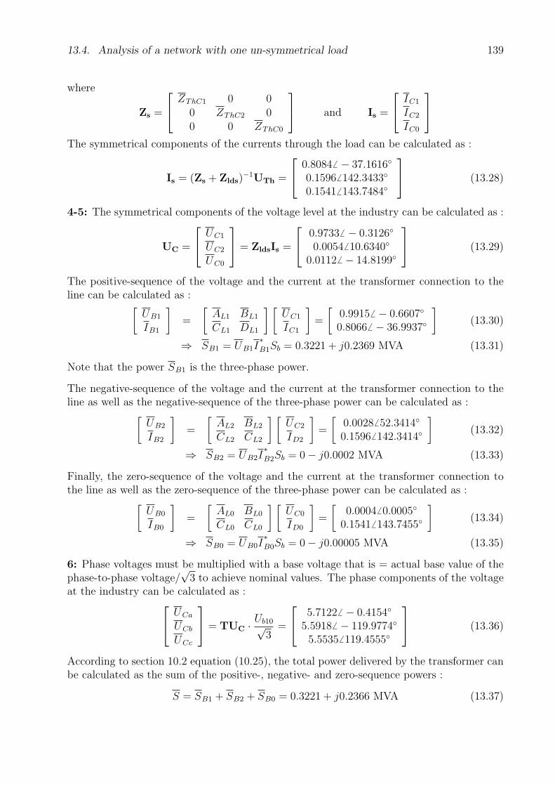
13.4. Analysis of a network with one un-symmetrical load 139
where
Zs =
ZThC1 0 00 ZThC2 00 0 ZThC0
and Is =
IC1
IC2
IC0
The symmetrical components of the currents through the load can be calculated as :
Is = (Zs + Zlds)−1UTh =
0.8084 6 − 37.1616
0.15966 142.3433
0.15416 143.7484
(13.28)
4-5: The symmetrical components of the voltage level at the industry can be calculated as :
UC =
UC1
UC2
UC0
= ZldsIs =
0.97336 − 0.3126
0.00546 10.6340
0.0112 6 − 14.8199
(13.29)
The positive-sequence of the voltage and the current at the transformer connection to theline can be calculated as :
[UB1
IB1
]=
[AL1 BL1
CL1 DL1
] [UC1
IC1
]=
[0.99156 − 0.6607
0.8066 6 − 36.9937
](13.30)
⇒ SB1 = UB1I∗B1Sb = 0.3221 + j0.2369 MVA (13.31)
Note that the power SB1 is the three-phase power.
The negative-sequence of the voltage and the current at the transformer connection to theline as well as the negative-sequence of the three-phase power can be calculated as :
[UB2
IB2
]=
[AL2 BL2
CL2 CL2
] [UC2
ID2
]=
[0.0028 6 52.3414
0.15966 142.3414
](13.32)
⇒ SB2 = UB2I∗B2Sb = 0− j0.0002 MVA (13.33)
Finally, the zero-sequence of the voltage and the current at the transformer connection tothe line as well as the zero-sequence of the three-phase power can be calculated as :
[UB0
IB0
]=
[AL0 BL0
CL0 CL0
] [UC0
ID0
]=
[0.00046 0.0005
0.15416 143.7455
](13.34)
⇒ SB0 = UB0I∗B0Sb = 0− j0.00005 MVA (13.35)
6: Phase voltages must be multiplied with a base voltage that is = actual base value of thephase-to-phase voltage/
√3 to achieve nominal values. The phase components of the voltage
at the industry can be calculated as :
UCa
UCb
UCc
= TUC · Ub10√
3=
5.7122 6 − 0.4154
5.5918 6 − 119.9774
5.55356 119.4555
(13.36)
According to section 10.2 equation (10.25), the total power delivered by the transformer canbe calculated as the sum of the positive-, negative- and zero-sequence powers :
S = SB1 + SB2 + SB0 = 0.3221 + j0.2366 MVA (13.37)
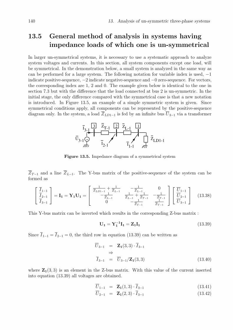
140 13. Analysis of un-symmetric three-phase systems
13.5 General method of analysis in systems having
impedance loads of which one is un-symmetrical
In larger un-symmetrical systems, it is necessary to use a systematic approach to analyzesystem voltages and currents. In this section, all system components except one load, willbe symmetrical. In the demonstration below, a small system is analyzed in the same way ascan be performed for a large system. The following notation for variable index is used, −1indicate positive-sequence, −2 indicate negative-sequence and −0 zero-sequence. For vectors,the corresponding index are 1, 2 and 0. The example given below is identical to the one insection 7.3 but with the difference that the load connected at bus 2 is un-symmetric. In theinitial stage, the only difference compared with the symmetrical case is that a new notationis introduced. In Figure 13.5, an example of a simple symmetric system is given. Sincesymmetrical conditions apply, all components can be represented by the positive-sequencediagram only. In the system, a load ZLD1−1 is fed by an infinite bus U3−1 via a transformer
~
2 13
ZLD11
ZL1
ZT1
U31
I21 I
11
I31
Figure 13.5. Impedance diagram of a symmetrical system
ZT−1 and a line ZL−1. The Y-bus matrix of the positive-sequence of the system can beformed as
I1−1
I2−1
I3−1
= I1 = Y1U1 =
1ZLD1−1
+ 1ZL−1
− 1ZL−1
0
− 1ZL−1
1ZL−1
+ 1ZT−1
− 1ZT−1
0 − 1ZT−1
1ZT−1
U1−1
U2−1
U3−1
(13.38)
This Y-bus matrix can be inverted which results in the corresponding Z-bus matrix :
U1 = Y−11 I1 = Z1I1 (13.39)
Since I1−1 = I2−1 = 0, the third row in equation (13.39) can be written as
U3−1 = Z1(3, 3) · I3−1
⇒I3−1 = U3−1/Z1(3, 3) (13.40)
where Z1(3, 3) is an element in the Z-bus matrix. With this value of the current insertedinto equation (13.39) all voltages are obtained.
U1−1 = Z1(1, 3) · I3−1 (13.41)
U2−1 = Z1(2, 3) · I3−1 (13.42)

13.5. General method of analysis in systems havingimpedance loads of which one is un-symmetrical 141
So far, all calculations are identical to those in section 7.3. Corresponding calculations canbe performed for an arbitrary large system having impedance loads and one voltage source.Assume a system with a voltage source at bus i. The current at bus i and the voltage atanother bus r can then be calculated as
I i−1 = U i−1/Z1(i, i) (13.43)
U r−1 = Z1(r, i) · I i−1 (13.44)
Assume that an un-symmetric impedance load is added to the system at bus 2. The systemvoltages and currents will then be changed in the whole system. The new voltages can beobtained by using the theorem of superposition, i.e. as the sum of the voltages before theconnection of the load and with the voltage change obtained by the load connection. Thiscan be expressed by using symmetrical components as :
U′1 = U1 + U∆1
U′2 = U2 + U∆2 (13.45)
U′0 = U0 + U∆0
where
U′1 = vector of positive-sequence voltages at all buses after the connection of the un-symmetrical
load
U′2 = vector of negative-sequence voltages at all buses after the connection of the un-
symmetrical load
U′0 = vector of zero-sequence voltages at all buses after the connection of the un-symmetrical
load
U1 = vector of positive-sequence voltages at all buses prior to the connection of the un-symmetrical load, same vector as above
U2 = vector of negative-sequence voltages at all buses prior to the connection of the un-symmetrical load. This vector is here ≡ 0 since the conditions are symmetric prior tothe connection of the un-symmetrical load
U0 = vector of zero-sequence voltages at all buses prior to the connection of the un-symmetricalload. This vector is here ≡ 0 since the conditions are symmetric prior to the connectionof the un-symmetrical load
U∆1 = vector of changes in the positive-sequence voltages at all buses caused by the con-nection of the un-symmetrical load
U∆2 = vector of changes in the negative-sequence voltages at all buses caused by the con-nection of the un-symmetrical load
U∆0 = vector of changes in the zero-sequence voltages caused by the connection of theun-symmetrical load
142 13. Analysis of un-symmetric three-phase systems
Equation (13.45) can be rewritten by expressing the voltage changes by a Z-bus matrixmultiplied with the current changes injected at the buses.
U′1 = U1 + Z∆1I∆1
U′2 = 0 + Z∆2I∆2 (13.46)
U′0 = 0 + Z∆0I∆0
where
Z∆1 = Z-bus matrix of the positive-sequence data with voltage sources shortened
Z∆2 = Z-bus matrix of the negative-sequence data
Z∆0 = Z-bus matrix of the zero-sequence data
I∆1 = vector of the injected positive-sequence current changes at the buses, only I∆1(2) 6= 0,since the load is connected at that bus
I∆2 = vector of the injected negative-sequence current changes at the buses, only I∆2(2) 6= 0
I∆0 = vector of the injected zero-sequence current changes at the buses, only I∆0(2) 6= 0
In Figure 13.6, the positive-, negative- and zero-sequence systems used in the calculationsof the voltage changes when connecting an un-symmetrical load at any bus are given. Thedifference between the positive-sequence system in Figure 13.6 and the ∆-system used insection 7.3 is that the load is now represented by the currents injected into the buses. Theinfinite bus is assumed to be directly connected to ground and the transformer is Y oY o-connected. The Y-bus matrices of the network given in Figure 13.6 can be formed as
Y∆1 =
[1
ZLD1−1+ 1
ZL−1− 1
ZL−1
− 1ZL−1
1ZL−1
+ 1ZT−1
](13.47)
Y∆2 =
[1
ZLD1−2+ 1
ZL−2− 1
ZL−2
− 1ZL−2
1ZL−2
+ 1ZT−2
](13.48)
Y∆0 =
[1
ZLD1−0+ 1
ZL−0− 1
ZL−0
− 1ZL−0
1ZL−0
+ 1ZT−0
](13.49)
The matrix Y∆1 is the matrix Y1 but the row and column that corresponds to the generatorbus (= bus 1) are cancelled, compare section 7.3. When only having lines, transformers andsymmetrical loads in the system, Y∆2 = Y∆1 since all components have positive-sequencedata that are equal to the negative-sequence data. From these Y-bus matrices the corre-sponding Z-bus matrices can be calculated as
Z∆1 = Y−1∆1 (13.50)
Z∆2 = Y−1∆2 (13.51)
Z∆0 = Y−1∆0 (13.52)
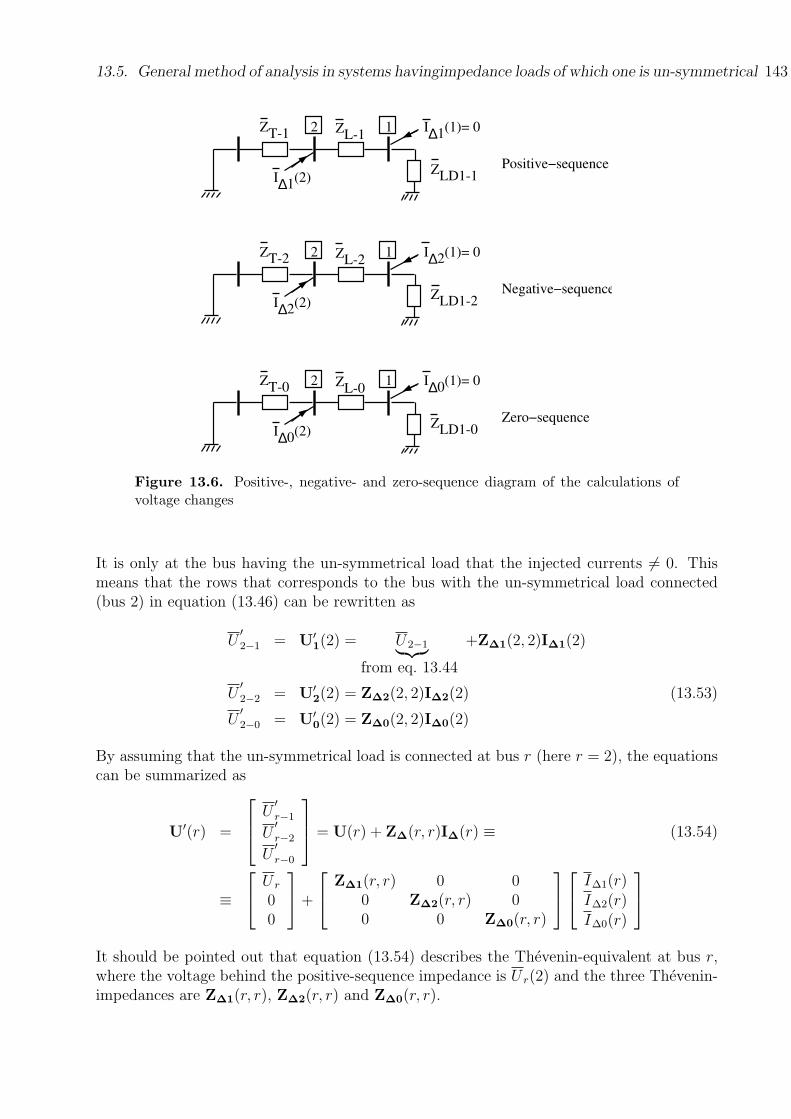
13.5. General method of analysis in systems havingimpedance loads of which one is un-symmetrical 143
2 1
ZLD11
ZL1ZT1
I∆1(2)
I∆1(1)= 0
Positive−sequence
2 1
ZLD12
ZL2ZT2
I∆2(2)
I∆2(1)= 0
Negative−sequence
2 1
ZLD10
ZL0ZT0
I∆0(2)
I∆0(1)= 0
Zero−sequence
Figure 13.6. Positive-, negative- and zero-sequence diagram of the calculations ofvoltage changes
It is only at the bus having the un-symmetrical load that the injected currents 6= 0. Thismeans that the rows that corresponds to the bus with the un-symmetrical load connected(bus 2) in equation (13.46) can be rewritten as
U′2−1 = U′
1(2) = U2−1︸︷︷ ︸from eq. 13.44
+Z∆1(2, 2)I∆1(2)
U′2−2 = U′
2(2) = Z∆2(2, 2)I∆2(2) (13.53)
U′2−0 = U′
0(2) = Z∆0(2, 2)I∆0(2)
By assuming that the un-symmetrical load is connected at bus r (here r = 2), the equationscan be summarized as
U′(r) =
U′r−1
U′r−2
U′r−0
= U(r) + Z∆(r, r)I∆(r) ≡ (13.54)
≡
U r
00
+
Z∆1(r, r) 0 00 Z∆2(r, r) 00 0 Z∆0(r, r)
I∆1(r)I∆2(r)I∆0(r)
It should be pointed out that equation (13.54) describes the Thevenin-equivalent at bus r,where the voltage behind the positive-sequence impedance is U r(2) and the three Thevenin-impedances are Z∆1(r, r), Z∆2(r, r) and Z∆0(r, r).

144 13. Analysis of un-symmetric three-phase systems
Assume that the un-symmetrical load is Y-connected and connected to ground and consistsof three different impedances in the three phases : ZLD2−a, ZLD2−b and ZLD2−c. The voltagedrop (in the phase components) over the load is
ULD2−phase =
ULD2−a
ULD2−b
ULD2−c
=
ZLD2−a 0 00 ZLD2−b 00 0 ZLD2−c
ILD2−a
ILD2−b
ILD2−c
≡
≡ ZLD2−phaseILD2−phase (13.55)
By introducing symmetrical components, this can be converted to
U′(2) =
U′2−1
U′2−2
U′2−0
= T−1ULD2−phase = T−1ZLD2−phaseILD2−phase =
= T−1ZLD2−phaseT︸ ︷︷ ︸=ZLD2−sym
ILD2−sym = −ZLD2−symI∆(2) (13.56)
since the direction of definitions for currents in equation (13.55) is down into the load (=outfrom the bus) whereas I∆(2) has the direction of definitions into the bus.
By assuming that the un-symmetrical load is connected to bus r (here r = 2) the currentI∆(r) can be calculated by summarizing equation (13.54) and (13.56).
I∆(r) = − [Z∆(r, r) + ZLDr−sym]−1 U(r) (13.57)
These values of the symmetrical components of the current at bus r can then be insertedinto equation (13.46) where the symmetrical components of all voltages can be calculated.The voltage at bus k can then be calculated as :
U′1(k) = U1(k) + Z∆1(k, r)I∆1(r)
U′2(k) = Z∆2(k, r)I∆2(r) (13.58)
U′0(k) = Z∆0(k, r)I∆0(r)
Example 13.3 In Figure 13.7, an internal industry network is shown. The electric energyis delivered by an infinite bus 1 having nominal voltage and a grounded zero connection point.The energy is distributed via transformer T1, the line L2 and the transformer T2 to the loadLD2. There is also a high voltage load LD1 connected to T1 via the line L1. Componentdata are :
• Transformer T1 : 800 kVA, 70/10 kV, x = 7 %, Y0-∆ with Y 0 on the 10-kV side
• Transformer T2 : 300 kVA, 0.4/10 kV, x = 8 %, Y 0− Y 0
• Line L1 : rL1−1 = 0.17 Ω/km, ωLL1−1 = 0.3 Ω/km, ωCL1−1 = 3.2 × 10⁻⁶ S/km,` = 2 km, ZL1−0 = 3ZL1−1, Y L1−0 = 0.5Y L1−1,
• Line L2 : rL2−1 = 0.17 Ω/km, ωLL2−1 = 0.3 Ω/km, ωCL2−1 = 3.2 × 10⁻⁶ S/km,` = 1 km, ZL2−0 = 3ZL2−1, Y L2−0 = 0.5Y L2−1,
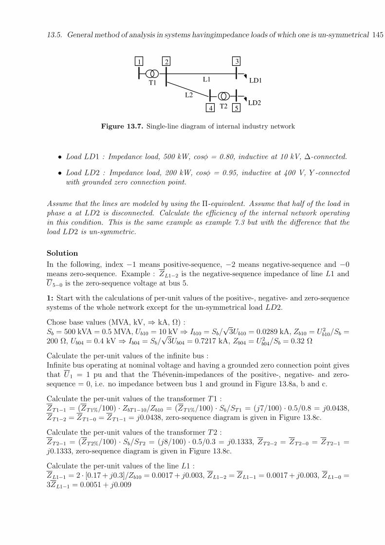
13.5. General method of analysis in systems havingimpedance loads of which one is un-symmetrical 145
1 2 3
54
L1
L2
T1
T2
LD1
LD2
Figure 13.7. Single-line diagram of internal industry network
• Load LD1 : Impedance load, 500 kW, cosφ = 0.80, inductive at 10 kV, ∆-connected.
• Load LD2 : Impedance load, 200 kW, cosφ = 0.95, inductive at 400 V, Y -connectedwith grounded zero connection point.
Assume that the lines are modeled by using the Π-equivalent. Assume that half of the load inphase a at LD2 is disconnected. Calculate the efficiency of the internal network operatingin this condition. This is the same example as example 7.3 but with the difference that theload LD2 is un-symmetric.
Solution
In the following, index −1 means positive-sequence, −2 means negative-sequence and −0means zero-sequence. Example : ZL1−2 is the negative-sequence impedance of line L1 andU5−0 is the zero-sequence voltage at bus 5.
1: Start with the calculations of per-unit values of the positive-, negative- and zero-sequencesystems of the whole network except for the un-symmetrical load LD2.
Chose base values (MVA, kV, ⇒ kA, Ω) :Sb = 500 kVA = 0.5 MVA, Ub10 = 10 kV ⇒ Ib10 = Sb/
√3Ub10 = 0.0289 kA, Zb10 = U2
b10/Sb =200 Ω, Ub04 = 0.4 kV ⇒ Ib04 = Sb/
√3Ub04 = 0.7217 kA, Zb04 = U2
b04/Sb = 0.32 Ω
Calculate the per-unit values of the infinite bus :Infinite bus operating at nominal voltage and having a grounded zero connection point givesthat U1 = 1 pu and that the Thevenin-impedances of the positive-, negative- and zero-sequence = 0, i.e. no impedance between bus 1 and ground in Figure 13.8a, b and c.
Calculate the per-unit values of the transformer T1 :ZT1−1 = (ZT1%/100) · ZbT1−10/Zb10 = (ZT1%/100) · Sb/ST1 = (j7/100) · 0.5/0.8 = j0.0438,ZT1−2 = ZT1−0 = ZT1−1 = j0.0438, zero-sequence diagram is given in Figure 13.8c.
Calculate the per-unit values of the transformer T2 :ZT2−1 = (ZT2%/100) · Sb/ST2 = (j8/100) · 0.5/0.3 = j0.1333, ZT2−2 = ZT2−0 = ZT2−1 =j0.1333, zero-sequence diagram is given in Figure 13.8c.
Calculate the per-unit values of the line L1 :ZL1−1 = 2 · [0.17 + j0.3]/Zb10 = 0.0017 + j0.003, ZL1−2 = ZL1−1 = 0.0017 + j0.003, ZL1−0 =3ZL1−1 = 0.0051 + j0.009
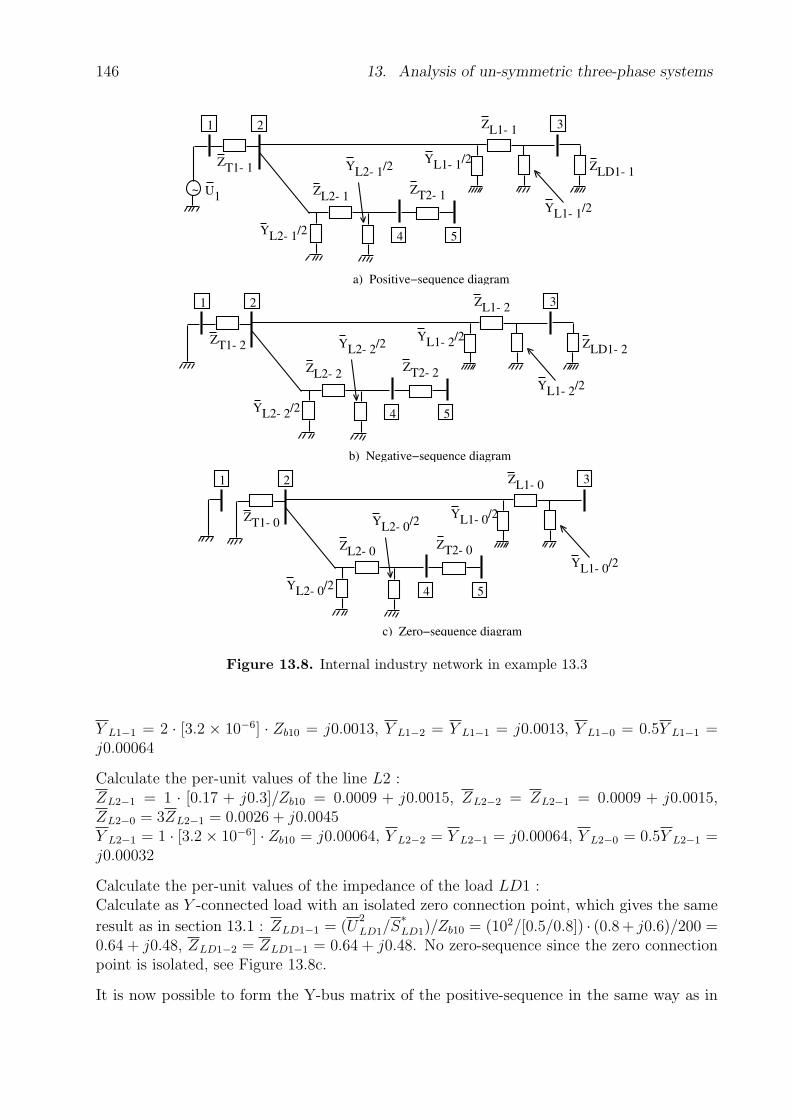
146 13. Analysis of un-symmetric three-phase systems
1 2 3
54
ZL1 1
ZT1 1YL1 1/2
ZL2 1
YL2 1/2
ZT2 1
ZLD1 1
YL1 1/2
YL2 1/2
a) Positive−sequence diagram
~ U1
1 2 3
54
ZL1 2
ZT1 2YL1 2/2
ZL2 2
YL2 2/2
ZT2 2
ZLD1 2
YL1 2/2
YL2 2/2
b) Negative−sequence diagram
1 2 3
54
ZL1 0
ZT1 0YL1 0/2
ZL2 0
YL2 0/2
ZT2 0YL1 0/2
YL2 0/2
c) Zero−sequence diagram
Figure 13.8. Internal industry network in example 13.3
Y L1−1 = 2 · [3.2 × 10−6] · Zb10 = j0.0013, Y L1−2 = Y L1−1 = j0.0013, Y L1−0 = 0.5Y L1−1 =j0.00064
Calculate the per-unit values of the line L2 :ZL2−1 = 1 · [0.17 + j0.3]/Zb10 = 0.0009 + j0.0015, ZL2−2 = ZL2−1 = 0.0009 + j0.0015,ZL2−0 = 3ZL2−1 = 0.0026 + j0.0045Y L2−1 = 1 · [3.2× 10−6] · Zb10 = j0.00064, Y L2−2 = Y L2−1 = j0.00064, Y L2−0 = 0.5Y L2−1 =j0.00032
Calculate the per-unit values of the impedance of the load LD1 :Calculate as Y -connected load with an isolated zero connection point, which gives the same
result as in section 13.1 : ZLD1−1 = (U2
LD1/S∗LD1)/Zb10 = (102/[0.5/0.8]) · (0.8 + j0.6)/200 =
0.64 + j0.48, ZLD1−2 = ZLD1−1 = 0.64 + j0.48. No zero-sequence since the zero connectionpoint is isolated, see Figure 13.8c.
It is now possible to form the Y-bus matrix of the positive-sequence in the same way as in
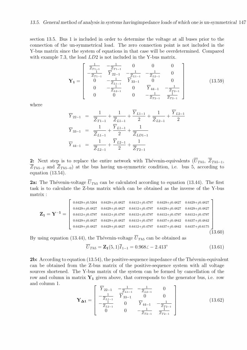
13.5. General method of analysis in systems havingimpedance loads of which one is un-symmetrical 147
section 13.5. Bus 1 is included in order to determine the voltage at all buses prior to theconnection of the un-symmetrical load. The zero connection point is not included in theY-bus matrix since the system of equations in that case will be overdetermined. Comparedwith example 7.3, the load LD2 is not included in the Y-bus matrix.
Y1 =
1ZT1−1
− 1ZT1−1
0 0 0
− 1ZT1−1
Y 22−1 − 1ZL1−1
− 1ZL2−1
0
0 − 1ZL1−1
Y 33−1 0 0
0 − 1ZL2−1
0 Y 44−1 − 1ZT2−1
0 0 0 − 1ZT2−1
1ZT2−1
(13.59)
where
Y 22−1 =1
ZT1−1
+1
ZL1−1
+Y L1−1
2+
1
ZL2−1
+Y L2−1
2
Y 33−1 =1
ZL1−1
+Y L1−1
2+
1
ZLD1−1
Y 44−1 =1
ZL2−1
+Y L2−1
2+
1
ZT2−1
2: Next step is to replace the entire network with Thevenin-equivalents (UTh5, ZTh5−1,ZTh5−2 and ZTh5−0) at the bus having un-symmetric condition, i.e. bus 5, according toequation (13.54).
2a: The Thevenin-voltage UTh5 can be calculated according to equation (13.44). The firsttask is to calculate the Z-bus matrix which can be obtained as the inverse of the Y-busmatrix :
Z1 = Y−1 =
0.6429+j0.5264 0.6429+j0.4827 0.6412+j0.4797 0.6429+j0.4827 0.6429+j0.4827
0.6429+j0.4827 0.6429+j0.4827 0.6412+j0.4797 0.6429+j0.4827 0.6429+j0.4827
0.6412+j0.4797 0.6412+j0.4797 0.6412+j0.4797 0.6412+j0.4797 0.6412+j0.4797
0.6429+j0.4827 0.6429+j0.4827 0.6412+j0.4797 0.6437+j0.4842 0.6437+j0.4842
0.6429+j0.4827 0.6429+j0.4827 0.6412+j0.4797 0.6437+j0.4842 0.6437+j0.6175
(13.60)By using equation (13.44), the Thevenin-voltage UTh5 can be obtained as
UTh5 = Z1(5, 1)I1−1 = 0.968 6 − 2.413 (13.61)
2b: According to equation (13.54), the positive-sequence impedance of the Thevenin-equivalentcan be obtained from the Z-bus matrix of the positive-sequence system with all voltagesources shortened. The Y-bus matrix of the system can be formed by cancellation of therow and column in matrix Y1 given above, that corresponds to the generator bus, i.e. rowand column 1.
Y∆1 =
Y 22−1 − 1ZL1−1
− 1ZL2−1
0
− 1ZL1−1
Y 33−1 0 0
− 1ZL2−1
0 Y 44−1 − 1ZT2−1
0 0 − 1ZT2−1
1ZT2−1
(13.62)
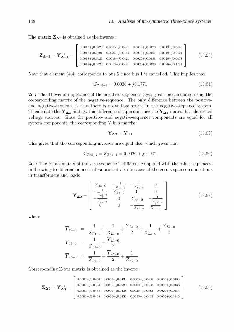
148 13. Analysis of un-symmetric three-phase systems
The matrix Z∆1 is obtained as the inverse :
Z∆−1 = Y−1∆−1 =
0.0018+j0.0423 0.0018+j0.0421 0.0018+j0.0423 0.0018+j0.0423
0.0018+j0.0421 0.0036+j0.0449 0.0018+j0.0421 0.0018+j0.0421
0.0018+j0.0423 0.0018+j0.0421 0.0026+j0.0438 0.0026+j0.0438
0.0018+j0.0423 0.0018+j0.0421 0.0026+j0.0438 0.0026+j0.1771
(13.63)
Note that element (4,4) corresponds to bus 5 since bus 1 is cancelled. This implies that
ZTh5−1 = 0.0026 + j0.1771 (13.64)
2c : The Thevenin-impedance of the negative-sequences ZTh5−2 can be calculated using thecorresponding matrix of the negative-sequence. The only difference between the positive-and negative-sequence is that there is no voltage source in the negative-sequence system.To calculate the Y∆2-matrix, this difference disappears since the Y∆1-matrix has shortenedvoltage sources. Since the positive- and negative-sequence components are equal for allsystem components, the corresponding Y-bus matrix :
Y∆2 = Y∆1 (13.65)
This gives that the corresponding inverses are equal also, which gives that
ZTh5−2 = ZTh5−1 = 0.0026 + j0.1771 (13.66)
2d : The Y-bus matrix of the zero-sequence is different compared with the other sequences,both owing to different numerical values but also because of the zero-sequence connectionsin transformers and loads.
Y∆0 =
Y 22−0 − 1ZL1−0
− 1ZL2−0
0
− 1ZL1−0
Y 33−0 0 0
− 1ZL2−0
0 Y 44−0 − 1ZT2−0
0 0 − 1ZT2−0
1ZT2−0
(13.67)
where
Y 22−0 =1
ZT1−0
+1
ZL1−0
+Y L1−0
2+
1
ZL2−0
+Y L2−0
2
Y 33−0 =1
ZL1−0
+Y L1−0
2
Y 44−0 =1
ZL2−0
+Y L2−0
2+
1
ZT2−0
Corresponding Z-bus matrix is obtained as the inverse
Z∆0 = Y−1∆0 =
0.0000+j0.0438 0.0000+j0.0438 0.0000+j0.0438 0.0000+j0.0438
0.0000+j0.0438 0.0051+j0.0528 0.0000+j0.0438 0.0000+j0.0438
0.0000+j0.0438 0.0000+j0.0438 0.0026+j0.0483 0.0026+j0.0483
0.0000+j0.0438 0.0000+j0.0438 0.0026+j0.0483 0.0026+j0.1816
(13.68)

13.5. General method of analysis in systems havingimpedance loads of which one is un-symmetrical 149
Note that element (4,4) corresponds to bus 5 since bus 1 is cancelled. This gives that
ZTh5−0 = 0.0026 + j0.1816 (13.69)
By that, all Thevenin-quantities of bus 5 are calculated and the voltage vector and impedancematrix according to equation (13.54) are calculated as
U(5) =
UTh5
00
=
0.9686 − 2.413
00
Z∆(5, 5) =
ZTh5−1 0 00 ZTh5−2 00 0 ZTh5−0
= (13.70)
=
0.0026 + j0.1771 0 00 0.0026 + j0.1771 00 0 0.0026 + j0.1816
3: Calculate the per-unit values of the impedance of LD2 in normal conditions :
ZLD2pu = (U2LD2/S
∗LD2)/Zb04 = (13.71)
= (0.42/[0.2/0.95]) · (0.95 + j√
1− 0.952)/0.32 = 2.2562 + j0.7416
At half load in phase a (Za = 2ZLD2), the impedance matrix of the symmetrical componentscan be calculated by using equation (13.3) :
ZLD2−sym = T−1ZLD2−phaseT = T−1
2ZLD2pu 0 00 ZLD2pu 00 0 ZLD2pu
T =
=
3.0083 + j0.9888 0.7521 + j0.2472 0.7521 + j0.24720.7521 + j0.2472 3.0083 + j0.9888 0.7521 + j0.24720.7521 + j0.2472 0.7521 + j0.2472 3.0083 + j0.9888
(13.72)
The symmetrical components of the currents through the load can be calculated by usingequation (13.57) together with data from equation (13.70)
I∆(5) = − [Z∆(5, 5) + ZLDr−sym]−1 U(5) =
0.3315 6 155.8442
0.0653 6 − 26.5244
0.0653 6 − 26.6221
(13.73)
4: The symmetrical components of all voltages can be calculated by using equation (13.58)
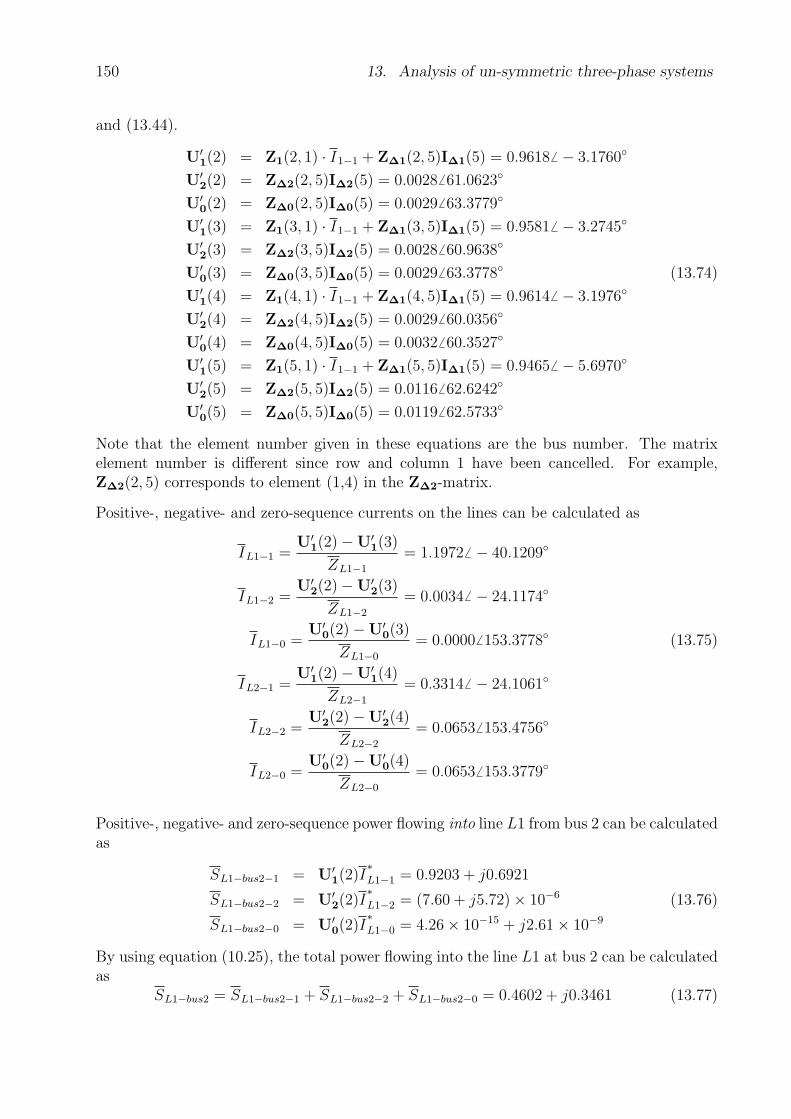
150 13. Analysis of un-symmetric three-phase systems
and (13.44).
U′1(2) = Z1(2, 1) · I1−1 + Z∆1(2, 5)I∆1(5) = 0.96186 − 3.1760
U′2(2) = Z∆2(2, 5)I∆2(5) = 0.00286 61.0623
U′0(2) = Z∆0(2, 5)I∆0(5) = 0.00296 63.3779
U′1(3) = Z1(3, 1) · I1−1 + Z∆1(3, 5)I∆1(5) = 0.95816 − 3.2745
U′2(3) = Z∆2(3, 5)I∆2(5) = 0.00286 60.9638
U′0(3) = Z∆0(3, 5)I∆0(5) = 0.00296 63.3778 (13.74)
U′1(4) = Z1(4, 1) · I1−1 + Z∆1(4, 5)I∆1(5) = 0.96146 − 3.1976
U′2(4) = Z∆2(4, 5)I∆2(5) = 0.00296 60.0356
U′0(4) = Z∆0(4, 5)I∆0(5) = 0.00326 60.3527
U′1(5) = Z1(5, 1) · I1−1 + Z∆1(5, 5)I∆1(5) = 0.94656 − 5.6970
U′2(5) = Z∆2(5, 5)I∆2(5) = 0.01166 62.6242
U′0(5) = Z∆0(5, 5)I∆0(5) = 0.01196 62.5733
Note that the element number given in these equations are the bus number. The matrixelement number is different since row and column 1 have been cancelled. For example,Z∆2(2, 5) corresponds to element (1,4) in the Z∆2-matrix.
Positive-, negative- and zero-sequence currents on the lines can be calculated as
IL1−1 =U′
1(2)−U′1(3)
ZL1−1
= 1.1972 6 − 40.1209
IL1−2 =U′
2(2)−U′2(3)
ZL1−2
= 0.0034 6 − 24.1174
IL1−0 =U′
0(2)−U′0(3)
ZL1−0
= 0.00006 153.3778 (13.75)
IL2−1 =U′
1(2)−U′1(4)
ZL2−1
= 0.3314 6 − 24.1061
IL2−2 =U′
2(2)−U′2(4)
ZL2−2
= 0.06536 153.4756
IL2−0 =U′
0(2)−U′0(4)
ZL2−0
= 0.06536 153.3779
Positive-, negative- and zero-sequence power flowing into line L1 from bus 2 can be calculatedas
SL1−bus2−1 = U′1(2)I
∗L1−1 = 0.9203 + j0.6921
SL1−bus2−2 = U′2(2)I
∗L1−2 = (7.60 + j5.72)× 10−6 (13.76)
SL1−bus2−0 = U′0(2)I
∗L1−0 = 4.26× 10⁻¹⁵ + j2.61× 10−9
By using equation (10.25), the total power flowing into the line L1 at bus 2 can be calculatedas
SL1−bus2 = SL1−bus2−1 + SL1−bus2−2 + SL1−bus2−0 = 0.4602 + j0.3461 (13.77)
13.5. General method of analysis in systems havingimpedance loads of which one is un-symmetrical 151
In the corresponding manner, the total power out from the line L1 at bus 3, as well as thepower in and out from the line L2 can be calculated as
SL1−bus3 = 0.4589 + j0.3461
SL2−bus2 = 0.1489 + j0.0567 (13.78)
SL2−bus4 = 0.1488 + j0.0567
The only system losses are the line losses. These losses can be calculated as the differencebetween the sending and the receiving end power. The efficiency can be calculated as :
η = 100 · Real(SL1−bus3) + Real(SL2−bus4)
Real(SL1−bus2) + Real(SL2−bus2)= 99.7911% (13.79)
152 13. Analysis of un-symmetric three-phase systems
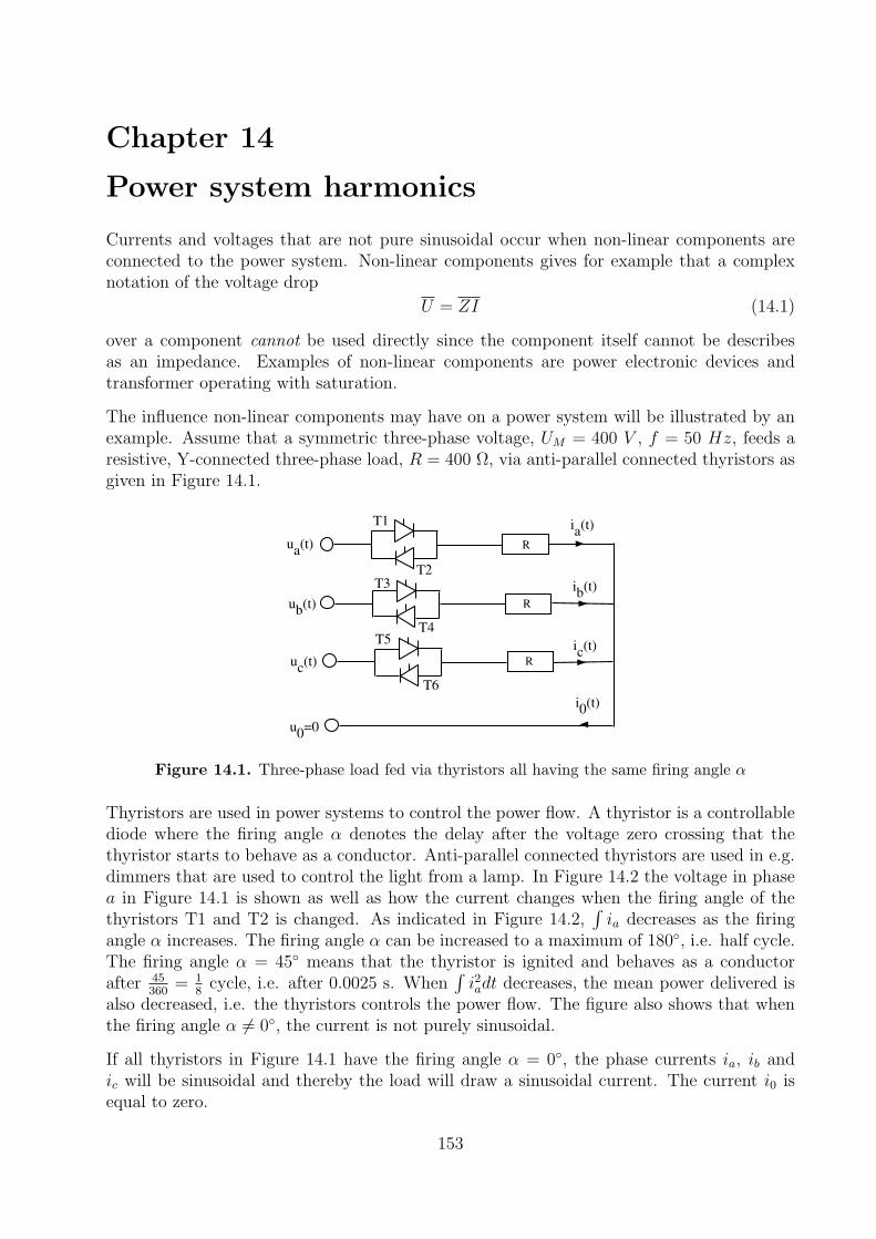
Chapter 14
Power system harmonics
Currents and voltages that are not pure sinusoidal occur when non-linear components areconnected to the power system. Non-linear components gives for example that a complexnotation of the voltage drop
U = ZI (14.1)
over a component cannot be used directly since the component itself cannot be describesas an impedance. Examples of non-linear components are power electronic devices andtransformer operating with saturation.
The influence non-linear components may have on a power system will be illustrated by anexample. Assume that a symmetric three-phase voltage, UM = 400 V , f = 50 Hz, feeds aresistive, Y-connected three-phase load, R = 400 Ω, via anti-parallel connected thyristors asgiven in Figure 14.1.
ua(t)
ub
(t)
uc(t)
ia(t)
ib
(t)
ic(t)
i0
(t)
u0
=0
T1
T4
T2T3
T6
R
R
R
T5
Figure 14.1. Three-phase load fed via thyristors all having the same firing angle α
Thyristors are used in power systems to control the power flow. A thyristor is a controllablediode where the firing angle α denotes the delay after the voltage zero crossing that thethyristor starts to behave as a conductor. Anti-parallel connected thyristors are used in e.g.dimmers that are used to control the light from a lamp. In Figure 14.2 the voltage in phasea in Figure 14.1 is shown as well as how the current changes when the firing angle of thethyristors T1 and T2 is changed. As indicated in Figure 14.2,
∫ia decreases as the firing
angle α increases. The firing angle α can be increased to a maximum of 180, i.e. half cycle.The firing angle α = 45 means that the thyristor is ignited and behaves as a conductorafter 45
360= 1
8cycle, i.e. after 0.0025 s. When
∫i2adt decreases, the mean power delivered is
also decreased, i.e. the thyristors controls the power flow. The figure also shows that whenthe firing angle α 6= 0, the current is not purely sinusoidal.
If all thyristors in Figure 14.1 have the firing angle α = 0, the phase currents ia, ib andic will be sinusoidal and thereby the load will draw a sinusoidal current. The current i0 isequal to zero.
153

154 14. Power system harmonics
Assume that all thyristors instead have a firing angle of 45. The three phase currents aswell as the current in the neutral will have the shape shown in Figure 14.3.
As given in Figure 14.3, the occurrence of thyristors gives a current in the neutral conductor.If the firing angle increases in the circuit, Figure 14.1, the shape of the currents will alsochange. In Figure 14.4 the currents when having a firing angle of 135 at all thyristors areshown.
0 0.005 0.01 0.015 0.02 0.025 0.03 0.035 0.04-500
0
500
ua
0 0.005 0.01 0.015 0.02 0.025 0.03 0.035 0.04-1
0
1
ia_0
0 0.005 0.01 0.015 0.02 0.025 0.03 0.035 0.04-1
0
1
ia_4
5
0 0.005 0.01 0.015 0.02 0.025 0.03 0.035 0.04-1
0
1
ia_1
35
Figure 14.2. The voltage ua(t) and the current ia at a firing angle of 0, 45 and135, respectively, of the thyristors T1 and T2
0 0.005 0.01 0.015 0.02 0.025 0.03 0.035 0.04-1
0
1T1
T2
T1
T2ia(t
)
0 0.005 0.01 0.015 0.02 0.025 0.03 0.035 0.04-1
0
1
T4
T3 T3
ib(t
)
T4
0 0.005 0.01 0.015 0.02 0.025 0.03 0.035 0.04-1
0
1
T6
T5
T6
T5
ic(t
)
0 0.005 0.01 0.015 0.02 0.025 0.03 0.035 0.04-1
0
1
i0(t
)
Figure 14.3. Currents in the circuit given in figure 14.1 when the firing angle is 45
In the analysis of not purely sinusoidal quantities in the power system, Fourier analysis isoften used. The quantity of interest is then studied as the sum of sinusoidal quantities with
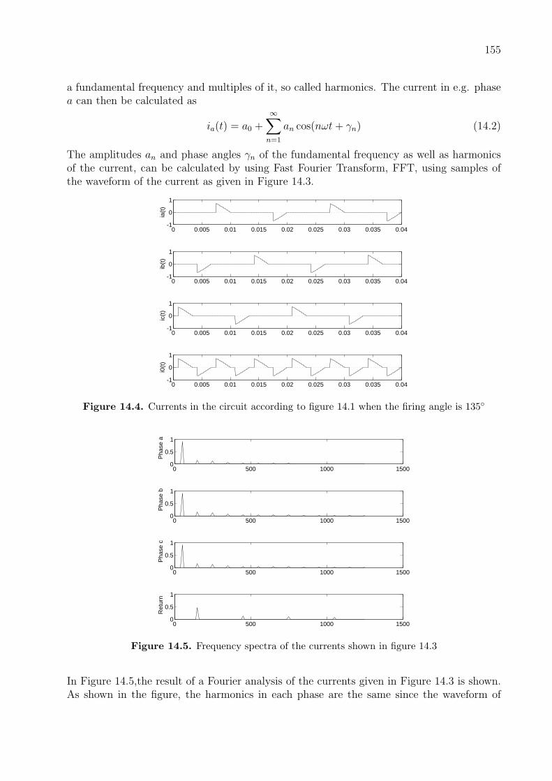
155
a fundamental frequency and multiples of it, so called harmonics. The current in e.g. phasea can then be calculated as
ia(t) = a0 +∞∑
n=1
an cos(nωt + γn) (14.2)
The amplitudes an and phase angles γn of the fundamental frequency as well as harmonicsof the current, can be calculated by using Fast Fourier Transform, FFT, using samples ofthe waveform of the current as given in Figure 14.3.
0 0.005 0.01 0.015 0.02 0.025 0.03 0.035 0.04-1
0
1
ia(t
)
0 0.005 0.01 0.015 0.02 0.025 0.03 0.035 0.04-1
0
1
ib(t
)
0 0.005 0.01 0.015 0.02 0.025 0.03 0.035 0.04-1
0
1
ic(t
)
0 0.005 0.01 0.015 0.02 0.025 0.03 0.035 0.04-1
0
1
i0(t
)
Figure 14.4. Currents in the circuit according to figure 14.1 when the firing angle is 135
0 500 1000 15000
0.5
1
Pha
se a
0 500 1000 15000
0.5
1
Pha
se b
0 500 1000 15000
0.5
1
Pha
se c
0 500 1000 15000
0.5
1
Ret
urn
Figure 14.5. Frequency spectra of the currents shown in figure 14.3
In Figure 14.5,the result of a Fourier analysis of the currents given in Figure 14.3 is shown.As shown in the figure, the harmonics in each phase are the same since the waveform of

156 14. Power system harmonics
the currents are the same in the three phases. For the current i0, the rate of harmonics isdifferent. The rate of harmonics is also given in Table 14.1 which also includes an analysisof the system condition at a firing angle of 135.
α = 45 α = 135
ia i0 ia i0Order Hz A % of 50 Hz A % of 50 Hz A % of 50 Hz A % of 50 Hz
1 50 0.921 100.0 0.004 0.9 0.187 100.0 0.004 0.92 100 0.000 0.0 0.000 0.0 0.000 0.0 0.000 0.03 150 0.162 17.6 0.480 100.0 0.162 86.6 0.480 100.04 200 0.000 0.0 0.000 0.0 0.000 0.0 0.000 0.05 250 0.120 13.0 0.004 0.8 0.120 64.2 0.004 0.86 300 0.000 0.0 0.000 0.0 0.000 0.0 0.000 0.07 350 0.075 8.1 0.004 0.9 0.075 40.2 0.004 0.98 400 0.000 0.0 0.000 0.0 0.000 0.0 0.000 0.09 450 0.045 4.9 0.135 28.1 0.045 24.1 0.135 28.110 500 0.000 0.0 0.000 0.0 0.000 0.0 0.000 0.011 550 0.039 4.2 0.004 0.8 0.039 20.9 0.004 0.812 600 0.000 0.0 0.000 0.0 0.000 0.0 0.000 0.013 650 0.038 4.2 0.004 0.9 0.038 20.6 0.004 0.914 700 0.000 0.0 0.000 0.0 0.000 0.0 0.000 0.015 750 0.032 3.5 0.096 20.1 0.032 17.3 0.096 20.116 800 0.000 0.0 0.000 0.0 0.000 0.0 0.000 0.017 850 0.025 2.7 0.004 0.8 0.025 13.4 0.004 0.818 900 0.000 0.0 0.000 0.0 0.000 0.0 0.000 0.019 950 0.023 2.5 0.004 0.9 0.023 12.4 0.004 0.920 1000 0.000 0.0 0.000 0.0 0.000 0.0 0.000 0.0
THD 100-∞ 0.171 25.4 0.371 100.0 0.171 79.2 0.371 100.0RMS 50-∞ 0.673 100.0 0.371 100.0 0.216 100.0 0.371 100.0
Table 14.1. Harmonics in the phase currents in the circuit given in Figure 14.1 atα = 45 and α = 135
As given in table 14.1, no even harmonics exist. This owing to the anti-parallel connectedthyristors in the three phases that all have the same firing angle giving that the positiveand the negative part of the current have the same waveform, i.e. a mirror image along thetime-axis, see Figure 14.3 and 14.4. In Table 14.1, the Total Harmonic Distortion, THD, isgiven which is an RMS-value of the total harmonics.
THD =
√√√√1
2
∞∑n=2
a2n (14.3)
As given in Table 14.1, the harmonics in the neutral conductor is (mainly) the odd multiplesof three times the fundamental frequency, i.e. 3, 9, 15, etc. (The low percentage levelsgiven for other harmonics in the table are due to limitations in the calculation routine used.)Also the amplitude of the harmonics are higher in the neutral conductor compared with thephase conductors. The reason for this is that the harmonics in the three phases have thesame phase position since the phase displacement of 120 is an even number of cycles of the
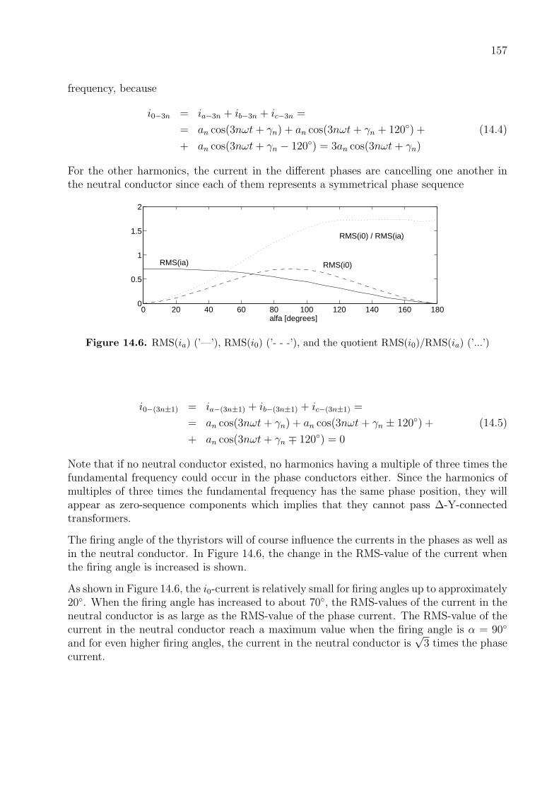
157
frequency, because
i0−3n = ia−3n + ib−3n + ic−3n =
= an cos(3nωt + γn) + an cos(3nωt + γn + 120) + (14.4)
+ an cos(3nωt + γn − 120) = 3an cos(3nωt + γn)
For the other harmonics, the current in the different phases are cancelling one another inthe neutral conductor since each of them represents a symmetrical phase sequence
0 20 40 60 80 100 120 140 160 1800
0.5
1
1.5
2
RMS(ia) RMS(i0)
RMS(i0) / RMS(ia)
alfa [degrees]
Figure 14.6. RMS(ia) (’—’), RMS(i0) (’- - -’), and the quotient RMS(i0)/RMS(ia) (’...’)
i0−(3n±1) = ia−(3n±1) + ib−(3n±1) + ic−(3n±1) =
= an cos(3nωt + γn) + an cos(3nωt + γn ± 120) + (14.5)
+ an cos(3nωt + γn ∓ 120) = 0
Note that if no neutral conductor existed, no harmonics having a multiple of three times thefundamental frequency could occur in the phase conductors either. Since the harmonics ofmultiples of three times the fundamental frequency has the same phase position, they willappear as zero-sequence components which implies that they cannot pass ∆-Y-connectedtransformers.
The firing angle of the thyristors will of course influence the currents in the phases as well asin the neutral conductor. In Figure 14.6, the change in the RMS-value of the current whenthe firing angle is increased is shown.
As shown in Figure 14.6, the i0-current is relatively small for firing angles up to approximately20. When the firing angle has increased to about 70, the RMS-values of the current in theneutral conductor is as large as the RMS-value of the phase current. The RMS-value of thecurrent in the neutral conductor reach a maximum value when the firing angle is α = 90
and for even higher firing angles, the current in the neutral conductor is√
3 times the phasecurrent.

158 14. Power system harmonics

Appendix A
MATLAB-codes for Examples 7.2, 7.3, 13.2and 13.3
%--- Example 7.2
l=5 ;
zled=0.9+j*0.3 ;
yled=j*3e-6 ;
%
pind=0.400 ;
cosind=0.8 ;
uind=10 ;
%
ik=-j*0.3 ;
uk=70 ;
%
stra=5 ;
xtraproc=4 ;
%--- Select base values
Sb=0.5 ;
Ub10=10 ;
Ub70=70 ;
Ib10=Sb/sqrt(3)/Ub10 ;
Ib70=Sb/sqrt(3)/Ub70 ;
Zb10=Ub10^2/Sb ;
%--- Calculate per-unit values for the Thevenin equivalent
Uthpu=uk/Ub70 ;
Zthpu=uk/Ub70*Ib70/ik ;
%--- Calculate per-unit values for the transformer
ztra=j*xtraproc/100*Sb/stra ;
%--- Calculate per-unit values for the line
LZ = zled*l/Zb10 ;
LY = yled*l*Zb10 ;
LA = 1+0.5*LY*LZ ;
LB = LZ ;
LC = LY*(1+0.25*LY*LZ) ;
LD = LA ;
%--- Calculate per-unit values for the industry impedance
Zindpu=uind^2/(pind/cosind)*(cosind+j*sqrt(1-cosind^2))/Zb10 ;
%--- Calculate the two port matrix for grid+transformer+line
fyrpol = [1 Zthpu ; 0 1]*[1 ztra ; 0 1]*[LA LB ; LC LD] ;
A= fyrpol(1,1) ;
B= fyrpol(1,2) ;
159

160 A. MATLAB-codes for Examples 7.2, 7.3, 13.2 and 13.3
C= fyrpol(2,1) ;
D= fyrpol(2,2) ;
%--- Calculate the total impedance of the grid
Ztot = (A*Zindpu+B)/(C*Zindpu+D) ;
i1 = Uthpu/Ztot ;
%--- Calculate u2 and i2
trakramat=[1 Zthpu+ztra ; 0 1] ;
u2i2=inv(trakramat)*[Uthpu ;i1] ;
s2=u2i2(1)*conj(u2i2(2))*Sb ;
%--- Calculate the voltage at the industry
matmat = [A B ; C D] ;
u3i3=inv(matmat)*[Uthpu ;i1] ;
u3=u3i3(1)*Ub10 ;
%--- Example 7.3
l1=2 ;
l2=1 ;
zled=0.17+j*0.3 ;
yled=j*3.2e-6 ;
%
pld1=0.500 ;
cosld1=0.8 ;
uld1=10 ;
pld2=0.200 ;
cosld2=0.95 ;
uld2=0.4 ;
%
st1=0.8 ;
xt1proc=7 ;
st2=0.3 ;
xt2proc=8 ;
%--- Select base values
Sb=0.5 ;
Ub10=10 ;
Ub04=0.4 ;
Ib10=Sb/sqrt(3)/Ub10 ;
Ib04=Sb/sqrt(3)/Ub04 ;
Zb10=Ub10^2/Sb ;
Zb04=Ub04^2/Sb ;
%--- Calculate per-unit values for the strong grid
u1=1 ;
%--- Calculate per-unit values for transformer T1
zT1pu=j*xt1proc/100*Sb/st1 ;
%--- Calculate per-unit values for transformen T2
zT2pu=j*xt2proc/100*Sb/st2 ;

161
%--- Calculate per-unit values for line L1
zL1pu = zled*l1/Zb10 ;
yL1pu = yled*l1*Zb10 ;
%--- Calculate per-unit values for line L2
zL2pu = zled*l2/Zb10 ;
yL2pu = yled*l2*Zb10 ;
%--- Calculate per-unit values for the LD1-impedance
zLD1pu=uld1^2/(pld1/cosld1)*(cosld1+j*sqrt(1-cosld1^2))/Zb10 ;
%--- Calculate per-unit values for the LD2-impedance
zLD2pu=uld2^2/(pld2/cosld2)*(cosld2+j*sqrt(1-cosld2^2))/Zb04 ;
%--- Formulate the Y-bus matrix for the grid
y22=1/zT1pu+1/zL1pu+(yL1pu/2)+1/zL2pu+(yL2pu/2) ;
y33=1/zL1pu+(yL1pu/2)+1/zLD1pu ;
y44=1/zL2pu+(yL2pu/2)+1/zT2pu ;
Ybus=[1/zT1pu -1/zT1pu 0 0 0 ; -1/zT1pu y22 -1/zL1pu -1/zL2pu 0 ;
0 -1/zL1pu y33 0 0 ; 0 -1/zL2pu 0 y44 -1/zT2pu ;
0 0 0 -1/zT2pu 1/zT2pu+1/zLD2pu] ;
Zbus=inv(Ybus) ;
%--- Calculate the efficiency
i1=u1/Zbus(1,1) ;
u2=Zbus(1,2)*i1 ;
u3=Zbus(1,3)*i1 ;
u4=Zbus(1,4)*i1 ;
u5=Zbus(1,5)*i1 ;
S1=u1*conj(i1)*Sb ;
iL1=(u2-u3)/zL1pu ;
PfL1=real(zL1pu)*abs(iL1)^2*Sb ;
iL2=(u2-u4)/zL2pu ;
PfL2=real(zL2pu)*abs(iL2)^2*Sb ;
verkn=100*( real(S1)-PfL1-PfL2 )/real(S1) ;
%---Calculation of the Z-bus matrix for fault current calculations
Ybusk=Ybus(2:5,2:5) ;
Zbusk=inv(Ybusk) ;
ik4 = u4/Zbusk(3,3)*Ib10 ;
%--- Example 13.2
alfa = exp(j*120*pi/180) ;
tmat = [1 1 1 ; alfa*alfa alfa 1 ; alfa alfa*alfa 1 ] ;
l=5 ;
zled1=0.9+j*0.3 ;
zledz=3*zled1 ;
yled1=j*3e-6 ;
yledz=0.5*yled1 ;
%
pind=0.400 ;

162 A. MATLAB-codes for Examples 7.2, 7.3, 13.2 and 13.3
cosind=0.8 ;
uind=10 ;
fasafaktor=2 ;
%
ik3=-j*0.3 ;
ik1=-j*0.2 ;
uk=70 ;
%
stra=5 ;
xtraproc=4 ;
%--- Select base values
Sb=0.5 ;
Ub10=10 ;
Ub70=70 ;
Ib10=Sb/sqrt(3)/Ub10 ;
Ib70=Sb/sqrt(3)/Ub70 ;
Zb10=Ub10^2/Sb ;
Zb70=Ub70^2/Sb ;
%--- Calculate per-unit values for the Thevenin equivalent
Uthpu=uk/Ub70 ;
Zthpu1=uk/Ub70*Ib70/ik3 ;
Zthpuz=3*uk/Ub70*Ib70/ik1-2*Zthpu1 ;
%--- Calculate per-unit values for the transformer
Ztrapu1=j*xtraproc/100*Sb/stra ;
Ztrapuz=Ztrapu1 ;
%--- Calculate per-unit values for the line
Zlpu1 = zled1*l/Zb10 ;
Zlpuz = zledz*l/Zb10 ;
Ylpu1 = yled1*l*Zb10 ;
Ylpuz = yledz*l*Zb10 ;
AL1 = 1+0.5*Ylpu1*Zlpu1 ;
BL1 = Zlpu1 ;
CL1 = Ylpu1*(1+0.25*Ylpu1*Zlpu1) ;
DL1 = AL1 ;
ALz = 1+0.5*Ylpuz*Zlpuz ;
BLz = Zlpuz ;
CLz = Ylpuz*(1+0.25*Ylpuz*Zlpuz) ;
DLz = ALz ;
%--- Calculate the positive sequence two-port matrix for grid+traf+line
plusmat = [1 Zthpu1 ; 0 1]*[1 Ztrapu1 ; 0 1]*[AL1 BL1 ; CL1 DL1] ;
A1= plusmat(1,1) ;
B1= plusmat(1,2) ;
C1= plusmat(2,1) ;
D1= plusmat(2,2) ;
UThc=Uthpu/A1 ;
ZThC1=B1/A1 ;

163
ZThC2=ZThC1 ;
%--- Calculate the two-port matrix for traf+line
nollmat = [1 Ztrapu1 ; 0 1]*[ALz BLz ; CLz DLz] ;
Az= nollmat(1,1) ;
Bz= nollmat(1,2) ;
Cz= nollmat(2,1) ;
Dz= nollmat(2,2) ;
ZThCz=Bz/Az ;
Zs=[ZThC1 0 0 ; 0 ZThC2 0 ; 0 0 ZThCz] ;
%--- Calculate the per-unit val. for ind. load imp. under normal conditions
Zindpu=uind^2/(pind/cosind)*(cosind+j*sqrt(1-cosind^2))/Zb10 ;
Zlds=inv(tmat)*[fasafaktor*Zindpu 0 0 ; 0 Zindpu 0 ; 0 0 Zindpu]*tmat ;
%--- Calculate symm. comp. for currents at the industry
Is=inv(Zs+Zlds)*[UThc ;0 ;0] ;
%--- Calculate symm. comp. for voltages at the industry
Uc=Zlds*Is ;
%--- Calculate the pos. seq. voltage and current from traf to line
UBIB1 = [AL1 BL1 ; CL1 DL1]*[Uc(1) ; Is(1)] ;
UB1 = UBIB1(1) ;
IB1 = UBIB1(2) ;
SB1=UB1*conj(IB1)*Sb ;
%--- Calculate the neg. seq. voltage and current from traf to line
UBIB2 = [AL1 BL1 ; CL1 DL1]*[Uc(2) ; Is(2)] ;
UB2 = UBIB2(1) ;
IB2 = UBIB2(2) ;
SB2=UB2*conj(IB2)*Sb ;
%--- Calculate the zero seq. voltage and current from traf to line
UBIBz = [ALz BLz ; CLz DLz]*[Uc(3) ; Is(3)] ;
UBz = UBIBz(1) ;
IBz = UBIBz(2) ;
SBz=UBz*conj(IBz)*Sb ;
%--- Calculate the phase components for the voltage at the industry
Ucf=tmat*Uc ;
%--- Calculate total delivered power from transformer to line
Stot=SB1+SB2+SBz ;
%--- Example 13.3
alfa = exp(j*120*pi/180) ;
tmat = [1 1 1 ; alfa*alfa alfa 1 ; alfa alfa*alfa 1 ] ;
%
l1=2 ;
l2=1 ;
zled=0.17+j*0.3 ;
yled=j*3.2e-6 ;
zledz=3*zled ;

164 A. MATLAB-codes for Examples 7.2, 7.3, 13.2 and 13.3
yledz=0.5*yled ;
%
pld1=0.500 ;
cosld1=0.8 ;
uld1=10 ;
pld2=0.200 ;
cosld2=0.95 ;
uld2=0.4 ;
%fasafaktor=2 ;
%
st1=0.8 ;
xt1proc=7 ;
st2=0.3 ;
xt2proc=8 ;
%
%--- Select base values
Sb=0.5 ;
Ub10=10 ;
Ub04=0.4 ;
Ib10=Sb/sqrt(3)/Ub10 ;
Ib04=Sb/sqrt(3)/Ub04 ;
Zb10=Ub10^2/Sb ;
Zb04=Ub04^2/Sb ;
%
%--- Calculate pur-unit-values for the strong grid
u1=1 ;
%
%--- Calculate pur-unit-values for transformer T1
zT1_1=j*xt1proc/100*Sb/st1 ;
zT1_z=zT1_1 ;
%
%--- Calculate pur-unit-values for transformer T2
zT2_1=j*xt2proc/100*Sb/st2 ;
zT2_z=zT2_1 ;
%
%--- Calculate pur-unit-values for line L1
zL1_1 = zled*l1/Zb10 ;
zL1_2 = zL1_1 ;
yL1_1 = yled*l1*Zb10 ;
zL1_z = zledz*l1/Zb10 ;
yL1_z = yledz*l1*Zb10 ;
%
%--- Calculate pur-unit-values for line L2
zL2_1 = zled*l2/Zb10 ;
zL2_2 = zL2_1 ;
yL2_1 = yled*l2*Zb10 ;
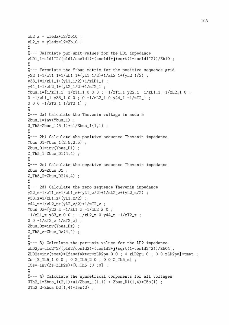
165
zL2_z = zledz*l2/Zb10 ;
yL2_z = yledz*l2*Zb10 ;
%
%--- Calculate pur-unit-values for the LD1 impedance
zLD1_1=uld1^2/(pld1/cosld1)*(cosld1+j*sqrt(1-cosld1^2))/Zb10 ;
%
%--- Formulate the Y-bus matrix for the positive sequence grid
y22_1=1/zT1_1+1/zL1_1+(yL1_1/2)+1/zL2_1+(yL2_1/2) ;
y33_1=1/zL1_1+(yL1_1/2)+1/zLD1_1 ;
y44_1=1/zL2_1+(yL2_1/2)+1/zT2_1 ;
Ybus_1=[1/zT1_1 -1/zT1_1 0 0 0 ; -1/zT1_1 y22_1 -1/zL1_1 -1/zL2_1 0 ;
0 -1/zL1_1 y33_1 0 0 ; 0 -1/zL2_1 0 y44_1 -1/zT2_1 ;
0 0 0 -1/zT2_1 1/zT2_1] ;
%
%--- 2a) Calculate the Thevenin voltage in node 5
Zbus_1=inv(Ybus_1) ;
U_Th5=Zbus_1(5,1)*u1/Zbus_1(1,1) ;
%
%--- 2b) Calculate the positive sequence Thevenin impedance
Ybus_D1=Ybus_1(2:5,2:5) ;
Zbus_D1=inv(Ybus_D1) ;
Z_Th5_1=Zbus_D1(4,4) ;
%
%--- 2c) Calculate the negative sequence Thevenin impedance
Zbus_D2=Zbus_D1 ;
Z_Th5_2=Zbus_D2(4,4) ;
%
%--- 2d) Calculate the zero sequence Thevenin impedance
y22_z=1/zT1_z+1/zL1_z+(yL1_z/2)+1/zL2_z+(yL2_z/2) ;
y33_z=1/zL1_z+(yL1_z/2) ;
y44_z=1/zL2_z+(yL2_z/2)+1/zT2_z ;
Ybus_Dz=[y22_z -1/zL1_z -1/zL2_z 0 ;
-1/zL1_z y33_z 0 0 ; -1/zL2_z 0 y44_z -1/zT2_z ;
0 0 -1/zT2_z 1/zT2_z] ;
Zbus_Dz=inv(Ybus_Dz) ;
Z_Th5_z=Zbus_Dz(4,4) ;
%
%--- 3) Calculate the per-unit values for the LD2 impedance
zLD2pu=uld2^2/(pld2/cosld2)*(cosld2+j*sqrt(1-cosld2^2))/Zb04 ;
ZLD2s=inv(tmat)*[fasafaktor*zLD2pu 0 0 ; 0 zLD2pu 0 ; 0 0 zLD2pu]*tmat ;
Zs=[Z_Th5_1 0 0 ; 0 Z_Th5_2 0 ; 0 0 Z_Th5_z] ;
I5s=-inv(Zs+ZLD2s)*[U_Th5 ;0 ;0] ;
%
%--- 4) Calculate the symmetrical components for all voltages
UTh2_1=Zbus_1(2,1)*u1/Zbus_1(1,1) + Zbus_D1(1,4)*I5s(1) ;
UTh2_2=Zbus_D2(1,4)*I5s(2) ;

166 A. MATLAB-codes for Examples 7.2, 7.3, 13.2 and 13.3
UTh2_z=Zbus_Dz(1,4)*I5s(3) ;
UTh3_1=Zbus_1(3,1)*u1/Zbus_1(1,1) + Zbus_D1(2,4)*I5s(1) ;
UTh3_2=Zbus_D2(2,4)*I5s(2) ;
UTh3_z=Zbus_Dz(2,4)*I5s(3) ;
UTh4_1=Zbus_1(4,1)*u1/Zbus_1(1,1) + Zbus_D1(3,4)*I5s(1) ;
UTh4_2=Zbus_D2(3,4)*I5s(2) ;
UTh4_z=Zbus_Dz(3,4)*I5s(3) ;
UTh5_1=Zbus_1(5,1)*u1/Zbus_1(1,1) + Zbus_D1(4,4)*I5s(1) ;
UTh5_2=Zbus_D2(4,4)*I5s(2) ;
UTh5_z=Zbus_Dz(4,4)*I5s(3) ;
%
%--- 5) Calculate pos., neg., and zero sequence currents through lines
IL1_1=(UTh2_1-UTh3_1)/zL1_1 ;
IL1_2=(UTh2_2-UTh3_2)/zL1_2 ;
IL1_z=(UTh2_z-UTh3_z)/zL1_z ;
IL2_1=(UTh2_1-UTh4_1)/zL2_1 ;
IL2_2=(UTh2_2-UTh4_2)/zL2_2 ;
IL2_z=(UTh2_z-UTh4_z)/zL2_z ;
ILD1_1=UTh3_1/zLD1_1 ;
ILD1_2=UTh3_2/zLD1_1 ;
ILD1_z=UTh3_z/zLD1_1 ;
%
%--- Calculation of efficiency
SL1_n2_1=UTh2_1*conj(IL1_1) ;
SL1_n2_2=UTh2_2*conj(IL1_2) ;
SL1_n2_z=UTh2_z*conj(IL1_z) ;
SL1_n2=Sb*(SL1_n2_1+SL1_n2_2+SL1_n2_z) ;
SL1_n3_1=UTh3_1*conj(IL1_1) ;
SL1_n3_2=UTh3_2*conj(IL1_2) ;
SL1_n3_z=UTh3_z*conj(IL1_z) ;
SL1_n3=Sb*(SL1_n3_1+SL1_n3_2+SL1_n3_z) ;
SL2_n2_1=UTh2_1*conj(IL2_1) ;
SL2_n2_2=UTh2_2*conj(IL2_2) ;
SL2_n2_z=UTh2_z*conj(IL2_z) ;
SL2_n2=Sb*(SL2_n2_1+SL2_n2_2+SL2_n2_z) ;
SL2_n4_1=UTh4_1*conj(IL2_1) ;
SL2_n4_2=UTh4_2*conj(IL2_2) ;
SL2_n4_z=UTh4_z*conj(IL2_z) ;
SL2_n4=Sb*(SL2_n4_1+SL2_n4_2+SL2_n4_z) ;
verkn=100*( real(SL1_n3)+real(SL2_n4 ))/(real(SL1_n2)+real(SL2_n2))

Appendix B
Matlab-codes for Example 8.10
% Start of file
clear,
clear global
deg=180/pi;
maxiter=10;
EPS=1e-4;
k1=-0.2; k2=1.2; k3=-0.07; k4=0.4;
% Step 1
converged=0; iter=0; x=3/deg;
while ~converged & iter < maxiter,
% Step 2
delta_gx=k4-(k1*x+k2*cos(x-k3));
% Step 3
if all(abs(delta_gx)< EPS),
converged=1;
iter=iter,
xdeg=x*deg
else
% Step 4
Jac=k1-k2*sin(x-k3); %Jac=dfx/dx;
% Step 5
delta_x=inv(Jac)*delta_gx;
% Step 6
x=x+delta_x;
iter=iter+1;
end, % if all
if iter==maxiter,
iter=iter,
disp(’The equation has no solutions’)
disp(’or’)
disp(’bad initial value, try with another initial value’)
end, % iter
end, % while
% End of file
167

168 B. Matlab-codes for Example 8.10

Appendix C
Matlab-codes for Example 8.12
% Start of file
clear,
clear global
deg=180/pi;
rad=1/deg;
nbus=3; %Number of buses
%Step 1
% 1a)
U1=1; theta1=0; PD1=0; QD1=0;
U2=1; PG2=2; PD2=1; QD2=0.2;
PG3=0; QG3=0; PD3=2; QD3=-0.4;
Z12=j*0.2; y12=1/Z12;
Z13=j*0.4; y13=1/Z13;
Z23=j*0.5; y23=1/Z23;
y11=y12+y13; y22=y12+y23; y33=y13+y23;
%1b)
Y=[y11 -y12 -y13 ; -y12 y22 -y23 ; -y13 -y23 y33];
G=real(Y);
B=imag(Y);
PGD2=PG2-PD2;
PGD3=PG3-PD3;
QGD3=QG3-QD3;
%1c)
%Bus 1 is slack bus
%Bus 2 is PU-bus
%Bus 3 is PQ-bus
bus1=1; bus2=2; bus3=3;
n_pu_pq=2; %number of PU-buses and PQ-buses
PGD=[PGD2;PGD3];
QGD=[QGD3];
%1d)
169

170 C. Matlab-codes for Example 8.12
theta2=0;
U3=1;
theta3=0;
iter=0;
VOLT=[U1;U2;U3];
ANG=[theta1;theta2;theta3];
while iter <4
% Step 2
%2a)
for m=1:nbus
for n=1:nbus
PP(m,n)=VOLT(m)*VOLT(n)*(G(m,n)*cos(ANG(m)-ANG(n))+B(m,n)*sin(ANG(m)-ANG(n)));
QQ(m,n)=VOLT(m)*VOLT(n)*(G(m,n)*sin(ANG(m)-ANG(n))-B(m,n)*cos(ANG(m)-ANG(n)));
end, %for n
end, % for m
P=sum(PP’); Q=sum(QQ’);
%2b)
deltaP=PGD-P([bus2 bus3])’;
deltaQ=QGD-Q([bus3])’;
% Step 4
%4a)
for m=1:nbus
for n=1:nbus
if m==n,
H(m,m)=-Q(m)-B(m,m)*VOLT(m)*VOLT(m);
N(m,m)= P(m)+G(m,m)*VOLT(m)*VOLT(m);
J(m,m)= P(m)-G(m,m)*VOLT(m)*VOLT(m);
L(m,m)= Q(m)-B(m,m)*VOLT(m)*VOLT(m);
else
H(m,n)= VOLT(m)*VOLT(n)*(G(m,n)*sin(ANG(m)-ANG(n))-B(m,n)*cos(ANG(m)-ANG(n)));
N(m,n)= VOLT(m)*VOLT(n)*(G(m,n)*cos(ANG(m)-ANG(n))+B(m,n)*sin(ANG(m)-ANG(n)));
J(m,n)=-VOLT(m)*VOLT(n)*(G(m,n)*cos(ANG(m)-ANG(n))+B(m,n)*sin(ANG(m)-ANG(n)));
L(m,n)= VOLT(m)*VOLT(n)*(G(m,n)*sin(ANG(m)-ANG(n))-B(m,n)*cos(ANG(m)-ANG(n)));
end, %if
end, %for n
end, % for m
H(bus1,:)=[]; H(:,bus1)=[]; N(bus1,:)=[]; N(:,[bus1 bus2])=[];
J([bus1 bus2],:)=[];J(:,bus1)=[]; L([bus1 bus2],:)=[]; L(:,[bus1 bus2])=[];
JAC=[H N ; J L];

171
% Step 5
%5a)
DX=inv(JAC)*[deltaP;deltaQ];
delta_theta=DX(1:n_pu_pq);
delta_U=DX(n_pu_pq+1:length(DX));
% Step 6
%6a)
iter=iter+1;
ANG([bus2 bus3])=ANG([bus2 bus3])+delta_theta;
VOLT([bus3])=VOLT([bus3]).*(1+delta_U);
end, %while
% Step 3
%3b)
for m=1:nbus
for n=1:nbus
PP(m,n)=VOLT(m)*VOLT(n)*(G(m,n)*cos(ANG(m)-ANG(n))+B(m,n)*sin(ANG(m)-ANG(n)));
QQ(m,n)=VOLT(m)*VOLT(n)*(G(m,n)*sin(ANG(m)-ANG(n))-B(m,n)*cos(ANG(m)-ANG(n)));
end, %for n
end, % for m
P=sum(PP’);
Q=sum(QQ’);
PG1=P(bus1)+PD1,
QG1=Q(bus1)+QD1,
QG2=Q(bus2)+QD2,
% End of file