UNIVERSITÀ DEGLI STUDI DI PADOVA, FACOLTÀ DI INGEGNERIACORSO DI LAUREA MAGISTRALE IN BIOINGEGNERIA

TESI DI LAUREA MAGISTRALE

Modellazione Numerica della Microscopia aForza Atomica (AFM) per la stima diparamentri da cellule fibroblastiche

Relatore Università di Padova: Prof. Alfredo RuggeriRelatore Royal Institute of Technology (KTH) : Prof. Christian GasserCorrelatore: M.Sc. Jacopo Biasetti

Laureando: Giulio Ferrazzi

Anno accademico : 2011/12

Acknowledgements

This master thesis was carried out at the Department of Solid Mechanics at the Royal Institudeof Technology (KTH), Sweden.

I want to express my sincere gratitude to my supervisor Prof. T. Christian Gasser for hisguidance and support in the course of this project.

Many special thanks to Jacopo Biasetti, M.Sc. , for his never - ending help in teaching me somany technical skills.

Finally, I would like to thank the sincere support of my family and my friends.

Stockholm, June 2011

Giulio Ferrazzi

Abstract

It has a long been known that many, if not all, diseases are associated with changes in the me-chanical properties of cells. Although these changes in tissue mechanics have been believed tobe a conseguense of the disease, recent data show that alterations of these mechanical propertieshave a potent effect to many cellular functions. Thus, there is no reason to believe that alteredcellular mechanics could be the cause of the disease, rather than its consequence. A completeunderstanding of cell mechanics and how the latter one depends on the presence of a disease istherefore necessary in order to develop methods of early diagnosis.

In this master thesis we report the preliminary results of fibroblast mechanics obtained bysimulating, in a numerical context, AFM (Atomic Force Microscopy).

Shortly, we tried to find out what is the relationship that coexists between the reaction force ofa fibroblast when subjected by this process of imaging. A subsequent process of reverse engineeringled to a simply analytical model for the quantification of the mechanical properties of cells. Thesecond part of this work aims to improve the understanding of the mechanotransduction mechanismof cells. Specifically, we report the results of soft contact and adhesion process of a fibroblast whenlaying on a polyacrylamide substrate. For last, we built up a numerical model that combines theassumptions of the first and the second part of this work.

Contents

I Introduction 1

1 AFM (Atomic Force Microscopy) 1

2 Cell - ECM contact 3

3 Objective of the thesis 3

II Linear elastic material behaviour 53.1 Other elastic constant: bulk, shear, and lamè modulus . . . . . . . . . . . . . . . . 5

III Hyperasticity material behaviour 6

4 Deformation measures used in finite elasticity 6

5 Calculating stress-strain relations from the strain energy density 7

6 A note on perfectly incopressible materials 7

7 Generalized neo-Hookean solid 7

IV AFM Model 8

8 2D Model (Central Indentation) 10

9 Validation 15

10 3D Model (Central Indentation) 17

11 3D Model (Lateral Indentation) 20

12 Evaluation of the shear modulus from the reaction force 23

V Simulation of the adhesive contact between fibroblasts and a poly-acrylamide substrate 25

VI Simulation of adhesive contact process with AFM indentation 32

VII Conclusion and future works 34

List of Figures1 Human fibroblast imaged by fluorescent microscopy . . . . . . . . . . . . . . . . . . 12 Shematic diagram showing the principles of AFM in contact mode . . . . . . . . . 23 Force versus relative deformation for a keratinocy cell . . . . . . . . . . . . . . . . 24 Cell-Substrate contact process . . . . . . . . . . . . . . . . . . . . . . . . . . . . . . 35 Geometry of AFM model (dimension in µm) . . . . . . . . . . . . . . . . . . . . . . 86 Geometry of AFM 2D model using axialsymmetry (dimension in µm) . . . . . . . 107 Mesh used in AFM 2D model (dimension in µm) . . . . . . . . . . . . . . . . . . . 118 Diplacement in z direction predicted by AFM 2D model for indentation values of

1.5, 2.5, 3.5 and 4.5 µm (dimension in µm) . . . . . . . . . . . . . . . . . . . . . . . 119 Diplacement in r direction predicted by AFM 2D model for indentation values of

1.5, 2.5, 3.5 and 4.5 µm (dimension in µm) . . . . . . . . . . . . . . . . . . . . . . . 1210 Undeformed and deformed geometry . . . . . . . . . . . . . . . . . . . . . . . . . . 1211 Deformed Mesh of AFM 2D model (dimension in µm) . . . . . . . . . . . . . . . . 1312 Normal stress in z direction predicted by AFM 2D model for indentation values of

1.5, 2.5, 3.5 and 4.5 µm (dimension in Pa). . . . . . . . . . . . . . . . . . . . . . . 1313 Reaction force versus average deformation predicted by the AFM 2D model . . . . 1414 Keranocytes measuraments set up . . . . . . . . . . . . . . . . . . . . . . . . . . . 1515 Diplacement in z direction predicted by AFM 2D model for keranocyte cell (dimen-

sion in µm) . . . . . . . . . . . . . . . . . . . . . . . . . . . . . . . . . . . . . . . . 1516 Reaction force predicted by 2D AFM model and measured reaction force versus

average deformation . . . . . . . . . . . . . . . . . . . . . . . . . . . . . . . . . . . 1617 Symmetry boundaries of AFM 3D model (dimension in µm) . . . . . . . . . . . . . 1718 Mesh used in AFM 3D model . . . . . . . . . . . . . . . . . . . . . . . . . . . . . . 1819 Diplacement in z direction predicted by AFM 3D model for indentation values of 4

µm (dimension in µm) . . . . . . . . . . . . . . . . . . . . . . . . . . . . . . . . . . 1820 Reaction force versus average deformation predicted by the AFM 3D model . . . . 1921 Geometry of AFM 3D model, lateral indentation of 16 and 31 µm (dimension in µm) 2022 Mesh used in AFM 3D model, lateral indentation of 31 µm . . . . . . . . . . . . . 2123 Diplacement in z direction predicted by AFM 3D model for indentation values of 1

µm, lateral indentation of 31 µm (dimension in µm) . . . . . . . . . . . . . . . . . 2224 Reaction force versus average deformation predicted by the AFM 3D model, central

indentation and lateral indentation of 16 and 31 µm . . . . . . . . . . . . . . . . . 2225 Comparison between normal stress (left) and shear stress (right) of 2D AFM model

(dimension in Pa). . . . . . . . . . . . . . . . . . . . . . . . . . . . . . . . . . . . . 2326 Shear modulus estimation for 1, 1.67, 2, 3 kPa . . . . . . . . . . . . . . . . . . . . 2427 Geometry of adhesion contact model (dimension in µm) . . . . . . . . . . . . . . . 2528 f(z) for adhesion contact model . . . . . . . . . . . . . . . . . . . . . . . . . . . . . 2629 Normal Vector to boudary 6 . . . . . . . . . . . . . . . . . . . . . . . . . . . . . . . 2630 Mesh for adhesion contact model (dimension in µm) . . . . . . . . . . . . . . . . . 2731 Diplacement in z direction for adhesion contact model for β values of 1060, 2060,

3060 and 4060, rigid substrate without nucleus (dimension in µm) . . . . . . . . . 2832 Geometry for adhesion contact model with nucleus (dimension in µm) . . . . . . . 2933 Diplacement in z direction for adhesion contact model for β values of 1060, 2060,

3060 and 4060, rigid substrate with nucleus (dimension in µm) . . . . . . . . . . . 2934 Diplacement in z direction for adhesion contact model for β values of 1060, 2060,

3060 and 4060, deformable substrate without nucleus (dimension in µm) . . . . . . 3035 Diplacement in z direction for adhesion contact model for β values of 1060, 2060,

3060 and 4060, deformable substrate with nucleus (dimension in µm) . . . . . . . . 3136 3D geometry of adhesive contact process with AFM considering the nucleus (dimen-

sion in µm) . . . . . . . . . . . . . . . . . . . . . . . . . . . . . . . . . . . . . . . . 3237 Diplacement in z direction predicted by AFM 2D model for an indentation values

of 2 µm respectively without and with nucleus (dimension in µm) . . . . . . . . . . 3338 Reaction forces versus indentation predicted by the AFM 2D model without and

with nucleus . . . . . . . . . . . . . . . . . . . . . . . . . . . . . . . . . . . . . . . . 33

Part I

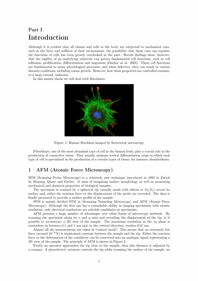
IntroductionAlthough it is evident that all tissues and cells in the body are subjected to mechanical cues,such as the force and stiffness of their environment, the possibility that these cues can regulatethe functions of cells has been greatly overlooked in the past. Recent findings show, however,that the rigidity of an underlying substrate can govern fundamental cell functions, such as celladhesion, proliferation, differentiation and migration (Discher at al. 2005). These cell functionsare fundamental to many physiological processes, and when defective, they can result in variousdiseases conditions, including tumor growth. However, how these properties are controlled remains,to a large extend, unknown.

In this master thesis we will deal with fibroblasts.

Figure 1: Human fibroblast imaged by fluorescent microscopy

Fibroblasts, one of the most abundant type of cell in the human body, play a crucial role in theproduction of connective tissue. They usually undergo several differentiation steps in which eachtype of cell is specialized in the production of a certain types of tissue; for instance chondroblasts.

1 AFM (Atomic Force Microscopy)SPM (Scanning Probe Microscopy) is a relatively new technique introduced in 1992 in Zurichby Binning, Quate and Gerber. It aims of imagining surface morphology as well as measuringmechanical and chemical properties of biological samples.

The speciment is scanned by a spherical tip (usually made with silicon or Si3N4) across itssurface and, either the reaction force or the displacement of the probe are recorded. The data isfinally processed to provide a surface profile of the sample.

SPM is mainly divided STM in (Scanning Tunneling Microscopy) and AFM (Atomic ForceMicroscopy). Although the first one has a remarkable ability in imaging speciments with atomicresolution, only electrical conductors are suitable candidates as speciments.

AFM presents a large number of advantages over other forms of microscopy methods. Byscanning the speciment along its x and y axes and recording the displacement of the tip, is itpossible to reconstruct a 3D view of the sample. The maximum resolution in the xy plane issomewhere in between 0.1 and 1 nm and, in the vertical direction, reaches 0.01 nm.

Almost all the measurements are taken in “contact mode”. This means that an extremely lowforce (around 10−9N) is maintained constant between the sample and the tip. Either the reactionforce or the deformation of the cantiliever can be converted into an analogue signal representing a3D view of the sample. The principle of AFM is shown in Figure 2.

Firstly an operator approaches the tip close to the sample, then this distance is adjusted bya scanner. A piezoelectric actuator controls the tip while scanning the surface of the sample, no

1

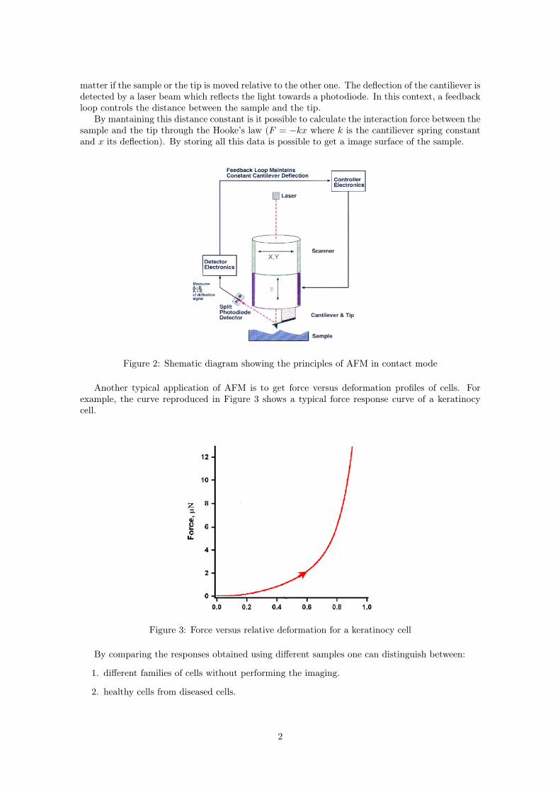
matter if the sample or the tip is moved relative to the other one. The deflection of the cantiliever isdetected by a laser beam which reflects the light towards a photodiode. In this context, a feedbackloop controls the distance between the sample and the tip.

By mantaining this distance constant is it possible to calculate the interaction force between thesample and the tip through the Hooke’s law (F = −kx where k is the cantiliever spring constantand x its deflection). By storing all this data is possible to get a image surface of the sample.

Figure 2: Shematic diagram showing the principles of AFM in contact mode

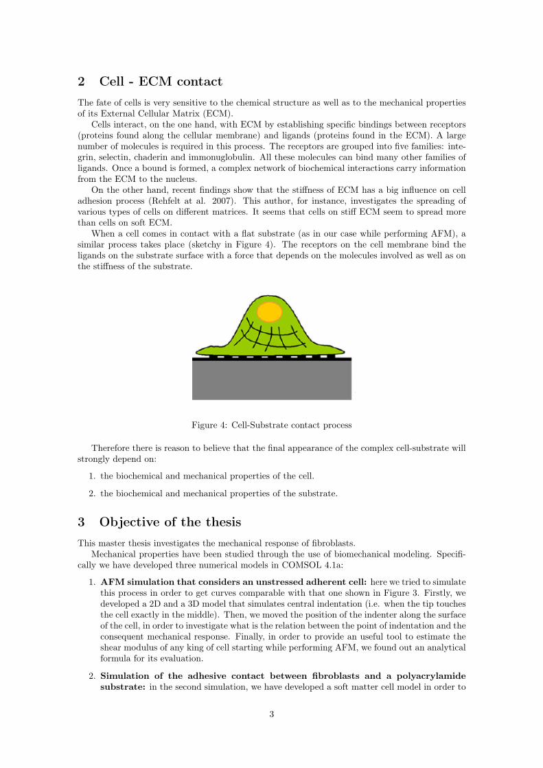
Another typical application of AFM is to get force versus deformation profiles of cells. Forexample, the curve reproduced in Figure 3 shows a typical force response curve of a keratinocycell.

Figure 3: Force versus relative deformation for a keratinocy cell

By comparing the responses obtained using different samples one can distinguish between:

1. different families of cells without performing the imaging.

2. healthy cells from diseased cells.

2

2 Cell - ECM contactThe fate of cells is very sensitive to the chemical structure as well as to the mechanical propertiesof its External Cellular Matrix (ECM).

Cells interact, on the one hand, with ECM by establishing specific bindings between receptors(proteins found along the cellular membrane) and ligands (proteins found in the ECM). A largenumber of molecules is required in this process. The receptors are grouped into five families: inte-grin, selectin, chaderin and immonuglobulin. All these molecules can bind many other families ofligands. Once a bound is formed, a complex network of biochemical interactions carry informationfrom the ECM to the nucleus.

On the other hand, recent findings show that the stiffness of ECM has a big influence on celladhesion process (Rehfelt at al. 2007). This author, for instance, investigates the spreading ofvarious types of cells on different matrices. It seems that cells on stiff ECM seem to spread morethan cells on soft ECM.

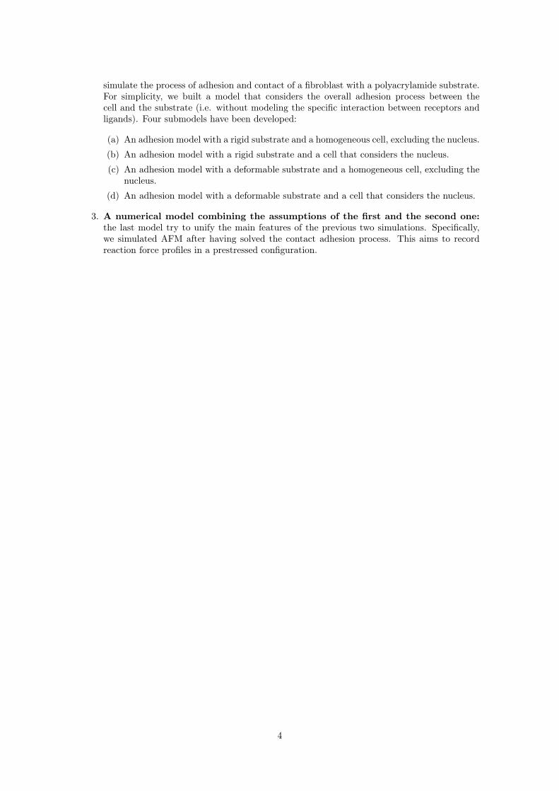
When a cell comes in contact with a flat substrate (as in our case while performing AFM), asimilar process takes place (sketchy in Figure 4). The receptors on the cell membrane bind theligands on the substrate surface with a force that depends on the molecules involved as well as onthe stiffness of the substrate.

Figure 4: Cell-Substrate contact process

Therefore there is reason to believe that the final appearance of the complex cell-substrate willstrongly depend on:

1. the biochemical and mechanical properties of the cell.

2. the biochemical and mechanical properties of the substrate.

3 Objective of the thesisThis master thesis investigates the mechanical response of fibroblasts.

Mechanical properties have been studied through the use of biomechanical modeling. Specifi-cally we have developed three numerical models in COMSOL 4.1a:

1. AFM simulation that considers an unstressed adherent cell: here we tried to simulatethis process in order to get curves comparable with that one shown in Figure 3. Firstly, wedeveloped a 2D and a 3D model that simulates central indentation (i.e. when the tip touchesthe cell exactly in the middle). Then, we moved the position of the indenter along the surfaceof the cell, in order to investigate what is the relation between the point of indentation and theconsequent mechanical response. Finally, in order to provide an useful tool to estimate theshear modulus of any king of cell starting while performing AFM, we found out an analyticalformula for its evaluation.

2. Simulation of the adhesive contact between fibroblasts and a polyacrylamidesubstrate: in the second simulation, we have developed a soft matter cell model in order to

3

simulate the process of adhesion and contact of a fibroblast with a polyacrylamide substrate.For simplicity, we built a model that considers the overall adhesion process between thecell and the substrate (i.e. without modeling the specific interaction between receptors andligands). Four submodels have been developed:

(a) An adhesion model with a rigid substrate and a homogeneous cell, excluding the nucleus.

(b) An adhesion model with a rigid substrate and a cell that considers the nucleus.

(c) An adhesion model with a deformable substrate and a homogeneous cell, excluding thenucleus.

(d) An adhesion model with a deformable substrate and a cell that considers the nucleus.

3. A numerical model combining the assumptions of the first and the second one:the last model try to unify the main features of the previous two simulations. Specifically,we simulated AFM after having solved the contact adhesion process. This aims to recordreaction force profiles in a prestressed configuration.

4

Part II

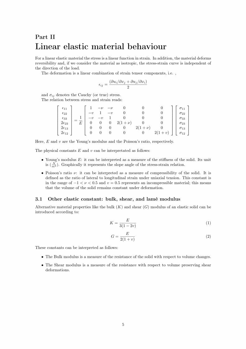
Linear elastic material behaviourFor a linear elastic material the stress is a linear function in strain. In addition, the material deformsreversibility and, if we consider the material as isotropic, the stress-strain curve is independent ofthe direction of the load.

The deformation is a linear combination of strain tensor components, i.e. ,

εij =(∂ui/∂xj + ∂uj/∂xi)

2

and σij denotes the Cauchy (or true) stress.The relation between stress and strain reads:

ε11ε22ε332ε232ε132ε12

=1

E

1 −ν −ν 0 0 0−v 1 −v 0 0 0−v −v 1 0 0 00 0 0 2(1 + ν) 0 00 0 0 0 2(1 + ν) 00 0 0 0 0 2(1 + v)

σ11σ22σ33σ23σ13σ12

Here, E and v are the Young’s modulus and the Poisson’s ratio, respectively.

The physical constants E and v can be interpretated as follows:

• Young’s modulus E: it can be interpreted as a measure of the stiffness of the solid. Its unitis ( N

m2 ). Graphically it represents the slope angle of the stress-strain relation.

• Poisson’s ratio ν: it can be interpreted as a measure of compressibility of the solid. It isdefined as the ratio of lateral to longitudinal strain under uniaxial tension. This constant isin the range of −1 < ν < 0.5 and v = 0.5 represents an incompressible material; this meansthat the volume of the solid remains constant under deformation.

3.1 Other elastic constant: bulk, shear, and lamè modulusAlternative material properties like the bulk (K) and shear (G) modulus of an elastic solid can beintroduced according to:

K =E

3(1− 2v)(1)

G =E

2(1 + v)(2)

These constants can be interpreted as follows:

• The Bulk modulus is a measure of the resistance of the solid with respect to volume changes.

• The Shear modulus is a measure of the resistance with respect to volume preserving sheardeformations.

5

Part III

Hyperasticity material behaviourElastic materials subjected to very large strains can mathematically be considered by hyperelasticconstitutive laws. With these models, we can describe the behavior of materials like rubbers,polimers and soft biological tissue.

An hyperelastic model is always constructed as follows:

1. A strain energy density W has to be defined as function of the deformation gradient tensorF. Thus, W = W (F).

2. For an isotropic material the strain energy density is a function of the left Cauchy-Greendeformation tensor B = F • FT. Then, to ensure that the constitutive equation is objective,the strain energy function must be a function of the invariants of B.

3. Stress-strain relations are obtained by differentiating W with respect to the strain.

4 Deformation measures used in finite elasticityIndicating with ui(xk) the displacement field of a solid, we define the following:

• Deformation gradient and its Jacobian:

Fij = δij +∂ui∂xj

, J = det(F)

• Left Cauchy-Green deformation tensor:

B = F • FT, Bij = FikFjk

• Invariants of B:I1 = tr(B) = Bkk

I2 =1

2(I21 −B : B) =

1

2(I21 −BikBki)

I3 = detB =J2

• To model incompressible materials, an alternative sets of invariants of B can be used:

I1 =I1

J23

=Bkk

J23

I2 =I2

J43

=1

2(I1

2 − B : B

J43

) =1

2(I1 −

BikBki

J43

)

J =√detB

6

5 Calculating stress-strain relations from the strain energydensity

In order to build the constitutive law one has to define an equation that relates the strain energydensity with the deformation gradient or with one of the set of the three invariants defined in theprevious section:

W (F) = U(I1, I2, I3) = U(I1, I2, J)

Formulas for the stress-strain relations are presented below. For simplicity we skip all thederivations:

• W in terms of Fij :

σij =1

JFik

∂W

∂Fjk

• W in terms of I1, I2, I3:

σij =2√I3

[(∂U

∂I1+ I1

∂U

∂I2)Bij −

∂U

∂I2BikBkj

]+ 2√I3∂U

∂I3δij

• W in tems of I1, I2, J :

σij =2

J

[1

J2/3(∂U

∂I1+ I1

∂U

∂I2)Bij − (I1

∂U

∂I1+ 2I2

∂U

∂I2)δij3− 1

J4/3

∂U

∂I2BikBkj

]+∂U

∂Jδij

6 A note on perfectly incopressible materialsMost of biological materials retains their volume during deformation. Therefore they can bemodeled as incompressible (or nearly incompressible) materials. Consequently:

• J is equal to one, therefore the strain energy density is solely a function of the first twoinvariants. Thus, U = U(I1, I2).

• The stress relation in terms of U(I1, I2) reads,

σij =

[2(∂U

∂I1+ I1

∂U

∂I2)Bij − (I1

∂U

∂I1+ 2I2

∂U

∂I2)δij3− ∂U

∂I2BikBkj

]+ pδij ,

where p is the hydrostatic stress. It’s an unknown variable witch has to be calculated bysolving a boundary problem.

7 Generalized neo-Hookean solidA neo-Hookean material is defined by:

U =µ1

2(I1 − 3) +

K1

2(J − 1)2, (3)

where µ1and K1are material properties (for small deformations, µ1and K1are the shear modulusand bulk modulus of the solid). This model should be used with K1 � µ1. The stress-strainrelation reads,

σij =µ1

J53

(Bij −1

3Bkkδij) +K1(J − 1)δij . (4)

The fully incompressible limit can be obtained by setting K1(J − 1) = p/3 in the shear stress law.

7

Part IV

AFM ModelHereafter we present the results of our simulations.

Useful information about the system have been gently provided by the Department of Micro-biology, Tumor and Cell Biology (MTC) of Karolinska Institute (KI), while the missing data wereestimated from the literature.

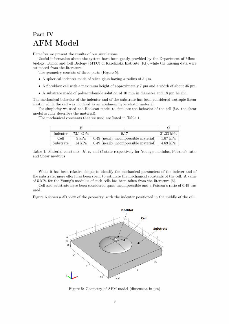
The geometry consists of three parts (Figure 5):

• A spherical indenter made of silica glass having a radius of 5 µm.

• A fibroblast cell with a maximum height of approximately 7 µm and a width of about 35 µm.

• A substrate made of polyacrylamide solution of 10 mm in diameter and 18 µm height.

The mechanical behavior of the indenter and of the substrate has been considered isotropic linearelastic, while the cell was modeled as an nonlinear hyperelastic material.

For simplicity we used neo-Hookean model to simulate the behavior of the cell (i.e. the shearmodulus fully describes the material).

The mechanical constants that we used are listed in Table 1.

E v G

Indenter 73.1 GPa 0.17 31.23 kPaCell 5 kPa 0.49 (nearly incompressible material) 1.67 kPa

Substrate 14 kPa 0.49 (nearly incompressible material) 4.69 kPa

Table 1: Material constants: E, υ, and G state respectively for Young’s modulus, Poisson’s ratioand Shear modulus

While it has been relative simple to identify the mechanical parameters of the indeter and ofthe substrate, more effort has been spent to estimate the mechanical constants of the cell. A valueof 5 kPa for the Young’s modulus of such cells has been taken from the literature [6].

Cell and substrate have been considered quasi incompressible and a Poisson’s ratio of 0.49 wasused.

Figure 5 shows a 3D view of the geometry, with the indenter positioned in the middle of the cell.

Figure 5: Geometry of AFM model (dimension in µm)

8

We modeled, in first approximation, the cell as an half ellipsoid of height 7 and width 35 µm.

The quasi-static solution was computed. Specifically, after having imposed a parametricdisplacement for the indenter, we recorded the reaction force. Finally force-deformation profileswere plotted.

9

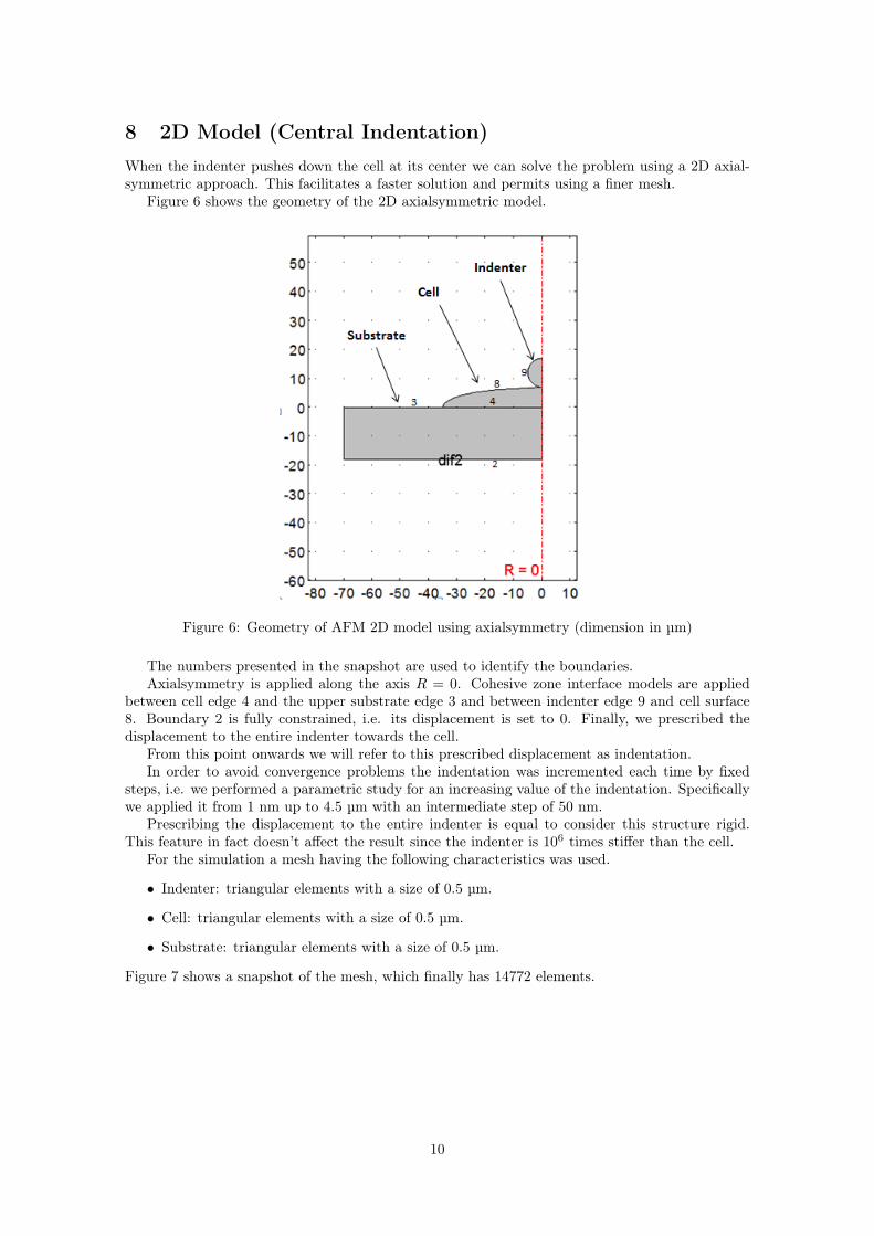
8 2D Model (Central Indentation)When the indenter pushes down the cell at its center we can solve the problem using a 2D axial-symmetric approach. This facilitates a faster solution and permits using a finer mesh.

Figure 6 shows the geometry of the 2D axialsymmetric model.

Figure 6: Geometry of AFM 2D model using axialsymmetry (dimension in µm)

The numbers presented in the snapshot are used to identify the boundaries.Axialsymmetry is applied along the axis R = 0. Cohesive zone interface models are applied

between cell edge 4 and the upper substrate edge 3 and between indenter edge 9 and cell surface8. Boundary 2 is fully constrained, i.e. its displacement is set to 0. Finally, we prescribed thedisplacement to the entire indenter towards the cell.

From this point onwards we will refer to this prescribed displacement as indentation.In order to avoid convergence problems the indentation was incremented each time by fixed

steps, i.e. we performed a parametric study for an increasing value of the indentation. Specificallywe applied it from 1 nm up to 4.5 µm with an intermediate step of 50 nm.

Prescribing the displacement to the entire indenter is equal to consider this structure rigid.This feature in fact doesn’t affect the result since the indenter is 106 times stiffer than the cell.

For the simulation a mesh having the following characteristics was used.

• Indenter: triangular elements with a size of 0.5 µm.

• Cell: triangular elements with a size of 0.5 µm.

• Substrate: triangular elements with a size of 0.5 µm.

Figure 7 shows a snapshot of the mesh, which finally has 14772 elements.

10

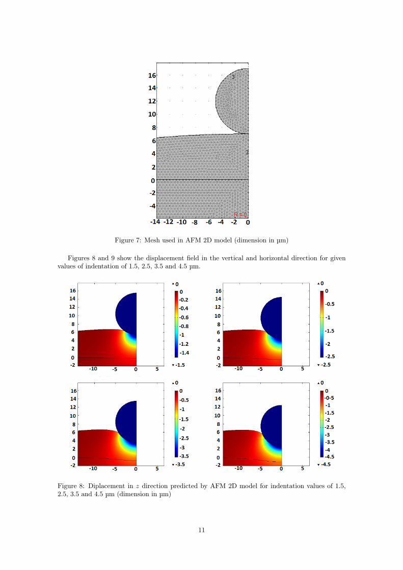
Figure 7: Mesh used in AFM 2D model (dimension in µm)

Figures 8 and 9 show the displacement field in the vertical and horizontal direction for givenvalues of indentation of 1.5, 2.5, 3.5 and 4.5 µm.

Figure 8: Diplacement in z direction predicted by AFM 2D model for indentation values of 1.5,2.5, 3.5 and 4.5 µm (dimension in µm)

11

Figure 9: Diplacement in r direction predicted by AFM 2D model for indentation values of 1.5,2.5, 3.5 and 4.5 µm (dimension in µm)

The 2D axialsymmetric model converged up to an average deformation of 0.65. Here, theaverage deformation is defined as ε = 1− 4h

h (Figure 10).

.

Figure 10: Undeformed and deformed geometry

Exceeding this deformation limit, the mesh deforms too much. A snapshot of the deformedmesh quality (close to the indentation site) is shown in Figure 11.

12

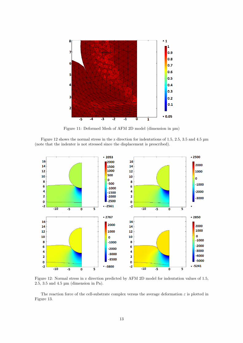
Figure 11: Deformed Mesh of AFM 2D model (dimension in µm)

Figure 12 shows the normal stress in the z direction for indentations of 1.5, 2.5, 3.5 and 4.5 µm(note that the indenter is not stressed since the displacement is prescribed).

Figure 12: Normal stress in z direction predicted by AFM 2D model for indentation values of 1.5,2.5, 3.5 and 4.5 µm (dimension in Pa).

The reaction force of the cell-substrate complex versus the average deformation ε is plotted inFigure 13.

13

Figure 13: Reaction force versus average deformation predicted by the AFM 2D model

The model predicts forces of the order of µN .

14

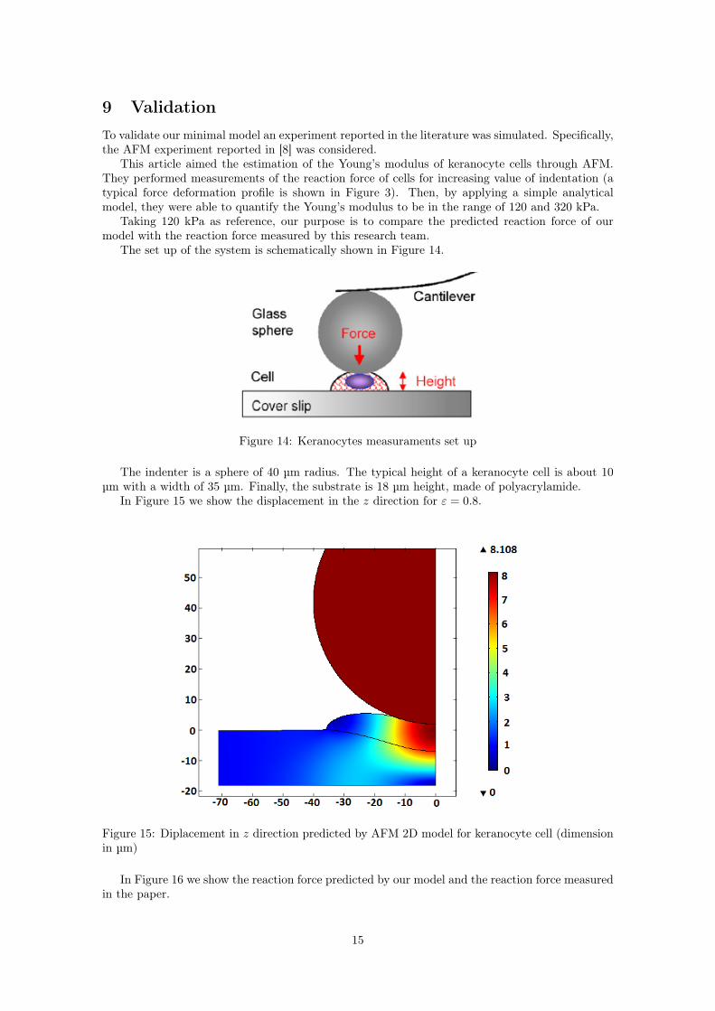
9 ValidationTo validate our minimal model an experiment reported in the literature was simulated. Specifically,the AFM experiment reported in [8] was considered.

This article aimed the estimation of the Young’s modulus of keranocyte cells through AFM.They performed measurements of the reaction force of cells for increasing value of indentation (atypical force deformation profile is shown in Figure 3). Then, by applying a simple analyticalmodel, they were able to quantify the Young’s modulus to be in the range of 120 and 320 kPa.

Taking 120 kPa as reference, our purpose is to compare the predicted reaction force of ourmodel with the reaction force measured by this research team.

The set up of the system is schematically shown in Figure 14.

Figure 14: Keranocytes measuraments set up

The indenter is a sphere of 40 µm radius. The typical height of a keranocyte cell is about 10µm with a width of 35 µm. Finally, the substrate is 18 µm height, made of polyacrylamide.

In Figure 15 we show the displacement in the z direction for ε = 0.8.

Figure 15: Diplacement in z direction predicted by AFM 2D model for keranocyte cell (dimensionin µm)

In Figure 16 we show the reaction force predicted by our model and the reaction force measuredin the paper.

15

Figure 16: Reaction force predicted by 2D AFM model and measured reaction force versus averagedeformation

Our model is able to quantify the reaction force of the cell in terms of order of magnitude.Anyway, the material seems to have an higher non linearity that cannot be described by neo-Hookean equation.

16

10 3D Model (Central Indentation)To validate the result obtained with the 2D axialsymmetric approach, we implemented a 3D modelfor central indentation. We can now exploit two planes of symmetry as shown in Figure 17.

Figure 17: Symmetry boundaries of AFM 3D model (dimension in µm)

The boundary conditions are the same of those ones introduced in the 2D model.Regarding the mesh, we tried to use the same element size of the 2D model but we ended up

with numerical problems (in this case indeed the number of elements was bigger the 200 000).As outlined from the solution of the 2D model, the cell presents a big stress gradient close to

the indentation site; far away from this area the stress is almost zero. We therefore defined a cubein which the mesh is extremely fine. Outside of this area the element size is bigger.

A snapshot of the mesh is shown in Figure 18.

17

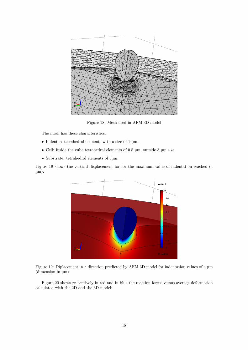
Figure 18: Mesh used in AFM 3D model

The mesh has these characteristics:

• Indenter: tetrahedral elements with a size of 1 µm.

• Cell: inside the cube tetrahedral elements of 0.5 µm, outside 3 µm size.

• Substrate: tetrahedral elements of 3µm.

Figure 19 shows the vertical displacement for for the maximum value of indentation reached (4µm).

Figure 19: Diplacement in z direction predicted by AFM 3D model for indentation values of 4 µm(dimension in µm)

Figure 20 shows respectively in red and in blue the reaction forces versus average deformationcalculated with the 2D and the 3D model:

18

Figure 20: Reaction force versus average deformation predicted by the AFM 3D model

The reaction forces are almost the same.

19

11 3D Model (Lateral Indentation)The indentation site is generally unknown; the indenter can touch the cell up to the nucleus aswell as in the periphery. Accordingly, the response of the material will be different with respect tothe position of indentation.

In the following simulation we changed the position of the indenter along the surface of the cell;specifically it has been moved through the x axis for values of 16 µm and 31 µm. The geometry isshown in Figure 21 (notice that we can exploit one symmetry in this case).

Figure 21: Geometry of AFM 3D model, lateral indentation of 16 and 31 µm (dimension in µm)

The mesh is shown in Figure 22.

20

Figure 22: Mesh used in AFM 3D model, lateral indentation of 31 µm

We need a fine mesh close to the indentation site, while the mesh can be coarse far away fromit. We used these elements:

• Indenter: tetrahedral elements with a size of 1 µm.

• Cell: tetrahedral elements with a minimum and maximum size of 0.1 µm and 5 µm, with agrowth rate of 1.1.

• Substrate: tetrahedral elements with a minimum and maximum size of 0.1 µm and 20 µmrespectively with a growth rate of 1.5.

Figure 23 shows the vertical displacement for a value of indentation of 1 µm.

21

Figure 23: Diplacement in z direction predicted by AFM 3D model for indentation values of 1 µm,lateral indentation of 31 µm (dimension in µm)

The reaction forces for different positions of the indentation of 0, 16 and 31 µm are shown inFigure 24 respectively in blue, green and red.

Figure 24: Reaction force versus average deformation predicted by the AFM 3D model, centralindentation and lateral indentation of 16 and 31 µm

From these graphs one can see that the mechanical response of a cell depends on the position ofindentation. The reaction force indeed is stiffer in the periphery (higher reaction force) rather thanin the center. This is due to the fact that, in the periphery, the system senses more the presenceof the substrate.

22

12 Evaluation of the shear modulus from the reaction forceOne of the main reason in performing AFM is to characterize mechanically the speciment. Here wepropose a rough estimation of the shear modulus starting from the knowledge of the indentationparameter and the reaction force (these are indeed the accessible variables to which the operatorhas easy access). We simulated the models presented so far for different values of an imposed shearmodulus and, after having recorded the reaction force, we estimated the latter parameter by usinga simple analytical formula.

The relationship between the shear modulus and the stress for a neo-Hookean incompressiblematerial is:

G =σ

λ+ λ−0.5

where λ = 1 + ε. ε represents the strain and σ the stress.The problem of estimating the shear modulus is, in this case, reduced in choosing a way to

estimate σ and ε.We chose, as a measure of ε, the average deformation introduced so far (this parameter varies

linearly with the indentation value).Regarding the estimation of σ, we made this considerations: if one compares the shear stress

with normal stress in the vertical direction, will realize that the latter is dominant. These twoquantities are reproduced in Figure 25.

Figure 25: Comparison between normal stress (left) and shear stress (right) of 2D AFM model(dimension in Pa).

Since the normal stress is dominant, we decided to neglect the shear component and to focusonly on the normal stress.

The latter has been estimated by using this formula:

σz =F

vπR2

where F is the reaction force, πR2 is equal to the area of the central section of the indenter,and v is a parameter that depends somehow on the indentation value. In order to fit the estimatedshear modulus with the actual shear modulus we chose:

v = a√INDENTATION

where a is a constant.We performed four simulations changing the value of the imposed shear modulus for 1, 1.67, 2,

3 kPa. The estimated value of the shear modulus versus indentation is reported in Figure 26.

23

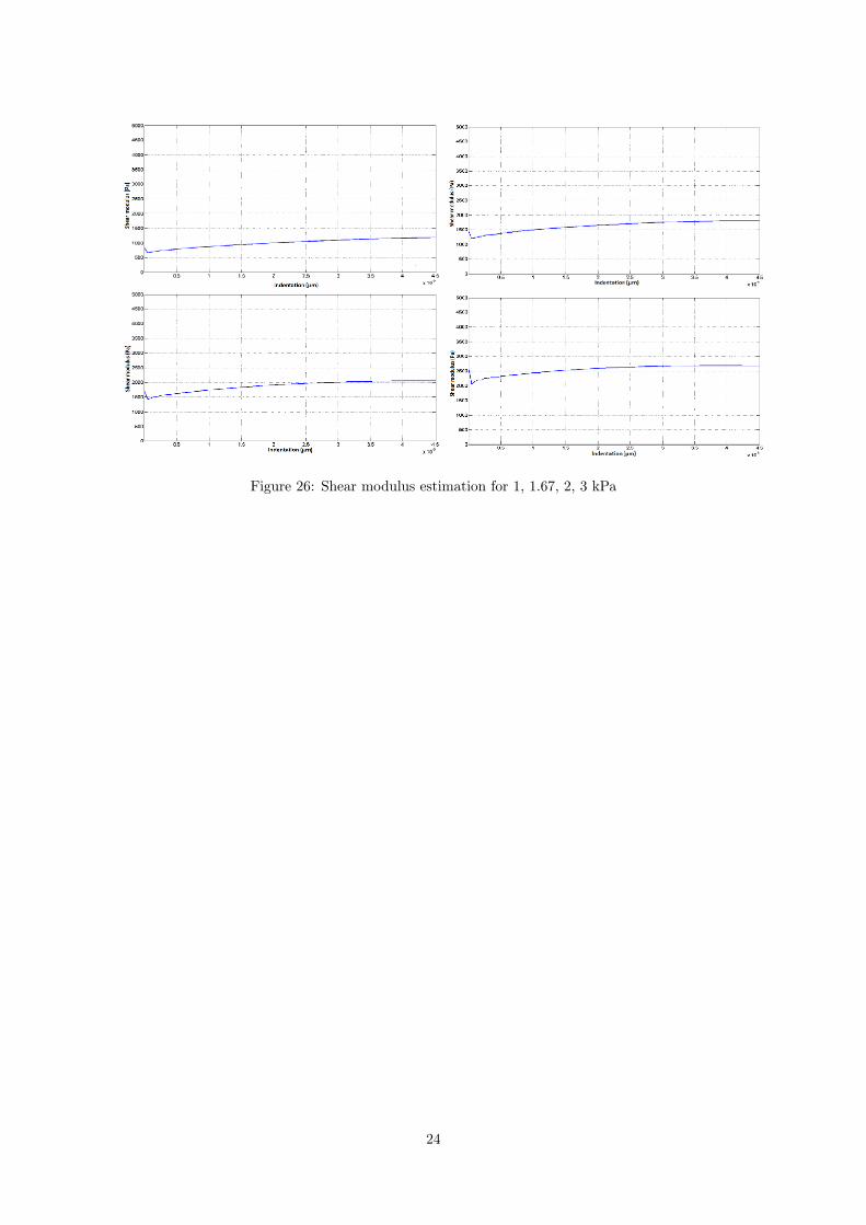
Figure 26: Shear modulus estimation for 1, 1.67, 2, 3 kPa

24

Part V

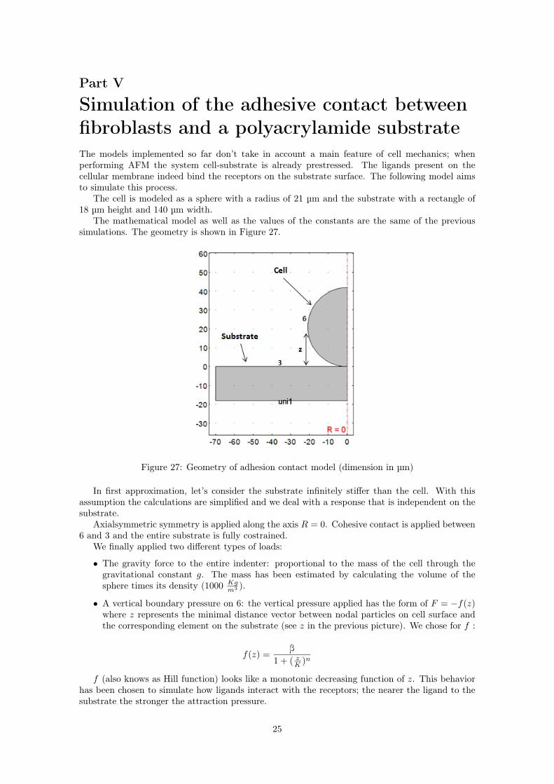
Simulation of the adhesive contact betweenfibroblasts and a polyacrylamide substrateThe models implemented so far don’t take in account a main feature of cell mechanics; whenperforming AFM the system cell-substrate is already prestressed. The ligands present on thecellular membrane indeed bind the receptors on the substrate surface. The following model aimsto simulate this process.

The cell is modeled as a sphere with a radius of 21 µm and the substrate with a rectangle of18 µm height and 140 µm width.

The mathematical model as well as the values of the constants are the same of the previoussimulations. The geometry is shown in Figure 27.

Figure 27: Geometry of adhesion contact model (dimension in µm)

In first approximation, let’s consider the substrate infinitely stiffer than the cell. With thisassumption the calculations are simplified and we deal with a response that is independent on thesubstrate.

Axialsymmetric symmetry is applied along the axis R = 0. Cohesive contact is applied between6 and 3 and the entire substrate is fully costrained.

We finally applied two different types of loads:

• The gravity force to the entire indenter: proportional to the mass of the cell through thegravitational constant g. The mass has been estimated by calculating the volume of thesphere times its density (1000 Kg

m3 ).

• A vertical boundary pressure on 6: the vertical pressure applied has the form of F = −f(z)where z represents the minimal distance vector between nodal particles on cell surface andthe corresponding element on the substrate (see z in the previous picture). We chose for f :

f(z) =β

1 + ( zK )n

f (also knows as Hill function) looks like a monotonic decreasing function of z. This behaviorhas been chosen to simulate how ligands interact with the receptors; the nearer the ligand to thesubstrate the stronger the attraction pressure.

25

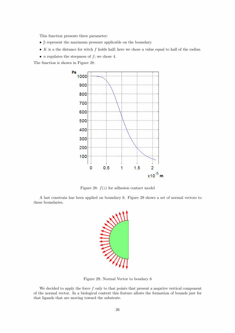
This function presents three parameter:

• β represent the maximum pressure applicable on the boundary.

• K is a the distance for witch f holds half; here we chose a value equal to half of the radius.

• n regulates the steepness of f ; we chose 4.

The function is shown in Figure 28.

Figure 28: f(z) for adhesion contact model

A last constrain has been applied on boundary 6. Figure 29 shows a set of normal vectors tothese boundaries.

Figure 29: Normal Vector to boudary 6

We decided to apply the force f only to that points that present a negative vertical componentof the normal vector. In a biological context this feature allows the formation of bounds just forthat ligands that are moving toward the substrate.

26

The mesh that we used is formed by triangular elements of 1.5 µm size, Figure 30 shows it.

Figure 30: Mesh for adhesion contact model (dimension in µm)

Figure 31 shows the vertical displacement at steady state for increasing values of β (1060, 2060,3060, 4060).

27

Figure 31: Diplacement in z direction for adhesion contact model for β values of 1060, 2060, 3060and 4060, rigid substrate without nucleus (dimension in µm)

We can see that the stronger is the force the more the cell attaches to the substrate.We haven’t considered so far the presence of the nucleus. The nucleus has a strong influence on

the mechanical behaviour of the cell, and therefore has to be considered. According to Maniotisat al. (1997), the nucleus is about 10 times stiffer than the cytoplasm. To model it we still adoptneo-Hookean equation.

The geometry of the system is presented in Figure 32.

28

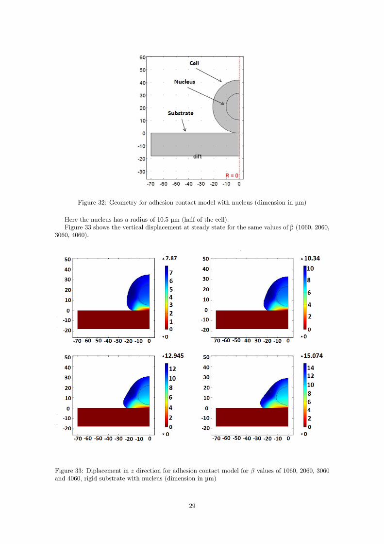
Figure 32: Geometry for adhesion contact model with nucleus (dimension in µm)

Here the nucleus has a radius of 10.5 µm (half of the cell).Figure 33 shows the vertical displacement at steady state for the same values of β (1060, 2060,

3060, 4060).

Figure 33: Diplacement in z direction for adhesion contact model for β values of 1060, 2060, 3060and 4060, rigid substrate with nucleus (dimension in µm)

29

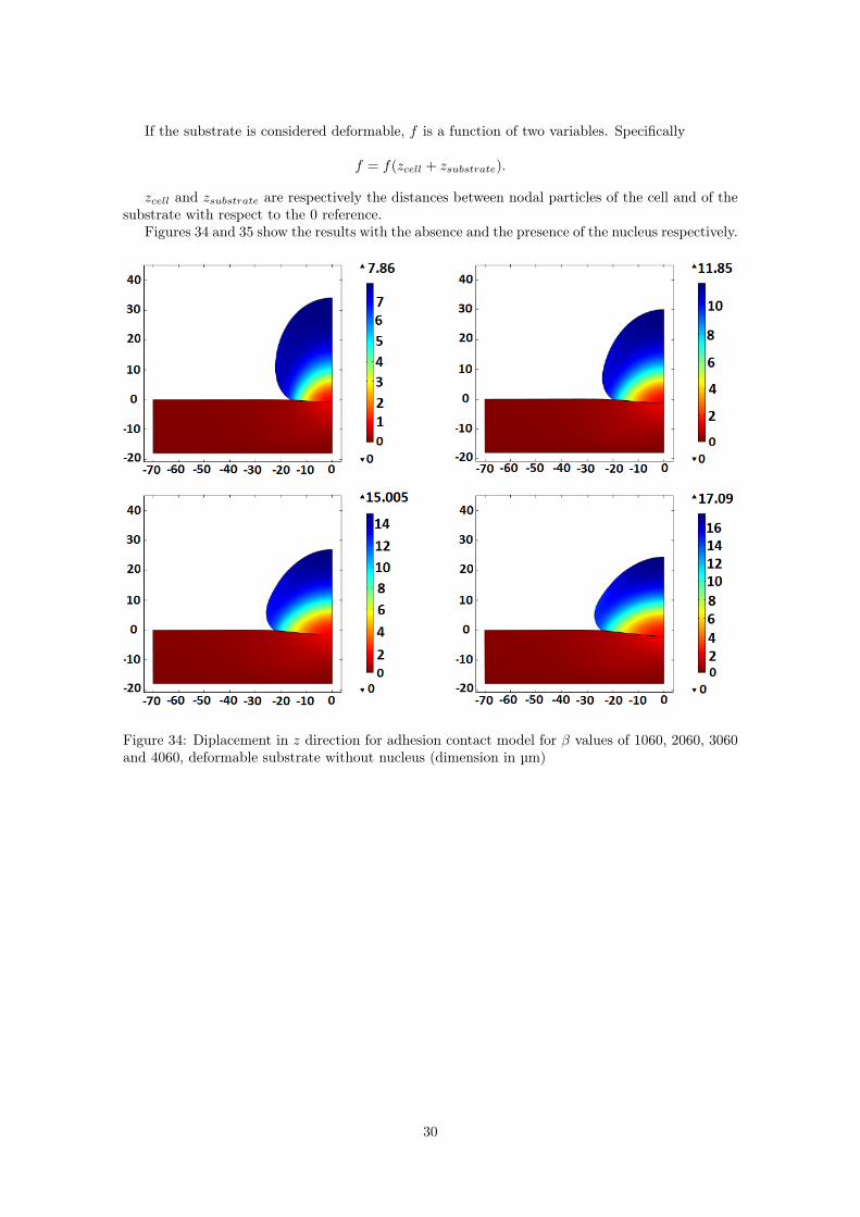
If the substrate is considered deformable, f is a function of two variables. Specifically

f = f(zcell + zsubstrate).

zcell and zsubstrate are respectively the distances between nodal particles of the cell and of thesubstrate with respect to the 0 reference.

Figures 34 and 35 show the results with the absence and the presence of the nucleus respectively.

Figure 34: Diplacement in z direction for adhesion contact model for β values of 1060, 2060, 3060and 4060, deformable substrate without nucleus (dimension in µm)

30

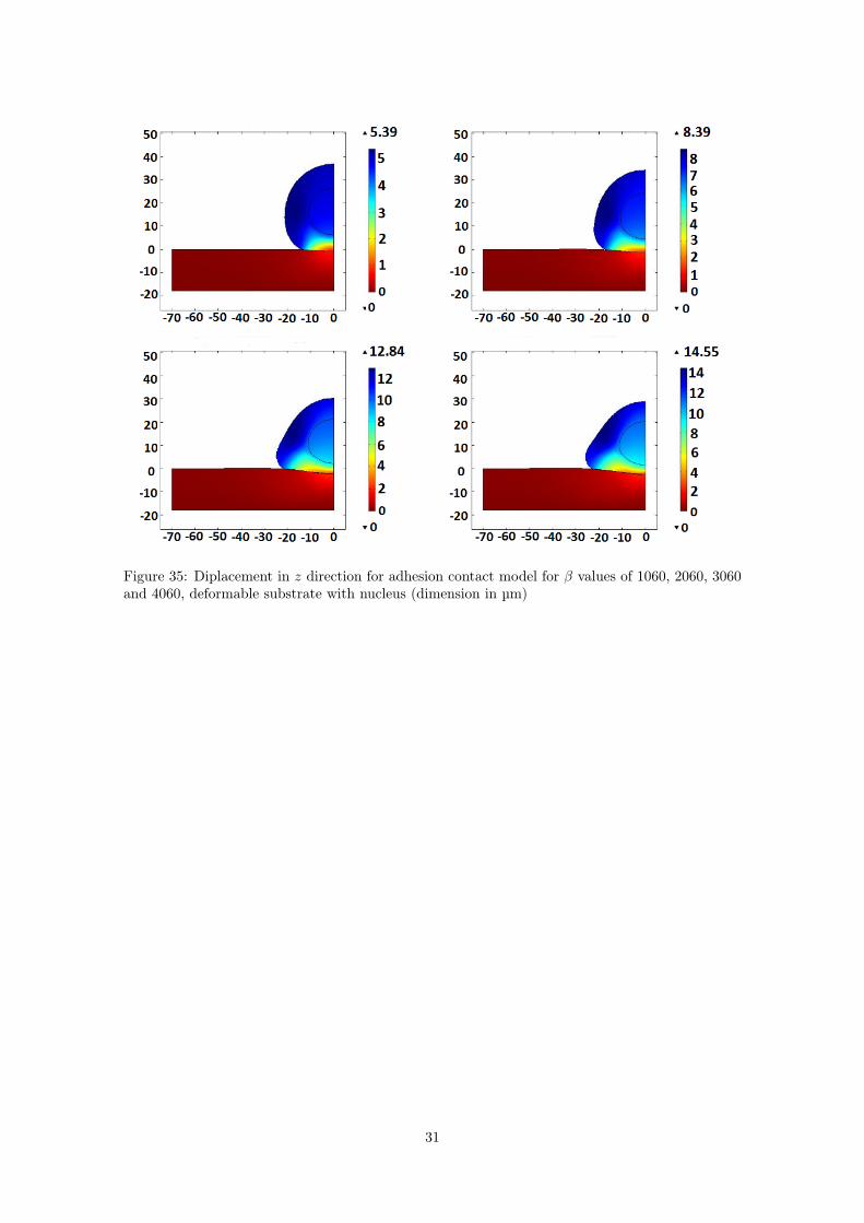
Figure 35: Diplacement in z direction for adhesion contact model for β values of 1060, 2060, 3060and 4060, deformable substrate with nucleus (dimension in µm)

31

Part VI

Simulation of adhesive contact process withAFM indentationThe first model developed in this thesis aims to simulate AFM; basically we recorded the reactionforce of the complex cell-substrate while indenting. It happens, however, that fibroblasts arealready prestressed before measuring force-deformation profiles. This is due to complex biochemicalinteractions that rise between ligands and receptors. In the second model, we simulated this processby defining a certain boundary pressure and observing how the geometry reaches the steady stateconfiguration.

The last simulation aims to perform AFM with a system that is already prestressed. In orderto do that we simulated AFM using, as initial condition, the solution obtained in the secondsimulation.

This model considers the substrate always deformable. We used as initial conditions:

• the solution obtained from the second model ignoring the nucleus.

• the solution obtained from the second model considering the nucleus.

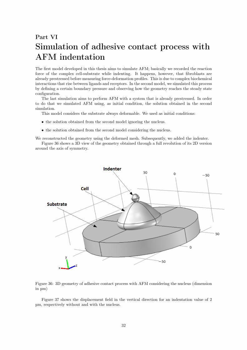
We reconstructed the geometry using the deformed mesh. Subsequently, we added the indenter.Figure 36 shows a 3D view of the geometry obtained through a full revolution of its 2D version

around the axis of symmetry.

Figure 36: 3D geometry of adhesive contact process with AFM considering the nucleus (dimensionin µm)

Figure 37 shows the displacement field in the vertical direction for an indentation value of 2µm, respectively without and with the nucleus.

32

Figure 37: Diplacement in z direction predicted by AFM 2D model for an indentation values of 2µm respectively without and with nucleus (dimension in µm)

Figure 38 shows the reaction forces ignoring and considering the presence of the nucleus re-spectively in blue and in red.

Figure 38: Reaction forces versus indentation predicted by the AFM 2D model without and withnucleus

33

Part VII

Conclusion and future works

This master thesis, carried out at the department of Solid Mechanics at Royal Institute ofTechnology (Stockholm, January-June 2011), aimed the investigation of mechanical properties offibroblasts through numerical modeling. AFM can be considered as the best tool in performingforce-deformation tests in order to get mechanical information from biological samples. Thereforethe principles of continuum mechanics directly applied to model these problems is the vanguard ofresearch in biomaterials.

Unfortunately, not a lot has been done so far and this study with its results have to be consideredpreliminary in this way.

This work builds up three numerical models of AFM in order to get force-deformation profilesthat want to be (in line of principle) identical to that ones that a normal operator can measure ina laboratory.

The complexity of the problem would bring the need of creating a strongly non-linear modelwith a numerous number of constants. On the other hand, our inability to perform measurementswith a real working machine, have forced us to use the simplest between the family of non-linearmodels (neo-Hookean equations).

Even though a neo-Hookean material cannot describe the recorded strong non linearity of theAFM response, our first minimal model predicts forces of the same order of magnitude (Figure16). Furthermore, when moving the position of the indenter along the cell surface, we showed theamount of changes of the global response (Figure 24).

As we said in the introduction, it happens that, due to the establishment of complex biochem-ical interactions between cell and substrate, the system is already prestressed before indenting.Therefore, the subsequent response will depend also on this process of attachment.

The second model aims on simulating this phenomenon. However, for simplicity, we did’t modelthe real interaction between proteins and ligands that depends of course on numerous factor (howmany proteins, which kind, their spacial distribution, the force of each bound ...), but we preferedto replace all this phenomena with a boundary pressure applied on the cell’s surface (Figure 28).How this pressure actually looks like is unknown. To model it, we chose an Hill function, but anyother decreasing function of the radius could have fit.

Anyway, the result obtained is still interesting: the bigger indeed the Hill function, the strongerthe process of attachment is. Also, the simulations showed how the substrate deformability hasa minor impact on the final results and how the shape of the cell changes non considering orconsidering the nucleus respectively.

The last simulation unifies the assumptions of the previous two models. Basically we performedAFM on the system that is already prestressed. Here, we showed how the presence of the nucleusstrongly increases the AFM reaction force when the average deformation ε becomes big.

As we mentioned, this preliminary work has to be integrated with the possibility of using a realmachine. In this context indeed we could study: the implications of a visco-hyperelastic model, atime dependent solver, how the mechanical response is influenced by the mechanical properties ofthe substrate, anisotropy et cetera.

34

References

[1]A. F. Bower (2009), Applied Mechanics of Solids, United States of America, CRC Press.

[2] David Boal (2002), Mechanics of the cell, New York, Cambridge University Press.

[3] K.S. Birdi (2003), Scanning probe microscopes, Florida, CRC Press.

[4] X. Zeng, Shaofan Li (2011), “Multiscale modeling and simulations of soft adhesion and contactof stem cells”, Journal of Mechanic behavior of biomedical materials, pp 180 - 189.

[5] H. Huang, R. D. Kamm, R. T. Lee (2004), “Cell mechanics and mechanotrasduction:pathways, probes, and physiology”, Am J Physiol Cell Physiol 287: C1-C11.

[6] T. G. Kuznetsova, M. N. Starodubtseva, N. I. Yegorenkov, S. A. Chizhik, R. I. Zhdanov(2007), “Atomic force microscopy probing of cell elasticity”, Micron 38, pp 824 - 833.

[7] J.P. McGarry, B.P. Murphy, P.E. McHugh (2005), “Computational mechanics modelling ofcell-substrate contact during cyclic substrate deformation”, Journal of the mechanics andphysincs of solids 53, pp 2597 - 2637.

[8] V. Lulevich, H. Yang, R. Rivkah Isseroff, G. Liu (2010), “Single cell mechanics of keratinocytecells”, Ultramicroscopy 110, pp 1435 - 1442.

[9] K. A. Beningo, C. Lo, Y. Wang (2002), “Flexible Polyacrylamide Substrata for the Analysis ofMechanical Interactions at Cell-Substratum Adhesion”, Methods in cell biology 69, chapter 16.

[10] M. Sato, K. Nagayama, N. Kataoka, M. Sasaki, K. Hane (2000), “Local mechanicalproperties measured by atomic force microscopy for cultured bovine endothelian cells exposed toshear stress”, Journal of Biomecjanics 33 , pp 127-135.