biomechanical analysis of sport performance of...
TRANSCRIPT

UNIVERSITÀ DEGLI STUDI DI PADOVA
Corso di Laurea Magistrale in Bioingegneria
Biomechanical analysis of sport performance
of Wheelchair Rugby
Italian National Team players
ANNO ACCADEMICO 2015/2016
Tesi di laurea di: Maria Laura Magrini
Dipartimento di Ingegneria dell’Informazione
Relatore: Prof. Nicola Petrone
Dipartimento di Ingegneria Industriale

1
Summary
ABSTRACT ............................................................................................................................... 5
INTRODUTCION ...................................................................................................................... 7
CHAPTER 1 Wheelchair Rugby .............................................................................................. 9
1.1 Classification .............................................................................................................. 9
1.2 On court rules .......................................................................................................... 10
1.3 Wheelchairs ............................................................................................................. 12
1.4 Athlete equipment ................................................................................................... 14
CHAPTER 2 Project: “Improvement of the residual neuromuscular capacities
in Wheelchair Rugby athletes” ............................................................................................. 17
2.1 Partners .................................................................................................................... 17
2.2 Aims of the project ................................................................................................... 18
2.3 Participants .............................................................................................................. 19
2.4 Diary of the project .................................................................................................. 20
2.5 Aims of this work and next developments .............................................................. 21
CHAPTER 3 Wheelchair propulsion: references ................................................................ 23
3.1 The wheelchair user shoulder: anatomy and problems .......................................... 23
3.2 Basis of wheelchair propulsion ................................................................................ 25
3.3 Mechanical efficiency............................................................................................... 27
3.4 Moments and forces at the handrim ....................................................................... 27
3.4.1 Moments and forces measuring ....................................................................... 28
3.4.2 Effective vs actual force at the handrim ........................................................... 29
3.4.3 Moments at the handrim in static propulsion: a study .................................... 31
3.4.4 Moments in dynamic and static propulsion ...................................................... 33
3.5 Inertial contributes in dynamic propulsion .............................................................. 35
3.5.1 Forward acceleration ........................................................................................ 35
3.5.2 Trunk Kinematics ............................................................................................... 36
3.5.3 The importance of the recovery time ............................................................... 36
CHAPTER 4 Project activity 1: isometric tests .................................................................... 39
4.1 Instrumentation ....................................................................................................... 39
4.2 Methods ................................................................................................................... 40
4.2.1 Tests description ............................................................................................... 40
4.2.1.1 Push forward ............................................................................................. 41

2
4.2.1.2 Shoulder flexion-extension ........................................................................ 41
4.2.1.3 Elbow flexion-extension ............................................................................. 43
4.2.2 Acquisition protocol ........................................................................................... 44
4.5 Data analysis ............................................................................................................. 44
4.3 Results ....................................................................................................................... 45
CHAPTER 5 Project activity 2: dynamic tests ...................................................................... 55
5.1 Instrumentation ..................................................................................................... 55
5.1.1 MEMS inertial sensors ....................................................................................... 55
5.1.1.1 MEMS Accelerometers ............................................................................... 56
5.1.1.2 MEMS Gyroscopes ..................................................................................... 58
5.1.2 Xsens technology ............................................................................................... 58
5.1.2.1 Xsens system of orientation ....................................................................... 60
5.1.3 Sensor fixation ................................................................................................... 62
5.1.3.1 Wheelchair frame sensor ........................................................................... 62
5.1.3.2 Wheel sensors ............................................................................................ 64
5.3 Methods .................................................................................................................... 65
5.3.1 Tests description ................................................................................................ 65
5.3.1.1 20 m sprint ................................................................................................. 65
5.3.1.2 Rotation ...................................................................................................... 66
5.3.1.3 Eight track .................................................................................................. 66
5.3.1.4 Match ......................................................................................................... 67
5.3.1.5 Friction ....................................................................................................... 68
5.3.2 Signal analysis .................................................................................................... 68
5.3.2.1 Frame sensor .............................................................................................. 69
5.3.2.2 Wheel sensors ............................................................................................ 74
5.3.2.3 Pre-elaboration .......................................................................................... 76
5.3.2.4 Data analysis of 20 m sprint ....................................................................... 77
5.3.2.5 Data analysis of Rotation ........................................................................... 79
5.3.2.6 Data analysis of 8 Track .............................................................................. 80
5.3.2.7 Data analysis of a match ............................................................................ 85
5.4 Results ....................................................................................................................... 88
5.4.1 Push shape ......................................................................................................... 88
3
5.4.2 Push frequency .................................................................................................. 91
5.4.3 Dynamic tests .................................................................................................... 93
5.4.4 Dynamic Vs isometric force values ................................................................... 99
5.4.5 Match .............................................................................................................. 101
CHAPTER 6 Project activity 3: pressure tests ................................................................... 105
6.1 Instrumentation ..................................................................................................... 105
6.1.1 mFlex pressure mat ......................................................................................... 105
6.1.2 Mat placement ................................................................................................ 106
6.2 Methods .............................................................................................................. 107
6.2.1 Tests description ............................................................................................. 107
6.2.1.1 Static tests ............................................................................................... 107
6.2.1.2 Dynamic tests .......................................................................................... 108
6.2.2 Data analysis.................................................................................................... 108
6.3 Results .................................................................................................................... 109
CHAPTER 7 ...................................................................................................................... 115
7.1 Conclusions ............................................................................................................ 115
7.2 Future developments ............................................................................................. 115
REFERENCES ........................................................................................................................ 117
APPENDIX 1 ......................................................................................................................... 121
Power Spectral Density ................................................................................................... 121
APPENDIX 2 ......................................................................................................................... 123
Matlab code .................................................................................................................... 123
2.1 Peak detection for forward acceleration analysis............................................... 123
2.2 Covered distance ................................................................................................ 125
RINGRAZIAMENTI ............................................................................................................... 129

4

5
ABSTRACT
A project with the aim of assessing how Wheelchair Rugby can improve neuromuscular
activity of disabled people, was started in Padova in October 2015, with the participation of
Italian National Team players. Within its 2 years duration, an engineering, medical and
sportive group evaluates biomechanical, medical and sport training aspects to improve
players’ sport performance on court, with personal training and therapeutic programs which
give advantages also in daily activities. The present work describes the biomechanical
analysis performed on 19 players. The investigation of maximal isometric force in unilateral
and bilateral pushing forward and shoulder/elbow flexion/extension allowed assessing the
presence of asymmetries in contralateral joints, and determine force rankings of athletes.
Tests of sprint, rotation, eight track, and the analysis of a match assessed their ability in
dynamic sport performance. Pressure tests on the wheelchair seats allowed identifying the
presence of incorrect postures.

6
7
INTRODUTCION
Sport has many powers: it gives the chance to express personal abilities, meet new
people, fight for the same goal together, and go beyond physical and mental limits. For
people with physical impairments, caused by an accident or a disease, sport becomes even
more: a challenge with themselves, a need, a mean to overcome their limits, to acquire a
deeper knowledge of their body, able to help them also in daily life.
In this contest, Wheelchair Rugby was born as a Paralympic sport for people with
spinal cord injuries or with impairments that can be associated to tetraplegia. Started from
Canada in the late 70s, it spread all over the world, reaching Italy in 2011. A group of
enthusiastic people started to believe in this sport and to spread it, bringing to the
foundation of different sportive association and teams, from which the Italian National
Team was born.
After some years of training, national and European competitions, in October 2015 a
project aimed at acquiring a deeper knowledge of this sport, was started in Padova, with
the participation of some athletes of the Wheelchair Rugby Italian Team. The aim of this
ambitious project is to observe the Wheelchair Rugby athlete on his totality, in order to
improve his performance by bringing him to exploit at best his abilities.
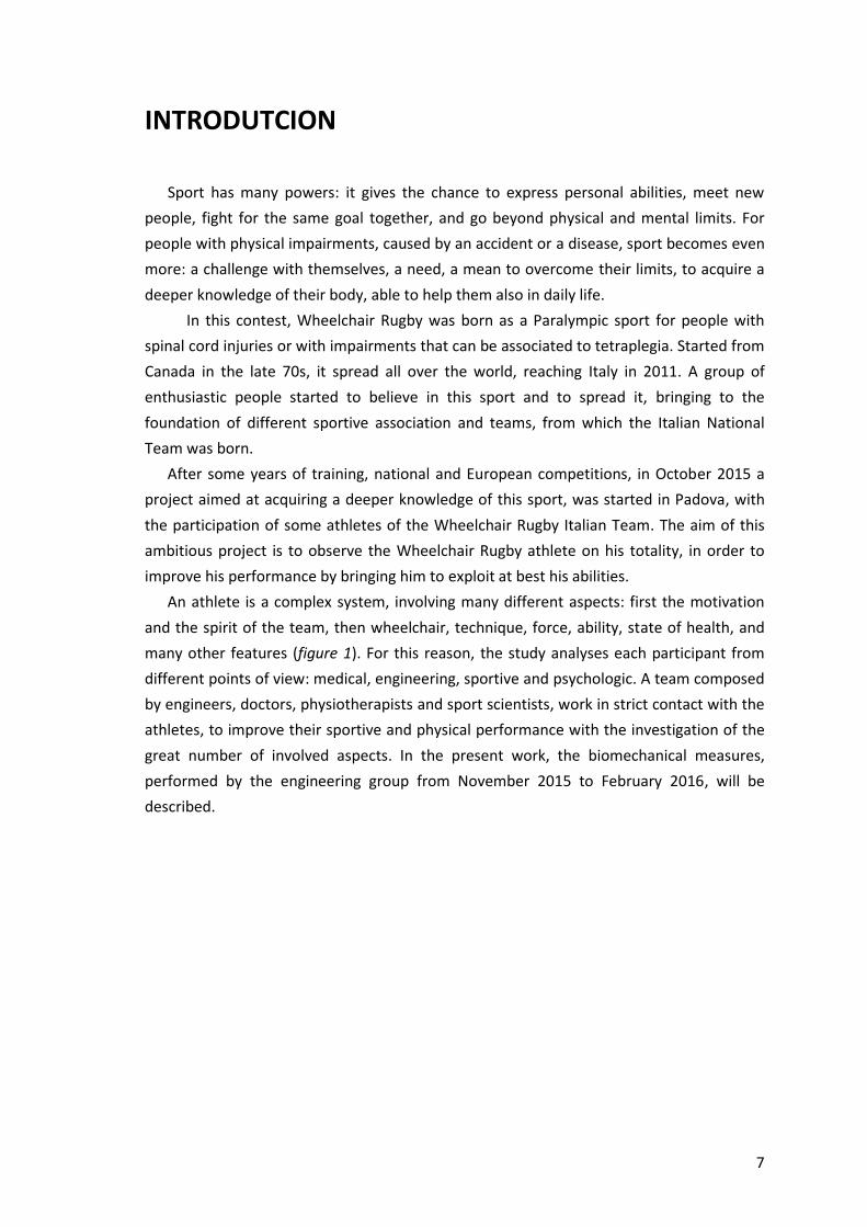
An athlete is a complex system, involving many different aspects: first the motivation
and the spirit of the team, then wheelchair, technique, force, ability, state of health, and
many other features (figure 1). For this reason, the study analyses each participant from
different points of view: medical, engineering, sportive and psychologic. A team composed
by engineers, doctors, physiotherapists and sport scientists, work in strict contact with the
athletes, to improve their sportive and physical performance with the investigation of the
great number of involved aspects. In the present work, the biomechanical measures,
performed by the engineering group from November 2015 to February 2016, will be
described.

8
Figure 1. Wheelchair Rugby athlete is a system involving many different aspects.

9
CHAPTER 1
Wheelchair Rugby
Wheelchair Rugby was born in Canada in 1977: it developed as a Paralympic sport
for people with tetraplegia. It grown intensively during the following years, and after being
presented as a demonstration sport at the Atlanta 1996 Paralympic Games, it finally made
its debut as a medal sport at the Sydney 2000 Paralympic Games. The sport is now practiced
in more than 25 different countries all over the world, and includes men and women on the
same team.
Wheelchair Rugby was first conceived for athletes with spinal cord injury: however,
in the following years, people with a wide variety of impairments started competing in this
sport. For this reason, a system of classification has the task of dividing roles within the
game, by taking into account physical and psychological features of the athletes, together
with their performance on court. In this chapter, the system of classification will be
described, together with the Wheelchair Rugby court, rules and wheelchairs features and
specifications.
1.1 Classification
Classification in Paralympic sport exists since the mid-1940s. Early classification was
based only on medical diagnoses, such as spinal cord injury, amputation or other neurologic
or orthopaedic conditions, conferring each athlete a sport class. However, recent reviews
have taken into account a more functional classification, determining the sport class not
only by health condition, but also by the relevance of an athlete’s impairment to carry out
fundamental activities to sport performance.
In the beginning of Wheelchair Rugby, according to its classification rules, athletes were
divided into three sport classes, largely determined by medical diagnosis and neurological
level of spinal cord injury. In 1991 a sport-focused classification system for Wheelchair
Rugby was started. Although the spinal cord injury examination was used as a guideline in
classifying the physical assessment, the classification rules were expanded to include, in the
determination of the sport class, fundamental activities of Wheelchair Rugby. This change
was made, on the other hands, to accommodate the growing number of athletes with
different disabilities from spinal cord injury. People with diseases as poliomyelitis, cerebral
palsy, muscular dystrophy, multiple sclerosis, multiple amputations and other conditions

10
with impairment in muscle strength similar to tetraplegia, started to be classified and
compete in Wheelchair Rugby.
Classification is a continuous updating progress: the last review of the classification
rules, by the International Wheelchair Rugby Federation (IWRF), dates to February 2015. All
athletes are under regular observation by classifiers, to ensure two important goals:
1. to determine eligibility to competition;
2. to divide athletes into classes, assigning them a point (0.5, 1.0, 1.5,…3.5). The highest
point values are given to players with the least movement restrictions. The lowest
point are assigned to those players with the most severe impairments.
People who want to compete in Wheelchair Rugby have to perform different tests and
evaluations, to determine the point of classification:
1. physical assessment by bench test;
2. technical assessment, including a range of sport specific tests and novel non-sport
tests;
3. observation assessment, consisting of observation of sport-specific activities on
court.
A system of classification is necessary both for the athlete and for the team: the assigned
point often determines the role of the athlete on court and the type of wheelchair he uses;
moreover, according to Wheelchair Rugby rules, the classification point has to be taken into
account in the formation of the team playing on court [1].
1.2 On court rules
Wheelchair Rugby combines elements of rugby, basketball, football and ice hockey and
it is played indoor in a basketball court, with a soft-cover volleyball ball. Each team is
composed by 4 players and 8 substitutes. For each team, the sum of athletes’ classification
points playing on court cannot pass 8. During the match, each athlete is assigned a defensive
or offensive role.
The field of play is a 15 x 28 m (figure 2), marked by end and side lines and is divided into
two halves by the centre line on which the centre circle is also located. On the end lines two
cones mark the goal line. At a distance of 1.75 m from the end lines, the key areas are signed.
Only 3 defenders are allowed to remain inside these areas while no player is allowed to
remain in the opponent's key area for more than 10 seconds when their team is in
possession of the ball. On the sides of the court near the side lines penalty areas are marked
out.

11
Figure 2. Wheelchair rugby field.
The aim of the game is to score a goal by passing or touching the opponent’s goal line
with two wheels while holding the ball: the team with the highest score at the end of the
match, wins. A match is played in 4 quarters of 8 minutes each, with 1 minute break at the
end of the first and third quarter and a 5 minute break at the end of the second one. In the
case of a tie, 3 minutes extra time is provided. Each team is entitled to 4 time-outs of one
minute during the normal length of the game, and one time-out during extended time. If
not all the time-outs are used, they can be transferred to extra time.
The game starts in the centre circle of the court: a referee launches the ball vertically
between two opponent players. The remaining players take position outside the circle. The
ball can be carried, dribbled, passed or stolen in any way, avoiding physical contact between
athletes. When moving, players can hold the ball on their thighs, pass it to a team mate or
bounce it, but it must be bounced or passed at least once every 10 seconds. Moreover, the
team in possession of the ball must pass it to the other half of the court within 15 seconds.
After a goal, foul or time-out, the ball is brought back into the game from the end line (when
a goal is scored) or from the side lines.
Many unfair sportive behaviours are interrupted by the referees commanding the game.
An offensive foul is punished by the loss of the ball, while a defensive foul is punished with
one minute out of the game (in the penalty area). A player under the penalty of leaving the
game cannot substitute an injured player. Instead of the one-minute penalty, the referee
can award a penalty goal when a player is fouled while in possession of the ball and in
position to score a goal [2,3].

12
Finally, it is worth to remember that Wheelchair Rugby would not exist without the great
number of people that help athletes in their primary necessities, inside and outside the
game: referees, staff members and volunteers.
1.3 Wheelchairs
The wheelchair is considered part of the player. It is the mean to move ad to express the
athletes’ specific talents and abilities within the game. At a first sight, it is possible to identify
two types of chair: offensive and defensive, as shown in figure 3. Nevertheless, the chair
does not automatically determine the role of the athlete during the match.
Figure 3. Offcarr Go Try Rugby Wheelchair. Left: Offensive chair; right: defensive chair.
An offensive chair is set up for speed and mobility, and equipped with a front bumper
and wings to prevent other wheelchairs from hooking it. In most cases, players with higher
points (more than 2.0) use this type of chair. Defensive wheelchairs contain bumpers set up
to hook and hold opponents players. These wheelchairs are most often used by players with
lower points (less than 1.5).
According to the sport rules, wheelchairs must meet some specifications, for reasons
of equality and safety: the athlete is responsible of respecting them. The player who does
not meet these specifications, is automatically banned from the game, until he returns on
the established standards. The main specifications coming from IWRF Rugby International
Rules are reported as follows.
Wheels: the wheelchair shall have four wheels.
o Two large wheels at the back (main wheels), used to propel the wheelchair;
their maximum diameter shall be 70cm (figure 4a). Each main wheel must
be fitted with a spoke guard protecting the area of contact by another

13
wheelchair, and a push rim. There shall be no bars or plates extending
around the main wheels. The rearmost part of the main wheel shall be
considered the back of the wheelchair and nothing can extend past this
point.
o Two small wheels at the front (casters): they must be on separate axles
positioned a minimum of 20 cm apart, measured centre to centre. The
housing that holds the caster must be positioned no more than 2.5 cm away
from the main frame of the wheelchair, measured from the inside edge of
the housing to the outside edge of the mainframe.
Anti-tip devices: the wheelchair shall be fitted with an anti-tip device attached at
the rear of the wheelchair, consisting in two wheels a minimum of 40 cm apart. If
the wheels of the anti-tip device are fixed, they cannot project further to the rear
than the rearmost point of the main wheels. The bottom of the wheels of the anti-
tip device must be no more than 2 cm above the floor (figure 4b).
Width: there is no maximum width; no point on the wheelchair may extend in width
beyond the widest point of the push rims.
Length: the length of the wheelchair, as measured from the front-most part of the
main wheel to the front-most part of the wheelchair, cannot exceed 46 cm (figure
4b).
Height: the height of the wheelchair, as measured from the floor to the midpoint of
the seat side rail tubing halfway between the front and back of the side rail, cannot
exceed 53 cm (figure 4b).
Other specifications, not reported in this work, refer to bumpers, wings and other
general standards about comfort and safety. Considering this rules, the athlete can
make personal adjustments, in order to satisfy his/her physical and functional needs [3].

14
Figure 4. a) Front view.
Figure 4. b) Side view.
1.4 Athlete equipment
Since wheelchair manoeuvrability is essential to guarantee the best performance on
court, players are provided with a specific equipment ensuring safety, comfort and
functionality during the game:
gloves: mostly covered with rubber on the palm and taped to the wrist, they create
additional grip in pushing, starting and stopping, and prevent skin injuries.
Sometimes they can also help compensating the loss of hand and finger function
associated with the particular disability of the athlete.
Straps: athletes are firmly strapped to the wheelchair frame to improve their
stability and balance. The three common strapped areas are the trunk, to eventually
15
compensate the lack of trunk control and to prevent the risk of falling forward during
a high strike; the thighs, to prevent shifting from the seat; the feet for a more
comfortable position.
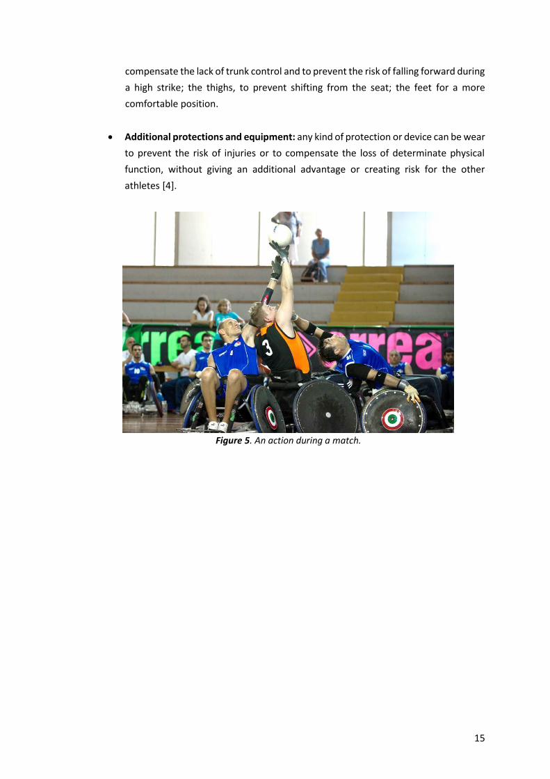
Additional protections and equipment: any kind of protection or device can be wear
to prevent the risk of injuries or to compensate the loss of determinate physical
function, without giving an additional advantage or creating risk for the other
athletes [4].
Figure 5. An action during a match.

16
17
CHAPTER 2
Project: “Improvement of the residual
neuromuscular capacities in Wheelchair Rugby
athletes”
In October 2015 a scientific project started in Padova, with the aim to assess how
Wheelchair Rugby can improve the residual neuromuscular capacities in people with
different physical disabilities. A scientific team composed by engineers, doctors,
physiotherapists and motor scientists collaborates with the Italian Wheelchair Rugby
National Team to perform physical, sportive and metabolic measures, in order to get
information about their physical state from a medical and biomechanical point of view.
These measures are collected to enhance their sportive performance, with the final goal of
entering in the international rankings and participate to the Paralympic Games (Tokyo
2020).
2.1 Partners
Several partners finance and support the project:
HPNR (Human Potential Network Research Onlus Via Toblino 53, Padova) the
proposer company, managing the financial and organizational aspects;
Industrial Engineering department (DIM) of University of Padova;
Physiology department of University of Padova;
FISPES (Italian Federation for Paralympic and Experimental Sports) providing a
representation of the Wheelchair Rugby Italian National Team and its supporting
staff;
Offcarr SRL (Via dell’Artigianato 29, Villa del Conte, Padova), the main provider of
Italian rugby wheelchairs, also interested in the investigation of biomechanical
properties of movement and posture, and on the improvement of the structural
frame of wheelchairs.
OIC foundation (Opera Immacolata Concezione, via Toblino 53, Padova), providing
the structures, and the equipment for the athletic preparation.
Microgate (Via Stradivari 4, Bolzano) providing instruments for the biomechanical
study;
18
Tecnogym (Via Calcinaro 2861, Cesena, FC) providing instruments for the personal
training;
DJO Italia SRL (Via Leonardo da Vinci 97, Trezzano sul Naviglio MI)
CIP (Italian Paralympic Committee).
2.2 Aims of the project
The project has a 2 years duration (from October 2015) and within this time, there are
three main goals that it aims to achieve:
improving the motor-functional sportive abilities of Wheelchair Rugby athletes,
trying to promote at best their residual capacities;
identifying individual rehabilitation programs;
producing scientific protocols in order to classify athletes and supervise their
performances during the rehabilitation programs.
Once the project is concluded, the results will be used with spinal unities and other
related associations, in order to exploit at best the collected information. The results may
be extended for other sports for people with disabilities. Moreover, two or more official
classifiers, formed during the project duration, may work together with FISPES and IWRF
(International Wheelchair Rugby Federation). Finally, the project may bring to the creation
of an Italian reference centre for study and training of Paralympic sports, in the University
of Padova, with an official role given by CIP.
The project aims at an evaluation of players under different points of view:
biomechanical, medical and physiological investigations are able to create a general
overview of the athletes. A sport engineering research group works for biomechanical
measures, a group of doctors and physiotherapists investigates different medical and
physiological aspects, and a sport medicine group works for the athletic training. In
particular, these aims are divided into three main aspects, described in the following lines.
Biomechanical evaluations.
1. Study of the athletic performance:
o measuring of dynamic forward push force and braking;
o measurement of the ability to spin;
o evaluation of the effectiveness in applying and sustain blocks;
o evaluation of the strength of delivering the ball.
2. Study of the properties of the wheelchair:
o road load measurement;
o maximum stress detection.

19
3. Study of posture and stability:
o pressure distribution on cushion;
o calculation of the 3D position of the center of gravity;
o calculation of stability indexes.
Medical evaluations.
1. Study of the metabolic consumption:
o measurement of the metabolic capacity thresholds;
o estimation of body composition;
o evaluation of muscle activation.
2. Study of joint mobility:
o ROM evaluation of shoulder joint;
o ultrasound detection of muscle structure in the shoulder.
Sport medicine evaluations.
1. Identification of individual training schemes:
o exercises during the team meetings;
o exercises to individually perform outside the team training;
2. Study of physiological variables:
o ability of isometric shoulder and elbow flexion/extension;
o measuring of VO2max in ergometer tests;
o measuring of RR and REE;
o measuring of lactate and ventilator threshold (IAT);
o recording of HR in different training situations;
o EMG recording for different muscle groups.
3. Study of an appropriate individual diet:
o Daily calories uptake related to individual consumption and
workloads.
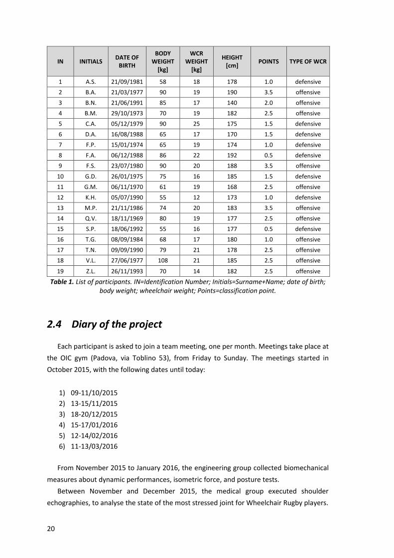
2.3 Participants
The participants are 19 male players, with different levels of training. They are part of the
Italian Wheelchair Rugby National Team, born in Padova in 2012. The list of players
participating in the project, with their anthropometric parameters, classification points and
type of wheelchair, is contained in the following table (1).
20
IN INITIALS DATE OF
BIRTH
BODY WEIGHT
[kg]
WCR WEIGHT
[kg]
HEIGHT [cm]
POINTS TYPE OF WCR
1 A.S. 21/09/1981 58 18 178 1.0 defensive
2 B.A. 21/03/1977 90 19 190 3.5 offensive
3 B.N. 21/06/1991 85 17 140 2.0 offensive
4 B.M. 29/10/1973 70 19 182 2.5 offensive
5 C.A. 05/12/1979 90 25 175 1.5 defensive
6 D.A. 16/08/1988 65 17 170 1.5 defensive
7 F.P. 15/01/1974 65 19 174 1.0 defensive
8 F.A. 06/12/1988 86 22 192 0.5 defensive
9 F.S. 23/07/1980 90 20 188 3.5 offensive
10 G.D. 26/01/1975 75 16 185 1.5 defensive
11 G.M. 06/11/1970 61 19 168 2.5 offensive
12 K.H. 05/07/1990 55 12 173 1.0 defensive
13 M.P. 21/11/1986 74 20 183 3.5 offensive
14 Q.V. 18/11/1969 80 19 177 2.5 offensive
15 S.P. 18/06/1992 55 16 177 0.5 defensive
16 T.G. 08/09/1984 68 17 180 1.0 offensive
17 T.N. 09/09/1990 79 21 178 2.5 offensive
18 V.L. 27/06/1977 108 21 185 2.5 offensive
19 Z.L. 26/11/1993 70 14 182 2.5 offensive
Table 1. List of participants. IN=Identification Number; Initials=Surname+Name; date of birth; body weight; wheelchair weight; Points=classification point.
2.4 Diary of the project
Each participant is asked to join a team meeting, one per month. Meetings take place at
the OIC gym (Padova, via Toblino 53), from Friday to Sunday. The meetings started in
October 2015, with the following dates until today:
1) 09-11/10/2015
2) 13-15/11/2015
3) 18-20/12/2015
4) 15-17/01/2016
5) 12-14/02/2016
6) 11-13/03/2016
From November 2015 to January 2016, the engineering group collected biomechanical
measures about dynamic performances, isometric force, and posture tests.
Between November and December 2015, the medical group executed shoulder
echographies, to analyse the state of the most stressed joint for Wheelchair Rugby players.

21
Starting from January 2016, a personal program of training was monthly given to the
athletes, with the aim of improving their muscular force and resistance; moreover, in
February 2016 a personal diet was produced and given to everybody.
Visceral and cardiocirculatory aspects are still under investigation, starting from
February 2106, through interviews and questionnaires about the personal habits of the
athletes sphincterical management during trainings and matches, and the use of standing
instruments at home.
From January to March 2016, metabolic tests were executed by the sport medicine
group, to evaluate the VO2 max of each athlete, durgin a test made on the ergometer.
In parallel, from February 2016, a study on the structure of wheelchair’s frame is under
investigation by the Engineering group.
2.5 Aims of this work and next developments
The project aims at achieving different goals along its two years duration: in this work,
the biomechanical results collected during the team meetings from November 2015 to
January 2016 are described. A study of Wheelchair Rugby player was carried out, to evaluate
their performance on court and their physical abilities. Firstly, with the use of a load cell, the
isometric force expressed in the fundamental movements involved in pushing a wheelchair,
was tested. With the use of inertial sensors, the athletes’ ability of accelerating, spinning
and braking was measured in different situations and during a match. Finally, a posture test
about the pressure acting on the chairs ‘seat was performed. The present paper describes
the protocols of acquisition, data analysis and the related results, collected by the
Engineering group. The outcome is a general overview of each player’s starting point, from
a biomechanical point of view.
Nowadays, athletes are undergoing a program of training, based on force improving and
compensation of missing abilities, a team training, and an educational program about diet
and management of their physiological needs. For this reason, in the following months, the
biomechanical measures described in this work will be execute again, to determine whether
there have been a physical and performance improvement or not. This is also a motivation
for athletes, who have to achieve a goal that can be measured quantitatively. Therefore,
starting from the first set of biomechanical measures, with the acquisition of time tests and
forces, and the use of rankings for each test, each athlete developed the awareness of his
points of strength and the aspects to enhance, also in relationship with the other mates.
This lead to a healthy competition, that could also serve as an additional motivation.

22
The work of the engineering group is still going on. With an Offcarr offensive wheelchair,
equipped with strain gauges, the main loads acting on the frame in the case of impacts and
during a match, are under measuring. Moreover, in the same conditions an accelerometer
at high frequency acquires the longitudinal acceleration. This will be the starting point for a
Finite Element Method analysis, with the aim of improving the structure of Rugby chairs
produced by Offcarr factory, and to make them more customized for the athlete’s specific
needs.

23
CHAPTER 3
Wheelchair propulsion: references
Wheelchair propulsion technique, in daily use as in sport, is determined by three basic
features:
I. the user (the motor) who produces energy and power for propulsion;
II. the wheelchair, which determines power requirements;
III. the wheelchair-user interaction, which determines the efficiency of power transfer
from the motor to the wheelchair.
The wheelchair-user connection is a system producing an amount of work, to win some
resistance forces: some studies demonstrated that the mechanical efficiency of this system
in the propulsion movement, is low. The contribution of biomechanics and physiology to the
understanding of these elements in improving the performance in wheelchair sports and
daily use is fundamental [5]. In the present chapter, a literature research of biomechanical
studies about wheelchair propulsion is reported.
3.1 The wheelchair user shoulder: anatomy and problems
The human arm is, contrary to the human leg, not specialized. Leg has very powerful
muscles to support the body weight, allowing walking, running, jumping, without a higher
range of movement. In contrast, arm has a large range of motion, and can perform many
different tasks, from manipulation of small objects to handling of heavy materials. From an
anatomical point of view, the functional difference between arms and legs is well visible in
the difference of structure between the shoulder joint (figure 6) and the pelvis.
The two main bones of the shoulder are the humerus and the scapula, which extends up
and around the shoulder joint to form the acromion and the coracoid process. The end of
the scapula, called the glenoid, meets the head of the humerus to form a glenohumeral
cavity that acts as a flexible ball-and-socket joint. Ligaments connect bones of the shoulder,
and tendons join the bones to the surrounding muscles. The biceps tendon attaches the
biceps muscle to the shoulder and helps to stabilize the joint.
Shoulder can perform movements of adduction, abduction, flexion, extension, internal
rotation, external rotation, and 360° circumduction in the sagittal plane. Furthermore, it
allows for scapular protraction, retraction, elevation, and depression. These free of
movement also makes the shoulder joint unstable.

24
Figure 6. Shoulder joint.
The loose connection of the scapula to the trunk is the main reason for the large range
of motion of the arm. Since the scapula is able to slide and rotate over the surface of the rib
cage, it is possible to move the base of the arm, the gleno-humeral joint (GH). This leads to
a high increase in the range of motion of the arm: making a comparison with the leg, in the
hips this is not allowed, since the pelvis does not have a range of movement as it is for the
scapula.
A second reason for the large range of motion of the arm is the fact that the GH joint is
shaped as a small and shallow cup (the glenoid) and a large saucer (the humeral head). The
cup and saucer are connected by strong, but loose ligamentous tissue. The joint structure
allows for rotation in three directions, as well as some translation. Despite the fact that the
GH joint is loose, spontaneous subluxation can occur: it is assumed that this is the result of
muscular control by the rotator cuff muscles. For this reason, a good coordination between
these muscles is fundamental.
People seated on a wheelchair use their arms as legs. Therefore, considering the features
of arms, high and cyclic loads are not anatomically favourable. Moreover, people competing
in wheelchair sports use their arm even more during training: heavier loads, more cycles,
higher velocity of movements. Therefore, athletes with an incomplete shoulder muscle
system, and for whom muscular control is limited, will be at risk regarding shoulder luxations
and other injuries[6]. Shoulder and wrist complaints are very common within the wheelchair
users: Campbell and Koris diagnosed 24 patients with a cervical spinal cord injury with acute

25
and chronic shoulder pain. Some publications state that at least 50% of the wheelchair users
suffer of wrist complaints. About 30-50% of this group has problems with their shoulders
[7]. In the present study, on 19 Wheelchair Rugby players, shoulder echographies revealed
an inflammation of the long head of biceps tendon in 17 of them, and a subacromial bursitis
in 18 of them.
The high prevalence of complaints of wheelchair-user is a clear indication that the
mechanical load in propulsion is unfavourably high. An explanation of this can be found in
the fact that additional muscular effort is needed for the stabilization of the shoulder
mechanism in movements that are not usual for the joint, especially for prevention of
shoulder luxations. These extra muscular forces would then lead to overload of one or more
of shoulder muscles, but also to high compression forces in the GH joint, which in turns
might lead to damage the joint cartilage. To a deeper understanding of how a wheelchair
user the shoulder works, wheelchair propulsion must be studied in its different aspects [5].
3.2 Basis of wheelchair propulsion
Some studies investigated the propulsion kinematic technique of a wheelchair, in
ordinary activities and for different kind of sports. Wheelchair propulsion is studied as a
cyclic movement: a given propelling motion is repeated over the time at a given frequency
(f), to generate a certain linear velocity (v). With a first approximation, a cycle of propulsion
can be divided into two phases, as shown on figure 7:
push phase: hand in contact with the rim, effective force production;
recovery phase: non propulsive phase, hand is not in contact with the rim since the
arm is preparing to restart the next push.
In each push of the wheel, the user produces an amount of work (W). The product of
push frequency (f) and work (W) gives the average external power output (Pout), according
to:
Pout= f·W
The work produced in each push constitutes the integral of the momentary torque (M)
applied by the hands to the handrim over a more or less fixed angular displacement (Q).
The above equation can be rewritten into:
Pout= f· ∑ 𝑀 ∙ 𝑑𝑄
where torque is the product of the bi-manual tangential force, which is applied on the
handrim, and the radius of the hand rim.

26
Figure 7. Representation of a wheelchair propulsion technique: HC=hand contact; HR=hand
release; PA=propulsion angle; SA=start angle; EA=end angle. [8]
Physiological measures (i.e. energy cost, physical strain) can be linked with
biomechanical measures (i.e. power output, work, force and torque production) to obtain a
general view of the force acting on the system. Considering wheelchair sports, the
wheelchair-user combination is approached as a free body that moves at a given speed (v)
and encounters the following resistance forces (Fdrag): rolling friction (Froll), air resistance
(Fair), internal friction (Fint) and the metabolic consumption of the user (Fmet). Power
production during wheelchair propulsion is achieved by upper body work, primarily the
arms. The forces (Fprop) acting to propel the system and winning the resistance are: inertial
force of the system in movement (Finert), the action produced by arms (Farm) and the push
force produced by the movement of the trunk (Ftrunk). In conclusion, the acting forces are:
Fdrag= Froll + Fair + Fint + Fmet
Fprop= Finert+ Farm+ Ftrunk
The output force is given by:
Fout= Fprop-Fdrag
The power output that must be produced by the system to maintain the velocity v is:
Pout=Fout ∙ v

27
Starting from this statements, it is possible to perform tests in order to obtain a quantitative
evaluation of the mechanical efficiency of the movement [5,8].
3.3 Mechanical efficiency
The relatively small muscle mass of the upper extremities and increased tendency for
local fatigue lead to a much lower maximal work capacity in comparison to leg work. Peak
oxygen uptake is usually 60-85% of that in leg work [9]. Measurement of power output in
wheelchair exercise testing, in combination with physiological measurements of the cardio-
respiratory strain, gives additional information on the physical capacity of the person, and
is also required for the calculation of the efficiency of the wheelchair-user system.
The gross mechanical efficiency (ME) is defined as the ratio between externally produced
energy (power output) and internally liberated energy (En) according to:
ME=(Pout/En)·100 (%)
Calculation of energy expenditure during submaximal exercise is based on the
measurement of oxygen uptake (VO2) and simultaneous respiratory exchange ratio (RER)
[36]. In the case of handrim propulsion on a wheelchair ergometer, the work done by the
upper limb muscles is easily calculated by the tangential force exerted by the subject on the
wheels to generate these rotations, usually converted to equivalent work (in W or kcal/min)
[10]. In handrim propulsion, ME appears up to 11–12% [11]; In arm crank ergometer, values
of ME around 15% are commonly found.
Although there are not many studies about mechanical efficiency in wheelchair
propulsion, it appears clear that the value is low: this may be explained by the small muscle
mass in comparison with legs, the complex functional anatomy of the upper extremity and
the composite movement of propulsion. As described before, the anatomy of arm and
shoulder, not specialized in movements involving repetitions, peaks of force and extreme
joint deflections, requires some extra work to stabilize the glenohumeral joint. Another
important feature is the way in which forces are applied to the hand rims, and the analysis
of the acceleration of the system: this can give an explanation of the low mechanical
efficiency, and address an effective pushing technique [5].
3.4 Moments and forces at the handrim
In wheelchair pushing, any force that has a tangential component respect to the wheels,
contributes to the propulsion. Forces in other directions do not directly give a contribute to

28
the forward movement. The studies reporting only tangential forces or moments about the
hub, do not take into account the components of the handrim forces. For this reason, a
three dimensional analysis of the force generation pattern at the handrim, is a prerequisite
to relate force application strategies to risk for injuries, and to understand how the
propulsion technique can be improved in order to obtain a better sportive performance [8].
3.4.1 Moments and forces measuring
The recording of force acting on the handrim during wheelchair propulsion needs the
use of an instrumented wheel; a novel instrument that allows this measures is the
Smartwheel®: a modified wheel, instrumented with a 3-beam system that allows the
determination of three dimensional forces and moments [12]. As the Smartwheel® can be
mounted on the individual’s own wheelchair, wheelchair-user interface and external
conditions can be simulated. The output of the Smartwheel® consists of forces and
moments in three dimensions, determined by a world coordinate frame. The force
components Fx ,Fy and Fz are defined as directed horizontally forwards, horizontally
outwards and vertically downwards, respectively, in a right-hand coordinate system (figure
8); they are combined to give the resultant force Ftot .
To relate the forces to the wheel, the coordinate frame can be rotated such that the
force components Fx and Fz represent, respectively, the tangential (Ft) and radial (Fr) force
components of the hand rim.
The tangential force component Ft is the only force component that contributes to the
forward motion of the wheel. The radial force component Fr, and the axial force component
Fy, create the friction necessary to allow Ft to be applied. The resultant force Ftot, which is
the total force applied to the hand rim, is mathematically calculated by taking the vector
sum of the 3 force components Fx, Fy and Fz [8].
Veeger et al. [13] also introduced a parameter called Fraction of the Effective Force (FEF),
as a measure for the effectiveness of force application. FEF is the ratio of the effective
propulsion moment measured at the wheel hub (Mhub) to the resultant force:
FEF = (Mhub/r) /Ftot ∙ 100 (%)
where r is the radius of the rear wheel.
Some studies analysed the wheelchair propulsion to find a reason why users statistically
choose a mechanically disadvantageous movement. An explanation can be found in
biomechanics [8].

29
Figure 8. Coordinate frames on the instrumented wheel [8].
3.4.2 Effective vs actual force at the handrim
Since, during the push phase, the hands hold the rims, the movement of hands and arms
is considered as a guided circular movement. In guided movements, forces applied by the
hands do not directly influence the trajectory of the hands. As a consequence, it is possible
to apply a force that is not tangential to the hand rims.
Experimental results in which propulsion forces were measured with instrumented
wheels, showed that propulsion forces are indeed not tangentially directed. The direction
of the forces applied on the handrim does not agree with the most optimal direction in
terms of mechanical power production, i.e. the direction tangential to the handrims.
Surprisingly, this apparently, in mechanical terms, suboptimal direction of actual force
application was found for athletes as well as untrained subjects [13,14,15,16]. It appears
that this particular manner of force application is the most efficient force application
technique. In other words, subjects appear to adopt the technique that demands them the
30
least energy, given the mechanical constraints of the wheelchair-user combination [17]. The
reason why the users choose this force pattern can be found in the muscle contraction
during propulsion.
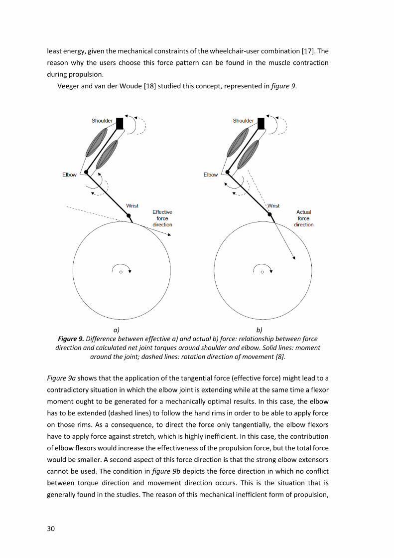
Veeger and van der Woude [18] studied this concept, represented in figure 9.
a) b) Figure 9. Difference between effective a) and actual b) force: relationship between force
direction and calculated net joint torques around shoulder and elbow. Solid lines: moment around the joint; dashed lines: rotation direction of movement [8].
Figure 9a shows that the application of the tangential force (effective force) might lead to a
contradictory situation in which the elbow joint is extending while at the same time a flexor
moment ought to be generated for a mechanically optimal results. In this case, the elbow
has to be extended (dashed lines) to follow the hand rims in order to be able to apply force
on those rims. As a consequence, to direct the force only tangentially, the elbow flexors
have to apply force against stretch, which is highly inefficient. In this case, the contribution
of elbow flexors would increase the effectiveness of the propulsion force, but the total force
would be smaller. A second aspect of this force direction is that the strong elbow extensors
cannot be used. The condition in figure 9b depicts the force direction in which no conflict
between torque direction and movement direction occurs. This is the situation that is
generally found in the studies. The reason of this mechanical inefficient form of propulsion,

31
is based on fact that this is the most efficient solution for muscle biomechanics: the
production of negative power is prevented and the strong elbow extensors can be used [8].
3.4.3 Moments at the handrim in static propulsion: a study
Some studies measured, with an instrumented wheel, the moments at the rim in
wheelchair propulsion. A work by Lan-Yuen Go et al. [19] examined 5 male healthy subjects
(non wheelchair-users) during a maximal isometric wheelchair propulsion. The study
wanted to demonstrate that, given a subject specific profile of the strengths of each of the
upper extremity joints as a function of joint angle, there is an optimal direction of force
application in the handrim to maximize the propulsion moment about the wheel axle at
each instant of the propulsion cycle. In the experimental setting, the instrumented wheel
had a handrim radius of 25.4 cm, and was locked to prevent
the forward movement as the subjects pushed with
maximum isometric effort. Five hand positions,
corresponding to wheel angles θ of 120, 105, 90, 75 ,60°
(figure 10) were assigned in a random order.
The subjects performed four trials of maximal
wheelchair propulsion effort for each hand position.
Applied hand forces in the laboratory reference frame and
progression moments about the wheel axle were averaged
for the four repetitions to represent each subject’s
performance at each hand position. The force direction and magnitude of force applied to
the handrim were determined.
To estimate the joint strength in an isolated loading condition, the isometric shoulder
flexion and extension muscle strength were measured at different angles, using a
dynamometer. Muscle strength at each position were determined as the peak force
generated during a 3s contraction; three trials of muscle strength were collected.
The optimal force direction was determined at each instant with a linear optimization
problem which aims to maximize the moment about the wheel axis, M0, considering the
constraints of the subject’s shoulder and elbow joint moment-generation capabilities for
the specified joint angles. The results are represented in the following figures (11,12,13).
Figure 10. Definition of angle θ and Top Dead Centre (TDC)

32
Figure 11. Moment of elbow and shoulder flexion/extension during isometric contractions [19].
Figure 12. Mean and standard deviation of handrim force in the horizontal (left) and vertical
(right) directions [19].

33
Figure 13. Mean and standart deviation of progression moment ath the hand rim, at five hand positions [19].
The results revealed that the progression moment was greater at both initial and terminal
propulsion positions (wheel angles of 120° and 60° respectively) and smaller in the mid
propulsion position (wheel angle of 90°). The applied handrim force in the horizontal
direction, however, was smaller in the initial and terminal propulsion positions and larger
during mid-propulsion while the applied handrim force in the vertical direction showed a
bimodal pattern, negative prior to top dead centre (TDC) position. These vertical and
horizontal force directions correspond to a force which is radially away from the wheel axle
posterior to the TDC and radially toward the wheel axle anterior to TDC.
3.4.4 Moments in dynamic and static propulsion
The results described in the previous paragraph are an example of the data collected in
different studies of static propulsion. Nevertheless, they are in contrats with those
documented for dynamic tests: for example, the wheelchair user does not have to initiate
acceleration of the wheel at all hand positions as in the static equivalent.
During dynamic wheelchair propulsion, the progression moment reaches its maximum
value in mid-propulsion while in experimental models and static studies, the peak in the
progression moment is recorded at the beginning and terminal phases of the propulsion
cycle. The static analysis reveals that the hand position at TDC may not be optimal to for
the upper extremities to generate large forces in the handrim: since the applied handrim
force is sperimentally nearly perpendicular to the line from the hand to the shoulder, a large
shoulder moment will result. For example, in wheelchair racing, users always flex their trunk
anteriorly to propel the handrim with their hand anterior to TDC: this hand position allows
larger progression moments to be generated because their lever arms enable the upper
extremities to tolerate greater external loading.

34
Moreover, the force direction posterior to TDC found in static propulsion, differs greatly
from the results of dynamic wheelchair propulsion. The direction of handrim force during
dynamic wheelchair propulsion is toward the wheel axle during the whole propulsion phase,
including the period when the hand position is behind the TDC (figure 14).
Figure 14. Stick diagrams showing the position of the upper extremity during static and dynamic wheelchair propulsion. The force vector at the rim is shown [23].
To generate a push force directed away from the wheel axle, the elbow flexor must be
activated, and this would indeed be beneficial for propulsion as the elbow must flex during
this phase of the cycle (behind TDC). However, halfway through the propulsion phase, the
applied force must change to progress the wheel and so the elbow extensor needs to be
immediately activated at that point in the cycle. During static propulsion, switching from
elbow flexion to extension is not difficult, however, the change in muscle activation from
elbow flexor to elbow extensor dynamically may result in a more complex and inefficient
movement.
It could then be hypothesized that users could be trained through biofeedback to
activate their muscles more like that seeing during static analysis, to increase mechanical
efficency [19]. Nevertheless, care should be taken when using increasing FEF as a
rehabilitation goal, as higher FEF values shift handrim force contributions from muscles
crossing the elbow to those crossing the shoulder, which are already susceptible to overuse
injuries [20].
Considerable differences in force application during steady-state wheelchair propulsion
[21] and sprinting [22] have been demonstrated between people with quadriplegia and
those with paraplegia. The FEF in quadriplegics is the consequence of a significantly larger

35
inwards directed lateromedial force component (Fy). Friction at the hand rim is necessary
to produce the tangential component and can be generated through hand grasping, wrist
moment generation and/or directing the resultant force away from the tangential direction.
In quadriplegics without hand function, only the latter option is available. If triceps function
is limited, the generation of friction in a downward or outward direction is hampered.
Therefore, the inwards-directed lateromedial force component can serve as an effective
alternative for friction generation [8].
3.5 Inertial contributes in dynamic propulsion
The results found for static wheelchair propulsion differ from those recorded during
dynamic propulsion. For this reason, the research cannot limit to the study on moments and
forces at the handrim: the study of dynamic propulsion is necessary. Therefore, the
wheelchair-user system is moving: in this contest inertial events, not occurring in static
propulsion, highly contributes to the output performance.
3.5.1 Forward acceleration
Wheelchair propulsion under realistic conditions does not merely consist of an active
period (the push phase) and a passive period (the recovery phase), as commonly
described. It is composed by 3 phases, each with specific energy demands:
I. an acceleration phase caused by forces applied to the hand rims;
II. a second acceleration phase caused by the inertial forces acting on the wheelchair-
user system, caused by a backward arm and/or trunk-swing;
III. a deceleration phase during the second part of the recovery phase.
The deceleration is amplified because of inertial forces acting on the wheelchair-user
system, caused by an increased forward segmental velocity of the upper limbs to prepare
for the hand contact with the hand rims [8].
This fact finds a relevance in the study of forward acceleration of the wheelchair-user
system, collected with inertial sensors, in specific points of the wheelchair frame. The typical
forward acceleration trend is composed by high peaks of positive acceleration and high
peaks of negative acceleration: this is in line with the low mechanical efficiency found for
wheelchair propulsion. The acceleration trend gives other explanations about the
inefficiency of this system. This can be seen in the difference between experiments on the
ergometer and on real dynamic conditions. The acceleration on court is not directly
comparable to the acceleration on the ergometer, as on the court the mass of the
wheelchair-athlete system is accelerated, whereas on the ergometer only the moment of

36
inertia of the rotary parts has to be accelerated. Additionally, the breaking torque works
against acceleration and thus adds further resistance [24].
In stationary systems, inertial forces acting on the wheelchair, caused by accelerations
and decelerations of trunk and arms, are neglected. Vanlandewijck et al.[25] and Spaepen
et al. [26] showed that positive mechanical work during the recovery phase at velocities
higher than 1.67 m/sec can amount to one-third of the total mechanical work during the
propulsion cycle, because of inertial forces acting between the user and the wheelchair.
3.5.2 Trunk Kinematics The force is not only applied by arms: alterations in trunk inclination, if functionally
available, are most likely used as a force generation strategy. There are no biomechanical
studies specifically addressing the role of the trunk in hand rim wheelchair propulsion.
Nevertheless, trunk motion might be one of the most important force generating
mechanisms during fatigue, or high resistance wheeling, such as accelerating from standstill,
sprinting or uphill driving. Furthermore, trunk motion will directly affect rolling resistance
and air drag. In wheelchair sports classification procedures, trunk range of motion has been
determined as one of the key parameters in identifying the functional potential of
wheelchair sportsmen [8].
Some studies measured trunk excursions during manual wheelchair propulsion and
generally found a forward shift of the trunk as the amount of activity increases [27,28].
Vanlandewijck et al. [25] observed in 40 wheelchair athletes that the change from trunk
flexion to extension shifted significantly towards the end of the push phase when velocity
was increased from 1.11 to 2.22 m/s (from 68.39 to 93.15% of the PT) [29]. This might be
explained with the need of pushing with the hands more anteriorly on the handrim to exploit
a bigger lever arm, and with a higher push given by the trunk flexion.
3.5.3 The importance of the recovery time A number of studies have shown that a mere speed increase leads to a marked decrease
in propulsion cycle time (CT), mainly because of a decrease in propulsion time (PT) instead
of a decrease in recovery time (RT). The reason why RT, often qualified as a passive period,
remains almost constant as velocity increases, has been discussed by Vanlandewijck et al.
They investigated the propulsion technique in wheelchair basketball players, in different
velocities, at a constant power on a treadmill. The authors demonstrated that, in high
velocities, experienced wheelchair users adapt their propulsion technique not by changing
their style, but by increasing the amplitude of their movements. In fact, when propulsion

37
velocity increases, an increased backward arm swing is needed to generate a greater
acceleration of the hand before contact with the rim. Both the accelerated backward arm
swing and the preparation for hand contact result in an increased muscular activity. This
implies a higher muscle contraction velocity and is associated with an increased energy
expenditure and, consequently, a lower mechanical efficiency [8]. Decreased mechanical
efficiency can be explained by a significant change in the acceleration of the wheelchair-
user system during recovery time, caused by arm and trunk movements, inducing inertial
forces to act on the wheelchair. Consequently, mechanical work increased significantly
during the recovery phase. These findings indicate that studies on mechanical efficiency in
wheelchair propulsion should not only be focused on power supply during the push phase,
but also on the movement pattern during recovery [25].

38

39
CHAPTER 4
Project activity 1: isometric tests
In Wheelchair Rugby, as for all Paralympic sports played in a chair, arms are for athletes
their mean to express at best their abilities: the force they can exert with their arms
influences the pushing technique, the way of launching the ball, the velocity and
acceleration and all the performances within the game. Depending on the impairment,
some players miss the control of some muscles. Therefore, it is important to investigate the
maximum force they can express in particular movements, to study which muscles are more
powerful, which should be trained more, and the presence of eventual asymmetries
between left and right side. In this work, an isometric study of muscular force was
performed as a starting point to determine a personal program of training for each athlete,
with the aim of exploiting at best their residual capacities during the game, and with
advantages also in the daily routine. The isometric tests aim at evaluate the muscular ability
of players in different kind of exercises: total, left and right push forward using the
wheelchair, left and right shoulder flexion and extension, left and right elbow flexion and
extension. A MuscleLab load cell was used to collect the force data.
Research question: what is the maximum isometric force developed in unilateral and
bilateral pushing forward? What is the maximum isometric force in shoulder
flexion/extension and elbow flexion/extension?
4.1 Instrumentation
An efficient instrument to measure the force produced during an isometric contraction
is a load cell. In this work a strain gauge MuscleLab S-load cell, 100 kg full scale, provided by
its acquisition software, was used (figure 15). The principle of function is a force
measurement by a system of strain gauges in the configuration of a Wheatstone bridge. The
gauges are bond onto a beam that deforms when load is applied: at the application of a
force, the strain gauges feel the strain as a variation of the electrical resistance. The variation
is very low (few millivolts) so the system is provided with an amplifier. The output is then
converted from mV/V to N, to give a measure of the force applied to the transducer.

40
Figure 15. MuscleLab S-load cell.
The load cell measures the force generated by the application of a tension load in the
direction of the longitudinal axis of the “S”, so during the exercise performing, the load must
be applied in that direction. The load cell is connected to an encoder, which is in turns
connected via USB to the PC with the MuscleLab software, allowing data acquisition and
elaboration. The data are then exported to Excel for their elaboration.
The system used to perform the isometric tests consists of:
a wooden platform with an aluminium column fixed on it. The load cell was fixed to
the column, and its position was adjustable depending on the type of exercise and
the athlete’s anthropometry;
a set of belts, elastic wristbands with Velcro fixations and carabiners;
deadweights ensuring the system to stay still during isometric exercises;
MuscleLab load cell;
MuscleLab acquisition set.
4.2 Methods
This paragraph contains the description of isometric tests, the protocol for force
acquisition and the data analysis.
4.2.1 Tests description Each participant executed a set of exercises involving an isometric maximal contraction:
unilateral and bilateral pushing forward, shoulder flexion and extension.

41
4.2.1.1 Push forward
This exercise evaluates the maximum isometric force an athlete can express in the action
of pushing his wheelchair forward. This is a complex movement, involving different groups
of muscles and characterizing the pushing technique of the athlete and his performance on
court. For example, during the game, blocking an opponent with an isometric action is
allowed.
In preparing the subject for the test, the back rest of his wheelchair (posterior handle)
was connected to the system through a belt, fixed to the load cell with a carabiner. The
height of the load cell in the column was adjusted to assure the belt, and consequently the
applied load, in being parallel to the ground, in the direction expected by the load cell. A
plastic mat behind the main wheels creates a friction that avoids them moving during the
test. This set was used to perform three different exercises (figure 16):
total push forward: the athlete on the wheelchair pushes forward at his maximum
strength, with both arms;
right push forward: the athlete pushes at his maximum strength with the right arm;
left push forward: the athlete pushes at his maximum strength with the left arm.
The subject was asked to execute the exercise choosing for the position of their hands and
arms, the one in which he feels to push with the higher force. In this way, it was possible to
obtain an evaluation of the maximum force in that specific movement. Moreover,
depending on the impairment and the capacity of muscular control, the positions assumed
by the subjects varied.
Figure 16. Pushing forward with both arms.
4.2.1.2 Shoulder flexion-extension
During wheelchair propulsion the largest net joint moments and powers are generated
around the shoulder: the action of pushing a wheelchair involves, at this joint, the work of

42
several movements and muscles but the main actions can be considered flexion and
extension. For this reason in this work, maximum isometric force of shoulder
flexion/extension were investigated.
According to the test procedure, the athlete wore a wristband, with a carabiner that
allowed it to be connected to the bend; the last was still connected with the load cell, which
was set at the proper height to ensure the bend and the applied load in being parallel to the
ground. Before starting the test, the wheels of the wheelchair were eventually removed, to
avoid any kind of obstacle to correctly perform the exercise. For those athletes (mostly low
points) who do not have the total control of their triceps, the wristband was put in the arm,
just above the elbow. The load cell needed to be positioned in the same side for the left-
shoulder-flexion/right-shoulder-extension and for right-shoulder flexion/left-shoulder-
extension. Therefore, to optimize the time of the exercise, the session was executed in the
following order:
1. right shoulder flexion (figure 17);
2. left shoulder extension (figure 17);
3. left shoulder flexion (figure 18);
4. right shoulder extension (figure 18).
Subjects were asked to perform the movement, as much as possible, with a zero degree of
shoulder flexion/extension, with the arm straight and perpendicular to the ground, and a
zero degree of trunk flexion/extension.
Figure 17. Right shoulder flexion; left shoulder extension.

43
Figure 18. Left shoulder flexion; right shoulder extension.
4.2.1.3 Elbow flexion-extension
The elbow is a joint with two degrees of freedom: at this joint, the most relevant
movement for wheelchair pushing is flexion/extension. To evaluate the maximal isometric
force at the elbow, according to the adopted protocol, the load cell was screwed directly to
the wooden platform, in vertical position. A beam was screwed to the load cell: the beam
had a plastic sliding disc, with a hole on his edge to which a carabiner could be attached and
connected to the wristband, to execute movements of elbow flexion/extension. This
configuration allowed people with tetraplegia, who do not have the possibility to hold the
handle, to perform the exercise. The load cell remained in this position for all the elbow
exercises. In this case, there was the need to remove the wheels, to correctly execute the
movements. The session was performed as:
1. right elbow flexion (figure 19);
2. right elbow extension;
3. left elbow flexion;
4. left elbow extension (figure 19).
In all the elbow exercises, subjects were asked to perform a maximal isometric contraction
starting from a 90° of elbow flexion.

44
Figure19. Right elbow flexion; left elbow extension.
4.2.2 Acquisition protocol
The protocol for the acquisition of the force signal was the same for each isometric test.
After the load cell fixation in the proper position and before attaching the belt, the load cell
signal was zeroed by a proper command in the MuscleLab software. The subject maintained
the same posture during the exercise, performing the following actions:
5 seconds of maximal isometric contraction;
5 seconds of rest.
This session was repeated three times, consecutively, for each exercise.
4.5 Data analysis
The force trend of each exercise can be visualized in the MuscleLab software, which gives
the possibility to perform a preliminary data analysis. Force signals of different exercises
recorded by the load cell differs in force values, but since the acquisition protocol is the
same, trends are homogeneous: the typical force trend is represented in figure 20. It is
possible to notice the growing trend when the isometric contraction starts, kept for 5 s; the
following 5 s of null force correspond to the rest period. This session was repeated three
times. The period of contraction generally contains initial spikes and oscillations since the
contraction cannot be maintained at the same level for the whole period. For this reason,
for each part of the signal corresponding to a contraction, a period of 3 s was averaged,
considering values in which trend remains constant, and avoiding initial peaks and strikes.
After exporting this data as an Excel file, the three mean values of each isometric period
45
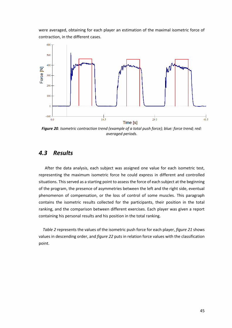
were averaged, obtaining for each player an estimation of the maximal isometric force of
contraction, in the different cases.
Figure 20. Isometric contraction trend (example of a total push force); blue: force trend; red:
averaged periods.
4.3 Results
After the data analysis, each subject was assigned one value for each isometric test,
representing the maximum isometric force he could express in different and controlled
situations. This served as a starting point to assess the force of each subject at the beginning
of the program, the presence of asymmetries between the left and the right side, eventual
phenomenon of compensation, or the loss of control of some muscles. This paragraph
contains the isometric results collected for the participants, their position in the total
ranking, and the comparison between different exercises. Each player was given a report
containing his personal results and his position in the total ranking.
Table 2 represents the values of the isometric push force for each player, figure 21 shows
values in descending order, and figure 22 puts in relation force values with the classification
point.

46
F PUSH FWD TOT F PUSH FWD LEFT F PUSH FWD RIGHT
INITIALS MEAN [N] ± SD MEAN [N] ± SD MEAN [N] ± SD Fright= tot(%)
Fleft
A.S. 268,95 ± 0,07 137,27 ± 4,75 199,20 ± 18,53 -45,12
B.A. 452,00 ± 8,02 239,07 ± 11,58 286,03 ± 16,88 -19,65
B.N. 324,30 ± 34,17 99,74 ± 2,01 130,80 ± 1,55 -31,15
B.M. 335,20 ± 14,25 155,23 ± 17,98 141,48 ± 39,96 8,86
C.A. 318,90 ± 25,76 156,97 ± 11,68 207,93 ± 29,21 -32,47
D.A. 198,10 ± 26,99 330,97 ± 8,97 283,47 ± 7,52 14,35
F.P. 250,00 ± 26,16 88,67 ± 1,79 104,67 ± 2,65 -18,05
F.A. 195,00 ± 11,37 150,07 ± 10,06 149,00 ± 13,31 0,71
F.S. 469,30 ± 19,68 347,03 ± 8,03 119,77 ± 5,46 65,49
G.D. 391,80 ± 20,79 284,80 ± 11,70 342,27 ± 18,11 -20,18
G.M. 271,10 ± 11,54 164,30 ± 4,17 222,27 ± 10,78 -35,28
K.H. 218,60 ± 17,26 165,90 ± 5,33 145,23 ± 8,59 12,46
M.P. 563,83 ± 35,32 514,93 ± 33,21 506,23 ± 18,74 1,69
Q.V. 384,03 ± 29,88 302,07 ± 17,45 166,30 ± 14,96 44,95
S.P. 148,30 ± 16,80 65,24 ± 2,52 71,23 ± 4,40 -9,18
T.G. 341,07 ± 35,20 159,17 ± 19,13 226,50 ± 41,11 -42,30
T.N. 417,83 ± 20,60 163,83 ± 20,26 228,33 ± 24,81 -39,37
V.L. 83,77 ± 16,50 235,53 ± 10,33 116,80 ± 1,90 50,41
Z.L. 457,47 ± 23,01 191,77 ± 14,64 171,27 ± 24,92 10,69
Table 2. Push forward force values [N]: mean and standard deviation. Difference between left and right side (%.)
Figure 21. Isometric push forward total force (both arms).
56
4
46
9
45
7
45
2
41
8
39
2
38
4
34
1
33
5
32
4
31
9
27
1
26
9
25
0
21
9
19
8
19
5
14
8
84
0
100
200
300
400
500
600
[N]
ISOMETRIC FTOT PUSH FORWARD

47
Figure 22. Isometric push forward total force in relation to the classification point.
The ranking of the maximum isometric force in the test of total pushing forward (figures
21, 22) generally agrees with the point of classification: points from 3.5 to 2.5 (with one
exception of V.L. due to a wrong measure) are in the first half of the ranking; points from
1.5 to 0.5 are in the second half. Therefore, people with more severe impairments develop
less force, because of the weakness of some muscles. In average, 3.5 points develop the
greater force; some of 2.5 points (Z.L., T.N.) exert the same force as 3.5 points (F.S., B.A.).
Some 1 and 1.5 points develop force values that are comparable to 2.5 points: this might
mean that 2.5, with some training, could increase their maximal force.
The following graphs (figures 23, 24) represent the ranking for the unilateral tests of
pushing forward.
Figure 23. Isometric push forward force with left and right arm (force values are sorted by the
left side).
M.P.
F.S.
Z.L.
B.A.
T.N.
G.D.Q.V
T.G.
B.M.
B.N.
C.A.
G.M.
A.S.
F.P.
K.H. D.A.
F.A.
S.P.
0
100
200
300
400
500
600
0 0,5 1 1,5 2 2,5 3 3,5
Iso
me
tric
Pu
sh F
WD
To
t Fo
rce
[N
]
Classification Point
51
5
34
7
33
1
30
2
28
5
23
9
23
6
19
2
16
6
16
4
16
4
15
9
15
7
15
5
15
0
13
7
10
0
89
65
50
6
12
0
28
3
16
6
34
2
28
6
11
7 17
1
14
5
22
2
22
8
22
7
20
8
14
1
14
9 19
9
13
1
10
5
71
0
100
200
300
400
500
600
[N]
ISOMETRIC FORCE PUSH FORWARD LEFT AND RIGHT
Left Right

48
Figure 24. Sum of isometric left and right push forward force in relation to total push forward
force.
Unilateral pushing forward tests give information about the difference between the left
and right side (table 2): values with the negative sign indicate that right force is higher than
the left force. For subjects where the difference among left and right side is high (apart from
the sign, more than 50%) it must be determined whether there is a diagnosed problem or
not, and eventually prepare a program of training for the weaker side.
Differently from bilateral tests, the unilateral push forward values do not follow the
ranking of classification (figure 23): this could be expected, because in pushing forward with
both arms, some mechanism of compensation can occur: on the contrary, the unilateral
exercises underline the personal impairments and can be read only in accord to the single
person’s disease.
Figure 24 represents the sum of left and right push forward values in relation to total
push forward values: the regression line reveals that the sum of left and right isometric push
force is in average 27% higher than the total push force (in this case, the wrong value of V.L.
was not considered to avoid altering the regression line).
The following tables (3,4) contain force values, with their standard deviation, for shoulder
and elbow flexion/extension.
M.P.
F.S.
D.A.
Q.V.
G.D.
B.A.Z.L.
K.H.;
G.M.
T.N.
T.G.
C.A.
B.M.
F.A.
B.N.
F.P.
S.P.
y = 0,7255x
0
100
200
300
400
500
600
700
800
0 100 200 300 400 500 600 700 800 900 1000 1100
Iso
me
tric
Pu
sh F
WD
To
t [N
]
Isometric Push FWD Left+Right [N]

49
SHOULDER FLEX LEFT SHOULDER EXT LEFT
SHOULDER FLEX RIGHT
SHOULDER EXT RIGHT
INITIALS MEAN [N] ± SD MEAN [N] ± SD MEAN [N] ± SD MEAN [N] ± SD
A.S. - ± - 155,60 ± 5,11 209,17 ± 5,69 179,57 ± 7,51
B.A. 317,77 ± 20,71 265,67 ± 9,76 237,80 ± 11,10 251,57 ± 6,30
B.N. 133,60 ± 1,56 34,26 ± 3,90 137,47 ± 11,34 49,69 ± 8,30
B.M. 76,33 ± 9,31 87,04 ± 1,18 62,68 ± 5,09 75,87 ± 2,66
C.A. 302,20 ± 4,33 151,63 ± 3,71 302,60 ± 4,42 67,97 ± 11,26
D.A. 152,13 ± 12,36 99,85 ± 10,19 209,57 ± 17,74 120,83 ± 0,76
F.P. 175,87 ± 5,64 79,00 ± 3,27 185,17 ± 11,10 62,66 ± 2,05
F.A. 146,87 ± 1,99 135,83 ± 6,80 112,33 ± 5,95 96,86 ± 9,84
F.S. 208,53 ± 6,00 150,87 ± 9,38 138,00 ± 3,27 66,65 ± 9,43
G.D. 132,00 ± 12,42 100,55 ± 3,98 120,40 ± 3,44 112,17 ± 5,26
G.M. 75,23 ± 16,22 88,58 ± 0,81 101,65 ± 4,81 57,80 ± 8,53
K.H. 109,70 ± 1,71 48,72 ± 4,12 91,66 ± 5,03 41,19 ± 1,25
M.P. 116,07 ± 11,18 120,83 ± 6,09 156,67 ± 9,90 125,50 ± 7,13
Q.V. 128,20 ± 13,48 124,17 ± 5,32 123,47 ± 5,35 113,00 ± 2,19
S.P. 33,20 ± 2,76 62,67 ± 0,93 96,45 ± 1,73 43,63 ± 8,25
T.G. 225,43 ± 10,97 95,32 ± 1,81 182,50 ± 41,40 82,06 ± 9,00
T.N. 129,33 ± 16,34 88,80 ± 7,98 111,93 ± 1,50 100,52 ± 15,13
V.L. 191,67 ± 19,52 108,78 ± 12,36 178,30 ± 10,50 91,90 ± 10,53
Z.L. 114,03 ± 16,24 91,79 ± 6,17 125,83 ± 18,07 95,96 ± 0,46
Table 3. Force values of shoulder flexion/extension left and right (A.S., F.P., F.A., S.P., T.G. performed the exercises with the wristband above the elbow).
ELBOW FLEX LEFT ELBOW EXT LEFT ELBOW FLEX RIGHT ELBOW EXT RIGHT
INITIALS MEAN [N] ± SD MEAN [N] ± SD MEAN [N] ± SD MEAN [N] ± SD
A.S. 211,97 ± 8,90 -51,46 ± 7,02 234,07 ± 32,60 -45,63 ± 1,58
B.A. 352,50 ± 77,17 -189,40 ± 16,81 186,60 ± 46,84 -118,73 ± 19,09
B.N. 243,00 ± 13,19 -193,63 ± 28,94 236,83 ± 60,23 -232,47 ± 10,87
B.M. 156,37 ± 17,41 -122,53 ± 17,70 226,37 ± 15,24 -105,37 ± 2,83
C.A. 87,84 ± 5,58 -127,07 ± 17,84 111,03 ± 11,91 -161,17 ± 5,90
D.A. 251,00 ± 5,75 -70,34 ± 5,41 281,87 ± 24,47 -204,87 ± 12,79
F.P. 184,87 ± 12,88 -18,71 ± 3,06 145,27 ± 18,32 -45,79 ± 4,16
F.A. 199,30 ± 57,03 -41,10 ± 6,60 187,57 ± 30,58 -75,71 ± 3,10
F.S. 260,43 ± 19,75 -176,30 ± 20,92 281,23 ± 17,89 -129,83 ± 14,23
G.D. 227,33 ± 6,00 -102,26 ± 3,61 260,63 ± 33,92 -217,00 ± 9,56
G.M. 171,00 ± 11,23 -115,73 ± 3,13 32,16 ± 7,17 -133,67 ± 3,28
K.H. 190,90 ± 13,05 -27,25 ± 1,01 89,08 ± 22,79 -22,93 ± 0,22
M.P. 290,25 ± 1,34 -287,85 ± 22,27 325,05 ± 7,57 -250,10 ± 7,07
Q.V. 220,40 ± 25,43 -183,23 ± 15,33 316,57 ± 12,99 -117,54 ± 17,85
S.P. 102,20 ± 7,22 -58,32 ± 2,87 159,10 ± 4,95 -14,81 ± 1,25
T.G. 199,97 ± 21,00 -55,30 ± 1,03 191,83 ± 13,04 -73,32 ± 7,52
T.N. 309,77 ± 10,23 -186,27 ± 11,10 309,33 ± 13,48 -134,00 ± 3,08
V.L. 301,07 ± 17,11 -169,33 ± 4,24 414,63 ± 7,91 -141,90 ± 27,21
Z.L. 238,87 ± 7,13 -213,97 ± 7,84 233,80 ± 27,35 -164,77 ± 2,73
Table 4. Force values of elbow flexion/extension left and right.

50
The following graphs (figures 25, 26) contain the ranking for the isometric force of
shoulder and elbow flexion/extension collected by the load cell, in descending order.
Figure 25. Shoulder flexion isometric force left and right (values are sorted by the left side).
Figure26. Shoulder extension isometric force left and right (values are sorted by the left side).
31
8
30
2
22
5
20
9
19
2
17
6
15
2
14
7
13
4
13
2
12
9
12
8
11
6
11
4
11
0
76
75
33
23
8
30
3
18
3
13
8
17
8
18
5 21
0
11
2 13
7
12
0
11
2
12
3 15
7
12
6
92
63
10
2
96
20
9
0
50
100
150
200
250
300
350
[N]
SHOULDER FLEXIONISOMETRIC FORCE - LEFT AND RIGHT
Left Right
26
6
15
6
15
2
15
1
13
6
12
4
12
1
10
9
10
1
10
0
95
92
89
89
87
79
63
49
34
25
2
18
0
68
67
97 1
13 12
6
92
11
2
12
1
82 9
6 10
1
58 7
6
63
44
41 50
0
50
100
150
200
250
300
[N]
SHOULDER EXTENSION ISOMETRIC FORCE - LEFT AND RIGHT
Left Right

51
Figure 27. Elbow flexion isometric force left and right (values are sorted by the left side).
Figure 28. Elbow extension isometric force left and right (values are sorted by the left side).
The results for isometric force rankings at elbow and shoulder do not follow the points
of classification. This was expected, since these values are strictly connected to each
personal disease. In some case, values highly differ between the left and right side.
Considering the shoulder flexion, for example, B.A., D.A. and G.M. have a high difference
between the left and the right side. This is due to the missing of the control of some muscles
of one side, in relation to the pathology. All these results must be correlated with medical
information, to find explanations for asymmetries or unexpected values.
35
3
31
0
30
1
29
0
26
0
25
1
24
3
23
9
22
7
22
0
21
2
20
0
19
9
19
1
18
5
17
1
15
6
10
2
88
18
7
30
9
41
5
32
5
28
1
28
2
23
7
23
4 26
1
31
7
23
4
19
2
18
8
89
14
5
32
22
6
15
9
11
1
0
50
100
150
200
250
300
350
400
450
[N]
ELBOW FLEXIONISOMETRIC FORCE - LEFT AND RIGHT
Left Right
28
8
21
4
19
4
18
9
18
6
18
3
17
6
16
9
12
7
12
3
11
6
10
2
70
58
55
51
41
27
19
25
0
16
5
23
2
11
9 13
4
11
8
13
0
14
2 16
1
10
5 13
4
21
7
20
5
15
73
46
76
23 4
6
0
50
100
150
200
250
300
350
[N]
ELBOW EXTENSIONISOMETRIC FORCE - LEFT AND RIGHT
Left Right

52
Finally, moments at the joints were
calculated with the multiplication of the force
collected by the load cell for the lever arm.
Considering the conditions of zero shoulder
flexion for shoulder exercise, the lever arm for
the shoulder moment is the total length of the
superior limb; considering the isometric
exercises at the elbow as executed with 90° of
elbow flexion, lever arm for the elbow
moment is represented by forearm length.
Arm and forearm lengths were measured for
each participant, and represented in table 5.
Arm length was taken from acromion to the
most proximal point on the lateral edge of the
radius, and forearm length from the latter
point to stylus.
INITIALS
SHOULD FLEX LEFT
MOM [Nm]
SHOULD FLEX
RIGHT MOM [Nm]
SHOULD EXT LEFT
MOM [Nm]
SHOULD EXT
RIGHT MOM [Nm]
ELB FLEX LEFT
MOM [Nm]
ELB FLEX
RIGHT MOM [Nm]
ELB EXT LEFT
MOM [Nm]
ELB EXT
RIGHT MOM [Nm]
A.S. - 125,50 80,91 93,37 55,11 60,86 -13,38 -13,69
B.A. 187,48 140,30 156,74 148,42 98,70 52,25 -53,03 -33,25
B.N. 76,15 82,48 19,53 28,32 60,75 59,21 -48,41 -65,09
B.M. 44,27 35,73 50,49 44,01 40,66 58,86 -31,86 -27,40
C.A. 157,14 169,46 78,85 35,34 19,32 24,43 -27,95 -40,29
D.A. 77,59 108,97 50,93 61,63 55,22 62,01 -15,48 -47,12
F.P. 102,00 105,55 45,82 36,34 48,07 37,77 -4,87 -11,91
F.A. 88,12 67,40 81,50 58,12 55,80 52,52 -11,51 -21,20
F.S. 125,12 82,80 90,52 39,99 72,92 78,75 -49,36 -36,35
G.D. 81,84 75,85 62,34 69,54 65,93 75,58 -29,66 -62,93
G.M. 39,12 56,93 46,06 30,05 37,62 7,08 -25,46 -33,42
K.H. 57,04 56,83 25,34 21,42 49,63 23,16 -7,09 -7,11
M.P. 71,96 100,27 74,92 77,81 81,27 91,01 -80,60 -72,53
Q.V. 71,79 79,02 69,53 63,28 61,71 88,64 -51,31 -37,61
S.P. 18,26 53,05 34,47 24,00 25,55 39,78 -14,58 -3,85
T.G. 130,75 105,85 55,29 47,59 53,99 51,80 -14,93 -19,80
T.N. 76,31 64,92 52,39 59,30 80,54 80,43 -48,43 -36,18
V.L. 118,83 108,76 67,44 56,98 87,31 120,24 -49,11 -39,73
Z.L. 67,28 74,24 54,15 56,61 64,49 63,13 -57,77 -46,13
Table 6. Moments at the joints in isometric elbow and shoulder flexion/extension.
ARM [cm] FOREARM [cm]
INITIALS RIGHT LEFT RIGHT LEFT
A.S. 300 260 300 260
B.A. 310 310 280 280
B.N. 320 320 280 250
B.M. 310 320 260 260
C.A. 310 300 250 220
D.A. 290 290 230 220
F.P. 310 320 260 260
F.A. 320 320 280 280
F.S. 320 320 280 280
G.D. 340 330 290 290
G.M. 310 300 250 220
K.H. 310 260 310 260
M.P. 350 340 290 280
Q.V. 320 280 320 280
S.P. 290 300 260 250
T.G. 310 310 270 270
T.N. 310 330 270 260
V.L. 330 330 280 290
Z.L. 310 320 280 270
Table 5. Anthropometric measures.

53
In some cases, moment values found for flexion/extension at the shoulder do not agree
with the results found in the literature (consider paragraph 3.4.3). This could be partially
imputable to an incorrect way of executing the exercise. Considering shoulder flexion, the
subject was asked to flex their arms seated on his sport chair, with a zero degree of shoulder
and trunk flexion: this situation did not always occur, since in some cases, to perform the
exercise, the subject flexed his trunk thus starting from a positive angle of shoulder flexion
(figure 29). Moreover, according to the execution protocol, the application of the wristband
to the wrist, to which the load cell was connected, allowed for an elbow flexion thus adding
an eventual moment generated by the biceps: this force was recorded by the load cell, but
was not imputable to the shoulder joint. In future measures, there is the need of applying
the wristband above the elbow, to make sure the recorded force in being the one exerted
by the shoulder flexion. Moreover, this would standardize the test according to those people
who do not have the control of his triceps and necessary need a fixation above the elbow,
to execute a movement of isometric shoulder flexion/extension.
Also the moments of elbow flexion/extension do not always agree with literature results.
This is probably still due, partially, to a wrong phenomenon of compensation occurring
during the movement of some subjects. Moreover, the force was exerted through a
carabiner attached on the external part of a plastic disk: in this way, the force was not
parallel to the load cell direction, and the beam flexed. Some people performed the
exercises with an elbow extension different from 90° (figure 30). In elbow flexion, some
subjects helped the movement with a shoulder extension and elevation; in elbow extension,
some people helped the movement with a shoulder adduction. This could add some
advantage on the force, especially in those cases in which muscular control is weak, and is
recorded by the load cell.
Figure 29. Shoulder flexion test. Left: wrong way of execution (positive angles of elbow and trunk flexion). Right: right way of execution (zero elbow and trunk flexion).

54
Figure 30. Elbow extension test. Left: wrong way of execution (shoulder abduction, less than 90° of elbow flexion, the applied force is not parallel to the beam). Right: right way of execution
(no trunk rotation, 90° of elbow flexion, force parallel to the beam).
For these reasons, the whole set of isometric measure must be repeated assuring the
movement to be pure as much as possible, avoiding effects of compensation and extra
forces not related to the specific joint moment.
The result reported in literature [19,23] also differ for the fact that in cited studies,
isometric tests were executed in healthy and non-trained people: the present study, on the
contrary, is based on wheelchair-users athlete, so their level of training of the upper limbs
in some cases (as B.A., T.G., M.P., F.S.) is very high.

55
CHAPTER 5
Project activity 2: dynamic tests
Wheelchair Rugby is a very tactic game, based not only on mere athletes’ muscular force,
but much more on the way the athlete can use his force to express particular abilities and
skills within the game. Impressing a good acceleration, velocity, and spinning, combined
with a team play, are some of the most important features that a Wheelchair Rugby athlete
has to learn and improve. Therefore, some situations present the necessity of impressing a
big acceleration from a still position, for example to reach to the goal line or to receive the
ball from a mate; another necessity is the ability of turning quickly, in situations as blocking
an opponent or freeing from a blockage position.
This sport was born to give people with an incomplete upper limbs and trunk muscular
control, the chance to compete using their residual capacities at best: in this way, athletes
with low points and most severe impairments can have an essential role within the game.
In this work, the dynamic performances of athletes were investigated by measuring their
longitudinal acceleration and angular velocities in different situations, through MEMS
inertial sensors.
Research question: considering the wheelchair-user system, what are the maximum and
mean forward acceleration in a sprint, eight track and during a match? What is the maximum
angular velocity in a rotation and in an eight track?
5.1 Instrumentation
This paragraph describes the meaning of MEMS sensors (accelerometers and
gyroscopes), and Xsens inertial sensors used in this work for the data acquisition, with the
protocol for their fixation in wheelchairs to perform dynamic tests.
5.1.1 MEMS inertial sensors
Micro Electronic Mechanical Systems, or MEMS, is a technology obtained using the
techniques of microfabrication. The physical dimensions of MEMS devices range from below
one micron to several millimetres. The types of MEMS devices vary from simple structures
having no moving elements, to extremely complex electromechanical systems with multiple
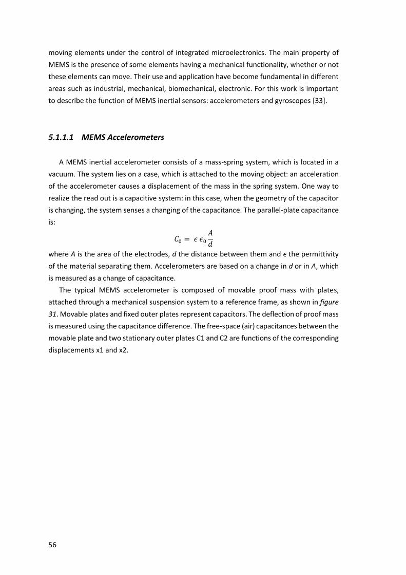
56
moving elements under the control of integrated microelectronics. The main property of
MEMS is the presence of some elements having a mechanical functionality, whether or not
these elements can move. Their use and application have become fundamental in different
areas such as industrial, mechanical, biomechanical, electronic. For this work is important
to describe the function of MEMS inertial sensors: accelerometers and gyroscopes [33].
5.1.1.1 MEMS Accelerometers
A MEMS inertial accelerometer consists of a mass-spring system, which is located in a
vacuum. The system lies on a case, which is attached to the moving object: an acceleration
of the accelerometer causes a displacement of the mass in the spring system. One way to
realize the read out is a capacitive system: in this case, when the geometry of the capacitor
is changing, the system senses a changing of the capacitance. The parallel-plate capacitance
is:
𝐶0 = 𝜖 𝜖0
𝐴
𝑑
where A is the area of the electrodes, d the distance between them and ϵ the permittivity
of the material separating them. Accelerometers are based on a change in d or in A, which
is measured as a change of capacitance.
The typical MEMS accelerometer is composed of movable proof mass with plates,
attached through a mechanical suspension system to a reference frame, as shown in figure
31. Movable plates and fixed outer plates represent capacitors. The deflection of proof mass
is measured using the capacitance difference. The free-space (air) capacitances between the
movable plate and two stationary outer plates C1 and C2 are functions of the corresponding
displacements x1 and x2.

57
Figure 31. Typical MEMS accelerometer structure. The proof mass is attached through springs (kS is the spring constant) at the base substrate. It can move only up and down. Movable and
fixed plates form capacitors.
This was an example of one axis accelerometer. If one circuit includes sets of capacitors
in perpendicular directions, it is possible to obtain a two or three axis accelerometer, as
shown in figure 32 [34].
Figure 32. Left: 3D accelerometer structure. It has three different sensors for x-y-z axis acceleration and three different electronic circuitry for each axis. Right: An ADXL 320
accelerometer.

58
5.1.1.2 MEMS Gyroscopes
A MEMS gyroscope uses the Coriolis effect to measure an angular velocity. This effect
states that an object with mass 𝑚 and velocity 𝒗(𝑡) in a rotating plane with angular velocity
𝜔(𝑡), receives an apparent force 𝑭𝑪𝒐(𝑡) , the Corilois force, proportional to 𝜔(𝑡) and 𝒗(𝑡):
𝒂𝑪𝒐(𝑡) = 2𝜔(𝑡) × 𝒗(𝑡) 𝑭𝑪𝒐(𝑡) = −𝑚 𝒂𝑪𝒐(𝑡)
Measuring the effects of this force on the oscillating object, the characteristics of the
movement can be obtained. According to this physical law, a MEMS gyroscope can be
realized in many ways (an example on figure 33): vibrating ring, macro laser ring,
piezoelectric plate ring, fiber optic and tuning fork gyroscope, which is one of the most
widely used gyroscope. Tuning fork gyroscope is composed by two proof masses that are
built in such a way as to oscillate with the same intensity but in opposite directions. When
rotated, a Coriolis force is generated, that it is bigger when mass is further away from the
spin: this creates an orthogonal vibration that can be detected by different methods.
Figure 33. Left: SEM tilt view of a MEMS gyroscope; right: L3G4IS, the first three-axis MEMS gyroscope.
The Xsens inertial sensor used in this work, has a MEMS rate gyroscope, with a beam
structure and capacitive readout.
5.1.2 Xsens technology The Xsens wireless Motion Tracker (MTw™) is a miniature wireless inertial measurement
unit (IMU) realized with MEMS technology. It contains 3D accelerometers, 3D rate
gyroscopes, 3D magnetometers and a barometer (pressure sensor). The embedded
processor handles sampling, buffering, calibration and Strap Down Integration (SDI) of the
inertial data, as well as the wireless network protocol for data transmission. SDI is a method
to compute an orientation or position changing given an angular velocity or acceleration of

59
a rigid body. The Xsens provides real time 3D orientation for wireless motion trackers in a
network, returns 3D linear acceleration, angular velocity and (earth) magnetic field and
atmospheric pressure data. The system used in this work consists in:
Motion Tracker wireless sensors (MTw’s™):
portable sensors with their own battery (figure
34). All wireless motion trackers send data
wirelessly to the PC, via the Awinda Station™,
placed on the desk next to the recording PC.
Awinda Station™ that controls the reception of
synchronised wireless data from all wirelessly
connected MTw™ sensors, and charges up to 6 of
them simultaneously (figure 35); it is connected
via USB with the PC for data acquisition;
MT Manager™ Software for visualising and recording data; it is possible to see the
real time orientation of the connected sensor, together with their angles values,
acceleration trend, magnetic field.
Sensors specifications are represented in the following table:
Table 7. Main sensing specifications.
The patent-pending Awinda™ radio protocol is based on the IEEE 802.15.4 PHY. Using
this basis, ensures that standard 2.4 GHz ISM chipsets can be used. The Awinda protocol
Figure 34. MTw™ inertial sensor.
Figure 35. Awinda Station™.
60
provides time synchronisation of up to 32 MTw’s across the wireless network to within 10
μs. With Awinda, the data are initially sampled at 1800Hz, down-sampled on the processor
of the MTw to 600Hz, and using Strap Down Integration (SDI) the data are transmitted to
the Awinda Station. Output sample rate of the MTw’s™ can be chosen by the user and
changes with the number of connected sensors: with one MTw™ connected, the maximum
frequency is 120 Hz; with two, the higher frequency automatically decreases to 100 Hz, and
so on. The lower frequency is 20 Hz. Each MTw™ is powered with its own LiPo battery. At its
current state of use, the battery lasts for almost 2 hours and can be recharged after one
hour docked in the Awinda Station™ [35].
5.1.2.1 Xsens system of orientation
Each MTw™ has a right handed fixed coordinate system, that defines the sensor
coordinate frame S (figure tot). This frame is aligned with the sensor's external box but the
real reference is inside and, of course, this may cause an error and a loss of accuracy. The
internal angles are defined as Euler "aerospace" angles, called in this way because they are
frequently used in aerospace field, defined the RPY convention, where R is "Roll", P is "Pitch"
and Y is "Yaw". Following to the right hand rule, the Roll angle is around X axis, Pitch is
around Y, Yaw is around Z.
The alignment between the coordinate system S and the bottom of the MTw™’s box is
guaranteed less within than 3°. Another problem of the inertial sensors in the orthogonality
of the reference system’s axes, but regarding Xsens MTw™ the non-orthogonality is less
than 0.1°. In default conditions each MTw™ returns angles between the coordinate system
S and the “Earth” coordinate system E, with E as reference coordinate system. E coordinate
frame is called “Earth” because it is “created” by Earth with its magnetic field and its gravity
acceleration axis, it is defined as a right handed coordinate system as follows:
X axis has the same direction and orientation of a vector that points to the Earth
magnetic North;
Y axis is calculated according to the right hand rule;
Z axis has the same direction of gravity force but opposite orientation.
The E coordinate system is invariable, therefore to perform a clearly and more intuitive
description of the reset operations, it has been created a new coordinate system called Fixed
coordinate system F. Hence F is taken as the reference coordinate system and in default
conditions coincides with E (figure 36).

61
The software offers several options of reset, that differ for the output angles of the S
coordinate frame. The most complete option is the alignment reset (figure 37): with this
operation, the MTw’s™ output angles of Roll, Pitch and Yaw are put at zero degrees. As
shown in figure 37, a new internal frame S’ is aligned with the new F’ fixed coordinate
system. In this work, this option was chose to perform the measures.
Figure 37. Alignment reset of an MTws™.
Figure 36. MTw’s coordinate system

62
5.1.3 Sensor fixation
To perform dynamic measures, Xsens MTws™ were put in the same positions for each
wheelchair: one on the frame, and one for each main wheel, as described in the following
paragraphs.
5.1.3.1 Wheelchair frame sensor
The wheelchair frame sensor allows recording the forward acceleration and angular
velocity of the system in movement. Considering the wheelchair-player system, its
reference frame is considered with the origin in its Centre of Mass (COM), the X axis in the
direction of movement (horizontal), the Z axis in the vertical plane and the Y axis obtained
with the right hand rule. To measure the forward acceleration of the system and its angular
velocity, the sensor must be ideally placed in the COM, but since its spatial coordinates are
unknown, this is not possible: therefore, its position in the wheelchair frame is given by the
centre of the beam connecting the wheels’ axles. The Xsens is placed in a horizontal plane,
with the X axis parallel to the wheelchair-user’s X axis, as represented in figure 38.
Figure 38. Player in its reference frame (black); Xsens reference frame with Roll, Pitch and Yaw
angles.
A support was attached to the wheelchair frame to fix the sensor. Since each frame had
a slightly different structure, the support and its fixation were adaptable. We used the bends
given from the Xsens set, which are provided with a click-mechanism that allows the sensor
to be easily fixed. The protocol for the fixation is described in the following points:

63
1. Sensor connection to the Awinda Station. After choosing a full-battery Xsens, it was
connected to the radio station.
2. Sensor reset: the sensor used for the test was placed on the floor (after verifying it to
be horizontal with a level), with the X axis parallel to a straight line (e.g. following a line
of the court). Using the option of the alignment reset, we assured that the internal
system of orientation of the sensor was concordant with the global system of reference.
Moreover, it was important to assure that there was no flipping phenomenon: the
software can register an axis rotation even if the sensor is not moving. In this case is
better leaving that sensor resting for some minute, waiting this phenomenon to be over.
3. Support and sensor placement. There were some needs to correctly position an Xsens
with its support in the wheelchair frame:
o the sensor has to be placed in the longitudinal-middle plane of the wheelchair
frame (ideally in the point of intersection of the wheels’ axles). The support was
fixed in the beam just under the seat, which connects the wheels’ axles.
o Xsens’ X axis has to be aligned in the longitudinal direction of the wheelchair: in
this way the acceleration recorded in that direction is the forward acceleration.
To do this, the wheelchair was placed following a court line as its longitudinal
line (figure 39). In this way we knew that when the Yaw angle is zero, the X axis
of the sensor is aligned in the longitudinal direction.
Figure 39. The red line is a hypothetical court line; the Xsens’ X axis is aligned with the red line.
We used the sensor’s system of reference to correctly align it: with the sensor on
the support, not yet fixed, we identify its correct position when Roll and Pitch angles
are zero (with a tolerance error of ±4°), we first fixed the support and then attach
the Xsens on it. Even if there was the aim of placing the sensor minimizing the

64
horizontal (Pitch) angle, an error of some degrees was always committed. But, as
verified in signal analysis, this did not affect the measures.
Figure 40. Wheelchair with sensors (frame and wheels).
5.1.3.2 Wheel sensors
An Xsens was placed on each wheel, to evaluate the velocity of rotation and the number
of turns. After removing the wheels, a plastic support was fixed in the axle, and on it, an
Xsense with the X axis in the direction of the axis of rotation of the wheel, oriented
externally, to record wheel angular velocity (Ang vel Xw). The setting is shown in figure 41.
Figure 41. Sensors in the wheels. Left: wheel system of reference; right: sensors fixation.

65
5.3 Methods
In this work, the Xsens was used to measure the longitudinal acceleration and the angular
velocity of wheelchair rugby players in different kinds of exercise, to obtain a quantitative
evaluation of their performance on court.
5.3.1 Tests description
From the literature and the observation of the match, it was decided to evaluate the
ability to push and finally brake during a 20 m linear sprint, the ability of turning left and
right on spot, an 8 track which is more similar to a real game, combining linear sprint with
turning. Finally, a match was analised.
5.3.1.1 20 m sprint
The 20 m sprint is a time exercise assessing the ability of the player to push with his arms,
as much and fast as possible. It corresponds to an explosive performance. In this path, the
subject was asked to reach his maximum acceleration in 20 m and, once having passed the
final point, brake instantaneously. In this way it was possible to measure the trend of the
forward acceleration during the push phase, and the negative acceleration given by braking.
Players started from a fixed position (figure 42), without moving, with the front castors
aligned in a given line.
Figure 42. An athlete at the starting position for 2the 20m sprint (yellow arrow).

66
The Xsens started its acquisition when the subject was well positioned in the start line: in
this way, the initial time of the longitudinal acceleration was visible on the recorded signal
as an initial high positive value after a time of zero acceleration.
At the signal of “go” the player started pushing: time was counted with a hand
chronometer. Once he passed the final cones, time was stopped and the Xsens acquisition
was stopped few seconds after the final braking. This exercise was repeated three times,
with a brief recovery (almost one minute) after each trial.
5.3.1.2 Rotation
In this exercise, the subject was asked to rotate on place (figure 43) to evaluate his ability
to turn left and right and the eventual difference on the performance between the left and
the right side, measuring the Z angular velocity of the frame sensor.
Figure 43. Left rotation; right rotation.
The player started from a given position, and at the signal of start, he executed as fast as he
could, a 360° turn on place, in the right direction, trying to turn around the vertical axis that
ideally passes through the point of intersection of the wheel axis (the Z axis of wheelchair-
player reference frame). Three seconds after the first rotation, he turned on the other
direction. This left-and-right session was repeated three times, with a brief recovery (10 s)
between each trial. Xsens registered each trial.
5.3.1.3 Eight track
The eight track is a time exercise, described by cones, in which linear acceleration and
rotation are combined: this is more similar to a real game situation. During this exercise we
measured the linear acceleration and the Z angular velocity of the player.

67
The path is shown on figure 44.
Figure 44. The red points represents the cones. First: distances between cones;
second: 8 track (blue lines) from start to final point.
The subject started from a given position (figure 45) and after the signal of “go”, he started
pushing. Time was stopped when he passed the last two cones. This exercise was
repeated three times, with a brief recovery (almost one minute) between each trial.
Figure 45. Eight track from starting position.
5.3.1.4 Match
The most important moment for an athlete is the match: in this contest, he has the
chance to express at best all his abilities, with the additional help given by the motivation,

68
which has a very high impact on the physical performance. Moreover during a match, the
game situations are different and complex: sprints, impacts, falls, backward pushes and
many others. On the other hand, dynamic tests give information about abilities as
accelerating, braking and spinning, in particular controlled conditions, but this parameters
acquire another relevance when collected on court, which is the real situation in which the
athlete acts. For this reason, in this work, acceleration and angular velocity during a match
were recorded and analysed.
To perform these measures, an Xsens was fixed on the wheelchair frame (as described
in the previous paragraph) of the 8 athletes on court. The entire match were recorded. A
GoPro or a digital camera, to visually synchronise the inertial signals with the event, also
recorded the match.
5.3.1.5 Friction
The frame Xsens was used to record some friction tests: the subject was asked to start
from a still position and then push for 6 m and let him go without pushing further. The aim
was to determine the deceleration which was totally imputable to the numerous factors
which creates friction. Nevertheless, it was impossible for the subject to go straight because
of the shape of the wheels, which are generally bent for overuse. Therefore, the necessity
to correct the direction touching the wheel distorted the measure. This test will be executed
in different conditions.
5.3.2 Signal analysis
The MT manager software saves the Xsens file as MT binary log file (.mtb). The aim of
the signal analysis is the extraction of:
max and mean values of forward acceleration for the 20 m sprint;
maximum value of left and right angular velocity in rotation tests;
maximum value of forward acceleration and of left and right angular velocity in eight
track tests;
maximum forward acceleration and distribution of acceleration values within a
match.
Before dealing with the elaboration, it is important to interpret the recorded signals and
associate their characteristics to physical phenomenon occurring during the test.

69
5.3.2.1 Frame sensor
Considering, as an example, a 20 m sprint test, the MT Manager™ output about inertial
data coming from the frame sensor are represented in figure 46. The MT Manager™
software gives data about acceleration, angular velocity and magnetic field on the three axis
of the sensor; in the present work the magnetic field was not studied.
Figure 46. Frame sensor, inertial data of a 20 m sprint (V.L.): acceleration, angular velocity and
magnetic field. X is the forward direction of movement.
According to the sensor’s fixation, longitudinal acceleration of the wheelchair-player
system is Acc X (with the sign concordant to the direction of movement) while Acc Y refers
to the transversal direction (directed on the left). The forward acceleration trend, in the
propulsion phase, can be considered as periodic: it is possible to notice positive and negative
peaks corresponding to the pushes, as described in literature. Pushes visually occur with a
given frequency that characterizes the personal subject’s propulsion technique.
Oscillations occur also along the transversal direction: Acc Y shows an oscillating trend,
with a smaller range of values than forward acceleration, and with no periodicity. This
component is associated to lateral movements and is always recorded in wheelchair

70
propulsion. Depending on the player’s pushing style, transversal acceleration values vary;
nevertheless, in the linear sprint recorded in this work, the maximum Acc Y positive peak is
always less than 50% of the maximum Acc X value.
Xsens is also sensitive to the gravitational acceleration: even if the sensor is not moving,
Acc Z starts from a positive value (almost 10 m/s2). Mtw’s™ system of reference, after the
alignment reset, is oriented with the Z axis parallel to the vector of the gravity force, but
with opposite sign. After the fixation, the sensor is nearly parallel to the ground: therefore,
the gravitational force is only recorded along the sensor’s Z axis.
Acc Z trend presents oscillations during the propulsion phase: this is due to player’s
movements around Y axis. Therefore, during the propulsion, the wheelchair-player system
always changes its points of contact with the ground: it shifts from an anterior support on
the front casters and posterior support on the main wheels, to an anterior support on the
main wheels and posterior support on anti-tip devices. Considering the normal
configuration of the wheelchair, that is the anterior support on front casters, anti-tip devices
are, for their own function, lifted from the ground (of max 2 cm): for this reason, a posterior
support on them, makes the whole system tilt slightly backward. This continuous shifting,
caused by the trunk and arm movement of the user, is recorded by the sensor and can be
seen in Acc Z trend.
Another evidence of this fact is the angular velocity around the Y axis (Ang vel Y): it is
possible to notice that the trend is characterized by a sequence of positive and negative
peaks, at the same frequency of the pushes (as visible in figure 46, the number of positive
peaks is the same).
Ang vel Z represents the angular velocity around the vertical axis of the wheelchair,
concordant (with some degree of error due to the fixation) to the Yaw axis of the sensor.
The positive verse corresponds to a left rotation, the negative to a right rotation. From the
Z angular velocity trend, is possible to determine a characteristic of the pushing style of the
player. Therefore, some players used to propel with an alternate push, especially when
starting from a still position: indeed, for some people, it is easier not to use both arms
contemporary, but to exert a push with one arm and then a push with the other arm. This
is evident in the Z angular velocity, as this style causes higher degrees of rotation of the
whole system, if compare with a normal push (figure 47).

71
Figure 47. Acceleration and angular velocity trends of a 20 m sprint (N.B.), for an alternate
pushing style, visible in the first three pushes. Forward direction is Y, transversal direction is X.
In this case, for a particular configuration of the wheelchair frame, the sensor was fixed with
a right 90° rotation around the Z axis to allow its fixation: the forward direction is Y and the
transversal direction is X. The first three pushes are alternate (Ang vel Z), and generate high
values of angular velocity around Z (to 90 deg/s), while a normal style generates lower
values (50 deg/s). In the first three pushes, the transversal acceleration component has
higher values than in the rest of the signal, comparable to the forward acceleration values;
the forward acceleration is lower in the first three pushes, to consequently increase and
assume a repeatable shape.
The MT Manager™ Software also records the space orientation of the MTw’s™,
represented in figure 48.
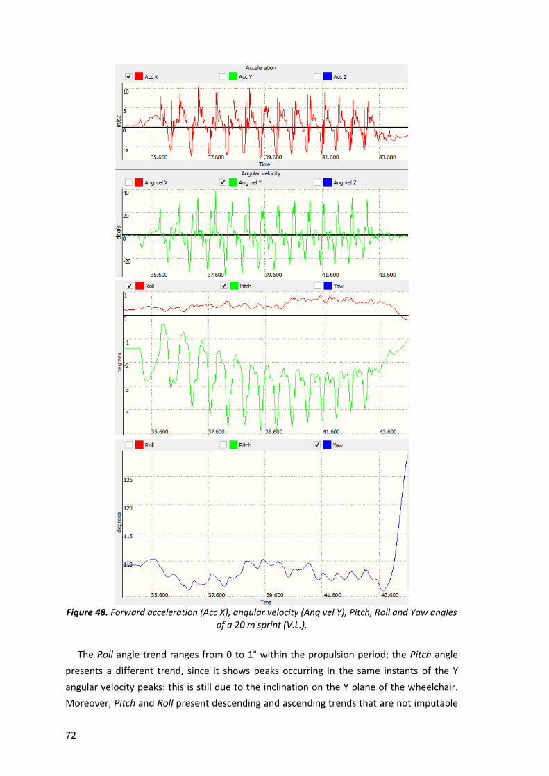
72
Figure 48. Forward acceleration (Acc X), angular velocity (Ang vel Y), Pitch, Roll and Yaw angles
of a 20 m sprint (V.L.).
The Roll angle trend ranges from 0 to 1° within the propulsion period; the Pitch angle
presents a different trend, since it shows peaks occurring in the same instants of the Y
angular velocity peaks: this is still due to the inclination on the Y plane of the wheelchair.
Moreover, Pitch and Roll present descending and ascending trends that are not imputable

73
to any physical phenomenon, but seem to be random. The Yaw angle registers the rotation
around the Z axis. The angles trend can be easily seen in Matlab, as shown in figure 49.
Figure 49. Forward acceleration (Acc X), angular velocity and angles of a 20 sprint (L.V.).
The graphs represent the whole period before the subject executed the test, starting from
a still position. It is possible to verify that the Pitch angle varies even if the person is not
moving in that direction: this seems to be related of some phenomenon internal to MTw’s™
gyroscope. Nevertheless, this range of variation of some degree, does not affect the
measure, the sensor can be approximated as placed in a horizontal plane, and the X
acceleration can be considered as the forward acceleration. In fact, considering Roll angle
as zero, a Pitch inclination error of some degrees does not substantially vary the forward
acceleration value. In composing the acceleration, the cosine component should be
evaluated:
𝐴𝑐𝑐ℎ𝑜𝑟𝑖𝑧𝑜𝑛𝑡𝑎𝑙(𝑡) = 𝐴𝑐𝑐𝑋(𝑡) ∙ cos (𝑃𝑖𝑡𝑐ℎ(𝑡))
In this case, if the Pitch maximum value is 4°, cos(4°)=0.9976. The acceleration values vary
of a maximum 0.2%. In other situations, Pitch value till 10° occurred, bringing an
acceleration error of 1.5% that is still acceptable.
Before describing the data analysis, the following paragraph contains some
considerations about the wheel sensors.

74
5.3.2.2 Wheel sensors
The Xsens inertial data coming from the left and right wheel sensor are represented in
figures 50, 51. The difference of fixation determines the difference of sign, but the values in
their module are comparable.
Figure 50. Right wheel sensor, inertial data of a 20 m sprint (V.L.): acceleration, angular
velocity and magnetic field.

75
Figure 51. Left wheel sensor, inertial data of a 20 m sprint (V.L.): acceleration, angular velocity
and magnetic field.
Acceleration values do not start from zero, even when
the sensor is not moving: this is due to the
gravitational acceleration, that is recorded by the
Xsens. Differently from the frame sensor, a wheel
sensor generally presents considerable values of Roll,
Pitch and Yaw before the starting moment (figure 52):
for this reason, even when the sensor is not moving, a
component of the gravitational acceleration is felt
along all the sensor’s axis and recorded as a non zero
value.
Because of the fixation on the wheel, the sensor’s X axis was parallel to the wheel axis,
with an error due to the axles’ thickness (nearly 2 cm): for this reason, considering the
acceleration trends after the start, Acc X shows small values if compared with the other two
Figure 52. Spatial orientation of the left wheel sensor in the fixed
position before the start.

76
components of acceleration. Acc Y and Acc Z present a periodicity at the same frequency,
but not in phase because of the rotation of the wheel.
The angular velocity trend is relevant only for the X component: considering the left
sensor, it is possible to notice a crescent trend (for the right wheel sensor, this trend is
negative) with some oscillation, in phase with the forward acceleration trend of the frame
sensor. Visually, the number of pushes is the same and correspond to the variation of
velocity of the wheel caused by the push. The crescent trend underlines the fact that the
velocity does not remain constant but increases during the whole sprint, more quickly in the
first phase and less in the last phase of the sprint. Probably, if the test had been executed in
a longer distance, the velocity trend had stabilized at a net constant value, without
increasing further.
5.3.2.3 Pre-elaboration
Signals coming from the frame Xsens are then exported as text files and then imported
in Matlab MathWorks R2015a. The imported data are acceleration (Acc_X, Acc_Y, Acc_Z)
and angular velocity (Gyr_X, Gyr_Y, Gyr_Z).
Each signal was pre-elaborated to compensate some errors coming from the acquisition.
A common error is the drift. The signal always presents an offset error: it registers a non-
zero value (positive or negative), even if the sensor is not moving: this value is called drift
(figure 53). This situation is always occurring: when the error is more than 5% of the signal’s
SD, the value was algebraically subtracted from the whole signal.
Figure 53. Red: Forward acceleration trend during a 20 m sprint (Z.L.); blue: drift value.

77
The drift is always easy to identify since during each dynamic test, Xsens acquisition
started when the athlete is in a still position: in this way the signal always starts from the
zero (drift) value. To evaluate the drift, it was identified an initial interval of samples in which
the signal remains stable, and made an average of those values. In most cases, drift was
irrelevant but sometimes, it reaches considerable values (even more than SD, as in figure
53). This phenomenon seems to be random: it can happen in two consequent acquisitions
of the same sensor, with different values.
5.3.2.4 Data analysis of 20 m sprint
The signal that describes the test of 20 m sprint is the longitudinal acceleration of the
wheelchair-player system. It has the property of being periodic during the propulsion phase
of the test, for this reason it was analysed using the frequency domain and the Power
Spectral Density (Appendix 1).
For each Xsens file coming from the acquisition of a 20 m sprint, the signal of the
longitudinal acceleration was imported in Matlab. The typical graph is shown in figure 54. It
is possible to notice the propulsion phase characterized by a number of pushes with a
maximum peak for each one, and the final braking with a higher negative value of
acceleration. The shape of each push is comparable with the other, and during the test, the
movement of the athlete itself takes place in a continuous cycle of pushing and recovering:
for this reason the signal presents a periodicity.
Figure 54. Trend of the longitudinal acceleration during a 20m sprint (K.H.).

78
The parameters chosen to represent this performance are the maximum value of
acceleration of the entire signal, mean of the peaks of pushes, and the minimum peak of
negative acceleration (deceleration), during braking.
After a pre-elaboration of the signal, to extract these values, the Matab protocol for 20
m acceleration analysis is described in the following lines (in Appendix 2, the full code).
1. Graphical identification of the propulsion interval of time. The part of the signal
undergoing the analysis is graphically identified from the end of the first push, to the
last push (before the braking), as shown in figure 55.
Figure 55. Red line: longitudinal acceleration, from the second to the last push
(considering the trend represented in figure 54). Blue markers: maximum peak of each push.
The first push is always different from the others, for shape and duration: it is slower
and with a lower peak, so it is not comprised in the Fourier analysis.
2. Fourier transform of the signal. The DFT via the fft Matlab function is calculated from
the selected part of the signal.
3. Power Spectral Density. The PSD is calculated with the expression in Appendix 1.
4. Definition of the frequency domain. The frequency domain is from zero to the
sampling frequency.
5. Selection and visualization of the first half of PSD samples. The spectrum is plotted
in the frequency domain.
6. Identification of the pushes frequency (PF). In the examined cases, PF was always
comprised between 1-3 Hz. Any eventual peak in the spectrum corresponding to
lower frequencies was not taken into account.

79
7. Division of signal into pushes.
8. Peak detection. For each push, the higher value is evaluated as a peak (figure 55).
9. Mean of peaks. Mean acceleration is calculated as an average operation between
the peaks higher than a chosen threshold (50% of max value of acceleration). After
the visualization, it is possible to eliminate any eventual wrong peak.
10. Braking identification. The negative value of braking is identified graphically as the
lower value of the negative trend, after the last push.
The values of maximum, mean acceleration and braking of each of the three trials were
then averaged.
5.3.2.5 Data analysis of Rotation
The signal considered to evaluate the ability of rotating on place is the angular velocity
around the Z axis of the frame sensor (Ang vel Z). The MT Manager™ software automatically
exports values in rad/s so the first operation is their conversion in deg/s: figure 56
represents the typical trend.
Figure 56. Z angular velocity trend in a rotation test (K.H.).
The positive values correspond to the left rotation: according to the orientation of the Xsens
in the wheelchair frame, and to the right-hand rule, left angular velocity has the positive
sign. The negative values represent right angular velocity. In those cases in which the sensor

80
fixation was different, its orientation has to be taken into account to correctly identify the
right and left peak values.
For each trial, the maximum and the minimum value (in module) of the angular velocity
were identified with the proper Matlab function. The values extracted from each trial were
averaged, giving a maximum left and right angular velocity value for each player.
5.3.2.6 Data analysis of 8 Track
Eight track performance parameters are determined as maximum acceleration and
maximum left and right angular velocity values during a trial. Angular velocity was converted
in deg/s, and its values were extracted as for the rotation test. The typical trend is
represented in figure 57.
Figure 57. Eight track acceleration and angular velocity (K.H.).
The first set of pushes is visible in the acceleration trend, then in the velocity trend there is
the right rotation around the second cone and the left rotation around the first cone, and
finally the last set of pushes with lower values due to the deceleration. The temporal
location of the maximum value of acceleration differs among the players: it could be
reached during the first pushes before turning around the first cone, after the rotation
around the last cone, or as shown in figure 57, between the two middle cones rotation. It
was never recorded a situation in which the maximum acceleration value corresponds to
significant values of rotation.
The values extracted from each of the three trials were then averaged, and the standard
deviation of the measures was evaluated. The result was a unique value of max acceleration

81
and max left and right angular velocity, which characterize that type of performance, for
each player.
From the wheel sensors data, recorded during the eight track, the angular velocity
around the wheel axis was extracted (Ang vel Xw). To calculate the distance covered by the
wheels in the track, the velocity signal was integrated, obtaining the number of degrees of
each wheel during the test, and consequently the total number of turnings. The
multiplication for the circumference of the wheel gives the total path (in metres) made by
each wheel. For the analysed cases, this distance of both wheels is near 22 m, since the path
was symmetrical.
Figure 58 shows the frame signals of forward acceleration and angular velocity, and the
correspondent wheel sensors signals of angular velocity, with the trend of the space made
by the wheels, in metres. The sing of right angular velocity was turned into positive, to allow
representing for both wheels a positive angular velocity while the system is going forward.
It is possible to notice that after the first set of pushes, in which wheels angular velocity
increases with a comparable trend, the left trend of angular velocity quickly decreases,
reaching small values: in that moment the system is starting turning left (around the first
cone) so the left wheel is braking (maintaining the same rotation direction). The same
situation occurs for the right wheel, before the right rotation around the second cone.
At the end of the track, wheels covered distance is comparable since the 8 track path is
symmetrical: in this case, any difference in wheels covered distance can be imputable to
phenomenon of slipping.

82
Figure 58. Eight track signals from frame and wheels sensors (Q.V.).

83
Data analysis of wheel sensors in eight track was made for a future development, to
determine the distance covered by the wheelchair-player system in a match: since COM
position is unknown, it was approximated as placed in the middle point (MP) of the beam
connecting wheel axles, that is the point of fixation of the frame sensor.
Considering forward acceleration of an eight track, after a first integration to obtain
velocity and a second integration to determine the space, the final result is a difference (till
30%) between the distance obtained by integration of wheels angular velocity, and that
obtained by the frame sensor. This occurred because the space covered by the MP can be
obtained from forward acceleration only if the person is going straight, without rotating:
therefore, in the same analysis made for the 20 m sprint, distance from wheels and from
MP coincide, since the movement takes place in an unique direction. Eight track is a different
situation: considering the MP, there are parts of the forward acceleration signal in which
the trend is very close to zero, in relation to the fact that the player is, for example, turning
around the cone and consequently not impressing a positive acceleration. An integration on
that signal, to obtain space, would bring to wrong results.
Considering the signal of angular wheel velocity, three situations can occur:
o player is going straight: wheels are turning in the same direction, with the same
angular velocity. Distance covered by the MP is equal to wheels distance.
o Player is making a circular trajectory around an external centre of rotation: wheels
are turning in the same direction; considering the centre of rotation of the system,
the inner wheel has a lower velocity with respect to the external wheel. Distance
covered by the MP is an average between distances covered by wheels.
o Player is turning on place: wheels are turning in opposite direction, their angular
velocity has same module but opposite sign. Distance covered by MP is zero, while
wheels cover a certain space.
After these considerations, to determine MP distance in eight track, wheels angular
velocities were averaged, obtaining Ang_vel_med: in this way, if player is turning on place,
the result is zero. Then, Ang_vel_med was integrated to obtain the space. These results
applied are represented in figure 59. It is possible to notice that in the first and last part of
the space trend, when player is pushing straight, wheels trends coincide, while in the middle
part corresponding to the rotation around the cones, wheels signals differ, as expected. This
algorithm, reported in appendix 2, can be used in next analysis, when sensor will be put on
both wheels of some players, during a match.

84
Figure 59. Ang vel med obtain by average of wheels angular velocities; distance covered by the
MP (average) and by wheels.
A last observation is that the difference between left and right angular velocities wheels,
has a trend which corresponds to the system angular velocity trend (Ang vel Z), as shown in
figure 60.
Figure 60. Red: difference between wheels angular velocities; blue: angular velocity from frame
sensor.

85
5.3.2.7 Data analysis of a match
Considering the data recorded during a match, the forward acceleration was evaluated
with the following aims:
individuating the maximum acceleration value;
determining the distribution of pushes within the match, after considering a
threshold based on increasing percentage of the maximum acceleration value.
Differently from the dynamic tests, performed in controlled conditions, match is a very
complex situation: the forward acceleration signal itself, presents a high complexity and it
is difficult to evaluate it without a video comparison.
Before describing the data analysis, some considerations must be done in this case.
During a match, strikes are very frequent: they are recorded as very high positive and/or
negative peaks. In recording a match with the Xsens, the sample frequency of the MTw™ is
50 Hz because of the contemporary connection of 8 sensors. This frequency is very low to
catch a strike, that is a phenomenon occurring at high frequencies (more than 10000 Hz).
For this reason, in the evaluation of the forward acceleration signal, peaks far from the
typical range of acceleration are hits that cannot be considered because of the low sample
frequency, and must be eliminated.
Even if the sample frequency is too low to catch an impulse, the phenomenon is recorded
as fast and high variations of forward acceleration. The calculation of the power spectrum
could individuate which are, in that signal, the frequencies of hits: nevertheless, there would
be some problems. The spectrum does not locate these components in time, moreover, an
eventual low pass filter with proper cut-off frequency, able to eliminate those components,
would alter the whole signal eliminating parts that do not correspond to impulses: for
example, it would lower the value of the maximum acceleration. Therefore, the first
instrument chosen in this work to the elimination of hits is the first derivative.
The acquisition of each player signal was divided into first and second time of the match.
The steps for the Matlab protocol for the signal analysis are described in the following lines:
First discrete derivative of forward acceleration. The function used in Matlab
environment was diff, which, given a vector of data, calculates the difference between
two adjacent values: the division of this new vector by the sampling time, gives the first
discrete derivative.
Elimination of impulse peaks. This was performed in two steps:
o Threshold on the derivative. A proper threshold on the derivative allows

86
eliminating all values that overpass it. Considered the sampling time as 0.02
s, the threshold value was: 18/sampling_time= 900 m/s3 (figure 61).
o Elimination of outliers values. Even if many values were eliminated by the
previous step, others might still do not agree with the normal acceleration
trend. The reference is, for each player, the max acceleration value recorded
during the dynamic tests (Acc_max_DIN): values that are more than
1.5*Acc_max_DIN, were considered as not reliable, and eliminated.
Figure 61. First time of a match: forward acceleration (Acc FWD) and its derivative ( Der Acc FWD). Dashed line on the second graph: threshold on the derivative; markers on the
first graph: strikes values.
Individuation of the maximum value. The maximum forward acceleration of the signal
was extracted (Acc_max), and its multiplication for the player’s body weight, gave the
maximum forward force (FWD Force_max).
Individuation of peaks of pushes. Each push has the characteristic trend described in the
previous paragraphs, and can be associated to its maximum positive peak value.
Moreover, it was noticed that the peak of push presents a higher value of derivative
with respect to the other samples of the same push: therefore, considering the first
derivative of the whole signal, a proper threshold on it (between 100 and 200 m/s3)
individuates the maximum positive peaks of the pushes. This also allows counting the
number of pushes. Nevertheless, this method committed errors since some peaks are
not recognized, but for this analysis the approximation is considered good.
Pushes distribution. A first histogram divides the pushes into intervals of values: each
bar contains the number of pushes with the peak values in a specific range. The intervals

87
are 0.20-0.25*Acc_max, 0.25-0.30*Acc_max and so on: moving of 5%, 16 intervals of
values were extracted (figure 62).
Figure 62. Pushes distribution in the first time of the match (T.N.).
Cumulative pushes distribution. A second histogram contains, for each bar, the number
of pushes that overcome the threshold of 20% of Acc_max, 25% of Acc_max and so on,
and then related to the force values. This allows also tracking a descending curve,
obtained with a polynomial interpolation (figure 63).
Figure 63. Cumulative pushes distribution in the first time of the match (T.N.).

88
5.4 Results
The present paragraph describes the results about the dynamic test: push shape and
frequency, and the data coming from the Matlab analysis.
5.4.1 Push shape Data analysis of forward acceleration trend revealed that each player has his personal
pushing style. One push is defined from the lower negative point of the previous push to the
lower negative point after the final descending trend. With a first approximation, a push of
acceleration can be described as an initial growing trend and a consecutive decreasing
trend. Nevertheless, this description is not complete, since in this work, the forward
acceleration signal of the majority of players present a more complex trend.
Figure 64 represents the pushing trends found in the present analysis, during the middle
part of a 20 m sprint (without considering initial and last pushes).

89
Figure 64. Comparison between forward acceleration trends in a 20 m sprint. For each player is represented the point of classification.
Some players have a more regular push shape, for others shape is not very repeatable.
B.N. and G.M. present a clear regular and unimodal push trend. Other situations (as C.A.,
Q.V.) are heterogeneous; others present a clear bimodal trend (B.A., M.P.).

90
In correlating this data with the point of classification, the results show that all 3.5 points
(B.A., F.S., M.P.) present a very remarkable double positive peak, as two of the 2.5 points
(T.N., Z.L.). Three of the 2.5 points (B.M., Q.V., V.L.) present an heterogeneous trend; the
other 2.5 point (G.M.) shows an unimodal trend, like the only 2.0 point (B.N.). Between the
1.5 points, D.A. has a bimodal trend, G.Z an oscillating trend and C.A. has a very irregular
push style (it may be owed to the fact that he did not use his own wheelchair during the
test). The 1.0 points (K.H., T.G.) have comparable trends, with a very high and rapid initial
peak within a trend with lower values. Between the 0.5 points, F.A. has many peaks for each
push, with very low values, S.P. present a very regular trend, but different from the other
shape found in this work.
In conclusion, higher points have a more common and bimodal trend, lower points
present different situations. Surely, players with a high control of the trunk, use it as a force
generator thus influencing their pushing techniques and acceleration trend.
As an example, figure 65 represents three
consecutive pushes during a 20 m sprint of B.A.,
a 3.5 point. One push is characterized by two
positive and higher peaks, and a negative peak:
considering the initial time as the lower value
after the zero crossing, the push starts with a
first rapid increasing and decreasing peak, and a
second growing (and oscillating) trend which
culminates in a second positive peak, which ends
in the lower negative peak. A first explanation of
the presence of two distinct positive peaks can
be found in a preliminary video analysis: it is
clear that arms movement, in particular shoulder
flexion/extension, does not correspond to the
trunk flexion/extension. In the case represented
in figure, starting from the first contact of the
hand with the handrim, the shoulder flexes to
complete the push angle and at the same time,
the trunk extends. Once reached the maximum
trunk extension, the player starts extending his shoulder and at the same time, flexing his
trunk to prepare to the next push. The increasing and decreasing peaks, can be associated
to the fact that when arms are pushing, trunk is braking and when arms are braking in the
recovery time, trunk is accelerating. In this work, pushes with only one positive peak are less
frequent (2 players over 19). So probably this configuration is due to the full trunk control.
Nevertheless, without a movement analysis, it is impossible to associate each acceleration
sample to a body configuration: further analysis should be done, to assess in which part of
the push the subject reaches the maximum peaks of forward acceleration.
Figure 65. Three consecutive pushes of forward acceleration in 20 m sprint
(B.A.)

91
In all cases, negative peak values are comparable to the positive peak ones. In making an
average of the whole signal, the value is always positive and very close to zero. This means
that the acceleration (force) generated by the player, is almost totally dispersed in the
resistance forces, which tend to brake the system. The low total average value is the net
part of acceleration which allows the propulsion. This still indicates the low mechanical
efficiency of the movement.
5.4.2 Push frequency In data analysis of 20 m sprints, the calculation of the power spectrum of forward
acceleration allowed extracting the push frequency. The common shape is characterized by
a first peak at very low frequencies, a second peak at a frequency between 1-3 Hz which is
the push frequency, and other peaks. The shape of the spectrum itself, generally presents
two different configurations, as shown in figure 66.
Figure 66. PSD trends. Upper graph (A.S.) the push frequency occurs in the second highest
peak; lower graph (C.A.) the push frequency relates to the highest peak.
Spectrum of different players differ in their values, but this is not relevant since the
important information in the present case, is the order of peaks of frequency. In some cases
(5 over 19), the first peak has the highest value within the spectrum (figure 66, A.S.) but the
most common situation is the second one (figure 66, C.A.), in which push frequency
corresponds to the highest peak. This seems not to be related to the point of classification.

92
Player showing the first situation in all the three 20 m tests are: A.S., B.M., D.A., F.A.,
G.D: among them, there are no 3.5 points. F.P., F.S., Z.L. present this situation in only one of
the three trials. All the other players present the second situation. Considering as example
A.S., filtering its forward acceleration signal with an elliptic low pass filter with cutoff
frequency at the most powerful energy frequency (0.0549 Hz), it shows an increasing trend
reaching a maximum of 0.25 m/s2. This value does not affect the measure, and could be
related to an effective increasing of the acceleration or to an error of the sensor.
The push frequency of each single
player was extracted as an average
between the push frequencies of the
three trials. Table 8 contains the results.
The push frequency locates between
1.18 and 2.67 Hz; with an average of
2.079 Hz (SD ±0.360). There is no
correlation between the push frequency
and the point of classification, as shown
in figure 67. Apart from 1.0 points who
exhibit a very close value, the other
points do not present a homogeneous
value, and frequencies are comparable
between all points.
Figure 67. Push frequency in relation to classification point.
T.G.
B.A.
B.N.B.M.
C.A.
D.A.
F.P.
F.A.
F.S.G.D.
G.M.K.H.
M.P.
Q.V.
S.P.
A.S.
T.N.
V.L.
Z.L.
1
1,2
1,4
1,6
1,8
2
2,2
2,4
2,6
2,8
0,0 0,5 1,0 1,5 2,0 2,5 3,0 3,5
Pu
sh f
req
ue
ncy
[H
z]
Classification Point
INITIALS CLASSIFICATION
POINT
PUSH FREQUENCY
[Hz] SD
A.S. 1.0 2,001 0,111
B.A. 3.5 2,537 0,057
B.N. 2.0 2,217 0,253
B.M. 2.5 2,158 0,011
C.A. 1.5 1,709 0,146
D.A. 1.5 2,591 0,097
F.P. 1.0 1,899 0,141
F.A. 0.5 1,907 0,051
F.S. 3.5 2,302 0,368
G.D. 1.5 2,291 0,008
G.M. 2.5 2,046 0,034
K.H. 1.0 1,919 0,072
M.P. 3.5 1,685 0,031
Q.V. 2.5 2,309 0,047
S.P. 0.5 1,178 0,094
T.G. 1.0 2,040 0,084
T.N. 2.5 2,672 0,098
V.L. 2.5 1,768 0,179
Z.L. 2.5 2,273 0,070
Table 8. Push frequencies (mean and SD) of each player, with their classification points.

93
5.4.3 Dynamic tests Dynamic tests with inertial sensors are described by parameters of forward acceleration
and angular velocity. In particular, 20 m sprint and eight track give values of max and mean
acceleration: these values, multiplied by the body weight of the athlete, give the expression
of a force. In the data analysis and the comparison between different athlete’s performance,
it is important to rely to this value of force instead of the acceleration values. In fact in a
dynamic test the acceleration trend depends, besides that, on the mass of the athlete-
wheelchair system. For example, if athlete A transmits to his wheelchair a certain value of
mean acceleration, which is the same value transmitted by athlete B having a half of his
body weight, A is impressing a double force on his system with respect to the B, and this
fact has to be taken into account in the comparison between them.
There are many parameters influencing the acceleration trends: mass of the system,
inertial forces, friction (wheels-floor, with the air, in the axles), wheelchair structure,
physical parameters and properties of the person and many others. Each value of force gives
an expression of the force an athlete has to use to overcome the resistance given by all
these factors.
For each test, force values were put in a descending order, giving for each athlete in the
specific exercise, the rank. In the following graphs (figures 68,69,70,71) the force results for
the force values in 20 m sprint and eight track are represented.
Figure 68. Max dynamic forward force in 20 m sprint.
17
31
17
00
16
83
14
33
13
38
12
88
11
92
10
25
96
3
90
1
89
8
87
8
81
7
81
5
80
5
78
9
76
4
55
0
25
8
0
500
1000
1500
2000
[N]
20 m SPRINTMAX DYNAMIC FWD FORCE
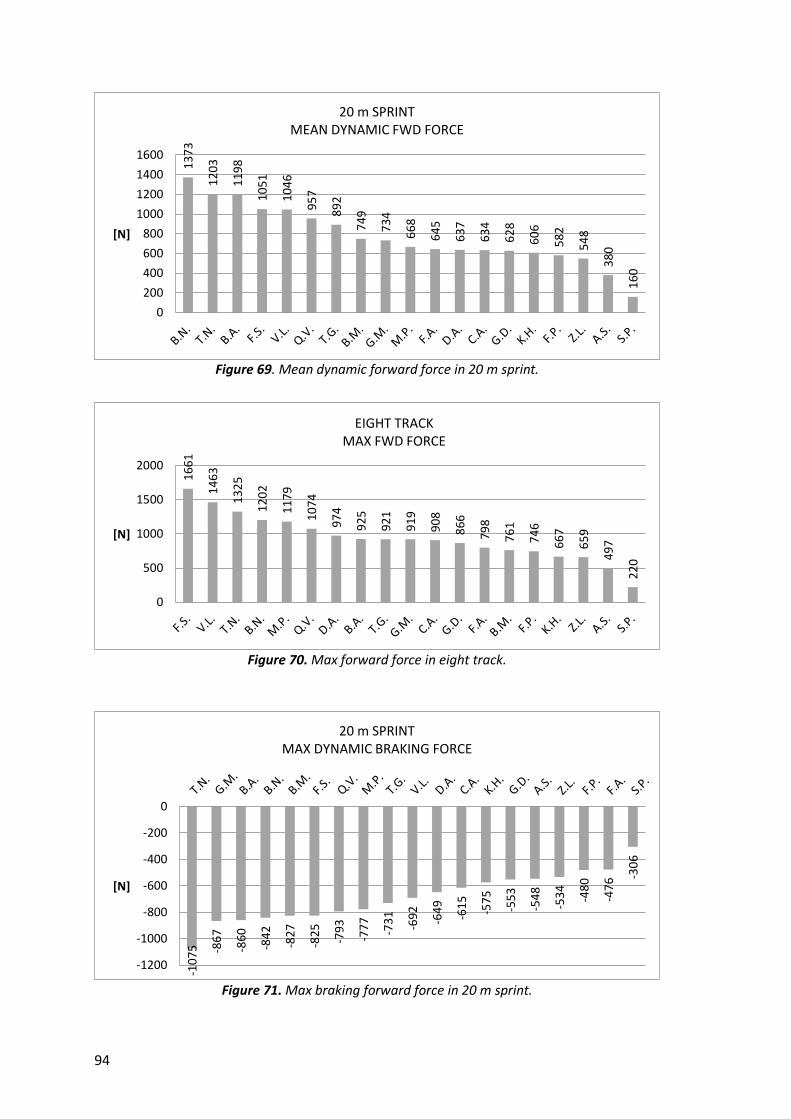
94
Figure 69. Mean dynamic forward force in 20 m sprint.
Figure 70. Max forward force in eight track.
Figure 71. Max braking forward force in 20 m sprint.
13
73
12
03
11
98
10
51
10
46
95
7
89
2
74
9
73
4
66
8
64
5
63
7
63
4
62
8
60
6
58
2
54
8
38
0
16
0
0
200
400
600
800
1000
1200
1400
1600
[N]
20 m SPRINTMEAN DYNAMIC FWD FORCE
16
61
14
63
13
25
12
02
11
79
10
74
97
4
92
5
92
1
91
9
90
8
86
6
79
8
76
1
74
6
66
7
65
9
49
7
22
0
0
500
1000
1500
2000
[N]
EIGHT TRACKMAX FWD FORCE
-10
75 -8
67
-86
0
-84
2
-82
7
-82
5
-79
3
-77
7
-73
1
-69
2
-64
9
-61
5
-57
5
-55
3
-54
8
-53
4
-48
0
-47
6 -30
6
-1200
-1000
-800
-600
-400
-200
0
[N]
20 m SPRINT MAX DYNAMIC BRAKING FORCE

95
The maximum and mean dynamic forward force rankings generally agree. Two of the 3.5
points (B.A., F.S.) are in both cases among the first five places; the exception is M.P. that
situates at the 16th place in the max force, and in the 10th place in the mean force. The reason
can be found in the comparison between the isometric force, in the next paragraph. The
braking force ranking agrees with the forward force ones.
The results for the rotation and eight track are represented in the following graphs
(figures 72, 73).
Figure 72. Angular velocity values in the rotation test, sorted by the left side.
Figure 73. Angular velocity values in eight track, sorted by the left side.
The angular velocity force values for the rotation are, in average, 80% higher than eight
track values: this was expected, since the rotation took place around the Z axis of the
wheelchair-player system on place, while in the eight track the player had to turn around a
41
7
40
3
38
5
34
2
31
6
31
1
30
7
29
9
29
8
29
0
27
0
26
8
26
5
25
7
24
1
23
8
22
4
20
7
18
7
36
4 40
4
36
7
36
8
31
8
30
7
30
5 32
6
28
9
29
6
30
6
23
9 27
6
27
0
26
4
24
5
23
4
20
4
17
5
0
50
100
150
200
250
300
350
400
450
[de
g/s]
ROTATION TESTMAX ANGULAR VELOCITY - LEFT AND RIGHT
Left Right
20
6
20
3
20
2
20
0
19
3
18
3
18
2
18
2
18
0
17
8
17
7
17
2
17
1
16
7
16
6
16
4
15
5
13
8
13
6
23
7
17
6 18
8
19
0
17
1 19
1
16
6
16
0 18
8
15
6 16
8
15
8
16
9
16
7
17
4
16
0
14
2 17
6
12
1
0
50
100
150
200
250
[de
g/s]
EIGHT TRACKMAX ANGULAR VELOCITY - LEFT AND RIGHT
Left Right

96
fixed point, external to his system and coming from a forward acceleration phase. The
situation was different also because, in the rotation test, the subject had to equally use his
arms, in different directions, to execute the movement while in the eight track, turning
around a cone, while an arm is pushing the opposite is braking. In general, players do not
present high differences between the left and right side performance.
The following graphs (figures 74, 75, 76) show the push frequency ranking in a 20 m sprint
and time rankings in 20 m and eight track.
Figure 74. Push frequency in 20 m sprint.
Figure 75. Mean time in 20 m sprint.
2,6
72
2,5
91
2,5
37
2,3
09
2,3
02
2,2
91
2,2
73
2,2
17
2,1
58
2,0
46
2,0
40
2,0
01
1,9
19
1,9
07
1,8
99
1,7
68
1,7
09
1,6
85
1,1
78
0,0
0,5
1,0
1,5
2,0
2,5
3,0
[Hz]
20 m SPRINTPUSH FREQUENCY
6,2
2
6,6
2
6,7
6
6,9
4
6,9
7
7,0
5
7,3
5
7,3
7
7,4
2
7,4
7
7,6
6
7,8
7
8,0
5
8,1
9
8,2
0 9,2
2
9,3
0
9,5
7
12
,16
0
2
4
6
8
10
12
14
[s]
20 m SPRINTMEAN TIME

97
Figure 76. Mean time in eight track.
Time rankings of 20 m sprint do not completely correspond to the ranking of the mean
forward force. For example, M.P. has a low position in the force ranking, but he is at the
second place in time; G.D. and Z.L. present similar situations. This could mean that their
movement are very efficient since with low forces they can reach low times: this could also
mean that with the application of a higher force, they could even reduce their time. On the
contrary, B.N. exerts the highest dynamic forward force, but places in the middle of the time
ranking: this could mean that his movement is inefficient since his high force dissipates fast.
In fact, his push frequency places in the middle of the ranking. The comparison with the
isometric force is needed.
It is worth to notice that players that were in the last part of the ranking for the 20 m
force values like M.P. and Z.L., position in the first places in the angular velocity results: this
means that a player cannot be evaluated from only one performance, but the whole athletic
actions must be taken into account. These results also underline which are the points of
force of the team: some people can express a higher acceleration and thus be strong in a
sprint to the goal line, others can express a higher angular velocity thus being able for
example, to move on the court avoiding the opponents’ blocks.
There are some differences in the maximum forward force expressed during a 20 m
sprint and in an eight track, as shown in figure 77. Most of people locates in the bisector
line; some (M.P., F.S.) express a higher force during the 20 m sprint, others (B.A., B.N.,T.N.,
T.G, Q.V., B.M.) express more than 20% of force in the eight track. This could be explained
with the fact that an eight track is more similar to a game situation respect to a sprint, and
maybe the motivation is higher.
9,4
4
9,5
3
9,6
5
9,8
4
9,8
5
10
,45
10
,52
10
,68
10
,76
10
,84
10
,88
10
,96
11
,09
11
,48
11
,57
12
,52
12
,67
13
,61 16
,51
0
5
10
15
20
[s]
EIGHT TRACK MEAN TIME

98
Figure 77. Max eight track force vs max 20 m forward force. The grey line represents the bisector.
The following graph (figure 78) shows the relation between the point of classification of
each player and his mean FWD force in the 20 m sprint. The tendency line, obtained with a
three order polynomial fit, reveals that there is a correlation between the point and the
explicated force: the 3.5 points express double force respect to the 0.5 points. Nevertheless,
some situations must be noticed: the 3.5 points express, on average, the same force of the
2 and 2.5 points (a linear regression, as done for the isometric push forward force, was
avoided since it could not show this fact). Assuming that the increment between points
should be linear, this means that the aim is to increase the pendency of the last part of the
curve, by improving the performance of the higher points.
Figure 78. Point of classification vs mean FWD force in a 20 m sprint. Dashed line: tendency
line.
S.P.A.S.
C.A.
M.P.
Z.L.
K.H.F.P.
F.A.
G.D.
D.A.
G.M.
B.M.
T.G.
Q.V.
F.S.
V.L.
B.A.
T.N.
B.N.
0
200
400
600
800
1000
1200
1400
1600
1800
0 200 400 600 800 1000 1200 1400 1600 1800
Max
20
m F
WD
Fo
rce
[N
]
Max 8Track Force [N]
B.N.T.N.
B.A.V.L.
F.S.Q.V.T.G.
B.M.
G.M.
D.A.
G.D.F.A.
F.P.
K.H.
Z.L.
M.P.
C.A.
A.S.S.P.
0
200
400
600
800
1000
1200
1400
1600
1800
2000
0 0,5 1 1,5 2 2,5 3 3,5
Me
an 2
0 m
FW
D F
orc
e [
N]
Classification point

99
5.4.4 Dynamic Vs isometric force values In comparing the results found for the dynamic tests with the isometric tests, it is worth
making some considerations. The graph in figure 79 represents the isometric push forward
force vs the mean 20 m forward force. The tendency line reveals that the mean dynamic
force is 2.21 times higher than the isometric push force.
Figure 79. Isometric push forward force vs mean forward force in 20 m sprint.
Most of players are close to the regression line, but in some cases the difference between
dynamic and isometric values is important. Subjects that collocate under the line exert more
force in isometric contraction, subjects above the line are more skilled in dynamic
conditions. People as M.P. and Z.L. potentially have the higher isometric force values, but
they do not express them in dynamic conditions: this can be related to an inefficient pushing
technique, or to a wrong wheelchair setting. Their training should be focused on the
improvement of performance in dynamic conditions, and eventually in a revision of their
wheelchair dimensions. People as B.N. on the contrary, present a high dynamic force and
their work seems to be more efficient. This could mean that increasing the isometric force
with focused force training, their dynamic performance could further improve.
The reason why dynamic values are more than double respect to the isometric force
values might be explained with the fact that in the dynamic test, many inertial factors
influence the performance: these do not occur in the isometric test. The player starts from
a still position and after some pushes, he reaches a regime trend. The mean forward force
was calculated by considering the higher peak of acceleration for each push, and making an
average of them. Nevertheless, these peaks does not correspond to a situation in which the
subject starts from a static position as it is for the dynamic test: he comes from a positive
S.P.
F.A.
D.A.
K.H.
F.P.
A.S.
G.M.
B.N.
B.M.
T.G.Q.V.
G.D.
T.N.
Z.L.
F.S.
B.A.
C.A. M.P.
y = 2,2128x
0
200
400
600
800
1000
1200
1400
1600
0 100 200 300 400 500 600
Me
an 2
0 m
FW
D F
orc
e [
N]
Isometric Push FWD Tot Force [N]

100
acceleration that gives him inertial force. For this reason, the situation within a dynamic
sprint which is more similar to the isometric test condition, is the beginning of the exercise,
when the player exerts the first push. The peak of the first push is actually lower than the
following since it is not affected by inertial factors (figure 80).
Figure 80. Forward acceleration in a 20 m sprint (T.N.); black circle: first positive peak.
Table 9 shows the comparison
between the first peak of force in
dynamic situations, the mean peaks
value and the isometric force value.
The force in the first peak was
obtained through an average between
the first positive peak values of the
three trials of the 20 m sprint forward
acceleration (multiplied for the body
weight), for each player. Figure 81
represents the linear regression of the
isometric force values vs first peak of
force, and of isometric force values vs
mean dynamic force.
INITIALS
20 m SPRINT
FIRST PEAK FORCE [N]
ISO PUSH FWD FORCE
TOT [N]
20 m SPRINT MEAN FWD FORCE [N]
A.S. 234,59 268,95 380,29 B.A. 565,81 452,00 1197,97 B.N. 441,80 324,30 1372,90 B.M. 254,06 335,20 748,89 C.A. 255,43 318,90 633,90 D.A. 262,15 198,10 636,83 F.P. 243,04 250,00 582,44 F.A. 284,40 195,00 644,88 F.S. 290,50 469,30 1051,46 G.D. 336,91 391,80 627,94 G.M. 295,11 271,10 734,08 K.H. 226,10 218,60 606,26 M.P. 421,16 563,83 667,58 Q.V. 396,69 384,03 957,01 S.P. 85,97 148,30 159,95 T.G. 309,06 341,07 892,39 T.N. 386,71 417,83 1203,17 V.L. 374,47 83,77 1046,06 Z.L. 313,17 457,47 548,38
Table 9. Force values from the first push in 20 m; isometric push forward force; mean dynamic
forward force.

101
Figure 81. Isometric push forward force VS mean 20 m forward force (light grey symbols,
dashed line); Isometric push forward force VS first push force (grey circles, solid line).
The first positive acceleration values found in the 20 m sprint are comparable to the
isometric force, more than the mean force values: the linear regression shows a high
correspondence (92%) between the two trends. Some differences occur, since the first push
of the 20 m sprint does not come from an isometric contraction, the friction of the floor is
lower than the one received during the isometric test, the position of arm and trunk are
different. In conclusion, this result give an additional confirm that the high difference
between isometric and dynamic values is owed to inertial factors.
5.4.5 Match The results coming from the match analysis are limited to eight athletes playing the first
and the second time, and represented in figure 82. The first observation is that the
maximum forward acceleration values were higher than the values found in the dynamic
tests: this was expected, since the match creates different game situations and adds the
motivation. Another observation is that each player has his different distribution of peaks.
y = 0,9162x
y = 2,2128x
0
200
400
600
800
1000
1200
1400
0 100 200 300 400 500 600
[N]
Isometric Push FWD Tot Force [N]
First peak force 20 m Mean FWD force 20 m
Lineare (First peak force 20 m) Lineare (Mean FWD force 20 m)
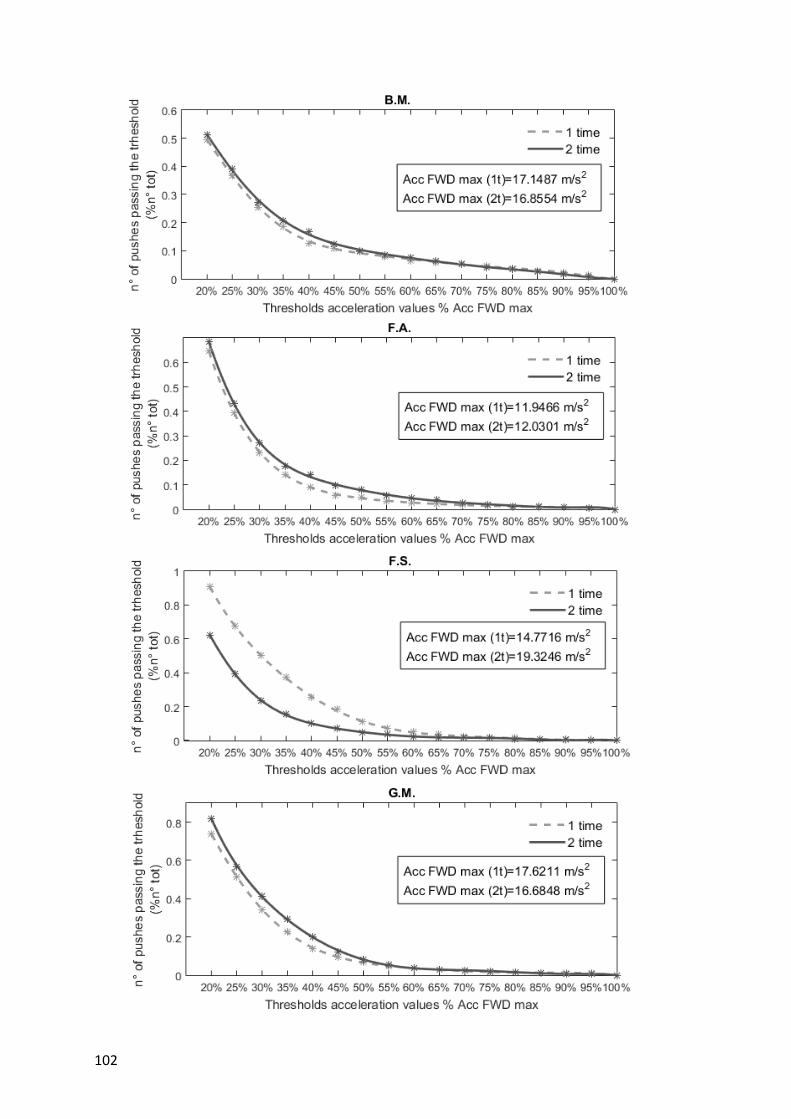
102

103
Figure 82. Cumulative distribution of the eight players of the match. The first time is the dashed line; second time is the solid line.
.

104
The rapid decrease (high slope) of the initial part of the curve, observed in all cases, shows
that players mostly work at very low acceleration: their pushes are on the majority lower
than the maximum.
Another relevant factor is the percentage at the 20% threshold: values at the 0.8 (T.G., G.M.)
indicate that the majority of pushes are more than 20% of the maximum acceleration. 0.6
or lower values, observable in most cases (B.M., M.P., K.H., T.N.) indicate that the 40% of
pushes are at less than 20% of the max acceleration: this could mean that the player does
not work at his best, and he should improve his court performance.
The difference between first and second time trends is generally low: curves are
comparable, in particular for the higher values of acceleration (more than 50%). F.S. is the
only case who reached very high values of acceleration in the first time (more than 0.9 of
pushes were more than 20% of the max acceleration) and low values in the second (0.5):
this might be imputable to a lack of physical resistance in the second time. Moreover,
maximum acceleration values in the first and second time are comparable, apart for F.S. and
T.N. who both present higher values in the second time.
A future development of these measures is the fixation of inertial sensors on wheel axles
(as explained in the previous paragraphs) during a match, to determine the total distance
covered by the wheels. Analysis of the covered distance made for eight tests gave results
that are exportable in the analysis of an entire match, in which the path is unknown and the
situations are more complex. It is important to acquire the signal coming from both wheels,
since the obtained distance may have differences caused by the prevalence of rotations in
left or right direction.
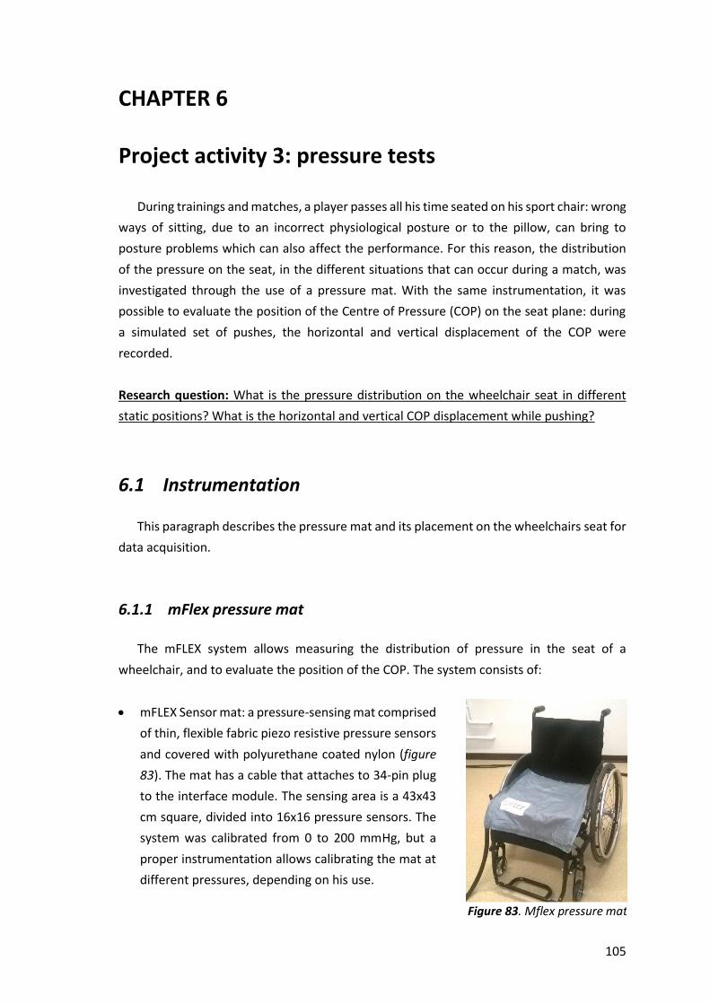
105
CHAPTER 6
Project activity 3: pressure tests
During trainings and matches, a player passes all his time seated on his sport chair: wrong
ways of sitting, due to an incorrect physiological posture or to the pillow, can bring to
posture problems which can also affect the performance. For this reason, the distribution
of the pressure on the seat, in the different situations that can occur during a match, was
investigated through the use of a pressure mat. With the same instrumentation, it was
possible to evaluate the position of the Centre of Pressure (COP) on the seat plane: during
a simulated set of pushes, the horizontal and vertical displacement of the COP were
recorded.
Research question: What is the pressure distribution on the wheelchair seat in different
static positions? What is the horizontal and vertical COP displacement while pushing?
6.1 Instrumentation
This paragraph describes the pressure mat and its placement on the wheelchairs seat for
data acquisition.
6.1.1 mFlex pressure mat
The mFLEX system allows measuring the distribution of pressure in the seat of a
wheelchair, and to evaluate the position of the COP. The system consists of:
mFLEX Sensor mat: a pressure-sensing mat comprised
of thin, flexible fabric piezo resistive pressure sensors
and covered with polyurethane coated nylon (figure
83). The mat has a cable that attaches to 34-pin plug
to the interface module. The sensing area is a 43x43
cm square, divided into 16x16 pressure sensors. The
system was calibrated from 0 to 200 mmHg, but a
proper instrumentation allows calibrating the mat at
different pressures, depending on his use.
Figure 83. Mflex pressure mat

106
Interface module: the electronic communicator between the mat sensors and the
computer. The interface module connects to the computer via USB cable, and it
needs a constant charging, supplied with the system.
Computer software to view, register and export file information gathered by the
sensors. The software automatically saves the file of acquisitions with
.mfl extension. On the output, the square of the mat is visualized on real time
(figure 84); after a video recording, also the statistical data about the pressure
distribution with their time plot are available.
Figure 84. mFlex software.
6.1.2 Mat placement The subject was asked, with some help, to move from his wheelchair, to easily place the
mat in the correct way on his seat. The pillow was removed, to better position the mat on it
minimizing folds, and rolling its extremities up the sides of the pillow. The mat’s cable was
kept on the front-right side, to avoid any impediment for the movement. The
instrumentation (PC, interface module) was placed in front of the athlete, to have no
obstacle with the cables, and to allow him seeing the output on the PC screen during the
exercises. The subject was asked to prepare himself as if he had to play, with all the straps
and gloves. Once the mat was positioned, a set of acquisition to track the edge of the pillow
in the mat, was executed: this should avoid an incorrect interpretation of data for the
presence of artefacts. Then, the subject could execute the whole set of exercises.

107
6.2 Methods
Pressure tests were executed for 14 of the 19 participants to the project, plus one extra
player (P.S.) who made available for the test.
6.2.1 Tests description Two kind of test were executed: a static test, to see the distribution of pressure in
different positions, and a dynamic test to analyse the displacement of the centre of pressure
(COP) during a simulated set of pushing.
6.2.1.1 Static tests
The subject was asked to execute a set of static movements. Starting from a normal
sitting position, he had to move backward, forward, right and left, imaging during each
situation, to have the need of picking up the ball from the floor (this was asked to avoid
unnatural movements). Each position was maintained for 5 seconds, and between two
different movements he always passed through the rest position, staying for 5 seconds:
1. normal rest position, with hands on wheels (5s)
2. forward position (5s) (figure 84a) + rest position (5s)
3. backward position (5s) (figure 84b) + rest position (5s)
4. left position (5s) (figure 84c) + rest position (5s)
5. right position (5s) (figure 84d) + rest position (5s).
The whole set was recorded as a video in the acquisition software.
a) b)

108
c) d)
Figure 84. Set of positions for the static test. a) Forward; b) backward; c) left; d) right.
6.2.1.2 Dynamic tests
This kind of test simulated a real set of pushing. A wooden thickness with a plastic mat
above it were placed under the rear castors to suspend them, allowing the wheels not to
touch the ground. To create a friction for wheels, a resistance was simulated with two plastic
mats, one for each wheel, placed in contact with the floor and the wheel. Starting from the
normal rest position, the athlete was asked to execute a number of pushes, then to return
to the rest position:
1. normal rest position (5s);
2. 10 pushes;
3. normal rest position (5s).
The whole set was recorded as a video by the software.
6.2.2 Data analysis The data extracted from each static test were the graphical distribution of pressure on
the seat, for the five assumed positions: normal, forward, backward, left and right. The video
sampling frequency was 5 Hz, so each position was assumed, approximatively, for 25
samples. Excluding the first samples in which the subject came from the previous position
and is not well positioned, a screenshot of the distribution when the position is graphically
stable, was chosen.
For the dynamic tests, the position of the COP was evaluated. The software records, for
each video sample, the horizontal and vertical position of the COP (in cm), considering the
zero as the exit of the cable, which is always shown on the PC screen (figure 85). The lower

109
base of the output square always correspond to the seatback, the upper base correspond
to the knees.
Figure 85. Mat pressure distribution, COP vertical and horizontal coordinates.
For each dynamic test, the maximum vertical and horizontal displacement within the set
of pushes was extracted by considering the time fit given by the output. For both the
horizontal and vertical centre trend, the difference between maximum and minimum values
within the pushes, was extracted.
6.3 Results
The results must be interpreted taking into account the protocol for the data collection:
the graphical output pressure distribution, indeed, can be influenced by some artefacts
(figure 86).
Figure 86. Artefacts in a graphical output.

110
Therefore, the main problem within the mat placement was the presence of some folds of
the mat: its adaptation to the pillow creates zones in which the pressure is positive. This
happened because mat dimensions are higher than the dimensions of the common
rugby wheelchair pillows, and obligates the mat itself to be rolled around the pillow. Other
artefacts could be generate by straps that players use to fix them to the chair, which in some
cases interfere with the mat, or to additional cushioning around or under the pillow, added
to a more comfortable position.
Despite the presence of artefacts, static results highly differ among the tested subjects:
this is owed to many factors. Firstly, in relation to the type of cushion (thickness, dimensions,
material, overuse), the distribution and the peak of pressure vary. Then, physical structure
of the person determines larger or narrower pressure distribution. Generally, the sensor
corresponding to ischial tuberosities show higher values of pressure. For some subjects this
values are low (40 mmHg), for others they reach the saturation (200 mmHg). With the left
and right movements, the corresponding values increase. An example is shown in figure 87.
Figure 87. Pressure distribution in static test (F.A.); centre: rest position.

111
It is possible to notice that rest pressure distribution is symmetrical, but shows saturation
values in correspondence to ischial tuberosities. The left movement creates a higher left
peak in the left ischial tuberosity and lower values in the right one, and this happens
symmetrically for the right movement. In the forward position, the same zones have lower
values than in rest position, without reaching the saturation. In backward movement, the
distribution is very close to the rest one: the subject, indeed, does not have the full control
of his trunk and so his backward movements are very limited.
In other cases, the higher pressure values correspond to the contact of the thighs with
the edge of the pillow. An example is represented in figure 88.
Figure 88. Pressure distribution in static test. (N.B.); centre: rest position.
In this case, the non zero values are more spread, and the whole pressure distribution
assumes, on average, higher values than the previous case (figure 87). The movements are
wider since the subject have the control of his trunk: the forward and backward position
highly differ from the rest position. The rest pressure distribution is quite symmetrical, apart
112
for a peak of pressure in the distal part of the left thigh, which reaches saturation values not
only in forward and left position, but even when the movement is backward or to the right.
In this case, even in dynamic conditions, that zone maintains the same saturation value. This
could be associated to a wrong posture and should be further investigated: a limited region
with constant and high pressure value, could produce tissue damage.
There is no agreement on a pressure threshold for tissue damage. The existent studies
were executed for daily wheelchair; some researchers indicated that tissue damage occur
with a peak of pressure (PP) of 45 mmHg with friction, and 67.5 mmHg without friction.
Nevertheless, many studies recorded PP greater values than the tissue damage thresholds
reported in literature [30,31,32]. Differences between static and dynamic seat interface
pressures were recorded: PP in static seat was lower than in dynamic tests. According to the
research by Kalpen [32], reduced PP was found with an air-filled cushion compared with
foam. Static PP was 18kPa (135mmHg) on the air cushion and 25kPa (187.5mmHg) on foam.
The maximum PP was approximately 40% greater for the foam cushion than for the air.
Kernozek found PP values of 16.2 kPa (121.5 mmHg) in static seat, and 20.3 (152.3) in
dynamic seat. The values found in this work are sometimes higher. Apart for Q.V, K.H, F.P,
G.D., all the subjects presented PP saturation values (200mmHg) in at least one of the static
positions: this mean that those values can be even higher. This could be associated, as
reported in literature, to the foam cushion that is usual for rugby wheelchairs and could be
moreover, a pressure able to induce tissue damages. Nevertheless, the cited studies refer
to daily use wheelchairs, in which tissue damage is owed to the fact that the user sits for
long time in the same position, and with a pressure distribution that varies only in relation
to limited movements. This situation highly differs from the large range of movement that
a rugby player exhibits during a match: in this case, pressure distribution varies primarily
because of the propulsion movement, and the risk for tissue damage should be lower since
it does not involve long times in the same position. The presence of eventual zone with
constant saturation values should be further examined.
From the data analysis of the dynamic test, the maximal horizontal and vertical
displacement of the COP (figure 89) during a set of 10 pushes, were extracted and
represented in table 10. These values give information about the personal pushing
technique. The COP position is calculated by the software as a weighted average between
the sensors’ pressure values: therefore, its position in the mat square is influenced by
artefacts. Nevertheless, the displacement is not affected by this problem, since it was
calculated as a difference, and its absolute position within the square is not relevant.

113
No correlation between the point of classification and the COP displacement were found:
this mean that the COP displacement is related to the personal pushing technique, to the
posture in the chair, the pillow and many other factors and cannot be compared.
The use of the trunk itself, is not a discriminant factor since players who fully use their
trunk (as M.P, Q.V) have comparable values to those who do not have a full control of their
trunk (T.G., K.H.). The higher values were recorded from G.M. (2.5 point of classification):
visually, his pushing technique consists of deep movements, and he has the total control of
his trunk. The lower values were recorded for F.A. (0.5): he does not have the control of his
trunk, and for his physical characteristics, his movement are not wide.
In conclusion, the mat used in this study was not appropriate for these tests: its
dimensions fits in a daily use wheelchair seat, but rugby chairs seat is more narrow.
Moreover, the presence of straps and border of the seat creates many artefacts and the
consequent difficulty to data interpretation, since is not always clear if a zone is generated
by the body pressure distribution or by other factors. Moreover, the mat must be calibrated
at higher pressures since with the maximum scale value at 200 mmHg, all player reached
the saturation so the correspondent values are probably higher.
DELTA COP [cm]
INITIALS POINTS HORIZONTAL VERTICAL
B.A. 3,5 13,39 3,88
B.N. 2 2,94 2,96
B.M. 2,5 1,90 5,92
F.P. 1 3,35 2,62
F.A. 0,5 0,75 0,65
G.D. 1,5 2,21 1,83
G.M. 2,5 16,37 10,44
K.H. 1 5,54 3,64
M.P. 3,5 4,81 4,43
P.S. 1,5 3,33 0,99
Q.V. 2,5 4,29 7,71
T.G. 1,5 4,29 4,46
T.N. 2,5 7,60 7,33
V.L. 2,5 4,59 5,07
Z.L. 2,5 2,84 2,61
Table 10. Horizontal and vertical displacement of the COP during dynamic
tests.
Figure 89. Displacement of the COP during dynamic tests (G.M.).

114

115
CHAPTER 7
7.1 Conclusions
A Wheelchair Rugby player is the sum of many different aspects. The present work is
comprised in a wider project which investigates this high number of features. Isometric
measures of unilateral and bilateral pushing forward, and shoulder/elbow
flexion/extension, combined with medical investigations, allowed assessing the presence of
asymmetries in contralateral joints, and defining sportive and therapeutic training based on
each need. Moreover, they allowed identifying situations at risk of infortune, and
programming the recovery of the damaged function to avoid eventual relapses owed to a
premature return to the sportive activity.
The tests of 20 m sprint underlined the presence of different pushing techniques,
determined the push frequency, the maximum force exerted in a dynamic situation.
Rotation tests identified the ability of spinning, and the analysis of eight track showed that
some people are more skilled in spinning than in accelerating. From all tests, force rankings
were complied, to give a general view of the present situations, and determine which are
the points of force of the team.
Forces in dynamic tests were compared with isometric forces, underlining the fact that
in dynamic conditions, inertial effects play an important role on force generation. In both
cases, the correlation between force and point of classification is not always linear: this
means that each player could improve his force with a proper training.
Pressure tests on wheelchair seats underlined the presence of high peaks of pressure if
related with literature studies: nevertheless, the mat was not appropriate for the present
study for its dimensions and the consequent presence of artefacts.
7.2 Future developments
Biomechanical analysis performed in this work will continue in the next team meetings.
Meanwhile, players are undergoing a program of training based on the improvement of
force, resistance and skills related to the game.
Isometric force tests will be repeated, to determine the efficacy of sport training, with
the adoption of a more standardize acquisition protocols: all subjects must perform the

116
exercise with the same angles of shoulder, elbow and trunk flexion/extension, same position
for wristbands, and minimizing any force compensation effect that could distort measures.
Dynamic tests will be repeated with the same conditions. Wheel sensors will be placed
also during a match, to obtain the total distance covered by players. Moreover, the
application of a heart rate monitor together with an inertial sensor could synchronize heart
rate with forward acceleration and give more information about court performance.
Further analysis comprise the study of trunk movement: with an inertial sensor it is
possible to determine trunk angles and acceleration in a sprint, and synchronize it with the
forward acceleration of the system. This allow understanding if some oscillations in the
forward acceleration trend are owed to the trunk.
The project of a rugby wheelchair ergometer is in program, to allow executing metabolic
tests in conditions that are more similar to the real situations, instead of an arm ergometer;
moreover, it would make possible the MoCap analysis of the propulsion.
The realization of an inclining platform with force plates will allow determining the spatial
localization of the centre of mass of the wheelchair-player system. Starting from that, a
study on the stability of the system will be executed.
The use of a Smart Wheel could have different applications: as example, in dynamic
conditions, for the synchronization of force signals on the handrim with the forward
acceleration, and on the ergometer, to perform test also with the MoCap for a deeper and
complete study.
The analysis of performance is carrying on with investigations about strikes: the
understanding of the maximal loads applied on the wheelchairs, allows starting a FEM study
which should end in the proposal of modifications to improve the frame structure.
The biomechanical analysis performed in this study, moreover, wanted to increase the
knowledge about Wheelchair Rugby, which lacks of research studies: this sport is still not
well known.
Sport for people with physical disability can help them finding an autonomy and a higher
knowledge of their potentialities, which are helpful also in their daily activities. For this
reasons it is necessary to continue the study, and to spread information about Paralympic
sports which are as important as sports for able-bodied. Moreover, in Paralympic sports,
where the personal difficulty is higher, the dedication and the final satisfaction could be
even greater. As Pierre de Coubertin, founder of the modern Olympic Games, stated: “The
sport goes looking for the fear to dominate it, the effort to surmount it, the difficulty to win”.

117
REFERENCES
[1] International Wheelchair Rugby Federation. IWRF Classification Manual. 3rd Edition;
Revised 2015.
[2] Athens 2004 Organising Committee for the Olympic Games. The Paralympic Games from
1960 to 2004.
[3] International Wheelchair Rugby Federation. International Rules for the Sport of
Wheelchair Rugby 2015.
[4] Official site of IWRF: http://www.iwrf.com/
[5] LHV van der Woude, HEJ Veeger, AJ Dallmeijer, TWJ Janssen, LA Rozendaal.
Biomechanics and physiology in active manual wheelchair propulsion. Medical Engineering
& Physics 2001; 23: 713-733.
[6] CC Campbell, MJ Koris. Etiologies of shoulder pain in cervical spinal cord injury. Clin
Orthop Relat Res 1996; 322:140-5.
[7] IH Sie, RL Waters RH Adkind, H Gellman. Upper extremity pain in the postrehabilitation
spinal cord patient. Arch Phys Med Rehabil 1992; 73:44-8.
[8] Y Vanlandewijck, DTheisen, D Daly. Wheelchair Propulsion Biomechanics: Implications
for Wheelchair Sports. Sports Med 2001; 31(5):339-67.
[9] American Colleague of Sports Medicine. Resource manual for guidelines for exercise
testing and prescription. Philadelphia: Williams & Wilkins, 1993. 2nd ed.
[10] X Devillards, P Calmels, B Sauvignet, A Belli, C Denis, C Simard, V Gautheron. Validation
of a new ergometer adapted to all types of manual wheelchairs. Eur. J. Appl. Physiol. 2001;
85, 479-485.
[11] LHV Van der Woude, G De Groot, AP Hollander, GJ Van Ingen Schenau, RH Rozendal.
Wheelchair ergonomics and physiology testing of prototypes. Ergonomics 1986; 29(1):1561-
73.
[12] KT Assato, RA Cooper, RN Robertson, JF Ster. Smartwheels: development and testing of
a system for measuring manual wheelchair propulsion dynamics. IEEE Trans Biomed Eng
1993; 40: 1320-4.
[13] HEJ Veeger, LHV van der Woude, RH Rozendal. Load on the upper extremity in manual
wheelchair propulsion. J Electromyogr Kinesiol 1991; 1 (4): 270-80.
[14] HW Wu, FC Su. An instrumented wheel for the kinetic analysis of wheelchair propulsion.
J Biomed Eng 1998; 120:533-5.
[15] K Roeleveld, E Lute, HEJ Veeger, T Gwinn, LHV van der Woude. Power output and
technique of wheelchair athletes. Adapt Phys Act Quart 1994; 11(1):71–85.
[16] HEJ Veeger, EM Lute, K Roeleveld, LHV van der Woude. Differences in performance
between trained and untrained subjects during a 30-s sprint test in a wheelchair ergometer.
Eur J Appl Physiol Occup Physiol 1992;64(2):158-64.

118
[17] HEJ Veeger, LHV van der Woude. Force generation in manual wheelchair propulsion. In:
XIII Southern Biomedical Engineering Conference, 1994:779-82.
[18] HEJ Veeger, LHV van der Woude. Force generation in manual wheelchair propulsion. In:
H Van Coppenolle, Y Vanlandewijck, J Simons, et al., editors. Proceedings of the First
European Conference on Adapted Physical Activity and Sports: a white paper on research
and practice; 1994 Dec 18-20: Leuven. Leuven: Acco, 1995: 89-94.
[19] LY Guo, KD Zhao, FC Su, KN An. Moment generation in wheelchair propulsion. Proc Inst
Mech Eng H. 2003;217(5):405-13.
[20] WJ Rankin, AM Kwarciak, WM Richter, RR Neptune. The influence of altering push force
effectiveness on individual muscle demand during wheelchair propulsion. J Biomech. 2010;
43(14): 2771–2779.
[21] AJ Dallmeijer, LHV van der Woude, HEJ Veeger, AP Hollander. Effectiveness of force
application in manual wheelchair propulsion in persons with spinal cord injuries. Am J Phys
Med Rehabil 1998; 77 (3): 213-21.
[22] AJ Dallmeijer, YJ Kappe, HEJ Veeger, TW Janssen, LH van der Woude. Anaerobic power
output and propulsion technique in spinal cord injured subjects during wheelchair
ergometry. J Rehabil Res Dev 1994; 31 (2): 120-8.
[23] FCT van der Helm, HEJ Veegert. Quasi-static analysis of muscle forces in the shoulder
mechanism during wheelchair propulsion. J Biomech. 1996;29(1):39-52.
[24] CC Usma-Alvarez, FK Fuss, A Subic. Effects of rugby wheelchair design on output velocity
and acceleration. Procedia Engineering 2011. 13: 315–321.
[25] YC Vanlandewijck, AJ Spaepen, RJ Lysens. Wheelchair propulsion efficiency: movement
pattern adaptations to speed changes. Med Sci Sports Exerc 1994; 26 (11): 1373-81.
[26] AJ Spaepen, YC Vanlandewijck, RJ Lysens. Relationship between energy expenditure
and muscular activity patterns in handrim wheelchair propulsion. Int J Indust Ergon 1996;
17: 163-73.
[27] HEJ Veeger, LHV van der Woude, RH Rozendal. Wheelchair propulsion technique at
different speeds. Scan J RehabilMed 1989; 21: 197-203.
[28] LHV van der Woude, HEJ Veeger, RH Rozendal. Propulsion technique in hand rim
wheelchair propulsion. J Med Eng Tech 1989; 13: 136-41
[29] YC Vanlandewijck, AJ Spaepen, M Heister. Maximal exercise responses and manual
wheelchair propulsion: cardiorespiratory and movement pattern adaptations to slope and
velocity changes. In: Van Coppenolle H, Vanlandewijck Y, Simons J, et al., editors.
Proceedings of the First European Conference on Adapted Physical Activity and Sports: a
white paper on research and practice; 1994 Dec 18-20: Leuven. Leuven: Acco, 1995: 73-8.
[30] M Kosiak. A mechanical resting surface: its effect on pressure distribution. Arch Phys
Med Rehabil 1976; 57:481-4.
[31] TW Kernozek, JE Lewin. Seat Interface Pressures of Individuals With Paraplegia:
Influence of Dynamic Wheelchair Locomotion Compared With Static Seated Measurements.
Arch Phys Med Rehabil. 1998; 79(3):313-6.

119
[32] Kalpen A, Bochdansky T, Seitz E. The dynamic body pressure distribution in a moving
wheelchair. Workshop MW04: RESNA Conference, June 7-12, 1996.
[33] MNX MEMS and Nanotechnology exchange: https://www.mems-exchange.org
[34] M Andrejasic. Mems Accelerometers. Seminar at Ljubljana University 2008.
[35] G Bellusci, F Dijkstra, P Slycke. Xsens MTw: Miniature Wireless Inertial Motion Tracker
for Highly Accurate 3D Kinematic Applications. Xsens Technologies 2013; Version 29.
[36] F Hintzy, N Tordi. Mechanical efficiency during hand–rim wheelchair propulsion: effects
of base-line subtraction and power output. Clinical Biomechanics 2004; 19:343-349.

120

121
APPENDIX 1
Power Spectral Density
The analysis in the frequency domain is a strong and useful instrument for signal
elaboration. In fact, for some kind of signals, time description can be insufficient to
understand their properties. In this work, the calculation of Power Spectral Density (PSD) is
an important mean to extract some characteristics of the signal that, in time domain, would
have been very difficult to extract.
PSD allows understanding the strength of the variations as a function of frequency: it
shows at which frequencies variations are strong, and at which they are weak. The unit is
energy per frequency. To evaluate PSD it is first necessary to introduce some elements of
signal analysis, as Fourier Transform, energy and power.
Let x(n), −∞ < 𝑛 < +∞ , be a real discrete signal, obtained from the sampling of the
continuous signal x(t); the continuous Fourier Transform of x(n) is:
It is a complex function of the real variable ω (pulsation ω=2π/f, f is the frequency). For a
real signal as x(n) is, the FT has even module and odd phase: it is sufficient to represent its
module and phase in the interval of frequencies of 0-π, or, in terms of frequencies, 0-0.5. In
the continuous domain, with sample frequency Fs, the correspondent intervals are 0-π Fs
for ω and 0-0.5*Fs for frequency.
Given x(n) as a discrete signal with a finite number of samples, n=0,1,…N-1, next the FT it is
possible to calculate the Discrete Fourier Transform with the following expression:
k=0,1,..N-1. It is a complex signal with N samples. From the comparison between FT and
DFT, it is clear that X(k) represents the sequence on N samples of X(ω) in the interval of 0-
2π, as shown in figure 90.
Figure 90. Graphical representation of discrete Fourier Transform of a signal.

122
Let x(t) be a deterministic continuous signal, defined in 0 < 𝑡 < ∞ , its energy is:
Form Parseval theorem considering the Fourier transform (FT) of x(t), being 𝑋(Ω) =
𝐹𝑇(𝑥(𝑡)), energy density is:
And energy spectral density has the following expression:
This expression, integrated in a certain interval of frequencies Ω1- Ω2 , gives the energy
contained in x(t) and associated to those frequencies.
Nevertheless, some signals (stationary and stochastic) have infinite energy, so it becomes
necessary to evaluate power, with this expression:
And Power Spectral Energy:
𝑃(Ω) =1
2𝜋lim𝑇→∞
1
2𝑇| ∫ 𝑥(𝑡) 𝑒−𝑗Ω𝑡 𝑑𝑡
+𝑇
−𝑇
|
2
= lim𝑇→∞
1
2𝑇𝐸
This expression, integrated in a certain interval of frequencies Ω1- Ω2, gives the power
contained in x(t) and associated to that band.
The literature offers many instruments to calculate PSD: parametrical methods, based
on FT (indirect methods using the autocorrelation function, or direct methods), or non
parametrical, based on the use of models. In this work, PSD was calculated with the direct
method of the periodogram.
The formulas to calculate PSD, as shown in the previous expression, implicates the
evaluation of energy and its infinite limit: since the signal x(t) is not defined in an infinite
number of samples, an estimator is defined, as:
In a practical field, this value is calculated through the Discrete Fourier Transform (DFT):
𝑃𝐸𝑅(𝑘) = 1
𝑁 |𝐷𝐹𝑇[𝑥(𝑛)]|2 =
1
𝑁 |∑ 𝑥(𝑛)
𝑁−1
𝑛=0
𝑒−𝑗2𝜋𝑁
𝑛𝑘|
2
= 𝑃𝐸𝑅(𝜔) |𝜔=
2𝜋𝑁
𝑘
k=0,1,…N-1.

123
In this work, in Matlab environment, PSD of the acceleration signal was obtained via the
Matlab function for the fast Fourier Transform fft(x).
APPENDIX 2
Matlab code
2.1 Peak detection for forward acceleration analysis This appendix contains the data analysis, with Matlab R2015a, performed for signal of
forward acceleration in 20 m sprint tests, with the importing of text file and peak detection
algorithm.
close all clc clear all
%% Import data from text file % Initialize variables. filename = 'C:....\MT_00200108_000-000_00341101.txt'; %file path delimiter = '\t'; startRow = 6;
% Format string for each line of text: formatSpec = '%f%f%f%f%f%f%f%f%f%f%f%[^\n\r]';
% Open the text file fileID = fopen(filename,'r');
% Read columns of data according to format string. dataArray = textscan(fileID, formatSpec, 'Delimiter', delimiter,
'EmptyValue’,NaN,'HeaderLines' ,startRow-1, 'ReturnOnError', false);
% Close the text file. fclose(fileID);
% Allocate imported array to column variable names PacketCounter = dataArray:, 1; SampleTimefinish = dataArray:, 2; Acc_X = dataArray:, 3; Acc_Y = dataArray:, 4; Acc_Z = dataArray:, 5; Gyr_X = dataArray:, 6; Gyr_Y = dataArray:, 7; Gyr_Z = dataArray:, 8; Roll = dataArray:, 9; Pitch = dataArray:, 10; Yaw = dataArray:, 11;

124
% Clear temporary variables clearvars filename delimiter startRow formatSpec fileID dataArray ans;
%% Signal elaboration
%Time axis freq=75; %sampling frequency [Hz] n_sample=size(Acc_X,1); %number of samples Ttot=n_sample/freq; %total time of acquisition t_sample=1/freq; %time period t=0:t_sample:Ttot-t_sample; %time axis
Acc=Acc_Y; %Forward acceleration Acc_max=max(Acc); figure plot(Acc) grid on
%Elimination of drift values ind_drift=input('Choose drift indexes: '); %selection of Acc indexes drift=mean([Acc(ind_drift(1)) Acc(ind_drift(2))]) Acc=Acc-drift;
%Selection of acceleration period to analyse period=input('Choose time period to analyse: '); start=period(1); finish=period(2);
%PSD extraction Acc2=Acc(start:finish); %acceleration to analyse N=n_sample; Acc_ft=fft(Acc,N); %Fourier Transform freq_ft=0:freq/N:freq-freq/N; %frequency domain PSD=(abs(Acc_ft).^2)/N; %Power Spectral Density PSD=PSD(1:N/2); freq_ft=freq_ft(1:N/2);
figure plot(freq_ft,PSD) hold on
%Push frequency extraction n_sample2=length(Acc2); [val,ind_ord]=sort(PSD,'descend'); freq_peaks=freq_ft(ind_ord); freq_push=0; for i=1:length(freq_peaks) plot(freq_peaks(i),val(i),'+') ans=input('Accept the peak? y/n ','s'); if ans=='y' freq_push=freq_peaks(i); break end %if end %for hold off
t_push=1/freq_push; %push period Ttot_acc=t(finish)-t(start)+t_sample; M=round(Ttot_acc/t_push); %number of pushes n_acc=round(n_sample2/M); %number of samples for each push

125
figure plot(Acc2) grid on hold on
%Division of acceleration in push periods ind_peaks=[]; peaks=[]; k=1; for i=1:M [c,d]=max(Acc2(k:k+n_acc)); ind_peaks=[ind_peaks d+k-1]; peaks=[peaks Acc2(ind_peaks(i))]; k=k+n_acc+1; if k+n_acc>n_sample2 [c,d]=max(Acc2(k:end)); ind_peaks=[ind_peaks d+k-1]; peaks=[peaks Acc2(ind_peaks(i+1))]; break end %if
end %for
threshold=0.5*max(peaks); hold on plot(threshold*ones(n_sample2),'-b') p=find(peaks>=threshold); plot(ind_peaks(p),Acc2(ind_peaks(p)),'*r')
Acc_mean=mean(peaks(p));
2.2 Covered distance After the extraction of each wheels covered distance with the function integral, following
lines contain the code for the extraction of distance covered by the wheelchair-player
system, represented by the middle point (MP) of the beam connecting wheels axles.
function y=integral(x,start,finish) %%Trapezoidal integral of signal x. %%x: signal to integrate %start, finish: initial and finale indexes of integration
freq=75; %sample frequency n_sample=size(x,1); Ttot=n_sample/freq; t_sample=1/freq; t=0:t_sample:Ttot-t_sample;
x_int=x(start:finish); %signal to integrate
%Integration y(1)=trapz(t(start:start+1),x_int(1:2)); k=1; for i=start:finish-1

126
y_temp=trapz(t(i:i+1),x_int(k:k+1)); y(k+1)=y_temp+y(k); k=k+1; end %for
end %function
%%Calculation of wheelchair covered distance
load('Right_wheel'); %Gyr_right, distance_right load('Left_wheel'); %Gyr_left, distance_left load('MP_Frame'); %Gyr_frame, start and finish indexes, time axis
diameter_inches=input('Insert wheels diameter (inches): ‘);
%generally, 24 or 25 inches diameter=diameter_inches*0.0254;
%Average between wheels angular velocities Ang_vel_med=0; for i=1:length(Gyr_right) Ang_vel_med(i)=(Gyr_right(i)+Gyr_left(i))/2; end %for
%Integration of Ang vel med distance_med=integral(Ang_vel_med,start,finish); distance_med=distance_med/360*(diameter*pi);
%Results figure subplot(211) plot(b,Ang_vel_med(start:finish),'-r') grid on ylabel('Ang vel med [deg/s]') subplot(212) plot(b,distance_med,'b-') hold on plot(b,distance_right,'-b','LineStyle','--') plot(b,distance_left,'-b','Linestyle',':','LineWidth',1.5) xlabel('Time [s]') ylabel('Distance [m]') legend('Average','Right wheel','Left wheel') grid on hold off
distance_tot_right=distance_right(end); %right wheel distance distance_tot_left=distance_left(end); %left wheel distance distance_tot_MP=distance_med(end); %wheelchair middle point (MP)
distance

127

128

129
RINGRAZIAMENTI
Ringrazio prima di tutto la mia famiglia: i miei genitori, i miei fratelli Andrea e Arianna, e
i miei nonni, che mi sono stati vicini in tutti questi anni di studi, dandomi la forza di
continuare nei momenti più difficili, e gioendo assieme a me per ogni piccolo traguardo
raggiunto.
Tutti i miei amici e le persone importanti che ho incontrato in questi anni nella mia
strada, che con la loro pazienza mi hanno supportato sempre ed hanno creduto in me. Senza
i tanti bei momenti passati con loro, staccando dallo studio, non sarei arrivata a questo
traguardo.
Ringrazio il prof. Petrone e tutti i ragazzi incontrati ad Ingegneria Meccanica, assieme ai
quali ho passato questi ultimi mesi imparando molto sia dal punto di vista scolastico che
umano.
Infine i ragazzi del Wheelchair Rugby, grazie ai quali ho scritto questa mia tesi e
conosciuto un mondo che sempre porterò con me.
Maria Laura