Modeling Motion of theLissajous Sand Pendulum

Author: Matthew LomickaFaculty Adviser: David Heddle

Report Submitted: April 19, 2019

Contents

1 Abstract 2

2 Introduction 3

3 Experimental Methods 63.1 Curve Deprecation . . . . . . . . . . . . . . . . . . . . . . . . 63.2 Origin Line Tracing . . . . . . . . . . . . . . . . . . . . . . . . 73.3 Simulation Comparison . . . . . . . . . . . . . . . . . . . . . . 9

4 Data 10

5 Conclusions 17

6 Bibliography 18

7 Appendix 18

1

1 Abstract

The Lissajous Sand Pendulum is a mass-variant, double pendulum which

produces different paths of motion dependent upon the pendulum’s initial

release point. Lissajous pendulums differ from standard double pendulums

because they eject mass in the form of a fluid or loose solid such as sand.

This ejection of mass creates a rocket-like propulsion effect for the pendulum

when the fluid mass leaving the system is equal to or more than the mass

remaining inside the pendulum bob. As a result of the pendulum’s time de-

pendent mass and coupled motion, the pendulum exhibits not one distinct

set of motion but several curve sets belonging to what mathematicians call

a Family of Lissajous Curves. My research aims to study and classify the

motion of the Lissajous Pendulum by analyzing the trajectories and energy

loss resulting from different initial conditions. This project seeks to identify

an energy damping coefficient that accurately models all studied curve sets.

Preliminary conclusions indicates that each initial condition retains a signifi-

cantly different damping coefficient. Further, the classification of each curve

set’s damping coefficient may indicate a mathematical relationship between

the shortening and elongating of different pendulum paths providing more

insight into modeling the motion of the Lissajous Pendulum.

2

2 Introduction

With the rise of technology and the popularization of science fiction, there

has also been a rise in the demand for designs or branding that indicates a

company or lab is future thinking. The design pattern that has commonly

been branded as futuristic in Star Trek, Alien, and many other science fic-

tion genres are Lissajous Curve patterns. While these patterns are typically

displayed on an oscilloscope or are used on a monitor to indicate communi-

cation broadcasting, they have served the purpose of logos for MIT’s Lincoln

Lab, Disney’s Movies Anywhere streaming service, and the Australian gov-

ernments Australian Broadcasting Corporation. This project seeks to under-

stand the formation of Lissajous trace curves by studying and classifying the

energy damping of the Lissajous sand pendulum in turn identifying how the

system changes based on its initial parameters.

The Lissajous sand pendulum is a combination of a leaky pendulum and

a spherical pendulum. A leaky pendulum is a simple pendulum system in

which the mass of the pendulum bob leaks out (Arun). This causes the

center of mass to move upwards which then reduces the moment of inertia.

A second result of this shift in the center of mass causes the suspension of

the pendulum becomes more dominant in the mass distribution because the

3

center of mass shifts upwards along the suspension. For simplicity’s sake,

if we assume that the moment of inertia of the leaky pendulum when taut

is “rigid” then we can model the change in moment of inertia as the follow

(equation 1).

I =1

3MropeL

2 +m0 × (1 − α)L2 (1)

Where the moment of inertia is modeled as a rigid rod around a fixed end,

m0 is the original mass inside the pendulum bob, α is the percentage of mass

that has left the pendulum bob, and L is the length of the pendulum we take

this to be the moment of inertia of our leaky pendulum. This is the formula

that we use in our simulation.

The second similar behavior is that of the spherical pendulum. The spher-

ical pendulum exhibits periodic behavior that can be modeled as a reworked

to vary in time due to mass loss (equation 2).

T =T0√

1 − L4g

( 1m(t)

dmdt

)2(2)

We will return to this relation in coding the simulation substituting the

current mass with the moment of inertia and the derivative of mass over time

as a time function of α where α is the percentage of mass lost per second

4

given the equation below.

m(t) = Mrope +m0(1 − αt) (3)

In this study, the goal was to identify and classify the energy damping

coefficient of different Lissajous curve models utilizing physical and simulated

models. The energy loss was found by analyzing the periodic amplitude

decay.

E = εkA2 (4)

Where ε represents the amplitude decay between periods, k is a constant

and A is the amplitude of our pendulum’s trace curves. This can be expanded

upon by writing the amplitude as a function of the oscillation. We represent

the nth amplitude as an exponential decay related to the ratio of the current

oscillation Tn and the first or original oscillation T0 as shown in equation five.

An = A0e(1−Tn

T0)

(5)

Combining equation 4 and 5 we arrive at the final model for analyzing

5

our energy damping as:

A1e(1−Tn+1

T0)

= εk × A0e(1−Tn

T0)

(6)

ε = (A1

kA0

)2 × e

1−Tn+1T0

1−TnT0 ≈ (

A1

A0

)2 × 1

ke

TnT0

−1

ε = (A1

A0

)2 × CeTnT0

−1(7)

Note that (Tn

T0≤ 1) holds true because the system decays through time thus

the derivation identifies how to find the energy damping coefficient based

upon the amplitude decay of the system.

3 Experimental Methods

3.1 Curve Deprecation

One of the methods of obtaining data from the Lissajous sand Pendulum con-

sisted of utilizing amplitude decay between similar curves. As the pendulum

traces out curves by dispensing sand, it becomes apparent to an observer that

the curves are the repeated trace of the prior curve with a lower amplitude.

This decrease in amplitude is a result of energy loss and can be measured.

This method of data gathering requires measuring the distance between the

6

Figure 1: Curve Deprecation Example

apex of two curves. Shown in figure 1, the curves are traced from the exte-

rior inwards, neglecting the first curve to remove error from the experimenter

adding energy to the system. The data gathered from this section is used to

identify the difference in amplitude between curve sets. The ratio of a curve

and its preceding curve provide insight into how much energy is lost as the

pendulum decayed inward.

3.2 Origin Line Tracing

The other method used to gather data was Origin Line Tracing. This method

measures the distance from the center image to each curve apex (figure 2).

7

This provides the distance from curve amplitudes with a reference of zero.

Obtaining a periodic amplitude measurement that approaches zero is useful

in learning more about how the pendulum is losing energy, exponentially or

linearly. If data from only the prior method, curve deprecation, was used it

becomes difficult to discern whether there is a linear trend or an exponential

trend because the data consists of relative measurements. This method is

used to provide a zero point in amplitude measurement providing a base of

measurement to cross-analyze data with both methods.

Figure 2: Origin Line Tracing Example

8

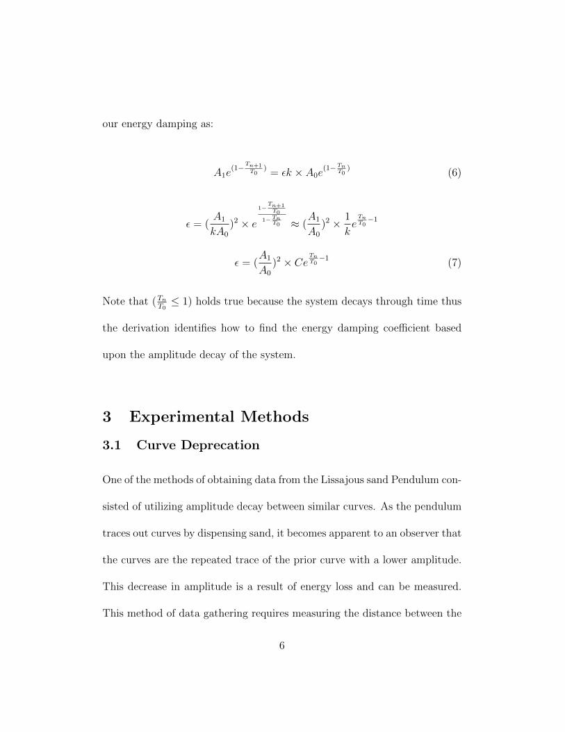
3.3 Simulation Comparison

The verification method of this experiment is to utilize the results of the

physical sand pendulum and contrast them with the idealistic curve traces.

In order to create ideal curve traces, I developed a script in Python to produce

the curves. This method enhances the verification of the physical curve traces

by utilizing a variable energy damping coefficient that can be adjusted until

the simulated traces share curve amplitude deprecation ratios identical to the

physical experiment. Once these values are matched, the energy coefficient

parameter models the energy damping coefficient for that trace curve model.

Figure 3: Ideal Simulated Lissajous Curve

9

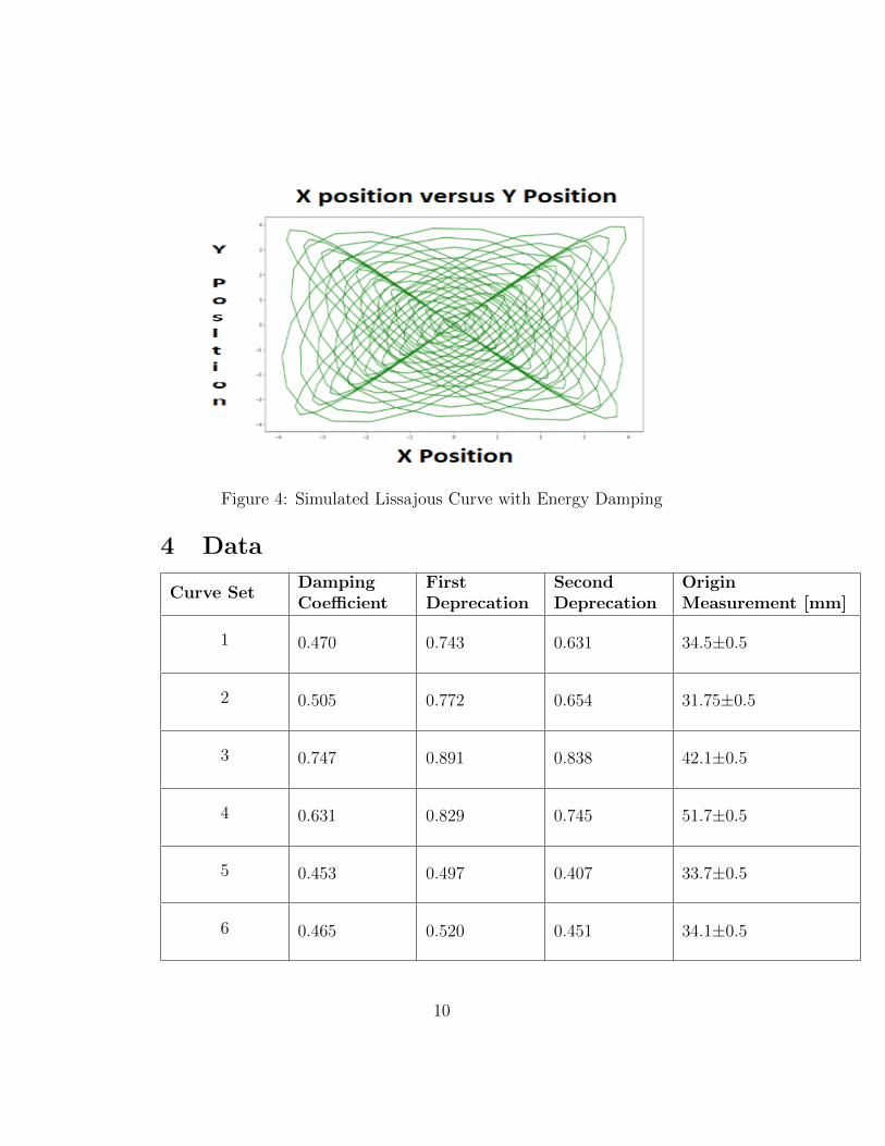
Figure 4: Simulated Lissajous Curve with Energy Damping

4 Data

Curve SetDampingCoefficient

FirstDeprecation

SecondDeprecation

OriginMeasurement [mm]

1 0.470 0.743 0.631 34.5±0.5

2 0.505 0.772 0.654 31.75±0.5

3 0.747 0.891 0.838 42.1±0.5

4 0.631 0.829 0.745 51.7±0.5

5 0.453 0.497 0.407 33.7±0.5

6 0.465 0.520 0.451 34.1±0.5

10

Figure 5: Graphical representation of curve set #1 total energy loss perperiod.

11

Figure 6: Graphical representation of curve set #2 total energy loss perperiod.

12

Figure 7: Graphical representation of curve set #3 total energy loss perperiod.

13

Figure 8: Graphical representation of curve set #4 total energy loss perperiod.

14

Figure 9: Graphical representation of curve set #5 total energy loss perperiod.

15

Figure 10: Graphical representation of curve set #6 total energy loss perperiod.

16

5 Conclusions

Preliminary data indicated that energy loss decays exponential within each

curve set. After further analysis, the relationship between curve set decay

became linear as periods shortened and longer periods tended towards expo-

nential decay. In addition to this observation, the identified trend classified

larger trace patterns as exhibiting longer initial periods of motion and con-

sequently exhibiting the largest energy damping effects. While discrepancies

in data existed, error-ridden data was corrected for by implementing the

origin-line tracing method.

Further experiments that could utilize or enhance these findings consists

of- using pendulum’s with different flow rates, measuring curve sets with

different height intervals, or swapping the sand pendulum out for LED’s and

perform a light tracing experiment of a Lissajous pendulum. All of the above

suggestions are different methods that can reveal new aspects of Lissajous

curves.

17

6 Bibliography

• The Motion of the Spherical Pendulum Subjected to a Dn SymmetricPerturbation. Pascal Chossat Nawaf M. Bou-Rabee

• The Moving Center of Mass of a Leaking Bob. P. Arun

7 Appendix

Figure 11: Full Pendulum with dimensions and knot description

18

Figure 12: Curve Set 1

Figure 13: Curve Set 2

19

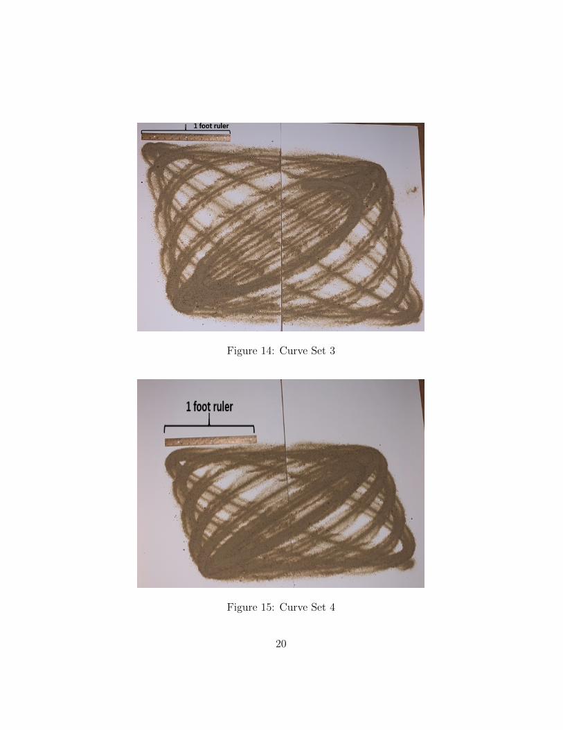
Figure 14: Curve Set 3

Figure 15: Curve Set 4

20

Figure 16: Curve Set 5

Figure 17: Curve Set 6

21