lissajous points for polynomial interpolation on …demarchi/taa1718/lissajous_presenta...lissajous...
TRANSCRIPT
Lissajous points for polynomial interpolation onvarious domains
Chiara Faccio
Dipartimento di Matematica "Tullio Levi-Civita"Università degli Studi di Padova
November 21, 2017
Chiara Faccio Lissajous points for polynomial interpolation on various domains

Contents
Definition of Lissajous curves
The node points of degenerate Lissajous curvesThe node points of non-degenerate Lissajous curvesInterpolation at the degenerate Lissajous pointsNumerical simulationsMorrow-Patterson, Padua and Xu points
Chiara Faccio Lissajous points for polynomial interpolation on various domains

Contents
Definition of Lissajous curvesThe node points of degenerate Lissajous curves
The node points of non-degenerate Lissajous curvesInterpolation at the degenerate Lissajous pointsNumerical simulationsMorrow-Patterson, Padua and Xu points
Chiara Faccio Lissajous points for polynomial interpolation on various domains

Contents
Definition of Lissajous curvesThe node points of degenerate Lissajous curvesThe node points of non-degenerate Lissajous curves
Interpolation at the degenerate Lissajous pointsNumerical simulationsMorrow-Patterson, Padua and Xu points
Chiara Faccio Lissajous points for polynomial interpolation on various domains

Contents
Definition of Lissajous curvesThe node points of degenerate Lissajous curvesThe node points of non-degenerate Lissajous curvesInterpolation at the degenerate Lissajous points
Numerical simulationsMorrow-Patterson, Padua and Xu points
Chiara Faccio Lissajous points for polynomial interpolation on various domains
Contents
Definition of Lissajous curvesThe node points of degenerate Lissajous curvesThe node points of non-degenerate Lissajous curvesInterpolation at the degenerate Lissajous pointsNumerical simulations
Morrow-Patterson, Padua and Xu points
Chiara Faccio Lissajous points for polynomial interpolation on various domains

Contents
Definition of Lissajous curvesThe node points of degenerate Lissajous curvesThe node points of non-degenerate Lissajous curvesInterpolation at the degenerate Lissajous pointsNumerical simulationsMorrow-Patterson, Padua and Xu points
Chiara Faccio Lissajous points for polynomial interpolation on various domains

Lissajous curves
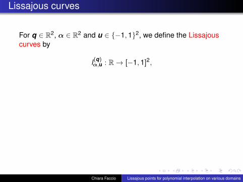
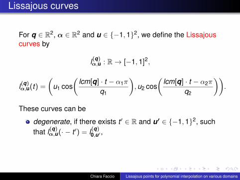
For q ∈ R2, α ∈ R2 and u ∈ {−1,1}2, we define the Lissajouscurves by
l(q)α,u : R→ [−1,1]2,
l(q)α,u(t) =
Çu1 cos
Çlcm[q] · t − α1π
q1
å,u2 cos
Çlcm[q] · t − α2π
q2
åå.
These curves can be
degenerate, if there exists t ′ ∈ R and u′ ∈ {−1,1}2, suchthat l(q)
α,u(· − t ′) = l(q)0,u′ ,
non − degenerate, otherwise.
Chiara Faccio Lissajous points for polynomial interpolation on various domains
Lissajous curves
For q ∈ R2, α ∈ R2 and u ∈ {−1,1}2, we define the Lissajouscurves by
l(q)α,u : R→ [−1,1]2,
l(q)α,u(t) =
Çu1 cos
Çlcm[q] · t − α1π
q1
å,u2 cos
Çlcm[q] · t − α2π
q2
åå.
These curves can be
degenerate, if there exists t ′ ∈ R and u′ ∈ {−1,1}2, suchthat l(q)
α,u(· − t ′) = l(q)0,u′ ,
non − degenerate, otherwise.
Chiara Faccio Lissajous points for polynomial interpolation on various domains

The Lissajous curve is a periodic function with period 2π.
If the Lissajous curve is degenerate, it is doubly traversed,so we can restrict the parametrization to [0, π].The pointsl(q)0,u (0) and l(q)
0,u (π) denote the starting and the end point ofthe curve;If the Lissajous curve is non − degenerate, we can find, upto finitely many exceptions, only one value of t ∈ [0,2π)corresponding to a point on the curve.
Chiara Faccio Lissajous points for polynomial interpolation on various domains

The Lissajous curve is a periodic function with period 2π.
If the Lissajous curve is degenerate, it is doubly traversed,so we can restrict the parametrization to [0, π].The pointsl(q)0,u (0) and l(q)
0,u (π) denote the starting and the end point ofthe curve;
If the Lissajous curve is non − degenerate, we can find, upto finitely many exceptions, only one value of t ∈ [0,2π)corresponding to a point on the curve.
Chiara Faccio Lissajous points for polynomial interpolation on various domains

The Lissajous curve is a periodic function with period 2π.
If the Lissajous curve is degenerate, it is doubly traversed,so we can restrict the parametrization to [0, π].The pointsl(q)0,u (0) and l(q)
0,u (π) denote the starting and the end point ofthe curve;If the Lissajous curve is non − degenerate, we can find, upto finitely many exceptions, only one value of t ∈ [0,2π)corresponding to a point on the curve.
Chiara Faccio Lissajous points for polynomial interpolation on various domains

Degenerate Lissajous curves
Consider the Lissajous figures of the type:
γn,p : [0, π]→ [−1,1]2
γn,p =
Çcos(nt), cos((n + p)t)
å= l(n+p,n)
0,1 (t)
with n and p positive integers such that n and n + p arerelatively prime.If we sample the curve along n(n + p) + 1 equidistant points
tk =πk
n(n + p), k = 0, ...,n(n + p)
in the interval [0, π], we get the Lissajous points
LDn,p := {γn,p(tk ) : k = 0, ...,n(n + p)}.
Chiara Faccio Lissajous points for polynomial interpolation on various domains

Degenerate Lissajous curves
Consider the Lissajous figures of the type:
γn,p : [0, π]→ [−1,1]2
γn,p =
Çcos(nt), cos((n + p)t)
å= l(n+p,n)
0,1 (t)
with n and p positive integers such that n and n + p arerelatively prime.
If we sample the curve along n(n + p) + 1 equidistant points
tk =πk
n(n + p), k = 0, ...,n(n + p)
in the interval [0, π], we get the Lissajous points
LDn,p := {γn,p(tk ) : k = 0, ...,n(n + p)}.
Chiara Faccio Lissajous points for polynomial interpolation on various domains

Degenerate Lissajous curves
Consider the Lissajous figures of the type:
γn,p : [0, π]→ [−1,1]2
γn,p =
Çcos(nt), cos((n + p)t)
å= l(n+p,n)
0,1 (t)
with n and p positive integers such that n and n + p arerelatively prime.If we sample the curve along n(n + p) + 1 equidistant points
tk =πk
n(n + p), k = 0, ...,n(n + p)
in the interval [0, π], we get the Lissajous points
LDn,p := {γn,p(tk ) : k = 0, ...,n(n + p)}.
Chiara Faccio Lissajous points for polynomial interpolation on various domains

This points are the self-intersections and boundarycontacts of the generating curve in [−1,1]2.
|LDn,p| = (n+p+1)(n+1)2
Figure: Lissajous curve γ4,3 and LD4,3.
Chiara Faccio Lissajous points for polynomial interpolation on various domains

This points are the self-intersections and boundarycontacts of the generating curve in [−1,1]2.
|LDn,p| = (n+p+1)(n+1)2
Figure: Lissajous curve γ4,3 and LD4,3.
Chiara Faccio Lissajous points for polynomial interpolation on various domains

This points are the self-intersections and boundarycontacts of the generating curve in [−1,1]2.
|LDn,p| = (n+p+1)(n+1)2
Figure: Lissajous curve γ4,3 and LD4,3.
Chiara Faccio Lissajous points for polynomial interpolation on various domains

We can describe the Lissajous curves and points in anotherway: we consider the algebraic Chebyshev variety
Cn,p := {(x , y) ∈ [−1,1]2 : Tn+p(x) = Tn(y)}
where Tn(x) = cos(narcos(x)) denotes the Chebyshevpolynomial of the first kind.
This algebraic variety corresponds to the degenerate Lissajouscurve and the singular points of Cn,p to the Lissajous points.
Chiara Faccio Lissajous points for polynomial interpolation on various domains

We can describe the Lissajous curves and points in anotherway: we consider the algebraic Chebyshev variety
Cn,p := {(x , y) ∈ [−1,1]2 : Tn+p(x) = Tn(y)}
where Tn(x) = cos(narcos(x)) denotes the Chebyshevpolynomial of the first kind.This algebraic variety corresponds to the degenerate Lissajouscurve and the singular points of Cn,p to the Lissajous points.
Chiara Faccio Lissajous points for polynomial interpolation on various domains

If we use the notation
znk := cos
Äkπn
ä, n ∈ N, k = 0, ...n
to abbreviate the Chebyshev-Lobatto points, we can describethe Lissajous points as
LDn,p = {(zn+pi , zn
j ) : i = 0, ...,n+p, j = 0, ...,n, i+j ≡ 0 mod2}
Example: for d = 1 and n ∈ N, we obtain ln0,1(t) = cos(t),ln0,1([0, π]) = [−1,1] and the points LDn = {zn
i : i = 0, ...,n} arethe univariate Chebyshev-Lobatto points.
Chiara Faccio Lissajous points for polynomial interpolation on various domains
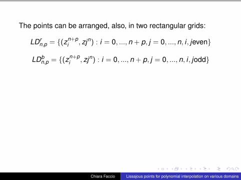
The points can be arranged, also, in two rectangular grids:
LDrn,p = {(zn+p
i , zjn) : i = 0, ...,n + p, j = 0, ...,n, i , jeven}
LDbn,p = {(zn+p
i , zjn) : i = 0, ...,n + p, j = 0, ...,n, i , jodd}
Introducing the index sets
ΓLn,p =
¶(i , j) ∈ N2
0 :i
n + p+
jn< 1©∪{(0,n)},
the note set LDn,p can be characterized as
LDn,p = {(zn+pin+j(n+p), z
nin+j(n+p)) : (i , j) ∈ ΓL
n,p)}.
Chiara Faccio Lissajous points for polynomial interpolation on various domains

Figure: Lissajous curve γ4,3 and LD4,3.
Chiara Faccio Lissajous points for polynomial interpolation on various domains

Non-degenerate Lissajous curves
We can consider the non-degenerate Lissajous curves of theform
λn,p = (sin(nt), sin((n + p)t)) = l2(n+p,n)(n+p,n),1(t)
where n and p are relatively prime. The curve isnon-degenerate if and only if p is odd.In this case, λn,p : [0,2π)→ R2 is sampled along the 4n(n + p)equidistant points
tk :=2πk
4n(n + p), k = 1, ...,4n(n + p).
In this way we get the following set of Lissajous node points:
LNDn,p := {λn,p(tk ) : k = 1, ...,4n(n + p)}.
Chiara Faccio Lissajous points for polynomial interpolation on various domains

Non-degenerate Lissajous curves
We can consider the non-degenerate Lissajous curves of theform
λn,p = (sin(nt), sin((n + p)t)) = l2(n+p,n)(n+p,n),1(t)
where n and p are relatively prime. The curve isnon-degenerate if and only if p is odd.
In this case, λn,p : [0,2π)→ R2 is sampled along the 4n(n + p)equidistant points
tk :=2πk
4n(n + p), k = 1, ...,4n(n + p).
In this way we get the following set of Lissajous node points:
LNDn,p := {λn,p(tk ) : k = 1, ...,4n(n + p)}.
Chiara Faccio Lissajous points for polynomial interpolation on various domains

Non-degenerate Lissajous curves
We can consider the non-degenerate Lissajous curves of theform
λn,p = (sin(nt), sin((n + p)t)) = l2(n+p,n)(n+p,n),1(t)
where n and p are relatively prime. The curve isnon-degenerate if and only if p is odd.In this case, λn,p : [0,2π)→ R2 is sampled along the 4n(n + p)equidistant points
tk :=2πk
4n(n + p), k = 1, ...,4n(n + p).
In this way we get the following set of Lissajous node points:
LNDn,p := {λn,p(tk ) : k = 1, ...,4n(n + p)}.
Chiara Faccio Lissajous points for polynomial interpolation on various domains

The non-degenerate Lissajous points are theself-intersections and boundary contacts of the Lissajouscurve in the square [−1,1]2;|LNDn,p| = 2n(n + p) + 2n + p;We can describe the points using the Chebyschev-Lobattopoints;The algebraic Chebyshev variety in this case is
Cn,p = {(x , y) ∈ [−1,1]2 : (−1)n+pT2n+2p(x) = (−1)nT2n(y)}.
The points can be arranged in two rectangular grids.
Chiara Faccio Lissajous points for polynomial interpolation on various domains

Figure: Lissajous curves λ2,1, |LND2,1| = 17 (left) and λ2,3,|LND2,3| = 27 (right).
Chiara Faccio Lissajous points for polynomial interpolation on various domains

Particular set of Lissajous points LC(2n)k
Now we consider this set of Lissajous points:
LC(10,6)0 = LC(10,6)
0,0 ∪ LC(10,6)0,1
LC2n0,τ = {(z(2n1)
i , z(2n2)j ) : (i , j) ∈ I(2n)
0,τ }
I(2n)0,τ = {(i , j) ∈ N0 :0 ≤ i ≤ 2n1 i ≡ τmod2,
0 ≤ j ≤ 2n2 j ≡ τmod2}
Chiara Faccio Lissajous points for polynomial interpolation on various domains

We notice that the sets LC(2n)0 are invariant under reflections
with the x and y axis, so we have the following characterizationof these Lisssajous points:
a point in LC(2n)k is a
self-intersection point of exactly one curve OR it is anintersection point of 2 curves.Now, we return to the inititial general notation:
l(2n)k ,u (t) = (u1 cos(2n1t − k1),u2 cos(2n2t − k2)).
The affine Chebyshev variety can be written as:
C(2n)k =
⋃u∈{−1,1}2
l(2n)k ,u ([0, π)).
Similar as for the degenerate curves, a point is a singular pointof C(2n)
k if and only if it is a Lissajous point.
Chiara Faccio Lissajous points for polynomial interpolation on various domains

We notice that the sets LC(2n)0 are invariant under reflections
with the x and y axis, so we have the following characterizationof these Lisssajous points: a point in LC(2n)
k is aself-intersection point of exactly one curve OR it is anintersection point of 2 curves.
Now, we return to the inititial general notation:
l(2n)k ,u (t) = (u1 cos(2n1t − k1),u2 cos(2n2t − k2)).
The affine Chebyshev variety can be written as:
C(2n)k =
⋃u∈{−1,1}2
l(2n)k ,u ([0, π)).
Similar as for the degenerate curves, a point is a singular pointof C(2n)
k if and only if it is a Lissajous point.
Chiara Faccio Lissajous points for polynomial interpolation on various domains
We notice that the sets LC(2n)0 are invariant under reflections
with the x and y axis, so we have the following characterizationof these Lisssajous points: a point in LC(2n)
k is aself-intersection point of exactly one curve OR it is anintersection point of 2 curves.Now, we return to the inititial general notation:
l(2n)k ,u (t) = (u1 cos(2n1t − k1),u2 cos(2n2t − k2)).
The affine Chebyshev variety can be written as:
C(2n)k =
⋃u∈{−1,1}2
l(2n)k ,u ([0, π)).
Similar as for the degenerate curves, a point is a singular pointof C(2n)
k if and only if it is a Lissajous point.
Chiara Faccio Lissajous points for polynomial interpolation on various domains

Figure: Lissajous curve l(10,6)0,(1,1)([0, π]) and LC(10,6)
0 .
Chiara Faccio Lissajous points for polynomial interpolation on various domains
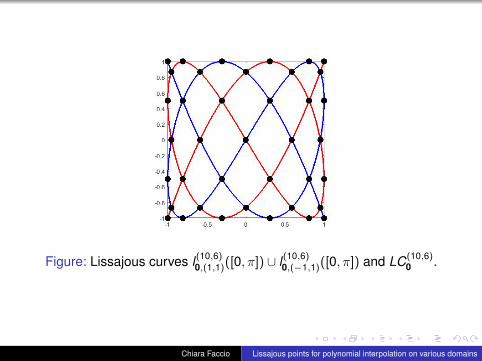
Figure: Lissajous curves l(10,6)0,(1,1)([0, π]) ∪ l(10,6)
0,(−1,1)([0, π]) and LC(10,6)0 .
Chiara Faccio Lissajous points for polynomial interpolation on various domains

Figure: Lissajous points LC2(5,2)(5,0) .
Chiara Faccio Lissajous points for polynomial interpolation on various domains

Unified theory for Lissajous points and curves
We make use of a decomposition of the parameter vector n:there exist integer vectors n∗,no ∈ N2 such that ∀i = 1,2:
ni = n∗i noi ;
n∗i and noi are relatively prime;
n∗1 and n∗2 are relatively prime;lcm[n] = n∗1n∗2.
We introduce the following sets :
R(no) = {0,1, ...,mo1 − 1} × {0,1, ...,mo
2 − 1}
I(n)k ,τ = {(i , j) ∈ N0 :0 ≤ i ≤ 2n1 i ≡ τmod2,
0 ≤ j ≤ 2n2 j ≡ τmod2}
Chiara Faccio Lissajous points for polynomial interpolation on various domains

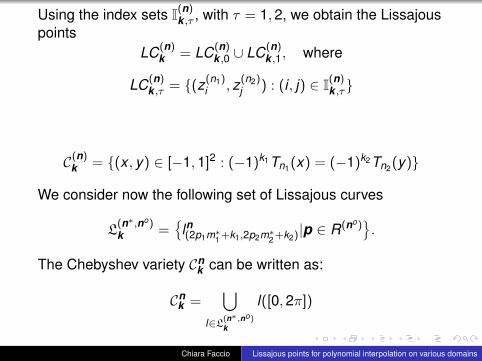
Using the index sets I(n)k ,τ , with τ = 1,2, we obtain the Lissajous
pointsLC(n)
k = LC(n)k ,0 ∪ LC(n)
k ,1, where
LC(n)k ,τ = {(z(n1)
i , z(n2)j ) : (i , j) ∈ I(n)
k ,τ}
C(n)k = {(x , y) ∈ [−1,1]2 : (−1)k1Tn1(x) = (−1)k2Tn2(y)}
We consider now the following set of Lissajous curves
L(n∗,no)k =
¶ln(2p1m∗1 +k1,2p2m∗2 +k2)|p ∈ R(no)
©.
The Chebyshev variety Cnk can be written as:
Cnk =
⋃l∈L(n∗,no)
k
l([0,2π])
Chiara Faccio Lissajous points for polynomial interpolation on various domains

The cardinality of L(n∗,no)k is #L
(n∗,no)k = 1
2(no1no
2 + Ndeg), wherethe number of degenerate curves Ndeg is
Ndeg =
1 if M0 = ∅,2#(K0∩M0)−1 if K0 ∩M0 6= ∅ and K1 ∩M0 = ∅2#(K1∩M0)−1 if K0 ∩M0 = ∅ and K1 ∩M0 6= ∅0 if K0 ∩M0 6= ∅ and K1 ∩M0 6= ∅
where for τ ∈ {(0,1} we denote
M0 = {i ∈ {1,2}|ni ≡ 0 mod2}
Kτ = {i ∈ {1,2}|ki ≡ τ mod2}.
Chiara Faccio Lissajous points for polynomial interpolation on various domains

Example: we consider the bivariate node set LC(10,5)(0,0) . We
have:
n = (10,5) k = (0,0),n∗ = (10,1) no = (1,5),
L(n∗,no)k = {ln(0,2p)|p ∈ {0,1,2}},
Cnk =
⋃p∈{0,2,4} l(10,5)
(0,p) ([0,2π]),
M0 = {1}, K0 = {1,2} K1 = ∅,Ndeg = 2#(K0∩M0)−1 = 20 = 1.
Chiara Faccio Lissajous points for polynomial interpolation on various domains

Figure: l(10,5)(0,0) ([0,2π))
Chiara Faccio Lissajous points for polynomial interpolation on various domains
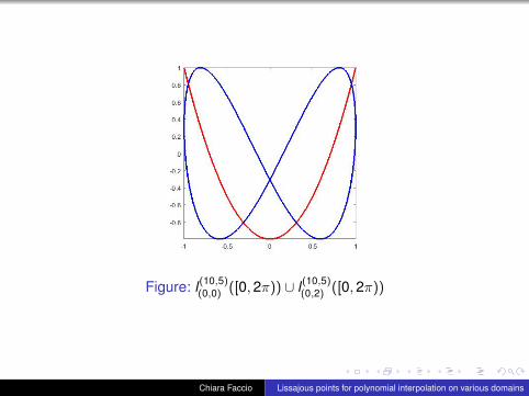
Figure: l(10,5)(0,0) ([0,2π)) ∪ l(10,5)
(0,2) ([0,2π))
Chiara Faccio Lissajous points for polynomial interpolation on various domains
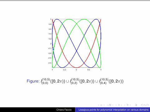
Figure: l(10,5)(0,0) ([0,2π)) ∪ l(10,5)
(0,2) ([0,2π)) ∪ l(10,5)(0,4) ([0,2π))
Chiara Faccio Lissajous points for polynomial interpolation on various domains

Figure: l(10,5)(0,0) ([0,2π)) ∪ l(10,5)
(0,2) ([0,2π)) ∪ l(10,5)(0,4) ([0,2π)) and LC(10,5)
(0,0)
Chiara Faccio Lissajous points for polynomial interpolation on various domains
Interpolation at the degenerate Lissajous points
Given data values f (A) ∈ R at the node points A ∈ LDn,p, theaim is to find the unique bivariate interpolating polynomial Ln,pfsuch that
Ln,pf (A) = f (A), ∀A ∈ LDn,p
Which polynomial space has to be chosen for the interpolationproblem?We introduce the space Π2,L
n,p = span{T̂i(x)T̂j(y) : (i , j) ∈ ΓLn,p},
where T̂i(x) is the normalized classical Chebyshev polynomialof the first kind of degree i ,
T̂i(x) =
{1, if i = 0,√
2Ti(x) if i 6= 0.
ΓLn,p =
¶(i , j) ∈ N2
0 :i
n + p+
jn< 1©∪{(0,n)},
Chiara Faccio Lissajous points for polynomial interpolation on various domains

Interpolation at the degenerate Lissajous points
Given data values f (A) ∈ R at the node points A ∈ LDn,p, theaim is to find the unique bivariate interpolating polynomial Ln,pfsuch that
Ln,pf (A) = f (A), ∀A ∈ LDn,p
Which polynomial space has to be chosen for the interpolationproblem?
We introduce the space Π2,Ln,p = span{T̂i(x)T̂j(y) : (i , j) ∈ ΓL
n,p},where T̂i(x) is the normalized classical Chebyshev polynomialof the first kind of degree i ,
T̂i(x) =
{1, if i = 0,√
2Ti(x) if i 6= 0.
ΓLn,p =
¶(i , j) ∈ N2
0 :i
n + p+
jn< 1©∪{(0,n)},
Chiara Faccio Lissajous points for polynomial interpolation on various domains

Interpolation at the degenerate Lissajous points
Given data values f (A) ∈ R at the node points A ∈ LDn,p, theaim is to find the unique bivariate interpolating polynomial Ln,pfsuch that
Ln,pf (A) = f (A), ∀A ∈ LDn,p
Which polynomial space has to be chosen for the interpolationproblem?We introduce the space Π2,L
n,p = span{T̂i(x)T̂j(y) : (i , j) ∈ ΓLn,p},
where T̂i(x) is the normalized classical Chebyshev polynomialof the first kind of degree i ,
T̂i(x) =
{1, if i = 0,√
2Ti(x) if i 6= 0.
ΓLn,p =
¶(i , j) ∈ N2
0 :i
n + p+
jn< 1©∪{(0,n)},
Chiara Faccio Lissajous points for polynomial interpolation on various domains

{T̂i(x)T̂j(y) : (i , j) ∈ ΓLn,p} forms an orthonormal basis for the
space Π2,Ln,p with respect to the inner product
〈f ,g〉 :=1π2
∫ 1
−1
∫ 1
−1f (x , y)g(x , y)
1√1− x2
1»1− y2
dx dy .
Since dim(Π2,Ln,p) = |ΓL
n,p| = |LDn,p|, our primary choice is thepolynomial space Π2,L
n,p.The space ((Π2,L
n,p, 〈·, ·〉) has the reproducing kernel
K Ln,p(A,B) =
∑(i,j)∈ΓL
n,p
T̂i(xA)T̂i(yA)T̂j(xB)T̂j(yB)
Chiara Faccio Lissajous points for polynomial interpolation on various domains

{T̂i(x)T̂j(y) : (i , j) ∈ ΓLn,p} forms an orthonormal basis for the
space Π2,Ln,p with respect to the inner product
〈f ,g〉 :=1π2
∫ 1
−1
∫ 1
−1f (x , y)g(x , y)
1√1− x2
1»1− y2
dx dy .
Since dim(Π2,Ln,p) = |ΓL
n,p| = |LDn,p|, our primary choice is thepolynomial space Π2,L
n,p.
The space ((Π2,Ln,p, 〈·, ·〉) has the reproducing kernel
K Ln,p(A,B) =
∑(i,j)∈ΓL
n,p
T̂i(xA)T̂i(yA)T̂j(xB)T̂j(yB)
Chiara Faccio Lissajous points for polynomial interpolation on various domains

{T̂i(x)T̂j(y) : (i , j) ∈ ΓLn,p} forms an orthonormal basis for the
space Π2,Ln,p with respect to the inner product
〈f ,g〉 :=1π2
∫ 1
−1
∫ 1
−1f (x , y)g(x , y)
1√1− x2
1»1− y2
dx dy .
Since dim(Π2,Ln,p) = |ΓL
n,p| = |LDn,p|, our primary choice is thepolynomial space Π2,L
n,p.The space ((Π2,L
n,p, 〈·, ·〉) has the reproducing kernel
K Ln,p(A,B) =
∑(i,j)∈ΓL
n,p
T̂i(xA)T̂i(yA)T̂j(xB)T̂j(yB)
Chiara Faccio Lissajous points for polynomial interpolation on various domains
The fundamental Lagrange polynomials of the Lissajous pointsare
LA(x , y) := ωA[K Ln,p((x , y);A)− 1
2T̂n(y)T̂n(yA)],
where
ωA :=1
n(n + p)
1/2, if A ∈ LDn,p is a vertex point,1, if A ∈ LDn,p is an edge point,2 if A ∈ LDn,p is an interior point,
Now, the interpolation problem has a unique solution in Π2,Ln,p
given by
Ln,pf (x , y) =∑
A∈LDn,p
LA(x , y)f (A)
Chiara Faccio Lissajous points for polynomial interpolation on various domains

We can rewrite the interpolating polynomial Ln,pf (x , y) in termsof the orthonormal Chebyshev basis. In this way, we obtain therepresentation
Ln,pf (x , y) =∑
i,j∈ΓLn,p
ci,j T̂i(x)T̂j(y),
with the Fourier-Lagrange coefficients ci,j = 〈Ln,pf , T̂i(x)T̂j(y)〉given by
ci,j =
{∑A∈LDn,p f (A)ωAT̂i(xA)T̂j(yA), if (i , j) ∈ Γn,p,
12∑A∈LDn,p f (A)ωAT̂n(yA), if (i,j) = (0,n).
Chiara Faccio Lissajous points for polynomial interpolation on various domains
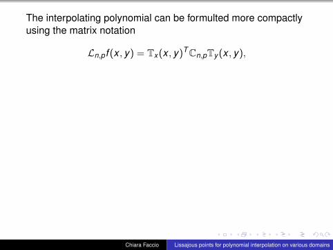
The interpolating polynomial can be formulted more compactlyusing the matrix notation
Ln,pf (x , y) = Tx (x , y)TCn,pTy (x , y),
whereCn,p = (Tx (LDn,p)Df (LDn,p)(Ty (LDn,p)T )�Mn,p,Df (LD,pn) = diag(ωAf (A),A ∈ LDn,p)
Tx (LDn,p) =
ÜT̂0(xA)
. . .... . . .
T̂n+p−1(xA)
êwith A ∈ LDn,p
Mn,p = (mi,j), mi,j =
1, if (i , j) ∈ Γn,p,1/2, if (i , j) = (0,n)
0. (i , j) /∈ ΓLn,p
Chiara Faccio Lissajous points for polynomial interpolation on various domains

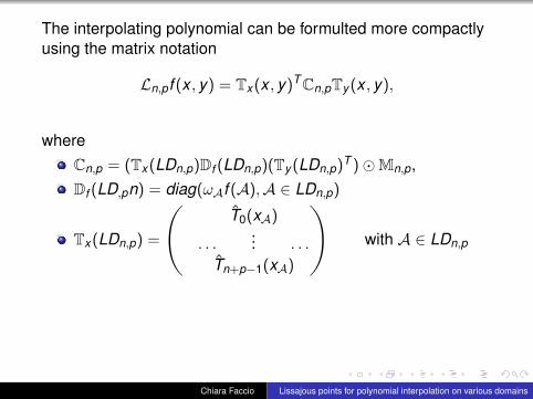
The interpolating polynomial can be formulted more compactlyusing the matrix notation
Ln,pf (x , y) = Tx (x , y)TCn,pTy (x , y),
whereCn,p = (Tx (LDn,p)Df (LDn,p)(Ty (LDn,p)T )�Mn,p,
Df (LD,pn) = diag(ωAf (A),A ∈ LDn,p)
Tx (LDn,p) =
ÜT̂0(xA)
. . .... . . .
T̂n+p−1(xA)
êwith A ∈ LDn,p
Mn,p = (mi,j), mi,j =
1, if (i , j) ∈ Γn,p,1/2, if (i , j) = (0,n)
0. (i , j) /∈ ΓLn,p
Chiara Faccio Lissajous points for polynomial interpolation on various domains

The interpolating polynomial can be formulted more compactlyusing the matrix notation
Ln,pf (x , y) = Tx (x , y)TCn,pTy (x , y),
whereCn,p = (Tx (LDn,p)Df (LDn,p)(Ty (LDn,p)T )�Mn,p,Df (LD,pn) = diag(ωAf (A),A ∈ LDn,p)
Tx (LDn,p) =
ÜT̂0(xA)
. . .... . . .
T̂n+p−1(xA)
êwith A ∈ LDn,p
Mn,p = (mi,j), mi,j =
1, if (i , j) ∈ Γn,p,1/2, if (i , j) = (0,n)
0. (i , j) /∈ ΓLn,p
Chiara Faccio Lissajous points for polynomial interpolation on various domains

The Lebesgue constant
The Lebesgue constant is the operator norm
Λn,p = maxf∈C([−1,1]2)
f 6=0
‖Ln,p(f )‖∞‖f‖∞
= max(x ,y)∈[−1,1]2
∑A∈LDn,p
|LA(x , y)|.
We investigate the Lebesgue constant Λn,pn for the parameterspn ∈ {1,n + 1}. The values are illustrated for 1 ≤ n ≤ 50. For abetter comparison we plot also the functions f1(n) and f2(n), asa lower and an upper benchmark:
f1(n) =Ä2π
log(n + 1) + 1ä2
f2(n) =Ä2π
log(n + 1) +32
ä2
Chiara Faccio Lissajous points for polynomial interpolation on various domains

The Lebesgue constant
The Lebesgue constant is the operator norm
Λn,p = maxf∈C([−1,1]2)
f 6=0
‖Ln,p(f )‖∞‖f‖∞
= max(x ,y)∈[−1,1]2
∑A∈LDn,p
|LA(x , y)|.
We investigate the Lebesgue constant Λn,pn for the parameterspn ∈ {1,n + 1}. The values are illustrated for 1 ≤ n ≤ 50. For abetter comparison we plot also the functions f1(n) and f2(n), asa lower and an upper benchmark:
f1(n) =Ä2π
log(n + 1) + 1ä2
f2(n) =Ä2π
log(n + 1) +32
ä2Chiara Faccio Lissajous points for polynomial interpolation on various domains

Figure: The Lebesgue constant for the parameters pn ∈ {1,n + 1}.
TheoremThe Lebesgue constant Λn,p is bounded
DΛ ln2(n) ≤ Λn,p ≤ CΛ ln2(n + p),
where the constants DΛ and CΛ are independent of n and p.
Chiara Faccio Lissajous points for polynomial interpolation on various domains

Figure: The Lebesgue constant for the parameters pn ∈ {1,n + 1}.
TheoremThe Lebesgue constant Λn,p is bounded
DΛ ln2(n) ≤ Λn,p ≤ CΛ ln2(n + p),
where the constants DΛ and CΛ are independent of n and p.
Chiara Faccio Lissajous points for polynomial interpolation on various domains
Numerical examples
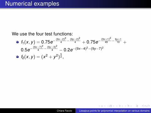
We use the four test functions:
f1(x , y) = 0.75e−(9x−2)2
4 − (9y−2)2
4 + 0.75e−(9x+1)2
49 − 9y+110 +
0.5e−(9x−7)2
4 − (9y−3)2
4 − 0.2e−(9x−4)2−(9y−7)2
f2(x , y) = (x2 + y2)52 ,
f3(x , y) = e−(5−10x)2
2 + 0.75e−(5−10y)2
2 + 0.75e−(5−10x)2+(5−10y)2
2
f4(x , y) = (x + y)20.
Chiara Faccio Lissajous points for polynomial interpolation on various domains
Numerical examples
We use the four test functions:
f1(x , y) = 0.75e−(9x−2)2
4 − (9y−2)2
4 + 0.75e−(9x+1)2
49 − 9y+110 +
0.5e−(9x−7)2
4 − (9y−3)2
4 − 0.2e−(9x−4)2−(9y−7)2
f2(x , y) = (x2 + y2)52 ,
f3(x , y) = e−(5−10x)2
2 + 0.75e−(5−10y)2
2 + 0.75e−(5−10x)2+(5−10y)2
2
f4(x , y) = (x + y)20.
Chiara Faccio Lissajous points for polynomial interpolation on various domains
‖Ln,pn (f )− f‖∞ on the domain [−1,1]2, for three differentparameters pn ∈ {1,n + 1,n2 + 1} and 2 ≤ n ≤ 50.The maximal error is computed on a uniform grid of 60× 60points defined in the square [−1,1]2.
Figure: Absolute errors for f1 (left) and f2 (right).
Chiara Faccio Lissajous points for polynomial interpolation on various domains

Figure: Absolute errors for f3 (left) and f4 (right).
Chiara Faccio Lissajous points for polynomial interpolation on various domains

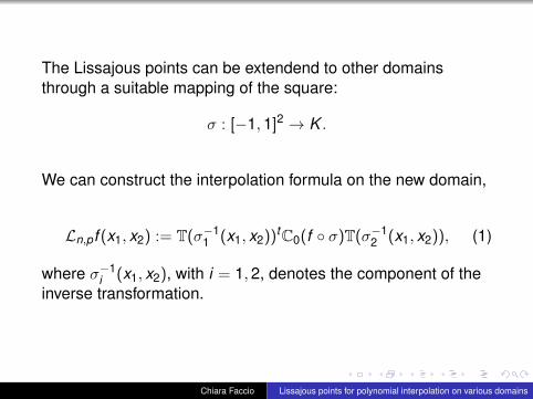
The Lissajous points can be extendend to other domainsthrough a suitable mapping of the square:
σ : [−1,1]2 → K .
We can construct the interpolation formula on the new domain,
Ln,pf (x1, x2) := T(σ−11 (x1, x2))tC0(f ◦ σ)T(σ−1
2 (x1, x2)), (1)
where σ−1i (x1, x2), with i = 1,2, denotes the component of the
inverse transformation.
Chiara Faccio Lissajous points for polynomial interpolation on various domains

Rectangle
σ(t1, t2) =
Çb − a
2t1 +
b + a2
,d − c
2t2 +
d + c2
å.
The inverse is given by
t1(x1, x2) = −1+2x1 − ab − a
, t2(x1, x2) =
{−1 + 2x2−c
d−c if c 6= d−1 if c = d
Figure: Absolute errors for f3 on [−1,1]2 (left) and on [0,2]× [0,1](right).
Chiara Faccio Lissajous points for polynomial interpolation on various domains

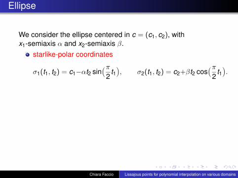
Ellipse
We consider the ellipse centered in c = (c1, c2), withx1-semiaxis α and x2-semiaxis β.
starlike-polar coordinates
σ1(t1, t2) = c1−αt2 sinÄπ
2t1ä, σ2(t1, t2) = c2+βt2 cos
Äπ2
t1ä.
standard polar coordinates
σ1(t1, t2) = ρ cos(θ), σ2(t1, t2) = ρ sin(θ)
θ(t1, t2) = π(t1+1), ρ(t1, t2) = (t2+1)r(θ)
2, r(θ) =
β2/α
1− ecos(θ).
Chiara Faccio Lissajous points for polynomial interpolation on various domains

Figure: The distribution of the Padua points and the Lissajous curvesin the ellipse with polar (left) and starlike-polar (right) for n = 33.
Chiara Faccio Lissajous points for polynomial interpolation on various domains

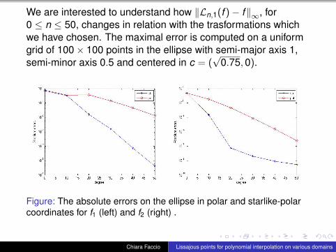
We are interested to understand how ‖Ln,1(f )− f‖∞, for0 ≤ n ≤ 50, changes in relation with the trasformations whichwe have chosen. The maximal error is computed on a uniformgrid of 100× 100 points in the ellipse with semi-major axis 1,semi-minor axis 0.5 and centered in c = (
√0.75,0).
Figure: The absolute errors on the ellipse in polar and starlike-polarcoordinates for f1 (left) and f2 (right) .
Chiara Faccio Lissajous points for polynomial interpolation on various domains

Diamond
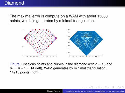
The maximal error is compute on a WAM with about 15000points, which is generated by minimal triangulation.
Figure: Lissajous points and curves in the diamond with n = 13 andpn = n + 1 = 14 (left), WAM generates by minimal triangulation,14913 points (right) .
Chiara Faccio Lissajous points for polynomial interpolation on various domains
Diamond
The maximal error is compute on a WAM with about 15000points, which is generated by minimal triangulation.
Figure: Lissajous points and curves in the diamond with n = 13 andpn = n + 1 = 14 (left), WAM generates by minimal triangulation,14913 points (right) .
Chiara Faccio Lissajous points for polynomial interpolation on various domains

Figure: Absolute errors for f2 (left) and f3 (right).
Chiara Faccio Lissajous points for polynomial interpolation on various domains

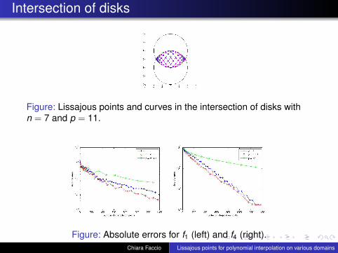
Intersection of disks
Figure: Lissajous points and curves in the intersection of disks withn = 7 and p = 11.
Figure: Absolute errors for f1 (left) and f4 (right).
Chiara Faccio Lissajous points for polynomial interpolation on various domains

Intersection of disks
Figure: Lissajous points and curves in the intersection of disks withn = 7 and p = 11.
Figure: Absolute errors for f1 (left) and f4 (right).
Chiara Faccio Lissajous points for polynomial interpolation on various domains
Intersection of disks
Figure: Lissajous points and curves in the intersection of disks withn = 7 and p = 11.
Figure: Absolute errors for f1 (left) and f4 (right).Chiara Faccio Lissajous points for polynomial interpolation on various domains

Star
Figure: Distribution of Padua points and curves with minimal andbarycentric triangulation. n = 5 (168 points left, 210 points right ).
Triangulation for f2 n = 2 n = 10 n = 20minimal triang. 7.98e + 01 3.81e − 03 9.85e − 05
barycentric triang. 7.87e + 01 9.90e − 07 1.68e − 10
Table: Absolute errors with different triangulations for f2.
Chiara Faccio Lissajous points for polynomial interpolation on various domains

To map, instead, the Lissajous points in the star we use theSchwarz-Christoffel functions. These are conformal maps fromthe unit disk onto various domains. In the case of our star themapping is
f (z) =
∫ z
0
(1− w5)2/5
(1 + w5)4/5 dw
Figure: Padua points in the star with n = 5, i.e. with 21 points (left)and n = 20 i.e. 231 points (right).
Chiara Faccio Lissajous points for polynomial interpolation on various domains
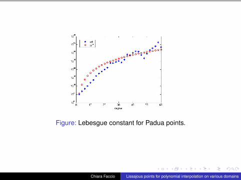
Figure: Lebesgue constant for Padua points.
Chiara Faccio Lissajous points for polynomial interpolation on various domains

Morrow-Patterson points
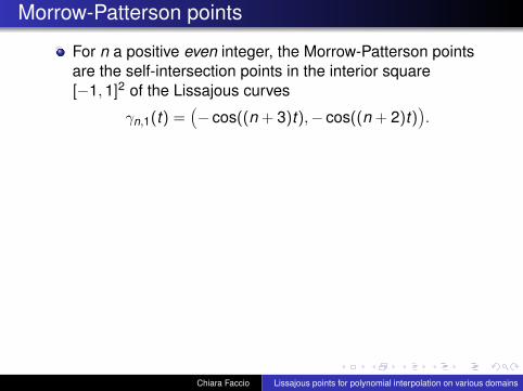
For n a positive even integer, the Morrow-Patterson pointsare the self-intersection points in the interior square[−1,1]2 of the Lissajous curves
γn,1(t) =Ä− cos((n + 3)t),− cos((n + 2)t)
ä.
|MPn| = dim(Π2n) =
(n+2n), and this set is unisolvent for
polynomial interpolation on the square [−1,1]2.
Figure: The curve γ6,1(t) and associated MP6.
Chiara Faccio Lissajous points for polynomial interpolation on various domains
Morrow-Patterson points
For n a positive even integer, the Morrow-Patterson pointsare the self-intersection points in the interior square[−1,1]2 of the Lissajous curves
γn,1(t) =Ä− cos((n + 3)t),− cos((n + 2)t)
ä.
|MPn| = dim(Π2n) =
(n+2n), and this set is unisolvent for
polynomial interpolation on the square [−1,1]2.
Figure: The curve γ6,1(t) and associated MP6.
Chiara Faccio Lissajous points for polynomial interpolation on various domains

Morrow-Patterson points
For n a positive even integer, the Morrow-Patterson pointsare the self-intersection points in the interior square[−1,1]2 of the Lissajous curves
γn,1(t) =Ä− cos((n + 3)t),− cos((n + 2)t)
ä.
|MPn| = dim(Π2n) =
(n+2n), and this set is unisolvent for
polynomial interpolation on the square [−1,1]2.
Figure: The curve γ6,1(t) and associated MP6.Chiara Faccio Lissajous points for polynomial interpolation on various domains

Padua points
They are the self-intersections and boundary contacts ofthe generating curve γn,1 = (− cos((n + 1)t),− cos(nt)) in[−1,1]2.They match exactly the dimension of Π2
n and they areunisolvent.They are modified Morrow-Patterson points.
Figure: MP6 and PD6 with respective Lissajous curves (left), MP6 andPD8 with respective Lissajous curves (right).
Chiara Faccio Lissajous points for polynomial interpolation on various domains

Padua points
They are the self-intersections and boundary contacts ofthe generating curve γn,1 = (− cos((n + 1)t),− cos(nt)) in[−1,1]2.
They match exactly the dimension of Π2n and they are
unisolvent.They are modified Morrow-Patterson points.
Figure: MP6 and PD6 with respective Lissajous curves (left), MP6 andPD8 with respective Lissajous curves (right).
Chiara Faccio Lissajous points for polynomial interpolation on various domains

Padua points
They are the self-intersections and boundary contacts ofthe generating curve γn,1 = (− cos((n + 1)t),− cos(nt)) in[−1,1]2.They match exactly the dimension of Π2
n and they areunisolvent.
They are modified Morrow-Patterson points.
Figure: MP6 and PD6 with respective Lissajous curves (left), MP6 andPD8 with respective Lissajous curves (right).
Chiara Faccio Lissajous points for polynomial interpolation on various domains

Padua points
They are the self-intersections and boundary contacts ofthe generating curve γn,1 = (− cos((n + 1)t),− cos(nt)) in[−1,1]2.They match exactly the dimension of Π2
n and they areunisolvent.They are modified Morrow-Patterson points.
Figure: MP6 and PD6 with respective Lissajous curves (left), MP6 andPD8 with respective Lissajous curves (right).
Chiara Faccio Lissajous points for polynomial interpolation on various domains

Padua points
They are the self-intersections and boundary contacts ofthe generating curve γn,1 = (− cos((n + 1)t),− cos(nt)) in[−1,1]2.They match exactly the dimension of Π2
n and they areunisolvent.They are modified Morrow-Patterson points.
Figure: MP6 and PD6 with respective Lissajous curves (left), MP6 andPD8 with respective Lissajous curves (right).
Chiara Faccio Lissajous points for polynomial interpolation on various domains

Xu points
They are Lissajous points, but their cardinality depends on thedegree;
if n is even, i.e. n = 2m, there are n(n+2)2 points,
LC(2m,2m)(0,1) =
(z2i , z2j+1), 0 ≤ i ≤ m,0 ≤ j ≤ m − 1,(z2i+1, z2j), 0 ≤ i ≤ m − 1,0 ≤ j ≤ m.
if n is odd, i.e. n = 2m + 1, there are (n+1)2
2 points,LC(2m+1,2m+1)
(0,0) =
(z2i , z2j), 0 ≤ i ≤ m,0 ≤ j ≤ m,(z2i+1, z2j+1), 0 ≤ i ≤ m,0 ≤ j ≤ m.
Chiara Faccio Lissajous points for polynomial interpolation on various domains
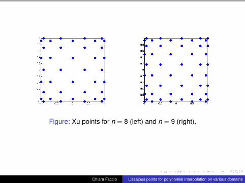
Figure: Xu points for n = 8 (left) and n = 9 (right).
Chiara Faccio Lissajous points for polynomial interpolation on various domains

n = (n,n),n∗ = (n,1),no = (1,n),
the curves in L(n∗,no)k are ellipses in [−1,1]2,
#L(n∗,no)k =
{n+1
2 if n is oddn2 if n is even
Ndeg =
{1 if n is odd0 if n is even
Chiara Faccio Lissajous points for polynomial interpolation on various domains

Figure: Xu points and curves for n = 4 (left) and n = 5 (right).
Chiara Faccio Lissajous points for polynomial interpolation on various domains

Figure: Interpolation errors for the function f2 .
Figure: The behaviour of the Lebesgue constant for Padua, Xu andMorrow-Patterson points.
Chiara Faccio Lissajous points for polynomial interpolation on various domains

Figure: Interpolation errors for the function f2 .
Figure: The behaviour of the Lebesgue constant for Padua, Xu andMorrow-Patterson points.
Chiara Faccio Lissajous points for polynomial interpolation on various domains

We compare the distribution of Padua, Xu and degenerateLissajous points.
Figure: PD5 (left), XU6 (middle) and LD5,2 (right) .
Chiara Faccio Lissajous points for polynomial interpolation on various domains

We compare the distribution of Padua, Xu and degenerateLissajous points.
Figure: PD5 (left), XU6 (middle) and LD5,2 (right) .
Chiara Faccio Lissajous points for polynomial interpolation on various domains

Thank you
Chiara Faccio Lissajous points for polynomial interpolation on various domains