modeling and simulation of air compressor energy...

ACEEE Summer Study on Energy in Industry, West Point, NY, July 19-22. 1

Modeling and Simulation of Air Compressor Energy Use

Chris Schmidt, Energy & Resource Solutions, Inc.

Kelly Kissock, Department of Mechanical Engineering, University of Dayton

ABSTRACT

This paper describes modeling and simulation of air compressor energy use to estimate energy savings in compressed air systems from air use reduction and other changes. The method uses measured power signatures and other compressor parameters as inputs to calculate various performance metrics and estimate energy savings. To enable recognition of control mode from measured power data, examples of power signatures for various control modes are shown. A generalized method for modeling the relationship between compressor power consumption and air output is developed. The use of this method to estimate energy savings from changing control modes and reducing air use is described and demonstrated with examples. Additional relationships for modeling compressor power as a function of system pressure, and for modeling the change in system pressure as function of compressed air storage volume are developed. The use of these relations in algorithms for modeling compressor control modes is described. The incorporation of these methods into new public-domain software for modeling air compressor energy use is described. Techniques for calibrating the software to measured energy use data, and estimating energy savings from retrofits are demonstrated with case study examples.

Introduction

Based on over 50 energy assessments of mid-sized industries, we found that the average unit energy cost of compressed air ranges from about $0.15 to $0.35 per thousand standard cubic feet and frequently comprises between 5% to 20% of a plant’s annual electric costs. The wide range in unit energy costs is a function of many factors, including cost of energy and number of compressors in operation. However, two of the most important factors influencing the cost of compressed air are the type of compressor control and proper compressor sizing. Oversized compressors, and compressors operating in inefficient control modes have the highest unit energy and annual operating costs.

In this paper, we describe common types of compressor control and how to recognize control type based on their power consumption signatures. Next, we present a method for calculating compressed air output based on the control type and measured compressor power data. The use of this method for estimating energy savings from reducing compressed air demand, reducing system pressure or changing control mode is described. A case study example demonstrates the importance of using this method to determine savings from reducing compressed air demand; failure to do so can lead to overestimation of savings by 500%.

In many cases, it is advantageous to incorporate these models into simulation software that can be quickly calibrated to measured energy use and system pressure. The paper describes the incorporation of these methods into a new public-domain software application for modeling air compressor energy use. An example of calibrating the simulation model to measured energy use and estimating savings from changing system parameters is demonstrated. The software can be used to estimate energy savings from reducing compressed air use, increasing system storage, changing the control mode, or modifying activation pressures.


Power Characteristics of Common Control Modes

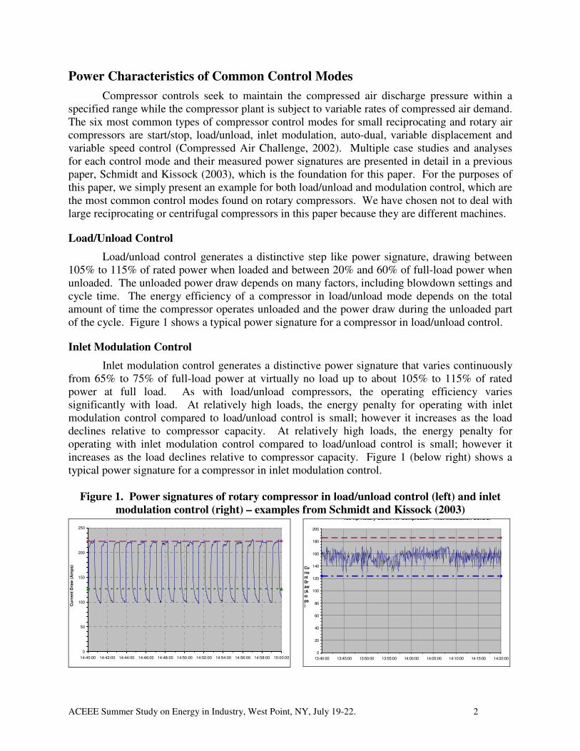
Compressor controls seek to maintain the compressed air discharge pressure within a specified range while the compressor plant is subject to variable rates of compressed air demand. The six most common types of compressor control modes for small reciprocating and rotary air compressors are start/stop, load/unload, inlet modulation, auto-dual, variable displacement and variable speed control (Compressed Air Challenge, 2002). Multiple case studies and analyses for each control mode and their measured power signatures are presented in detail in a previous paper, Schmidt and Kissock (2003), which is the foundation for this paper. For the purposes of this paper, we simply present an example for both load/unload and modulation control, which are the most common control modes found on rotary compressors. We have chosen not to deal with large reciprocating or centrifugal compressors in this paper because they are different machines.

Load/Unload Control

Load/unload control generates a distinctive step like power signature, drawing between 105% to 115% of rated power when loaded and between 20% and 60% of full-load power when unloaded. The unloaded power draw depends on many factors, including blowdown settings and cycle time. The energy efficiency of a compressor in load/unload mode depends on the total amount of time the compressor operates unloaded and the power draw during the unloaded part of the cycle. Figure 1 shows a typical power signature for a compressor in load/unload control.

Inlet Modulation Control

Inlet modulation control generates a distinctive power signature that varies continuously from 65% to 75% of full-load power at virtually no load up to about 105% to 115% of rated power at full load. As with load/unload compressors, the operating efficiency varies significantly with load. At relatively high loads, the energy penalty for operating with inlet modulation control compared to load/unload control is small; however it increases as the load declines relative to compressor capacity. At relatively high loads, the energy penalty for operating with inlet modulation control compared to load/unload control is small; however it increases as the load declines relative to compressor capacity. Figure 1 (below right) shows a typical power signature for a compressor in inlet modulation control.

Figure 1. Power signatures of rotary compressor in load/unload control (left) and inlet

modulation control (right) – examples from Schmidt and Kissock (2003)

0

50

100

150

200

250

14:40:00 14:42:00 14:44:00 14:46:00 14:48:00 14:50:00 14:52:00 14:54:00 14:56:00 14:58:00 15:00:00

Cu

rre

nt

Dra

w (

Am

ps

)

150-hp Rotary-Screw Air Compressor - Inlet Modulation Control

0 20 40 60 80

100 120 140 160 180 200

13:40:00 13:45:00 13:50:00 13:55:00 14:00:00 14:05:00 14:10:00 14:15:00 14:20:00

Current Draw (Amps)


Modeling the Relationship Between Air Compressor Power and Output

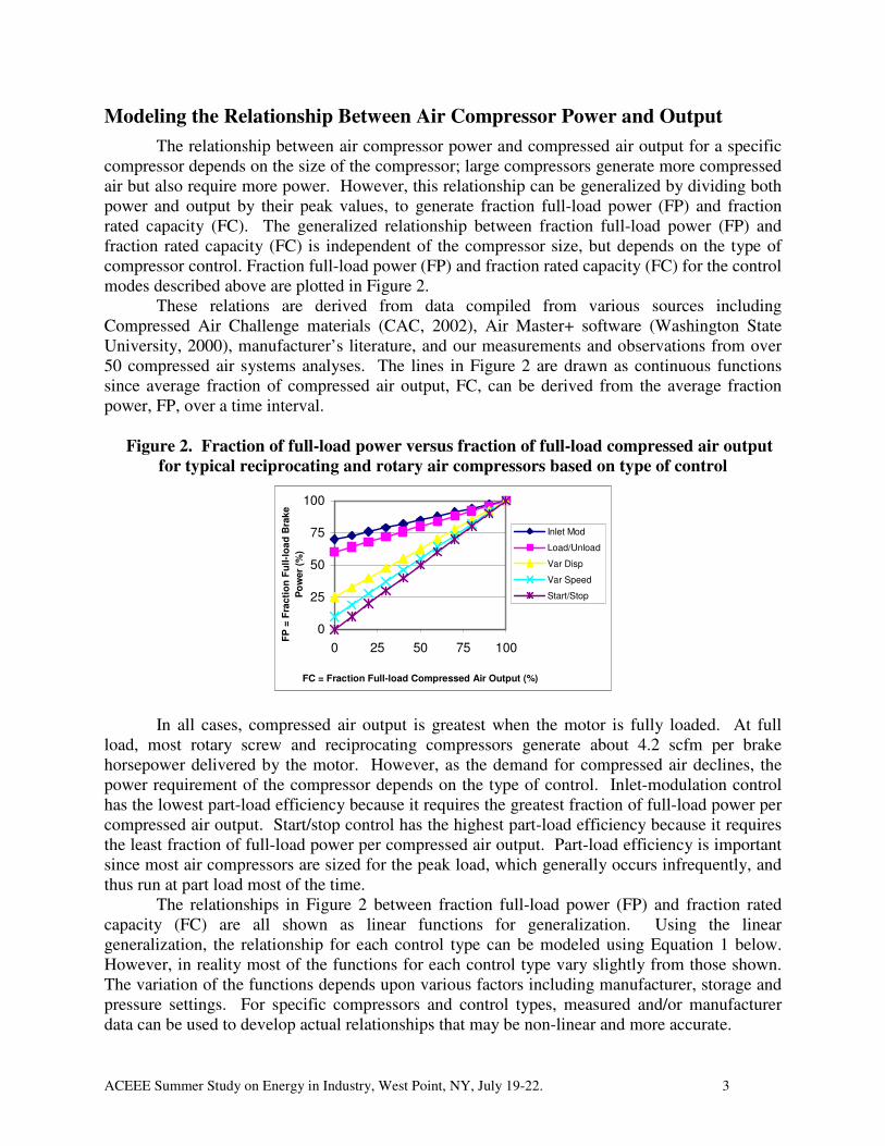
The relationship between air compressor power and compressed air output for a specific compressor depends on the size of the compressor; large compressors generate more compressed air but also require more power. However, this relationship can be generalized by dividing both power and output by their peak values, to generate fraction full-load power (FP) and fraction rated capacity (FC). The generalized relationship between fraction full-load power (FP) and fraction rated capacity (FC) is independent of the compressor size, but depends on the type of compressor control. Fraction full-load power (FP) and fraction rated capacity (FC) for the control modes described above are plotted in Figure 2.

These relations are derived from data compiled from various sources including Compressed Air Challenge materials (CAC, 2002), Air Master+ software (Washington State University, 2000), manufacturer’s literature, and our measurements and observations from over 50 compressed air systems analyses. The lines in Figure 2 are drawn as continuous functions since average fraction of compressed air output, FC, can be derived from the average fraction power, FP, over a time interval.

Figure 2. Fraction of full-load power versus fraction of full-load compressed air output

for typical reciprocating and rotary air compressors based on type of control

0

25

50

75

100

0 25 50 75 100

FC = Fraction Full-load Compressed Air Output (%)

FP

= F

racti

on

Fu

ll-l

oa

d B

rake

Po

wer

(%)

Inlet Mod

Load/Unload

Var Disp

Var Speed

Start/Stop

In all cases, compressed air output is greatest when the motor is fully loaded. At full load, most rotary screw and reciprocating compressors generate about 4.2 scfm per brake horsepower delivered by the motor. However, as the demand for compressed air declines, the power requirement of the compressor depends on the type of control. Inlet-modulation control has the lowest part-load efficiency because it requires the greatest fraction of full-load power per compressed air output. Start/stop control has the highest part-load efficiency because it requires the least fraction of full-load power per compressed air output. Part-load efficiency is important since most air compressors are sized for the peak load, which generally occurs infrequently, and thus run at part load most of the time.

The relationships in Figure 2 between fraction full-load power (FP) and fraction rated capacity (FC) are all shown as linear functions for generalization. Using the linear generalization, the relationship for each control type can be modeled using Equation 1 below. However, in reality most of the functions for each control type vary slightly from those shown. The variation of the functions depends upon various factors including manufacturer, storage and pressure settings. For specific compressors and control types, measured and/or manufacturer data can be used to develop actual relationships that may be non-linear and more accurate.


FP = FP0 + (1 – FP0) FC (1)

where FP0 is the fraction of full-load power when producing no compressed air. Graphically, FP0 is the y-intercept in Figure 2. The normalized power and capacity coefficients in Equation 1 are the actual power and capacity divided by the maximum power and capacity:

FP = P / FLP (2) FC = C / FLC (3) FP0 = P0 / FLP (4)

where P is the actual power and FLP is the full-load power; C is the actual output capacity and FLC is the full-load output capacity; and P0 is the power when producing no compressed air. In many cases, Equation 1 is solved to calculate average compressed air output, C, since the energy use of a compressor is more easily measured than the compressed air output. The values for a compressor’s power characteristics, P, P0 and FLP, can typically be determined from the measured power signatures, such as those shown in the previous section. If power at zero capacity, P0, cannot be determined from the power signature or from manufacturer data, it can be reasonably estimated using the y-intercept values shown in Figure 2 above. If full-load power, FLP, cannot be determined from the power signature or from manufacturer data, it can be reasonably estimated as 105% of the rated motor power. Finally, the full load output capacity of a compressor, FLC, can be obtained from the compressor nameplate or from manufacturer data. If not, it can be reasonably estimated for most rotary and reciprocating compressors as the product of the full-load power, FLP, and 4.2 scfm per horsepower.

Estimating Energy Savings in Compressed Air Systems

The following examples demonstrate the use of Equations 1- 4 to estimate energy savings. Additional examples are presented in Schmidt and Kissock (2004).

Operating in A More Efficient Control Mode

Many rotary compressors can be set to operate in either load/unload or modulation control. As presented above, the part-load efficiency of load/unload control is much better than modulation control and thus more energy efficient. Furthermore, most compressors with load/unload control also have auto shutoff capabilities. With auto shutoff, the compressor will automatically turn off if it runs unloaded for an adjustable time delay, and turn on again when the pressure reaches the load setting, reducing energy use during periods of low demand.

Unfortunately, we find many non-base loaded compressors set to operate in modulation control or with the auto-shutoff control deactivated. In this section, we show an example of quantifying expected savings from switching from modulation to load/unload control. The general method for calculating savings from changing control modes is to:

� Use measured power data and compressor specifications to determine P, P0 and FLP � Calculate FP and FP0 using Equations 2 and 4 � Calculate the current FC using Equation 1 � Calculate the expected FP using the FP0 for the improved control mode using Equation 1 � Calculate the expected P for the improved control mode using Equation 2 � Calculate energy savings as the difference between current and expected P.


A metal forming plant has a single 60-hp rotary compressor operating in modulation control. The average power draw of the compressor, P, was measured to be about 47 kW. Based on the rated full load amps from the compressor nameplate, the full-load power, FLP, was calculated to be 52 kW. The no-load power draw, P0, was determined to be 37 kW. From Equation 2, the fraction of full-load power FP is about:

FP = P / FLP = 47 kW / 52 kW = 90%

From Equation 4, the fraction of full-load power at no-load, FP0, is about:

FP0 = 37 kW / 52 kW = 71%

Substituting FP and FP0 into Equation 1, the average fraction of rated capacity, FC, is about:

FC = (0.90 - 0.71) / 0.19 = 65.5%

Based on previous measurements of this model compressor, the fraction of full-load power when unloaded, FP0, is about 55%. Thus, if the compressor were operated in load/unload mode at the same fraction of rated capacity, the expected FP from Equation 1 would be about:

FP2 = 0.55 + (1 – 0.55)*0.655 = 84.5%

From Equation 2, the expected average power would be about:

P2 = FP2 x FLP = 52 kW x 84.5% = 44 kW

The compressor operated for about 4,000 hours per year. Thus, the annual electricity savings from switching the compressor from modulation to load/unload control would be about:

47 kW – 44 kW = 3 kW 3 kW x 4,000 hr/yr = 12,000 kWh/yr

This example shows how operating compressors in load/unload mode can attain

significant savings.

Demand Side Reduction

The method demonstrated above to predict energy savings from switching to a more efficient control can also be used to predict savings from reducing compressed air demand. The general method for calculating savings from reducing compressed air demand is to:

� Use measured power data and compressor specs to determine P, P0, FLC and FLP � Calculate FP and FP0 using Equations 2 and 4. � Calculate the current FC using Equation 1 � Calculate the current C using Equation 3 � Calculate the expected C after compressed air demand is reduced � Calculate the expected FC at the reduced C using Equation 3 � Solve for the expected FP at the reduced FC using Equation 1 � Solve for the expected P at the reduced FP using Equation 2 � Calculate energy savings as the difference between current and expected P.


To illustrate the importance of the compressor control mode when calculating savings from reducing compressed air demand, consider a continuation of the previous example of the 60-hp compressor in modulation control. The rated full-load capacity, FLC, was 265 scfm. Thus, from Equation 3, the average output of the compressor was about:

C = 265 scfm x 47% = 125 cfm

If the average demand in the plant were reduced by 70 scfm, the average air demand would be reduced to 55 scfm. Substituting into Equation 3, the expected fraction of rated capacity, FC, at which the compressor would then operate would be about:

FC = 55 cfm / 265 cfm = 21%

Substituting FC into Equation 1, the expected fraction of full-load power at which the compressor would operate FP would be about:

FP = 0.71 + (1-0.71)*0.21 = 77%

Thus, from Equation 2, the expected power at which the compressor would operate if the leaks were fixed would be about:

P = 52 kW x 77% = 40 kW

Thus, the annual electricity savings would be about:

47 kW – 40 kW = 7 kW 7 kW x 4,000 hr/yr = 28,000 kWh/yr

Similarly, using this method, it can be shown that if the compressor were being operated in load/unload control with FP0 = 55% and the demand were reduced, the electricity savings would be about 42,000 kWh/yr. Therefore, reducing the air demand results in significantly more savings with the compressor operating in load/unload control than in modulation control.

One of the most common methods of estimating energy savings from demand side reductions neglects the importance of compressor control, and assumes that all energy required to generate the displaced air would be saved. In this case, use of this method would estimate electricity savings to be about:

[(70 cfm / 4.2 cfm/hp) x 0.75 kW/hp / 90%] x 4,000 hr/yr = 55,555 kWh/year

Thus, the simplistic method would overestimate savings by 200% if the compressor runs in modulation mode, and by 130% if the compressor runs in load/unload mode! These examples demonstrate the importance of considering compressor control when quantifying savings from compressed air demand side reductions.

Additional Relations for Simulating Air Compressor Performance

Equations 1 – 4 can be incorporated into computer software to speed calculations of results and minimize computational errors. However, the usefulness of the software is greatly extended by including relations for the variation in power consumption with system pressure and the effect of compressed air storage on system pressure. The addition of these relationships


enables the software to model the common control modes described previously and include important system variables such as system pressure and the volume of compressed air storage. This section describes the additional relations required for simulating air compressor behavior based on control modes, system pressure and compressed air storage.

Relationship Between Compressor Power and System Pressure

From an energy balance of an air compressor, the work required to compress air, W, from an entering temperature of T1 to an exit temperature of T2, assuming air is an ideal gas, is:

W = m cp (T2 - T1) (6)

For polytropic compression of an ideal gas:

T2 = T1 (P2/P1)k (7)

where P1 and P2 are the entering and exit pressures respectively, and k = 0.2857 for air. Thus, compressor work can be calculated as:

W = m cp T1 [(P2/P1)k -1] (8)

The fractional savings for operating at a reduced average discharge pressure, P2low, compared to a high average discharge pressure, P2high, when the inlet air pressure is P1 is about:

Fractional Savings = (WPhigh – WPlow) / WPhigh = 1)/(

)/()/(286.0

12

286.0

12

286.0

12

−

−

PP

PPPP

high

lowhigh (9)

These savings should be applied only when the compressor is actually generating compressed air, such as when loaded or in modulation mode. Detailed examples of estimating savings from reducing activation pressures are available at UDIAC (2005).

Relationship Between System Storage And Pressure.

Air compressors supply compressed air to the distribution system, from which it is delivered to end-uses. The system pressure depends on the volume of air supplied by the compressors, the volume of air demanded by the plant and the fixed volume of the compressed air system; storage and distribution. A first order model of this relationship is developed below. The model excludes the effect of pressure drop through the dryer and due to friction.

From the ideal gas law, the mass of air, m, enclosed in a volume, V, can be written as:

m = P V / (R T) (10)

where the P is the air pressure, T is the air temperature, and R is the gas constant for air. The volume flow rates of air from the compressor and to the plant are Vc and Vp

respectively. Similarly, the mass flow rates of air from the compressor and to the plant are mc and mp respectively. The volume of compressed air storage is Vs. A mass balance on the compressed air distribution system, where t is time, is:

mc – mp = δm / δt = δ(P V / R T) / δt (11)


Assuming the compressed air system is isothermal and the changes happen over a finite

time interval, ∆t, Equation 11 can be simplified to:

(V ρ)c – (V ρ)p = (P+ – P) Vs / (R T ∆t) (12)

where ρ is the density of air and P and P+ are the pressures at the beginning and end of the time interval respectively. When the volume flow rates are measured in terms of standard conditions (i.e. scfm), the air density is also taken at standard atmospheric conditions. Thus, the pressure at the end of a time interval, P+, with varying volume flow rates from the compressor and to the plant, can be written as:

P+ = P + (Vc – Vp) ρ ∆t R T / Vs (13)

Equation 13 is useful for simulating air compressor performance, since air compressor output, Vc, is typically controlled based on the system pressure P. Thus, a control algorithm for on/off and load/unload control modes can be written such that the compressor generates the full rated capacity of compressed air output to raise the pressure from the lower and upper activation pressures. The compressor would generate no compressed air output as the pressure falls back to the lower activation pressure. Similarly, an algorithm for modulation and variable speed control modes can be written to maintain system pressure between the lower and upper activation pressures, Pl and Ph respectively using a variant of proportional control. To do so, the compressed air output depends on system pressure, P, such that the compressed air output is the product of the full rated capacity and Fc, where Fc is defined as:

Fc = 1 - (P – Pl) / (Ph – Pl) (14)

Simulating Air Compressor Performance

Equations 1 – 4, 9, 13 and 14 have been incorporated into new, public-domain computer software to simulate air compressor performance. The software, AirSim (Kissock, 2003), is useful for estimate savings from proposed energy conservation retrofits. AirSim is designed so that software output can be visually calibrated to measured energy consumption and/or pressure data. Once calibrated, system parameters can be changed to simulate expected compressor performance under various conditions, and savings can be estimated as the difference between current and expected compressor energy use. The use of the AirSim is thus analogous to the use of building energy simulation software for estimating retrofit savings in buildings.

A primary difference between AirSim and the popular Air Master+ software (Washington State University, 2000) is the data time interval for simulation. AirSim allows the user to define a time interval appropriate for the system being considered, where AirMaster+ operates on a fixed time interval of one hour. Thus, in AirSim, the data time interval can be defined short enough to model actual load/unload or modulation events, which typically occur on the order of seconds or minutes. This feature makes calibration easy, allows the user to develop a better understanding of the dynamic behavior of the system, and allows AirSim to consider savings opportunities, such as auto shutoff, which cannot be modeled using AirMaster+. To demonstrate the use of AirSim, consider the following case study example. Several other examples of the use of AirSim to estimate savings from changing control modes, reducing system pressure, reducing compressed air demand are available at UD-IAC (2005).


Four 30-hp rotary-screw air compressors provided compressed air for a plant. The compressors were set to operate in load/unload control with the activation pressures staged so that three of the compressors were base loaded and one ran as the lag compressor. The activation pressures on the lag compressor were 85 psig and 92 psig. Figure 3 shows the measured current draw of the 30-hp lag compressor over a time interval of about 55 minutes. The compressor alternates between loaded, unloaded and auto-shutoff. When unloaded, the compressor draws about 50% of full-load power, and when loaded draws about 117% of rated motor power. The compressor enters auto-shutoff when unloaded for more than 2.5 minutes. The average power draw over this interval was 17 kW. The short cycle times indicate relatively little storage capacity in the compressed air distribution system. Thus, we recommended installing a 500-gallon receiver tank to increase the storage in the compressed air system. This would enable the compressor to run in auto-shutoff mode more often, thereby reducing energy use.

Figure 3. Current draw of a 30-hp lag compressor operating in load/unload control with

auto-shutoff activated

To estimate the expected savings, we simulated the performance of the lag compressor and calibrated it to the measured current draw using AirSim. The AirSim input screen is shown in Figure 4. The input screen allows the user to define the values of the key system parameters identified in this paper, and to select the most appropriate output for calibration.

Figure 4. AirSim input screen


The simulated current draw and system air pressure for the baseline condition are shown in the Figure 5. The simulation results compare well to the measured data. The compressor draws about 40 A when loaded, 20 A when unloaded, and runs in auto-shut off mode for a few minutes during the middle of the period. The average simulated power draw of the interval is 17.0 kW, which is the same as the average measured current draw.

Figure 5. Baseline simulated current draw and system air pressure

Next, compressor performance was simulated with an additional 500 gallons of storage. The simulated current draw and system pressure are shown in the Figure 6. The results indicate that adding storage would allow the compressor to run unloaded longer and shut off longer, reducing energy use while delivering the same amount of compressed air.

Figure 6. Expected current draw and system pressure after adding 500 gallons of storage.


The average expected power draw with increased storage is 16.1 kW. Assuming the loading in Figure 3 is typical, the energy savings from adding storage would be about:

(17.0 kW – 16.1 kW) x 8,400 hours/year = 7,560 kWh/year

The length of each load/unload cycle could be further increased if the activation pressures were set to allow a wider pressure band. The simulated current draw and system air pressure with an additional 500 gallons of storage, and activation pressures set at 82 psig and 95 psig are shown in the Figure 7. The results indicate that increasing the pressure band would allow the compressor to auto shutoff even more frequently. In this case, the average expected power draw with increased storage drops to 14.5 kW, and expected annual energy savings would approximately triple to about:

(17.0 kW – 14.5 kW) x 8,400 hours/year = 21,000 kWh/year

Figure 7. Expected current draw and system air pressure after adding 500 gallons of

storage and increasing the pressure band to 82 psig and 95 psig.

Conclusions and Future Directions

This paper describes techniques for modeling and simulation of air compressor energy use to estimate savings from energy conservation retrofits including controls and demand-side air use reductions. The method was developed to use measured power consumption and air compressor specifications as the primary inputs, since it is generally easier to measure air compressor power consumption than compressed air consumption. The methods developed here were derived from measured system performance data and fundamental thermodynamics. Thus, they are reasonably accurate for characterizing the behavior of most systems.

However, the methods do not include secondary effects such as pressure drop through dryers and from friction. Future work will incorporate these effects. Future work will also add additional control options such as auto-dual control, and refine current control options. For example, the relationship between power and capacity becomes non-linear for VSD compressors operating at very low loads. Furthermore, AirSim is currently based on functions for each


control type that are linear generalizations – future work will allow for custom development of the performance function based on measured data or manufacturer data.

Currently, AirSim does not model the gradual decrease in power consumption during the unload cycle due to sump blow down. Future work will address this issue. In addition, many savings opportunities in multi-compressor systems can be quantified by simply modeling the lag compressor alone. However, in some cases, such as when base load compressors are improperly staged and do not operate fully-loaded, it may be necessary to model multiple compressors. Future versions of AirSim will provide this capability.

Despite these limitations, we have found the methods developed here and the AirSim software to be very useful for quickly generating reasonably accurate models of the complex interactions in compressed air systems. The ability to calibrate the simulation model to measured energy use is especially valuable for properly defining the baseline and estimating savings. In addition, the use of the methods and AirSim software has significantly improved our understanding of compressed air systems and the importance of considering compressor control when quantifying savings. For example, simplistic methods for estimating energy savings from reducing compressed air demand that do not include compressor control mode were shown to overestimate savings significantly. The use of graphical tools and inclusion of these graphics in our consulting reports to clients allows the reader to gain a better understanding of their system and the affects of our recommendations.

Acknowledgements

We gratefully acknowledge the assistance of Bill Eger and the University of Dayton Industrial Assessment Center engineers in analyzing compressed air systems for our clients, providing useful feedback about the strengths and limitations of the method and software, and assembling case studies for this paper.

References

Compressed Air Challenge, 2002, “Fundamentals of Compressed Air Systems”, U.S. Dept. of Energy, Office of Industrial Technologies, www.oit.doe.gov/bestpractices/.

Ingersoll-Rand Company, 1988, “Condensed Air Power Data”

Kissock, K., 2003, AirSim, compressed air system simulation software.

Schmidt, C. and Kissock, K., 2003, “Power Characteristics of Industrial Air Compressors”, National Industrial Energy Technology Conference, Houston, TX, May 2003

Schmidt, C. and Kissock, K., 2004, “Estimating Energy Savings In Compressed Air Systems”, National Industrial Energy Technology Conference, Houston, TX, April 21-22.

UD-IAC, 2005, University of Dayton Industrial Assessment Center, www.engr.udayton.edu/udiac.

Washington State University, 2000, “Air Master+” software, distributed by the U.S. Department of Energy, Industrial Technologies Program, http://www.oit.doe.gov/bestpractices/.

modeling and simulation of air compressor energy...

Documents