Model Counting for

Probabilistic Reasoning

Beyond NP Workshop

Stefano Ermon

CS Department, Stanford

2

Combinatorial Search and Optimization

Progress in combinatorial search since the 1990s (SAT, SMT,

MIP, CP, …): from 100 variables, 200 constraints (early 90s)

to 1,000,000 variables and 5,000,000 constraints in 25

years

SAT: Given a formula F, does it have a satisfying

assignment?

Symbolic representation + combinatorial reasoning technology

(e.g., SAT solvers) used in an enormous number of

applications

(x1 x2 x3)

( x2 x1) ( x1 x3)

x1=Truex2=Falsex3=True

3

Applications

logistics

chip design

timetabling Game playing

Package dependencies

scheduling Program synthesis

protein folding

network design

Problem Solving in AI

4

GeneralReasoningEngine

Solution

Domain-specific instances

Probleminstance

applicable to all domainsthat can be expressed in the modeling language

ModelGenerator(Encoder)

Key paradigm in AI:

Separate models from algorithms

General modeling language and algorithms

What is the “right” modeling language?

Knowledge Representation

• Model is used to represent our domain knowledge

• Knowledge that is deterministic– “If there is rain, there are clouds”:

Clouds OR (Rain)

• Knowledge that includes uncertainty– “If there are clouds, there is a chance for rain”

• Probabilistic knowledge– “If there are clouds, the rain has probability 0.2”

Probability (Rain=True | Clouds=True)=0.2

Probabilistic/statistical modeling useful in many domains:

handles uncertainty, noise, ambiguities, model

misspecifications, etc. Whole new range of applications!

Applications of Probabilistic Reasoning

Social sciences

robotics

Personal assistants

Image classification

Machine Translation

bioinformaticsSemantic labeling

ecology

Translate into

Russian “the spirit is

willing, but the flesh

is weak”

.. but, how do we represent probabilistic knowledge?

Graphical models

For any configuration (or state), defined by an assignment of values to

the random variables, we can compute the weight/probability of that

configuration.

SPRINKLERRAINWET GRASS

SPRINKLER

True False

RA

INTrue 0.01 0.99

False 0.5 0.5

RAIN

True False

0.2 0.8

Example: Pr [Rain=T, Sprinkler=T, Wet=T] ∝ 0.01 * 0.2 * 0.99

WET

True False

… …

0.99 0.01

… …

Factor “Rain => Sprinkler”“Rain OR Sprinkler => Wet Grass” “Rain”

Idea: knowledge encoded as soft dependencies/constraints among the

variables (essentially equivalent to weighted SAT)

SPRINKLER

True False

RA

INTrue F T

False T T

How to do reasoning?

Probabilistic Reasoning

Typical query: What is the probability of an event? For example,

Pr[Wet=T] = ∑x={T,F} ∑y={T,F} Pr[Rain=x, Sprinkler=y, Wet=T]

Involves (weighted) model counting:

• Unweighted model counting (hard constraints):

Pr[Wet=T] = (# SAT assignments with Wet=True) / (# of SAT assignments)

• Weighted model counting (soft constraints):

Pr[Wet=T] = (weight of assignments with Wet=True) / (weight of assignments)

8

SPRINKLERRAINGRASS WET

9

Model/Solution Counting

Deterministic reasoning:

SAT: Given a formula F, does it have a satisfying

assignment?

Probabilistic reasoning:

Counting (#-SAT): How many satisfying assignments

(=models) does a formula F have?

{x1=True, x2=False, x3=True}…

{x1=False, x2=False, x3=False}

(x1 x2 x3)

( x2 x1) ( x1 x3)

(x1 x2 x3)

( x2 x1) ( x1 x3)

x1=Truex2=Falsex3=True

Outline

• Introduction and Motivation

– Knowledge representation and reasoning

– Probabilistic modeling and inference

– Model counting and sampling

• Algorithmic approaches

– Unweighted model counting

– Weighted model counting

• Conclusions

10

11

P

NP

P^#P

PSPACE

NP-complete:

SAT, scheduling,

graph coloring, puzzles, …

PSPACE-complete:

QBF, adversarial

planning, chess (bounded), …

EXP-complete:

games like Go, …

P-complete:

circuit-value, …

In P:sorting, shortest path, …

Computational Complexity Hierarchy

Easy

Hard

PH

EXP

#P-complete/hard:

#SAT, sampling,

probabilistic inference, …

12

The Challenge of Model Counting

• In theory– Counting how many satisfying assignments at least as hard as

deciding if there exists at least one

– Model counting is #P-complete(believed to be harder than NP-complete problems)

• Practical issues– Often finding even a single solution is quite difficult!

– Typically have huge search spaces

• E.g. 21000 10300 truth assignments for a 1000 variable formula

– Solutions often sprinkled unevenly throughout this space

• E.g. with 1060 solutions, the chance of hitting a solution at random is 10240

13

How Might One Count?

Problem characteristics:

Space naturally divided into

rows, columns, sections, …

Many seats empty

Uneven distribution of people (e.g. more near door, aisles, front, etc.)

Analogy: How many people are present in the hall?

14

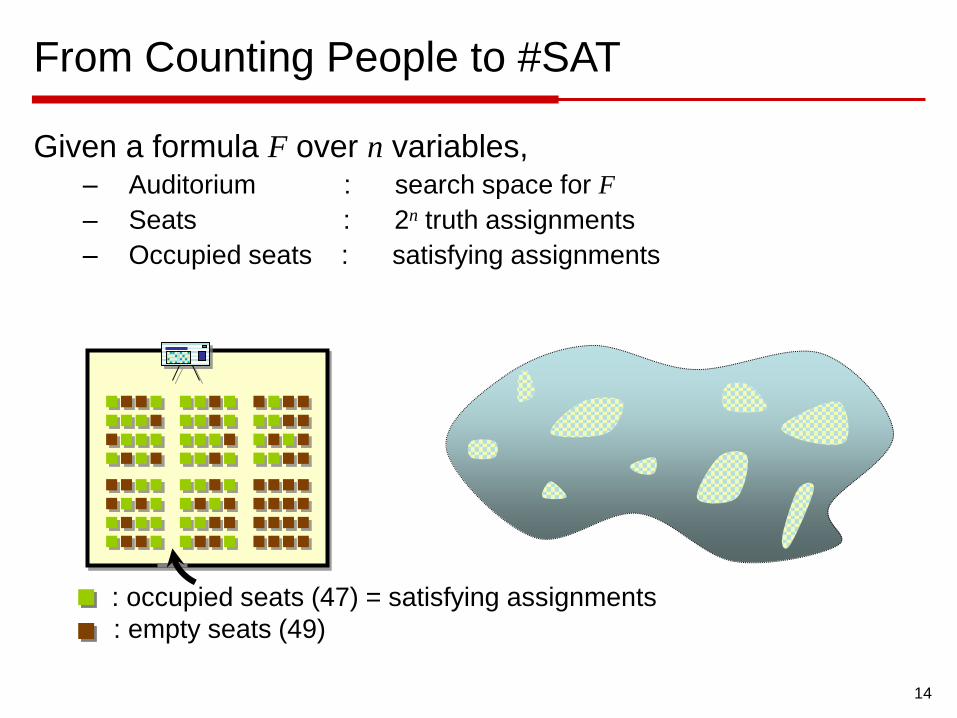
From Counting People to #SAT

Given a formula F over n variables,– Auditorium : search space for F

– Seats : 2n truth assignments

– Occupied seats : satisfying assignments

: occupied seats (47) = satisfying assignments

: empty seats (49)

15

#1: Brute-Force Counting

Idea:

– Go through every seat

– If occupied, increment counter

Advantage:

– Simplicity, accuracy

Drawback:

– Scalability

: occupied seats (47)

: empty seats (49)

16

#2: Branch-and-Bound (DPLL-style)

Idea:

– Split space into sections

e.g. front/back, left/right/ctr, …

– Use smart detection of full/empty

sections

– Add up all partial counts

Advantage:

– Relatively faster, exact

Drawback:

– Still “accounts for” every single

person present: need extremely

fine granularity

– Scalability

Framework used in DPLL-based

systematic exact counters

e.g. Cachet [Sang-et]

See also compilation approaches [Darwiche et. al]

Approximate model counting?

17

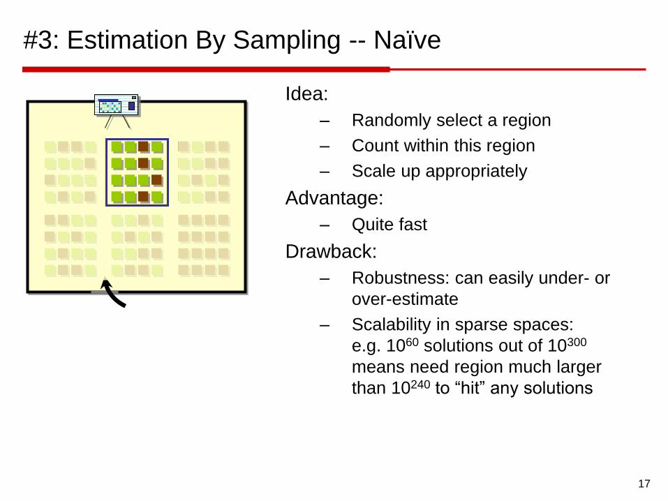
#3: Estimation By Sampling -- Naïve

Idea:

– Randomly select a region

– Count within this region

– Scale up appropriately

Advantage:

– Quite fast

Drawback:

– Robustness: can easily under- or

over-estimate

– Scalability in sparse spaces:

e.g. 1060 solutions out of 10300

means need region much larger

than 10240 to “hit” any solutions

18

A Distributed Coin-Flipping Strategy

(Intuition)

Idea:

Everyone starts with a hand up

– Everyone tosses a coin

– If heads, keep hand up,

if tails, bring hand down

– Repeat till no one hand is up

Return 2#(rounds)

Does this work?

• On average, Yes!

• With M people present, need roughly log2M rounds for

a unique hand to survive

Let’s Try Something Different …

19

Making the Intuitive Idea Concrete

• How can we make each solution “flip” a coin?

– Recall: solutions are implicitly “hidden” in the formula

– Don’t know anything about the solution space structure

• How do we transform the average behavior into a robust

method with provable correctness guarantees?

Somewhat surprisingly, all these issues can be resolved!

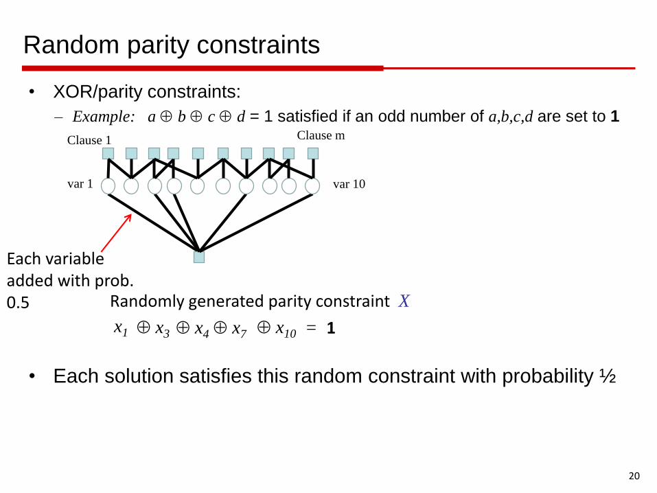
Random parity constraints

• XOR/parity constraints:

– Example: a b c d = 1 satisfied if an odd number of a,b,c,d are set to 1

• Each solution satisfies this random constraint with probability ½

20

Randomly generated parity constraint X

Each variable added with prob. 0.5

x1 x3 x4 x7 x10 = 1

Clause 1 Clause m

var 1 var 10

21

Using XORs for Counting

Given a formula F

1. Add some XOR constraints to F to get F’

(this eliminates some solutions of F)

2. Check whether F’ is satisfiable

3. Conclude “something” about the model count of F

Key difference from previous methods:

o The formula changes

o The search method stays the same (SAT solver)

Streamlined

formula

CNF formula

XOR

constraints

Off-the-shelf

SAT Solver

deduce

model

count

repeat a few times

22

The Desired Effect

M = 50 solutions 22 survive

7 survive

13 survive

3 surviveunique solution

If each XOR cut the solution space roughly in half, would

get down to a unique solution in roughly log2 M steps!

What about weighted counting?

For any configuration (or state), defined by an assignment of values to

the random variables, we can compute the weight/probability of that

configuration.

SPRINKLERRAINWET GRASS

SPRINKLER

True False

RA

INTrue 0.01 0.99

False 0.5 0.5

RAIN

True False

0.2 0.8

Example: Pr [Rain=T, Sprinkler=T, Wet=T] ∝ 0.01 * 0.2 * 0.99

WET

True False

… …

0.99 0.01

… …

Factor “Rain => Sprinkler”“Rain OR Sprinkler => Wet Grass” “Rain”

SPRINKLER

True False

RA

INTrue F T

False T T

24

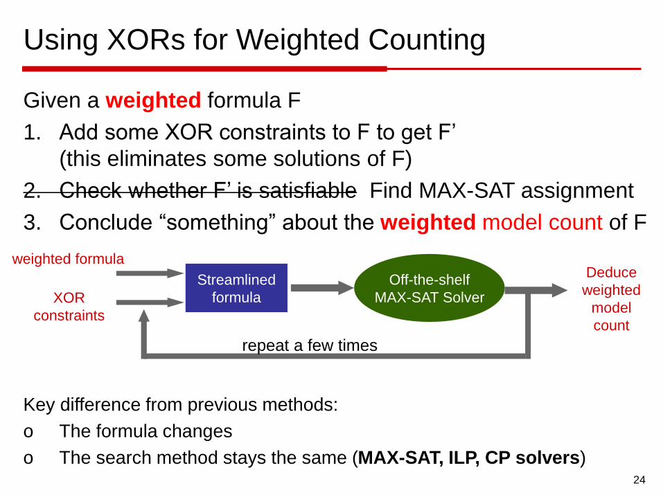
Using XORs for Weighted Counting

Given a weighted formula F

1. Add some XOR constraints to F to get F’

(this eliminates some solutions of F)

2. Check whether F’ is satisfiable Find MAX-SAT assignment

3. Conclude “something” about the weighted model count of F

Key difference from previous methods:

o The formula changes

o The search method stays the same (MAX-SAT, ILP, CP solvers)

Streamlined

formula

weighted formula

XOR

constraints

Off-the-shelf

MAX-SAT Solver

Deduce

weighted

model

count

repeat a few times

Accuracy Guarantees

Main Theorem (stated informally):

With probability at least 1- δ (e.g., 99.9%),

WISH (Weighted-Sums-Hashing) computes a sum defined

over 2n configurations (probabilistic inference, #P-hard)

with a relative error that can be made as small as desired,

and it requires solving θ(n log n) optimization instances

(NP-equivalent problems).

25

Implementations and experimental results

• Many implementations based on this idea (originated from theoretical work due

to [Stockmeyer-83, Valiant-Vazirani-86]):

– Mbound, XorSample [Gomes et al-2007]

– WISH, PAWS [Ermon et al-2013]

– ApproxMC, UniWit,UniGen [Chakraborty et al-2014]

– Achilioptas et al at UAI-15 (error correcting codes)

– Belle et al. at UAI-15 (SMT solvers)

• Fast because they leverage good SAT/MAX-SAT solvers!

• How hard are the “streamlined” formulas (with extra parity constraints)?

26

Sparse/ Low-density parity constraints

The role of sparse (low-density) parity constraints

X = 1 length 1, large variance

X Y = 0 length 2, variance?

X Y Q = 0 length 3, variance?

X Y … Z = 0 length n/2, small variance

The shorter the constraints are, the easier they are to reason about.

The longer the constraints are, the more accurate the counts are

27

Increasingly complex constraints

… Increasingly low variance

Can short constraints actually be used?

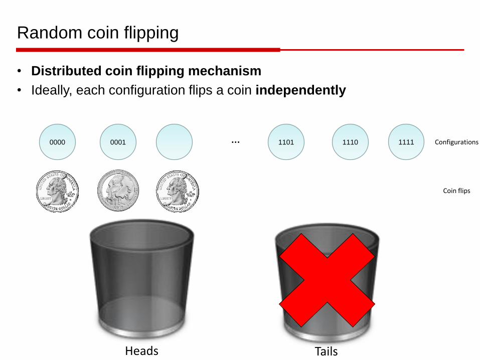
Random coin flipping

• Distributed coin flipping mechanism

• Ideally, each configuration flips a coin independently

0000 … 11110001 1101 1110

Heads Tails

Configurations

Coin flips

• Issue: we cannot simulate so many independent coin flips (one for

each possible variable assignment)

• Solution: each configuration flips a coin pairwise independently

• Any two coin flips are independent

• Three or more might not be independent

Still works! Pairwise independence guarantees that configurations do not

cluster too much in single bucket.

Can be simulated using random parity constraints: simply add each

variable with probability ½.

Pairwise Independent Hashing

…

``Long’’ parity constraints are difficult to deal with!

• New class of average universal hash functions (coin flips generation

mechanism) [ICML-14]

• Pairs of coin flips are NOT guaranteed to be independent anymore

• Key idea: Look at large enough sets. If we look at all pairs, on average

they are “independent enough”. Main result:

1. These coin flips are good enough for probabilistic inference (applies to all

previous techniques based on hashing; same theoretical guarantees)

2. Can be implemented with short parity constraints

Average Universal Hashing

…

Short Parity Constraints for Probabilistic Inference

and Model Counting

Main Theorem (stated informally): [AAAI-16, Sunday]

For large enough n (= number of variables),

– Parity constraints of length log(n) are sufficient.

– Parity constraints of length log(n) are also necessary.

Proof borrows ideas from the theory of low-density parity

check codes.

Short constraints are much easier to deal with in practice.

Can even use other constraints! [under submission]31

Outline

• Introduction and Motivation

– Knowledge representation and reasoning

– Probabilistic modeling and inference

– Model counting and sampling

• Algorithmic approaches

– Unweighted model counting

– Weighted model counting

• Conclusions

32

Conclusions

• SAT solvers had a major impact on AI and other CS fields

• However, there are many interesting problems in AI and

Machine Learning are beyond NP

• Model counting is the prototypical problem for

probabilistic reasoning

– Key computational problem with a long history: early

work dates back to the 50s.

– Recent approaches: try to “reduce” to problems in NP so

that we can leverage SAT/ solvers.

– Provides nice theoretical guarantees, as opposed to

traditional approaches (MCMC, variational)

33