NBER WORKING PAPER SERIES

ERRORS IN PROBABILISTIC REASONING AND JUDGMENT BIASES

Daniel J. Benjamin

Working Paper 25200http://www.nber.org/papers/w25200

NATIONAL BUREAU OF ECONOMIC RESEARCH1050 Massachusetts Avenue

Cambridge, MA 02138October 2018

This chapter will appear in the forthcoming Handbook of Behavioral Economics (eds. Doug Bernheim,Stefano DellaVigna, and David Laibson), Volume 2, Elsevier, 2019. For helpful comments, I am gratefulto Andreas Aristidou, Nick Barberis, Pedro Bordalo, Colin Camerer, Christopher Chabris, SamanthaCherney, Bob Clemen, Gary Charness, Alexander Coutts, Chetan Dave, Juan Dubra, Craig Fox, NicolaGennaioli, Tom Gilovich, David Grether, Zack Grossman, Ori Heffetz, Jon Kleinberg, Lawrence Jin,Annie Liang, Chuck Manski, Josh Miller, Don Moore, Ted O’Donoghue, Jeff Naecker, Collin Raymond,Alex Rees-Jones, Rebecca Royer, Josh Schwartzstein, Tali Sharot, Andrei Shleifer, Josh Tasoff, RichardThaler, Joël van der Weele, George Wu, Basit Zafar, Chen Zhao, Daniel Zizzo, conference participantsat the 2016 Stanford Institute for Theoretical Economics, and the editors of this Handbook, Doug Bernheim,Stefano DellaVigna, and David Laibson. I am grateful to Matthew Rabin for extremely valuable conversationsabout the topics in this chapter over many years. I thank Peter Bowers, Rebecca Royer, and especiallyTushar Kundu for outstanding research assistance. The views expressed herein are those of the authorand do not necessarily reflect the views of the National Bureau of Economic Research.

NBER working papers are circulated for discussion and comment purposes. They have not been peer-reviewed or been subject to the review by the NBER Board of Directors that accompanies officialNBER publications.

© 2018 by Daniel J. Benjamin. All rights reserved. Short sections of text, not to exceed two paragraphs,may be quoted without explicit permission provided that full credit, including © notice, is given tothe source.

Errors in Probabilistic Reasoning and Judgment BiasesDaniel J. BenjaminNBER Working Paper No. 25200October 2018JEL No. D03,D90

ABSTRACT

Errors in probabilistic reasoning have been the focus of much psychology research and are amongthe original topics of modern behavioral economics. This chapter reviews theory and evidence on thistopic, with the goal of facilitating more systematic study of belief biases and their integration intoeconomics. The chapter discusses biases in beliefs about random processes, biases in belief updating,the representativeness heuristic as a possible unifying theory, and interactions between biased beliefupdating and other features of the updating situation. Throughout, I aim to convey how much evidencethere is for (and against) each putative bias, and I highlight when and how different biases may berelated to each other. The chapter ends by drawing general lessons for when people update too muchor too little, reflecting on modeling challenges, pointing to areas of economics to which the biasesare relevant, and highlighting some possible directions for future work.

Daniel J. BenjaminCenter for Economics and Social ResearchUniversity of Southern California635 Downie Way, Suite 312Los Angeles, CA 90089-3332and NBERdaniel.benjamin@gmail.com

Table of Contents Section 1. Introduction ............................................................................................................ 1 Section 2. Biased Beliefs About Random Sequences .............................................................. 9

2.A. The Gambler’s Fallacy and the Law of Small Numbers ................................................. 9 2.B. The Hot-Hand Bias ....................................................................................................... 16 2.C. Additional Biases in Beliefs About Random Sequences ............................................... 21

Section 3. Biased Beliefs About Sampling Distributions .......................................................24

3.A. Partition Dependence.................................................................................................... 24 3.B. Sample-Size Neglect and Non-Belief in the Law of Large Numbers ............................ 33 3.C. Sampling-Distribution-Tails Diminishing Sensitivity ................................................... 41 3.D. Overweighting the Mean and the Fallacy of Large Numbers ....................................... 43 3.E. Sampling-Distribution Beliefs for Small Samples ........................................................ 46 3.F. Summary and Comparison of Sequence Beliefs Versus Sampling-Distribution Beliefs 48

Section 4. Evidence on Belief Updating .................................................................................50

4.A. Conceptual Framework ................................................................................................ 54 4.B. Evidence from Simultaneous Samples .......................................................................... 57 4.C. Evidence from Sequential Samples ............................................................................... 78

Section 5. Theories of Biased Inference .................................................................................86

5.A. Biased Sampling-Distribution Beliefs ........................................................................... 87 5.B. Conservatism Bias ........................................................................................................ 96 5.C. Extreme-Belief Aversion ............................................................................................... 98 5.D. Summary .....................................................................................................................102

Section 6. Base-Rate Neglect ................................................................................................ 104 Section 7. The Representativeness Heuristic ....................................................................... 116

7.A. Representativeness ......................................................................................................116 7.B. The Strength-Versus-Weight Theory of Biased Updating ...........................................122 7.C. Economic Models of Representativeness ....................................................................125 7.D. Modeling Representativeness Versus Specific Biases .................................................134

Section 8. Prior-Biased Inference ........................................................................................ 136

8.A. Conceptual Framework ...............................................................................................136 8.B. Evidence and Models ...................................................................................................138

Section 9. Preference-Biased Inference ............................................................................... 149

9.A. Conceptual Framework ...............................................................................................149 9.B. Evidence and Models ...................................................................................................151

Section 10. Discussion........................................................................................................... 158

10.A. When Do People Update Too Much or Too Little? ...................................................158 10.B. Modeling Challenges ................................................................................................160

10.C. Generalizability from the Lab to the Field ................................................................163 10.D. Connecting With Other Areas of Economics ............................................................167 10.E. Some Possible Directions For Future Research .......................................................169

1

Section 1. Introduction

Probabilistic beliefs are central to decision-making under risk. Therefore,

systematic errors in probabilistic reasoning can matter for the many economic decisions

that involve risk, including investing for retirement, purchasing insurance, starting a

business, and searching for goods, jobs, or workers. This chapter reviews what

psychologists and economists have learned about such systematic errors. At the cost of

some precision, throughout this chapter I will use the term “belief biases” as shorthand for

“errors in probabilistic reasoning.” By “bias,” in this chapter I will mean any deviation

from correct reasoning about probabilities or Bayesian updating.1

This chapter’s area of research—which is often called “judgment under

uncertainty” or “heuristics and biases” in psychology—was introduced by the psychologist

Ward Edwards and his students and colleagues in the 1960s (e.g., Phillips and Edwards,

1966). This topic was the starting point of the collaboration between Daniel Kahneman and

Amos Tversky. Their seminal early papers (e.g., Tversky and Kahneman, 1971, 1974)

jumpstarted an enormous literature in psychology and influenced thinking in many other

disciplines, including economics.

Despite so much work by psychologists and despite being one of the original topics

of modern behavioral economics, to date belief biases have received less attention from

behavioral economists than time, risk, and social preferences. Belief biases have also made

1 My use of the same term “bias” for all of these deviations is not meant to obscure the distinctions between them in terms of their psychological origins. For example, the gambler’s fallacy (the belief that heads is likely to be followed by tails; Section 2.A) is a mistaken mental model of independent random processes, while Non-Belief in the Law of Large Numbers (the belief that the distribution of a sample mean is independent of sample size; Section 3.B) is a failure to understand or apply a deep statistical principle. These differences can matter, for example, for who makes the errors, under what circumstances, and the likelihood that interventions could reduce the bias.

2

few inroads in applied economic research, with the important exception of behavioral

finance (see Chapters XXX (by Barberis) and XXX (by Malmendier) of this Handbook). I

suspect that is because in many available datasets, beliefs have been unobserved. But today,

datasets are becoming much more plentiful, and it is easier than ever to collect one’s own

data. Therefore in my view, the relative lack of attention paid to belief biases makes them

an especially exciting area of research, rife with opportunities for innovative work. For

some topics in this chapter, particularly beliefs about random sequences (Section 2) and

prior-biased updating (Section 8), the body of evidence and theory is relatively mature. For

these topics, the biases could be fairly straightforwardly incorporated into applied

economic models or explored in new empirical settings. For other topics, such as many

aspects of beliefs about sample distributions (Section 3) and features of biased inference

(Section 5), there are basic questions about what the facts are and how to model them that

remain poorly addressed. For those topics, careful experimental work and modeling could

fundamentally reshape how these biases are understood.

This chapter has three specific goals. First, I have tried to organize the topics in a

natural way for economists. For example, I review biased beliefs about random samples

before discussing biased inferences because, according to the standard model in economics,

beliefs about random samples are a building block for inference. I hope that this

organization will facilitate more systematic study of the biases and integration into

economics.

Second and relatedly, I have tried to highlight when and how different biases may

be related to each other. For example, some of the biases about random samples may

underlie some of the biases about inferences. Sometimes, belief biases are presented in a

3

way that makes them seem like an unmanageable laundry list of unrelated items. By

emphasizing possible connections, I hope to point researchers in the direction of a smaller

number of unifying principles. At the same time, I have tried to highlight when different

biases may push in opposite directions or even jointly imply logically inconsistent beliefs,

cases which raise interesting challenges for modeling and applications.

Third, I have tried to convey how much evidence there is for (and against) each

putative bias. Often, papers focused on a particular bias review existing evidence somewhat

selectively. While it is impossible to be comprehensive, and while I have surely missed

papers inadvertently, for each topic I attempted to find as many papers as I could that

provide relevant evidence from both economics and psychology. In some cases, I was

surprised by what I learned. For example, as discussed in Section 4, the evidence

overwhelmingly indicates that people tend to infer too little from signals rather than too

much, even from small samples of signals. Another example is discussed in Section 9:

while discussions of the literature often take for granted that people update their beliefs

more in response to good news than bad news, and while the psychology research is nearly

unanimously supportive, the evidence from experimental economics taken as a whole is

actually rather muddy, and it leaves me puzzled as to whether and under what

circumstances there is an asymmetry.

For each bias, in addition to discussing the most compelling evidence for and

against it, which is usually from laboratory experiments, I also try to highlight the most

persuasive field evidence and existing models of the bias. While I mention modeling

challenges as they arise, I return in Section 10 to briefly discuss some of the challenges

common to many of the belief biases.

4

Due to space constraints, I cannot cover all belief biases, or even most of them.2

The biases I focus on all relate to beliefs about random samples and belief updating. I chose

these topics because they are core issues for most applications of decision making under

risk, they allow the chapter to tell a fairly coherent narrative, and some of them have not

been well covered in other recent reviews. In addition, admittedly, this chapter is tilted

toward topics I am more familiar with.

An especially major omission from this chapter is “overconfidence,” which is

probably the most widely studied belief distortion in economics to date and is discussed at

some length in Chapters XXX (by Barberis) and XXX (by Malmendier) of this Handbook.

The term “overconfidence” is unfortunately used to refer to several distinct biases—and

for the sake of clarity, I advocate adopting terminology that distinguishes between distinct

meanings. One meaning is overprecision, a bias toward beliefs that are too certain (for

reviews, see Lichtenstein, Fischhoff, and Phillips, 1982, and Moore, Tenney, and Haran,

2015). Relatedly, the biased belief that one’s own signal is more precise than others’ signals

has been argued to be important for understanding trading in financial markets (e.g.,

Daniel, Hirshleifer, and Subrahmanyam, 1998), as well as for social learning and voting;

this bias is discussed in Chapter XXX (by Eyster) of this Handbook, which addresses biases

in beliefs about other people.3 Another meaning is overoptimism, a bias toward beliefs that

2 Moreover, because this chapter is organized around specific biases, it omits discussion of related work that is less tightly connected to the psychological evidence. For example, Barberis, Shleifer, and Vishny (1998) is among the seminal papers that incorporated belief biases into an economic model. Yet it is only barely mentioned in this chapter because its core assumption—that stocks switch between a mean-reverting state and a positively autocorrelated state—does not fit neatly with the evidence on people’s general beliefs about i.i.d. processes (described in Section 2). 3 While the key feature of this bias is the relative precision of one’s own versus others’ signals, models of the bias typically assume that agents believe that their own signal is more precise than it is, and therefore agents overinfer from their own signal. Relevantly for such models, the evidence reviewed in Section 4 of this chapter indicates that people generally underinfer rather than overinfer (see also Section 10.A). Therefore, it would be more realistic to assume that agents underinfer from their own signal, even if they believe that others observe less precise signals (and thus infer even less than they do).

5

are too favorable to oneself (a classic early paper is Weinstein, 1980; for a review, see

Windschitl and O’Rourke, 2015). Although I do not discuss overoptimism in this chapter,

biases in belief updating, in particular those reviewed in Sections 5.A, 6, and 8, are relevant

to how overoptimistic beliefs are maintained in the face of evidence. A closely related

omission is motivated beliefs, an important class of biases related to having preferences

over beliefs (a classic review is Kunda, 1990; for a recent review, see Bénabou and Tirole,

2016). While I do not discuss the broad literature on motivated beliefs, preference-biased

updating (reviewed in Section 9) is considered to be one potential mechanism that helps

people end up with the beliefs they want.

Other omissions from this chapter include: vividness bias, according to which

hearing an experience described more vividly, or experiencing it oneself, may cause it to

have a greater impact on one’s beliefs (e.g., Nisbett and Ross, 1980; an early review is

Taylor and Thompson, 1982, which concludes that the evidence is not strong; for a recent

meta-analysis, see Blondé and Girandola, 2016); and hindsight bias, according to which,

ex post, people overestimate how much they and others knew ex ante (Fischhoff, 1975; for

a recent review, see Roese and Vohs, 2012, and for an economic model, see Madarász,

2012). I do not review the evidence on how people draw inferences from samples about

population means, proportions, variances, and correlations (for reviews, see Peterson and

Beach, 1967; Juslin, Winman, and Hansson, 2007).4 I also do not cover the availability

heuristic, according to which judgments about the likelihood of an event is influenced by

4 Recent work in this vein has concluded that people tend to overlook selection biases and treat sample statistics as unbiased estimators of population statistics (Juslin, Winman, and Hansson, 2007). Much of the economics research on errors in strategic reasoning has focused on such failure to account for selection bias (see Chapter XXX (by Eyster) of this Handbook). In the experimental economics literature, Enke (2017) recently explored this error in a non-strategic setting.

6

how easily examples or instances come to mind (Tversky and Kahneman, 1974; for a

review, see Schwarz and Vaughn, 2002), but Gennaioli and Shleifer’s (2010) model of

representativeness, discussed in Section 7.C of this chapter, is related to it.

Although some of the biases in this chapter might be understood as people not

paying attention to relevant aspects of a judgment problem, I do not review the literature

on inattention since that is the focus of Chapter XXX (by Gabaix) of this Handbook. I also

do not at all address biases in probabilistic beliefs about other people or their behavior.

Many of those biases are covered in Chapter XXX (by Eyster) of this Handbook. However,

in Section 10 of this chapter, I briefly mention some of the modeling challenges that arise

when applying the biases discussed here in environments with strategic interaction.

I will also not separately discuss the sprawling literature on “debiasing”—which

refers to interventions designed to reduce biases—although some of this work will come

up in the context of specific biases. Debiasing strategies come in three forms (Roy and

Lerch, 1996): (i) modifying the presentation of a problem to elicit the appropriate mental

procedure; (ii) training people to think correctly about a problem; and (iii) doing the

calculations for people, so that they merely need to provide the inputs to the calculations.

The classic review is Fischhoff (1982), and a more recent review is Ludolph and Schulz

(2017). Some recent work has suggested that instructional games may be more effective

than traditional training methods at persistent debiasing that generalizes across decision

making contexts (Morewedge et al., 2015).

While I mention throughout the chapter when belief elicitation was incentivized, I

do not discuss the literature on how to elicit beliefs in an incentive-compatible way. For a

recent review, see Schotter and Trevino (2014).

7

There are a number of literature reviews that partially overlap the material covered

in this chapter. Some of these are oriented around belief updating and are therefore similar

to this chapter in terms of topics covered (Peterson and Beach, 1967; Edwards, 1968;

DuCharme, 1969; Slovic and Lichtenstein, 1971; Grether, 1978; Fischhoff and Beyth-

Marom, 1983). Others are reviews of the behavioral decision research literature more

broadly that have substantial sections devoted to biases in probabilistic beliefs (Rapoport

and Wallsten, 1972; Camerer, 1995; Rabin, 1998; DellaVigna, 2009). Relative to this

chapter, Dhami (2017, Part VII, Chapter 1) is a textbook-style treatment that covers a much

broader range of judgment biases but in less depth. This chapter builds on and updates

these earlier reviews. For the biases it addresses, this chapter aims to broadly cover the

available evidence from both psychology and economics with an eye toward formal

modeling and incorporation into economic analyses.

The chapter has five parts and is organized as follows. The first part examines

biased beliefs about random processes: Section 2 is about sequences (e.g., a sequence of

coin flips), and Section 3 is about sampling distributions (e.g., the number of heads out of

ten flips). An overarching theme is that, while some biases about sampling-distribution

beliefs seem to result from biases in beliefs about sequences, there are additional biases

that are specific to sampling-distribution beliefs. The second part of the chapter examines

biases in belief updating. On the basis of a review and meta-analysis of the experimental

evidence, Section 4 lays out a set of stylized facts. The central lesson is that people

underweight both the information from signals and their priors—errors that I refer to as

underinference and base-rate neglect, respectively. Section 5 discusses the three main

theories of underinference, and Section 6 discusses base-rate neglect. The third part of the

8

chapter is Section 7, which focuses on the representativeness heuristic, generally

considered to be a unifying theory for many of the biases discussed earlier in the chapter.

I highlight that the representativeness heuristic has several distinct components and that

efforts to formalize it have focused on one component at a time. At the end of the section,

I reflect on the merits of modeling the representativeness heuristic as opposed to specific

biases. The fourth part of the chapter examines interactions between biased updating and

other features of the updating situation. Section 8 focuses on a type of confirmation bias I

call “prior-biased updating,” according to which people update less when the signal points

toward the opposite hypothesis as their prior. Section 9 reviews the evidence on what I call

“preference-biased updating,” which posits that people update less when the signal favors

their less-preferred hypothesis. The final part of the chapter is Section 10, which draws

general lessons from the chapter as a whole, reflects on challenges in this area of research,

advocates for connecting better to field evidence and other areas of economics, and

highlights some possible directions for future work.

9

Section 2. Biased Beliefs About Random Sequences

2.A. The Gambler’s Fallacy and the Law of Small Numbers

The gambler’s fallacy (GF) refers to the mistaken belief that, in a sequence of

signals known to be i.i.d., observing one signal reduces the likelihood of next observing

that same signal. For example, people think that when a coin flip comes up heads, the next

flip is more likely to come up tails.

The GF has long been observed among gamblers and is one of the oldest

documented biases. Laplace (1814), who anticipated much of the literature on errors in

probabilistic reasoning (Miller and Gelman, 2018), described people’s belief that the

fraction of boys and girls born each month must be roughly balanced, so that if more of

one sex has been born, the other sex becomes more likely. The first systematic study of the

GF was Alberoni (1962a,b), who reported many experiments showing that, with i.i.d.

binomial signals, people think a streak of a signals is less likely than a sequence with a mix

of a and b signals.5

Rabin (2002) and Oskarsson, Van Boven, McClelland, and Hastie (2009) provided

reviews of the extensive literature documenting the GF in surveys and experiments. While

most of this evidence comes from undergraduate samples, Dohmen, Falk, Huffman,

Marklein, and Sunde (2009) surveyed a representative sample of the German population,

asking about the probability of a head following the sequence TTTHTHHH. While 60% of

5 Laplace (1814) and Alberoni (1962a,b) both provided explanations of the GF that anticipated Tversky and Kahneman’s (1971) theory, the Law of Small Numbers, which is discussed below. Specifically, Laplace conjectured that the GF results from misapplying the logic of sampling without replacement, which is exactly the intuition captured by Rabin’s (2002) model of the Law of Small Numbers, also discussed below. Alberoni’s “Principle of the Best Sample” is essentially a restatement of Tversky and Kahneman’s description of the Law of Small Numbers: “[People believe that the most likely] sample is that which, without presenting a cyclic structure, reflects the composition of the system of expectations in the whole and in each of its parts” (Alberoni, 1962a, p. 253).

10

the sample gave the correct answer of 50%, the GF was the dominant direction of bias,

with 21% of the sample giving answers less than 50% and 9% of the sample giving answers

greater than 50%.

Rabin (2002) pointed out ways in which some of the laboratory evidence is not

fully compelling. For example, in experiments involving coin flips (or other 50-50

binomial signals) that ask participants to guess the next flip in a sequence, either guess has

an equal chance of being correct. Moreover, many of the experiments are unincentivized.

However, there have been experiments that address these concerns. For example,

Benjamin, Moore, and Rabin (2018) conducted two incentivized experiments in which they

elicited participants’ beliefs about the probability of a head following streaks of heads of

each possible length up to 9. Like Dohmen et al., they found that the majority of reported

beliefs were the correct answer of 50%, but the incorrect answers predominantly exhibited

the GF. On average, their participants (undergraduates and a convenience sample of adults)

assessed a 44% to 50% chance that a first flip would be a head but only a 32% to 37%

chance that a flip following 9 heads would be a head.6

Most field evidence of behavior consistent with the GF is from gambling settings,

such as dog- and horse-race betting (Metzger, 1985; Terrell and Farmer, 1996), roulette

playing in casinos (Croson and Sundali, 2005), and lottery-ticket purchasing (e.g.,

6 Miller and Sanjurjo (2018) pointed out conditions under which GF-like beliefs are actually correct rather than being a bias. Specifically, fixing an i.i.d. sequence, say, a sequence of coin flips, and any streak length, they show that the (true) frequency of a head following a streak of heads within that sequence is less than 50%. Moreover, this frequency is decreasing in the streak length. Roughly speaking, the reason is that the expected frequency of heads in the entire sequence is 50%, so knowing that some of the flips are heads makes it more likely that the others are tails. Miller and Sanjurjo’s result, however, is not relevant for much of the evidence on the GF. For example, Dohmen et al. and Benjamin, Moore, and Rabin asked about the probability of a head following a specific sequence of flips, questions for which the correct answer is always 50%. Miller and Sanjurjo’s result is relevant for evidence of the hot-hand bias, however, as discussed in Section 2.B.

11

Clotfelter and Cook, 1993; Terrell, 1994). For example, using individual-level

administrative data from the Danish national lottery, Suetens, Galbo-Jørgensen, and Tyran

(2016) found that players placed roughly 2% fewer bets on numbers that won in the

previous week.

Chen, Moskowitz, and Shue (2016) examined three other field settings: judges’

decisions in refugee asylum court, reviews of loan applications, and umpires’ calls on

baseball pitches. In all three settings, they found that decision making is negatively

autocorrelated, controlling for case quality. For example, even though the quality of referee

asylum cases appears to be serially uncorrelated conditional on observables, Chen et al.

estimated that a judge is up to 3.3% more likely to deny asylum in the current case if she

approved it in the previous case. To explain their findings, Chen et al. theorized that judges

think of underlying case quality as an i.i.d. process and thus, due to the GF, when the

previous case was (say) positive, the decision maker’s prior belief about underlying case

quality is negative for the next case. This prior belief then influences the decision in the

next case. While Chen et al. persuasively ruled out a number of alternative explanations,

they acknowledged that they cannot rule out “sequential contrast effects” (e.g., Pepitone,

and DiNubile, 1976; Simonsohn, 2006; Bhargava and Fisman, 2014), in which the decision

maker’s perception of (rather than belief about) case quality is influenced by the previous

case.

A related literature in economics examines whether people randomize when

playing a game that has a unique Nash equilibrium in mixed strategies. Equilibrium play

requires that the sequence of actions be unpredictable and hence serially independent, but

in laboratory games, experimental participants often alternate actions more often than they

12

should (for a review, see Rapoport and Budescu, 1997). In the largest field study to date,

Gauriot, Page, and Wooders (2016) analyzed data on half a million serves made by

professional tennis players and find that players switch their direction too often (see also

Walker and Wooders, 2001; Hsu, Huang, and Tang, 2007). This excessive switching could

reflect the mistaken GF intuition for what random sequences look like.

As an explanation of the GF, Tversky and Kahneman (1971) proposed that “people

view a sample randomly drawn from a population as highly representative, that is, similar

to the population in all essential characteristics” (p. 105). They called this mistaken

intuition a belief in the “Law of Small Numbers” (LSN), a tongue-in-cheek name which

conveys the idea that people believe that the Law of Large Numbers applies also to small

samples.7 Tversky and Kahneman highlighted two implications of the LSN. First, it

generates the GF: after (say) a streak of heads, a tail is needed to ensure that the overall

sequence reflects the unbiasedness of the coin. Second, belief in the LSN should cause

people to infer too much from small samples.

There is very little evidence in support of the latter prediction. The evidence

Tversky and Kahneman presented was from surveys of academic psychologists showing

that they underestimate sampling variation and expect statistically significant results

obtained in small samples to replicate at unrealistically high rates. For example, they

described to their survey respondents an experiment with 15 participants that obtained a

statistically significant result (p < 0.05) with t = 2.46. If a subsequent experiment with 15

more participants obtained a statistically insignificant result in the same direction with t =

7 To help flesh out the LSN, Bar-Hillel (1982) directly asked experimental participants to judge the “representativeness” of different samples. She found that their judgments were influenced by a variety of factors. For example, a sample was judged to be more representative if its mean matched the population mean and if none of the sample observations were repeats.

13

1.70, most of Tversky and Kahneman’s respondents said they would view that result as a

“failure to replicate”—even though the second result is more plausibly viewed as

supportive. However, as Oakes (1986) discussed, the interpretation of this evidence in

terms of the LSN is confounded by other errors in understanding statistics, including a

heuristic of treating results that cross the statistical significance threshold as much more

likely to reflect “true” effects than they do. In additional surveys of academic

psychologists, Oakes found that his respondents exhibited similar overinference from

statistically significant results obtained in larger samples, indicating that the

misinterpretations are not specific to small samples. Moreover, as discussed in Section 4

of this chapter, the experimental evidence on inference taken as a whole suggests that even

in small samples, people generally underinfer rather than overinfer.

Rabin (2002) proposed a formal model of the LSN (see also Rapoport and Budescu,

1997, for a model of the belief that i.i.d. processes tend to alternate). Signals are known to

be drawn i.i.d., with a signals having rate θ and b signals having rate 1-θ. Because the

agent is a believer in the LSN, she forms beliefs as if the signals are drawn without

replacement from an urn of finite size M containing θM a signals (where θM is assumed

to be an integer). The model directly generates the GF: after (say) an a signal is drawn,

there is one fewer a signal in the urn, so the probability that the next signal is a is ,

which is smaller than θ.

When the true rate is unknown and must be inferred by the agent, the model implies

that the agent will err in the direction of overinference, ending up with a posterior belief

that is too extreme. For example, suppose there are two states of the world: in state A, the

rate of a signals is high ( ), whereas in state B, it is low ( ). The agent thinks the

θM −1M −1

θ A θB <θ A

14

probability of aa is if the state is A and if the

state is B. While the agent thinks a streak such as aa is less likely than it is regardless of

the state, the agent thinks it is especially unlikely in state B since .

Consequently, the agent interprets aa as stronger evidence in favor of state A than it truly

is. In Rabin’s example, if the agent thinks an average fund manager has a 50% chance of

success in each year, then he thinks a manager with two consecutive successful years is

unusually good.8

This overinference in turn implies that, when the agent observes a small number of

signals from many sources, she exaggerates the amount of variation in rates across sources.

For example, suppose all fund managers are average, and the agent observes the last two

years of performance for many managers. Because the agent underestimates how often

average managers will have consecutive good or bad years, she will think the number of

fund managers with such consecutive years is inconsistent with all managers being average

and will instead conclude that there must be a mix of good and bad managers.

This model is useful for straightforwardly elucidating this and other basic

implications of belief in the LSN. However, Rabin highlights that the model has artificial

features that limit its suitability for many applications; for example, since the urn only

contains M signals, the urn must be “renewed” at some point in order for the model to make

predictions about sequences longer than length M. To address these limitations, Rabin and

8 Although Rabin’s (2002) model generates both the GF and overinference, given the lack of evidence for the latter, it is worth noting that overinference does not necessarily follow from the belief in the GF. The GF for a signals entails that and . Overinference after two a

signals entails that , but this is not implied by the GF inequalities.

π (aa | A) = θ A ⋅θ AM −1M −1

⎛⎝⎜

⎞⎠⎟

π (aa | B) = θB ⋅θBM −1M −1

⎛⎝⎜

⎞⎠⎟

π (aa | B)π (aa | A)

<θBθ A

⎛

⎝⎜⎞

⎠⎟

2

π (a Ɉa,A) < π (a Ɉ A) π (a Ɉa,B) < π (a Ɉ B)π (a Ɉa,A)π (a Ɉa,B)

< π (a Ɉ A)π (a Ɉ B)

15

Vayanos (2010) introduced a more generally applicable model of belief in the LSN (see

also Teguia, 2017, for a related model in a portfolio-choice setting).

While both the Rabin (2002) and Rabin and Vayanos (2010) models describe the

GF, they do not fully capture the psychology of the LSN that any sample should be

representative of the population. Benjamin, Moore, and Rabin (2018) illustrated this point

in an experiment regarding beliefs about coin flips. They generated a million sequences of

a million coin flips and had participants make incentivized guesses about how often

different outcomes occurred. In some questions, they randomly chose a location in the

sequence (e.g., the 239,672nd flip out of the 1 million) and asked participants to guess how

often, when there had been a streak of 1, 2, or 5 consecutive heads at that location, the next

flip was a head. Participants’ mean probabilities were 44%, 41%, and 39%, consistent with

the GF. In other questions, Benjamin, Moore, and Rabin randomly chose 1, 2, or 5 non-

consecutive flip locations in the sequence at random and asked participants to guess how

often, when all of these flips had been heads, another randomly chosen flip would be a

head. Participants’ mean probabilities—45%, 42%, and 41%—were nearly the same as

those for consecutive flips. Since these flips are non-consecutive, the Rabin (2002) and

Rabin and Vayanos (2010) models do not predict any GF. In fact, Benjamin et al. proved

that whenever a sequence of flip locations is chosen i.i.d., the resulting sequence of flips

must be i.i.d. regardless of whether the flips themselves are serially dependent. Therefore,

no model of the LSN in which an agent’s beliefs are internally consistent could explain

why people expect negative autocorrelation in flips from random locations. Section 10.B

of this chapter contains a brief general discussion of some of the conceptual and modeling

challenges raised by belief biases that generate internally inconsistent beliefs.

16

2.B. The Hot-Hand Bias

The term “hot hand” comes from basketball. A basketball player is said to have a

hot hand when she is temporarily better than usual at making her shots. The term has come

to be used more generally to describe a random process in which outcomes sometimes enter

a “hot” state and have temporarily higher probability than normal. Regardless of whether

a process actually has a hot hand, the “hot-hand bias” is when people believe the process

has more of a hot hand than it does. An agent with the bias will have an exaggerated

expectation that a streak of an outcome will continue because a streak is indicative that the

outcome is hot.

The cleanest evidence for hot-hand bias comes from settings where people believe

in a hot hand even though the outcomes are known to be i.i.d. (a case sometimes called the

“hot-hand fallacy”). For example, as pointed out originally by Laplace (1814), lottery

players place more bets on numbers that have won repeatedly in the recent past, implying

that they mistakenly believe in a hot hand (e.g., Suetens, Galbo-Jørgensen, and Tyran,

2016; see Croson and Sundali, 2005, for evidence from roulette, and Camerer, 1989, and

Brown and Sauer, 1993, for evidence from sports betting markets). This bias appears prima

facie to be the opposite of the GF because the GF says that numbers that won recently are

believed to be less likely to win again. Empirically, Suetens, Galbo-Jørgensen, and Tyran

(2016) found evidence for both: after a lottery number won once, players bet less on it, but

when a streak of two or more wins occurred, players bet more the longer the streak.

Theoretically, Gilovich, Vallone, and Tversky (1985) and others have argued not only that

the two biases co-exist but that the hot-hand bias is a consequence of the GF: to someone

17

who suffers from the GF, an i.i.d. process looks like it has too many streaks, so a belief in

the hot hand arises to explain the apparent excess of streaks.

Rabin and Vayanos (2010) formally developed this argument that hand-hand bias

can arise from belief in the GF. Rabin and Vayanos assumed that an agent dogmatically

believes that one component of the process is negatively correlated, as per the GF, but puts

positive probability (even if very small) on the possibility that the process has a hot hand.

After observing an i.i.d. process for a sufficiently long time and updating Bayesianly about

the probability of a hot state, the agent will come to believe with certainty that there is a

hot state. With the resulting combined GF/hot-hand beliefs, the agent will expect high-

frequency negative autocorrelation, but will expect positive autocorrelation once a long

enough streak has occurred. Applying their model to investors’ beliefs about i.i.d. stock

returns, Rabin and Vayanos argued that it explains several puzzles in finance, such as why

investors believe that stock returns are partially predictable and hence active mutual fund

managers can outperform the stock market.

This theory of hot-hand bias coexisting with and arising from the GF is consistent

with several observations. First, Suetens, Galbo-Jørgensen, and Tyran’s (2016) evidence

mentioned above—that lottery players bet less on a number after it comes up once but more

after a streak—fits the theory nicely. Moreover, Suetens, Galbo-Jørgensen, and Tyran

(2016) found that the lottery players exhibiting the hot-hand bias also tend to be those

exhibiting the GF. Second, Asparouhova, Hertzel, and Lemmon (2009) found that when

experimental participants are asked to predict the next outcome of a process and are not

informed that the process is i.i.d., they predict reversals of single outcomes and

continuation of streaks, again the pattern implied by the theory. Finally, for random

18

processes whose i.i.d. nature is arguably well understood by people (such as coin flips and

roulette spins), the GF is by far the dominant belief. For example, as mentioned in Section

2.A, Benjamin, Moore, and Rabin (2018) asked participants the probability of a head

following streaks of different lengths up to 9 heads and found that the perceived likelihood

of a head is declining monotonically in the length of the streak. The theory of hot-hand bias

arising from the GF implies that for a random process where people put near-zero prior

probability on the existence of the hot hand, the hot-hand bias should not arise—unless

people observe the process for a very long time. Consistent with this, over 1000 draws of

binary i.i.d. processes, Edwards (1961a) found that experimental participants predicted

reversals of streaks for the first 200 draws (see also Lindman and Edwards, 1961) but

continuation of streaks for the last 600 draws.

On the other hand, Guryan and Kearney’s (2008) finding of a “lucky store effect”

may be a challenging observation for the theory. In data on weekly lottery drawings from

Texas, they found that stores that sold a winning ticket sold substantially more tickets in

subsequent weeks, with the effect persisting for up to 40 weeks. This seems to be a case of

hot-hand bias without the GF. As a possible reconciliation with the theory, Guryan and

Kearney speculated that in this context, lottery players might have a strong prior on a hot

hand, for example, because of a belief in the store clerk’s karma.

In the psychology literature, a variety of factors have been proposed to explain

when the GF versus hot-hand bias occurs (Oskarsson, Van Boven, McClelland, and Hastie,

2009). For example, Ayton and Fischer (2004) found that experimental participants

anticipated negative autocorrelation in roulette spins but positive autocorrelation for

successes in human prediction of the outcomes of roulette spins. They proposed that the

19

GF dominates for natural processes, whereas the hot-hand bias dominates when human

performance is involved (see also Caruso, Waytz, and Epley, 2010). While this theory

cannot explain evidence of the GF after a single outcome and the hot-hand bias after a

streak as in Suetens, Galbo-Jørgensen, and Tyran (2016), it is complementary with Rabin

and Vayanos’s model insofar as it provides a theory to explain people’s prior probability

of a hot hand, which is taken as exogenous in Rabin and Vayanos’s model.

Much of the field evidence on the hot hand comes from professional sports.

Identifying a hot-hand bias in such settings is tricky because sports performance is typically

not i.i.d. Since confidence, anxiety, focus, and fatigue vary over time, a true hot hand is

plausible, as is its opposite, a cold hand. Yet accurately estimating the magnitude of a true

hot hand in performance is itself challenging for several reasons, including that

performance affects outcomes only probabilistically (Stone, 2012) and that endogenous

responses by the other team may counteract positive autocorrelation in a player’s

performance (e.g., Rao, 2009). Bar-Eli, Avugos, and Raab (2006) reviewed the sizeable

literature testing for a true hot hand in a variety of sports.

Gilovich, Vallone, and Tversky’s (1985) seminal paper introducing the hot-hand

bias focused on the context of basketball. The paper attracted a lot of attention because it

made a surprising empirical claim: contrary to strongly held beliefs of fans, players, and

coaches, there is not a hot hand in basketball. Gilovich et al. made this claim on the basis

of evidence from three studies. First, they analyzed the shot records of 9 players from a

National Basketball Association (NBA) team over a season and found no evidence of

positive autocorrelation for any of the players. Second, they analyzed the free-throw

records of 9 players from another NBA team and, again, found no evidence of

20

autocorrelation. Finally, they ran a shooting experiment with 26 collegiate basketball

players and found evidence of positive autocorrelation for only one player. They also

found, in incentivized bets, that both shooters and observers expected positive

autocorrelation, but in fact neither shooters nor observers could predict the shooters’

performance better than chance. From the contrast between the widespread belief in the

hot hand and the absence of it in the data, Gilovich et al. inferred that beliefs are biased.

Subsequent work replicated and extended Gilovich et al.’s findings (e.g., Koehler and

Conley, 2003; Avugos, Bar-Eli, Ritov, and Sher, 2013).

Miller and Sanjurjo (2014, 2017) recently identified a subtle statistical bias in

earlier analyses that overturns the conclusion of no hot hand in basketball. Put simply,

Gilovich et al. and others had inferred that there is no true hot hand because the empirical

frequency of making a second shot in a row, (hit|hit), is roughly equal to the

unconditional frequency of making a shot, (hit). While the details vary with the statistical

method, roughly speaking, (hit|hit) is estimated as the ratio of two empirical frequencies:

(hit then hit) / (hit). But when making shots is i.i.d., (hit then hit) and (hit) are

positively correlated in a finite sample. Consequently, (hit|hit) is biased downward

relative to the true conditional probability, p(hit|hit) (Rinott and Bar-Hillel, 2015). Thus,

the evidence that (hit|hit) is roughly equal to (hit) implies that the true probability

p(hit|hit) is actually greater than p(hit). In re-analyses of earlier data, Miller and Sanjurjo

(2014, 2017) found that this bias is substantial. Correcting for the bias, they concluded that

there is evidence for a hot hand in basketball. In a new shooting experiment with many

more shots per participant, Miller and Sanjurjo (2014) again concluded that many players

have a hot hand. Miller and Sanjurjo (2017) re-analyzed Gilovich et al.’s betting data,

p

p

p

p p p p

p

p p

21

pooling across bettors to increase power, and concluded that overall, the bettors did predict

shooters’ performance better than chance. By showing that there is a hot hand, these new

analyses and evidence re-opens—but does not answer—the key question of whether there

is a hot-hand bias in basketball, i.e., a belief in a stronger hot hand than there really is.

In two other sports, recent papers found both a true hot hand and evidence for a

bias. Among Major League Baseball players, Green and Zwiebel (2017) found that recent

performance predicts subsequent performance for both batters and pitchers, and the

magnitudes are substantial (although the analysis did not control for player-ballpark

interaction effects, which can be important in baseball). However, pitchers overreact to

recent good performance by batters, indicating that they believe that the hot hand is

stronger than it is. For example, they walk batters who have recently been hitting home

runs more than can be justified based on the batters’ hot hand. Among players in the World

Darts Championship, Jin (2018) found a substantial hot hand but also found that players’

willingness to take a high-risk/high-reward shot increases by more than it should in light

of their hot hand.

2.C. Additional Biases in Beliefs About Random Sequences

Almost all research on beliefs about random sequences have focused on the LSN

and the hot-hand bias, and as discussed in Section 2.B above, for purely mechanical random

processes such as coin flips, the LSN is the relevant bias. Kleinberg, Liang, and

Mullainathan (2017) have found, however, that (current models of) the LSN provides far

from a complete theory of people’s perceptions about random sequences. Kleinberg et al.

asked 471 online experimental participants to generate 25 random sequences of 8 coin flips.

22

Using the empirical frequencies calculated from this large number (471 25 = 11,775) of

8-flip sequences, Kleinberg et al. generated the (approximately) optimal prediction of the

probability that participants will generate a head on the next flip after any given sequence

of fewer than 8 flips. They also used the experimental data to estimate the parameters of

the Rabin (2002) and Rabin and Vayanos (2010) models of the LSN, and then they

generated predictions from the estimated models. In an independent validation sample, they

compared the predictive success of the models with that of the optimal prediction. They

found that the models achieved no more than 15% of the reduction in mean squared error

(relative to random guessing) attained by the optimal prediction. This finding implies that

there are additional systematic biases in people’s beliefs about coin flips beyond what is

captured in current models of the LSN.9

This intriguing result raises two further questions that remain largely unresolved.

First, is the remainder of the potentially attainable predictive power (the other 85%)

comprised of biases that are as predictive or more predictive of people’s beliefs as the LSN,

or is it comprised of many “minor” biases, each of which individually has very little

predictive power? If the latter, then the benefit from identifying and modeling any given

additional bias may not be worth the opportunity cost of investing research resources

elsewhere.

9 Is 15% of the way toward the optimal prediction large or small? The performance of other economic models provide a natural benchmark. While Kleinberg et al.’s analysis has not yet been carried out for other models, related exercises have been conducted. Using laboratory data on choices under risk and ambiguity, Peysakhovich and Naecker (2017) compared the mean squared error of predictions made by existing economic models with that of predictions made by machine learning algorithms (trained on the same laboratory data used to estimate the models). They found that the probability-weighting model achieved all of the predictive gains of the machine learning algorithms, whereas models of ambiguity aversion fell far short of the predictive power of the algorithms. Fudenberg and Liang (2018) used a related approach to study initial play in strategic-form games and found that models of level-k thinking (see Chapter XXX (by Eyster) of this Handbook) achieved ~50-80% of the attainable predictive power, depending on specification.

×

23

Second, are these other biases generalizable across domains—as the LSN is—or

are they specific to this setting (e.g., to coin flips)? If the latter, then again, the benefit from

identifying the biases may be small. Kleinberg et al. provide some evidence on the

generalizability question, showing that the optimal predictions from the 8-flip data

continue to perform well when applied to 7-flip data and to i.i.d. sequences using a different

alphabet than H and T.

Despite the open questions, Kleinberg et al.’s results nonetheless should make us

humble about our current state of knowledge and raise the possibility that the payoffs to

discovering the nature of the additional biases could be substantial.

24

Section 3. Biased Beliefs About Sampling Distributions

Throughout this chapter, I will use the term “sampling distribution” to refer the

distribution of the number of a and b signals. For example, for a sample of size 2, the

sampling distribution specifies the probabilities of three events: 0 a’s and 2 b’s, 1 a and 1

b, and 2 a’s and 0 b’s.

Whereas the previous section reviewed research on people’s beliefs about the

likelihood of particular random sequences, this section focuses on people’s sampling-

distribution beliefs. At the end of the section, I discuss the extent to which people’s beliefs

about sampling distributions may or may not be consistent with their beliefs about the

sequences that must logically underlie the distributions.

3.A. Partition Dependence

Bayesian beliefs satisfy a normative principle called extensionality: if two events

correspond to the same set of states, then the probabilities of the two events must be equal.

In this section, I discuss a bias in which people’s beliefs violate this principle: people assign

greater total probability to an event when it is described as the union of subevents rather

than as a single event. Following Fox and Rottenstreich (2003), I refer to this bias as

“partition dependence” because beliefs depend on how the state space is partitioned into

events. Partition dependence is not only an important bias in itself, but it is also a potential

confound for evidence on other belief biases, and for that reason, it comes up throughout

this section and later in this chapter.

Partition dependence was first systematically studied by Tversky and Koehler

(1994). Drawing on extensive existing evidence (e.g., Teigen, 1974a; Olson, 1976;

25

Fischhoff, Slovic, and Lichtenstein, 1978) and new experiments, Tversky and Koehler

found that people assign greater total probability to an event when it is “unpacked” into

subevents. For example, when Tversky and Koehler asked undergraduates to estimate the

frequency of death by natural causes, the mean estimate was 56%. When they instead asked

about three mutually exclusive subcategories—heart disease, cancer, and other natural

causes—the mean estimates were 18%, 20%, and 29%, which add up to 67%. Even for

decision-theory experts, unpacking an event has been found to increase the probability

assigned to it, although typically less dramatically than for non-experts (e.g., Fox and

Clemen, 2005). Similarly for subject-matter experts; for example, in several surveys of

physicians, Redelmeier, Koehler, Liberman, and Tversky (1995) described a patient exam

and asked the physicians to assign probabilities to various possible diagnoses or prognoses.

As in the results with other samples, unpacked events were assigned higher total

probabilities.

Sonnemann, Camerer, Fox, and Langer (2013) found evidence that partition

dependence is reflected in behavior in a range of experimental markets and naturally

occurring betting markets. For example, in an experimental market, students traded

contingent claims on professional basketball and soccer outcomes. For some participants,

an interval of outcomes comprised a single contingent claim (e.g., an NBA team will win

from 4 to 11 games during the playoffs), while for other participants, that same interval

was unpacked into two contingent claims (e.g., 4-7 and 8-11). To combat the worry that

participants might infer that the market designer chose the intervals to be equally probable,

each group of participants was informed about the contingent claims that other groups

traded. Sonnemann et al. found higher sum-total prices for unpacked contingent claims

26

than for their corresponding packed contingent claims, and the differences persisted over

the 8 weeks of the experiment.

Tversky and Koehler (1994) proposed a formal model of partition dependence

called “support theory” (see also Rottenstreich and Tversky, 1997). To establish notation,

is the set of all possible states of the world. A subset of is called an event and is

denoted . A partition of is a set of mutually exclusive events that jointly cover

the state space . In the above example from Tversky and Koehler, heart disease, cancer,

and other natural causes are three events. In support theory, there exists a function ,

defined independent of the partition, that maps any event into a strictly positive number.

The function , which is called the support function, captures the strength of belief in

each possible event. In particular, if the agent’s beliefs are elicited using partition , then

the agent’s belief about any event is:

(3.1)

The key property of the support function is: For any mutually exclusive events and

,

(3.2)

If equation (3.2) always holds with equality, then represents a standard subjective

probability (and equals a subjective probability if rescaled so that ). Whenever

Ω Ω

E ⊆Ω Ω

Ω

s(⋅)

s(⋅)

ε

E ⊆Ω

π (E |ε ) = s(E)ΣF∈εs(F )

.

E '

E ''

s(E ')+s(E '') ≥ s(E '∪E '').

s(⋅)

ΣF∈εs(F ) = 1

27

equation (3.2) holds with strict inequality, the support function is said to be subadditive.

Subadditivity is the central feature of support theory because it captures the evidence that

unpacking an event generates a higher total probability than asking about it as a single

event. Tversky and Koehler provided properties on the observed subjective probabilities

that imply equations (3.1)-(3.2), and Ahn and Ergin (2010) provided a decision-theoretic

axiomatization.

The vast majority of evidence on partition dependence is consistent with

subadditivity, and the few studies that found the opposite identified mechanisms generating

those results that may not be relevant more generally (Macchi, Osherson, and Krantz, 1999;

Sloman, Rottenstreich, Wisniewski, Hadjichristidis, and Fox, 2004). For example, Sloman

et al. (2004) argued that when an event is unpacked into subevents that are atypical,

attention is directed away from the typical members, which may reduce the event’s

perceived likelihood. For instance, they found that death by “pneumonia, diabetes,

cirrhosis, or any other disease” was judged as less likely than death by “any disease” (40%

versus 55%).

As Tversky and Koehler and others pointed out, depending on the setting,

subadditivity could result from a variety of psychological mechanisms, including imperfect

memory for unmentioned events, salience of mentioned events, ambiguity in the way

packed events are described, and an implicit suggestion that mentioned events are more

likely than unmentioned ones. Fox and Rottenstreich (2003) provided evidence that

subadditivity can also result from a bias toward assigning equal probability to each

category, i.e., the reported probabilities are compressed toward a uniform distribution

28

(“ignorance prior”) across categories.10 In a series of studies, Fox and Clemen (2005) found

that subadditivity persists in settings where other mechanisms are unlikely to be at play.

For example, in one study, MBA students were asked to rate the probabilities that particular

business schools would be ranked #1 in the next Business Week rankings. Some

participants assigned probabilities to six categories: (i) Chicago, (ii) Harvard, (iii) Kellogg,

(iv) Stanford, (v) Wharton, and (vi) None of the above. Other participants assigned

probabilities to two categories: (i) Chicago, Harvard, Kellogg, Stanford, or another school

other than Wharton, and (ii) Wharton. This design rules out many possible mechanisms for

subadditivity because the same set of schools was mentioned to both groups of participants,

and yet subadditivity was observed: the median probability assigned to Wharton was 30%

in the first group but 60% in the second group. Fox and Clemen concluded that compression

accounts for the robust evidence of subadditivity across settings.

Of particular relevance for discussion later in this section, Teigen (1974a), Olson

(1976), and Benjamin, Moore, and Rabin (2018) reported evidence of partition dependence

in sampling-distribution beliefs for binomial signals that is consistent with Fox and

Clemen’s compression mechanism. For example, Benjamin, Moore, and Rabin elicited

from each participant the probability distribution of outcomes of ten flips of a fair coin.

This distribution was elicited with four different ways of partitioning the outcomes:

(A) 0, 1, 2, 3, 4, 5, 6, 7, 8, 9, 10 heads (11-bin partition)

10 Fox and Rottenstreich suggested that this psychological mechanism may also underlie the “1/n heuristic” (Benartzi and Thaler, 2001), in which people allocate their money equally across the investment options offered to them. The same mechanisms that generate subadditivity in probability judgments might also underlie what has been called the “part-whole bias” in the contingent valuation literature (e.g., Bateman et al., 1997), in which the sum of people’s valuations of the components of a good add up to more than people’s valuation of the whole.

29

(B) 0-3, 4, 5, 6, 7-10 heads (5-bin partition)

(C) 0-4, 5, 6-10 heads (3-bin partition)

(D) Each possible number of heads (0-10) elicited separately (eleven 2-bin partitions)

In partitions A-C, the outcome categories were presented together on the same screen, and

participants’ probabilities were restricted to sum to 100%. For D, each possible number of

heads was asked about on a separate screen, and there was no requirement that the total

sum to 100%. Questions in D, such as “What percentage of ten-flip sets include exactly 4

HEADS and 6 TAILS?”, are believed to induce 2-bin partitions because they effectively

ask about the probability of a given outcome as opposed to any other outcome (e.g., Fox

and Rottenstreich, 2003). Each participant provided sampling-distribution beliefs in

response to each of A-D, which were presented in a random order and interspersed with

other questions.

Table 1 shows participants’ mean beliefs for each of these partitions, in each of two

experiments. Two patterns are clear. First, there is subadditivity. For example, across

partitions A-C, the total probability assigned to 0-4 heads is smallest when it is described

as a single event, higher when unpacked to the two events 0-3 heads and 4 heads, and

highest when further unpacked to five events: 0, 1, 2, 3, and 4 heads. Second, relative to

the correct probability distribution, participants’ mean beliefs are compressed toward a

uniform distribution in all partitions. One consequence is that the probabilities sum to more

than 100% in D (where they were not constrained to sum to 100%), consistent with similar

evidence from previous work (e.g., Teigen, 1974a, 1974b; Redelmeier et al., 1995).

30

Partition dependence raises fundamental issues about interpreting and measuring

beliefs. For example, if reported beliefs depend on the partition, then does it make sense to

talk about a person’s “true” beliefs? Within the subjective expected utility tradition, a

natural approach would be to define a person’s true beliefs as those implied by the person’s

behavior, but the evidence from Sonnemann, Camerer, Fox, and Langer (2013) mentioned

above indicates that doing so would not uniquely pin down beliefs because behavior is also

partition dependent. Indeed, in Ahn and Ergin’s (2010) decision-theoretic framework, the

beliefs implied by behavior depend on the partition relevant to the decision problem. A

related question is whether there are better and worse partitions to use when eliciting

beliefs, when the purpose is to aid someone in decision making. The answer to this question

presumably depends on the psychological mechanism that generates partition dependence.

For example, if a particular description of events causes people to forget about some of the

states of the world, then that description is suspect. On the other hand, if subadditivity is

due to people compressing beliefs toward a uniform distribution, then beliefs are biased

regardless of which partition is used to elicit them. These normative issues have been

largely unaddressed in the context of belief elicitation, but they are analogous to issues that

have been raised for framing effects in general; for discussion, see Chapter XXX (by

Bernheim and Taubinsky) of this Handbook.

Related to the issue of “true” beliefs, partition dependence raises a thorny

conceptual problem that needs to be addressed before proceeding with the rest of this

section: since reported beliefs depend on the partition, which partition should be used for

the purpose of defining other sampling-distribution biases? For example, when a coin is

31

flipped 10 times, do people overestimate the probability of 4 heads as in partition D of

Table 1, or underestimate it as in partition A?

One way to define and study other belief biases separately from partition

dependence is to write down a model of how beliefs are affected by partition dependence,

use the model to undo its effects, and then examine the resulting beliefs. Such an approach

posits the existence of latent “root beliefs,” which are what the beliefs would be if they

were purged of partition dependence. The root beliefs are never directly observed but may

be inferred using the model, and then other belief biases can be defined in terms of how

the root beliefs deviate from the correct probabilities. This approach has been taken by

Clemen and Ulu (2008) and Prava, Clemen, Hobbs, and Kenney (2016). For example,

Clemen and Ulu proposed a model that extends support theory by assuming that observed

beliefs are a mixture of the root beliefs with a uniform distribution over the events in a

partition. Using their model, Clemen and Ulu proposed a method of inferring root beliefs

from observed beliefs, demonstrated their method in an experiment, and found that the

inferred root beliefs exhibited little or no partition dependence.

In later parts of this section, when attempting to disentangle other biases in

sampling-distribution beliefs from partition dependence, I will refer back to a similar

approach taken by Benjamin, Moore, and Rabin (2018). Benjamin, Moore, and Rabin

proposed a quite general framework that does not make functional form assumptions, and

they proved some results regarding inferences that can be drawn about the root beliefs in

this framework. Specifically, denoting the root belief about event as , they assumed

that the support of an event is a continuous, positive-valued function of the agent’s root

belief:

E r(E)

32

(3.3)

for all . The function g has two key properties. First, it is strictly increasing. This

assumption means that one event has greater support than another if and only if the root

beliefs assign it greater probability. The assumption implies that there is a special situation

in which root beliefs can be inferred: when the reported beliefs are equal to each other.

That is, if there is some partition in which the agent reports that each event has equal

probability, then the agent’s root beliefs also assign equal probability to each event.

Second, g is weakly concave. Given the other assumptions, this assumption is

essentially equivalent to inequality (3.2). It ensures that the reported beliefs are a

compressed version of the root beliefs. It implies that there is another special situation in

which inferences can be drawn about the root beliefs: when the correct probabilities of

each event in a partition are equal to each other. In that case, we know that, relative to the

root beliefs, the reported beliefs are biased toward the correct probabilities. Therefore, in

whatever direction the reported beliefs are biased relative to the correct probabilities, the

root beliefs are biased in the same direction (and are even further away from correct).

Partition dependence is problematic for the growing literatures in many areas of economics

that rely on survey elicitations of people’s beliefs (for a review, see Manski, 2018). An

early example is Viscusi (1990), who asked a representative sample “Among 100 cigarette

smokers, how many of them do you think will get lung cancer because they smoke?” The

mean response was 42.6—surely a dramatic overestimate of the true probability. This

finding is often interpreted as suggesting that, if people were better informed about the

s(E) = g(r(E))

E ⊆Ω

33

health risks of smoking, they would smoke more. However, the partition of the state space

of the consequences of smoking as {get lung cancer, not get lung cancer} would be

expected, per compression, to lead people to assign an especially high probability to the

event of getting lung cancer. Thus, unless the state space is partitioned this way when

people are deciding whether to smoke, it is not clear how to relate the reported belief to the

prevalence of smoking behavior.

More generally, partition dependence implies that in order to elicit the beliefs that

are relevant for decision making, the beliefs must be elicited using the same partition that

people use when making the decision. This in turn means that economists will need to study

what partitions people use. This is an important direction for research that, as far as I am

aware, has not been explored.

3.B. Sample-Size Neglect and Non-Belief in the Law of Large Numbers

A striking regularity regarding sampling-distribution beliefs is sample-size neglect.

It was first documented by Kahneman and Tversky (1972a). In an initial demonstration,

they told one group of participants that 1000 babies are born a day in a certain region, and

they asked,

On what percentage of days will the number of boys among 1000 babies be

as follows:

Up to 50 boys

50 to 150 boys

150 to 250 boys

34

…

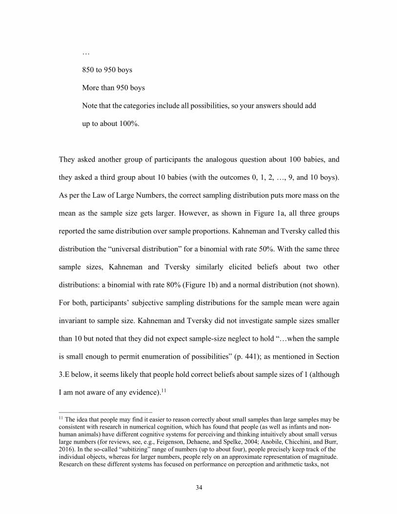
850 to 950 boys

More than 950 boys

Note that the categories include all possibilities, so your answers should add

up to about 100%.

They asked another group of participants the analogous question about 100 babies, and

they asked a third group about 10 babies (with the outcomes 0, 1, 2, …, 9, and 10 boys).

As per the Law of Large Numbers, the correct sampling distribution puts more mass on the

mean as the sample size gets larger. However, as shown in Figure 1a, all three groups

reported the same distribution over sample proportions. Kahneman and Tversky called this

distribution the “universal distribution” for a binomial with rate 50%. With the same three

sample sizes, Kahneman and Tversky similarly elicited beliefs about two other

distributions: a binomial with rate 80% (Figure 1b) and a normal distribution (not shown).

For both, participants’ subjective sampling distributions for the sample mean were again

invariant to sample size. Kahneman and Tversky did not investigate sample sizes smaller

than 10 but noted that they did not expect sample-size neglect to hold “…when the sample

is small enough to permit enumeration of possibilities” (p. 441); as mentioned in Section

3.E below, it seems likely that people hold correct beliefs about sample sizes of 1 (although

I am not aware of any evidence).11

11 The idea that people may find it easier to reason correctly about small samples than large samples may be consistent with research in numerical cognition, which has found that people (as well as infants and non-human animals) have different cognitive systems for perceiving and thinking intuitively about small versus large numbers (for reviews, see, e.g., Feigenson, Dehaene, and Spelke, 2004; Anobile, Chicchini, and Burr, 2016). In the so-called “subitizing” range of numbers (up to about four), people precisely keep track of the individual objects, whereas for larger numbers, people rely on an approximate representation of magnitude. Research on these different systems has focused on performance on perception and arithmetic tasks, not

35

Despite pre-dating Tversky and Koehler (1994) by two decades, Kahneman and

Tversky (1972a) anticipated the potentially confounding effect of partition dependence.

They emphasized that “in contrast [to previous studies], subjects evaluate[d] the same

number of categories for all sample sizes” (p. 441). Indeed, according to the model of

partition dependence in equations (3.1) and (3.3), if the bins are held constant and if the

function g is assumed to be the same across sample sizes, then the insensitivity of the

reported-belief distributions to sample size implies that the root-belief distributions are also

the same across sample sizes.

There have been several replications and extensions of Kahneman and Tversky’s

elicitation of full sampling-distributions beliefs. Recently, Benjamin, Moore, and Rabin

(2018) elicited subjective sampling distributions about flips of a fair coin. They asked about

samples of size 10, 1000, and 1 million, each with the same 11-bin partition used by

Kahneman and Tversky. Despite incentivizing participants’ responses and eliciting all

three distributions from each participant, they found identical subjective sampling

distributions across the three sample sizes. In an early replication, Olson (1976) reinforced

Kahneman and Tversky’s concern about the potentially confounding influence of partition

dependence. Olson asked different groups of undergraduates to provide the sampling

distribution for the percentage of boys born in regions with 100 and 1,000 babies born per

day. When he used the same 11-bin partition as Kahneman and Tversky, he found identical

distributions like they did. However, Olson also elicited the distributions using other

partitions. For example, he asked another group of participants about the 100-baby

distribution, but this time using an 11-bin partition with the outcomes <46, 46, 47, …, 53,

probabilistic reasoning. One might conjecture that intuitions for probabilistic reasoning are built in to the small-number system but not the large-number system.

36

54, and >54 boys. He found that the probabilities that participants assigned to these 11 bins

were similar to those they assigned when the 11 bins corresponded to Kahneman and

Tversky’s partition. For instance, the median participant assigned only a slightly higher

probability to the lowest category in the new partition—3% for <46 boys—than to the

lowest category in Kahneman and Tversky’s partition—1% for 0-5 boys—even though the

true probability is much higher in the first case (18% versus roughly 0%).

Kahneman and Tversky interpreted sample-size neglect as showing that “The

notion that sampling variance decreases in proportion to sample size is apparently not part

of man’s repertoire of intuitions” (p. 444). Sedlmeier and Gigerenzer (1997) proposed a

more specific hypothesis: when asked about the distribution of means across samples,

people instead give an answer about the distribution of outcomes within a sample. Among

several pieces of evidence, the most telling comes from Sedlmeier (1994, Study 2, as

described by Sedlmeier and Gigerenzer), who replicated and extended Kahneman and

Tversky’s elicitation of sampling-distribution beliefs about a normal distribution. Similar

to prior work, Sedlmeier’s experimental participants constructed distributions for the mean

height of Israeli soldiers for sample sizes of 20 and 200—and, as in prior findings, the two

distributions were identical. Another group of participants constructed distributions for

height (as opposed to mean height) for these two sample sizes, i.e., distributions of heights

for 20 soldiers and for 200 soldiers. These two distributions looked extremely similar, as

they should, but they were also extremely similar to the distributions of mean height

produced by the other participants, suggesting that the participants had no intuition that the

two tasks were different.

37

Kahneman and Tversky reported further evidence of sample-size neglect from other

questions that did not require participants to construct a distribution and are arguably less

subject to confounding from partition dependence. For example, they asked whether a

hospital with 45 births per day or one with 15 births per day would record more days with

at least 60% of births being boys, or whether the two hospitals would have “About the

same” number of days. Although the correct answer is the smaller hospital, more than half

the participants chose “About the same,” and roughly equal numbers chose the larger and

smaller hospitals. This finding again points to people not understanding that the variance

of the sampling distribution shrinks with sample size. It has been replicated in several

dozen studies involving many variants of the judgment problem (for a review, see Lem,

Dooren, Gillard, and Verschaffel, 2011).

Notwithstanding the evidence described above, people do seem to have two

intuitions about the role of sample size, both originally identified by Bar-Hillel (1979).

First, when asked directly, people expect the mean from a larger sample to be closer to the

population mean. In a particularly clean demonstration, Well, Pollatsek, and Boyce (1990,

Experiment 2) asked about the average height of the men registering at two conscription

registration centers, one in which 25 men register per day and one in which 100 register

per day, and told participants that the national average height in the population of men is 5

feet 9 inches. Similar to the hospital problem, one group of undergraduates was asked

which center has more days when the average height exceeds 6 feet, and only 8% gave the

correct answer of the smaller center. However, another group was asked which center will

measure an average height closer to the national average on a particular day, and a third

group was asked which will have more days when the average height is between 5 feet 6

38

inches and 6 feet (a 6-inch interval around the national average). In these latter two

conditions, respectively 59% and 56% gave the correct answer. Well, Pollatsek, and Boyce

concluded that although people have some basic understanding of the Law of Large

Numbers, they do not understand its implications for the variance of the sampling

distribution. I further discuss people’s intuition that large samples are more likely to have

means close to the population mean in Section 3.D.

Relatedly, Evans and Dusoir (1977, Experiment 2) hypothesized that when the

question itself makes the logic clear to people, they can understand that extreme outcomes

are less likely in large samples. Several studies have found evidence that has been

interpreted as supporting this hypothesis (e.g., Bar-Hillel, 1979; Pelham and Neter, 1995,

Study 1). For example, Bar-Hillel (1979) posed a version of the hospital problem with 15

and 5 births per day and asked which hospital recorded more days on which all the babies

born were boys. In this problem, over half the participants correctly chose the smaller

hospital and only a quarter chose “About the same.” Bar-Hillel (1982) reported further

evidence from versions of the problem that asked different groups of participants which

hospital had more days in which the percentage of births being boys was over 60%, over

70%, over 80%, and 100%. She found that as the percentage became more extreme, more

participants gave the correct answer. This seems to contradict the evidence from eliciting

the full sampling distribution, discussed above, that people construct the same “universal

distribution” regardless of sample size, even in the tails of the distribution, but constructing

the distribution is arguably a more difficult task that does not give clues as to the correct

intuition.

39

Second, people have an incorrect intuition that what matters for getting a sample

mean close to the population mean is the ratio of the sample size to the population size,

rather than the absolute sample size. Mathematically, as long as a sample is drawn with

replacement, only the absolute sample size matters (and even if a sample is drawn without

replacement, the ratio matters very little as long as the ratio is small). In one of Bar-Hillel’s

(1979, Experiment 4) studies, she described two urns, one containing 10 beads and one

containing 100 beads, each with the same unknown proportions of red and green beads.

She asked participants whether they would be more likely to correctly guess the majority

color if they took 9 draws with replacement from the small urn or 15 draws with

replacement from the large urn. 72 out of 110 participants erroneously chose the smaller

number of draws from the small urn, presumably because it has a higher ratio of draws to

urn size. Evans and Bradshaw (1986) also found evidence that experimental participants

incorrectly believe they can draw stronger inferences when the ratio of sample size to

population size is larger. I am not aware of any work that has explored the psychology

underlying this intuition or its broader implications.

Benjamin, Rabin, and Raymond (2016) proposed a model to capture sample-size

neglect. They called the bias that generates sample-size neglect Non-Belief in the Law of

Large Numbers (NBLLN). In the model, signals are drawn i.i.d. from a binomial

distribution whose rate of a signals is . The agent, however, forms beliefs as if any

particular sample is generated by a two-step process: (i) a “subjective rate” is drawn

from some distribution that has mean and full support on [0,1], called the “subjective-

rate distribution”; and then (ii) the signals for the sample are drawn i.i.d. from a binomial

distribution whose rate is . This model directly generates sample-size neglect in large

θ

β

θ

β

40

samples: if were the actual rate, the proportion of a signals in a large sample would be

(by the Law of Large Numbers). Therefore, in a large sample, the probability density

that the agent assigns to any proportion of signals (say, 60% of babies are boys) is equal to

the probability density that the subjective-rate distribution assigns to equaling that value.

In other words, as the sample size gets large, the agent’s subjective sampling distribution

for the mean converges to the subjective-rate distribution. Thus, in the model, the

subjective-rate distribution is the “universal distribution” that the agent believes

characterizes any large enough sample—and Kahneman and Tversky’s evidence indicates

that a sample size of 10 is already “large enough.” For a sample size of one, the model

implies that the agent has correct sampling-distribution beliefs. For any sample size larger

than one, the agent’s subjective sampling distribution is flatter than the correct distribution

(due to the randomness of ), and the agent believes that tail events are more likely than

they are.

Benjamin, Rabin, and Raymond used the model as a tool to explore the implications

of sample-size neglect in a number of settings, including risky decision making. A number

of implications follow from the agent’s belief that the tails of the sampling distribution—

such as all a’s or all b’s—are more likely than they are. To give some examples, if winning

a lottery requires matching all numbers, and matching each number has probability , then

the agent will overestimate his chance of winning and be too willing to play. If success at

a job fair requires getting at least one job offer, and getting any job offer has probability

, then the agent will overestimate his chance of getting no offers and will undervalue

attending. If each of many stocks has positive expected value and earns money with

β

β

β

β

θ

θ

41

independent probability , then the agent overestimates the variance of payoffs in a

diversified portfolio and hence will undervalue diversification.

Similarly, the model predicts that people will undervalue a repeated, positive-

expected-value gamble. Benartzi and Thaler (1999) reported evidence from several studies

on attitudes toward repeated gambles and long-term investing that they interpreted as

consistent with sample-size neglect (related evidence is reported in Keren and Wagenaar,

1987, Keren, 1991, and Redelmeier and Tversky, 1992). For example, when undergraduate

experimental participants were asked the probability of a net loss after 150 repetitions of a

90%/10% bet to gain $0.10/lose $0.50, participants’ mean estimate was 24%—a dramatic

overestimate relative to the correct probability of 0.3%. When actually offered this repeated

gamble, only 49% accepted it. Yet 90% said they would accept a single-play bet that had

the true distribution of money outcomes implied by the repeated bet, suggesting that they

would have accepted the repeated bet if they had correctly understood the distribution of

outcomes.

NBLLN also has implications for how people draw inferences. I will defer

discussion of these implications until Section 5.A.

3.C. Sampling-Distribution-Tails Diminishing Sensitivity

As discussed above, NBLLN implies sample-size neglect: for large enough sample

sizes, people’s subjective sampling distribution is determined by a “universal distribution”

that is invariant to sample size. This in turn implies that for large sample sizes, the tails of

the subjective sampling distribution are fat relative to the true tails. There is also some

evidence that the tails of the “universal distribution” are flat relative to the true tails.

θ

42

NBLLN implies some flatness, but the amount of flatness is greater than can be explained

by Benjamin, Rabin, and Raymond’s (2016) model of NBLLN. Benjamin, Rabin, and

Raymond (2016, Appendix C) conjectured that this excess flatness is due to another bias,

which they called sampling-distribution-tails diminishing sensitivity (SDTDS): people

think of unlikely outcomes as similar to each other.

Apparent flatness of the tails is evident in Figure 1b, which shows Kahneman and

Tversky’s survey data for the binomial with rate 0.8. In the true distribution for a sample

size of 100, as one goes from 45-55% to 35-45% to 25-35% heads, the probability declines

at an exponential rate, from 0.73 to 0.14 to 0.001. In contrast, the median participant’s

estimate declines much more slowly, from 0.22 to 0.15 to 0.10. Much of the other evidence

from experimental participants’ constructed sampling distributions also features flat tails

(e.g., Wheeler and Beach, 1968; Peterson, DuCharme, and Edwards, 1968, Study 2;

Teigen, 1974b). All of this evidence, however, is confounded by partition dependence,

which would compress participants’ estimates relative to their root beliefs.

In experiments designed to identify sampling-distribution beliefs separately from

compression, Benjamin, Moore, and Rabin (2018) found evidence of flat tails for sample

sizes of 1000 and 1 million. For example, experimental participants’ sampling distribution

for 1000 coin flips was elicited using the 5-bin partition: 0-487, 488-496, 497-503, 504-

512, and 513-1000 heads. This partition was chosen because each bin has roughly equal

true probability. Consequently, as discussed in Section 3.A, the deviation of beliefs away

from equality indicates the direction of bias in root beliefs net of partition dependence.

Mean beliefs had a “W” shape, overweighting the middle bin and extreme-tail bins but

underweighting the intermediate-tail bins: mean beliefs were 26%, 13%, 21%, 14%, and

43

27%, compared with the true probabilities of 21.5%, 19.8%, 16.5%, 19.8%, and 21.5%,

respectively. The combination of overweighting extreme tails but underweighting

intermediate tails implies that the tail beliefs are too flat.

3.D. Overweighting the Mean and the Fallacy of Large Numbers

As discussed in Section 3.B, when people construct sampling distributions for

samples of different sizes, they do not assign higher probability to the population mean in

the larger sample size. Yet, as also discussed there, there is much evidence that when people

are asked directly, they do have an intuition that when the sample is larger, the sample

mean is likely to be closer to the population mean. Moreover, from experiments that control

for confounding from partition dependence, there is some evidence that when people

construct sampling distributions, they assign too much weight to the population mean. For

example (as mentioned in Section 3.C), in five-bin elicitations of beliefs about samples of

1000 and 1 million coin flips, Benjamin, Moore, and Rabin (2018) found that relative to

the true probabilities, experimental participants overweighted both the extreme-tail bins

and the middle bin. Olson (1976) also found evidence that points to overweighting the

mean, net of partition dependence. For instance (as also discussed in Section 3.C), some of

his experimental participants constructed sampling distributions for how often a 100-baby

sample would have different percentages of boys. Among participants where the middle

bin in an 11-bin partition was 45-55 boys, participants’ median estimate was 40% (the true

probability is 68%). Among a different group of participants where the middle bin in an

11-bin partition was exactly 50 boys, participants’ median estimate was actually slightly

higher: 45% (the true probability is 8%).

44

Further evidence comes from Klos, Weber, and Weber (2005), who asked their

experimental participants a set of questions about four repeated gambles. For example, one

gamble was a 50-50 chance to win 200 euros or lose 100 euros. When participants were

asked about the standard deviation of payoffs or about probability of a loss, it was clear

that participants assigned too much probability mass to the tails, replicating Benartzi and

Thaler’s (1999) evidence of NBLLN. But participants were also asked the probability that

the outcome would fall within +/- 100 euros of the expected value in 5 or 50 repetitions of

the gamble. While the true probability is 21% for 5 repetitions and 7% for 50 repetitions,

participants’ mean estimates were dramatically too high: 47% and 58%.

This evidence is consistent with people having some correct Law of Large Numbers

intuition. Yet the overestimation of the probability that the sample mean will match the

population mean is more suggestive of the Law of Small Numbers (LSN) bias discussed in

Section 2.A. The (incorrect) LSN intuition is that extreme sample realizations tend to be

counteracted by additional signals (as opposed to the correct Law of Large Numbers

intuition, which is that the effect of extreme sample realizations on the sample mean is

diluted by additional signals). However, the LSN bias by itself does not explain why, in

Klos, Weber, and Weber’s experiment, participants’ estimates—contrary to the true

probabilities—are higher for 50 repetitions than for 5 repetitions. Klos, Weber, and

Weber’s comparison between 50 and 5 repetitions was motivated as a test of Paul

Samuelson’s (1963) hypothesis that people suffer from a “fallacy of large numbers.”

Samuelson had hypothesized that people have a specific misunderstanding of the Law of

Large Numbers: while the correct idea is that for fixed , asε > 0 p 1NΣ i=1N si −θ < ε

⎛⎝⎜

⎞⎠⎟→1

45

, he argued people incorrectly think that . In words, the Law

of Large Numbers states that the mean of the signals in the sample becomes arbitrarily

close to the population rate. The fallacy states incorrectly that the sum total of the signals

becomes arbitrarily close to its expected value.12

Psychologically, the fallacy of large numbers is closely related to the LSN: it is the

belief that the GF is stronger in larger samples. More precisely, the GF is the belief that

below-average realizations and above-average realizations tend to cancel out in any

sample, whereas the fallacy of large numbers states that below-average and above-average

realizations will perfectly cancel out in an arbitrarily large sample.

The fallacy-of-large-numbers hypothesis is plausible but logically contradicts

sample-size neglect / NBLLN: if people’s sampling-distribution beliefs are pinned down

by a “universal distribution” over proportions regardless of sample size, then they would

believe that the probability of the outcome ending up in any fixed interval converges

to zero as . Because of this contradiction, Benartzi and Thaler (1999) interpreted

their evidence of NBLLN (see Section 3.B) as casting doubt on the fallacy-of-large-

numbers hypothesis. But this internal inconsistency between biases could be a case where

which bias occurs depends on which question a person is asked; for related discussion, see

Sections 3.B, 3.F, and 10.B. Another possibility is that the fallacy-of-large-numbers

12 For readers unfamiliar with the “fallacy of large numbers” hypothesis, some orientation regarding its history may be helpful. Samuelson noted that an MIT colleague said he would turn down a single gamble like the one studied by Klos, Weber, and Weber (a 50-50 chance to win 200 euros or lose 100 euros) but accept many repetitions of the gamble. Samuelson argued that his colleague’s willingness to accept many repetitions was a mistake, and he proposed the fallacy of large numbers to explain the supposed mistake. Benartzi and Thaler (1999) documented behavior like that of Samuelson’s colleague in surveys and experiments (see Section 3.B), but they argued that people’s error is turning down the single gamble (due to loss aversion; see Chapter XXX (by O’Donoghue and Sprenger) in this Handbook), rather than accepting the repeated gamble. Moreover, as noted below, Benartzi and Thaler interpreted their evidence of NBLLN as evidence against the fallacy-of-large-numbers hypothesis.

N→∞ p Σ i=1N si − Nθ < ε( )→1

Σ i=1N si

N→∞

46

hypothesis is not the correct explanation of Klos, Weber, and Weber’s evidence. I am not

aware of other tests of the hypothesis.

Overall, my reading of the data is that NBLLN coexists with a sampling-

distribution bias of overweighting the mean, which may be due to the LSN. At this point,

there is not enough evidence for a confident judgment about whether there is also a fallacy-

of-large-numbers bias.

3.E. Sampling-Distribution Beliefs for Small Samples

All of the evidence discussed so far has been from sample sizes of at least 10. There

are two papers that elicited subjective sampling distributions for smaller sample sizes.

Wheeler and Beach (1968) elicited two binomial sampling distributions, with rates

and 0.8 and both with a sample size of N = 8. They found that their participants’

distributions were too flat.13 Peterson, DuCharme, and Edwards (1968, Study 2) elicited

nine binomial sampling distributions, with the three rates = 0.6, 0.7, and 0.8 and the three

sample sizes N = 3, 5, and 8. They found that participants’ sampling distributions were

roughly correct for N = 3 but were flatter than the correct distributions for N = 5 and

especially for N = 8. In all cases, beliefs were elicited using a partition that binned each

possible outcome separately (e.g., 0, 1, 2, and 3). Thus, the evidence from both papers

confounds the root-belief distributions with compression due to partition dependence,

which would also flatten reported-belief distributions. Taking compression into account,

13 Wheeler and Beach’s study had a sequence of stages, and the sampling distributions were elicited three times over the course of the study. In between, the participants observed realized samples, made bets about which distribution each sample was drawn from, and then received feedback about whether they were correct (see Section 4.A for further discussion). While participants’ sampling distributions were too flat at the beginning of the experiment (prior to any feedback), by the end of the experiment the distributions were too peaked.

θ = 0.6

θ

47

Peterson et al.’s results may suggest that people’s root-belief distributions are too peaked

for sample sizes of 3, rather than too flat.

Using an elicitation designed to control for compression, Benjamin, Moore, and

Rabin (2018) studied beliefs about samples of 10 coin flips and found no evidence that

participants’ root-belief distribution was too flat. Specifically, they elicited beliefs using

the 5-bin partition 0-3, 4, 5, 6, and 7-10 heads, which is the partition that comes closest to

equal true probabilities in each bin (17%, 21%, 25%, 21%, and 17%). According to the

model of compression effects in Section 2.C, with such a partition, the direction of bias of

reported beliefs also indicates the direction of bias of root beliefs. In both their convenience

sample of adults and their sample of undergraduates, Benjamin et al. found that mean

beliefs were approximately correct (18%, 22%, 28%, 18%, and 14% for the adults and

16%, 18%, 32%, 18%, and 16% for the students), except with some overweighting of the

middle bin. These results suggest that, for sample sizes of 10, people’s root-belief

distribution is roughly correct or too peaked.

Putting the scant evidence together, it suggests that for sample sizes between one

and 10, people’s root-belief sampling distributions may be too peaked. I am not aware of

any evidence regarding beliefs about samples of size one, probably because such an

elicitation would be weird for experimental participants. It seems likely that such beliefs

are correct: people would believe that the probability of an a signal in a single draw when

the rate is known to be is equal to .

θ θ

48

3.F. Summary and Comparison of Sequence Beliefs Versus Sampling-Distribution

Beliefs

Psychologists have identified two main biases in people’s beliefs about sequences

of random events: the GF and the hot-hand bias, both of which may be due to the LSN

(Sections 2.A and 2.B). The LSN also appears to influence people’s beliefs about sampling

distributions, causing them to assign too much probability to the possibility that the sample

mean will be close to the population rate (Section 3.D).

People’s sampling-distribution beliefs, however, are also influenced by other

biases: partition dependence (Section 3.A), NBLLN (Section 3.B), and perhaps SDTDS

(Section 3.C). Summarizing all of the evidence from Section 3 and focusing on what can

be inferred about root beliefs: for “small” sample sizes (say, smaller than 10), people think

the sampling distribution is too peaked, while for non-small sample sizes, people think the

sampling distribution has tails that are too fat and too flat but also that put too much weight

at the mean. Most of this evidence can be rationalized by LSN dominating at the small

sample sizes and by LSN, NBLLN, and SDTDS jointly influencing beliefs at the larger

sample sizes.

People’s sampling-distribution beliefs are internally inconsistent due to partition

dependence. Even if we put this aside by focusing on root beliefs, people’s sampling-

distribution beliefs are inconsistent with their sequence beliefs because several biases (such

as NBLLN and SDTDS) influence sampling-distribution but not sequence beliefs.

In some direct tests in which sampling-distribution beliefs and sequence beliefs

were elicited from the same experimental participants, Benjamin, Moore, and Rabin (2018)

reported evidence of such inconsistency (suggestive evidence of such inconsistency was

49

also reported by Teigen, 1974a). For example, experimental participants’ root beliefs about

the distribution of the number of heads out of 10 coin flips are roughly correct, as

mentioned in Section 3.E. This would imply that people think 9 heads out of 10 flips is 10

times more likely than 10 heads out of 10 flips. But, as per the GF, they believe that heads

is roughly half as likely as tails following a streak of 9 heads. And since, given the GF,

participants surely think that the nine other ways to get 9 heads out of 10 are at least as

likely as HHHHHHHHHT, their sequence beliefs imply that 9 out of 10 heads should be

at least 20 times more likely than 10 out of 10 heads.

This internal inconsistency means that people’s beliefs about a random sample will

depend on whether they are thinking about the sequence of signals or the distribution

generated by that sequence. Economic models have generally not drawn this distinction,

and I am not aware of work that studies when people think about sequences versus

distributions, but these will be important issues to work out. I briefly discuss some of the

related modeling challenges in Section 10.B.

50

Section 4. Evidence on Belief Updating

Belief updating is the revision of beliefs upon receipt of new information. The core

component of the neoclassical theory of probabilistic beliefs is the assumption that people

update beliefs according to Bayes’ Theorem. This section is about the evidence on

deviations from Bayesian updating. The review in this section aims to be comprehensive,

except that I focus on settings where people are motivated only to be accurate; I defer

discussion of settings where people also have preferences over which state of the world is

true until Section 9.

For simplicity, I will describe Bayesian updating (and deviations from it) in the

case where there are two states of the world, A and B. Denote the agent’s prior beliefs,

before observing new signals, by and . Bayes’ Theorem prescribes how to

update the prior beliefs to posterior beliefs after observing some set of signals, S:

(4.1)

(4.2)

where is the likelihood of observing S in state A, and is the likelihood

of observing S in state B.14 It is often useful to write Bayes’ Theorem in its posterior-odds

form, obtained by dividing equation (4.1) by equation (4.2):

14 Bayes’ Theorem is an immediate consequence of the definition of conditional probability,

. Using this definition for the first and last equalities:

, and is derived analogously.

p(A) p(B)

p(AɈS) = p(S Ɉ A)p(A)p(S Ɉ A)p(A)+ p(S Ɉ B)p(B)

p(B ɈS) = p(S Ɉ B)p(B)p(S Ɉ A)p(A)+ p(S Ɉ B)p(B)

p(S Ɉ A) p(S Ɉ B)

p(X ɈY ) ≡p(X∩Y )p(Y ) p(AɈS) =

p(A∩S)p(S)

=p(S∩A)

p(S∩A)+p(S∩B)=

p(S Ɉ A)p(A)p(S Ɉ A)p(A)+ p(S Ɉ B)p(B)

p(B ɈS)

51

(4.3)

This equation states that the posterior odds of state A to state B, , is equal to the

likelihood ratio, , times the prior odds, .

Much of the evidence on how people update their beliefs comes from what I will

refer to as updating problems. In an updating problem, experimental participants are given

priors and a set of signals from which the likelihoods could be calculated, and then their

posterior beliefs are elicited. To illustrate this type of problem, Edwards (1968, p. 20-21)

gave a hypothetical example:

Imagine two urns filled with millions of poker chips. In the first urn, 70

percent of the chips are red and 30 percent are blue. In the second urn, 70

percent are blue and 30 percent are red. Suppose one of the urns is chosen

randomly and a dozen chips are drawn from it: eight red chips and four blue

chips. What are the chances that the chips came from the urn with mostly

red chips? (Give your answer as a percentage.)

Here, the two states are A = {mostly red urn} and B = {mostly blue urn}, the prior

probabilities are , and assuming that the chips are drawn with

replacement (as in most of the experiments), the likelihoods can be calculated using the

binomial distribution.

p(AɈS)p(B ɈS)

= p(S Ɉ A)p(A)p(S Ɉ B)p(B)

p(AɈS)p(B ɈS)

p(S Ɉ A)p(S Ɉ B)

p(A)p(B)

p(A) = p(B) = 0.5

52

Biased updating can be identified by comparing people’s posteriors with the correct

posteriors. For example, Edwards reports that in his example, the intuitive answer for most

people is roughly 70% or 80%. The correct answer is calculated by plugging the

likelihoods, and ,

and the priors into equation (4.1). Doing so yields a correct answer of 97%—much larger

than most people anticipate! In this example, people underinfer, meaning that they infer

less from the evidence than they should.

This section reviews the evidence on such deviations of people’s posterior beliefs

from normatively correct posterior beliefs in updating problems. Although Edwards’s

example is hypothetical, there are many dozens of experiments that have been conducted

in which poker chips are actually drawn out of urns in front of the participants (or balls are

drawn out of bookbags, etc.). These are often called bookbag-and-poker-chip experiments.

Most of the evidence reviewed in this section comes from bookbag-and-poker-chip

experiments.

Most of these experiments were published in the psychology literature during 1964-

1973 and are unfamiliar to economists.15 Some historical context helps to understand why.

The pioneers in studying deviations from Bayesian updating were Ward Edwards, a

psychologist, and his student, Larry Phillips (Edwards and Phillips, 1964; Phillips and

Edwards, 1966). Edwards had written two important early reviews of behavioral decision

research (1954, 1961b) and a seminal paper introducing psychologists to Bayesian statistics

15 This literature also included a number of experiments on deviations from the Bayesian model of demand for information (e.g., Green, Halbert, and Minas, 1964; Edwards and Slovic, 1965). For economists, this work is also unfamiliar but relevant. I do not review it here.

p(S Ɉ A) = 128

⎛

⎝⎜⎞

⎠⎟(0.7)8(0.3)4 = 0.231 p(S Ɉ B) = 12

8⎛

⎝⎜⎞

⎠⎟(0.3)8(0.7)4 = 0.008

53

that remains a classic among statisticians (Edwards, Lindman, and Savage, 1963). It was

thus natural for him and other psychologists at the time to ask how people’s actual updating

compares to Bayes’ Theorem. The bookbag-and-poker-chip paradigm was the workhorse

in this active literature.

As discussed in Section 7 of this Chapter, Daniel Kahneman and Amos Tversky’s

persuasive “heuristics and biases” research program, beginning with Tversky and

Kahneman (1971) and Kahneman and Tversky (1972a), redirected psychologists’ attention

toward understanding the psychological processes underlying belief judgments. In the

meantime, Edwards’s interests shifted toward designing computer programs to aid people

in applying Bayes’ Theorem to their priors and likelihood judgments (Edwards, 1968).

After 1973, the psychology literature on biased belief updating became dominated by the

sort of hypothetical updating scenarios that Kahneman and Tversky employed (which more

closely resembled real-world situations than Edwards’s abstract environments did).

Economists were influenced by Kahneman and Tversky’s work. When David

Grether (1980) conducted the first economics experiments on belief updating, he framed it

as testing whether Kahneman and Tversky’s representativeness heuristic describes

people’s beliefs when people are financially motivated and experienced, and he did not

mention the earlier psychology literature at all.16 Yet instead of posing hypothetical

judgment scenarios via surveys as Kahneman and Tversky had done, Grether adopted the

bookbag-and-poker-chip paradigm as his experimental methodology in order to make the

random process transparent to participants and to better control the information that

16 In personal correspondence, David Grether told me that early drafts of his paper had referenced the bookbag-and-poker-chip literature in psychology (as he had done in his review paper, Grether (1978)), but his recollection is that a referee asked him to remove those references.

54

participants might use to fill in unspecified scenario details. Subsequent economics

experiments have continued to use the bookbag-and-poker-chip paradigm but have built

on the findings of the precursor economics experiments rather than on the much earlier

psychology experiments.

This section draws on both the earlier psychology literature and the more recent

experiments in economics and psychology. To help organize this large body of evidence, I

will supplement the literature review with a meta-analysis. To organize the findings,

throughout the section I summarize a sequence of “stylized facts” that I will refer back to

in subsequent sections of this chapter.

4.A. Conceptual Framework

To organize the evidence on belief-updating biases, I will use the following

reduced-form model introduced by Grether (1980)17:

(4.4)

, (4.5)

17 To be more precise, equations (4.4)-(4.6) are the implicit model underlying Grether’s specification. Grether introduced the empirical regression specification in equation (4.15) below (both with and without the indicator term), which can be derived by taking the logarithm of equation (4.6) below and adding a constant term and an error term. Many subsequent economics papers have followed Grether (1980) in estimating this equation or its sequential-sample analog, equation (4.21) below, introduced by Grether (1992). For an alternative organizing framework, see Epstein, Noor, and Sandroni (2008).

π (AɈS) = p(S Ɉ A)c p(A)d

p(S Ɉ A)c p(A)d + p(S Ɉ B)c p(B)d

π (B ɈS) = p(S Ɉ B)c p(B)d

p(S Ɉ A)c p(A)d + p(S Ɉ B)c p(B)d

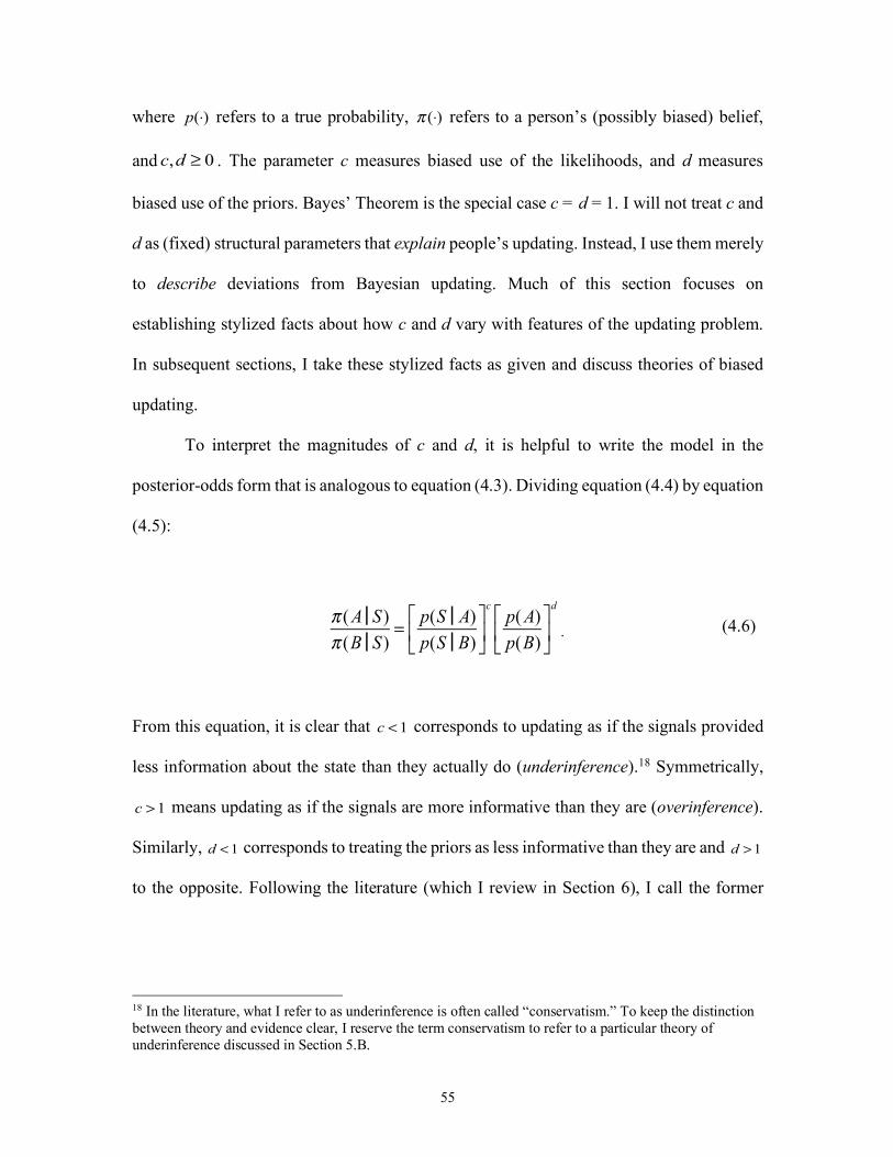
55

where refers to a true probability, refers to a person’s (possibly biased) belief,

and . The parameter c measures biased use of the likelihoods, and d measures

biased use of the priors. Bayes’ Theorem is the special case c = d = 1. I will not treat c and

d as (fixed) structural parameters that explain people’s updating. Instead, I use them merely

to describe deviations from Bayesian updating. Much of this section focuses on

establishing stylized facts about how c and d vary with features of the updating problem.

In subsequent sections, I take these stylized facts as given and discuss theories of biased

updating.

To interpret the magnitudes of c and d, it is helpful to write the model in the

posterior-odds form that is analogous to equation (4.3). Dividing equation (4.4) by equation

(4.5):

. (4.6)

From this equation, it is clear that corresponds to updating as if the signals provided

less information about the state than they actually do (underinference).18 Symmetrically,

means updating as if the signals are more informative than they are (overinference).

Similarly, corresponds to treating the priors as less informative than they are and

to the opposite. Following the literature (which I review in Section 6), I call the former

18 In the literature, what I refer to as underinference is often called “conservatism.” To keep the distinction between theory and evidence clear, I reserve the term conservatism to refer to a particular theory of underinference discussed in Section 5.B.

p(⋅) π (⋅)

c,d ≥ 0

π (AɈS)π (B ɈS)

= p(S Ɉ A)p(S Ɉ B)

⎡

⎣⎢

⎤

⎦⎥

cp(A)p(B)

⎡

⎣⎢

⎤

⎦⎥

d

c <1

c >1

d <1 d >1

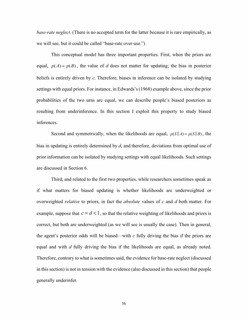
56

base-rate neglect. (There is no accepted term for the latter because it is rare empirically, as

we will see, but it could be called “base-rate over-use.”)

This conceptual model has three important properties. First, when the priors are

equal, , the value of d does not matter for updating; the bias in posterior

beliefs is entirely driven by c. Therefore, biases in inference can be isolated by studying

settings with equal priors. For instance, in Edwards’s (1968) example above, since the prior

probabilities of the two urns are equal, we can describe people’s biased posteriors as

resulting from underinference. In this section I exploit this property to study biased

inferences.

Second and symmetrically, when the likelihoods are equal, , the

bias in updating is entirely determined by d, and therefore, deviations from optimal use of

prior information can be isolated by studying settings with equal likelihoods. Such settings

are discussed in Section 6.

Third, and related to the first two properties, while researchers sometimes speak as

if what matters for biased updating is whether likelihoods are underweighted or

overweighted relative to priors, in fact the absolute values of c and d both matter. For

example, suppose that , so that the relative weighting of likelihoods and priors is

correct, but both are underweighted (as we will see is usually the case). Then in general,

the agent’s posterior odds will be biased—with c fully driving the bias if the priors are

equal and with d fully driving the bias if the likelihoods are equal, as already noted.

Therefore, contrary to what is sometimes said, the evidence for base-rate neglect (discussed

in this section) is not in tension with the evidence (also discussed in this section) that people

generally underinfer.

p(A) = p(B)

p(S Ɉ A) = p(S Ɉ B)

c = d <1

57

The c and d parameters can be estimated from updating from simultaneous samples,

in which people update in response to a one-shot sample of signals, or from updating from

sequential samples, in which people update dynamically as additional signals are observed.

Because the latter is more complex, I begin with evidence from simultaneous samples in

Section 4.B and then turn to evidence from sequential samples in Section 4.C.19

4.B. Evidence from Simultaneous Samples

Here I will review a set of stylized facts regarding biased inferences and biased use

of priors that have emerged from simultaneous-sample experiments. I will both describe

the results from specific experiments as well as report a meta-analysis intended to

summarize the evidence from the literature as a whole. The meta-analysis extends the

earlier meta-analysis reported by Benjamin, Rabin, and Raymond (2016, Appendix D) with

additional data20 and new analyses.

The vast majority of bookbag-and-poker-chip experiments focus on a particular

class of updating problems: there are two states of the world, A and B; there are two signals,

a and b; and the signals are drawn i.i.d., with probability of an a signal in state A and

in state B. Participants are given the prior probabilities, and then they either observe a

sequence of signals, such as aabab, or they are just told the total number of realized a and

19 Recently, Augenblick and Rabin (2018) showed how a researcher can infer the directions of deviation of c and d from one based on observing how a person’s probabilistic beliefs change in response to signals, even when the signals are not observed by the researcher. I am not aware of any empirical work yet that has estimated the biases using this approach. 20 Specifically, here I add data from 6 new papers to the meta-analysis sample, bringing the total number of papers to 16. In addition, I conduct a new meta-analysis of 5 sequential-sample papers by combining sequential observations from 3 of the papers included in the earlier analysis with sequential-sample data from 2 new papers. The sequential-sample meta-analysis is discussed in Section 4.C below.

θ A

θB

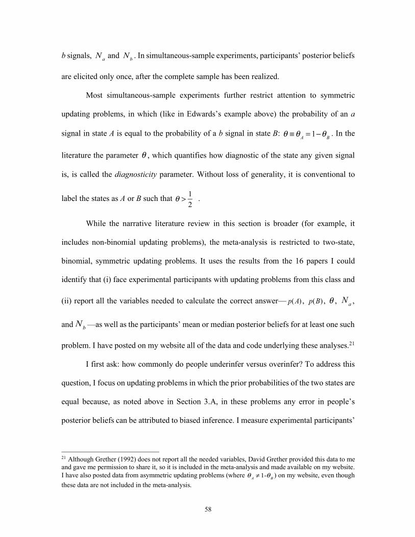
58

b signals, and . In simultaneous-sample experiments, participants’ posterior beliefs

are elicited only once, after the complete sample has been realized.

Most simultaneous-sample experiments further restrict attention to symmetric

updating problems, in which (like in Edwards’s example above) the probability of an a

signal in state A is equal to the probability of a b signal in state B: . In the

literature the parameter , which quantifies how diagnostic of the state any given signal

is, is called the diagnosticity parameter. Without loss of generality, it is conventional to

label the states as A or B such that .

While the narrative literature review in this section is broader (for example, it

includes non-binomial updating problems), the meta-analysis is restricted to two-state,

binomial, symmetric updating problems. It uses the results from the 16 papers I could

identify that (i) face experimental participants with updating problems from this class and

(ii) report all the variables needed to calculate the correct answer— , , , ,

and —as well as the participants’ mean or median posterior beliefs for at least one such

problem. I have posted on my website all of the data and code underlying these analyses.21

I first ask: how commonly do people underinfer versus overinfer? To address this

question, I focus on updating problems in which the prior probabilities of the two states are

equal because, as noted above in Section 3.A, in these problems any error in people’s

posterior beliefs can be attributed to biased inference. I measure experimental participants’

21 Although Grether (1992) does not report all the needed variables, David Grether provided this data to me and gave me permission to share it, so it is included in the meta-analysis and made available on my website. I have also posted data from asymmetric updating problems (where ) on my website, even though these data are not included in the meta-analysis.

Na Nb

θ ≡ θ A = 1−θB

θ

θ > 12

p(A) p(B) θ Na

Nb

θ A ≠ 1-θB

59

posterior beliefs using log posterior odds, . This quantity is positive if

participants believe that state A is more likely and negative if they believe that state B is

more likely.

For each of the inference problems included in the meta-analysis, Figure 2 Panel A

plots participants’ log posterior odds on the y-axis against the correct log posterior odds,

, on the x-axis. The identity line (the dashed line in the figure) corresponds to

Bayesian inference. To interpret the regression slope (the solid line), note that taking the

logarithm of equation (4.6), participants’ log posterior odds can be written

, (4.7)

and taking the logarithm of equation (4.3), the correct log posterior odds are

. (4.8)

In both equations, the prior-odds term vanishes because the updating problems are

restricted to those with equal priors:

, (4.9)

ln π (AɈS)π (B ɈS)

⎛⎝⎜

⎞⎠⎟

ln p(AɈS)p(B ɈS)

⎛⎝⎜

⎞⎠⎟

ln π (AɈS)π (B ɈS)

⎛⎝⎜

⎞⎠⎟= c ln p(S Ɉ A)

p(S Ɉ B)⎛⎝⎜

⎞⎠⎟+ d ln p(A)

p(B)⎛⎝⎜

⎞⎠⎟

ln p(AɈS)p(B ɈS)

⎛⎝⎜

⎞⎠⎟= ln p(S Ɉ A)

p(S Ɉ B)⎛⎝⎜

⎞⎠⎟+ ln p(A)

p(B)⎛⎝⎜

⎞⎠⎟

ln π (AɈS)π (B ɈS)

⎛⎝⎜

⎞⎠⎟= c ln p(S Ɉ A)

p(S Ɉ B)⎛⎝⎜

⎞⎠⎟

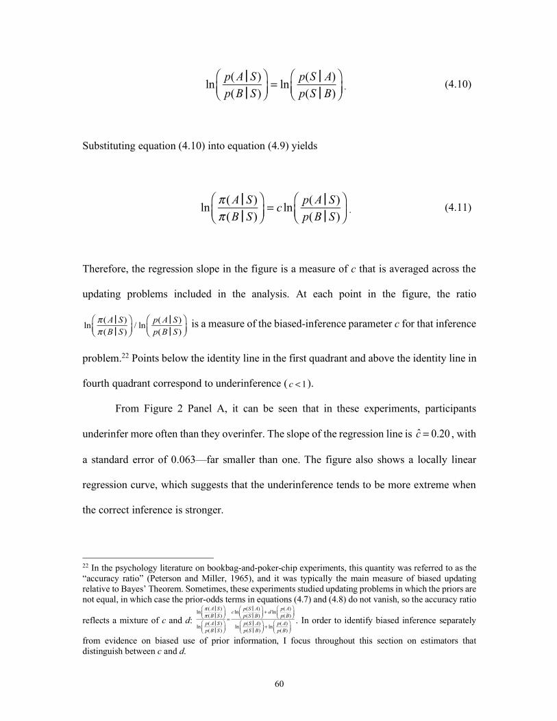
60

. (4.10)

Substituting equation (4.10) into equation (4.9) yields

. (4.11)

Therefore, the regression slope in the figure is a measure of c that is averaged across the

updating problems included in the analysis. At each point in the figure, the ratio

is a measure of the biased-inference parameter c for that inference

problem.22 Points below the identity line in the first quadrant and above the identity line in

fourth quadrant correspond to underinference ( ).

From Figure 2 Panel A, it can be seen that in these experiments, participants

underinfer more often than they overinfer. The slope of the regression line is , with

a standard error of 0.063—far smaller than one. The figure also shows a locally linear

regression curve, which suggests that the underinference tends to be more extreme when

the correct inference is stronger.

22 In the psychology literature on bookbag-and-poker-chip experiments, this quantity was referred to as the “accuracy ratio” (Peterson and Miller, 1965), and it was typically the main measure of biased updating relative to Bayes’ Theorem. Sometimes, these experiments studied updating problems in which the priors are not equal, in which case the prior-odds terms in equations (4.7) and (4.8) do not vanish, so the accuracy ratio

reflects a mixture of c and d: . In order to identify biased inference separately

from evidence on biased use of prior information, I focus throughout this section on estimators that distinguish between c and d.

ln p(AɈS)p(B ɈS)

⎛⎝⎜

⎞⎠⎟= ln p(S Ɉ A)

p(S Ɉ B)⎛⎝⎜

⎞⎠⎟

ln π (AɈS)π (B ɈS)

⎛⎝⎜

⎞⎠⎟= c ln p(AɈS)

p(B ɈS)⎛⎝⎜

⎞⎠⎟

ln π (AɈS)π (B ɈS)

⎛⎝⎜

⎞⎠⎟/ ln p(AɈS)

p(B ɈS)⎛⎝⎜

⎞⎠⎟

c <1

c = 0.20

ln π (AɈS)π (B ɈS)

⎛⎝⎜

⎞⎠⎟

ln p(AɈS)p(B ɈS)

⎛⎝⎜

⎞⎠⎟

=c ln p(S Ɉ A)

p(S Ɉ B)⎛⎝⎜

⎞⎠⎟+ d ln p(A)

p(B)⎛⎝⎜

⎞⎠⎟

ln p(S Ɉ A)p(S Ɉ B)

⎛⎝⎜

⎞⎠⎟+ ln p(A)

p(B)⎛⎝⎜

⎞⎠⎟

61

The first column of Table 2 Panel A shows the linear regression results displayed

in Figure 2 Panel A. In the second column, the analysis is restricted to updating problems

from incentivized experiments. In those experiments, the estimate is , with a

standard error of 0.028, indicating somewhat less but still substantial underinference on

average and less noisy behavior.

In experiments with binomial signals that did not meet all the criteria for inclusion

in the meta-analysis, underinference has also been the general finding.23 In addition,

underinference has been the usual finding in experiments where, instead of the signals

being binomial, the signals are multinomial.24 When a signal is drawn from a normal

distribution, underinference has occurred when the signal realization is far from its

expected value in either state, and otherwise, nearly Bayesian inference or overinference

has occurred.25

To summarize:

Stylized Fact 1. Underinference is by far the dominant direction of bias.

This conclusion may be surprising since, in our personal experiences, many of us observe

people jumping to conclusions. After discussing the rest of the evidence and various

theories, Section 10.A returns to this apparent tension and discusses potential

reconciliations. Section 5 discusses the leading theories for explaining underinference.

23 For example, Chinnis and Peterson (1968), Peterson and Swensson (1968), Sanders (1968), De Swart (1972a), De Swart (1972b), and Antoniou, Harrison, Lau, and Read (2015). 24 For example, Beach (1968), Phillips, Hays, and Edwards (1966, Study 1), Dale (1968), Martin (1969), Martin and Gettys (1969), Shanteau (1972), and Chapman (1973). 25 Nearly Bayesian inference was found by DuCharme and Peterson (1968, Studies 1 and 2) and DuCharme (1970, Studies 1 and 2), while overinference was found by Gustafson, Shukla, Delbecq, and Walster (1973).

c = 0.38

62

I next ask: how is underinference related to sample size, ? As a

measure of the bias in inference, I will use the updating-problem-specific estimate

discussed above, .

A number of papers have manipulated sample size while holding constant other

features of the inference problem and reported the results in such a way that the relationship

between N and can be seen. Every such paper has found that larger N is associated with

more underinference as measured by smaller .26

Turning to the meta-analysis sample, which includes studies that do not manipulate

N, Figure 3 Panel A plots the inference measure against N. The value of is mostly smaller

than one, as expected given that underinference is the predominant direction of bias. The

slope of the regression line is negative, indicating that is smaller at larger sample sizes.

A locally linear regression suggests that the relationship between underinference and

sample size is steeper at smaller sample sizes.

Stylized Fact 2. Underinference (as measured by ) is more severe the larger the sample

size.

Are inferences biased at a sample size of 1? While the regression line in Figure 3

Panel A suggests that there is underinference when N = 1, the value of the regression line

here relies largely on extrapolation from larger sample sizes. Focusing only on the 16

26 I have found nine such papers: Green, Halbert, and Robinson (1965), Pitz (1967), Peterson, DuCharme, and Edwards (1968, Study 2), Peterson and Swensson (1968), Sanders (1968), Kahneman and Tversky (1972a), Griffin and Tversky (1992, Study 1), Nelson, Bloomfield, Hales, and Libby (2001, Study 1), and Kraemer and Weber (2004).

N = Na + Nb

c

ln π (AɈS)π (B ɈS)

⎛⎝⎜

⎞⎠⎟/ ln p(AɈS)

p(B ɈS)⎛⎝⎜

⎞⎠⎟

c

c

c

c

c

63

updating problems with N = 1, the mean is 0.70 with a standard error of 0.057; restricted

to the 7 updating problems from incentivized experiments, the mean is 0.86 with a standard

error of 0.078. Thus, the data from the meta-analysis sample points to underinference from

a sample size of 1.27

Among experiments with binomial updating problems and a sample size of 1 that

did not meet all the criteria for inclusion in the meta-analysis, nearly all found substantial

underinference or slight underinference,28 with one exception (Robalo and Sayag, 2014).29

One experiment observed overinference in an experimental condition with asymmetric

rates that are close to each other (Peterson and Miller, 1965, , ). In an

experiment with a sample size of 1 in which the signal was drawn from a multinomial

distribution, Phillips, Hays, and Edwards (1966) found nearly Bayesian inference. As noted

above, when a single signal is drawn from a normal distribution, underinference has

occurred when the signal realization is far from its expected value in either state but not

otherwise.30

Thus, while there are exceptions (which may or may not be systematic), the

evidence from N = 1 samples can be summarized as generally finding underinference:

27 For sample sizes of 2, 3, 4, 5, and 6, the corresponding mean is 0.73 (SE = 0.07), 0.98 (SE = 0.10), 0.52 (SE = 0.08), 1.06 (SE = 0.09), and 0.67 (SE = 0.10), respectively. Thus, the broad impression is underinference across these small sample sizes, but we cannot reject overinference for sample sizes of 3 and 5. 28 Substantial underinference was found by Dave and Wolfe (2003) and Gettys and Manley (1968, Studies 1 and 2), whereas slight underinference was found by Chinnis and Peterson (1968), Peterson and Swensson (1968, Study 1), Kraemer and Weber (2004), Sasaki and Kawagoe (2007), and Ambuehl and Li (2018). 29 Robalo and Sayag (2014) studied a symmetric binomial updating problem with 60-40 priors. Their experimental participants did not have posteriors that are systematically less extreme than Bayesian posteriors. Depending on the degree of base-rate neglect, their evidence could be consistent with either Bayesian inference or overinference. 30 DuCharme and Peterson (1968, Studies 1 and 2), DuCharme (1970, Studies 1 and 2), and Gustafson, Shukla, Delbecq, and Walster (1973).

c

θ A = 0.6 θB = 0.4

c

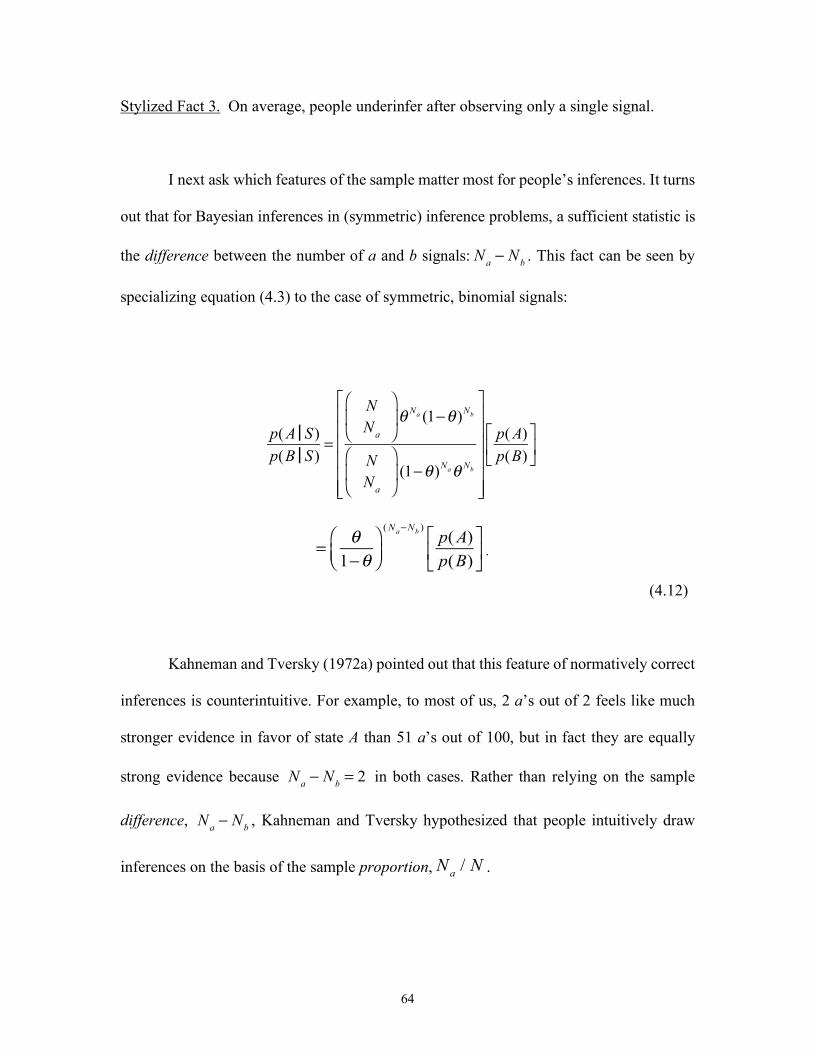
64

Stylized Fact 3. On average, people underinfer after observing only a single signal.

I next ask which features of the sample matter most for people’s inferences. It turns

out that for Bayesian inferences in (symmetric) inference problems, a sufficient statistic is

the difference between the number of a and b signals: . This fact can be seen by

specializing equation (4.3) to the case of symmetric, binomial signals:

.

(4.12)

Kahneman and Tversky (1972a) pointed out that this feature of normatively correct

inferences is counterintuitive. For example, to most of us, 2 a’s out of 2 feels like much

stronger evidence in favor of state A than 51 a’s out of 100, but in fact they are equally

strong evidence because in both cases. Rather than relying on the sample

difference, , Kahneman and Tversky hypothesized that people intuitively draw

inferences on the basis of the sample proportion, .

Na − Nb

p(AɈS)p(B ɈS)

=

NNa

⎛

⎝⎜

⎞

⎠⎟θ Na (1−θ )Nb

NNa

⎛

⎝⎜

⎞

⎠⎟ (1−θ )Naθ Nb

⎡

⎣

⎢⎢⎢⎢⎢⎢

⎤

⎦

⎥⎥⎥⎥⎥⎥

p(A)p(B)

⎡

⎣⎢

⎤

⎦⎥

= θ1−θ

⎛⎝⎜

⎞⎠⎟

(Na−Nb ) p(A)p(B)

⎡

⎣⎢

⎤

⎦⎥

Na − Nb = 2

Na − Nb

Na / N

65

Kahneman and Tversky tested this hypothesis in a set of ten hypothetical updating

problems. One of these problems31 was (p. 447):

Consider two very large decks of cards, denoted A and B. In deck A, 2/3 of

the cards are marked a, and 1/3 are marked b. In deck B, 1/3 of the cards

are marked a, and 2/3 are marked b. One of the decks has been selected by

chance, and 12 cards have been drawn at random from it, of which 8 are

marked a and 4 are marked b. What do you think the probability is that the

12 cards were drawn from deck A, that is, from the deck in which most of

the cards are marked a?

In this problem, which is similar to Edwards’s problem quoted above, the proportion of a

signals is 2/3, and the difference between the number of a and b signals is 4. Similarly, as

in Edwards’s problem, the median subject reported a belief of 70%, much weaker than the

correct posterior of 94%. Two other problems, each asked to a different group of subjects,

were the same except that the numbers of a and b signals were changed from 8 and 4 (in

the quoted problem above) to 4 and 2 in one problem and to 40 and 20 in the other. These

problems hold constant the proportion of a signals but, by manipulating the sample size,

change the true probabilities to 80% and 99.9999%, respectively. Yet, consistent with

Kahneman and Tversky’s hypothesis, the median subject’s reported belief was virtually

unaffected: 68% and 70%, respectively.

31 In the original statement of the problem, the cards were marked “X” and “O.” I’ve changed them to “a” and “b” for consistency of notation with the rest of this chapter. Moreover, while Kahneman and Tversky quote directly from their problem with , I instead describe their other set of problems, with , for greater comparability with Edwards’ illustrative problem above.

θ = 5 / 6 θ = 2 / 3

66

In other problems, Kahneman and Tversky varied the proportion but held constant

the difference and found that people reported a higher belief in state A when the proportion

of a signals was higher. Kahneman and Tversky’s finding that beliefs depend only on the

sample proportion is an extreme result32; other experiments in the literature (discussed

next) also find support for the hypothesis that people’s inferences are influenced by the

sample proportion, but they generally find that the difference between the number of a and

b signals also matters.

Evans and Dusoir (1977) also found that many people rely on sample proportion

over sample size (in a more complex experiment, Evans and Pollard (1982) reach the same

conclusion). They asked undergraduates to make pairwise judgments such as whether a

sample of coin flips with 8 heads and 2 tails provides stronger or weaker evidence of a

heads-biased coin than a sample of 70 heads and 30 tails. When sample proportion and

sample size considerations conflicted, as in this example, more than two-thirds of

participants endorsed the sample with the larger proportion as providing more evidence.

Griffin and Tversky (1992) quantified the relative roles of sample size and sample

proportions in driving people’s inferences. They posed twelve updating problems to each

32 Kahneman and Tversky’s results are also extreme in another way: they find that the median subject’s posterior belief is completely insensitive to the diagnosticity parameter . For example, in three updating problems identical to the those mentioned above but with instead of 2/3, the median subject’s posterior belief was 70% in all three cases. As discussed below, such complete insensitivity to " has not been observed in updating problems more generally. Why were Kahneman and Tversky’s results so extreme? A possible explanation is that the median subject was following a simple heuristic of setting their posterior belief roughly equal to the sample proportion . As Kahneman and Tversky pointed out, for all three sample proportions they investigated, the median subject’s posterior belief was very nearly equal to the sample proportion and was insensitive to both N and . Earlier, Beach, Wise, and Barclay (1970) proposed that people follow this heuristic (and cite Kriz (1967) as having proposed it even earlier). Beach, Wise, and Barclay found evidence consistent with this heuristic in simultaneous-sample updating problems but not sequential-sample updating problems. Marks and Clarkson (1972) found that roughly 2/5 of their experimental participants seemed to follow this heuristic. As discussed below, Griffin and Tversky (1992) found that their median participant’s posterior was somewhat sensitive to N and , which is inconsistent with the median participant reporting beliefs according to this heuristic.

θθ = 5 / 6

π (AɈNa ,Nb) Na / N

θ

θ

67

of their undergraduate participants, with equal priors for the two states and the diagnosticity

parameter fixed at . Across the twelve problems, the number of signals varied from 3

to 33, and the sample proportion varied from 0.53 (9 a’s out of 17) to 1 (3 a’s out of 3 and

5 out of 5). To assess how participants’ use of sample size and sample proportion deviated

from Bayesian inference, Griffin and Tversky estimated a regression equation that nests

Bayesian inference as a special case. I will derive this regression in four steps.

The starting point is the formula for Bayesian inference in symmetric binomial

problems, equation (4.12), when the priors are equal:

.

The first step is to obtain a linear equation by taking the double logarithm33:

.

33 Griffin and Tversky ensured that all of the terms in this equation are well defined by setting and

posing updating problems in which . In the meta-analysis data I analyze below, I guarantee

by labeling the states such that state A has the higher rate of a signals. However, does not hold for all of the observations. To include in the analysis the observations where , I exploit the symmetry of

the updating problem, switching and and replacing participants’ posterior odds in equation

(4.14) by . For example, if participant’s posterior odds were after observing a 4 b’s and 1 a, I enter it into the analysis as if the odds were 3 after having observed 4 a’s and 1 b. I drop the 25 observations for which in the simultaneous-sample experiments and 16 such observations in the sequential-sample experiments.

θ 35

p(AɈS)p(B ɈS)

= θ1−θ

⎛⎝⎜

⎞⎠⎟

(Na−Nb )

ln ln p(AɈS)p(B ɈS)

⎛⎝⎜

⎞⎠⎟

⎛⎝⎜

⎞⎠⎟= ln(Na − Nb)+ ln ln

θ1−θ

⎛⎝⎜

⎞⎠⎟

⎛⎝⎜

⎞⎠⎟

θ = 35> 12

Na > Nb θ > 12

Na > NbNa < Nb

Na Nbπ (AɈS)π (B ɈS)

π (B ɈS)π (AɈS)

13

Na = Nb

68

Second, to separate out the role of the sample proportion, the sample-difference term is

decomposed into the sum of a sample-proportion term and a sample-size term:

.

Third, this rule for Bayesian inference is generalized by allowing the coefficients to differ

from one, and a response-error term is added:

.

(4.13)

Finally, because did not vary across their updating problems, Griffin and Tversky

absorbed the term into the constant:

. (4.14)

The null hypothesis of Bayesian inference is . By estimating regression

equation (4.14), Griffin and Tversky tested whether the sample proportion and sample size

ln ln p(AɈS)p(B ɈS)

⎛⎝⎜

⎞⎠⎟

⎛⎝⎜

⎞⎠⎟= ln

Na − NbN

⎛⎝⎜

⎞⎠⎟+ ln(N )+ ln ln θ

1−θ⎛⎝⎜

⎞⎠⎟

⎛⎝⎜

⎞⎠⎟

ln ln π (AɈS)π (B ɈS)

⎛⎝⎜

⎞⎠⎟

⎛⎝⎜

⎞⎠⎟=α0 +α1 ln

Na − NbN

⎛⎝⎜

⎞⎠⎟+α 2 ln(N )+

α3 ln lnθ1−θ

⎛⎝⎜

⎞⎠⎟

⎛⎝⎜

⎞⎠⎟+ ε

θ

θ

α1 =α 2 = 1

69

are weighted as much as they should be according to Bayesian inference as well as how

they are weighted relative to each other.

Griffin and Tversky reported estimates of and ,

respectively.34 To interpret these results, note first that the hypothesis is rejected;

thus, experimental participants are not drawing inferences based on the difference between

the number of a signals and the number of b signals. Next, the results indicate that both

and are smaller than one, consistent with underinference on average (Stylized Fact 1),

and points to greater underinference from larger samples (Stylized Fact 2). Since

the hypothesis and is rejected, Griffin and Tversky’s results are less

extreme than Kahneman and Tversky’s (1972a): participants’ inferences are not entirely

driven by the sample proportion; they do take sample size into account to some extent.

Finally, the results indicate that , meaning that relative to (the correct) equal

weighting of sample proportion and sample size, sample proportion influences inferences

by more.

Griffin and Tversky’s regression can be replicated in the meta-analysis data.

Because this data has variation in , I estimate equation (4.13) rather than equation (4.14).

The first column of Table 3 Panel A shows the results. The estimates are consistent with

Griffin and Tversky’s reported estimates, not only qualitatively but even quantitatively: the

34 Specifically, Griffin and Tversky (p. 416) wrote: “For the median data, the observed regression weight for strength (.81) was almost 3 times larger than that for weight (.31).” However, when I estimate equation (4.14) using the median data reported in Griffin and Tversky, I find = 0.44 (SE = 0.115), = 1.02 (SE = 0.094), and = 0.17 (SE = 0.064). In personal communication with Dale Griffin, we were unable to recover how the regression in the paper differed from my regression. Regardless of which estimates are used, the main conclusions are the same.

α1 = 0.81 α 2 = 0.31

α1 =α 2

α1

α 2

α 2 <1

α1 = 1 α 2 = 0

α1 >α 2

θ

α1α 2

70

estimated coefficient on sample proportion, , is 0.85 with a standard error of 0.071, and

the estimated coefficient on sample size, , is 0.41 with a standard error of 0.049. (I

discuss the coefficient on the term below.) The third column of the table repeats the

analysis but restricted to incentivized experiments, and the results are similar. Thus, while

sample size matters to some extent, the sample proportion has a much greater impact on

participants’ inferences on average.

Stylized Fact 4. Rather than depending on the sample difference, , people’s

inferences are largely driven by the sample proportion, .

Beginning with Grether (1980), several papers have investigated the hypothesis that

the sample proportion has an especially large impact on inference when it equals the rate

of a signals in one of the states. Grether’s idea was that if the sample proportion equals

(say) , then participants can rely on the representativeness heuristic (discussed in

Section 7) in drawing an inference in favor of state A. Elaborating on this idea, Camerer

(1987) referred to the hypothesis that people draw stronger inferences when the sample

proportion exactly matches one of the rates as “exact representativeness.”

In Grether’s experiment, the prior probability of state A varied across conditions,

equaling 1/3, 1/2, or 2/3. The probability of an a signal was = 2/3 in state A and =

1/2 in state B. Experimental participants observed a set of N = 6 signals and guessed

whether the state was A or B. In some conditions, participants were paid a bonus for

guessing accurately. To analyze his data, Grether ran a regression corresponding to

α1

α 2

θ

Na − Nb

Na − NbN

θ A

θ A θB

71

equation (4.7) but with indicator variables for the observed sample proportion matching

the states’ rates:

.

(4.15)

Because participants reported a guess about the state rather than a posterior probability,

Grether estimated a logistic regression version of this equation, and thus the absolute

magnitudes of the coefficients are not straightforward to interpret. Across various

specifications and subsamples, his results generally indicated and , consistent

with exact representativeness. However, in two similar experiments conducted

subsequently, Grether (1992) found much more equivocal evidence.

Camerer (1987, 1990) aimed to test whether biased updating would survive in

markets. He conducted an experimental asset market, in which participants traded a state-

contingent asset. In each round of the experiment, participants observed a set of N = 3

signals before trading. The probability of an a signal was 2/3 in state A and 1/3 in state B.

Consistent with exact representativeness, he found that when the observed sample

contained 2 a’s and 1 b, the price of a state-contingent asset that pays off in state A was too

high, and when the observed sample contained 1 a and 2 b’s, the price of a state-contingent

asset that pays off in state B was too high.

ln π (AɈS)π (B ɈS)

⎛⎝⎜

⎞⎠⎟= β0 + β1 ln

p(S Ɉ A)p(S Ɉ B)

⎛⎝⎜

⎞⎠⎟+ β2 ln

p(A)p(B)

⎛⎝⎜

⎞⎠⎟

+β3INaN

= θ A⎧⎨⎩

⎫⎬⎭+ β4I

NaN

= θB⎧⎨⎩

⎫⎬⎭+η

β3 > 0 β4 < 0

72

To assess the evidence regarding “exact representativeness” more broadly in

bookbag-and-poker-chip experiments, I analyze the meta-analysis sample. Because this

sample has variation in N and and is restricted to updating problems with equal priors, I

estimate a version of equation (4.13) rather than equation (4.15). Specifically, Column 2

of Table 3 Panel A shows the results when I have included an indicator for the sample

proportion being equal to . (There is no indicator for the sample proportion being equal

to 1- because, as per footnote 33, all observations are coded such that and

.)

The coefficient on this indicator is 0.02, with a standard error of 0.086. The sign is

in accordance with what exact representativeness would predict, but the standard error is

much larger than the point estimate. Thus, I find little evidence for exact representativeness

in the meta-analysis sample, but the estimate is too noisy to draw strong conclusions.

Stylized Fact 5. While some experiments have found evidence of overinference, or less

underinference, when the observed sample proportion equals the rate in one of the states,

it has not been robustly seen across experiments.

As a final question about inference: how is underinference related to the

diagnosticity parameter, ? Almost every study35 that varies while holding constant

other features of the updating problem has found greater underinference (as measured by

35 Green, Halbert, and Robinson (1965), Peterson and Miller (1965), Sanders (1968), Peterson and Swensson (1968, Studies 1 and 2), Peterson, DuCharme, and Edwards (1968, Study 2), Beach, Wise, and Barclay (1970), Kahneman and Tversky (1972a), Donnell and DuCharme (1975). Vlek (1965) and Vlek and van der Heiden (1967) are cited in Slovic and Lichtenstein (1971) as also finding this result, but I have not been able to track down those papers.

θ

θ

θ θ > 12

Na > Nb

θ θ

c

73

) for further from ½, with the exceptions of Gettys and Manley (1968), who found no

relationship, and Shanteau (1972), who found the opposite in a multinomial-signal

experiment.

Turning to the meta-analysis data, Figure 4 Panel A plots against diagnosticity

. The slope of the regression line is -0.97 with a standard error of 0.27. The negative

slope indicates that as increases, there is more underinference on average, consistent

with what the individual studies have found.

To control for other factors that affect inferences and to examine whether

participants adequately account for (compared to Bayesian inference), I return to Table

3 Panel A and examine the coefficient on the diagnosticity term. As noted above, Bayesian

inference implies that the coefficient on should equal one. Instead, as seen

in Column 1, the coefficient estimate is 0.39 (standard error = 0.082). The estimate remains

similar, 0.52 (standard error = 0.097), when the sample is restricted to incentivized studies

(Column 3). The fact that this coefficient is in between zero and one indicates that subjects’

inferences take the different rates of a signals across states into account but less strongly

than they should.

In asymmetric updating problems (which are excluded from the meta-analysis),

there is some evidence that people overinfer when the rate of a signals in state A is similar

to the rate in state B. As mentioned above, Peterson and Miller (1965) found overinference

in inference problems with a single signal when the rates were = (0.6,0.43), but

they found underinference when the rates were further apart: = (0.83,0.17),

= (0.71,0.2), and = (0.67,0.33). Griffin and Tversky (1992, Study 3)

θ

c

θ

θ

θ

ln ln θ1−θ

⎛⎝⎜

⎞⎠⎟

⎛⎝⎜

⎞⎠⎟

(θ A,θB )

(θ A,θB )

(θ A,θB ) (θ A,θB )

74

posed a set of updating problems in which the number of a signals is 7, 8, 9, or 10. When

the rates were far apart, = (0.6,0.25), their experimental participants

underinferred: the median posterior beliefs that the state is A were .60, .70, .80, and .90,

respectively, whereas a Bayesian’s posteriors would be .95, .98, .998, and .999. In contrast,

when the rates were close together, = (0.6,0.5), the participants overinferred, with

median posterior beliefs .55, .66, .75, and .85, respectively, compared to a Bayesian’s

posteriors of .54, .64, .72, and .80.36 Grether (1992, Study 2) also found overinference in

asymmetric updating problems with = (0.67,0.5). Recently, in simultaneous-

sample updating problems with a single signal, Ambuehl and Li (2018) also found

underinference when and are far apart and overinference when they are close

together.

Stylized Fact 6. Underinference (as measured by ) is more severe the larger is the

diagnosticity parameter . In asymmetric inference problems, people may overinfer when

the rates and are close together.

36 Griffin and Tversky’s (1992, Study 3) evidence may also be related to a hypothesis, proposed by Vlek (1965), that people underinfer by more when an event occurs that is unlikely in both states. In a test of this hypothesis, Beach (1968) ran a bookbag-and-poker-chip experiment with multinomial signals: the letters A-F written on the back of a card. Cards were drawn from one of two decks, a red deck and a green deck, which had different proportions of the letters. Different groups of participants faced decks with the same likelihood ratios for the letters but different probabilities. For example, for one group, the probability of an F card was 0.03 for the red deck and 0.06 for the green deck, and for another group, 0.16 and 0.32. Holding the likelihood ratio fixed, Beach found greater underinference when the probabilities were smaller, consistent with Vlek’s hypothesis. Slovic and Lichtenstein (1971) reported that Vlek (1965) and Vlek and van der Heijden (1967) found similar results, but I have been unable to obtain those papers.

(θ A,θB )

(θ A,θB )

(θ A,θB )

θ A θB

c

θ

θ A θB

75

To conclude the summary of evidence from simultaneous-updating experiments, I

turn to biased use of priors. Five bookbag-and-poker-chip experiments that manipulated

the priors found that people under-use prior information relative to what is prescribed by

Bayes’ Theorem, and two found that people over-use prior information.37

To examine the evidence across studies, I now add into the meta-analysis sample

the updating problems with unequal priors. Whereas we had focused on problems with

equal priors in order to isolate biased inference, we cannot follow the analogous strategy

here of focusing on problems with equal likelihoods because there is little evidence from

such problems, and the results require more nuanced discussion; I defer discussion of that

evidence to Section 6. Therefore, in order to identify biased use of priors, I will need to

control for biased inferences.

To do so, I exploit the fact that we previously estimated biased inferences in

regression equation (4.13). The fitted values from that regression tell us what people’s

posterior odds would be in an updating problem with equal priors. Here, I will treat the

fitted values as telling us what people’s (biased) subjective likelihood ratio would be,

before it is combined with the prior odds. That is, we replace equation (4.6) by38

, (4.16)

37 Those that found under-use are Green, Halbert, and Robinson (1965), Bar-Hillel (1980), Griffin and Tversky (1992, Study 2), Grether (1992, Study 3), and Holt and Smith (2009), while those that found over-use are Peterson and Miller (1965) and Grether (1992, Study 2). 38 Alternatively, we could consider directly estimating equation (4.6), but I do not do so because it is misspecified if treated as a “structural” model: as discussed above, the results from estimating equation (4.13) tell us that the exponent c depends on sample size, sample proportion, and diagnosticity in the updating problem.

π (AɈS)π (B ɈS)

= π (S Ɉ A)π (S Ɉ B)

p(A)p(B)

⎡

⎣⎢

⎤

⎦⎥

d

76

where is a person’s subjective likelihood ratio, and for any given updating problem,

we use equation (4.13) to obtain an estimate of the logarithm of this subjective likelihood

ratio, .39 Next, we take the logarithm of equation (4.16) and isolate the prior

ratio on the right side:

. (4.17)

Figure 5 plots the left-hand side of equation (4.17) against the right-hand side. If

experimental participants correctly use prior odds, then d = 1, so the points should fall

along the identity line (the dashed line). Instead, the slope of the regression line (the solid

line) is less than one, indicating under-use of prior odds.

For more formal evidence, I estimate the regression equation:

. (4.18)

39 There is a nuance: the predicted value from equation (4.13) is an estimator for , but for

equation (4.17), what is needed is an estimate of . Simply exponentiating the estimate

is not a consistent estimator for due to Jensen’s inequality. I therefore generate

an estimate of by calculating , where and is the estimated

variance of the residual from equation (4.13). This estimator is consistent under the assumption that

is normally distributed.

π (S Ɉ A)π (S Ɉ B)

ln π (S Ɉ A)π (S Ɉ B)

⎛⎝⎜

⎞⎠⎟

!

ln π (AɈS)π (B ɈS)

⎛⎝⎜

⎞⎠⎟− ln π (S Ɉ A)

π (S Ɉ B)⎛⎝⎜

⎞⎠⎟

!= d ln p(A)

p(B)⎛⎝⎜

⎞⎠⎟

ln π (AɈS)π (B ɈS)

⎛⎝⎜

⎞⎠⎟− ln π (S Ɉ A)

π (S Ɉ B)⎛⎝⎜

⎞⎠⎟

!= γ 0 +γ 1 ln

p(A)p(B)

⎛⎝⎜

⎞⎠⎟+ζ

ln ln π (AɈS)π (B ɈS)

⎛⎝⎜

⎞⎠⎟

⎛⎝⎜

⎞⎠⎟

ln π (AɈS)π (B ɈS)

⎛⎝⎜

⎞⎠⎟

ln ln π (AɈS)π (B ɈS)

⎛⎝⎜

⎞⎠⎟

⎛⎝⎜

⎞⎠⎟

!ln π (AɈS)

π (B ɈS)⎛⎝⎜

⎞⎠⎟

ln π (AɈS)π (B ɈS)

⎛⎝⎜

⎞⎠⎟

eµ+12σ 2

µ = ln ln π (AɈS)π (B ɈS)

⎛⎝⎜

⎞⎠⎟

⎛⎝⎜

⎞⎠⎟

!σ 2

ln π (AɈS)π (B ɈS)

⎛⎝⎜

⎞⎠⎟

77

The results are shown in Table 4. The first column represents the regression illustrated in

Figure 5, while the second column restricts the data to experiments with unequal priors,

which is the subset of the data that identifies . As expected, the estimate of d, , is

essentially the same in both columns: 0.60 with a standard error of 0.066. This estimate of

d is substantially smaller than one, indicating that on average people under-use prior

information.

The third column of Table 4 re-runs the analysis from column 1, this time restricted

to incentivized experiments. In this case, the estimate of d is 0.43 with a standard error of

0.086, indicating even more extreme under-use of priors. Thus, both the evidence from

individual papers and the evidence from the meta-analysis point rather strongly to under-

use of prior information.

Stylized Fact 7. People exhibit base-rate neglect.

While the experiments discussed in Section 6 have been the focus of the literature on base-

rate neglect, Stylized Fact 7 shows that the evidence for base-rate neglect extends to

bookbag-and-poker-chip experiments.40

40 Few papers have addressed the question of whether giving people feedback leads to more accurate updating, but what evidence there is suggests only limited impact. Specifically, two papers have studied the effect of telling experimental participants the correct posterior probabilities after each updating problem. Martin and Gettys (1969) compared the effect of doing so with the effect of merely telling them the true state. The group that received posterior-probability feedback underinferred by less than the group that received true-state feedback, but over 200 trials, there was no detectable learning in either group, except possibly very early on. Donnell and DuCharme (1975) found that telling experimental participants the correct posterior probabilities after each of 60 updating problems eliminated their underinference, with almost all of the learning occurring in the first 10 trials. However, when participants were then faced with a new updating problem for which naïve participants tend to infer correctly, they overinferred. Donnell and

γ 1 γ 1!

78

4.C. Evidence from Sequential Samples

Up until now, I have focused on bookbag-and-poker-chip experiments in which the

sample was presented simultaneously. A number of bookbag-and-poker-chip experiments,

however, have been sequential-sample experiments: participants observe a sample

sequentially and report updated beliefs after each new signal (or set of signals) is observed.

I now turn to the evidence from these experiments.

An initial conceptual question—which matters for how the data should be

analyzed—is how people “group” signals. In the terminology of Benjamin, Rabin, and

Raymond (2016, Appendix A), who provide formal definitions, one hypothesis is that

people are acceptive: they group together signals that are presented to them together, and

they treat sets of signals presented separately as distinct samples. For example, suppose

two independent signals are observed sequentially. If people are acceptive, then they would

update their beliefs after each signal, with their updated beliefs after the first signal

becoming their priors when updating in response to the next signal. Another leading

hypothesis is that people are pooling: at any point in time, people pool all the signals they

have received up until that point and update from their initial priors using the pooled

sample.

For a Bayesian updater, the grouping of the signals is irrelevant. Continuing with

the example of two independent signals, suppose that a Bayesian is acceptive and hence

updates after each signal. Using equation (4.3), her posterior odds after the first signal are

DuCharme concluded that the feedback had caused participants to report more extreme beliefs but not to become better at drawing inferences.

79

,

and her posterior odds after the second signal are

If instead, she updates after the second signal by pooling both signals and updating from

her original priors, then her posterior odds after the second signal are

,

which are the same as the posterior odds from updating sequentially.

For a biased updater, however, grouping matters (see Cripps, 2018, for related

discussion). Using equation (4.6), if the agent is acceptive, then her posterior odds after the

first signal are

,

p(AɈ s1)p(B Ɉ s1)

=p(s1 Ɉ A)p(s1 Ɉ B)

p(A)p(B)

p(AɈ s1,s2 )p(B Ɉ s1,s2 )

=p(s2 Ɉ A)p(s2 Ɉ B)

p(AɈ s1)p(B Ɉ s1)

=p(s2 Ɉ A)p(s2 Ɉ B)

p(s1 Ɉ A)p(s1 Ɉ B)

p(A)p(B)

⎛

⎝⎜⎞

⎠⎟

=p(s1,s2 Ɉ A)p(s1,s2 Ɉ B)

p(A)p(B)

.

p(AɈ s1,s2 )p(B Ɉ s1,s2 )

=p(s1,s2 Ɉ A)p(s1,s2 Ɉ B)

p(A)p(B)

π (AɈ s1)π (B Ɉ s1)

=p(s1 Ɉ A)p(s1 Ɉ B)

⎡

⎣⎢

⎤

⎦⎥

c(1)p(A)p(B)

⎡

⎣⎢

⎤

⎦⎥

d

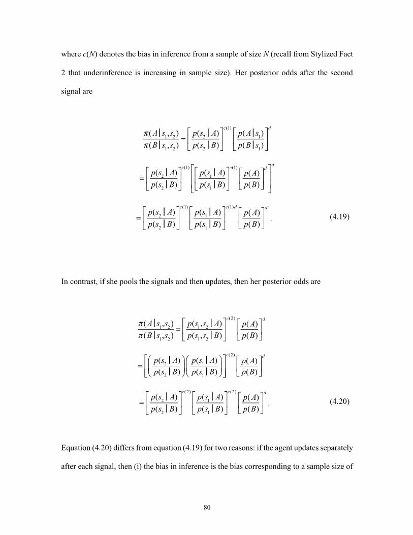
80

where c(N) denotes the bias in inference from a sample of size N (recall from Stylized Fact

2 that underinference is increasing in sample size). Her posterior odds after the second

signal are

. (4.19)

In contrast, if she pools the signals and then updates, then her posterior odds are

. (4.20)

Equation (4.20) differs from equation (4.19) for two reasons: if the agent updates separately

after each signal, then (i) the bias in inference is the bias corresponding to a sample size of

π (AɈ s1,s2 )π (B Ɉ s1,s2 )

=p(s2 Ɉ A)p(s2 Ɉ B)

⎡

⎣⎢

⎤

⎦⎥

c(1)p(AɈ s1)p(B Ɉ s1)

⎡

⎣⎢

⎤

⎦⎥

d

=p(s2 Ɉ A)p(s2 Ɉ B)

⎡

⎣⎢

⎤

⎦⎥

c(1)p(s1 Ɉ A)p(s1 Ɉ B)

⎡

⎣⎢

⎤

⎦⎥

c(1)p(A)p(B)

⎡

⎣⎢

⎤

⎦⎥

d⎡

⎣⎢⎢

⎤

⎦⎥⎥

d

=p(s2 Ɉ A)p(s2 Ɉ B)

⎡

⎣⎢

⎤

⎦⎥

c(1)p(s1 Ɉ A)p(s1 Ɉ B)

⎡

⎣⎢

⎤

⎦⎥

c(1)dp(A)p(B)

⎡

⎣⎢

⎤

⎦⎥

d2

π (AɈ s1,s2 )π (B Ɉ s1,s2 )

=p(s1,s2 Ɉ A)p(s1,s2 Ɉ B)

⎡

⎣⎢

⎤

⎦⎥

c(2)p(A)p(B)

⎡

⎣⎢

⎤

⎦⎥

d

=p(s2 Ɉ A)p(s2 Ɉ B)

⎛

⎝⎜⎞

⎠⎟p(s1 Ɉ A)p(s1 Ɉ B)

⎛

⎝⎜⎞

⎠⎟⎡

⎣⎢⎢

⎤

⎦⎥⎥

c(2)p(A)p(B)

⎡

⎣⎢

⎤

⎦⎥

d

=p(s2 Ɉ A)p(s2 Ɉ B)

⎡

⎣⎢

⎤

⎦⎥

c(2)p(s1 Ɉ A)p(s1 Ɉ B)

⎡

⎣⎢

⎤

⎦⎥

c(2)p(A)p(B)

⎡

⎣⎢

⎤

⎦⎥

d

81

1 rather than 2, and (ii) the information from the first signal is incorporated into the agent’s

prior when the second signal is processed, and so her biased use of priors affects how the

first signal enters into her final posterior. These differences can matter not only for the

analysis of experimental data, but also for the implications of biased updating in real-world

environments. For further discussion of the implications of (i) and (ii), see Sections 5.A

and 6, respectively.

Only two papers have explicitly tested experimentally between different grouping

hypotheses, and both find evidence against pooling. Pooling predicts that people’s posterior

beliefs should not depend on how signals are presented. In incentivized updating problems,

Kraemer and Weber (2004) found that mean beliefs of experimental participants presented

with a sample of 3 a signals and 2 b signals differed marginally from those of experimental

participants who were instead shown the same signals as two separate samples, one with 3

a’s and 0 b’s and one with 0 a’s and 2 b’s. Kraemer and Weber similarly found a difference

in posteriors when participants were presented with a single sample of 13 a’s and 12 b’s,

as opposed to a sequence of two samples, 13 a’s and 0 b’s and then 0 a’s and 12 b’s. Shu

and Wu (2003, Study 3) found that participants who observed 10 signals one at a time

reported a different posterior belief than participants who observed the same 10 signals two

at a time or five at a time.

Although less clean, comparisons between participants’ posteriors in simultaneous-

sample versus sequential-sample experiments also bear on the pooling hypothesis. Holding

constant other features of the updating problems, pooling predicts no differences in

participants’ posteriors. Sanders (1968) found less extreme posterior odds in sequential-

82

sample updating problems, while Beach, Wise, and Barclay (1970) found more extreme

posterior odds.

To obtain a more systematic comparison, I extended the meta-analysis sample to

incorporate updating problems in which participants were asked to report posteriors after

each signal in a sequence. As before, I restrict the sample to problems with equal (initial)

priors. Figures 2-4 and Tables 2-3 each have a Panel B, which repeats exactly the analysis

from Panel A but applied to these sequential-sample updating problems.

The figures and tables suggest that the same qualitative conclusions from the

simultaneous-sample experiments carry over to the sequential-sample experiments: on

average, participants’ final posteriors are less extreme when updating from larger final

sample sizes and more diagnostic rates. These qualitative conclusions also hold in every

individual sequential-sample experiment that manipulated sample size N or diagnosticity

.41

The pooling hypothesis, however, predicts that the results should be the same

quantitatively, but differences between the sequential-sample and simultaneous-sample

results are apparent in all the figures and tables. Table 3 Panel B provides another piece of

evidence against the pooling hypothesis: the estimated constant term is statistically

distinguishable from zero, which suggests that regression equation (4.13) is misspecified

for the sequential-sample updating problems. Across sequential-sample and simultaneous-

sample experiments with multinomial signals that held constant the final samples observed

by participants, Labella and Koehler (2004) found that participants had final posteriors that

41 For sample size, the experiments are Phillips, Hays, and Edwards (1966), Peterson and Swensson (1968), Sanders (1968), and Kraemer and Weber (2004); for diagnosticity, Phillips and Edwards (1966, Study 1 and 3), Pitz, Downing, and Reinhold (1967), Peterson and Swensson (1968), Sanders (1968), Chinnis and Peterson (1968), and Beach, Wise, and Barclay (1970).

θ

83

differed in several ways, which is again inconsistent with the pooling hypothesis. While

the evidence is not overwhelming, taken all together it casts substantial doubt on pooling.

Stylized Fact 8. In sequential-sample updating problems, people do not “pool” the signals

(i.e., update as if they had observed a single, simultaneous sample).

Therefore, I tentatively conclude that people are acceptive, updating after each set of

signals they observe—with the caveat that this conclusion has not been interrogated

empirically.

Given that people underinfer (Stylized Fact 1) and under-use priors (Stylized Fact

7), one would expect to see that the final posterior odds in sequential-sample experiments

are less extreme than Bayesian posterior odds. Indeed, essentially all sequential-sample

experiments that I am aware of have found final posterior odds that are less extreme than

Bayesian.42 This is also true on average for the meta-analysis sample, as shown in Figure

2 Panel B and Table 2 Panel B.

The quantitative differences between Panels A and B of the figures and tables are

difficult to interpret directly. If people are not pooling (Stylized Fact 8), then even if the

initial prior odds put equal weight on the two states, people’s subsequent prior odds in

general will not. Consequently, their posterior odds at the end of a sequential sample reflect

the effects of both biased inference and biased use of the priors.

42 The papers for which this is true are Peterson, Ulehla, Miller, Bourne, and Stilson (1965), Peterson, Schneider, and Miller (1965), Phillips and Edwards (1966), Phillips, Hays, and Edwards (1966), Beach (1968), Chinnis and Peterson (1968), Dale (1968), Peterson and Swensson (1968), Sanders (1968), Beach, Wise, and Barclay (1970), Edenborough (1975), Dave and Wolfe (2003), Kraemer and Weber (2004), and Sasaki and Kawagoe (2007). The one, partial exception is Strub (1969), who finds that while it is true for naïve experimental participants, participants with extensive training update Bayesianly.

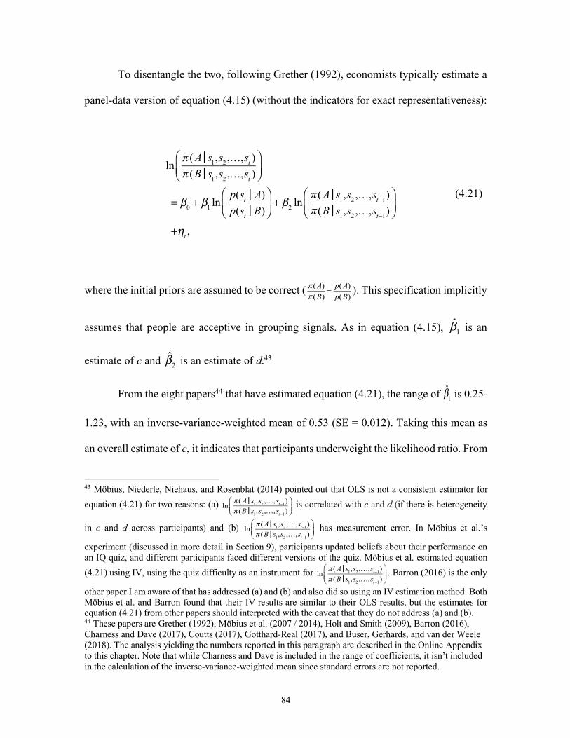
84

To disentangle the two, following Grether (1992), economists typically estimate a

panel-data version of equation (4.15) (without the indicators for exact representativeness):

(4.21)

where the initial priors are assumed to be correct ( ). This specification implicitly

assumes that people are acceptive in grouping signals. As in equation (4.15), is an

estimate of c and is an estimate of d.43

From the eight papers44 that have estimated equation (4.21), the range of is 0.25-

1.23, with an inverse-variance-weighted mean of 0.53 (SE = 0.012). Taking this mean as

an overall estimate of c, it indicates that participants underweight the likelihood ratio. From

43 Möbius, Niederle, Niehaus, and Rosenblat (2014) pointed out that OLS is not a consistent estimator for equation (4.21) for two reasons: (a) is correlated with c and d (if there is heterogeneity

in c and d across participants) and (b) has measurement error. In Möbius et al.’s

experiment (discussed in more detail in Section 9), participants updated beliefs about their performance on an IQ quiz, and different participants faced different versions of the quiz. Möbius et al. estimated equation (4.21) using IV, using the quiz difficulty as an instrument for . Barron (2016) is the only

other paper I am aware of that has addressed (a) and (b) and also did so using an IV estimation method. Both Möbius et al. and Barron found that their IV results are similar to their OLS results, but the estimates for equation (4.21) from other papers should interpreted with the caveat that they do not address (a) and (b). 44 These papers are Grether (1992), Möbius et al. (2007 / 2014), Holt and Smith (2009), Barron (2016), Charness and Dave (2017), Coutts (2017), Gotthard-Real (2017), and Buser, Gerhards, and van der Weele (2018). The analysis yielding the numbers reported in this paragraph are described in the Online Appendix to this chapter. Note that while Charness and Dave is included in the range of coefficients, it isn’t included in the calculation of the inverse-variance-weighted mean since standard errors are not reported.

lnπ (AɈ s1,s2 ,…,st )π (B Ɉ s1,s2 ,…,st )

⎛

⎝⎜⎞

⎠⎟

= β0 + β1 lnp(st Ɉ A)p(st Ɉ B)

⎛

⎝⎜⎞

⎠⎟+ β2 ln

π (AɈ s1,s2 ,…,st−1)π (B Ɉ s1,s2 ,…,st−1)

⎛

⎝⎜⎞

⎠⎟

+ηt ,

π (A)π (B)

= p(A)p(B)

β1

β2

β1

lnπ (AɈ s1,s2 ,…,st−1)π (B Ɉ s1,s2 ,…,st−1)

⎛

⎝⎜⎞

⎠⎟

lnπ (AɈ s1,s2 ,…,st−1)π (B Ɉ s1,s2 ,…,st−1)

⎛

⎝⎜⎞

⎠⎟

lnπ (AɈ s1,s2 ,…,st−1)π (B Ɉ s1,s2 ,…,st−1)

⎛

⎝⎜⎞

⎠⎟

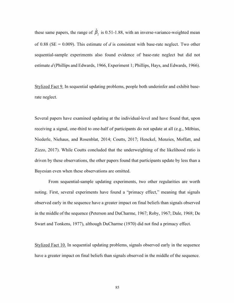
85

these same papers, the range of is 0.51-1.88, with an inverse-variance-weighted mean

of 0.88 (SE = 0.009). This estimate of d is consistent with base-rate neglect. Two other

sequential-sample experiments also found evidence of base-rate neglect but did not

estimate d (Phillips and Edwards, 1966, Experiment 1; Phillips, Hays, and Edwards, 1966).

Stylized Fact 9. In sequential updating problems, people both underinfer and exhibit base-

rate neglect.

Several papers have examined updating at the individual-level and have found that, upon

receiving a signal, one-third to one-half of participants do not update at all (e.g., Möbius,

Niederle, Niehaus, and Rosenblat, 2014; Coutts, 2017; Henckel, Menzies, Moffatt, and

Zizzo, 2017). While Coutts concluded that the underweighting of the likelihood ratio is

driven by these observations, the other papers found that participants update by less than a

Bayesian even when these observations are omitted.

From sequential-sample updating experiments, two other regularities are worth

noting. First, several experiments have found a “primacy effect,” meaning that signals

observed early in the sequence have a greater impact on final beliefs than signals observed

in the middle of the sequence (Peterson and DuCharme, 1967; Roby, 1967; Dale, 1968; De

Swart and Tonkens, 1977), although DuCharme (1970) did not find a primacy effect.

Stylized Fact 10. In sequential updating problems, signals observed early in the sequence

have a greater impact on final beliefs than signals observed in the middle of the sequence.

β2

86

The primacy effect is predicted by prior-biased updating, as discussed further in Section 8.

Second, several studies have found a “recency effect,” meaning that the most

recently observed signals have a greater impact on final beliefs than signals observed in

the middle of the sequence (e.g., Pitz and Reinhold, 1968; Shanteau, 1970, Study 2; Marks

and Clarkson, 1972; Edenborough, 1975; Grether, 1992, Experiment 3).45

Stylized Fact 11. In sequential updating problems, the most recently observed signals have

a greater impact on final beliefs than signals observed in the middle of the sequence.

The recency effect is predicted by base-rate neglect, as discussed further in Section 6. Both

primary and recency effects provide further evidence against the “pooling” hypothesis, and

hence constitute additional evidence for Stylized Fact 8.46

Section 5. Theories of Biased Inference

Most of the stylized facts outlined in the previous section had already been

identified fifty years ago in the psychology literature on bookbag-and-poker-chip

45 Unfortunately, it seems that there have been no experiments that aimed to identify both primacy and recency effects. Indeed, the typical experiment on “order effects” in this literature compares participants’ posteriors after two sequences, one whose first half is mostly a signals and whose second half is mostly b signals, and another which is the reverse. Such a design can only identify which of the two effects dominates, and indeed, much of the literature has been framed in terms of whether there is a primacy or a recency effect. 46 What is the effect of feedback and training on updating in sequential-sample experiments? Unfortunately, there is only a small amount of evidence, which I judge to be inconclusive. Phillips and Edwards (1966, Study 2) had their experimental participants report posteriors after each signal and told their experimental participants the true state after each of four 20-signal sequences. Posteriors were closer to Bayesian at the end of the fourth sequence than at the end of the first sequence but remained not extreme enough. Strub (1969) ran a sequential-sample updating experiment among a group of naïve participants and a group of trained participants, undergraduates who had received 114 hours of lecture sessions, demonstrations, problem-solving sessions, and other training in dealing with probabilities, including prior participation in bookbag-and-poker-chip experiments. Relative to the naïve participants, the trained participants had final posteriors that were much closer to Bayesian on average across updating problems, but the results are not reported in enough detail to evaluate whether the trained participants had biased beliefs in the updating problems considered separately.

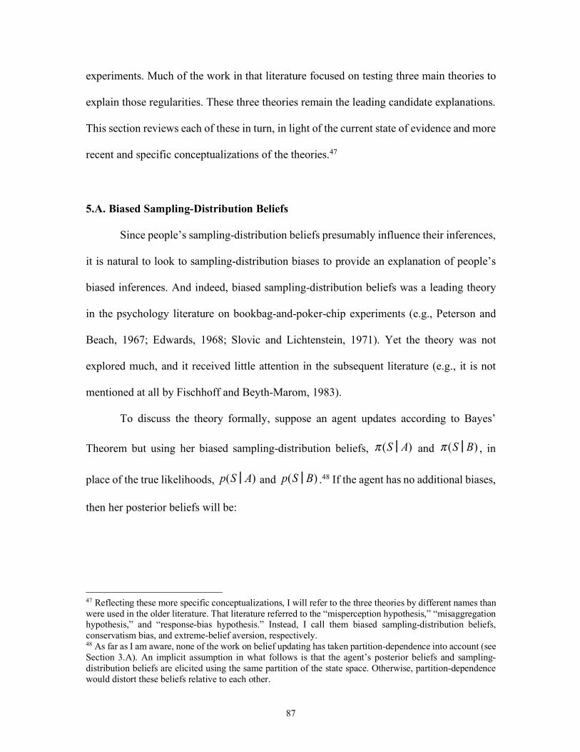
87

experiments. Much of the work in that literature focused on testing three main theories to

explain those regularities. These three theories remain the leading candidate explanations.

This section reviews each of these in turn, in light of the current state of evidence and more

recent and specific conceptualizations of the theories.47

5.A. Biased Sampling-Distribution Beliefs

Since people’s sampling-distribution beliefs presumably influence their inferences,

it is natural to look to sampling-distribution biases to provide an explanation of people’s

biased inferences. And indeed, biased sampling-distribution beliefs was a leading theory

in the psychology literature on bookbag-and-poker-chip experiments (e.g., Peterson and

Beach, 1967; Edwards, 1968; Slovic and Lichtenstein, 1971). Yet the theory was not

explored much, and it received little attention in the subsequent literature (e.g., it is not

mentioned at all by Fischhoff and Beyth-Marom, 1983).

To discuss the theory formally, suppose an agent updates according to Bayes’

Theorem but using her biased sampling-distribution beliefs, and , in

place of the true likelihoods, and .48 If the agent has no additional biases,

then her posterior beliefs will be:

47 Reflecting these more specific conceptualizations, I will refer to the three theories by different names than were used in the older literature. That literature referred to the “misperception hypothesis,” “misaggregation hypothesis,” and “response-bias hypothesis.” Instead, I call them biased sampling-distribution beliefs, conservatism bias, and extreme-belief aversion, respectively. 48 As far as I am aware, none of the work on belief updating has taken partition-dependence into account (see Section 3.A). An implicit assumption in what follows is that the agent’s posterior beliefs and sampling-distribution beliefs are elicited using the same partition of the state space. Otherwise, partition-dependence would distort these beliefs relative to each other.

π (S Ɉ A) π (S Ɉ B)

p(S Ɉ A) p(S Ɉ B)

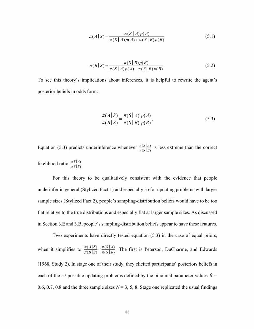
88

(5.1)

. (5.2)

To see this theory’s implications about inferences, it is helpful to rewrite the agent’s

posterior beliefs in odds form:

. (5.3)

Equation (5.3) predicts underinference whenever is less extreme than the correct

likelihood ratio .

For this theory to be qualitatively consistent with the evidence that people

underinfer in general (Stylized Fact 1) and especially so for updating problems with larger

sample sizes (Stylized Fact 2), people’s sampling-distribution beliefs would have to be too

flat relative to the true distributions and especially flat at larger sample sizes. As discussed

in Section 3.E and 3.B, people’s sampling-distribution beliefs appear to have these features.

Two experiments have directly tested equation (5.3) in the case of equal priors,

when it simplifies to . The first is Peterson, DuCharme, and Edwards

(1968, Study 2). In stage one of their study, they elicited participants’ posteriors beliefs in

each of the 57 possible updating problems defined by the binomial parameter values =

0.6, 0.7, 0.8 and the three sample sizes N = 3, 5, 8. Stage one replicated the usual findings

π (AɈS) = π (S Ɉ A)p(A)π (S Ɉ A)p(A)+π (S Ɉ B)p(B)

π (B ɈS) = π (S Ɉ B)p(B)π (S Ɉ A)p(A)+π (S Ɉ B)p(B)

π (AɈS)π (B ɈS)

= π (S Ɉ A)π (S Ɉ B)

p(A)p(B)

π (S Ɉ A)π (S Ɉ B)

p(S Ɉ A)p(S Ɉ B)

π (AɈS)π (B ɈS)

= π (S Ɉ A)π (S Ɉ B)

θ

89

of underinference on average and greater underinference with larger N and larger . In

stage two, Peterson et al. elicited nine binomial sampling distributions, with each of the

binomial parameter values = 0.6, 0.7, 0.8 and each of the three sample sizes N = 3, 5, 8.

As previously mentioned in Section 3.E, Peterson et al. found that participants’ sampling

distributions were nearly correct for N = 3 but were flatter than the correct distributions for

N = 5 and especially for N = 8. Peterson et al. tested equation (5.3) by comparing the

distributions produced in stage two to the inferences elicited in stage one.49 When they

plotted experimental participants’ median log-posterior-odds calculated from stage two,

, against participants’ log-likelihood-odds calculated from stage one,

, they found that “most points cluster extremely close to the identity line” (p.

242).50

The other paper is Wheeler and Beach (1968). Their study also had a sequence of

stages. In the first stage, participants reported their beliefs about two binomial sampling

distributions, with parameter values = 0.6 and 0.8, both with a sample size of N = 8. As

previously mentioned in Section 3.E, these sampling distributions were too flat. In the

49 Peterson et al.’s study had two further stages. Stage three was designed to de-bias participants’ sampling-distribution beliefs. Stage four repeated stage one, with no sampling distributions visible to the participants. The purpose of stage four was to test whether the de-biasing of participants’ sampling-distribution beliefs from stage three also de-biased their inferences. Peterson et al. found that underinference was reduced in stage four relative to stage one, but they do not report participants’ sampling-distribution beliefs in stage three. Thus it is not possible to assess the consistency between these beliefs and participants’ posteriors in stage four. 50 There were a few exceptions, which occurred in updating problems where the observed sample was in the far tail of the sampling distribution: 0, 1, 7, or 8 a’s out of 8, and 0 or 5 a’s out of 5. In these cases, participants inferred more strongly than would be expected given their sampling distributions. Peterson et al. suggested that these exceptions may be driven by participants assigning probabilities many times too high to these very unlikely samples, which have true probabilities smaller than 1%. While participants were allowed to estimate likelihoods smaller than 1%, Peterson et al. noted that doing so was inconvenient in their design. Peterson et al. also noted that the discrepancies could also be due to the fact that estimation errors in very small likelihoods can have a large effect on the likelihood odds.

θ

θ

ln π (AɈS)π (B ɈS)

⎛⎝⎜

⎞⎠⎟

ln π (S Ɉ A)π (S Ɉ B)

⎛⎝⎜

⎞⎠⎟

θ

90

second stage, participants bet on whether particular samples of size 8 (e.g., 6 a’s out of 8)

came from an urn where the rate of a signals was 0.6 or an urn where the rate was 0.8. The

prior probabilities of the two urns were equal. After each of 100 bets, which were

incentivized, participants were told which urn was correct. To test equation (5.3), Wheeler

and Beach compared the first 20 bets with participants’ initial sampling distributions.51

Their results were similar to Peterson et al.’s: there was a tight correspondence between

inferences and sampling-distribution beliefs.

Both of these studies support the theory that people’s inferences are consistent with

Bayes’ Theorem applied to their beliefs about sampling distributions. Both also suggest

that the flatness of these distributions may account for the general finding of

underinference. However, both had small numbers of participants: only 24 undergraduates

in Peterson, DuCharme, and Edwards and 17 in Wheeler and Beach.

There is other, less direct evidence bearing on the biased-sampling-distribution

theory of biased inferences. In particular, if the theory were true, then features of people’s

sampling-distribution beliefs (reviewed in Section 3) would be reflected in their inferences

(reviewed in Section 4). I outline three of these possible links in turn, with the caveat that

the evidence is thin regarding the latter two features of people’s sampling-distribution

beliefs.

51 Like Peterson et al., Wheeler and Beach found that in inference problems with sample realizations in the tails, participants inferred more strongly than would be expected given their sampling distributions. Wheeler and Beach’s study had further stages after the initial set of 100 bets: participants’ sampling distributions were re-elicited, then they faced another 100 bets, their sampling distributions were elicited one last time, and then they faced a final 20 bets. The purpose of this procedure was to give participants feedback and experience about the sampling distributions. Participants’ sampling distributions elicited at the beginning of the study were somewhat too peaked rather than too flat. In addition to testing equation (5.3) with data from the initial bets, Wheeler and Beach also tested it with data from the end of the study, comparing participants’ 20 bets with their final sampling distributions, and they again found a tight correspondence.

91

First, in non-small samples—e.g., a sample size of at least 10—people’s subjective

sampling distributions are based on the proportion of a signals rather than the number of a

signals (see Section 3.B). As Kahneman and Tversky (1972a) pointed out, if people’s

inferences are based on these distributions, then, for non-small sample sizes, people’s

inferences will depend on the sample proportion, as they indeed seem to (Stylized Fact 4).

Second, there is some evidence that people’s sampling-distribution beliefs

overweight the mean (see Section 3.D). If so, people put too much weight on sample

proportions matching the population rate. This feature of sampling-distribution beliefs may

explain “exact representativeness,” the (not entirely robust) evidence that overinference

occurs when the sample proportion matches the rate of one of the states (Stylized Fact 5).

Third, there is a bit of evidence that people’s sampling-distribution beliefs have flat

tails (see Section 3.C). This may be why people underinfer by more when the rates in the

two states are further apart (Stylized Fact 6). If (say) the state is A, then the most likely

samples will have sample proportions close to . The agent will overestimate the

likelihood of these samples in state B because the agent’s state-B sampling distribution has

fat tails and will therefore underinfer on average—and this overestimation and consequent

underinference will be more severe the further apart are and .

Thus, the biased-sampling-distribution theory may be consistent with nearly all of

the stylized facts regarding biased inference reviewed in Section 4, with one important

exception: the theory almost certainly cannot explain why underinference occurs on

average in samples of size one (Stylized Facts 3 and 9). In order for the theory to do so,

people would have to believe that the probability of an a signal in a single draw when the

θ A

θ A θB

92

rate is known to be is not equal to . As noted in Section 3.E, I am not aware of any

direct evidence, but such a result seems implausible.

Several of the biases in people’s sampling-distribution beliefs discussed above have

not been captured in formal models. However, two features of people’s subjective sampling

distributions—generally being too flat and being based on the proportion of a signals in

large samples—are reflected in Benjamin, Rabin, and Raymond’s (2016) model of Non-

Belief in the Law of Large Numbers (NBLLN). In addition to drawing out the implications

of NBLLN for sampling-distribution beliefs, Benjamin et al. explored implications of

NBLLN for biased inferences in economic settings, under the assumption of equations

(5.1)-(5.2).52

52 Edwards (1968, pp. 34-35) sketched a different model of biased sampling distribution beliefs:

, where , and similarly for beliefs about state B. The agent has correct

sampling-distribution beliefs if and uniform-distribution beliefs if , while if , the agent’s subjective sampling distribution is flatter than the true distribution, so the agent underinfers on average. Edwards also pointed out that in symmetric updating problems ( ), the denominators in

states A and B are equal, so . Therefore, in symmetric updating problems, the

parameter is equal to the measure of biased inference c in equation (4.6). While Edwards’s analysis stopped here, the model could be extended to capture sample-size neglect by replacing the constant with

a decreasing function of sample size, with and for N large, where is a

constant. Because , the agent’s sampling-distribution beliefs are correct when N = 1. In this model, for a large sample of binomial signals, it can be shown that the agent’s subjective sampling distribution over

sample proportions, , converges to a doubly-truncated normal distribution, , where

is the pdf of a normal distribution with mean and variance , is its cdf, and the distribution

is truncated at 0 and 1. In this formula for the “universal distribution,” the parameter enters the variance the way a sample size would, so it can be interpreted as the universal distribution’s “effective sample size.” Relative to Benjamin, Rabin, and Raymond’s model of NBLLN, this model has several disadvantages: it is less tractable for some purposes because the mean of the large-sample distribution of proportions is not equal to (it is biased toward 0.5), and it is more difficult to combine with models of biased beliefs about random sequences.

θ θ

π (Na = na Ɉ A) =p(Na = na Ɉ A)

ϕ

Σn=1N p(Na = n Ɉ A)

ϕ ϕ ∈[0,1]

ϕ = 1 ϕ = 0 0 <ϕ <1

θ A = 1−θBπ (Na = na Ɉ A)π (Na = na Ɉ B)

=p(Na = na Ɉ A)p(Na = na Ɉ B)

⎛

⎝⎜⎞

⎠⎟

ϕ

ϕϕ

ϕ(N ) ϕ(1) = 1 ϕ(N )→⌣ϕN

> 0 ⌣ϕϕ(1) = 1

πNaN

= x Ɉ A⎛⎝⎜

⎞⎠⎟

φ(x)Φ(1)−Φ(0)

φ θ Aθ A(1−θ A)⌣ϕ Φ

⌣ϕ

θ A

93

In their model, signals are drawn i.i.d. from a binomial distribution whose rate of a

signals is . The agent correctly understands that the probability of a single signal being a

is , but her subjective sampling distribution is biased for sample sizes N larger than one.

The Law of Large Numbers implies that, as , the true sampling distribution over

the proportion of a signals, , converges to a point mass at . As explained in

Section 3.B, the agent instead believes that the sampling distribution of converges

to a “universal distribution” that has mean but full support on (0,1). Thus, the agent’s

subjective sampling distribution for large samples is very flat relative to the true sampling

distribution.

When combined with equations (5.1)-(5.2), the model’s basic implications for

inference are straightforward. Let the agent’s universal distributions for binomials with

rates and be denoted and , respectively. From equation

(5.3), the agent’s posterior odds after observing a large sample containing a-signals

will be

(5.4)

Equation (5.4) formalizes two of the links between sampling-distribution beliefs

and biased inferences that have already been noted above. First, since the universal

distributions are based on sample proportions, so are the agent’s inferences in a large

θ

θ

N→∞

Na / N θ

Na / N

θ

θ A θB π∞

NaNɈ A

⎛⎝⎜

⎞⎠⎟

π∞

NaNɈ B

⎛⎝⎜

⎞⎠⎟

Na

π (AɈNa out of N )π (B ɈNa out of N )

=π∞

NaNɈ A

⎛⎝⎜

⎞⎠⎟

π∞

NaNɈ B

⎛⎝⎜

⎞⎠⎟

p(A)p(B)

94

sample. Second, in large samples, because the agent’s subjective sampling distribution is

too flat, the agent underinfers. Furthermore, while the Bayesian will learn the true state

with certainty in an infinite sample, the agent will remain uncertain even after observing

an infinite sample. For example, if the true state is A, then (due to the Law of Large

Numbers) the sample proportion will converge to the state-A rate with probability one.

The agent’s likelihood ratio in equation (5.4) will therefore converge to ,

which is the ratio of the pdfs of the universal distributions, evaluated at . Since this

likelihood ratio is a finite number, the agent’s inference is limited.

Because the likelihood ratio is finite, it is clear from equation (5.4) that the agent’s

priors will continue to matter no matter how large a sample the agent observes. For this

reason, Benjamin, Rabin, and Raymond argue that NBLLN can serve as an “enabling bias”

for misbeliefs people have about themselves. In particular, if people have overoptimistic

priors about their own abilities or preferences (for reasons unrelated to NBLLN), NBLLN

may explain why they remain overoptimistic despite a lifetime of experience.

Benjamin, Rabin, and Raymond also explored the implications of NBLLN for

people’s demand for information. What is crucial for demand for information is what the

agent expects to infer. While a Bayesian’s expectations about his own inferences are

correct, an agent with NBLLN has incorrect expectations because she has mistaken beliefs

about the distribution of samples she will observe. Surprisingly, these mistaken beliefs can

cause the agent to have greater willingness to pay for an intermediate-sized sample than a

Bayesian would have. In particular, because the agent’s subjective sampling distribution is

θ A

π∞

NaN

= θ A Ɉ A⎛⎝⎜

⎞⎠⎟

π∞

NaN

= θ A Ɉ B⎛⎝⎜

⎞⎠⎟

θ A

95

too flat, she thinks an extreme proportion of a signals that would be very informative about

the state is more likely than it is. The agent may be willing to pay for the sample in the

hope of such an extreme sample realization, even though a Bayesian would recognize that

such an outcome is too unlikely to be worth paying for.

For a large sample, however, the agent anticipates drawing a weaker inference than

a Bayesian would draw for any possible realization of the sample proportion (because a

Bayesian will learn the truth in a large enough sample, while the agent’s inference will be

limited). Therefore, an agent with NBLLN always has lower willingness to pay for a large

sample than a Bayesian would have. Benjamin, Rabin, and Raymond argue that this lack

of demand for large samples is a central implication of NBLLN, which may contribute to

explaining why statistical data is rarely provided by the market, as well as why people often

rely on anecdotes rather than seeking larger samples.

For drawing out the implications of biased inferences when samples are observed

sequentially, a crucial issue is how people group signals, as discussed in Section 4.C. For

an agent with NBLLN, it makes all the difference whether 100 signals are grouped as a

single sample, in which case she dramatically underinfers, or as 100 samples of size one,

in which case she updates correctly after each signal and ends up with the same posteriors

as a Bayesian!

As per Stylized Fact 8, there is evidence against the hypothesis that people “pool”

all signals they have observed into a single large sample. It may therefore be reasonable to

hypothesize that people are “acceptive” of the way signals are presented to them,

processing signals as a sample when the signals are presented together. This evidence,

however, relates only to how signals are grouped retrospectively, after they are observed.

96

The implications of NBLLN in many dynamic environments also depends on how the agent

expects to group signals she hasn’t yet observed. There is no necessary reason why people

would prospectively group signals the same way they retrospectively group signals.

Differences between retrospective and prospective grouping can generate dynamically

inconsistent behavior. An important lesson that emerges from formally modeling NBLLN

is the need for evidence on how people group signals both retrospectively and

prospectively.

5.B. Conservatism Bias

The theory of biased inference that received by far the most attention in the

literature on bookbag-and-poker-chip experiments is conservatism bias: when updating to

posterior beliefs, people underweight their likelihood beliefs. Phillips and Edwards (1966)

introduced conservatism bias and modeled it as

. (5.5)

Formally, this equation is the special case of equation (4.6) in which biased use of prior

information is abstracted away (d = 1). Conceptually, however, there is a key difference:

whereas equation (4.6) is intended as a reduced-form description used to summarize

evidence from updating problems, conservatism bias is a structural model of the actual

process of forming beliefs. Psychologically, conservatism bias is hypothesized to result

from the difficulty of aggregating different sources of information (e.g., Slovic and

Lichtenstein, 1971).

π (AɈS)π (B ɈS)

= p(S Ɉ A)p(S Ɉ B)

⎡

⎣⎢

⎤

⎦⎥

cp(A)p(B)

97

In a comparison with other theories of biased inference, Edwards (1968) cites three

pieces of evidence in favor of conservatism bias. First, in several sequential-sample

updating experiments conducted with symmetric binomial signals, estimates of the

conservatism parameter c were found to be roughly independent of the numbers of a and b

signals that occurred in a sample (Phillips and Edwards, 1966, Experiments 1 and 3;

Peterson, Schneider, and Miller, 1965, as reported by Edwards, 1968; also in a

multinomial-signal experiment: Shanteau, 1972).53 This stability of estimates of c

supported its interpretation as a structural parameter, and it is a challenging fact for

alternative theories to explain.54 It should be noted, however, that estimates of c were

known to be smaller when the diagnosticity parameter was larger (Phillips and Edwards,

1966) and, in sequential-sample experiments, when the sample size N was larger (Peterson,

Schneider, and Miller, 1965), as per Stylized Facts 6 and 2. While there was no clear

explanation for the dependence on , greater conservatism for larger sample sizes had a

ready interpretation: aggregating more information is more difficult.

Second, in settings where participants themselves provide the likelihood estimates,

participants nonetheless update too little relative to Bayes’ Theorem (e.g., Hammond,

Kelly, Schneider, and Vancini, 1967; Grinnell, Keeley, and Doherty, 1971). For example,

in some experiments, participants were asked to estimate the likelihood of different signals

(e.g., reconnaissance reports) in different states of the world (e.g., impending war), and

53 At first blush, this observation seems inconsistent with “exact representativeness”—stronger inferences when the observed sample proportion equals the rate in one of the states—as per Stylized Fact 5. However, the estimates of the conservatism parameter c presented in these papers were averaged across sample sizes, so it is not possible to assess whether or not there was evidence of exact representativeness. 54 The model of sampling-distribution beliefs sketched in footnote 52 does imply that, in symmetric binomial updating problems, the measure of biased inference c is independent of the numbers of a and b signals in the sample. For Edwards (1968), explaining that observation was an important desideratum for evaluating a theory of underinference.

θ

θ

98

then they observed certain signals and were asked to update their beliefs (e.g., Edwards,

Phillips, Hays, Goodman, 1968). In such an experiment, participants’ biased posteriors

cannot be attributed to biased sampling-distribution beliefs because the perceived

likelihoods are elicited directly. This evidence, however, is not sufficient to conclude that

participants update too little relative to Bayes’ Theorem. One concern is that, while

participants provide point estimates of the likelihoods, participants may in fact be uncertain

about the likelihoods or report their point estimates with error. In either case, Bayes’

Theorem applied to participants’ point estimates is the wrong benchmark for comparing

with participants’ posteriors. Another concern is that Bayes’ Theorem was calculated

assuming that the signals are independent conditional on the states, but participants’ beliefs

about the likelihoods were typically not elicited in sufficient detail to test that assumption.

Third, people underinfer for sample sizes of one (Stylized Facts 3 and 9). This

observation can be explained by conservatism bias, while as discussed above, it is a

challenging observation to explain by biased sampling-distribution beliefs. Extreme-belief

aversion, discussed next, is a competing explanation for this observation.

5.C. Extreme-Belief Aversion

Extreme-belief aversion is the term used by Benjamin, Rabin, and Raymond (2016,

Appendix C) to refer to an aversion to holding or expressing beliefs close to certainty.55 As

a simple example, suppose there are two possible states, A and B, and the true probability

of A is p. An agent with extreme-belief aversion would report that the probability of A is

, where for p sufficiently close to 0 and for p sufficiently

55 The more general term “extremeness aversion” is sometimes used to refer to a desire to avoid both extreme judgments and extreme choices (e.g., Lewis, Gaertig, and Simmons, 2018).

π = f ( p) f ( p) > p f ( p) < p

99

close to 1. Note that extreme-belief aversion is not specifically a theory of biased inference

but rather a theory about bias in any beliefs.56

DuCharme (1970) argued that extreme-belief aversion is a major confound in

belief-updating experiments that explains much of the evidence that had been interpreted

as underinference. In support of this view, DuCharme reported two experiments. Both were

sequential-sample bookbag-and-poker-chip experiments with two states and normally

distributed signals. Using the results of each experiment, DuCharme produced a plot like

Figure 2, graphing participants’ log posterior odds ( ) against the Bayesian log

posterior odds ( ). Both experiments resulted in similar plots: for Bayesian odds

between -1 and +1, participants’ odds virtually coincided with the Bayesian odds, but for

Bayesian odds more extreme than -1 or +1, participants’ odds were less extreme than the

Bayesian odds. The plot was similar whether or not the data was restricted to the posteriors

reported by participants after just a single signal had been observed. In an earlier paper that

also reported two experiments with normally distributed signals, DuCharme and Peterson

(1968) had found similar results. The results of these experiments are difficult to reconcile

with conservatism bias but consistent with extreme-belief aversion.

56 Extreme-belief aversion resembles probability weighting but is conceptually distinct. Probability weighting is a bias in how beliefs are used in decision making (rather than a bias in how they are formed or reported); it is discussed in Chapter XXX (by O’Donoghue and Sprenger) of this Handbook. Extreme-belief aversion is also distinct from an aversion to reporting a response at the extremes of the response scale, a bias that is sometimes called floor and ceiling effects. Such floor and ceiling effects have been documented in bookbag-and-poker-chip experiments. For example, experimental participants report less extreme beliefs when reporting their beliefs as probabilities, which are bounded between zero and one, than when reporting their beliefs as odds or log-odds, which have a response scale that is unbounded on at least one end (Phillips and Edwards, 1966, Experiment III). However, floor and ceiling effects seem unlikely to account for DuCharme and Peterson’s (1968) evidence mentioned below because they elicited respondents’ posterior odds, so the response scale did not have a floor or ceiling.

ln π1−π

⎛⎝⎜

⎞⎠⎟

ln p1− p

⎛⎝⎜

⎞⎠⎟

100

Extreme-belief aversion is a distortion toward less extreme posteriors that does not

depend on whether the correct posteriors are extreme due to an extreme likelihood or an

extreme prior. Thus, extreme-belief aversion is a confound not only for findings that have

been interpreted as underinference (Stylized Fact 1) but also those that have been

interpreted as base-rate neglect (Stylized Fact 7). Moreover, the extreme-belief aversion

explanation of these findings applies equally to sequential-sample and simultaneous-

sample experiments (Stylized Fact 9) and to samples of any size. In particular, extreme-

belief aversion provides an explanation for the apparent evidence of underinference after

just a single signal (Stylized Fact 3), a fact that biased sampling-distribution beliefs cannot

explain.

Based on the particular shape of extreme-belief aversion observed in his plots of

the results mentioned above, DuCharme (1970) argued that the bias can also explain the

evidence that has been interpreted as underinference being more severe on average when

sample sizes are larger (Stylized Fact 2) and when the population rates and are

further apart (Stylized Fact 6).57 These stylized facts are based on measuring the amount

of underinference by c, which is equal to in updating problems with

equal priors (see Section 4.A and the discussion of Figure 2 in Section 4.B). DuCharme’s

plots imply that when the Bayesian log posterior odds are within the interval [-1,+1],

but when the Bayesian odds are more extreme. Both larger sample sizes and

57 These stylized facts are not implied by the general definition of extreme-belief aversion given above. For example, an extreme-belief averse agent could have posterior beliefs such that for some

constant . In that case, the measure of underinference c would be equal to regardless of how

extreme the Bayesian posterior odds are. If extreme-belief aversion took this form, then DuCharme’s

plot would have been a line through zero with slope .

θ A θB

ln π1−π

⎛⎝⎜

⎞⎠⎟/ ln p

1− p⎛⎝⎜

⎞⎠⎟

c ≈1

c <1

ln π1−π

⎛⎝⎜

⎞⎠⎟= χ ln p

1− p⎛⎝⎜

⎞⎠⎟

χ ∈(0,1) χ

ln p1− p

⎛⎝⎜

⎞⎠⎟

χ

101

population rates that are further apart make the expected Bayesian odds more extreme,

leading in expectation to more severe underinference as measured by c.

The theory of extreme-belief aversion has not been developed in much detail. It is

worth exploring whether extreme-belief aversion is actually the same phenomenon as

compression of probabilities toward a uniform distribution, discussed in Section 3.A in the

context of partition dependence. Such compression would indeed lead people to avoid

reporting beliefs close to certainty. Whether or not the two biases are the same, they raise

similar conceptual challenges.

Extreme-belief aversion probably contributes to biased updating, and it is a

certainly a confound that should be taken into account when interpreting the evidence from

updating experiments. However, Benjamin, Rabin, and Raymond (2016, Appendix C)

argued that the stylized facts discussed in Section 4 cannot be entirely attributed to

extreme-belief aversion. If extreme-belief aversion were the only bias at play, then

experimental participants’ reported posteriors ( ) would be a fixed transformation of the

correct posteriors ( ). That implies that in any two problems where the correct

posteriors are the same, experimental participants’ reported posteriors would also be the

same. There are several clean test cases that contradict this prediction. For example,

consider four of the updating problems in Griffin and Tversky’s (1992, Study 1) belief-

updating experiment (described in Section 4.B): 3 out of 3 a signals, 4 out of 5 a signals, 6

out of 9 a signals, and 10 out of 17 a signals. Because the difference between the number

of a and b signals is always 3, the correct posterior is the same in all four problems.

Experimental participants’ median posteriors, however, were less extreme in the problems

with larger sample sizes. Other, similar examples from Griffin and Tversky (1992)’s Study

π

π = f ( p)

102

1 and Kraemer and Weber (2004) also provide evidence of Stylized Fact 2 that is

unconfounded by extreme-belief aversion.

Analogously, there are examples from Griffin and Tversky’s (1992) Study 2 where

the correct posteriors are the same across updating problems with different prior

probabilities. Consistent with base-rate neglect (Stylized Fact 7), participants’ posteriors

were less extreme in the problems with more extreme priors. Similarly, Griffin and

Tversky’s (1992) Study 3 and Kahneman and Tversky (1972a) provide evidence,

unconfounded by extreme-belief aversion, that participants underinfer when the rates

and are further apart (Stylized Fact 6) and draw inferences based on sample proportions

(Stylized Fact 4).

5.D. Summary

There is evidence for all three of the theories reviewed in this section: biased

sampling-distribution beliefs, conservatism bias, and extreme-belief aversion. Biases in

sampling-distribution beliefs are a natural starting point and may explain many of the

stylized facts about biased inference from Section 4. To date, however, formal models of

people’s sampling-distribution beliefs capture only some of the relevant biases. In my

judgment, this theory is particularly ripe for theoretical development and application in

field settings. Evidence on how people group signals is needed in order to understand how

the biases play out in dynamic settings.

Biased sampling-distribution beliefs seem unlikely to explain why people

underinfer from single signals, whereas extreme-belief aversion and conservatism bias

θ A

θB

103

could explain that evidence. In my view, experiments designed to disentangle the theories

from each other and assess their relative magnitudes should be a priority.

104

Section 6. Base-Rate Neglect

The evidence reviewed in Section 4 indicates that in updating problems, with or

without incentives for accuracy, people on average under-use prior information (Stylized

Facts 7 and 9). This phenomenon was apparent from the psychology literature on bookbag-

and-poker-chips—indeed, it was documented by Phillips and Edwards (1966, Experiment

1) in one of the first such experiments—but it was largely ignored in that literature.

Kahneman and Tversky (1973) made this bias a focus of attention in the literature on errors

in probabilistic reasoning and labeled it base-rate neglect.

Among various other surveys and experiments, Kahneman and Tversky (1973)

presented an elegant demonstration of base-rate neglect and its properties. They asked

experimental participants to assign a probability to the event that Jack is an engineer rather

than a lawyer based on the following description:

Jack is a 45 year old man. He is married and has four children. He is

generally conservative, careful, and ambitious. He shows no interest in

political and social issues and spends most of his free time on his many

hobbies which include home carpentry, sailing, and mathematical puzzles.

There were two groups of participants. Both were provided the same description, but one

group was told that it was randomly drawn from a set of 100 descriptions consisting of 30

engineers and 70 lawyers, while the other was told that the set included 70 engineers and

30 lawyers. Although we do not know participants’ assessment of the likelihood ratio based

on the description, , Bayes’ Theorem (equation (4.3)) implies that the first group of π (S Ɉ A)π (S Ɉ B)

105

subjects should have posterior odds , and the second group should have

posterior odds . Bayes’ Theorem therefore allows us to make an unambiguous

prediction about the ratio of the posterior odds across the two groups: it should be

» 5.4. Contrary to this, the first group’s mean probability that Jack is an engineer (averaged

across this description and four similar others) was 55%, and the second group’s was 50%,

yielding a ratio of only » 1.2. Thus, manipulation of the base rates had less of an

effect on the posterior probabilities than would be prescribed by Bayes’ Theorem. Such

base-rate neglect in response to the description of Jack has been replicated many times, but

whereas Kahneman and Tversky found complete neglect of base rates, in some other

experiments, participants’ posteriors reflected the base rates to some extent but less than

they should according to Bayes’ Rule (Koehler’s (1996) Table 1).

To provide some insight when base-rate neglect occurs, Kahneman and Tversky

then conducted two more versions of the same experiment. In one version, participants

were given “no information whatsoever about a person chosen at random from the sample.”

In that case, participants reported probabilities that were equal to the base rates. Thus, in

the absence of updating, participants understood the base rates correctly, and no base-rate

neglect occurred.

In the other version of the experiment, participants were given the following

description, which was intended to be completely uninformative regarding whether the

person is a lawyer or engineer:

π (S Ɉ A)π (S Ɉ B)

0.700.30

π (S Ɉ A)π (S Ɉ B)

0.300.70

0.70 / 0.300.30 / 0.70

0.55 / 0.450.50 / 0.50

106

Dick is a 30 year old man. He is married with no children. A man of high

ability and high motivation, he promises to be quite successful in his field.

He is well liked by his colleagues.

In this case, in both the 70%-30% and the 30%-70% groups, the median probability

assigned to Dick being an engineer was 50%—implying complete base-rate neglect in this

case. Participants relied on the description to make their judgment, even though the

description was uninformative. Some subsequent experiments have also found base-rate

neglect in response to uninformative descriptions (Wells and Harvey, 1978; Ginosar and

Trope, 1987), but others instead found that participants’ posteriors were equal to their

priors (Swieringa et al., 1976; Ginosar and Trope, 1980; Fischhoff and Bar-Hillel, 1984;

Hamilton, 1984). Manipulating the instructions, participant pool, and implementation of

the experiment, Zukier and Pepitone (1984) and Gigerenzer, Hell, and Blank (1988) found

that base-rate neglect sometimes occurs in response to uninformative descriptions and

sometimes does not. Overall, the evidence for base-rate neglect in response to an

uninformative description is much less robust than that for an informative description, but

when there is an effect, it goes in the direction of base-rate neglect.

Taken together, the results of the no-description and the uninformative-description

versions of the experiment have an important implication: base-rate neglect is triggered by

updating the prior with information from a new signal. For a base-rate neglecter, there is a

distinction between receiving no signal, in which case no updating occurs, and receiving

an uninformative signal, which may cause updating and hence base-rate neglect to occur.

For a Bayesian agent, in contrast, there would be no difference across these two cases.

107

To explain their results, Kahneman and Tversky (1973) argued that people judge

probabilities based on the “representativeness” of the personality sketch to a lawyer or

engineer, whereas the base rates are not relevant to judgments of representativeness (see

Section 7.A for further discussion). Nisbett, Borgida, Crandall, and Reed (1976) suggested

another psychological mechanism: the likelihood information is weighted more heavily

because it is “vivid, salient, and concrete,” whereas the base rates are “remote, pallid, and

abstract.” Bar-Hillel (1980) argued that base-rate neglect is more general than either of

these explanations would predict. She documented base-rate neglect in a sequence of

updating problems that specified both the base rates and the likelihoods as (abstract)

statistics. For example, one of the most famous problems is the Cab Problem (originally

due to Kahneman and Tversky, 1972b):

Two cab companies operate in a given city, the Blue and the Green

(according to the color of cab they run). Eighty-five percent of the cabs in

the city are Blue, and the remaining 15% are Green.

A cab was involved in a hit-and-run accident at night.

A witness later identified the cab as a Green cab.

The court tested the witness’ ability to distinguish between Blue and Green

cabs under nighttime visibility conditions. It found that the witness was able

to identify each color correctly about 80% of the time, but confused it with

the other color about 20% of the time.

What do you think are the chances that the errant cab was indeed Green, as

the witness claimed?

108

In this problem, the correct answer is » 41%. Bar-Hillel (1980) found

that only about 10% of her high school graduate respondents gave a response to this

question close to the correct answer. The modal answer, which was given by 36% of

respondents, was 80%. This answer reflects complete base-rate neglect. The same basic

result has been replicated many times, including with much more extreme base rates (e.g.,

99% Blue and 1% Green; Murray, Idling, Farris, and Revlin, 1987).

Bar-Hillel argued that the key variable underlying base-rate neglect is relevance:

when the base rate is the only relevant information available, people use it; when other

information is also relevant, people prioritize the information in order of relevance. Thus,

people use the base rates more when they seem more relevant to the particular instance in

the updating problem. Base-rate neglect in the Cab Problem could be explained by the

observation that many participants believed the color distribution of cabs was irrelevant,

as documented by informal interviews with respondents and experimental evidence from

Lyon and Slovic (1976). Relevance, in turn, is influenced by specificity: when people have

information about some population (e.g., 15% of cabs are Green) but also have information

about a subset of that population (e.g., a witness identified that particular cab as Green),

the latter seems more relevant for making a judgment about a member of the subset (e.g.,

the chances that the errant cab was Green). Specificity can also be achieved via a causal

relationship. For example, in a variant of the Cab Problem, Tversky and Kahneman (1980)

described the base rates by telling respondents “85% of the cab accidents in the city involve

[blue] cabs,” implying that blue cabs cause more accidents than green cabs. In this causal

framing, they found far lower rates of base-rate neglect. In a sequence of updating

(0.8)(0.15)(0.8)(0.15)+ (0.2)(0.85)

109

problems, Bar-Hillel manipulated the relevance of the base rates in different ways and

showed that the degree of base-rate neglect varied accordingly. For example, base-rate

neglect was largely eliminated in a variant of the Cab Problem where the specificity of the

likelihood information was reduced to be comparable to that of the base rate (the witness

did not see the cab but remembers hearing an intercom, which are installed in 80% of the

Green cabs and 20% of the Blue cabs).

Much subsequent research on base-rate neglect has used updating problems like the

Cab Problem, which specify both the prior probabilities and the likelihoods and are

contextualized in hypothetical, realistic scenarios. Two examples from the economics

literature are Dohmen et al. (2009), who documented widespread base-rate neglect in a

representative sample of 988 Germans, and Ganguly, Kagel and Moser (2000), who found

base-rate neglect in market experiments with financial incentives. While Bar-Hillel’s

(1980) and some other results show a high frequency of complete base-rate neglect, most

of the evidence is less extreme and instead indicates that people’s inferences usually do

incorporate base rates to some extent, albeit less fully than prescribed by Bayes’ Rule

(Koehler, 1996). The evidence from bookbag-and-poker-chip experiments reviewed in

Section 4 similarly points to underweighting of priors, rather than complete neglect (at least

on average).

Troutman and Shanteau (1977) conducted two sequential-sample bookbag-and-

poker-chip experiments whose results further suggest that it is the act of updating that

triggers base-rate neglect. Beads were drawn with replacement from one of two boxes with

equal prior probabilities. In one of the experiments, Box A contained 70/30/50

red/white/blue beads, and box B contained 30/70/50. To give a flavor of the results, after

110

an initial sample of two white beads, experimental participants’ mean probability assigned

to box A was 69.9%. The experimenter then drew a “null sample,” consisting of no beads

at all, and asked participants to update their beliefs. Participants’ mean probability declined

to 66.9% (SE of the change = 1.0%). To show that participants understood the lack of

information contained in the null sample, Troutman and Shanteau presented another

sequence in which the null sample occurred first. In that case, participants’ mean

probability was 50%.58

Much of the literature has focused on factors that increase or reduce the extent of

base-rate neglect (for reviews, see Koehler, 1996, and Barbey and Sloman, 2007). For

example, based on a literature review and two experiments, Goodie and Fantino (1999)

concluded that base-rate neglect can be reduced but nonetheless persists even after

extensive training with explicit feedback. Many papers have focused on the effect of

framing the updating problem in terms of frequencies versus probabilities. After reviewing

this literature, Barbey and Sloman (2007) conclude that frequency formats weaken base-

rate neglect but do not eliminate it.

58 Troutman and Shanteau also found in both experiments that when participants observed an “irrelevant sample” of all blue beads or a “mixed” sample of one red and one white bead—both are which are uninformative regarding A versus B—participants’ posterior probability of Box A was similarly moderated toward 50%, and these effects were larger than that of the null sample. Across several sequential-sample experiments modeled on Troutman and Shanteau’s, Labella and Koehler (2004) did not replicate this result, finding instead that participants’ posteriors were unaffected by an irrelevant sample and became more extreme after a mixed sample. (Labella and Koehler did not study the effect of a “null sample.”) However, in a simultaneous-sample version of their experiment, Labella and Koehler did find that participants’ posteriors were weaker when an additional, mixed set of signals was included in the sample. The “null sample” result is a cleaner test of whether base-rate neglect is triggered by updating because observing an irrelevant or mixed sample could affect beliefs for two additional reasons discussed in this chapter. First, it may moderate beliefs if inferences are drawn based on the sample proportion (Stylized Fact 4), including in sequential samples if inferences are based on the pooled sample. Second, it could make beliefs more extreme due to prior-biased updating (Section 8) (which is indeed how Labella and Koehler interpreted their finding of more extreme beliefs after a mixed sample).

111

Researchers have discussed the pervasiveness of base-rate neglect in a variety of

field settings, including psychologists’ interpretations of diagnostic tests (Meehl and

Rosen, 1955), courts’ judgments in trials (Tribe, 1971), and doctors’ diagnoses of patients

(Eddy, 1982). In two experiments, Eide (2011) found that law students exhibit a similar

degree of base-rate neglect in the Cab Problem as the usual undergraduate samples. In

experiments with realistic hypothetical scenarios, school psychologists were found to be

more confident but less accurate in assessing learning disability when base-rate information

was supplemented with individuating information (Kennedy, Willis, and Faust, 1997).

Benjamin, Bodoh-Creed, and Rabin (2018) analyzed the implications of a formal

model of base-rate neglect:

. (6.1)

with 0 < d < 1. Equation (6.1) is the special case of equation (4.6) in which biased

inferences are abstracted away (c = 1). However, unlike equation (4.6), equation (6.1) is

treated as a structural model of the belief-updating process. In this model, neglect of base

rates (i.e., population frequencies), as in the evidence discussed above, is treated as a

special case of underweighting priors in general. As per the evidence from Kahneman and

Tversky (1973) discussed above, it is assumed that the agent updates whenever a signal is

observed, even if the signal is uninformative.

A number of implications follow directly from equation (6.1). First, whereas a

Bayesian treats all signals symmetrically, a base-rate neglecter is affected more by recent

π (AɈS)π (B ɈS)

= p(S Ɉ A)p(S Ɉ B)

p(A)p(B)

⎡

⎣⎢

⎤

⎦⎥

d

112

than less recent signals. To see this, note that the base-rate neglecter’s posterior odds after

one signal are

;

and after two signals,

.

(6.2)

Because the older signal becomes part of the prior when the new signal arrives, the older

signal is down-weighted twice, whereas the new signal is down-weighted only once. Thus,

base-rate neglect provides an explanation of the “recency effects” observed in the bookbag-

and-poker-chip experiments (Stylized Fact 11). As discussed below, in economic settings,

these recency effects can generate adaptive expectations and extrapolative beliefs.

Second, the base-rate neglecter’s long-run beliefs fluctuate in accordance with an

ergodic (stationary long-run) distribution. Iterating the derivation of equation (6.2) and

taking the logarithm, the agent’s log posterior odds after observing t signals are ,

where denotes the log likelihood of the signal for and

denotes the log prior odds. Since this sum is an AR(1) process, it converges in the limit

to an ergodic distribution, as long as the ’s are bounded. Thus, while a Bayesian

π (AɈ s1)π (B Ɉ s1)

=p(s1 Ɉ A)p(s1 Ɉ B)

p(A)p(B)

⎡

⎣⎢

⎤

⎦⎥

d

π (AɈ s1,s2 )π (B Ɉ s1,s2 )

=p(s2 Ɉ A)p(s2 Ɉ B)

p(s1 Ɉ A)p(s1 Ɉ B)

⎡

⎣⎢

⎤

⎦⎥

dp(A)p(B)

⎡

⎣⎢

⎤

⎦⎥

d2

τ=0

t

∑dt−τ lτ

lτ ≡p(sτ Ɉ A)p(sτ Ɉ B)

τ th τ > 0 l0 ≡π (A)π (B)

t→∞ lτ

113

will eventually identify the true state with certainty, a base-rate neglecter will never

become fully confident, and her beliefs will forever fluctuate even if the environment is

fundamentally stationary.

This in turn implies that in settings where the agent observes many signals, base-

rate neglect will cause her to ultimately become underconfident about the state. Such

underconfidence contrasts with the impression one might get from examples like the Cab

Problem, where base-rate neglect causes people to be overly swayed by a signal indicative

of an event that is unlikely given the base rates. While base-rate neglect can cause people

to “jump to conclusions” after a single signal that goes in the opposite direction of the base

rates—as in almost all of the updating problems used to study base-rate neglect—in the

long run it is a force for persistent uncertainty (see Section 10.A for related discussion).

Third and finally, equation (6.1) has a counterintuitive implication that Benjamin,

Bodoh-Creed, and Rabin call the “moderation effect”: when the agent’s prior in favor of a

state is sufficiently strong, a supportive signal can dampen the agent’s belief about the

state! The moderation effect occurs because the new signal has less of an impact on the

agent’s posterior than down-weighting the prior. Although surprising, there is evidence of

the moderation effect in existing data. For example, consider the updating problems in

Griffin and Tversky’s (1992) Study 2, where the rate of a signals was 0.6 in state A and 0.4

in state B, participants were informed about a sample of size 10, and the prior probability

of state A was 90%. When the sample contained 5 a’s, participants reported a median

posterior of 60%; when 6 a’s, 70%; and when 7 a’s, 85%. In all of these cases, the

participants’ posterior belief was lower than the prior of 90%, consistent with a moderation

effect. (Their posterior belief exceeded 90% only when the sample had at least 8 a’s.)

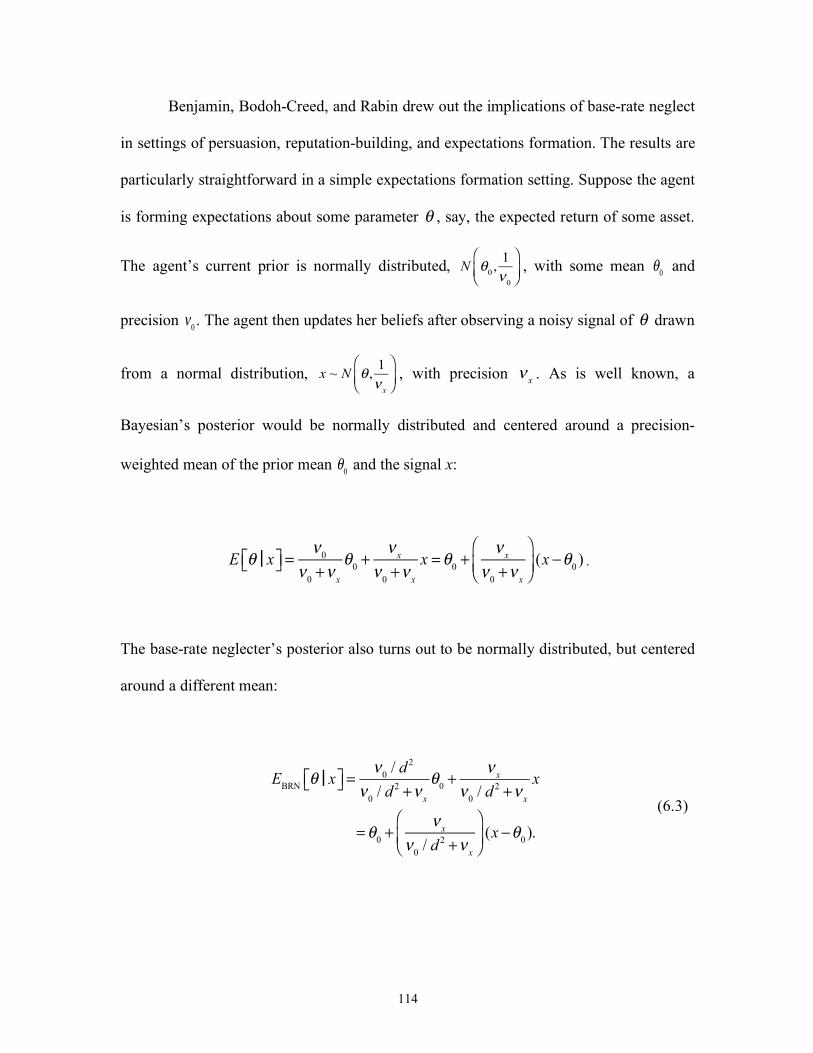
114

Benjamin, Bodoh-Creed, and Rabin drew out the implications of base-rate neglect

in settings of persuasion, reputation-building, and expectations formation. The results are

particularly straightforward in a simple expectations formation setting. Suppose the agent

is forming expectations about some parameter , say, the expected return of some asset.

The agent’s current prior is normally distributed, , with some mean and

precision . The agent then updates her beliefs after observing a noisy signal of drawn

from a normal distribution, , with precision . As is well known, a

Bayesian’s posterior would be normally distributed and centered around a precision-

weighted mean of the prior mean and the signal x:

.

The base-rate neglecter’s posterior also turns out to be normally distributed, but centered

around a different mean:

(6.3)

θ

N θ0 ,1ν0

⎛

⎝⎜⎞

⎠⎟θ0

ν0 θ

x ~ N θ , 1ν x

⎛

⎝⎜⎞

⎠⎟ν x

θ0

E θ Ɉ x⎡⎣ ⎤⎦ =ν0

ν0 +ν xθ0 +

ν xν0 +ν x

x = θ0 +ν x

ν0 +ν x

⎛

⎝⎜⎞

⎠⎟(x −θ0 )

EBRN θ Ɉ x⎡⎣ ⎤⎦ =ν0 / d

2

ν0 / d2 +ν x

θ0 +ν x

ν0 / d2 +ν x

x

= θ0 +ν x

ν0 / d2 +ν x

⎛

⎝⎜⎞

⎠⎟(x −θ0 ).

115

Because base-rate neglect causes the agent to treat the prior as less informative than it is,

the base-rate neglecter updates as if the precision of the prior distribution is shrunken by a

factor of . Consequently, as shown in equation (6.3), the agent’s expectations are overly

influenced by the recently observed signal. Such expectations can generate extrapolative

beliefs, in which the agent over-extrapolates from recent returns when predicting future

returns. As discussed in Chapter XXX (by Barberis) of this Handbook, extrapolative beliefs

are an important ingredient in explaining a variety of puzzles in finance.

When studying the implications of base-rate neglect in field settings, a crucial issue

is how people group signals (as previously discussed in Sections 4.C and 5.A). Benjamin,

Bodoh-Creed, and Rabin make the plausible assumption that beliefs are updated after each

new signal is observed, but there are other possibilities. For example, all previously

observed signals could be pooled together into a single sample. If the agent then updates

using her original priors and the pooled sample, then earlier signals would not be down-

weighted more than recent signals. While Stylized Fact 8 summarizes evidence against

such pooling, the evidence is relatively thin. In settings where the agent’s future beliefs are

relevant, it also matters whether or not the agent believes she will exhibit base-rate neglect

and how she anticipates grouping signals she may receive in the future. There is no

evidence on these issues.

d 2

116

Section 7. The Representativeness Heuristic

In his Nobel lecture, Daniel Kahneman (2002) recollected how his collaboration

with Amos Tversky began when he invited Tversky to give a guest lecture in his graduate

psychology course at Hebrew University in 1968-1969. Tversky, whom as a Ph.D. student

had been mentored by Ward Edwards, lectured about conservatism bias. Kahneman was

deeply skeptical for a number of reasons, including the everyday experience that—contrary

to conservatism bias—people commonly jump to conclusions on the basis of little data.

Kahenman’s reaction shook Tversky’s faith in thinking about people as merely a biased

version of Bayesian, and they met for lunch to discuss their experiences and hunches about

how people really judge probabilities.

Their collaboration blossomed into the enormously influential “heuristics and

biases” research program (see, e.g., Gilovich, Griffin, and Kahneman, 2002). To explain

this research program, Tversky and Kahneman (1974) drew an analogy with visual

perception. People perceive objects as physically closer when they can be seen more

sharply. This perceptual heuristic has some validity but leads to systematic errors when

visibility is unusually good or poor. Similarly, Tversky and Kahneman argued, a small

number of simple heuristics are useful for a wide range of complex probabilistic judgments

but also generate systematic biases.

7.A. Representativeness

The first heuristic Kahneman and Tversky (1972a) proposed—and the central one

for probabilistic reasoning—is the representativeness heuristic. They defined it as

“evaluat[ing] the probability of an uncertain event, or a sample, by the degree to which it

117

is: (i) similar in essential properties to its parent population; and (ii) reflects the salient

features of the process by which it is generated” (p. 431).59 Across several papers

(Kahneman and Tversky, 1972a, 1973; Tversky and Kahneman, 1983), Kahneman and

Tversky argued that the representativeness heuristic is the psychological process that

generates the LSN (Section 2.A), sample-size neglect (Section 3.A), and base-rate neglect

(Section 6), as well as several other biases such as the conjunction fallacy (described

below).60 For each of these biases, Kahneman and Tversky reported evidence from many

different surveys and experiments.

Kahneman and Tversky (1972a) focused on people’s beliefs about random samples.

They argued that in order for a sample to be representative of the population from which it

is drawn, it must satisfy both parts of the definition of representativeness: (i) the sample

proportions must match the population rate, and (ii) systematic patterns must be absent.

They called part (i) the LSN, and some of the evidence is described in Section 2.A. As an

example of part (ii), they pointed to prior findings that people judged fair-coin-flip

sequences with a pattern, such as HTHTHTHT, to be less likely than sequences that have

the same number of heads and tails but no obvious pattern (e.g., Tune, 1964).

Kahneman and Tversky (1973) argued that sample-size neglect and base-rate

neglect are consequences of the representativeness heuristic because sample sizes and base

59 Kahneman and Frederick (2002) further developed the theory of the representativeness heuristic. In their formulation, when people are asked to make judgments about probability, they instead give the answer to the much simpler question about representativeness. They argue that such “attribute substitution” is a general characteristic of intuitive judgment: when asked a question that would be difficult and effortful to answer (requiring “System 2” thinking), people answer a much simpler question (that has an effortless and quick “System 1” answer) whenever they can. 60 Later, Kahneman and Tversky (1982) drew a distinction between judgments of representativeness, relating to judgments about whether a random sample is representative (including the biases discussed in Sections 2 and 3), and judgments by representativeness, relating to use of the representativeness heuristic to make predictions and judge probabilities (including biased inference and base-rate neglect). Kahneman and Tversky argued that the evidence supported both hypotheses.

118

rates do not enter into judgments of representativeness. Similarly, the representativeness

heuristic explains why regression to the mean is not intuitive to people, since it is also

unrelated to representativeness.

Tversky and Kahneman (1983) introduced a new bias, the conjunction fallacy,

which they argued could be caused by each of several mechanisms, including the

representativeness heuristic. The conjunction fallacy is when people believe that the

conjunction of two events, A and B, has higher probability than one of its constituents, say,

A. Such a belief violates a basic law of probability. In one of several examples, Tversky

and Kahneman reported results from a series of variants of the now-famous “Linda

problem.” In this problem, respondents were first given a brief description of Linda:

Linda is 31 years old, single, outspoken and very bright. She majored in

philosophy. As a student, she was deeply concerned with issues of

discrimination and social justice, and also participated in anti-nuclear

demonstrations.

In one of the variants, 142 undergraduates were asked which of two statements (presented

in a random order) is more probable:

Linda is a bank teller.

Linda is a bank teller and is active in the feminist movement.

119

Tversky and Kahneman predicted that people would commit the conjunction fallacy

because the description of Linda was constructed to be representative of a feminist and not

representative of a bank teller. Consistent with the conjunction fallacy, 85% of respondents

indicated that the second statement was more likely. A natural alternative explanation is

that interpret “Linda is a bank teller” as implying that she is not active in the feminist

movement, but a majority of respondents still committed the conjunction fallacy when the

first statement was replaced by “Linda is a bank teller whether or not she is active in the

feminist movement.”

Tentori, Bonini, and Osherson (2004) reviewed evidence that the conjunction

fallacy is robust to many potential confounds and persists when participants make

incentivized bets and when the problem is framed in terms of frequencies. While Zizzo,

Stolarz-Fantino, Wen, and Fantino (2000) found that making the error more obvious to

participants reduced the frequency of the fallacy, Zizzo et al. and Stolarz-Fantino, Fantino,

Zizzo, and Wen (2003, Experiment 5) found that for participants given feedback or

monetary rewards, the effect occurred at rates similar to those for control participants. On

the other hand, Charness, Karni, and Levin (2010) found that it is much less common when

experimental participants are incentivized or work in teams. For an overview of non-

representativeness-based explanations of the conjunction fallacy, see Fisk (2016).

While a wide array of biases can be accounted for by the representativeness

heuristic, critics allege that representativeness is too vague and flexible a concept to be

useful (e.g., Evans and Pollard, 1982, p. 101; Gigerenzer, 1996).61 The theory potentially

61 Gerd Gigerenzer’s (1996) critiques were aimed broadly at the heuristics-and-biases research program and were empirical as well as theoretical. The central empirical claim was that many of the biases are weaker when problems are framed in terms of frequencies rather than probabilities. Kahneman and Tversky (1996) agreed with this claim (and indeed, Tversky and Kahneman (1983) anticipated it) but emphasized that the

120

has many degrees of freedom if “similar in essential properties” and “salient features of the

process” can be defined differently in different settings. A related critique is that it merely

creates the appearance of parsimony by giving a single name to distinct phenomena. The

most pointed version of the critique is that representativeness is merely a label for, or

redescription of, intuitive judgments of probability (Gigerenzer, 1996, p. 594), rather than

an explanation of them.

In their original presentation of representativeness, Kahneman and Tversky (1972a,

p. 431) anticipated this concern but argued that the agreement in people’s judgments

adequately pinned down its meaning:

Representativeness, like perceptual similarity, is easier to assess than to

characterize. In both cases, no general definition is available, yet there are

many situations where people agree which of two stimuli is more similar to

a standard, or which of two events is more representative of a given process.

In this paper…we consider cases where the ordering of events according to

biases nonetheless largely persist in a frequency framing. Theoretically, Gigerenzer disputed the normative status of the Bayesian model and, more relevantly for economics, he argued that the proposed heuristics were too vague. For example, Gigerenzer (1996, p. 592) wrote: “Explanatory notions such as representativeness remain vague, undefined, and unspecified with respect both to the antecedent conditions that elicit (or suppress) them and also to the cognitive processes that underlie them…The problem with these heuristics is that they at once explain too little and too much. Too little, because we do not know when these heuristics work and how; too much, because, post hoc, one of them can be fitted to almost any experimental result.” Gigerenzer’s own research program differed in both research strategy and emphasis. The research strategy pursued by him and his colleagues focused on specifying precise algorithms to fit experimental data on people’s judgments (e.g., Gigerenzer, Hertwig, and Pachur, 2011). Their emphasis was on the high quality of the resulting judgments, rather than on deviations from Bayesian reasoning. This work is less relevant for economics than Kahneman and Tversky’s both because the kinds of judgments studied are less central and because the Bayesian model already provides a good “as if” model of unbiased judgments. A recent, related line of work in cognitive science aims to explain biases as resulting from optimal cognitive strategies given limited cognitive resources (e.g., Lieder, Griffiths, and Hsu, 2018). Such work holds promise of answering Gigerenzer’s directives to be specific about cognitive processes and to make precise predictions, while keeping the focus on biases that result from relying on heuristics.

121

representativeness appears obvious, and show that people consistently

judge the more representative event to be the more likely, whether it is or

not.

In subsequent work, Tversky and Kahneman (1983) identified some regularities in

judgments of representativeness. First, it is directional: it is natural to describe an outcome

(e.g., a sample) as representative of a causally prior entity (e.g., a population), but usually

not vice-versa. Second, when both can be described in the same terms, such as the mean or

other salient statistics, then representativeness partly reduces to similarity of these

statistics. However, as noted above, sharing features of the random process is also relevant.

Third, common instances are usually more representative than rare events. However, there

are notable exceptions; for example, a narrow interval around the mode of a distribution is

often more representative than a wider interval near the tail that has greater probability

mass (an observation related to the evidence discussed in Section 3.D that people’s

sampling-distribution beliefs overweight the mean). Fourth, an attribute is more

representative of a class if it is more diagnostic, i.e., if its relative frequency in that class is

higher than in a reference class. For example, 65% of undergraduates surveyed by Tversky

and Kahneman stated that it is more representative of Hollywood actresses “to be divorced

more than 4 times” than “to be Democratic,” even though 83% of a different sample of

undergraduates stated that, among Hollywood actresses, more are Democratic than

divorced more than 4 times. The reason, Tversky and Kahneman argued, is that the odds

of Hollywood actresses relative to other women being four-times divorced is much greater

than the odds of Hollywood actresses relative to other women being Democratic. Fifth, an

122

unrepresentative instance of a category can nonetheless be representative of a superordinate

category (e.g., a chicken is not a representative bird, but it is a fairly representative animal).

Formal modeling of representativeness provides the most persuasive response to

the vagueness critique. Tenenbaum and Griffiths (2001) formalized the notion of

representativeness as diagnosticity (the fourth regularity in the list above). To do so, they

need to specify the relevant reference classes. For example, suppose the reference class for

a fair coin is a usually alternating coin. Then the sequence HHTHTTTH is more

representative of a fair coin than HTHTHTHT because the likelihood ratio

, which equals 1, is greater than the likelihood ratio ,

which is less than 1. Tenenbaum and Griffiths did not propose an ex ante theory of the

reference class, so its specification remains a degree of freedom in operationalizing this

notion of representativeness.

7.B. The Strength-Versus-Weight Theory of Biased Updating

In an influential paper, Griffin and Tversky (1992) proposed a theory that aims to

unify many updating biases within a common framework. According to their theory, the

psychological process of belief updating has two stages: people form an initial impression

based on the “strength” of the evidence, and then they adjust this impression based on the

“weight” of the evidence. The strength, or extremeness, of the evidence is determined by

its representativeness. The weight, or credence, of the evidence reflects other factors that

matter for normatively correct updating. The adjustment for weight is insufficient, causing

people’s updating to be excessively influenced by the representativeness-related features

of the evidence. The predictions of the theory then come from specifying what is strength

p(HHTHTTTH Ɉ fair)p(HTHTHTHT Ɉ fair)

p(HHTHTTTH Ɉalternating)p(HTHTHTHT Ɉalternating)

123

and what is weight. Griffin and Tversky applied their theory to seven belief biases, three

of which are relevant for this chapter and discussed here.

First, following Kahneman and Tversky (1972a), they identified the proportion of

a signals in a sample with the representativeness of the sample (see Section 3.B). Thus,

they theorized that in drawing inferences from a sample of binary signals, the sample

proportion ( ) is strength and the sample size (N) is weight. The theory then

explains why inferences are too sensitive to sample proportion (Stylized Fact 4) and

insufficiently sensitive to sample size (Stylized Fact 2). In their Study 1, Griffin and

Tversky posed twelve simultaneous-sample bookbag-and-poker-chip updating problems

that vary in sample proportion and sample size; this study is discussed in Section 4.B, and

its results are included in Section 4’s meta-analysis. Consistent with the theory, when

estimating equation (4.14), Griffin and Tversky found that the coefficient on sample

proportion is greater than the coefficient on sample size.

Griffin and Tversky also found (consistent with the relatively small coefficient on

sample size) that their experimental participants overinferred from sample sizes of 3 and 5

and underinferred from sample sizes of 9, 17, and 33. Based on this finding, they suggested

that their theory might reconcile the general finding that experimental participants in

bookbag-and-poker-chip experiments underinfer (Stylized Fact 1) with the evidence from

Tversky and Kahneman (1971) that scientific researchers conclude too much from

evidence obtained in small samples. However, this suggestion is not compelling. The

sample sizes for the research studies examined by Tversky and Kahneman (1971) were 15,

20, 40, and 100, which are in the range of sample sizes where Griffin and Tversky find

underinference. Moreover, as shown in Figure 3A and discussed in Section 4, Griffin and

Na − NbN

124

Tversky’s finding of overinference is unusual; overinference is not the predominant pattern

across bookbag-and-poker-chip experiments for sample sizes of 3 and 5. With more

complete financial incentives than Griffin and Tversky, Antoniou, Harrison, Lau, and Read

(2015) replicated their Study 1 results but found underinference for all sample sizes when

they controlled for risk preferences over the incentives (see Figure 3 from their 2013

working paper).

Second, Griffin and Tversky argued that their theory could explain base-rate

neglect (Stylized Fact 7) if the likelihood information is the strength of the evidence and

the prior probabilities of the states are the weight. This supposition follows from the

argument that prior probabilities do not enter into judgments of representativeness, as

discussed above. In their Study 2, Griffin and Tversky posed twenty-five updating

problems that vary the prior probabilities of the two states and the number of a’s in a sample

of 10 signals; this study is included in Section 4’s meta-analysis on the use of prior

probabilities in updating. Their results provide particularly clean evidence that

experimental participants’ posteriors are not sensitive enough to the prior probabilities.

Third, as discussed in Section 8.B in the context of Fischoff and Beyth-Marom’s

(1983) explanation of prior-biased updating, Griffin and Tversky argued that people focus

on how well the evidence fits a “given” hypothesis but not how well it fits an “alternative”

hypothesis. To apply this idea to a bookbag-and-poker-chip updating problem, suppose the

likelihood of a sample under state A, , is higher than the likelihood under state B,

. The higher likelihood is identified with the strength of the evidence and the lower

likelihood with the weight. For example (as also described in Section 3.B), in Griffin and

Tversky’s Study 3, they posed updating problems in which the number of a signals is 7, 8,

p(S Ɉ A)

p(S Ɉ B)

125

9, or 10. When the rates were close together, = (0.6,0.5), the experimental

participants overinferred, reporting posteriors too favorable to state A. However, when the

rates were further apart, = (0.6,0.25), the participants’ posteriors were only

slightly less favorable to state A, and thus they dramatically underinferred. Griffin and

Tversky argued that this is because when evaluating the likelihood ratio, ,

participants’ overweighted the numerator and underweighted the denominator. They

argued that this application of their theory explains why people underinfer by more in

bookbag-and-poker-chip experiments when the rates are further apart (Stylized Fact 6).

Griffin and Tversky’s strength-versus-weight theory is appealing because it

explains so many biases, but it is not clear how useful the theory is for economists. It

amounts to saying that people primarily judge posterior probabilities according to

representativeness but also incorporate Bayesian reasoning to some extent. Economic

models of biased updating generally nest pure bias and Bayesian updating as polar cases

and assume that people are in between (for discussion, see Section 10.B). For economists,

the challenge in capturing the strength-versus-weight theory, then, is the same as the

challenge in capturing other representativeness-based theories: formalizing what

representativeness means.

7.C. Economic Models of Representativeness

All of the models discussed in previous sections of this chapter are designed to

capture biases that have been attributed to the representativeness heuristic. Most directly,

Rabin’s (2002) and Rabin and Vanayos’s (2010) models of the Law of Small Numbers are

(θ A,θB )

(θ A,θB )

p(S Ɉ A)p(S Ɉ B)

126

aimed directly at formalizing judgments of how representative a sample is of the population

from which it is drawn.

Zhao (2018) proposed a model that formalizes the sense of representativeness based

on similarity. He assumed that people judge the likelihood of A given S by assessing the

similarity of A to S, and he proposed an axiomatic characterization of an ordinal similarity

index. Under some assumptions, the judged similarity of A to S is the geometric mean of

the two conditional probabilities: , where . Zhao showed that

his model can accommodate the conjunction fallacy. For example, consider the Linda

problem. According to the model, an agent’s belief that Linda is a bank teller (BT) and a

feminist (F), conditional on the description of Linda as a social-justice activist

(the signal S), depends on the similarity of BT F to S, which equals

p(BT F p(S BT F . By comparison, the agent’s conditional belief that Linda

is a bank teller depends on the similarity of BT to S, which equals

. The former can be larger than the latter if p(S BT F) is

sufficiently larger than . Zhao also showed that his model generates base-rate

neglect: dividing the similarity of state A to signal S by the similarity of state B to signal S

gives

.

This is the same as the formula for base-rate neglect in equation (6.1), with the base-rate

neglect parameter d equal to the similarity parameter . For economic applications, it is a

p(AɈS)ς p(S Ɉ A)1−ς 0 < ς <1

∩

∩ ɈS)ς Ɉ ∩ )1−ς

π (BT ɈS) =

p(BT ɈS)ς p(S ɈBT)1−ς Ɉ ∩

p(S ɈBT)

p(AɈS)ς p(S Ɉ A)1−ς

p(B ɈS)ς p(S Ɉ B)1−ς⎛⎝⎜

⎞⎠⎟= p(S Ɉ A)p(S Ɉ B)

p(AɈS)p(S)p(S Ɉ A)

p(S Ɉ B)p(B ɈS)p(S)

⎛⎝⎜

⎞⎠⎟

ς

= p(S Ɉ A)p(S Ɉ B)

p(A)p(B)

⎛⎝⎜

⎞⎠⎟

ς

ς

127

limitation of Zhao’s framework that the similarity judgment is an ordinal measure, i.e.,

defined up to a monotonic transformation. Because of that, the resulting similarity

judgments cannot directly be treated as probabilistic beliefs for the purposes of decision

making.

Gennaioli and Shleifer (2010) proposed a model that, like Tenenbaum and Griffiths

(2001), formalizes the sense of representativeness based on diagnosticity. The key idea

underlying Gennaioli and Shleifer’s model is that, when people are judging the probability

of some event, the states of the world that are most representative of the event are most

likely to come to an agent’s mind, i.e., to be remembered or attended to. People then

overestimate the probabilities of these states. Gennaioli and Shleifer refer to the bias in

what comes to mind as “local thinking.” Implementations of this idea in different

environments have been developed not only in Gennaioli and Shleifer (2010) but also in

Bordalo, Coffman, Gennaioli, and Shleifer (2016) and Bordalo, Gennaioli, and Shleifer

(2018), each of which is described below.

Gennaioli and Shleifer (2010) applied their model to explain several biases,

including the conjunction fallacy. To illustrate, consider the Linda problem. There are two

dimensions of the state space: bank teller (BT) versus social worker (SW) and feminist (F)

versus non-feminist (NF). Suppose that the true probabilities of each of four states are:

Feminist Non-Feminist

Bank Teller 20% 10%

Social Worker 60% 10%

128

When assessing the probability of an event that fully pins down the state, the agent’s belief

is correct because there is no scope for biased attention or recall to play a role; e.g., the

agent’s belief about the probability that Linda is a bank teller and a feminist,

(BT F), is the true probability, p(BT F)= 20%. However, when assessing the

probability of an event that leaves uncertainty about the state, then the agent differentially

attends to (or remembers) the states that are more representative of the event. This

assessment can be broken down into two steps. First, given the focal event, the

representativeness of each possible “scenario” (some event along a different dimension) is

judged according to its diagnosticity. For the focal event {Linda is a bank teller}, the

representativeness of the scenario that she is a feminist is = 0.78,

and the representativeness of the scenario that she is a non-feminist is

= 2.33. Second, the agent judges the probability of the focal event by

aggregating across all scenarios, weighted by their representativeness. In the starkest and

simplest case, the agent puts full weight on the most representative scenario. In that case,

when judging the probability of the event {Linda is a bank teller}, the agent thinks only

about the scenario in which Linda is a non-feminist, and thus (BT) = p(BT NF) = 10%.

Since (BT) is smaller than (BT F), the agent has committed the conjunction fallacy.

The model also generates a form of base-rate neglect. In the Linda-problem

example, when told that Linda is a bank teller, the agent becomes certain that Linda is a

non-feminist despite the fact that, unconditional on bank teller versus social worker, former

π ∩ ∩

p(F ɈBT)p(F ɈSW)

= 20% / (20% +10%)60% / (60% +10%)

p(NF ɈBT)p(NF ɈSW)

=

10% / (20% +10%)10% / (60% +10%)

π ∩

π π ∪

129

activists like Linda are much more likely to be feminists (80% probability) than non-

feminists (20% probability). This base-rate neglect occurs because the agent’s judgments

of the representativeness of Linda depend only on the conditional probabilities ,

, , and and not on the base rates and .

Gennaioli and Shleifer also developed an extension of their model to capture some

of the evidence of partition dependence reviewed in Section 3.B. Consider an example

similar to theirs (based on Fischhoff, Slovic, and Lichtenstein, 1978). There are three

possible causes of car failure: the state space is {battery problems, fuel problems, and

ignition problems}. People are asked the probability that a car’s failure to start is not due

to battery problems. The model aims to explain why, when asked to assign probabilities to

three bins {battery, fuel, ignition}, people report a higher total probability for non-battery

causes than when asked to assign probabilities to the two bins {battery, non-battery}.

Suppose the true probabilities are p(battery) = 60%, p(fuel) = 30%, and p(ignition) = 10%.

When asked to assign probabilities to all three states, the agent is not biased and judges the

probability of non-battery as π(non-battery | {battery, fuel, ignition}) = p(fuel) + p(ignition)

= 40%. However, when asked to assign probabilities to {battery, non-battery}, the agent’s

assessment of the probability of the event {non-battery} is distorted by overweighting the

likelihood of its constituent states according to their representativeness. Analogous to the

Linda-problem example, this distortion can be broken down into two steps. In the first step,

the representativeness of each constituent state is judged. The representativeness of {fuel}

is , while the representativeness of {ignition} is .

Unfortunately, in this environment, these measures of representativeness are not well-

p(F ɈBT)

p(F ɈSW) p(NF ɈBT) p(NF ɈSW) p(F) p(NF)

p(fuelɈnon-battery)p(fuelɈbattery)

p(ignition Ɉnon-battery)p(ignition Ɉbattery)

130

defined because the denominators are zero. Gennaioli and Shleifer therefore extended their

model by proposing that when these likelihood ratios are not well-defined, people instead

measure representativeness by just the numerators. Thus, the representativeness of {fuel}

is p(fuel|non-battery) = = 0.75, and the representativeness of {ignition} is

p(ignition|non-battery) = = 0.25. In the second step, the agent judges the

probability of the event {non-battery} by aggregating across its constituent states, weighted

by their representativeness. In the stark case where the most representative state is given

full weight, the agent judges the probability of {non-battery} to be equal to the probability

of {fuel}: π(non-battery | {battery, non-battery}) = p(fuel) = 30%. This perceived

probability is smaller than π(non-battery | {battery, fuel, ignition}) = 40%. The psychology

of the model is that when the agent assesses the probability of the event {non-battery}, the

possibility of ignition problems (the less representative state) does not come to mind.

Bordalo, Coffman, Gennaioli, and Shleifer (2016) applied the representativeness-

as-diagnosticity idea to stereotyping. This model develops the logic underlying Tversky

and Kahneman’s (1983) example, mentioned above, of why “being divorced more than 4

times” is a stereotype of Hollywood actresses. Adapting an example from Bordalo et al.,

consider the stereotype of Florida residents being elderly. There are two groups, Florida

residents and U.S. residents overall. According to the 2010 Census, the percentage of

residents 65 and over is 17% in Florida and 13% in the US overall. The model assumes

that the agent knows these percentages but does not remember them. When assessing the

age distribution of Florida residents, the more representative scenarios (i.e., age intervals)

are differentially recalled or attended to. The 65+ age group is more representative of

30%30% +10%

10%30% +10%

131

Florida residents than the <65 age group because .

Consequently, the agent’s assessment is an overestimate relative to

, while is an underestimate. This example illustrates the

two central implications of the model: stereotypes have a “kernel of truth,” but they can

nonetheless be extremely inaccurate. In addition to providing a number of other illustrative

examples (such as Asians are good at math, Republicans are rich, Tel Aviv is dangerous),

Bordalo et al. reports laboratory experiments with abstract groups and exogenous

frequencies, as well as an empirical application to survey data on actual and perceived

ethical views of liberals and conservatives across many political issues. The results overall

are consistent with the model. Arnold, Dobbie, and Yang (forthcoming) and Alesina,

Miano, and Stantcheva (2018) find that the kernel-of-truth hypothesis provides a good

explanation of judges’ bias against blacks in bail decisions and residents’ beliefs about

immigrants, respectively. A parameter of the model governing how strongly

representativeness influences beliefs is also estimated to have similar values across papers

that estimate it (Bordalo et al., 2016; Arnold, Dobbie, and Yang, forthcoming).

Bordalo, Gennaioli, and Shleifer (2018) explored how representativeness-

influenced beliefs may generate extrapolative expectations in asset markets (discussed in

detail in Chapter XXX (by Barberis) of this Handbook). The state of the economy at time

t is denoted . The rational expectation of at time t-1 is . The

key assumption in this setting is that at time t, when forecasting next period’s state ,

the agent assigns higher probability to states that are more representative of relative to

p(age 65+ ɈFL)p(age 65+ ɈUS)

> p(age <65ɈFL)p(age <65ɈUS)

π (age 65+ ɈFL)

p(age 65+ ɈFL) π (age <65ɈFL)

ω t ω t E[ω t Ɉω t−1]≡ f (ω t−1)

ω t+1

ω t

132

, i.e., states with larger . Intuitively, the most representative state is

the one that has experienced the largest increase in its likelihood based on recent news.

Thus, the agent’s forecast of next period’s state is given by the probability density function:

, (7.1)

where is the parameter governing how strongly representativeness influences beliefs

and is a normalizing constant. Bordalo,

Gennaioli, and Shleifer refer to the mean of the beliefs in equation (7.1) as “diagnostic

expectations” because the beliefs overweight states that are most diagnostic of relative

to .

These beliefs turn out to have a particularly convenient form when follows an

AR(1) process whose shocks are distributed normally with mean zero and variance . In

that case, is a normal distribution with variance and mean

. (7.2)

It is clear from equation (7.2) that diagnostic expectations for period t + 1 overreact to the

new information received at time t. It is this property of diagnostic expectations that

generates extrapolative expectations. Bordalo, Gennaioli, and Shleifer embed diagnostic

f (ω t−1)p(ω t+1 Ɉω t )

p(ω t+1 Ɉ f (ω t−1))

π (ω t+1 Ɉω t ) = p(ω t+1 Ɉω t )p(ω t+1 Ɉω t )

p(ω t+1 Ɉ f (ω t−1))⎛

⎝⎜⎞

⎠⎟

ρ1Z

ρ > 0

Z ≡ ∫+∞

x=−∞

p(ω t+1 = x Ɉω t )p(ω t+1 = x Ɉω t )

p(ω t+1 = x Ɉ f (ω t−1))⎛

⎝⎜⎞

⎠⎟

ρ

dx

ω t

f (ω t−1)

ω t

σ 2

π (ω t+1 Ɉω t ) σ 2

Et[ω t+1]+ ρ(Et[ω t+1]− Et−1[ω t+1])

133

expectations in a dynamic macroeconomic model and show that it can explain several facts

about credit cycles that are difficult to reconcile with a rational-expectations model.

The local-thinking model of representativeness reviewed in this subsection has two

main limitations. First, additional assumptions may be needed to apply it in new settings.

For example, a key ingredient for diagnostic expectations is the assumption that

representativeness for is assessed by its diagnosticity for relative to .

Although it may be plausible, this assumption does not follow from the local-thinking

model. As discussed above, applying the model to explain partition dependence requires

an assumption about how representativeness is judged when the likelihood ratio is not well-

defined. More generally, it is not clear how to apply the model in settings that do not fit the

basic setup of existing applications. For example, does the model make predictions about

people’s beliefs about the distribution of 100 flips of a fair coin, and if so, how should the

model be specified? An important challenge going forward is to specify a set of

assumptions or guidelines that eliminate the degrees of freedom in applying the model.

Second, the model does not explain the representativeness-related biases that

motivate it across the range of settings in which those biases are observed. For example,

the model’s explanation of partition dependence is that people do not fully remember or

attend to all of an event’s constituent states; in the example above, when the event is

described as “non-battery problems,” the agent thinks only of fuel but not ignition

problems. Yet partition dependence is observed even when an event is described as the

union of its constituent states—e.g., “either fuel or ignition problems” instead of “non-

battery problems” (as in many of Tversky and Kohler’s (1994) examples)—a case when

there is little scope for differential memory or attention to play a role in generating the bias.

ω t+1 ω t f (ω t−1)

134

The evidence discussed in Section 3.B on people’s sampling-distribution beliefs about coin

flips pertains to partition dependence in which an event is described explicitly as the union

of its constituent states (e.g., “0, 1, 2, or 3 heads”).62 Similarly, the model has no mechanism

for explaining base-rate neglect in simple updating problems where attention and memory

are unlikely to play large roles, as in much of the evidence reviewed in Sections 4 and 6.

Advocates of the local-thinking model would argue that it represents a different

approach to behavioral-economic theory than the models discussed in earlier sections.

While those models aim to capture the psychology and experimental evidence regarding a

particular bias, the local-thinking model aims to capture a central intuition about

representativeness that cuts across biases. The model is also motivated as much by

empirical examples as by the psychology evidence. Moreover, the attention and memory

mechanisms underlying the local-thinking model are consistent with its orientation toward

empirical applications, since field settings often do have scope for such mechanisms to

play a role. Because of this orientation, advocates would argue, the model may hold

promise of organizing a wider array of evidence from field settings.

7.D. Modeling Representativeness Versus Specific Biases

Kahneman and Tversky’s work on representativeness had a far more profound

influence on economics than Edwards’s earlier work on conservatism bias. Indeed, the

early research in economics on errors in probabilistic reasoning—despite relying on

bookbag-and-poker-chip experiments like Edwards’s—was framed as testing whether the

62 In the partition-dependence literature, the cases where the event is described explicitly as unions of its constituent states are call “explicit disjunctions,” and other cases are called “implicit disjunctions.” Using that terminology, the local-thinking model provides an explanation for the latter but not the former.

135

representativeness heuristic would persist in shaping beliefs under more stringent

conditions, such as when people face incentives and have experience (e.g., Grether, 1980,

1992; Harrison, 1994) or face market discipline (e.g., Duh and Sunder, 1986; Camerer,

1989).

Much of the subsequent economic modeling, however, has focused on biases (the

LSN, NBLLN, etc.), rather than on the representativeness heuristic per se. An advocate of

modeling biases could argue that when heuristics generate nearly optimal probabilistic

reasoning, the Bayesian model is an adequate “as if” representation. It is the precisely the

biases—the deviations from the Bayesian model—that are needed to improve the accuracy

of economic analysis. Analogously, models of deviations from exponential discounting and

expected utility have proven useful for economics, even in the absence of more detailed

models of the psychological processes underlying intertemporal and risky decision making.

Yet modeling the representativeness heuristic is appealing. Doing so holds the

promise of capturing many biases at once and of explaining why particular biases may be

more or less powerful under certain circumstances. On the other hand, because judgments

of representativeness are so psychologically rich, it may be that no simple economic model

can capture more than a narrow slice of the wide range of phenomena that

representativeness encompasses.

In my opinion, both approaches have merit. Any model, whether of a bias or a

heuristic, should be evaluated by the usual criteria of good economic models: broad

applicability, predictive sharpness, and empirical accuracy. I further discuss these and other

modeling issues in Section 10.B.

136

Section 8. Prior-Biased Inference

In this section and the next, I return to the topic of inference. In this section, I review

evidence and theory related to drawing inferences in a manner that is biased in favor of

current beliefs. Informal observations of such a bias date back at least to Francis Bacon

(1620). In the psychology literature, the term confirmation bias is commonly used to refer

to a variety of different psychological processes related to seeking out, interpreting, and

preferentially recalling information or generating arguments supportive of one’s current

beliefs (e.g., Nickerson, 1998). The work I review falls under the umbrella of confirmation

bias but is narrowly focused on updating from signals that have been observed. To reflect

my relatively narrow focus, I adopt the new term prior-biased inference.

8.A. Conceptual Framework

To be more precise about what I mean by prior-biased inference, I build on the

reduced-form empirical model from Section 4.A, equation (4.6), rewritten here for

convenience:

.

Recall from Section 4 that in general it has been found that c < 1 (Stylized Facts 1 and 9),

and in symmetric binomial updating problems, is decreasing in the sample size

N (Stylized Fact 3) and in the diagnosticity parameter (Stylized Fact 6). Prior-biased

π (AɈS)π (B ɈS)

= p(S Ɉ A)p(S Ɉ B)

⎡

⎣⎢

⎤

⎦⎥

cp(A)p(B)

⎡

⎣⎢

⎤

⎦⎥

d

c = c(N ,θ )

θ

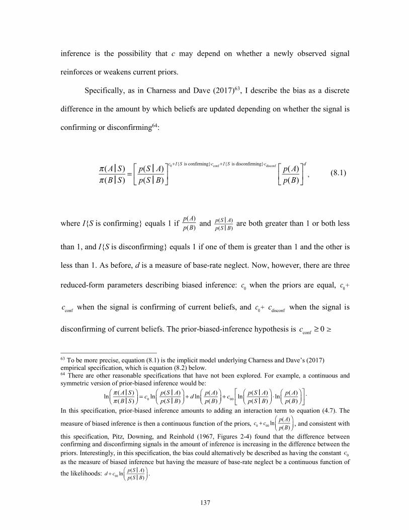
137

inference is the possibility that c may depend on whether a newly observed signal

reinforces or weakens current priors.

Specifically, as in Charness and Dave (2017)63, I describe the bias as a discrete

difference in the amount by which beliefs are updated depending on whether the signal is

confirming or disconfirming64:

, (8.1)

where I{S is confirming} equals 1 if and are both greater than 1 or both less

than 1, and I{S is disconfirming} equals 1 if one of them is greater than 1 and the other is

less than 1. As before, d is a measure of base-rate neglect. Now, however, there are three

reduced-form parameters describing biased inference: when the priors are equal, +

when the signal is confirming of current beliefs, and + when the signal is

disconfirming of current beliefs. The prior-biased-inference hypothesis is

63 To be more precise, equation (8.1) is the implicit model underlying Charness and Dave’s (2017) empirical specification, which is equation (8.2) below. 64 There are other reasonable specifications that have not been explored. For example, a continuous and symmetric version of prior-biased inference would be:

.

In this specification, prior-biased inference amounts to adding an interaction term to equation (4.7). The

measure of biased inference is then a continuous function of the priors, , and consistent with

this specification, Pitz, Downing, and Reinhold (1967, Figures 2-4) found that the difference between confirming and disconfirming signals in the amount of inference is increasing in the difference between the priors. Interestingly, in this specification, the bias could alternatively be described as having the constant as the measure of biased inference but having the measure of base-rate neglect be a continuous function of

the likelihoods: .

π (AɈS)π (B ɈS)

= p(S Ɉ A)p(S Ɉ B)

⎡

⎣⎢

⎤

⎦⎥

c0+ I{S is confirming}⋅cconf + I{S is disconfirming}⋅cdisconf p(A)p(B)

⎡

⎣⎢

⎤

⎦⎥

d

p(A)p(B)

p(S Ɉ A)p(S Ɉ B)

c0 c0

cconf c0 cdisconf

cconf ≥ 0 ≥

ln π (AɈS)π (B ɈS)

⎛⎝⎜

⎞⎠⎟= c0 ln

p(S Ɉ A)p(S Ɉ B)

⎛⎝⎜

⎞⎠⎟+ d ln p(A)

p(B)⎛⎝⎜

⎞⎠⎟+ c00 ln

p(S Ɉ A)p(S Ɉ B)

⎛⎝⎜

⎞⎠⎟⋅ ln p(A)

p(B)⎛⎝⎜

⎞⎠⎟

⎡

⎣⎢

⎤

⎦⎥

c0 + c00 lnp(A)p(B)

⎛⎝⎜

⎞⎠⎟

c0

d + c00 lnp(S Ɉ A)p(S Ɉ B)

⎛⎝⎜

⎞⎠⎟

138

, with at least one inequality strict.

In the literature, the term “confirmation bias” is sometimes used to mean the

opposite of base-rate neglect: . However, the evidence reviewed in Sections 4 and 6

indicate that base-rate neglect ( ) is the general direction of bias (Stylized Fact 1).

With prior-biased inference defined as in equation (8.1), it is separately identifiable from

base-rate neglect, and the two biases can coexist. What I call prior-biased inference is

identified by the asymmetric response to signals that confirm versus disconfirm current

priors.

Although conceptually distinct in my formulation, prior-biased inference and base-

rate neglect will often push in opposite directions in a particular updating problem because

prior-biased inference tends to reinforce an agent’s current beliefs, while base-rate neglect

will often move an agent’s beliefs away from certainty (for further discussion, see Section

10.A). Moreover, despite the general tendency for people to underinfer (Stylized Fact 7),

if , then prior-biased inference would cause people to overinfer when they

receive confirming signals.

8.B. Evidence and Models

The evidence usually adduced for confirmation bias comes from belief polarization

experiments, in which the beliefs of people with different priors who observe the same

mixed signals are typically found to move further apart. In a classic experiment, Lord,

Ross, and Lepper (1979) recruited 24 proponents and 24 opponents of capital punishment

to be experimental participants (selected based on how they had filled out an in-class

political questionnaire). The participants read a brief summary of a study that either found

cdisconf

d >1

d <1

c0 + cconf >1

139

evidence in favor of capital punishment as a deterrent or found opposite evidence. The

participants were then asked to report the change in their attitudes. Next, the participants

read a detailed account of the study. The change in their attitudes was again elicited, and

they were also asked to judge the quality and convincingness of the study. After reading

the brief summary, which did little more than provide an unambiguous statement of the

study’s conclusion, proponents and opponents both reported that their attitudes moved in

the direction of the study’s conclusion. In contrast, after participants read the detailed

account, which included information about the study’s procedures, criticisms of the study,

and rebuttals to the criticisms, participants whose prior beliefs disagreed with the

conclusion reverted to their prior beliefs. Moreover, participants whose prior attitudes

agreed with the study’s conclusion judged the study to be valid and convincing, while those

whose prior beliefs disagreed with the conclusion highlighted flaws and alternative

explanations. Finally, after participants read the detailed accounts of both the pro- and anti-

capital punishment studies, belief polarization occurred, with both proponents and

opponents reporting that their attitudes had become more extreme but in opposite

directions.

This belief-polarization effect has been replicated across a range of contexts,

including political beliefs such as the causes of climate change (Fryer, Harms, and Jackson,

2017), interpersonal beliefs such as a person’s level of academic skills (Darley and Gross,

1983), and consumer beliefs about brand quality (Russo, Meloy, and Medvec, 1998).

Reviews of the literature that are critical (e.g., Miller et al., 1993; Gerber and Green, 1999)

have highlighted that the effect is not always found, and when it is, it shows up when

140

participants’ changes in beliefs are elicited but not when the before and after levels of their

beliefs are elicited and compared.

Belief polarization is often interpreted as evidence of a bias relative to Bayesian

updating. In particular, as Lord, Ross, and Lepper (1979) argued informally, while it is not

an error for people to infer that a study that aligns with their priors is higher quality, it is

an error when people go on to use their prior-influenced assessment of the study to update

their prior in opposite directions.65 Baliga, Hanany, and Klibanoff (2013) formally proved

that agents cannot update in opposite directions in a simple Bayesian model, but they

showed that polarization can occur if agents are ambiguity averse. Moreover, a number of

researchers have shown that belief polarization can be consistent with Bayesian reasoning

in richer models (e.g., Dixit and Weibull, 2007; Andreoni and Mylovanov, 2012; Jern,

Chang, and Kemp, 2014; Benoît and Dubra, 2018). For instance, Benoît and Dubra (2018)

showed how belief polarization can occur when people have private information about an

“ancillary matter” that does not have direct bearing on the issue of interest but matters for

the interpretation of evidence. To give a concrete example, in the Lord, Ross, and Lepper

experiment, this ancillary matter might be the proposition that studies reaching right-wing

conclusions tend to be politically motivated and less intellectually honest. People who

believe that proposition are more likely to have discounted evidence in favor of capital

punishment as a deterrent in the past and are therefore more likely to enter the experiment

as an opponent of capital punishment. They are also more likely to discount the evidence

in favor of capital punishment as a deterrent during the experiment. If both proponents and

65 Fryer, Harms, and Jackson (2017) formalize this error of “two-step updating” described by Lord, Ross, and Lepper.

141

opponents of capital punishment update their priors when reading the study that confirms

their views but discount the evidence from the other study, then their beliefs will polarize.66

At the cost of being more abstract than the belief-polarization experiments,

sequential bookbag-and-poker-chip experiments provide cleaner evidence for prior-biased

inference. These experiments rule out many alternative explanations by studying fully

specified updating problems; for example, they leave little room for unobserved “ancillary

matters.” However, confirmation bias is generally thought to be stronger when people

observe ambiguous data that could be interpreted as either consistent or inconsistent with

the currently favored hypothesis (Nickerson, 1998). To the extent that the data in bookbag-

and-poker-chip experiments is unambiguous, such experiments may understate the

magnitude of prior-biased inference that may occur when the information content of signals

is more subject to interpretation.

In the earliest bookbag-and-poker-chip experiment that directly investigated prior-

biased inference, Pitz, Downing, and Reinhold (1967) posed updating problems like those

described in Section 4.C. The prior probabilities of the two states, A and B, were equal.

The probability of a signal matching the state, , was known to participants and equal to

0.6, 0.7, or 0.8. Ten participants saw chunks of N = 5 signals at a time, ten saw chunks of

N = 10 signals, and ten saw chunks of N = 20 signals. Consistent with the evidence

reviewed in Section 4.B, underinference was greater when the sample size of signals was

larger (larger N) and when the signals were more discriminable (larger ). Moreover—

66 Some of the subsequent experiments are cleaner than the Lord, Ross, and Lepper experiment because the prior is randomly assigned. For example, in Darley and Gross’s (1983) experiment, before watching a video of a nine-year-old girl and rating her academic skills, participants were either told that her family was of high or low socioeconomic status. As Rabin and Schrag (1999) noted, such a design rules out non-common priors as a possible explanation for belief polarization.

θ

θ

142

consistent with prior-biased inference—Pitz, Downing, and Reinhold found less

underinference when the signals confirmed the currently favored hypothesis. When they

examined individual-level updating, Pitz, Downing, and Reinhold found that, following a

single disconfirming signal, many participants revised their beliefs as if they had observed

a confirming signal or did not revise their beliefs at all. In sequential-updating experiments

in which participants updated after a single signal at a time, Geller and Pitz (1968) and Pitz

(1969) replicated these findings, but in two experiments with normally distributed signals,

DuCharme and Peterson (1968) found the opposite (i.e., stronger inference in response to

a disconfirming signal).

In sequential updating experiments that begin with equal priors on the two states,

prior-biased inference predicts that signals observed early on will have a greater impact on

final beliefs than signals observed later: the early signals will move the priors to assign

higher probability to one of the states, and then subsequent updating will be biased in favor

of that state. As mentioned in Section 4.C, such “primacy effects” have indeed been found

in most sequential-sample experiments that tested for them (Stylized Fact 10).

Three sequential updating experiments in the economics literature have reported

tests for prior-biased inference. One of these experiments found evidence of it (Charness

and Dave, 2017) and two did not (Eil and Rao, 2011; Möbius, Niederle, Niehaus, and

Rosenblat, 2014), but none found the opposite.67

67 Across the experiments in this literature, there are several regularities that may be related to prior-biased updating but which I do not discuss because I do not know how to interpret these regularities. For example, Pitz, Downing, and Reinhold (1967), Shanteau (1972), and Buser, Gerhards, and van der Weele (2018) found that, fixing the diagnosticity of the signal , the absolute change in beliefs (in units of probability) when updating does not depend on the priors. As another example, Coutts (2017) found a kind of primacy effect in which signals observed more frequently in the past were weighted more heavily when observed subsequently.

θ

143

In Charness and Dave’s (2017) experiment, the prior probabilities of the two states

were equal, and the probability of a signal matching the state was = 0.7. Each participant

observed six signals sequentially and, after each signal, recorded his subjective probability

of the states. Participants were incentivized for accuracy. Charness and Dave’s regression

equation is based on the logarithm of equation (8.1)68:

,

(8.2)

where equals 1 if and are both greater than 1 or

both less than 1, and equals 1 if one of them is greater than 1 and the

other is less than 1.

Charness and Dave estimated both and to be less than one, consistent with

underinference and base-rate neglect in updating problems that start from equal priors (as

per Stylized Fact 9). Moreover, they estimated and , consistent with prior-

biased inference. Charness and Dave also found that , meaning that their

68 Charness and Dave parameterized the regression slightly differently, replacing ln with a dummy

taking the value 1 if the tth signal is a and -1 if the tth signal is b. This specification is equivalent to equation (8.2), but the coefficients , , and in equation (8.2) need to be multiplied by 0.847 in order to equal the corresponding coefficients in Charness and Dave’s specification.

θ

lnπ (AɈ s1,s2 ,…,st )π (B Ɉ s1,s2 ,…,st )

⎛

⎝⎜⎞

⎠⎟

= β0 + β1 lnp(st Ɉ A)p(st Ɉ B)

⎛

⎝⎜⎞

⎠⎟+ β2 ln

π (AɈ s1,s2 ,…,st−1)π (B Ɉ s1,s2 ,…,st−1)

⎛

⎝⎜⎞

⎠⎟

+β3I{st is confirming} + β4I{st is disconfirming}+ ηt

I{st is confirming}π (AɈ s1,s2 ,…,st−1)π (B Ɉ s1,s2 ,…,st−1)

p(st Ɉ A)p(st Ɉ B)

I{st is disconfirming}

β1 β2

β3 > 0 β4 < 0

β1 + β3 >1

p(st Ɉ A)p(st Ɉ B)

⎛

⎝⎜⎞

⎠⎟

β1 β3 β4

144

experimental participants overinferred when a confirming signal was observed. Although

Pitz, Downing, and Reinhold (1967) did not report estimates from regression equation

(8.2), their experimental participants often overinferred after a confirming signal in

updating problems with low diagnosticity ( ) and extreme priors, but underinferred

after a confirming signal in updating problems with high diagnosticity ( 0.7 or 0.8) or

nearly equal priors.

What explains the prior-biased inference that has been observed in bookbag-and-

poker-chip experiments? Fischhoff and Beyth-Marom (1983, pp. 247-248) proposed that,

rather than correctly using the likelihood ratio to draw inferences, people assess how

consistent the signal is with the hypothesis they are testing—which is generally the

currently favored hypothesis—and do not take into account its consistency with other

hypotheses. That proposal dovetails nicely with Pitz, Downing, and Reinhold’s (1967, p.

391) suggestion that participants may “not perceive isolated disconfirming events as being,

in fact, contradictory to their favored hypothesis. For example, if they are fairly certain that

the 80 per cent red bag is being used, a single occurrence of a blue chip will not be

unexpected, and consequently may not lead to a decrement in subjective certainty.”

Fischhoff and Beyth-Marom argued that this bias of ignoring alternative hypotheses helps

explain a variety of other observations. For example, when psychics offer universally valid

personality descriptions, people are often impressed by how well it fits them without regard

to the fact that it would fit others equally well. As discussed in Section 7.B, Griffin and

Tversky (1992) subsequently argued that this same bias explains why people underinfer by

more in bookbag-and-poker-chip experiments when the signal rates are further apart

(Stylized Fact 6).

θ = 0.6

θ =

145

Second, Pitz, Downing, and Reinhold (p. 391) speculated that prior-biased

inference may arise because participants are unwilling to report a decrease in confidence

once they have “committed” to supporting one state as more likely. As a test of this

hypothesis, Pitz (1969) conducted a sequential bookbag-and-poker-chip experiment in

which he manipulated the salience of the participants’ posterior after the last signal when

reporting their next posterior. He found prior-biased updating when participants reported

posteriors after each signal and their posterior after the previous signal was visually

displayed, but prior-biased updating was almost completely eliminated when the previous

posterior was not displayed or when participants reported posteriors only at the end of a

sequence of signals. However, a contrary result was found in another bookbag-and-poker-

chip experiment (Beach and Wise, 1969): participants who reported beliefs after each

signal ended up with virtually the same posteriors as participants who reported beliefs only

after a sequence of signals. In a formal model related to the commitment hypothesis, Yariv

(2005) assumed that an agent has a preference for consistency and can choose her beliefs.

She showed that when the observed signal confirms the agent’s prior, the agent may choose

posteriors that are overconfident.

Eil and Rao (2011) proposed another hypothesis to explain prior-biased updating:

people want their guesses to be correct, so they view confirming evidence as “good news”

and update more strongly in response to good news than bad news. However, this

hypothesis presupposes that preference-biased inference occurs, but as discussed in the

next section, the evidence on preference-biased inference taken as a whole is not

straightforward to interpret.

146

Rabin and Schrag (1999) proposed a formal model of what they call “confirmatory

bias” in order to study the implications of prior-biased updating. The central assumption is

that the agent sometimes misperceives disconfirming signals as confirming. This

assumption is meant to capture many of the psychological mechanisms that may underlie

confirmation bias. While misperception seems implausible as a literal description of the

psychology underlying prior-biased inference in bookbag-and-poker-chips experiments, it

actually fits nicely with the evidence that experimental participants sometimes update in

the wrong direction in response to disconfirming signals, although it cannot explain the

evidence of overinference from confirming signals mentioned above.

Formally, the agent begins with equal priors on the two states A and B and observes

a sequence of i.i.d. signals, , where the signal matches the state with probability

and does not match with probability . If the agent’s priors are equal, or if she

observes a signal that matches the state that she currently thinks is more likely, then her

perceived signal is equal to the true signal . However, if she observes a signal that does

not match the state favored by her current priors, then with probability q > 0 she

misperceives the disconfirming signal to be a confirming signal. The agent is unaware that

she misperceives signals. She updates using Bayes’ Rule but using the perceived signals

instead of the true signals.

Rabin and Schrag drew out several main implications of the model. First, relative

to a Bayesian who observed the same number of a and b signals, the agent on average will

have overconfident beliefs. That is because the agent is likely to have misperceived some

disconfirming signals as confirming her current beliefs, causing her to believe more

strongly than she should in her currently favored hypothesis.

st ∈ a,b{ }

θ > 12

1−θ

st

147

Second and surprisingly, if a Bayesian observer sees that a sufficiently biased agent

believes that one state, say A, is more likely despite having perceived a sufficiently mixed

set of signals, then the Bayesian observer may conclude that the other state is in fact more

likely. The reason is that some of the signals that the agent perceived as a signals were

likely to have been b signals, which in turn means that b signals were likely the majority.

This implication, while striking, inherently applies to a scenario that is very unlikely

because it requires that the signals are highly informative ( close to 1), in which case the

sample perceived by the agent is unlikely to be sufficiently mixed.

Third, if the bias is sufficiently severe or the signals are sufficiently uninformative

( close to ½), then when observing an infinite sequence of signals, there is positive

probability that the agent will converge to certainty on belief in the wrong state. That is

because once the agent starts believing in the wrong state, confirmatory bias is likely to

cause her to perceive subsequent signals as continually building support for that hypothesis.

Pouget, Sauvagnat, and Villeneuve (2017) examined the implications of Rabin and

Schrag’s model in financial markets, assuming that some fraction of traders are rational

and some fraction have confirmatory bias. They showed that the model can explain three

well-known observations. First, excess volume arises simply because rational and biased

traders disagree and are therefore willing to trade. Second, excess volatility occurs because

the biased traders are too optimistic following an initial positive signal and too pessimistic

following an initial negative signal. Third, momentum arises and bubbles occur because

once biased traders are optimistic, they underreact to negative signals, so future prices are

expected to be higher than current prices. Pouget, Sauvagnat, and Villeneuve also derived

some novel predictions of the model: differences of opinion among traders are larger

θ

θ

148

following a sequence of mixed signals; traders are less likely to update their beliefs in the

same direction as the current signal when previous signals have pointed in the opposite

direction; and traders are less likely to update their beliefs in the same direction as the

current signal when previous belief changes have been in the opposite direction. They

found evidence consistent with these predictions using quarterly earnings surprises as a

proxy for signals, dispersion in analysts’ earnings forecasts as a proxy for differences of

opinion, and analysts’ revisions of annual earnings as a measure of beliefs updating.

149

Section 9. Preference-Biased Inference

This section discusses another potential inference bias, which I call preference-

biased inference: when people receive “good news” (i.e., information that increases

expected utility), they update more than when they receive “bad news.” In the literature,

this bias has been referred to as asymmetric updating (Möbius, Niederle, Niehaus, and

Rosenblat, 2014) or the good news-bad news effect (Eil and Rao, 2011). Almost all of the

research on this bias has been relatively recent. Preference-biased inference is a possible

mechanism underlying a bias toward optimistic beliefs.

My focus on biased inference from signals that have been observed is (again)

narrow relative to a broader literature in psychology and behavioral economics related to a

range of psychological processes that can cause beliefs to become optimistic, such as

strategic ignorance (avoiding information sources that may reveal bad news; see Golman,

Hagmann, and Loewenstein, 2017, for a review) and self-signaling (taking actions that one

later interprets as impartially revealing good news; e.g., Quattrone and Tversky, 1984;

Bodner and Prelec, 2003; Bénabou and Tirole, 2011). There is evidence for several such

processes. For example, strongly pointing to strategic ignorance, many people at risk for

Huntington’s disease refuse to be tested even though the test is inexpensive and accurate

(Oster, Shoulson, and Dorsey 2013), and similarly for HSV (Ganguly and Tasoff, 2016).

9.A. Conceptual Framework

To be precise about preference-biased inference, I once again elaborate on the

reduced-form empirical model from Section 4.A, equation (4.6):

150

.

In preference-biased inference, people draw stronger inferences—i.e., c is larger—

in response to a signal that favors the state that they prefer. Without loss of generality,

suppose expected utility in state A, denoted , is at least as large as expected utility in

state B, denoted . Following Möbius, Niederle, Niehaus, and Rosenblat (2014), I

describe the bias as a discrete difference in the amount by which beliefs are updated

depending on whether the signal is good news or bad news:

, (9.1)

where equals 1 if S = a and , equals 1 if S =

b and , and both indicators equal 0 if #$ = #&. As always, d is a measure of base-

rate neglect, but now there are three reduced-form parameters describing biased inference:

' is the same biased-inference measure discussed in Section 4, which alone governs the

bias if the agent has no preference between states; is the measure of biased

inference in response to good news; and is the measure of biased inference in

response to bad news. The preference-biased-inference hypothesis is .

Note that this specification of the preference-biased-inference hypothesis does not

require that or ; it is conceivable that having “valenced” signals (i.e., that

π (AɈS)π (B ɈS)

= p(S Ɉ A)p(S Ɉ B)

⎡

⎣⎢

⎤

⎦⎥

cp(A)p(B)

⎡

⎣⎢

⎤

⎦⎥

d

UA

UB

π (AɈS)π (B ɈS)

= p(S Ɉ A)p(S Ɉ B)

⎡

⎣⎢

⎤

⎦⎥

c0+ I{S is good news}⋅cgood+ I{S is bad news}⋅cbad p(A)p(B)

⎡

⎣⎢

⎤

⎦⎥

d

I{S is good news} UA >UB I{S is bad news}

UA >UB

c + cgood

c + cbad

cgood > cbad

cgood ≥ 0 cbad ≤ 0

151

are good or bad news) could affect the overall amount of underinference or overinference

relative to having unvalenced signals.

9.B. Evidence and Models

In one of the pioneering papers on preference-biased inference69, Möbius, Niederle,

Niehaus, and Rosenblat (2014) argued that it may arise as an “optimal bias” for agents who

get utility directly from holding optimistic beliefs. In Möbius et al.’s model, which builds

on the theoretical framework from Brunnermeier and Parker (2005), agents can choose ex

ante (i.e., before observing any signals) the weight they put on the likelihood ratio—the

value of c in equation (4.6)—for each possible signal they might observe. The benefit of

deviating from Bayesian updating is that beliefs can end up being more optimistic, but the

cost is that biased beliefs can lead to suboptimal behavior. In the model, the agent optimally

chooses to weight bad news less than good news. Moreover, to offset the increased risk of

suboptimal behavior, the agent optimally chooses to underweight the likelihood ratio for

all signals. Thus, the agent has conservatism bias (as in Section 5.B) but is more

conservative in response to bad news than good news. Bénabou (2013) proposed a model

in which an agent can choose whether or not to process a signal that has been observed

(i.e., to not pay attention to it, explain it away, or not think about it); if the agent gets

anticipatory utility from putting high probability on the good state, then the agent may

selectively ignore bad news.

In the economics literature, the evidence regarding preference-biased inference

comes from sequential-updating experiments, in which participants are updating about a

69 All results from Möbius et al. are from the most recent, 2014 working paper, but the original working paper is from 2007.

152

preference-relevant event. Möbius at al. conducted one of the earliest such experiments.

Each participant took an IQ test. The two states of the world are A = {scored in top half of

the IQ test} and B = {scored in bottom half}. Participants’ beliefs were measured both

before and after the IQ test and then again after each of four, independent binary signals.

Each signal matched the true state with probability = 0.75. The belief elicitation was

incentive compatible.

Möbius et al. estimated a regression equation corresponding to the logarithm of

equation (9.1) above:

(9.2)

In terms of equation (9.1), gives an estimate of , gives an estimate of c +

, and gives an estimate of the base-rate neglect parameter d. Möbius et al. found

(SE = 0.01) and (SE = 0.03).70 Both are less than one, indicating

underinference in response to both good and bad news. Moreover, the estimates imply

, consistent with preference-biased inference.

70 For the coefficient on the prior ratio, Möbius et al. estimate = 0.98 (SE = 0.06). Since this coefficient is essentially one, it indicates that there is no base-rate neglect in Möbius et al.’s data. As discussed in Section 4.C, most sequential-sample experiments find stronger evidence of base-rate neglect.

θ

lnπ (AɈ s1,s2 ,…,st )π (B Ɉ s1,s2 ,…,st )

⎛

⎝⎜⎞

⎠⎟

= δ1I st = a{ }ln p(st Ɉ A)p(st Ɉ B)

⎛

⎝⎜⎞

⎠⎟+δ 2I st = b{ }ln p(st Ɉ A)

p(st Ɉ B)⎛

⎝⎜⎞

⎠⎟

+δ3 lnπ (AɈ s1,s2 ,…,st−1)π (B Ɉ s1,s2 ,…,st−1)

⎛

⎝⎜⎞

⎠⎟+ζ t ,

δ1 c + cgood δ 2

cbad δ3

δ1 = 0.27 δ 2 = 0.17

cgood > cbad

δ3

153

Experiments on preference-biased inference typically include a control condition

in which participants are updating about an event that is not preference-relevant. In Möbius

et al.’s control condition, participants repeated the updating task, except with reference to

the performance of a robot rather than their own performance. The robot’s initial

probability of being a high type was set equal to the multiple of 0.05 closest to the

participant’s post-IQ-test belief about herself. That way, the state of the world about which

the participant was updating had essentially the same prior probability and differed only in

not being preference-relevant. In this control condition, Möbius et al. found less

underinference overall and no asymmetry.71

While Möbius et al. found that bad news was underweighted by more than good

news, the evidence from similar experiments taken as a whole is mixed. Three papers have

found stronger inference from good news: Möbius et al. (2014), Eil and Rao (2011), and

Charness and Dave (2017). The opposite result—stronger inference from bad news—was

found in three papers: Ertac (2011) and Coutts (2017), as well as by Kuhnen (2015) for

outcomes that take place in the loss domain (but not those that take place in the gain

domain). Five papers have tested and found no evidence for asymmetry: Grossman and

Owens (2012), Buser, Gerhards, and Van der Weele (2016), Schwardmann and Van der

Weele (2016), Barron (2016), and Gotthard-Real (2017). Note also that while Eil and Rao

(2011) found stronger inference from good news for participants’ beliefs about their own

beauty, they found no evidence for asymmetry for participants’ beliefs about their own IQ.

71 This is the result with their preferred sample restrictions, including only participants who updated at least once in the correct direction and never in the wrong direction (their Table 4 Column I). In the full sample, the amount of underinference is stronger overall and asymmetric, with greater updating in response to a signals (their Table 4 Column III).

154

There does not appear to be a neat explanation for the puzzling differences in results

across experiments. Coutts (2017) suggested that since the experiments differ in the prior

probability of state A, what appears to be preference-biased inference might actually be

driven by prior-biased inference. However, Möbius et al. (2014) and Eil and Rao (2011)

found evidence for preference-biased inference despite not finding prior-biased inference.

Moreover, three papers tested for preference-biased inference with controls for priors or

for prior-biased inference (Schwardmann and Van der Weele, 2016; Charness and Dave,

2017; Coutts, 2017) and reached different conclusions about the presence and direction of

preference-biased inference.72

Another hypothesis is that different results across experiments may arise from

differences in signal structure, which varies a great deal across the experiments. For

example, different from Möbius et al. (2014), Ertac (2011) elicited participants’

probabilities of scoring in the top, middle, or bottom tercile on a math quiz, and then

provided a perfectly informative signal that performance is top/not-top or bottom/not-

bottom. However, there are opposite results even across experiments with similar signal

structures. For instance, Coutts’s (2017) design is similar to Möbius et al.’s (2014), except

with instead of 0.75.

In parallel with the economics literature on preference-biased inference, there is a

literature in psychology and neuroscience based on a different experimental design. In the

pioneering experiment, Sharot, Korn, and Dolan (2011) presented participants with 80

72 As noted at the end of Section 8.B, Eil and Rao (2011) hypothesized the opposite: that what appears to be evidence for prior-biased inference may actually be due to preference-biased inference, if people consider prior-supporting signals to be good news. Consistent with this hypothesis, Eil and Rao found little evidence of prior-biased inference when separately examining updating in response to signals that are good versus bad news, but the data are quite noisy. Their intriguing hypothesis does not appear to have been tested in other papers. However, the mixed overall evidence regarding preference-biased inference, combined with the relatively stronger evidence overall regarding prior-biased inference, leans against this hypothesis.

θ = 0.67

155

randomly ordered short descriptions of negative life events, such as having one’s car stolen

or having Parkinson’s disease. Participants were asked the likelihood of the event

happening to them (without incentives for accuracy). Participants were then shown the

population base rate of the event, and their belief was re-elicited. “Good news” is defined

as learning that the base rate is lower than the participant’s initial probability. Almost all

of the experiments in this literature find that the absolute change in participants’

probabilities is larger in response to good news than bad news.73

Wiswall and Zafar (2015) reported a related study as part of a broader field

experiment on the effects of providing information about earnings on students’ beliefs and

choices of undergraduate major. They provided 240 students with mean earnings of age-

30 individuals and 255 students with the same information broken down by college major.

Pooling across the two groups, they found that the information caused students who learned

that they had overestimated population earnings to revise their own expected earnings

downward by $159 per $1,000, while those who had underestimated earnings revised

upward by $347 per $1,000. As Wiswall and Zafar highlight, however, the difference is far

from statistically distinguishable, with a p-value of 0.327.

These experiments, however, have a design limitation: because receipt of good

news versus bad news is not randomly assigned—whether the news is good or bad depends

on one’s prior belief—those who receive good news about a particular event may differ on

unobservables from those who receive bad news. For example, those who are more

73 The experiments finding such asymmetric updating include Sharot, Guitart-Masip, et al. (2012), Sharot, Kanai, et al. (2012), Moutsiana et al. (2013), Chowdhury et al. (2014), Garrett and Sharot (2017), Garrett et al. (2014), Korn et al. (2014), Kuzmanovic, Jefferson, and Vogeley (2015, 2016), and Krieger, Murray, Roberts, and Green (2016). An exception is Shah et al. (2016), who argued that the findings of asymmetry are due to a variety of methodological limitations with this kind of study design. Garrett and Sharot (2017), however, argued that the original findings are robust to addressing these limitations.

156

optimistic about an event may also be more confident about it and therefore update less in

response to news. (The bookbag-and-poker-chip experiments discussed above eliminate

such confounds by randomly assigning good and bad news.) Wiswall and Zafar partially

addressed such a potential confound by testing whether any asymmetric response to good

news versus bad news is associated with demographics they measured, and they found no

evidence for such correlation.

Beginning with Kuzmanovic, Jefferson, and Vogeley (2015), some recent work in

psychology and neuroscience overcomes this limitation by randomly assigning bogus base-

rate information (e.g., Marks and Baines, 2017).74 For example, Kuzmanovic et al.

followed the same basic design as Sharot et al.—eliciting the participant’s belief about

likelihood of an event, providing the population base rate, and then re-eliciting the

participant’s belief—but told the participant that the population base rate is equal to the

participant’s belief plus or minus a random number. These experiments confirm the finding

from the earlier studies that participants update more in response to good news than bad

news.75

Taken all together, the evidence on preference-biased inference is confusing. In the

economics literature, there are many bookbag-and-poker-chip experiments that reach

74 Within experimental economics, providing bogus information is viewed as deceptive, and deceiving experimental participants is generally considered unacceptable (or at least unethical), especially if non-deceptive methods could be used instead. A non-deceptive method of randomizing the numbers provided to participants would be to show them actual numbers obtained from different sources (as was done in a different context by Cavallo, Cruces, and Perez-Truglia, 2016). 75 A related strand of work in psychology and neuroscience conducts two-armed bandit experiments. In each round, participants can receive a payoff from either of two bandits, which give rewards at different, unknown rates. The rate of reinforcement learning is estimated separately in response to better-than-expected outcomes and worse-than-expected outcomes (i.e., positive and negative reward prediction errors). Lefebvre et al. (2017) found that experimental participants learn at a higher rate from better-than-expected outcomes. Palminteri et al. (2017) replicated this finding but also found that when the counterfactual payoffs from the unchosen bandit is also revealed in each round, then for these counterfactual payoffs, participants learn at a higher rate from worse-than-expected outcomes. Palminteri et al. interpreted their result as consistent with prior-biased inference: people update more in response to information that confirms their current choice.

157

opposite conclusions, and there the obvious candidate explanations for the differences in

findings do not seem to be right. In the psychology and neuroscience literature, the

experiments are based on a different design, and the results are nearly unanimous in finding

evidence in favor of preference-biased inference. Sorting out the reasons why different

experiments reach different conclusions should be a priority.

158

Section 10. Discussion

This chapter has reviewed a range of belief biases. In this final section, I comment

on some interrelated, overarching issues that relate to many of the biases and to the

literature as a whole.

10.A. When Do People Update Too Much or Too Little?

Do people update too much or too little, relative to Bayesian updating? The

predominant view in the literature has shifted over time. The early literature focused

exclusively on conservatism bias and characterized people as generally underinferring. As

mentioned in Section 7, upon first learning about this literature from Amos Tversky in

1968, Daniel Kahneman (2002) recalled thinking “The idea that people were conservative

Bayesian did not seem to fit with the everyday observation of people commonly jumping

to conclusions.” Much of Kahneman and Tversky’s work, especially on the LSN (Tversky

and Kahneman, 1971) and base-rate neglect (Kahneman and Tversky, 1982), focused on

examples of people updating too much. Enamored with the new methods and findings from

research on representativeness, psychologists lost interest in the conservatism literature and

started doubting its methods and conclusions. As Fischhoff and Beyth-Marom (1983)

summarized the general view at the time:

In the end, this line of research [on bookbag-and-poker-chip experiments]

was quietly abandoned…This cessation of activity seems to be partly due

to the discovery of the base-rate fallacy, which represents the antithesis of

conservatism and other phenomena that led researchers to conclusions such

159

as the following: “It may not be unreasonable to assume that…the

probability estimation task is too unfamiliar and complex to be meaningful”

(Pitz, Downing, and Reinhold, 1967, p. 392). “Evidence to date seems to

indicate that subjects are processing information in ways fundamentally

different from Bayesian…models” (Slovic and Lichtenstein, 1971, p. 728).

“In his evaluation of evidence, man is apparently not a conservative

Bayesian; he is not Bayesian at all” (Kahneman and Tversky, 1972a, p.

450).

My view—hopefully communicated throughout this chapter—is that whether

people update too much or too little is the wrong question. A better question is when we

may expect one versus the other.

Here is a broad-brush summary, focusing on several of the main biases reviewed in

this chapter and on the usual case of updating about state A versus B from independent

binomial signals, with a signals having probability in state A and probability

in state B. By and large, people update too little, with three exceptions. First, when

and are close together, people overinfer from signals and hence update too much

(Section 4.A). Second, people may overinfer and thus update too much due to prior-biased

updating, when the signal goes in the same direction of the priors (Section 8). Third, people

may update too much due to base-rate neglect, when the priors are extreme and the signal

goes in the opposite direction of the priors (Section 6). As noted in Section 8.A, these latter

two biases—prior-biased updating and base-rate neglect—push in opposite directions. A

plausible conjecture is that prior-biased updating dominates when the priors are close to

θ A >12

θB <

12

θ A

θB

160

50-50 whereas base-rate neglect dominates when the priors are extreme, but I am not aware

of any work that has directly examined how these two biases interact.

10.B. Modeling Challenges

Following Barberis, Shleifer, and Vishny (1998), many models of belief biases

have been what Rabin (2013) calls “quasi-Bayesian,” meaning that the agent has the wrong

model of the world but is fully Bayesian with respect to that wrong model. Of those

discussed in this chapter, only the models of the LSN (Rabin, 2002; Rabin and Vanayos,

2010) are quasi-Bayesian. The model of prior-biased updating (Rabin and Schrag, 1999) is

closely related; the agent is Bayesian but misreads some of the signals she observes. Quasi-

Bayesian and misread-signal models are attractive analytically because the standard

machinery for studying Bayesian models can be brought to bear. They are also attractive

theoretically because the agent’s beliefs are logically consistent (despite being incorrect);

as discussed below, logical inconsistencies raise thorny issues that have barely begun to be

studied.

The quasi-Bayesian and misread-signal models that have been proposed to date are

also examples of what Rabin (2013) calls “portable extensions of existing models

(PEEMs).” PEEMs are defined by two properties: (i) they embed the Bayesian model as a

special case for particular values of one or more bias parameters, and (ii) they are portable

across environments in the sense that the independent variables are the same as for existing

models. PEEMs are attractive for a number of reasons. Most relevantly for the discussion

here, once the parameters of a PEEM are pinned down by empirical estimates, the model

has no degrees of freedom beyond those that are already available in the Bayesian model.

161

The models of NBLLN (Benjamin, Rabin, and Raymond, 2016), partition

dependence (Benjamin, Moore, and Rabin, 2018), base-rate neglect (Benjamin, Bodoh-

Creed, and Rabin, 2018), and local thinking (Gennaioli and Shleifer, 2010) are neither

quasi-Bayesian models nor PEEMs. The models are not PEEMs because they fail criterion

(ii): there is an independent variable that is irrelevant for a Bayesian agent but relevant in

the model. In particular, as discussed in Sections 4.C, 5.A, and 6, for the models of NBLLN

and base-rate neglect, the grouping of signals needs to be specified in order to pin down

the model’s predictions (more generally, He and Xiao (2017) show that grouping will

matter for any non-Bayesian updating rule). For partition dependence, it is the set of bins

that is a crucial new independent variable. For the model of local thinking, as discussed in

Section 7.C, additional assumptions may be needed to apply it outside the context where it

has been formulated.

Because the models have new independent variables that must be specified in

applications, the models have degrees of freedom that the Bayesian model does not have.

In some cases, these degrees of freedom may not be a problem for studying the model in

an experiment because, by framing the judgment problem in a particular way, the

experimenter can plausibly control the new independent variables. In applied settings,

however, a researcher will often not have such control and may not observe, say, how an

agent groups the signals she observes or how she partitions the state space into bins when

formulating her beliefs.

When the degrees of freedom are left unspecified, the models are less powerful than

the Bayesian model because they rule out fewer possible observations (i.e., assumptions

can be made ex post to rationalize what was observed). To turn a non-PEEM into a PEEM,

162

additional modeling is needed to pin down the values of the free parameters as a function

of observable characteristics of the judgment problem.76 In the cases of NBLLN, partition

dependence, base-rate neglect, and local thinking, there is currently little evidence

available to guide such modeling. New experiments will be needed to provide that

evidence.

Because these models are not quasi-Bayesian, the agent’s beliefs are not internally

consistent across different framings of the same judgment problem. This is not necessarily

a problem in individual decision-making environments as long as the agent always views

the problem in the same frame, but it raises the question of what an agent would believe if

she views the same problem with different frames over time. Would the agent always use

the current frame, despite knowing that she herself had previously thought about the

problem differently?

Additional complications arise in environments with strategic interaction between

agents. Such environments often require assumptions about higher-order beliefs about

agents’ biases and framing of the judgment problem, not only what Agent 1 believes about

Agent 2 but also what Agent 1 believes Agent 2 believes about Agent 1, etc. A natural

assumption is naïveté: Agent 1 believes that other agents make the same predictions and

draw the same inferences as she does. But what if Agent 1 knows that other agents frame

the information differently (say, Agent 1 observes 20 samples of individual signals but

knows that Agent 2 observes the entire sample of 20 signals at once), or if the other agent’s

behavior is inconsistent with holding the same beliefs as Agent 1? Addressing these and

76 The same issue arises with other models in behavioral economics, for example, with the reference point in models of reference-dependent preferences. As discussed in Chapter XXX (by O’Donoghue and Sprenger), recent work on loss aversion has devoted substantial attention to understanding how the reference point for gains and losses is endogenously determined.

163

other questions requires an equilibrium concept that can accommodate belief biases.

Chapter XXX (by Eyster) of this Handbook addresses these and related issues in the

context of several errors in reasoning, but it does not study the same biases that are the

focus of this chapter. There is much fertile ground for new evidence and theory to begin to

understand how errors in probabilistic reasoning play out dynamically and in environments

with strategic interaction.

10.C. Generalizability from the Lab to the Field

Much of the evidence reviewed in this chapter has been from bookbag-and-poker-

chip experiments or similarly abstract laboratory studies. Such studies typically provide

the cleanest evidence on errors in probabilistic reasoning because the properties of the

random processes and the information provided to participants can be tightly controlled.

This control enables researchers to rule out alternative interpretations of apparent belief

biases. Yet laboratory evidence is often prone to concerns about generalizability:

laboratory behavior may give a misleading impression of how people behave in the field

settings that are of primary interest to economists. I will briefly highlight five potentially

relevant differences between the typical laboratory environment and the typical field

setting that could limit generalizability: incentives, experience, markets, populations,

problem structure, and framing.

Grether’s (1980) seminal economic experiments on errors in probabilistic

reasoning were motivated by questions of whether the biases found in psychology

experiments would also be found in settings where participants were incentivized and

experienced and where the random processes were made transparent and credible. To

164

achieve transparency and credibility, Grether (1980) adopted the bookbag-and-poker-chip

experimental design and drew balls from urns in front of participants. In addition to testing

for deviations from Bayesian updating, he also studied the robustness of these deviations

to incentives for correct answers and experience with the same updating problem. In earlier

work from psychology, there was also some attention to the effect of incentives (e.g.,

Phillips and Edwards, 1966) and experience (e.g., Martin and Gettys, 1969; Strub, 1969).

Aggregating over findings from many papers, the meta-analysis results from Section 4

suggest that, overall, the presence of incentives in bookbag-and-poker-chip experiments

does not eliminate deviations from Bayesian updating. Among papers that examine the

effect of experience, a typical finding is that it reduces but does not eliminate bias (e.g.,

Camerer, 1987). I am not aware of any systematic overview of the effects of experience.

Other groundbreaking, early economics papers in this literature addressed whether

deviations from Bayesian updating would persist in experimental asset markets and

influence market outcomes (Duh and Sunder, 1986; Camerer, 1987; Anderson and Sunder,

1995; Camerer, 1990). In general, these papers found that base-rate neglect and exact

representativeness do influence market prices, although the effects are weak and reduced

when experimental participants gain experience (for a brief review, see Camerer, 1995, pp.

605-608). The work has addressed only a few of the many relevant questions that might be

asked about markets. For example, one might conjecture that in life insurance markets,

where supply-side competition may drive prices to marginal cost (as determined by

actuarial tables), in equilibrium belief biases influence quantities rather than prices (who

buys insurance).

165

While much of the laboratory evidence on belief biases to date is from student

samples, a number of papers have examined generalizability to other populations. For

example, Dohmen, Falk, Huffman, Marklein, and Sunde (2009) found that the GF is

widespread in a representative sample from the German population. There is relatively

little evidence, however, on how the magnitude of biases compares across populations.

Since students are often found to be less biased than other, less educated, demographic

groups, it seems likely that evidence from student samples understates the prevalence and

magnitude of biases. Relevant to the question of how much bias can be expected in

particular field settings, some research has studied how individual characteristics are

correlated with biases (e.g., Stanovich and West, 1998; Stanovich, 1999). Relatedly, for

making predictions about how biases interact, it may be valuable to know how biases are

correlated with each other in the population (for some work along these lines, see, e.g.,

Stango, Yoong, and Zinman, 2017; Falk, Becker, Dohmen, Enke, Huffman, and Sunde,

2018; Chapman, Dean, Ortoleva, Snowberg, and Camerer, 2018).

A longstanding generalizability concern is related to differences in problem

structure between the lab and the field. Specifically, people’s beliefs may result from

heuristics or mental models that are well adapted to real-world problems—i.e., they do not

lead to systematic biases in naturalistic environments—but that cause biased responses in

the problems posed in the lab. For example, Winkler and Murphy (1973) argued that real-

world random processes are typically different from the i.i.d. processes in bookbag-and-

poker-chip experiments, e.g., featuring positive autocorrelation and non-stationarity. They

argued that in these real-world settings, people update correctly, but when faced with the

unfamiliar, artificial i.i.d. settings created in the lab, people behave as they would when

166

facing real-world random processes. This behavior generates underinference in i.i.d.

settings, but researchers would be mistaken to generalize that people underinfer in the field.

The force of the problem-structure critique is weakened by a lack of evidence or clear

intuition on what the relevant real-world random processes actually looks like (indeed,

while Winkler and Murphy posited positive autocorrelation of real-world random

processes in order to explain underinference, the GF is sometimes rationalized by arguing

that real-world random processes are negatively correlated.) Moreover, while experimental

participants surely do bring some expectations from their everyday experiences into the

lab, the problem-structure critique does not provide a plausible explanation for all of the

lab evidence. For example, everyone has enough experience with coin flips to understand

what the random process is when told that a fair coin is being flipped, and much of the

evidence for the GF and other biases can be (and has been) generated using coin flips.

Furthermore, if a particular version of the critique predicts that people form beliefs as if

outcomes were generated by a specific, non-i.i.d. (but internally consistent) random

process, then it cannot explain why people’s beliefs are internally inconsistent, with beliefs

depending on the question they are asked (see Section 3.F).

Another generalizability concern is that whether and how people are biased depends

on how problems are framed. Most famously, some biases are smaller in magnitude when

problems are posed in terms of frequencies rather than probabilities, and frequencies have

been argued to be more common in field settings (e.g., Tversky and Kahneman, 1983;

Gigerenzer and Hoffrage, 1995).

More generally, the cognitive processes underlying belief formation and revision,

such as perception, attention, and memory, plausibly operate differently in natural

167

environments than they do in abstract settings. For example, people may pay more attention

or process information more effectively when they are more familiar with or more

interested in the context. Some versions of this concern can be and have been studied in

the lab. For example, in a bookbag-and-poker-chip experiment with accounting students as

participants, Eger and Dickhaut (1982) found less underinference when the experiment was

framed in terms of an accounting problem rather than as an abstract problem. Yet it is not

necessarily the case that biases are smaller in more naturalistic settings; for example,

Ganguly, Kagel and Moser (2000) found that base-rate neglect was stronger in an

experimental market when it was framed in terms of buying and selling stocks than in terms

of abstract balls and urns.

All of the above evidence notwithstanding, the most compelling response to

concerns about generalizability to the field is field studies. Of the topics discussed in this

chapter, the GF, the hot-hand bias, and base-rate neglect are relatively well documented in

field settings. Most of the other biases in this chapter are in need of more field evidence.

For example, could it be that preference-biased updating powerfully influences our

political and social beliefs, even if it is difficult to reliably observe in bookbag-and-poker

experiments? For biases lacking much field evidence, I urge caution in generalizing from

abstract laboratory settings, and as discussed further in 10.E below, I advocate field studies

as a high priority.

10.D. Connecting With Other Areas of Economics

In behavioral finance, research on forecasting errors has drawn on the biases

reviewed in this chapter. In particular, the LSN, base-rate neglect, and local thinking have

168

been argued to be leading contributors to extrapolative expectations; see Chapter XXX (by

Barberis) of this Handbook.

The relevance of errors in probabilistic reasoning to economics, however, should

be far broader. Indeed, as noted at the very beginning of this chapter, belief biases could

matter for any context of decision making under risk, including portfolio choice, insurance

purchasing, and search and experimentation. Belief biases should also be crucial for

research on stereotyping and statistical discrimination, since these can be based on

erroneous beliefs (e.g., Bordalo, Coffman, Gennaioli, and Shleifer, 2016; Bohren, Imas,

and Rosenberg, 2018). Belief biases should similarly be central to the study of persuasion,

since persuaders will aim to exploit the biases of persuadees. Yet these and other areas of

economics remain virtually untouched by insights from the literature on belief biases and

are thus fertile ground for enterprising researchers.

There are at least two other literatures within economics which, to date, have

proceeded almost completely independently from the work reviewed in this chapter despite

being closely related. The first is the line of work on sticky expectations (e.g., Gabaix and

Laibson, 2002; Mankiw and Reis, 2002) and learning in macroeconomics (see, e.g., Evans

and Honkapohja, 2001). Research in macroeconomics may benefit from the accumulated

evidence and theorizing about belief biases, and behavioral economists should take on the

challenge of explaining key features of macroeconomic beliefs.

The second is the literature on survey measurement of expectations (e.g., Viscusi,

1990; Manski, 2018; Coibion, Gorodnichenko, and Kamdar, forthcoming). Sampling-

distribution biases would be especially relevant to that literature, and in particular, the

survey literature should be aware of and correct for partition dependence (Section 3.A) and

169

extreme-belief aversion (Section 5.C). Conversely, experimental research that elicits

sampling distributions would benefit from methodological advances in the survey

literature, such as modeling and adjusting for measurement error and for rounding of

numerical answers (e.g., Giustinelli, Manski, and Molinari, 2018).

10.E. Some Possible Directions For Future Research

To end this chapter, I highlight three directions for future research that seem to me

to be especially important. First, although the tradition in behavioral economics has been

to focus on one bias at a time, studying several biases at once will often be essential in

research on belief biases. Doing so may be necessary to separately identify the biases. For

example, partition dependence can be a confound for assessing other sampling-distribution

biases, biased inference is often confounded with biased use of prior information, and prior-

biased updating and preference-biased updating are often confounded with each other.

Studying biases jointly will also be important to assess the robustness of the predictions

that arise from one bias to the presence of another bias. For example, as discussed above

in Section 10.A, prior-biased updating and base-rate neglect make opposite predictions

about whether people will update too much or too little; studying the interaction between

the biases will be necessary to understand when one or the other dominates.

Second, the efforts to model belief biases have taught us that some additional

evidence is needed as an input to further modeling, and new experiments should collect

that evidence. For example, as discussed in Sections 4.C, 5.A, and 6, when modeling how

people update after observing a sequence of signals, predictions may hinge on an

assumption about how people group the signals. Few experiments to date have addressed

170

that question (with the exceptions of Shu and Wu, 2003, and Kraemer and Weber, 2004).

In many dynamic settings, another important modeling assumption is what people expect

about how their own beliefs will evolve if they observe additional signals. Similarly, in

strategic interactions, a key assumption is what people believe about how others’ beliefs

will evolve. Evidence is needed to inform those assumptions, as well.

Finally, the vast majority of evidence on belief biases comes from laboratory

studies; more field evidence is needed to probe generalizability (as discussed in Section

10.C) and to assess the economic importance of the biases. Most existing field evidence is

from gambling (e.g., Metzger, 1985), lotteries (e.g., Clotfelter and Cook, 1993), and sports

(e.g., Gilovich, Vallone, and Tversky, 1985), environments where the true probabilities are

known or can be reliably estimated and where data have long been publicly available.

However, recent work has begun to examine other settings. For example, Chen,

Moskowitz, and Shue (2016) studied reviews of loan applications and judges’ decisions in

refugee asylum court (in addition to umpires’ calls on baseball pitches), and Augenblick

and Rabin (2018) studied how beliefs evolve over time in prediction markets. As has

occurred with other areas of behavioral economics, once it becomes clear that errors in

probabilistic reasoning matter in a range of economically relevant field settings, this area

of research will become part of mainstream economics.

171

172

References Ahn, D.S., Ergin, H., 2010. Framing Contingencies. Econometrica, 78 (2), 655–695. Alberoni, F., 1962a. Contribution to the Study of Subjective Probability. I. The Journal of

General Psychology, 66 (2), 241-264. Alberoni, F., 1962b. Contribution to the Study of Subjective Probability: Prediction. II.

The Journal of General Psychology, 66 (2), 265-285 Alesina, A., Miano, A., Stantcheva, S., 2018. Immigration and Redistribution. Working

Paper. Ambuehl, S., Li, S., 2018. Belief updating and the demand for information. Games and

Economic Behavior, 109, 21-39. Anderson, M.J., Sunder, S., 1995. Professional Traders as Intuitive Bayesians.

Organizational Behavior and Human Decision Processes, 64 (2), 185-202. Andreoni, J., Mylovanov, T., 2012. Diverging Opinions. American Economic Journal:

Microeconomics, 4 (1), 209-232. Anobile, G., Cicchini, G.M., Burr, D.C., 2016. Number As a Primary Perceptual Attribute:

A Review. Perception, 45 (1-2), 5-31. Antoniou, C., Harrison, G.W., Lau, M.I., Read, D., 2013. Revealed Preference and the

Strength/Weight Hypothesis. Warwick Business School, Finance Group. Antoniou, C., Harrison, G.W., Lau, M.I., Read, D., 2015. Subjective Bayesian beliefs.

Journal of Risk and Uncertainty, 50 (1), 35-54. Arnold, D., Dobbie, W., Yang, C.S., Forthcoming. Racial Bias in Bail Decisions. The

Quarterly Journal of Economics. Asparouhova, E., Hertzel, M., Lemmon, M., 2009. Inference from Streaks in Random

Outcomes: Experimental Evidence on Beliefs in Regime Shifting and the Law of Small Numbers. American Management Science, 55 (11), 1766-1782.

Augenblick, N., Rabin, M., 2018. Belief Movement, Uncertainty Reduction, & Rational Updating. Working Paper.

Avugos, S., Bar-Eli, M., Ritov, I., Sher, E., 2013.The elusive reality of efficacy performance cycles in basketball shooting: analysis of players' performance under invariant conditions. International Journal of Sport and Exercise Psychology, 11 (2), 184-202.

Ayton, P., Fischer, I., 2004. The hot hand fallacy and the gambler’s fallacy: Two faces of subjective randomness?. Memory & Cognition, 32 (8), 1369-1378.

Bacon, F., 1620. The New Organon and Related Writings. Liberal Arts Press, New York. Baliga, S., Hanany, E., Klibanoff, P., 2013. Polarization and Ambiguity. American

Economic Review, 103 (7), 3071-3083. Bar-Eli, M., Avugos, S., Raab, M., 2006. Twenty years of “hot hand” research: Review

and critique. Psychology of Sport and Exercise, 7 (6), 525-553.

173

Bar-Hillel, M., 1979. The Role of Sample Size in Sample Evaluation. Organizational Behavior and Human Performance, 24 (2), 245-257.

Bar-Hillel, M., 1980. The base-rate fallacy in probability judgments. Acta Psychologica, 44 (3), 211-233.

Bar-Hillel, M., 1982. Studies of representativeness. In: Kahneman, D., Slovic, P., Tversky, A., (Eds.), Judgment under uncertainty: Heuristics and biases, Cambridge University Press, New York, pp. 69-83.

Barberis, N., Shleifer, A., Vishny, R., 1998. A model of investor sentiment. Journal of Financial Economics, 49 (3), 307-343.

Barbey, A.K., Sloman, S.A., 2007. Base-rate respect: From ecological rationality to dual processes. Memory & Cognition, 30 (3), 241-254.

Barron, K., 2016. Belief updating: Does the ‘good-news, bad-news’ asymmetry extend to purely financial domains?. WZB Discussion Paper, SP II 2016-309.

Bateman, I., Munro, A., Rhodes, B., Starmer, C., Sugden, R., 1997. Does Part-Whole Bias Exist? An Experimental Investigation. The Economic Journal, 107 (441), 322-332.

Beach, L.R., 1968. Probability Magnitudes and Conservative Revision of Subjective Probabilities. Journal of Experimental Psychology, 77 (1), 57-63.

Beach, L.R., Wise, J.A., 1969. Subjective Probability Revision and Subsequent Decisions. Journal of Experimental Psychology, 81 (3), 561-565.

Beach, L.R., Wise, J.A., Barclay, S., 1970. Sample Proportions and Subjective Probability Revisions. Organizational Behavior and Human Performance, 5 (2), 183-190.

Bénabou, R., 2013. Groupthink: Collective Delusions in Organizations and Markets. Review of Economic Studies, 80 (2), 429-462.

Bénabou, R., Tirole, J., 2011. Identity, Morals, and Taboos: Beliefs as Assets. The Quarterly Journal of Economics, 126 (2), 805-855.

Bénabou, R., Tirole, J., 2016. Mindful Economics: The Production, Consumption, and Value of Beliefs. Journal of Economic Perspectives, 30 (3), 141-164.

Benartzi, S., Thaler, R.H., 1999. Risk Aversion or Myopia? Choices in Repeated Gambles and Retirement Investments. Management Science, 45 (3), 346-381.

Benartzi, S., Thaler, R.H., 2001. Naïve Diversification Strategies in Defined Contribution Savings Plans. American Economic Review, 91 (1), 79-98.

Benjamin, D., Bodoh-Creed, A.L., Rabin, M., 2018. Base-Rate Neglect: Foundations and Implications. Working Paper.

Benjamin, D., Moore, D., Rabin, M., 2018. Biased Beliefs About Random Samples: Evidence from Two Integrated Experiments. Working Paper.

Benjamin, D., Rabin, M., Raymond, C., 2016. A Model of Non-Belief in the Law of Large Numbers. Journal of the European Economic Association, 14 (2), 515-544.

Benoît, J-P., Dubra, J., 2018. When do populations polarize? An explanation. Working Paper.

174

Bhargava, S., Fisman, R., 2014. Contrast Effects in Sequential Decisions: Evidence from Speed Dating. Review of Economics and Statistics, 96 (3), 444-457.

Blondé, J., Girandola, F., 2016. Revealing the elusive effects of vividness: a meta-analysis of empirical evidences assessing the effect of vividness on persuasion. Social Influence, 11 (2), 111-129.

Bodner, R., Prelec, D., 2003. Self-Signaling and Diagnostic Utility in Everyday Decision Making. In: Brocas, I., Carrillo, J.D. (Eds.), The Psychology of Economics Decisions. Vol. 1. Rationality and Well-being, Oxford University Press, New York, pp. 105-126.

Bohren, A., Imas, A., Rosenberg, M., 2018. The Dynamics of Discrimination: Theory and Evidence. Working Paper.

Bordalo, P., Gennaioli, N., Shleifer, A., 2018. Diagnostic Expectations and Credit Cycles. Journal of Finance, 73 (1), 199-227.

Bordalo, P., Coffman, K., Gennaioli, N., Shleifer, A., 2016. Stereotypes. The Quarterly Journal of Economics, 131 (4), 1753-1794.

Brown, W.O., Sauer, R.D., 1993. Does the basketball market believe in the “hot hand”? Comment. American Economic Review, 83 (5), 1377-1386.

Brunnermeier, M., Parker, J., 2005. Optimal Expectations. American Economic Review, 95 (4), 1092-1118.

Buser, T., Gerhards, L., Van der Weele, J., 2018. Measuring Responsiveness to Feedback as a Personal Trait. Journal of Risk and Uncertainty, 56 (2), 165-192.

Camerer, C.F., 1987. Do Biases in Probability Judgment Matter in Markets? Experimental Evidence. American Economic Review, 77 (5), 981-997.

Camerer, C.F., 1989. Does the Basketball Market Believe in the ‘Hot Hand’?. American Economic Review, 79 (5), 1257-1261.

Camerer, C.F., 1990. Do Markets Correct Biases in Probability Judgment? Evidence from Market Experiments. In: Kagel, J.H., Green, L., (Eds.), Advances in Behavioral Economics, Vol. 2, Ablex Publishing Company, Norwood, NJ, pp. 125-172.

Camerer, C.F., 1995. Individual Decision Making. In: Kagel, J.H., Roth, A.E. (Eds.), Handbook of Experimental Economics, Princeton University Press, Princeton, NJ, pp. 587-703.

Caruso, E., Waytz, A., Epley, N., 2010. The intentional mind and the hot hand: Perceiving intentions makes streaks seem likely to continue. Cognition, 116 (1), 149-153.

Cavallo, A., Cruces, G., Perez-Truglia, R., 2016. Learning from Potentially Biased Statistics. Brookings Papers on Economic Activity, Vol. 2016(1), 59-108.

Chapman, C., 1973. Prior Probability Bias in Information Seeking and Opinion Revision. American Journal of Psychology, 86 (2), 269-282.

Chapman, J., Dean, M., Ortoleva, P., Snowberg, E., Camerer, C., 2018. Econographics. Working Paper.

175

Charness, G., Dave, C., 2017. Confirmation bias with motivated beliefs. Games and Economic Behavior, 104, 1-23.

Charness, G., Karni, E., Levin, D., 2010. On the Conjunction Fallacy in Probability Judgment: New Experimental Evidence Regarding Linda. Games and Economic Behavior, 68 (2), 551-556.

Chinnis, J.O., Peterson, C.R., 1968. Inference About a Nonstationary Process. Journal of Experimental Psychology, 77 (4), 620-625.

Chen, D., Moskowitz, T., Shue, K., 2016. Decision Making Under the Gambler’s Fallacy: Evidence from Asylum Judges, Loan Officers, and Baseball Umpires. The Quarterly Journal of Economics, 131 (3), 1181-1242.

Chowdhury, R., Sharot, T., Wolfe, T., Düzel, E., Dolan, R.J., 2014. Optimistic update bias increases in older age. Psychological Medicine, 44 (9), 2003-2012.

Clemen, R.T., Ulu, C., 2008. Interior Additivity and Subjective Probability Assessment of Continuous Variables. Management Science, 54 (4), 835-851.

Clotfelter, C.T., Cook, P.J., 1993. The “Gambler’s Fallacy” in Lottery Play. Management Science, 39 (12), 1521-1525.

Coibion, O., Gorodnichenko, Y., Kamdar, R., Forthcoming. The Formation of Expectations, Inflation, and the Phillips Curve. Journal of Economic Literature.

Coutts, A., 2017. Good News and Bad News are Still News: Experimental Evidence on Belief Updating. Experimental Economics, 1-27.

Cripps, M.W., 2018. Divisible Updating. Working Paper. Croson, R., Sundali, J., 2005. The Gambler’s Fallacy and the Hot Hand: Empirical Data

from Casinos. The Journal of Risk and Uncertainty, 30 (3), 195-209. Dale, H.C.A., 1968. Weighing Evidence: An Attempt to Assess the Efficiency of the

Human Operator. Ergonomics, 11 (3), 215-230. Daniel, K., Hirshleifer, D., Subrahmanyam, A., 1998. Investor Psychology and Security

Market Under- and Overreactions. Journal of Finance, 53 (6), 1839-1885. Darley, J., Gross, P., 1983. A Hypothesis-Confirming Bias in Labeling Effects. Journal of

Personality and Social Psychology, 44 (1), 20-33. Dave, C., Wolfe, K., 2003. On Confirmation Bias and Deviations From Bayesian Updating.

Working Paper. DellaVigna, S. 2009. Psychology and Economics: Evidence from the Field. Journal of

Economic Literature, 47 (2), 315-372. De Swart, J.H., 1972a. Effects of Diagnosticity and Prior Odds on Conservatism in a

Bookbag-and-Pokerchip Situation. Acta Psychologica, 36 (1), 16-31. De Swart, J.H., 1972b. Conservatism as a Function of Bag Composition. Acta

Psychologica, 36 (3), 197-206. De Swart, J.H., Tonkens, R.I.G., 1977. The Influence of Order of Presentation and

Characteristics of the Datagenerator on Opinion Revision. Acta Psychologica, 41 (2), 101-117.

176

Dhami, S., 2017. The Foundations of Behavioral Economic Analysis. Oxford University Press, Oxford, UK.

Dixit, A., Weibull, J., 2007. Political polarization. Proceedings of the National Academy of Sciences, 104 (18), 7351-7356.

Dohmen, T., Falk, A., Huffman, D., Marklein, F., Sunde, U., 2009. Biased probability judgment: Evidence of incidence and relationship to economic outcomes from a representative sample. Journal of Economic Behavior and Organization, 72 (3), 903-915.

Donnell, M.L., DuCharme, W.M., 1975. The Effect of Bayesian Feedback on Learning in an Odds Estimation Task. Organizational Behavior and Human Performance, 14 (3), 305-313.

DuCharme, W., 1969. A Review and Analysis of the Phenomenon of Conservatism in Human Inference. Systems Report No. 46-5, Rice University.

DuCharme, W., 1970. Response Bias Explanation of Conservative Human Inference. Journal of Experimental Psychology, 85 (1), 66-74.

DuCharme, W., Peterson, C., 1968. Intuitive Inference About Normally Distributed Populations. Journal of Experimental Psychology, 78 (2), 269-275.

Duh, R.R., Sunder, S., 1986. Incentives, Learning and Processing of Information in a Market Environment: An Examination of the Base-Rate Fallacy. In: Moriarity, S. (Ed.), Laboratory Market Research, Norman, Oklahoma, University of Oklahoma Press, 1986, pp. 50-79.

Eddy, D.M., 1982. Probabilistic reasoning in clinical medicine: Problems and opportunities. In: Kahneman, D., Slovic, P., Tversky, A., (Eds.), Judgment under uncertainty: Heuristics and biases, Cambridge University Press, New York, pp. 249-267.

Edenborough, R., 1975. Order effects and display persistence in probabilistic opinion revision. Bulletin of the Psychonomic Society, 5 (1), 39-40.

Edwards, W., 1954. The Theory of Decision Making. Psychological Bulletin, 51 (4), 380-417.

Edwards, W., 1961a. Probability Learning in 1000 Trials. Journal of Experimental Psychology, 62 (4), 385-394.

Edwards, W., 1961b. Behavioral Decision Theory. Annual Review of Psychology, 12, 473-498.

Edwards, W., 1968. Conservatism in human information processing. In: Kleinmuntz, B. (Ed.), Formal representation of human judgment, Wiley, New York, pp. 17-52.

Edwards, W., Lindman, H., Savage, L., 1963. Bayesian statistical inference for psychological research. Psychological Review, 70 (3), pp. 193-242.

Edwards, W., Phillips, L.D., 1964. Man as Transducer for Probabilities in Bayesian Command and Control Systems. In: Shelly, M.W., Bryan, G.L. (Eds.), Human Judgments and Optimality, Wiley, New York, pp. 360-401.

177

Edwards, W., Slovic, P., 1965. Seeking information to reduce the risk of decisions. American Journal of Psychology, 78, 188-197.

Edwards, W., Phillips, L.D., Hays, W.L., Goodman, B.C., 1968. Probabilistic Information Processing Systems: Design and Evaluation. IEEE Transactions on Systems Science and Cybernetics, 4 (3), 248-265.

Eger, C., Dickhaut, J., 1982. An Examination of the Conservative Information-Processing Bias in an Accounting Framework. Journal of Accounting Research, 20 (2), 711-723.

Eide, E., 2011. Two tests of the base rate neglect among law students. Working Paper. Eil, D., Rao, J., 2011. The Good News-Bad News Effect: Asymmetric Processing of

Objective Information about Yourself. American Economic Journal: Microeconomics, 3 (2), 114-138.

Enke, B., 2017. What You See Is All There Is. Working Paper. Epstein, L.G., Noor, J., Sandroni, A., 2008. Non-Bayesian updating: A theoretical

framework. Theoretical Economics, 3 (2), 193-229. Ertac, S., 2011. Does self-relevance affect information processing? Experimental evidence

on the response to performance and non-performance feedback. Journal of Economic Behavior and Organization, 80 (3), 532-545.

Evans, G.W., Honkapohja, S., 2001. Learning and Expectations in Macroeconomics. Princeton, University Press, Princeton University Press.

Evans, J.St.B.T., Bradshaw, H., 1986. Estimating Sample-Size Requirements in Research Design: A Study of Intuitive Statistical Judgment. Current Psychological Research & Reviews, 5 (1), 10-19.

Evans, J.St.B.T., Dusoir, A.E., 1977. Proportionality and Sample Size as Factors in Intuitive Statistical Judgement. Acta Psychologica, 41 (2), 129-137.

Evans, J.St.B.T., Pollard, P., 1982. Statistical Judgement: A Further Test of the Representativeness Construct. Acta Psychologica, 51 (2), 91-103.

Falk, A., Becker, A., Dohmen, T., Enke, B., Huffman, D., Sunde, U., 2018. Global Evidence on Economic Preferences. University of Bonn and University of Mannheim, mimeo.

Feigenson, L., Dehaene, S., Spelke, E., 2004. Core systems of number. Trends in Cognitive Sciences, 8 (7), 307-314.

Fischhoff, B., 1975. Hindsight is no equal to foresight: The effect of outcome knowledge on judgment under uncertainty. Journal of Experimental Psychology: Human Perception and Performance, 1 (3), 288-299.

Fischhoff, B., 1982. Debiasing. In: Kahneman, D., Slovic, P., Tversky, A. (Eds.), Judgment under uncertainty: Heuristics and biases, Cambridge University Press, New York, pp. 331-339.

Fischhoff, B., Bar-Hillel, M., 1984. Diagnosticity and the base-rate effect. Memory & Cognition, 12 (4), 402-410.

178

Fischhoff, B., Beyth-Marom, R., 1983. Hypothesis Evaluation From a Bayesian Perspective. Psychological Review, 90 (3), 239-260.

Fischhoff, B., Slovic, P., Lichtenstein, S., 1978. Fault Trees: Sensitivity of Estimated Failure Probabilities to Problem Representation. Journal of Experimental Psychology, 4 (2), 330-344.

Fisk, J.E., 2016. Conjunction fallacy. In: Pohl, R.F. (Ed.), Cognitive Illusions: Intriguing Phenomena in Judgement, Thinking and Memory, Psychology Press, London, pp. 25-43.

Fox, C.R., Clemen, R., 2005. Subjective Probability Assessment in Decision Analysis: Partition Dependence and Bias Toward the Ignorance Prior. Management Science, 51 (9), 1417-1432.

Fox, C.R., Rottenstreich, Y., 2003. Partition Priming in Judgment Under Uncertainty. Psychological Science, 14 (3), 195-200.

Fryer, R., Harms, P., Jackson, M., 2017. Updating Beliefs when Evidence is Open to Interpretation: Implications for Bias and Polarization. Working Paper.

Fudenberg, D., Liang, A., 2018. Predicting and Understanding Initial Play. Working Paper. Gabaix, X., Laibson, D., 2001. The 6D Bias and the Equity-Premium Puzzle. NBER

Macroeconomics Annual, 16, 257-312. Ganguly, A., Kagel, J., Moser, D., 2000. Do Asset Market Prices Reflect Traders’

Judgment Biases?. Journal of Risk and Uncertainty, 20 (3), 219-245. Ganguly, A., Tasoff, J., 2016. Fantasy and Dread: The Demand for Information and the

Consumption Utility of the Future. Management Science, 63 (12), 4037-4060. Garrett, N., Sharot, T., Faulkner, P., Korn, C.W., Roiser, J.P., Dolan, R.J, 2014. Losing the

rose tinted glasses: neural substrates of unbiased belief updating in depression. Frontiers in Human Neuroscience, 8, Article 639.

Garrett, N., Sharot, T., 2017. Optimistic update bias holds firm: Three tests of robustness following Shah et al.. Consciousness and Cognition, 50, 12-22.

Gauriot, R., Page, L., Wooders, J., 2016. Nash at Wimbledon: Evidence from Half a Million Serves. Working Paper.

Geller, E.S., Pitz, G.F., 1968. Confidence and decision speed in the revision of opinion. Organizational Behavior and Human Performance, 3 (2), 190-201.

Gennaioli, N., Shleifer, A., 2010. What Comes to Mind. The Quarterly Journal of Economics, 125 (4), 1399-1433.

Gerber, A., Green, D., 1999. Misperceptions About Perceptual Bias. Annual Review of Political Science, 2, 189-210.

Gettys, C.F., Manley, C.W., 1968. The Probability of an event and estimates of posterior probability based upon its occurrence. Psychonomic Science, 11 (2), 47-48.

Gigerenzer, G., 1996. On Narrow Norms and Vague Heuristics: A Reply to Kahneman and Tversky (1996). Psychological Review, 103 (3), 592-596.

179

Gigerenzer, G., Hoffrage, U., 1995. How to Improve Bayesian Reasoning without Instruction: Frequency Formats. Psychological Review, 102 (4), 684-704.

Gigerenzer, G., Hell, W., Blank, H., 1988. Presentation and Content: The Use of Base Rates as a Continuous Variable. Journal of Experimental Psychology: Human Perception and Performance, 14 (3), 513-525.

Gigerenzer, G., Hertwig, R., Pachur, T. (Eds.), 2011. Heuristics: The Foundations of Adaptive Behavior. Oxford University Press, New York.

Gilovich, T., Griffin, D., Kahneman, D. (Eds.), 2002. Heuristics and Biases: The Psychology of Intuitive Judgment. Cambridge University Press, New York, NY.

Gilovich, T., Vallone, R., Tversky, A., 1985. The Hot Hand in Basketball: On the Misperception of Random Sequences. Cognitive Psychology, 17 (3), 295-314.

Ginosar, Z., Trope, Y., 1980. The Effects of Base Rates and Individuating Information on Judgments about Another Person. Journal of Experimental Social Psychology, 16, 228-242.

Ginosar, Z., Trope, Y., 1987. Problem Solving in Judgment Under Uncertainty. Journal of Personality and Social Psychology, 52 (3), 464-474.

Giustinelli, P., Manski, C.F., Molinari, F., 2018. Tail and Center Rounding of Probabilistic Expectations in the Health and Retirement Study. Working Paper.

Golman, R., Hagmann, D., Loewenstein, G., 2017. Information Avoidance. Journal of Economic Literature, 55 (1), 96-135.

Goodie, A.S., Fantino, E., 1999. What does and does not alleviate base-rate neglect under direct experience. Journal of Behavioral Decision Making, 12 (4), 307-335.

Gotthard-Real, A., 2017. Desirability and information processing: An experimental study. Economics Letters, 152, 96-99.

Grether, D.M., 1978. Recent Psychological Studies of Behavior under Uncertainty. American Economic Review, 68 (2), Papers and Proceedings of the Ninetieth Annual Meeting of the American Economic Association, 70-74.

Grether, D.M., 1980. Bayes Rule as a Descriptive Model: The Representativeness Heuristic. The Quarterly Journal of Economics, 95 (3), 537-557.

Grether, D.M., 1992. Testing Bayes rule and the representativeness heuristic: Some experimental evidence. Journal of Economic Behavior and Organization, 17 (1), 31-57.

Green, P.E., Halbert, M.H., Minas, J.S., 1964. An Experiment in Information Buying. Journal of Advertising Research, 4, 17-23.

Green, P.E., Halbert, M.H., Robinson, P.J., 1965. An Experiment in Probability Estimation. Journal of Marketing Research, 2 (3), 266-273.

Green, B., Zwiebel, J., 2017. The Hot-Hand Fallacy: Cognitive Mistakes or Equilibrium Adjustments? Evidence from Major League Baseball. Management Science, Articles in Advance, 1-34.

180

Griffin, D., Tversky, A., 1992. The Weighing of Evidence and the Determinants of Confidence. Cognitive Psychology, 24 (3), 411-435.

Grinnell, M., Keeley, S.M., Doherty, M.E., 1971. Bayesian Predictions of Faculty Judgments of Graduate School Success. Organizational Behavior and Human Performance, 6 (3), 379-387.

Grossman, Z., Owens, D., 2012. An unlucky feeling: Overconfidence and noisy feedback. Journal of Economic Behavior and Organization, 84 (2), 510-524.

Guryan, J., Kearney, M.S., 2008. Gambling at Lucky Stores: Empirical Evidence from State Lottery Sales. American Economic Review, 98 (1), 458-473.

Gustafson, D.H., Shukla, R.K., Delbecq, A., Walster, G.W., 1973. A Comparative Study of Differences in Subjective Likelihood Estimates Made by Individuals, Interacting Groups, Delphi Groups, and Nominal Groups. Organizational Behavior and Human Performance, 9 (2), 280-291.

Hamilton, M.M., 1984. An examination of processing factors affecting the availability of consumer testimonial information in memory. Unpublished dissertation, Johns Hopkins University, Baltimore, MD.

Hammond, K.R., Kelly, K.J., Schneider, R.J., Vancini, M., 1967. Clinical Inference in Nursing: Revising Judgments. Nursing Research, 16 (1), 38-45.

Harrison, G.W., 1994. Expected Utility Theory and the Experimentalists. In: Hey, J.D. (Ed.), Experimental Economics, Physica, Heidelberg, pp. 43-73.

He, X.D., Xiao, D., 2017. Processing consistency in non-Bayesian inference. Journal of Mathematical Economics, 70, 90-104.

Henckel, T., Menzies, G., Moffatt, P., Zizzo, D., 2017. Belief Adjustment: A Double Hurdle Model and Experimental Evidence. Working Paper.

Holt, C.A., Smith, A.M., 2009. An update on Bayesian updating. Journal of Economic Behavior and Organization, 69 (2), 125-134.

Hsu, S-H., Huang, C-Y., Tang, C-T., 2007. Minimax Play at Wimbledon: Comment. American Economic Review, 97 (1), 517-523.

Jern, A., Chang, K.K., Kemp, C., 2014. Belief Polarization Is Not Always Irrational. Psychological Review, 121 (2), 206-224.

Jin, L., 2018. Evidence of Hot-Hand Behavior in Sports and Medicine. Working Paper. Juslin, P., Winman, A., Hansson, P., 2007. The Naïve Intuitive Statistician: A Naïve

Sampling Model of Intuitive Confidence Intervals. Psychological Review, 114 (3), 678-703.

Kahneman, D., 2002. The Sveriges Riksbank Prize in Economic Sciences in Memory of Alfred Nobel. In: Frängsmyr, T. (Ed.), Les Prix Nobel, The Nobel Prizes 2002, Stockholm, 2003.

Kahneman, D., Frederick, S., 2002. Representativeness revisited: Attribute substitution in intuitive judgment. In: Gilovich, T., Griffin, D., Kahneman, D. (Eds.), Heuristics

181

of Intuitive Judgment: Extensions and Applications, Cambridge University Press, New York, pp. 49-81.

Kahneman, D., Tversky, A., 1972a. Subjective Probability: A Judgment of Representativeness. Cognitive Psychology, 3 (3), 430-454.

Kahneman, D., Tversky, A., 1972b. On prediction and judgment. Oregon Research Institute Bulletin, 12 (4).

Kahneman, D., Tversky, A., 1973. On the Psychology of Prediction. Psychological Review, 80 (4), 237-251.

Kahneman, D., Tversky, A., 1982. Judgments of and by representativeness. In: Kahneman, D., Slovic, P., Tversky, A., (Eds.), Judgment under uncertainty: Heuristics and biases, Cambridge University Press, New York, pp. 84-98.

Kahneman, D., Tversky, A., 1996. On the reality of cognitive illusions: A reply to Gigerenzer’s critique. Psychological Review, 103 (3), 582-591.

Kennedy, M.L., Willis, W.G., Faust, D., 1997. The Base-Rate Fallacy in School Psychology. Journal of Psychoeducational Assessment, 15 (4), 292-307.

Keren, G., 1991. Additional tests of utility theory under unique and repeated conditions. Journal of Behavioral Decision Making, 4 (4), 297-304.

Keren, G., Wagenaar, W.A., 1987. Violation of utility theory in unique and repeated gambles. Journal of Experimental Psychology: Learning, Memory, and Cognition, 13 (3), 387-391.

Kleinberg, J., Liang, A., Mullainathan, S., 2017. The Theory is Predictive, but is it Complete? An Application to Human Perception of Randomness. Working Paper.

Klos, A., Weber, E.U., Weber, M., 2005. Investment Decisions and Time Horizon: Risk Perception and Risk Behavior in Repeated Gambles. Management Science, 51 (12), 1777-1790.

Koehler, J.J., 1996. The base rate fallacy reconsidered: Descriptive, normative and methodological challenges. Behavioral and Brain Sciences, 19 (1), 1-53.

Koehler, J.J., Conley, C., 2003. The “hot hand” myth in professional basketball. Journal of Sport and Exercise Psychology, 25 (2), 253-259.

Korn, C.W., Sharot, T., Walter, H., Heekeren, H.R., Dolan, R.J., 2014. Depression is related to an absence of optimistically biased belief updating about future life events. Psychological Medicine, 44 (3), 579-592.

Kraemer, C., Weber, M., 2004. How Do People Take into Account Weight, Strength, and Quality of Segregated vs. Aggregated Data? Experimental Evidence. The Journal of Risk and Uncertainty, 29 (2), 113-142.

Krieger, J.L., Murray, F., Roberts J.S., Green, R.C., 2016. The impact of personal genomics on risk perceptions and medical decision-making. Nature Biotechnology, 34 (9), 912-918.

Kriz, J., 1967. Der Likelihood Quotient zur erfassung des subjektiven signifikanzniveaus. Forschungsbericht No. 9, Institute for Advanced Studies, Vienna.

182

Kunda, Z., 1990. The Case for Motivated Reasoning. Psychological Bulletin, 108 (3), 480-498.

Kuhnen, C.M., 2015. Asymmetric Learning from Financial Information. Journal of Finance, 70 (5), 2029-2062.

Kuzmanovic, B., Jefferson, A., Vogeley, K., 2015. Self-specific optimism bias in belief updating is associated with high trait optimism. Journal of Behavioral Decision Making, 28 (3), 281-293.

Kuzmanovic, B., Jefferson, A., Vogeley, K., 2016. The role of the neural reward circuitry in self-referential optimistic belief updates. Neuroimage, 133, 151-162.

Labella, C., Koehler, D., 2004. Dilution and confirmation of probability judgments based on nondiagnostic evidence. Memory & Cognition, 32 (7), 1076-1089.

Laplace, P.S., 1814. Essai Philosophique sur les Probabilités. Courcier, Paris. Lefebvre, G., Lebreton, M., Meyniel, F., Bourgeois-Gironde, S., Palminteri, S., 2017.

Behavioural and neural characterization of optimistic reinforcement learning. Nature Human Behavior, 1, Article No. 0067, 1-9.

Lem, S., Dooren, W.V., Gillard, E., Verschaffel, L., 2011. Sample Size Neglect Problems: A Critical Analysis. Studia Psychologica: Journal for Basic Research in Psychological Sciences, 53 (2), 123-135.

Lewis, J., Gaertig, C., Simmons, J.P., Forthcoming 2018. Extremeness Aversion Is a Cause of Anchoring. Psychological Science.

Lichtenstein, S., Fischhoff, B., Phillips, L.D., 1982. Calibration of probabilities: the state of the art to 1980. In: Kahneman, D., Slovic, P., Tversky, A., (Eds.), Judgment under uncertainty: Heuristics and biases, Cambridge University Press, New York, pp. 306-334.

Lieder, F., Griffiths, T.L., Hsu, M., 2018. Overrepresentation of Extreme Events in Decision Making Reflects Rational Use of Cognitive Resources. Psychological Review, 125 (1), 1-32.

Lindman, H., Edwards, W., 1961. Supplementary Report: Unlearning the Gambler’s Fallacy. Journal of Experimental Psychology, 62 (6), 630.

Lord, C.G., Ross, L., Lepper, M.R., 1979. Biased Assimilation and Attitude Polarization: The Effects of Prior Theories on Subsequently Considered Evidence. Journal of Personality and Social Psychology, 37 (11), 2098-2109.

Ludolph, R., Schulz, P.J., 2017. Debiasing Health-Related Judgments and Decision Making: A Systematic Review. Medical Decision Making, 38 (1), 3-13.

Lyon, D., Slovic, P., 1976. Dominance of accuracy information and neglect of base rates in probability estimation. Acta Psychologica, 40 (4), 287-298.

Macchi, L., Osherson, D., Krantz, D.H., 1999. A Note on Superadditive Probability Judgment. Psychological Review, 106 (1), 210-214.

Madarász, K., 2012. Information Projection: Model and Applications. The Review of Economic Studies, 79 (3), 961-985.

183

Mankiw, N.G., Reis, R., 2002. Sticky information versus sticky prices: A proposal to replace the new Keynesian Phillips curve. The Quarterly Journal of Economics, 117 (4), 1295-1328.

Manski, C.F., 2018. Survey Measurement of Probabilistic Macroeconomic Expectations: Progress and Promise. NBER Macroeconomics Annual, 32 (1), 411-471.

Marks, J., Baines, S., 2017. Optimistic belief updating despite inclusion of positive events. Learning and Motivation, 58, 88-101.

Marks, D.F., Clarkson, J.K., 1972. An explanation of conservatism in the bookbag-and-pokerchips situation. Acta Psychologica, 36 (2), 145-160.

Martin, D.W., 1969. Data conflict in a multinomial decision task. Journal of Experimental Psychology, 82 (1), 4-8.

Martin, D.W., Gettys, C.F., 1969. Feedback and response mode in performing a Bayesian decision task. Journal of Applied Psychology, 53 (5), 413-418.

Meehl, P.E., Rosen, A., 1955. Antecedent Probability and the Efficiency of Psychometric Signs, Patterns, or Cutting Scores. Psychological Bulletin, 52 (3), 194-216.

Metzger, M.A., 1985. Biases in Betting: An Application of Laboratory Findings. Psychological Reports, 56 (3), 883-888.

Miller, J.B., Gelman, A., 2018. Laplace’s Theories of Cognitive Illusions, Heuristics, and Biases. Working Paper.

Miller, J.B., Sanjurjo, A., 2014. A Cold Shower for the Hot Hand Fallacy. IGIER Working Paper 518, Bocconi University, Milan.

Miller, J.B., Sanjurjo, A., 2017. A Visible Hand? Betting on the Hot Hand in Gilovich, Vallone, and Tversky (1985). Working Paper.

Miller, J.B., Sanjurjo, A., 2018. How Experience Confirms the Gambler’s Fallacy when Sample Size is Neglected. Working Paper.

Miller, A.G., McHoskey, J.W., Bane, C.M., Dowd, T.G., 1993. The Attitude Polarization Phenomenon: Role of Response Measure, Attitude Extremity, and Behavioral Consequences of Reported Attitude Change. Journal of Personality and Social Psychology, 64 (4), 561-574.

Möbius, M.M., Niederle, M., Niehaus, P., Rosenblat, T.S., 2014. Managing Self-Confidence. Working Paper.

Moore, D.A., Tenney, E.R., Haran, U., 2015. Overprecision in Judgment. In: Keren, G., Wu, G. (Eds.), Blackwell Handbook of Judgment and Decision Making, Wiley, New York, pp. 182-212.

Morewedge, C.K., Yoon, H., Scopelliti, I., Symborski, C.W., Korris, J.H., Kassam, K.S., 2015. Debiasing Decisions: Improved Decision Making With a Single Training Intervention. Policy Insights from the Behavioral and Brain Sciences, 2 (1), 129-140.

184

Moutsiana, C., Garrett, N., Clarke, R.C., Lotto, R.B., Blakemore, S-J., Sharot, T., 2013. Human development of the ability to learn from bad news. Proceedings of the National Academy of Sciences of the United States, 110 (41), 16396-16401.

Murray, J., Iding, M., Farris, H., Revlin, R., 1987. Sample-size salience and statistical inference. Bulletin of the Psychonomic Society, 25 (5), 367-369.

Nelson, M.W., Bloomfield, R., Hales, J.W., Libby, R., 2001. The Effect of Information Strength and Weight on Behavior in Financial Markets. Organizational Behavior and Human Decision Processes, 86 (2), 168-196.

Nickerson, R.S., 1998. Confirmation Bias: A Ubiquitous Phenomenon in Many Guises. Review of General Psychology, 2 (2), 175-220.

Nisbett, R.E., Ross, L., 1980. Human inference: Strategies and shortcomings of social judgment. Prentice-Hall, Englewood Cliffs, N.J..

Nisbett, R.E., Borgida, E., Crandall, R., Reed, H., 1976. Popular induction: Information is not necessarily informative. In: Carroll, J.S., Payne J.W. (Eds.), Cognition and Social Behavior, Erlbaum, Hillsdale, N.J., pp. 113-133.

Oakes, M., 1986. Statistical inference: A commentary for the social and behavioral sciences. Wiley, New York.

Olson, C.L., 1976. Some apparent violations of the representativeness heuristic in human judgment. Journal of Experimental Psychology: Human Perception and Performance, 2(4), 599-608.

Oskarsson, T., Van Boven, L., McClelland, G.H., Hastie R., 2009. What’s Next? Judging Sequences of Binary Events. Psychological Bulletin, 135 (2), 262-285.

Oster, E., Shoulson, I., Dorsey, E.R., 2013. Optimal Expectations and Limited Medical Testing: Evidence from Huntington Disease. American Economic Review, 103 (2), 804-830.

Palminteri, S., Lefebvre, G., Kilford, E.J., Blakemore, S-J., 2017. Confirmation bias in human reinforcement learning: Evidence from counterfactual feedback processing. PLoS Computational Biology, 13 (8), e1005684.

Pelham, B.W., Neter, E., 1995. The effect of motivation of judgment depends on the difficulty of the judgment. Journal of Personality and Social Psychology, 68 (4), 581-594.

Pepitone, A., DiNubile, M., 1976. Contrast Effects in Judgments of Crime Severity and the Punishment of Criminal Violators. Journal of Personality and Social Psychology, 33 (4), 448-459.

Peterson, C.R., Beach, L.R., 1967. Man as an Intuitive Statistician. Psychological Bulletin, 68 (1), 29-46.

Peterson, C.R., DuCharme, W.M., 1967. A Primacy Effect in Subjective Probability Revision. Journal of Experimental Psychology, 73 (1), 61-65.

Peterson, C.R., Miller, A.J., 1965. Sensitivity of Subjective Probability Revision. Journal of Experimental Psychology, 70 (1), 117-121.

185

Peterson, C.R., Swensson, R.G., 1968. Intuitive Statistical Inferences about Diffuse Hypotheses. Organizational Behavior and Human Performance, 3 (1), 1-11.

Peterson, C.R., DuCharme, W.M., Edwards, W., 1968. Sampling Distributions and Probability Revisions. Journal of Experimental Psychology, 76 (2), 236-243.

Peterson, C.R., Schneider, R.J., Miller, A.J., 1965. Sample Size and the Revision of Subjective Probabilities. Journal of Experimental Psychology, 69 (5), 522-527.

Peterson, C.R., Ulehla, Z.J., Miller, A.J., Bourne, L.E., Stilson, D.W., 1965. Internal consistency of subjective probabilities. Journal of Experimental Psychology, 70 (5), 526-533.

Peysakhovich, A., Naecker, J., 2017. Using methods from machine learning to evaluate behavioral models of choice under risk and ambiguity. Journal of Economic Behavior and Organization, 133, 373-384.

Phillips, L.D., Edwards, W., 1966. Conservatism in a Simple Probability Inference Task. Journal of Experimental Psychology, 72 (3), 346-354.

Phillips, L.D., Hays, W.L., Edwards, W., 1966. Conservatism in Complex Probabilistic Inference. IEEE Transactions on Human Factors in Electronics, HFE-7 (1), 7-18.

Pitz, G.F., 1967. Sample size, likelihood, and confidence in a decision. Psychonomic Science, 8 (6), 257-258.

Pitz, G.F., 1969. The Influence of Prior Probabilities on Information Seeking and Decision-making. Organizational Behavior and Human Performance, 4 (3), 213-226.

Pitz, G.F., Reinhold, H, 1968. Payoff Effects in Sequential Decision-Making. Journal of Experimental Psychology, 77 (2), 249-257.

Pitz, G.F., Downing, L., Reinhold, H., 1967. Sequential Effects in the Revision of Subjective Probabilities. Canadian Journal of Psychology, 21 (5), 381-393.

Pouget, S., Sauvagnat, J., Villeneuve, S., 2017. A Mind Is a Terrible Thing to Change: Confirmatory Bias in Financial Markets. The Review of Financial Studies, 30 (6), 2066-2109.

Prava, V.R., Clemen, R.T., Hobbs, B.F., Kenney, M.A., 2016. Partition Dependence and Carryover Biases in Subjective Probability Assessment Surveys for Continuous Variables: Model-Based Estimation and Correction. Decision Analysis, 13 (1), 51-67.

Quattrone, G.A., Tversky, A., 1984. Causal Versus Diagnostic Contingencies: On Self-Deception and on the Voter’s Illusion. Journal of Personality and Social Psychology, 46 (2), 237-248.

Rabin, M., 1998. Psychology and Economics. Journal of Economic Literature, 36 (1), 11-46.

Rabin, M., 2002. Inference by Believers in the Law of Small Numbers. The Quarterly Journal of Economics, 117 (3), 775-816.

Rabin, M., 2013. Incorporating Limited Rationality into Economics. Journal of Economic Literature, 51 (2), 528-543.

186

Rabin, M., Schrag, J.L., 1999. First Impressions Matter: A Model of Confirmatory Bias. The Quarterly Journal of Economics, 114 (1), 37-82.

Rabin, M., Vayanos, D., 2010. The Gambler’s and Hot-Hand Fallacies: Theory and Applications. The Review of Economic Studies, 77 (2), 730-778.

Rao, J.M., 2009. Experts’ Perceptions of Autocorrelation: The Hot Hand Fallacy Among Professional Basketball Players. Working Paper.

Rapoport, A., Budescu, D.V., 1997. Randomization in Individual Choice Behavior. Psychological Review, 104 (3), 603-617.

Rapoport, A., Wallsten, T.S., 1972. Individual decision behavior. Annual Review of Psychology, 23, 131-176.

Redelmeir, D.A., Tversky, A., 1992. On the Framing of Multiple Prospects. Psychological Science, 3 (3), 191-193.

Redelmeier, D.A., Koehler, D.J., Liberman, V., Tversky, A., 1995. Probability judgement in medicine: discounting unspecified possibilities. Medical Decision Making, 15 (3), 227-230.

Rinott, Y., Bar-Hillel, M., 2015. Comments on a “Hot Hand” Paper by Miller and Sanjurjo (2015). Discussion Paper Series from The Federmann Center for the Study of Rationality, the Hebrew University, Jerusalem.

Robalo, P., Sayag, R., 2014. Paying is Believing: The Effect of Costly Information on Bayesian Updating. Working Paper.

Roby, T.B., 1967. Belief States and Sequential Evidence. Journal of Experimental Psychology, 75 (2), 236-245.

Roese, N.J., Vohs, K.D., 2012. Hindsight Bias. Perspectives on Psychological Science, 7 (5), 411-426.

Roy, M.C., Lerch, F.J., 1996. Overcoming Ineffective Mental Representations in Base-rate Problems. Information Systems Research, 7 (2), 233-247.

Russo, J.E., Meloy, M.G., Medvec, V.H., 1998. Predecisional Distortion of Product Information. Journal of Marketing Research, 35 (4), 438-452.

Rottenstreich, Y., Tversky, A., 1997. Unpacking, repacking, and anchoring: Advances in support theory. Psychological Review, 104 (2), 406-415.

Samuelson, P.A., 1963. Risk and uncertainty: A fallacy of large numbers. Scientia, 98, 108-113.

Sanders, A.F., 1968. Choice Among Bets and Revision of Opinion. Acta Psychologica, 28, 76-83.

Sasaki, S., Kawagoe, T., 2007. Belief Updating in Individual and Social Learning: A Field Experiment on the Internet. Discussion Paper 690, The Institute of Social and Economic Research, Osaka University.

Schotter, A., Trevino, I., 2014. Belief elicitation in the lab. Annual Review of Economics, 6, 103-128.

Schwardmann, P., Van der Weele, J., 2016. Deception and Self-Deception. Working Paper.

187

Schwarz, N., Vaughn, L.A., 2002. The availability heuristic revisited: Ease of recall and content of recall as distinct sources of information. In: Gilovich, T., Griffin, D., Kahneman, D. (Eds.), Heuristics and Biases: The Psychology of Intuitive Judgment. Cambridge University Press, New York, NY, pp. 103-119.

Sedlmeier, P., 1994. People’s appreciation of sample size in frequency distributions and sampling distributions. Unpublished manuscript, University of Chicago.

Sedlmeier, P., Gigerenzer, G., 1997. Intuitions About Sample Size: The Empirical Law of Large Numbers. Journal of Behavioral Decision Making, 10 (1), 33-51.

Shah, P., Harris, A.J.L., Bird, G., Catmur, C., Hahn, U., 2016. A pessimistic view of optimistic belief updating. Cognitive Psychology, 90, 71-127.

Shanteau, J.C., 1970. An additive model for sequential decision making. Journal of Experimental Psychology, 85 (2), 181-191.

Shanteau, J.C., 1972. Descriptive versus normative models of sequential inference judgment. Journal of Experimental Psychology, 93 (1), 63-68.

Sharot, T., Korn, C.W., Dolan, R.J., 2011. How unrealistic optimism is maintained in the face of reality. Nature Neuroscience, 14 (11), 1475-1479.

Sharot, T., Guitart-Masip, M., Korn, C.W., Chowdhury, R., Dolan, R.J., 2012. How Dopamine Enhances an Optimism Bias in Humans. Current Biology, 22 (16), 1477-1481.

Sharot, T., Kanai, R., Marston, D., Korn, C.W., Rees, G., Dolan, R.J., 2012. Selectively altering belief formation in the human brain. Proceedings of the National Academy of Sciences of the United States of America, 109 (42), 17058-17062.

Shu, S., Wu, G., 2003. Belief Bracketing: Can Partitioning Information Change Consumer Judgments? Working Paper.

Simonsohn, U., 2006. New Yorkers Commute More Everywhere: Contrast Effects in the Field. The Review of Economics and Statistics, 88 (1), 1-9.

Sloman, S.A., Rottenstreich, Y., Wisniewski, E., Hadjichristidis, C., Fox, C.R., 2004. Typical Versus Atypical Unpacking and Superadditive Probability Judgment. Journal of Experimental Psychology: Learning, Memory, and Cognition, 30 (3), 573-582.

Slovic, P., Lichtenstein, S., 1971. Comparison of Bayesian and Regression Approaches to the Study of Information Processing in Judgment. Organizational Behavior and Human Performance, 6 (6), 649-744.

Sonnemann, U., Camerer, C.F., Fox, C.R., Langer, T., 2013. How psychological framing affects economic market prices in the lab and field. Proceedings of the National Academy of Sciences of the United States of America, 110 (29), 11779-11784.

Stango, V., Yoong, J., Zinman, J., 2017. The Quest for Parsimony in Behavioral Economics: New Methods and Evidence on Three Fronts. Working Paper.

Stanovich, K.E., 1999. Who is Rational? Studies of Individual Differences in Reasoning. Lawrence Earlbaum Associates, Mahwah, NJ.

188

Stanovich, K.E., West, R.F., 1998. Individual Differences in Rational Thought. Journal of Experimental Psychology: General, 127 (2), 161-188.

Stolarz-Fantino, S., Fantino, E., Zizzo, D.J., Wen, J., 2003. The conjunction effect: New evidence for robustness. American Journal of Psychology, 116 (1), 15-34.

Stone, D.F., 2012. Measurement Error and the Hot Hand. The American Statistician, 66 (1), 61-66.

Strub, M.H., 1969. Experience and Prior Probability in a Complex Decision Task. Journal of Applied Psychology, 53 (2), 112-117.

Suetens, S., Galbo-Jørgensen, C.B., Tyran, J-R., 2016. Predicting Lotto Numbers: A Natural Experiment on the Gambler’s Fallacy and the Hot-Hand Fallacy. Journal of the European Economic Association, 14 (3), 584-607.

Swieringa, R., Gibbins, M., Larsson, L., Sweeney, J.L., 1976. Experiments in the Heuristics of Human Information Processing. Journal of Accounting Research, 14, 159-187.

Taylor, S.E., Thompson, S.C., 1982. Stalking the elusive “vividness” effect. Psychological Review, 89 (2), 155-181.

Teguia, A., 2017. Law of Small Numbers and Hysteresis in Asset Prices and Portfolio Choices. Working Paper.

Teigen, K.H., 1974a. Overestimation of subjective probabilities. Scandinavian Journal of Psychology, 15 (1), 56-62.

Teigen, K.H., 1974b. Subjective sampling distributions and the additivity of estimates. Scandinavian Journal of Psychology, 15 (1), 50-55.

Tenenbaum, J.B., Griffiths, T.L., 2001. The Rational Basis of Representativeness. In: Moore, J.D., Stenning, K. (Eds.), Proceedings of the 23rd annual conference of the cognitive science society, Erlbaum, Hillsdale, N.J., pp. 1036-1041.

Tentori, K., Bonini, N., Osherson, D., 2004. The conjunction fallacy: a misunderstanding about conjunction?. Cognitive Science, 28 (3), 467-477.

Terrell, D., 1994. A Test of the Gambler’s Fallacy: Evidence from Pari-mutuel Games. Journal of Risk and Uncertainty. 8 (3), 309-317.

Terrell, D., Farmer, A., 1996. Optimal Betting and Efficiency in Parimutuel Betting Markets with Information Costs. The Economic Journal, 106 (437), 846-868.

Tribe, L.H., 1971. Trial by Mathematics: Precision and Ritual in the Legal Process. Harvard Law Review, 84 (6), 1329-1393.

Troutman, C.M., Shanteau, J., 1977. Inferences Based on Nondiagnostic Information. Organizational Behavior and Human Performance, 19 (1), 43-55.

Tune, G.S., 1964. Response Preferences: A Review of Some Relevant Literature. Psychological Bulletin, 61 (4), 286-302.

Tversky, A., Kahneman, D., 1971. Belief in the Law of Small Numbers. Psychological Bulletin, 76 (2), 105-110.

Tversky, A., Kahneman, D., 1974. Judgment under Uncertainty: Heuristics and Biases. Science, 185 (4157), 1124-1131.

189

Tversky, A., Kahneman, D., 1980. Causal schemas in judgments under uncertainty. In: Fishbein, M. (Ed.), Progress in social psychology, Vol. 1, Erlbaum, Hillsdale, NJ, pp. 49-72.

Tversky, A., Kahneman, D., 1983. Extensional Versus Intuitive Reasoning: The Conjunction Fallacy in Probability Judgment. Psychological Review, 90 (4), 293-315.

Tversky, A., Koehler, D.J., 1994. Support Theory: A Nonextensional Representation of Subjective Probability. Psychological Review, 101 (4), 547-567.

Viscusi, W.K., 1990. Do Smokers Underestimate Risks?. Journal of Political Economy, 98 (6), 1253-1269.

Vlek, C.A.J., 1965. The use of probabilistic information in decision making. Psychological Institute Report No. 009-65, University of Leiden, Netherlands.

Vlek, C.A.J., Van der Heijden, L.H.C., 1967. Subjective likelihood functions and variations in the accuracy of probabilistic information processing. Psychological Institute Report No. E 107-67, University of Leiden, Netherlands.

Walker, M., Wooders, J., 2001. Minimax Play at Wimbledon. American Economic Review, 91 (5), 1521-1538.

Weinstein, N.D., 1980. Unrealistic optimism about future events. Journal of Personality and Social Psychology, 39 (5), 806-820.

Well, A.D., Pollatsek, A., Boyce, S.J., 1990. Understanding the Effects of Sample Size on the Variability of the Mean. Organizational Behavior and Human Decision Processes, 47 (2), 289-312.

Wells, G.L., Harvey, J.H., 1978. Naïve Attributors’ Attributions and Predictions: What Is Informative and When Is an Effect an Effect?. Journal of Personality and Social Psychology, 36 (5), 483-490.

Wheeler, G., Beach, L.R., 1968. Subjective Sampling Distributions and Conservatism. Organizational Behavior and Human Performance, 3 (1), 36-46.

Windschitl, P.D., O’Rourke, J.L., 2015. Optimism Biases: Types and Causes. In: Keren, G., Wu, G. (Eds.), Blackwell Handbook of Judgment and Decision Making, Wiley, New York, pp. 431-455.

Winkler, R.L., Murphy, A.H., 1973. Experiments in the Laboratory and the Real World. Organizational Behavior and Human Performance, 10 (2), 252-270.

Wiswall, M., Zafar, B., 2015. How Do College Students Respond to Public Information about Earnings?. Journal of Human Capital, 9 (2), 117-169.

Yariv, L., 2005. I’ll See It When I Believe It – A Simple Model of Cognitive Consistency. Working Paper.

Zhao, C., 2018. Representativeness and Similarity. Working Paper. Zizzo, D.J., Stolarz-Fantino, S., Wen, J., Fantino, E., 2000. A violation of the monotonicity

axiom: experimental evidence on the conjunction fallacy. Journal of Economic Behavior and Organization, 41 (3), 263-276.

190

Zukier, H., Pepitone, A., 1984. Social Roles and Strategies in Prediction: Some Determinants of the Use of Base-Rate Information. Journal of Personality and Social Psychology, 47 (2), 349-360.

191

Table 1. Experimental participants’ mean beliefs for each bin (from Benjamin, Moore, and Rabin, 2018) Experiment 1 (convenience sample of 104 adults)

Number of heads out of 10 flips

Partition 0 1 2 3 4 5 6 7 8 9 10 Sum

(A) 6.1% 6.4% 8.0% 9.0% 12.3% 20.0% 12.7% 8.9% 7.3% 6.5% 2.7%

100%

(B) 18.3% 21.5% 28.1% 18.3% 13.8%

100%

(C) 33.9% 36.2% 29.9%

100%

(D) 18.0% 36.0% 35.9% 36.7% 38.2% 39.4% 37.7% 34.2% 29.7% 27.9% 11.1%

345%

Experiment 2 (308 undergraduates)

Number of heads out of 10 flips

Partition 0 1 2 3 4 5 6 7 8 9 10 Sum

(A) 2.2% 3.8% 5.5% 9.3% 15.1% 28.3% 14.9% 9.2% 5.5% 3.9% 2.4%

100%

(B) 15.9% 18.3% 32.1% 18.1% 15.6%

100%

(C) 34.0% 32.9% 33.2%

100%

(D) 4.3% 6.7% 11.8% 16.6% 26.4% 34.3% 24.7% 17.4% 11.9% 6.6% 3.9%

164.7%

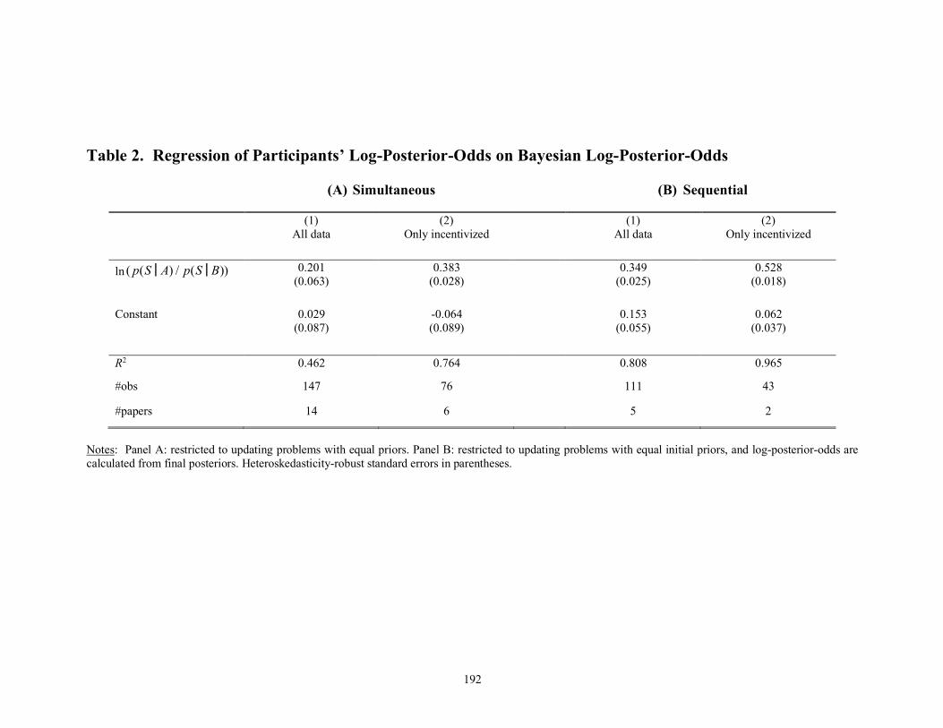
192

Table 2. Regression of Participants’ Log-Posterior-Odds on Bayesian Log-Posterior-Odds

(1) All data

(2) Only incentivized

(1) All data

(2) Only incentivized

ln 0.201 (0.063)

0.383 (0.028)

0.349 (0.025)

0.528 (0.018)

Constant 0.029 (0.087)

-0.064 (0.089)

0.153 (0.055)

0.062 (0.037)

R2 0.462 0.764 0.808 0.965

#obs 147 76 111 43

#papers 14 6 5 2

Notes: Panel A: restricted to updating problems with equal priors. Panel B: restricted to updating problems with equal initial priors, and log-posterior-odds are calculated from final posteriors. Heteroskedasticity-robust standard errors in parentheses.

( p(S Ɉ A) / p(S Ɉ B))

(A) Simultaneous (B) Sequential

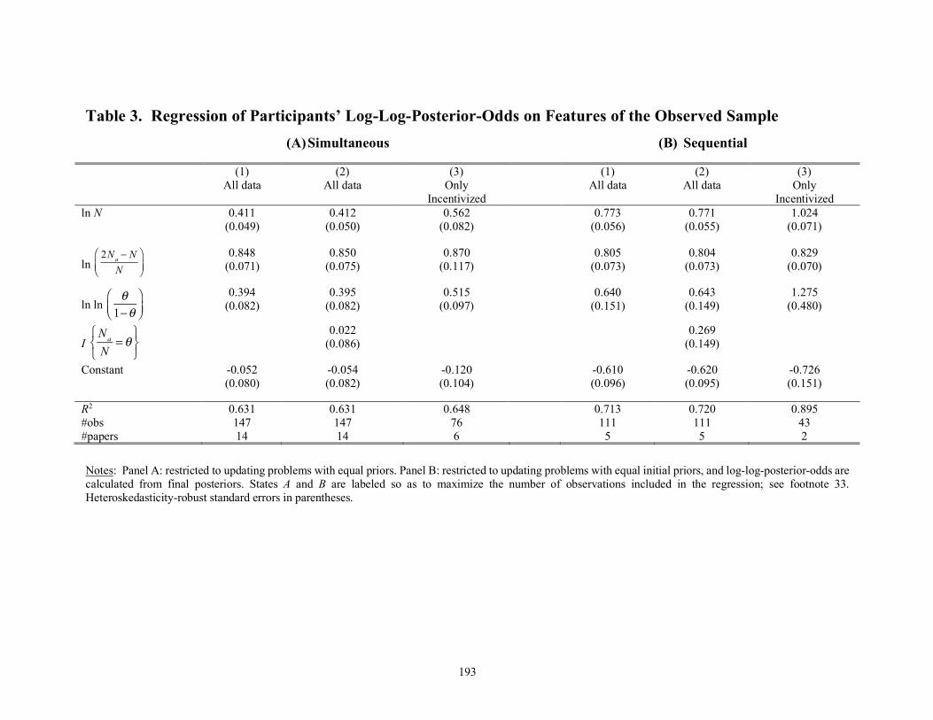
193

Table 3. Regression of Participants’ Log-Log-Posterior-Odds on Features of the Observed Sample

(1) All data

(2) All data

(3) Only

Incentivized

(1) All data

(2) All data

(3) Only

Incentivized ln N 0.411

(0.049) 0.412

(0.050) 0.562

(0.082) 0.773

(0.056) 0.771

(0.055) 1.024

(0.071)

ln 0.848

(0.071) 0.850

(0.075) 0.870

(0.117) 0.805

(0.073) 0.804

(0.073) 0.829

(0.070)

ln ln 0.394

(0.082) 0.395

(0.082) 0.515

(0.097) 0.640

(0.151) 0.643

(0.149) 1.275

(0.480)

I 0.022

(0.086) 0.269

(0.149)

Constant -0.052 (0.080)

-0.054 (0.082)

-0.120 (0.104)

-0.610 (0.096)

-0.620 (0.095)

-0.726 (0.151)

R2 0.631 0.631 0.648 0.713 0.720 0.895 #obs 147 147 76 111 111 43 #papers 14 14 6 5 5 2

Notes: Panel A: restricted to updating problems with equal priors. Panel B: restricted to updating problems with equal initial priors, and log-log-posterior-odds are calculated from final posteriors. States A and B are labeled so as to maximize the number of observations included in the regression; see footnote 33. Heteroskedasticity-robust standard errors in parentheses.

2Na − NN

⎛⎝⎜

⎞⎠⎟

θ1−θ

⎛⎝⎜

⎞⎠⎟

NaN

= θ⎧⎨⎩

⎫⎬⎭

(A) Simultaneous (B) Sequential

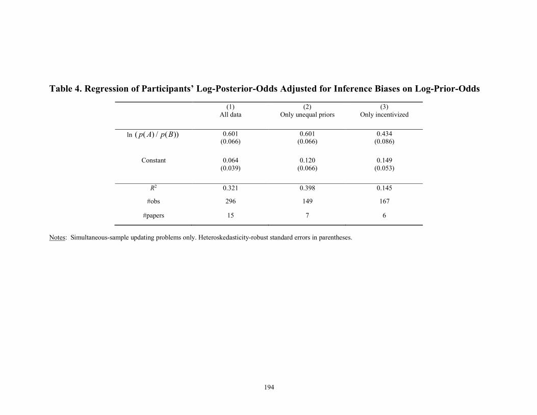
194

Table 4. Regression of Participants’ Log-Posterior-Odds Adjusted for Inference Biases on Log-Prior-Odds

(1) All data

(2) Only unequal priors

(3) Only incentivized

ln 0.601 (0.066)

0.601 (0.066)

0.434 (0.086)

Constant 0.064 (0.039)

0.120 (0.066)

0.149 (0.053)

R2 0.321 0.398 0.145

#obs 296 149 167

#papers 15 7 6

Notes: Simultaneous-sample updating problems only. Heteroskedasticity-robust standard errors in parentheses.

( p(A) / p(B))

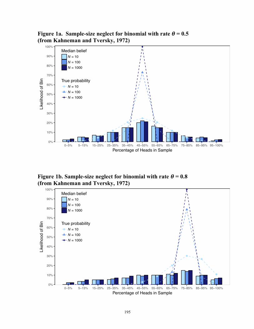
195

Figure 1a. Sample-size neglect for binomial with rate != 0.5 (from Kahneman and Tversky, 1972)

Figure 1b. Sample-size neglect for binomial with rate != 0.8 (from Kahneman and Tversky, 1972)

● ●

●

●

●

●

●

●

●

● ●0%

10%

20%

30%

40%

50%

60%

70%

80%

90%

100%

0−5% 5−15% 15−25% 25−35% 35−45% 45−55% 55−65% 65−75% 75−85% 85−95% 95−100%Percentage of Heads in Sample

Like

lihoo

d of

Bin

Median beliefN = 10N = 100N = 1000

True probability● N = 10

N = 100N = 1000

● ● ● ● ●●

●

●

●

●

●

0%

10%

20%

30%

40%

50%

60%

70%

80%

90%

100%

0−5% 5−15% 15−25% 25−35% 35−45% 45−55% 55−65% 65−75% 75−85% 85−95% 95−100%Percentage of Heads in Sample

Like

lihoo

d of

Bin

Median beliefN = 10N = 100N = 1000

True probability● N = 10

N = 100N = 1000

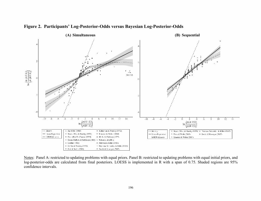
196

Figure 2. Participants’ Log-Posterior-Odds versus Bayesian Log-Posterior-Odds

(A) Simultaneous (B) Sequential

Notes: Panel A: restricted to updating problems with equal priors. Panel B: restricted to updating problems with equal initial priors, and log-posterior-odds are calculated from final posteriors. LOESS is implemented in R with a span of 0.75. Shaded regions are 95% confidence intervals.

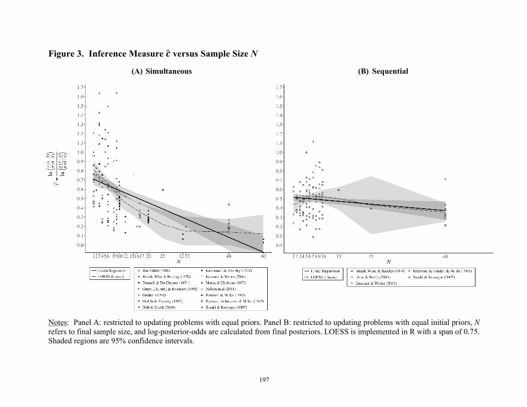
197

Figure 3. Inference Measure !" versus Sample Size N

(A) Simultaneous (B) Sequential

Notes: Panel A: restricted to updating problems with equal priors. Panel B: restricted to updating problems with equal initial priors, N refers to final sample size, and log-posterior-odds are calculated from final posteriors. LOESS is implemented in R with a span of 0.75. Shaded regions are 95% confidence intervals.

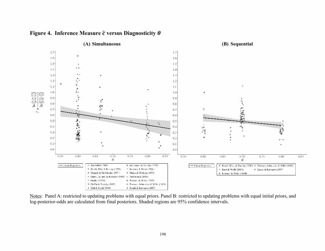
198

Figure 4. Inference Measure !" versus Diagnosticity #

(A) Simultaneous (B) Sequential

Notes: Panel A: restricted to updating problems with equal priors. Panel B: restricted to updating problems with equal initial priors, and log-posterior-odds are calculated from final posteriors. Shaded regions are 95% confidence intervals.

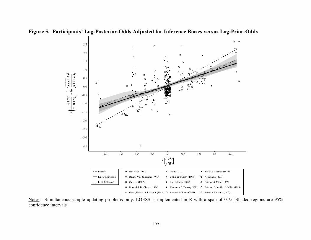
199

Figure 5. Participants’ Log-Posterior-Odds Adjusted for Inference Biases versus Log-Prior-Odds

Notes: Simultaneous-sample updating problems only. LOESS is implemented in R with a span of 0.75. Shaded regions are 95% confidence intervals.