mmn spring0211 lec3-audio.ppt
TRANSCRIPT

Audio Fundamentals, Compression Techniques & Standards
Hamid R. RabieeMostafa Salehi, Fatemeh Dabiran, Hoda Ayatollahi
Spring 2011

Digital Media Lab - Sharif University of Technology2
Outlines
² Audio Fundamentals
² Sampling, digitization, quantization
² μ-law and A-law
² Sound Compression
² PCM, DPCM, ADPCM, CELP, LPC
² Audio Compression
² MPEG Audio Codec
² Perceptual Coding
² MPEG1
² Layer1
² Layer2
² Layer3(MP3)

Sound, sound wave, acoustics
²² SoundSound is a continuous wave that travels through a medium
² Sound waveSound wave: energy causes disturbance in a medium, made of
pressure differences (measure pressure level at a location)
² AcousticsAcoustics is the study of sound: generation, transmission, and
reception of sound waves
² Example is striking a drum
² Head of drum vibrates => disturbs air molecules close to head
² Regions of molecules with pressure above and below equilibrium
² Sound transmitted by molecules bumping into each other
3 Digital Media Lab - Sharif University of Technology

The Characteristics of Sound Waves
² Frequency
² The rate at which sound is measured² Number of cycles per second or Hertz (Hz)² Determines the pitch of the sound as heard by our ears² The higher frequency, the clearer and sharper the sound =>
the higher pitch of sound
² Amplitude
² Sound’s intensity or loudness
² The louder the sound, the larger amplitude.
² All sounds have a duration and successive musical sounds is called rhythm
4 Digital Media Lab - Sharif University of Technology

The Characteristics of Sound Waves (cont.)
distancealong wave
Cycle
Time for one cycleAmplitude
pitch
5
A picture of a sample sound wave
Digital Media Lab - Sharif University of Technology

² To get audio or video into a computer, we must digitize it
² Audio signals are continuous in time and amplitude
² Audio signal must be digitized in both time and amplitude
to be represented in binary form.
6
Audio Digitization
Analog-Digital Converter (ADC)
Voice 10010010000100
Sinusoid wave
Digital Media Lab - Sharif University of Technology

Human Perception
² Speech is a complex waveform
² Vowels (a,i,u,e,o) and bass sounds are low frequencies
² Consonants (s,sh,k,t,…) are high frequencies
² Humans most sensitive to low frequencies
²Most important region is 2 kHz to 4 kHz
² Hearing dependent on room and environment
² Sounds masked by overlapping sounds
² Temporal & Frequency masking
7 Digital Media Lab - Sharif University of Technology

Audio Digitization (cont.)
² Step1. Sampling -- divide the horizontal axis (the time
dimension) into discrete pieces. Uniform sampling is
ubiquitous (everywhere at once).
8 Digital Media Lab - Sharif University of Technology

Nyquist Theorem
² Suppose we are sampling a waveform. How often do we
need to sample it to figure out its frequency?
• The NyquistNyquist TheoremTheorem, also known as the sampling theorem, is a principle that engineers follow in the digitization of analog signals.
• For analog-to-digital conversion (ADC) to result in a faithful reproduction of the signal, slices, called samples, of the analog waveform must be taken frequently.
•The number of samples per second is called the sampling rate orsampling frequency.
9 Digital Media Lab - Sharif University of Technology

Nyquist Theorem (cont.)
² Nyquist rate -- It can be proven that a bandwidth-limited
signal can be fully reconstructed from its samples, if the
sampling rate is at least twice the highest frequency in the
signal.
² The highest frequency component, in hertz, for a given
analog signal is fmax.
² According to the Nyquist Theorem, the sampling rate must
be at least 2fmax, or twice the highest analog frequency
component
10 Digital Media Lab - Sharif University of Technology

11
² Step2. Quantization -- Converts actual amplitude sample values (usually voltage measurements) into an integer approximation
² Tradeoff between number of bits required and error² Human perception limitations affect allowable error
² Specific application affects allowable error
² Once samples have been captured (Discrete in time by sampling –Nyquist), they must be made discrete in amplitude (Discrete in amplitude by quantization).
² Two approaches to quantization² Rounding the sample to the closest integer. ² (e.g. round 3.14 to 3)
² Create a Quantizer table that generates a staircase pattern of values based on a step size.
Quantization
Digital Media Lab - Sharif University of Technology

12
Reconstruction
² Analog-to-Digital Converter (ADC) provides the sampled and
quantized binary code.
² Digital-to-Analog Converter (DAC) converts the quantized
binary code back into an approximation of the analog signal
(reverses the quantization process) by clocking the code to the
same sample rate as the ADC conversion.
Digital Media Lab - Sharif University of Technology

13
Quantization Error
² After quantization, some information is lost
² Errors (noise) introduced
² The difference between the original sample value and the
rounded value is called the quantization error
² A Signal to Noise Ratio (SNR) is the ratio of the relative sizes of the
signal values and the errors.
² The higher the SNR, the smaller the average error is with
respect to the signal value, and the better the fidelity.
Quantization is only an approximation.
Digital Media Lab - Sharif University of Technology

μ-law, A-law
² Non-uniform quantizers: Difficult to make, Expensive.
² Solution: Companding => Uniform Q. => Expanding
14 Digital Media Lab - Sharif University of Technology

μ--law, Alaw, A--law (cont.)law (cont.)
15
North America andJapan
Europe
Digital Media Lab - Sharif University of Technology

μ-law vs. A-law
² 8-bit μ-law used in US for telephony
² ITU Recommendation G.711
² 8-bit A-law used in Europe for telephony
² Similar, but a slightly different curve.
² Both give similar quality to 12-bit linear encoding.
² A-law used for International circuits.
² Both are linear approximations to a log curve.
² 8000 samples/sec * 8bits per sample = 64Kb/s data rate
Digital Media Lab - Sharif University of Technology16
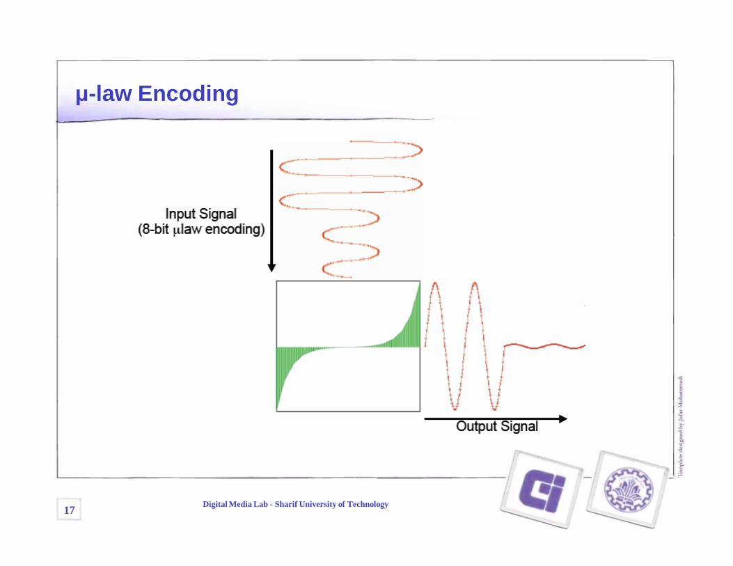
μ-law Encoding
Digital Media Lab - Sharif University of Technology17

μ-law Decoding
Digital Media Lab - Sharif University of Technology18

AUDIO & SOUND COMPRESSION TECHNIQUES
19 Digital Media Lab - Sharif University of Technology

Sound Compression
² Some techniques for sound compression:² PCM - send every sample
² DPCM - send differences between samples
² ADPCM - send differences, but adapt how we code them
² LPC - linear model of speech formation
² CELP - use LPC as base, but also use some bits to code corrections for the things
LPC gets wrong.
² The techniques that code received sound signals² PCM, DPCM, ADPCM
² The techniques that parameterize the sound model (model-based
coding)² LPC, CELP
20 Digital Media Lab - Sharif University of Technology

Pulse-code Modulation (PCM)
² μ-law and a-law PCM have already reduced the data sent.
² However, each sample is still independently encoded.² In reality, samples are correlated.
² Can utilize this correlation to reduce the data sent.
Digital Media Lab - Sharif University of Technology21

Pulse-code Modulation (PCM)
² Digital Representation of an Analog Signal
² Sampling and Quantization
² Parameters:
² Sampling Rate (Samples per Second)
² Quantization Levels (Bits per Sample)
Digital Media Lab - Sharif University of Technology22

Adaptive DPCM (ADPCM)
² Makes a simple prediction of the next sample, based on weighted previous
n samples.
² Normally the difference between samples is relatively small and can be
coded with less than 8 bits.
² Typically use 6 bits for difference, rather than 8 bits for absolute value.
² Compression is lossy, as not all differences can be coded
Digital Media Lab - Sharif University of Technology23

Differential PCM (DPCM)
² Different Coding techniques in comparison with DPCM
² 2 Methods
² Adaptive Quantization
² Quantization levels are adaptive, based on the content of the audio.
² Adaptive Prediction
² Receiver runs same prediction algorithm and adaptive quantization levels
to reconstruct speech.
Digital Media Lab - Sharif University of Technology24

Model-based Coding
² PCM, DPCM and ADPCM directly code the received audio signal.
² An alternative approach is to build a parameterized model of the
² sound source (i.e.. Human voice).
² For each time slice (e.g. 20ms):
² Analyze the audio signal to determine how the signal was produced.
² Determine the model parameters that fit.
² Send the model parameters.
² At the receiver, synthesize the voice from the model and received
parameters.
Digital Media Lab - Sharif University of Technology25

Speech formation
² Voiced sounds: series of pulses of air as larynx opens and closes. Basic
tone then shaped by changing resonance of vocal tract.
² Unvoiced sounds: larynx held open, turbulent noise made in mouth.
Digital Media Lab - Sharif University of Technology26
LPC
² Introduced in 1960s.
² Low-bitrate encoder:
² 1.2Kb/s - 4Kb/s
² Sounds very synthetic
² Basic LPC mostly used where bitrate really matters (eg in miltary
applications)
² Most modern voice codecs (eg GSM) are based on enhanced LPC
encoders.
Digital Media Lab - Sharif University of Technology27

LPC
² Digitize signal, and split into segments (eg 20ms)
² For each segment, determine:
² Pitch of the signal (i.e. basic formant frequency)
² Loudness of the signal.
² Whether sound is voiced or unvoiced
² Voiced: vowels, “m”, “v”, “l”
² Unvoiced: “f”, “s”
² Vocal tract excitation parameters (LPC coefficients)
Digital Media Lab - Sharif University of Technology28
Limitations of LPC Model
² LPC linear predictor is very simple.
² For this to work, the vocal tract “tube” must not have any side branches
(these would require a more complex model).
² OK for vowels (tube is a reasonable model)
² For nasal sounds, nose cavity forms a side branch.
² In practice this is ignored in pure LPC.
² More complex codecs attempt to code the residue signal, which helps correct
this.
Digital Media Lab - Sharif University of Technology29

Code Excited Linear Prediction (CELP)
² Goal is to efficiently encode the residue signal, improving speech quality
over LPC, but without increasing the bit rate too much.
² CELP codecs use a codebook of typical residue values.
² Analyzer compares residue to codebook values.
² Chooses value which is closest.
² Sends that value.
² Receiver looks up the code in its codebook, retrieves the residue, and uses
this to excite the LPC formant filter.
Digital Media Lab - Sharif University of Technology30

CELP
² Problem is that codebook would require different residue values for every
possible voice pitch.
² Codebook search would be slow, and code would require a lot of bits to send.
² One solution is to have two codebooks.
² One fixed by codec designers, just large enough to represent one pitch period of
residue.
² One dynamically filled in with copies of the previous residue delayed by various
amounts (delay provides the pitch)
² CELP algorithm using these techniques can provide pretty good quality at
4.8Kb/s.
Digital Media Lab - Sharif University of Technology31

Enhanced LPC Usage
² GSM (Groupe Speciale Mobile)² Residual Pulse Excited LPC
² 13Kb/s
² LD-CELP² Low-delay Code-Excited Linear Prediction (G.728)
² 16Kb/s
² CS-ACELP² Conjugate Structure Algebraic CELP (G.729)
² 8Kb/s
² MP-MLQ² Multi-Pulse Maximum Likelihood Quantization (G.723.1)
² 6.3Kb/s
Digital Media Lab - Sharif University of Technology32

Audio Compression
² LPC-based codecs model the sound source to achieve good compression.
² Works well for voice.
² Terrible for music.
² What if you can’t model the source?
² Model the limitations of the human ear.
² Not all sounds in the sampled audio can actually be heard.
² Analyze the audio and send only the sounds that can be heard.
² Quantize more coarsely where noise will be less audible.
² Audio vs. Speech
² Higher quality requirement for audio
² Wider frequency range of audio Sound Signal
Digital Media Lab - Sharif University of Technology33

34
Psychoacoustics Model
² Dynamic range is ratio of maximum signal amplitude to minimum signal
amplitude (measured in decibels).
² D = 20 log (Amax/Amin) dB
² Human hearing has dynamic range of ~ 96dB
² Sensitivity of the ear is dependent on frequency.
² Most sensitive in range of 2-5KHz
Digital Media Lab - Sharif University of Technology
Sensitivity of human ears

Psychoacoustics Model
² Amplitude Sensitivity
² Frequencies only heard if they exceed a sensitivity threshold:
Digital Media Lab - Sharif University of Technology35

36
Psychoacoustics Model
² Frequency Masking
² The sensitivity threshold curve is distorted by the presence of loud sounds.
² Frequencies just above and below the frequency of a loud sound need to be
louder than the normal minimum amplitude before they can be heard.
² Thinking: if there is a 8 kHz signal at 60 dB, can we hear another 9 kHz signal
at 40 dB?
Digital Media Lab - Sharif University of Technology

Masking Curves for Loud Sounds
Digital Media Lab - Sharif University of Technology37

38
Psychoacoustics Model
² Temporal masking² If we hear a loud sound, then it stops, it takes a little while until we
can hear a soft tone nearby
² After hearing a loud sound, the ear is deaf to quieter sounds in the same
frequency range for a short time.
Digital Media Lab - Sharif University of Technology

Principle of Audio Compression
² Audio compression – Perceptual coding
² Take advantage of psychoacoustics model
² Distinguish between the signal of different sensitivity to human ears
² Signal of high sensitivity – more bits allocated for coding
² Signal of low sensitivity – less bits allocated for coding
² Exploit the frequency masking
² Don’t encode the masked signal (range of masking is 1 critical band)
² Exploit the temporal masking
² Don’t encode the masked signal
39 Digital Media Lab - Sharif University of Technology

AUDIO CODING STANDARDS
40 Digital Media Lab - Sharif University of Technology

Audio Coding Standards
² G.711 - A-LAW/U-LAW encodings (8 bits/sample)
² G.721 - ADPCM (32 kbs, 4 bits/sample)
² G.723 - ADPCM (24 kbs and 40 kbs, 8 bits/sample)
² G.728 - CELP (16 kbs)
² LPC (FIPS-1015) - Linear Predictive Coding (2.4kbs)
² CELP (FIPS-1016) - Code excited LPC (4.8kbs, 4bits/sample)
² G.729 - CS-ACELP (8kbs)
² MPEG1/MPEG2, AC3 - (16-384kbs) mono, stereo, and 5+1 channels
You can find a complete table of coding standards on course web page!You can find a complete table of coding standards on course web page!
Digital Media Lab - Sharif University of Technology41

MPEG Audio Codec
² MPEG (Motion Picture Expert Group) and ISO (International Standard
Organization) have published several standards about digital audio
coding.
² MPEG-1 Layer 1,2 and 3 (MP3)
² MPEG2 AAC
² MPEG4 AAC and TwinVQ
² They have been widely used in consumer electronics, digital audio
broadcasting, DVD and movies etc.
42 Digital Media Lab - Sharif University of Technology

43
MPEG Audio Codec
² Procedure of MPEG audio coding
² Apply DFT (Discrete Fourier Transform) decomposes the audio into frequency
subbands that approximate the 32 critical bands (sub-band filtering)
² Use psychoacoustics model in bit allocation
² If the amplitude of signal in band is below the masking threshold, don’t encode
² Otherwise, allocate bits based on the sensitivity of the signal
² Multiplex the output of the 32 bands into one bitstream
Digital Media Lab - Sharif University of Technology

MPEG1 Audio Layer 1
² MPEG 1 audio allows sampling rate at 44.1 48, 32, 22.05, 24 and 16KHz.
² MPEG1 filters the input audio into 32 bands.
FilteringAnd
downsampling
Audio
samples
12 samples12 samples
12 samples
Perceptualcoder
NormalizeBy scalefactor
44 Digital Media Lab - Sharif University of Technology

MPEG1 Audio Layer 2
² Layer 2 is very similar to Layer 1, but groups 3 12-samples together in
coding.
² It also improves the scaling factor quantization and also groups 3 audio
samples together in bit assignment.
FilteringAnd
downsampling
Audiosamples
36 samples36 samples
36samples
Perceptualcoder
NormalizeBy scalefactor
45 Digital Media Lab - Sharif University of Technology

MPEG Audio Layer 3 : MP3
² MP3 is another layer built on top of MPEG1 audio layer 2.
² MP3 then uses Huffman coding to further compress the bit streams
losslessly.
46 Digital Media Lab - Sharif University of Technology

MPEG Audio
Digital Media Lab - Sharif University of Technology47

Next Session
Image
48Digital Media Lab - Sharif University of Technology