midterm exam (post-test revision version) problem 1...

Victor Ying Math 470

Spring 2011 Midterm Exam (post-test revision version)

of 21

Problem 1. Carefully read example 7.9 at page 179 regarding Gibbs Sampler. Then answer

problem 7.20 at page 193.

(a) Modify this program to sample from bivariate normal distribution with zero means, unit standard

deviations, and . Report your results. If you worked Problem 7.18, compare with those

results.

The results are similar to those from the original code used in example 7.9, except that the - and -

values are less correlated as illustrated in the plots below.

Plot:



of 21

Codes: set.seed(1235); m = 20000; rho.vec = c(.8, .6); label.vec = c("rho = 0.8", "rho =

0.6")

par(mfrow = c(2,2), pty="s")

for( j in 1:2)

{

sgm = sqrt(1 - rho.vec[j]^2)

xc = yc = numeric(m) # vectors of state components

xc[1] = -3; yc[1] = 3 # arbitrary starting values

for (i in 2:m)

{

xc[i] = rnorm(1, rho.vec[j]*yc[i-1], sgm)

yc[i] = rnorm(1, rho.vec[j]*xc[i], sgm)

}

x = xc[(m/2+1):m]; y = yc[(m/2+1):m] # states after burn-in

round(c(mean(x), mean(y), sd(x), sd(y), cor(x,y)), 4)

best = pmax(x,y); mean(best >= 1.25) # prop. getting certif.

summary(best)

hist(best, prob=T, col="wheat", main=label.vec[j])

abline(v = 1.25, lwd=2, col="red")

plot(x, y, xlim=c(-4,4), ylim=c(-4,4), pch=".", main=label.vec[j])

lines(c(-5, 1.25, 1.25), c(1.25, 1.25, -5), lwd=2, col="red")

}

par(mfrow = c(1,1), pty="m")

(b) Run the original program (with ) and make an autocorrelation plot of -values from /2

on, as in part (c) of Problem 7.19. If you worked that problem, compare the two autocorrelation

functions.

The autocorrelation function from part (c) of Problem 7.19 decreases much faster. Both appear to

oscillate up and down somewhat as lag increases. Here is the autocorrelation plot (when )



of 21

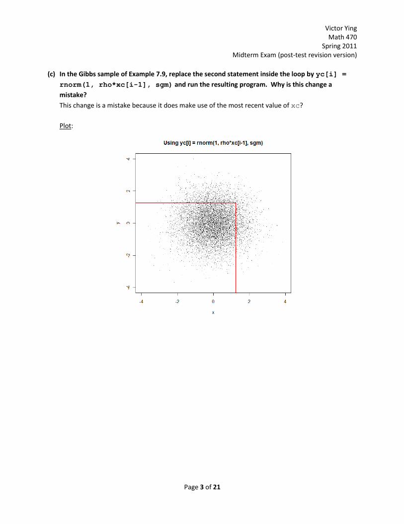
(c) In the Gibbs sample of Example 7.9, replace the second statement inside the loop by yc[i] =

rnorm(1, rho*xc[i-1], sgm) and run the resulting program. Why is this change a

mistake?

This change is a mistake because it does make use of the most recent value of xc?

Plot:



of 21

Problem 2 (Problem 3.27 at page 83 in the text). Modify the program of Example 3.9 to

approximate the volume beneath the bivariate standard normal density surface and above two

additional regions of integration as specified below. Use both the Riemann and Monte Carlo methods

in parts (a) and (b), with .

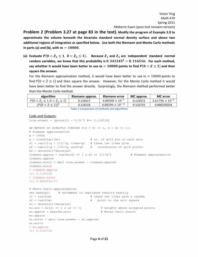
(a) Evaluate * +. Because and are independent standard normal

random variables, we know that this probability is . For each method,

say whether it would have been better to use points to find * + and then

square the answer.

For the Riemann approximation method, it would have been better to use points to

find * + and then square the answer. However, for the Monte Carlo method it would

have been better to find the answer directly. Surprisingly, the Riemann method performed better

than the Monte Carlo method.

algorithm Riemann approx. Riemann error MC approx. MC error * + 0.116517 0.116572

( * +) 0.116516 0.116755 0.000239254 Table 1 Comparison of methods and algorithms

Code and Outputs: true.answer = (pnorm(1) - 0.5)^2 #== 0.1165162

## METHOD OF DIRECTLY FINDING P{0 < Z1 <= 1, 0 < Z2 <= 1}:

# Riemann approximation

m = 10000

g = round(sqrt(m)) # no. of grid pts on each axis

x1 = rep((1:g - 1/2)/g, times=g) # these two lines give

x2 = rep((1:g - 1/2)/g, each=g) # coordinates of grid points

hx = dnorm(x1)*dnorm(x2)

riemann.approx = sum(hx[x1 <= 1 & x2 <= 1])/g^2 # Riemann approximation

riemann.approx

riemann.error = abs( true.answer - riemann.approx)

riemann.error

> riemann.approx

[1] 0.1165169

> riemann.error

[1] 6.883003e-07

# Monte Carlo approximation

set.seed(pi) # uncomment to reproduce results exactly

u1 = runif(m) # these two lines give a random

u2 = runif(m) # point in the unit square

hu = dnorm(u1)*dnorm(u2)

hu.acc = hu[u1 <= 1 & u2 <= 1] # heights above accepted points

mc.approx = mean(hu.acc) # Monte Carlo result

mc.approx

mc.error = abs( true.answer - mc.approx)

mc.error

> mc.approx

[1] 0.1165724



of 21

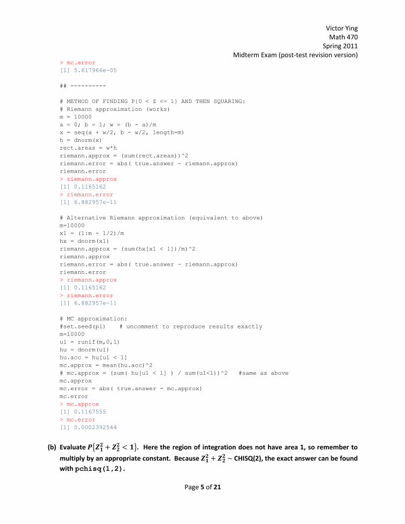
> mc.error

[1] 5.617966e-05

## ----------

# METHOD OF FINDING P{0 < Z <= 1} AND THEN SQUARING:

# Riemann approximation (works)

m = 10000

a = 0; b = 1; w = (b - a)/m

x = seq(a + w/2, b - w/2, length=m)

h = dnorm(x)

rect.areas = w*h

riemann.approx = (sum(rect.areas))^2


riemann.error

> riemann.approx

[1] 0.1165162

> riemann.error

[1] 6.882957e-11

# Alternative Riemann approximation (equivalent to above)

m=10000

x1 = (1:m - 1/2)/m

hx = dnorm(x1)

riemann.approx = (sum(hx[x1 < 1])/m)^2

riemann.approx


riemann.error

> riemann.approx

[1] 0.1165162

> riemann.error

[1] 6.882957e-11

# MC approximation:

#set.seed(pi) # uncomment to reproduce results exactly

m=10000

u1 = runif(m,0,1)

hu = dnorm(u1)

hu.acc = hu[u1 < 1]

mc.approx = mean(hu.acc)^2

# mc.approx = (sum( hu[u1 < 1] ) / sum(u1<1))^2 #same as above

mc.approx

mc.error = abs( true.answer - mc.approx)

mc.error

> mc.approx

[1] 0.1167555

> mc.error

[1] 0.0002392544

(b) Evaluate {

}. Here the region of integration does not have area 1, so remember to

multiply by an appropriate constant. Because

CHISQ(2), the exact answer can be found

with pchisq(1,2).



of 21

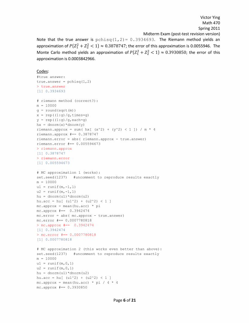
Note that the true answer is pchisq(1,2)= 0.3934693. The Riemann method yields an

approximation of *

+ ; the error of this approximation is 0.0055946. The

Monte Carlo method yields an approximation of *

+ ; the error of this

approximation is 0.0003842966.

Codes: #true answer:

true.answer = pchisq(1,2)

> true.answer

[1] 0.3934693

# riemann method (correct?):

m = 10000

g = round(sqrt(m))

x = rep((1:g)/g,times=g)

y = rep((1:g)/g,each=g)

hx = dnorm(x)*dnorm(y)

riemann.approx = sum( hx[ (x^2) + (y^2) < 1 ]) / m * 4

riemann.approx #== 0.3878747

riemann.error = abs( riemann.approx - true.answer)

riemann.error #== 0.005594673

> riemann.approx

[1] 0.3878747

> riemann.error

[1] 0.005594673

# MC approximation 1 (works):

set.seed(1237) #uncomment to reproduce results exactly

m = 10000

u1 = runif(m,-1,1)

u2 = runif(m,-1,1)


hu.acc = hu[ (u1^2) + (u2^2) < 1 ]

mc.approx = mean(hu.acc) * pi

mc.approx #== 0.3942474

mc.error = abs( mc.approx - true.answer)

mc.error #== 0.0007780818

> mc.approx #== 0.3942474

[1] 0.3942474

> mc.error #== 0.0007780818

[1] 0.0007780818

# MC approximation 2 (this works even better than above):

set.seed(1237) #uncomment to reproduce results exactly

m = 10000

u1 = runif(m,0,1)

u2 = runif(m,0,1)


hu.acc = hu[ (u1^2) + (u2^2) < 1 ]

mc.approx = mean(hu.acc) * pi / 4 * 4

mc.approx #== 0.3930850



of 21

mc.error = abs( mc.approx - true.answer)

mc.error #== 0.0003842966

> mc.approx #== 0.3930850

[1] 0.3930850

> mc.error #== 0.0003842966

[1] 0.0003842966

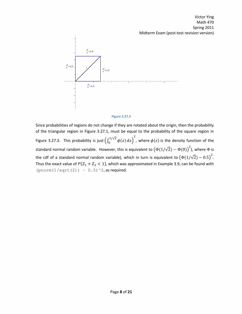
(c) The joint density function of ( ) has circular contour lines centered at the origin, so that

probabilities of regions do not change if they are rotated about the origin. Use this fact to argue

that the exact value of * +, which was approximated in Example 3.9, can be found

with (pnorm(1/sqrt(2)) – 0.5)^2.

Consider the series of rotations about the origin illustrated in Figures 3.27.1 through 3.27.3. This

response will continue after the break.

Figure 3.27.1

Figure 3.27.2

0.5 1 1.5 2 2.5

1.2

1

0.8

0.6

0.4

0.2

-0.2

-0.4

-0.6

1

1

2

0.5 1 1.5 2 2.5

1.2

1

0.8

0.6

0.4

0.2

-0.2

-0.4

-0.6

1

1

2



of 21

Figure 3.27.3

Since probabilities of regions do not change if they are rotated about the origin, then the probability

of the triangular region in Figure 3.27.1, must be equal to the probability of the square region in

Figure 3.27.3. This probability is just (∫ ( ) √

)

, where ( ) is the density function of the

standard normal random variable. However, this is equivalent to ( ( √ ) ( ))

(, where is

the cdf of a standard normal random variable), which in turn is equivalent to ( ( √ ) )

.

Thus the exact value of * +, which was approximated in Example 3.9, can be found with

(pnorm(1/sqrt(2)) – 0.5)^2, as required.

0.5 1 1.5 2 2.5

1.2

1

0.8

0.6

0.4

0.2

-0.2

-0.4

-0.6

1

2

2= 1/ 2

2

2= 1/ 2

2

2= 1/ 2

2

2= 1/ 2



of 21

Problem 3. Buffon’s needle problem asks…

(a) Show the probability that the needle crosses a line is

.

Wikipedia said:

The uniform probability density function of between 0 and is

. The uniform probability

density function of between 0 and

is

. Since x and \theta are independent then their joint

probability density function is the product

The needle crosses the line if

Final the probability of the needle crossing a line is

∫ ∫

( )

(b) Describe how you could use this result to obtain a Monte Carlo estimate of the value .

From part (a), we know that the probability the needle crosses the line is

( )

However, we can simulate the dropping of the needle a lot of times to estimate the probability the

needle crosses the line with the proportion of trials where the needle crossed the line. Let be the

simulated proportion. Then we have

Rearranging terms from the equation above, we have

So, to get a Monte Carlo estimate of , run a large number of simulation to get . Then plug in the

values of into the above equation to get your estimate.

(c) Write a computer program that simulates needled dropping and use it to estimate .

Our Monte Carlo approximation for is 3.138279.

Code and Output: #set.seed(1234)

l = 1

t = 2

m = 1000000

x = runif(m,0,t/2)

theta = runif(m,0,pi/2)

indicator = logical(m)



of 21

for( i in 1:m)

{

if ( (l/2) * cos( theta[i]) > x[i] ) indicator[i] = TRUE

}

p = mean(indicator) #theoretical answer (2*l)/(t*pi)

#estimation of pi:

(2*l)/(t*p)

> (2*l)/(t*p)

[1] 3.138279



of 21

Problem 4 (Problem 7.19. MCMC: Metropolis and Metroplis-Hastings algorithms

at page 191 in the text.). Consider the following modifications of the program of Example 7.8.

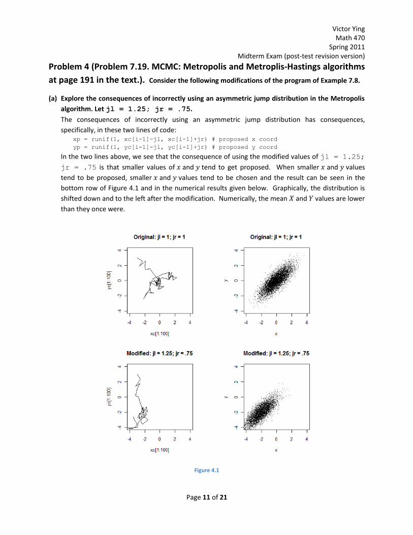
(a) Explore the consequences of incorrectly using an asymmetric jump distribution in the Metropolis

algorithm. Let jl = 1.25; jr = .75.

The consequences of incorrectly using an asymmetric jump distribution has consequences,

specifically, in these two lines of code: xp = runif(1, xc[i-1]-jl, xc[i-1]+jr) # proposed x coord

yp = runif(1, yc[i-1]-jl, yc[i-1]+jr) # proposed y coord

In the two lines above, we see that the consequence of using the modified values of jl = 1.25;

jr = .75 is that smaller values of and tend to get proposed. When smaller and values

tend to be proposed, smaller and values tend to be chosen and the result can be seen in the

bottom row of Figure 4.1 and in the numerical results given below. Graphically, the distribution is

shifted down and to the left after the modification. Numerically, the mean and values are lower

than they once were.

Figure 4.1



of 21

Original Results: > round(c(mean(x), mean(y), sd(x), sd(y), cor(x,y)), 4)

[1] -0.0348 -0.0354 0.9966 0.9992 0.7994

> mean(diff(x)==0) # proportion or proposals rejected

[1] 0.4316216

> mean(pmax(x,y) >= 1.25) # prop. of subj. getting certificates

[1] 0.14725

Results After Modification: > round(c(mean(x), mean(y), sd(x), sd(y), cor(x,y)), 4)

[1] -2.1755 -2.1742 1.0046 0.9986 0.8158

> mean(diff(x)==0) # proportion or proposals rejected

[1] 0.5826291

> mean(pmax(x,y) >= 1.25) # prop. of subj. getting certificates

[1] 9e-04

(b) The Metropolis-Hastings algorithm permits and adjusts for use of an asymmetric jump distribution

by modifying the acceptance criterion. Specifically, the ratio of variances is multiplied by a factor

that corrects for the bias due to the asymmetric jump function. In our example, this

“symmetrization" amounts to restricting jumps in and to 0.75 units in either direction. The

program below [(removed in the interest of saving paper)] modifies the one in Example 7.8 to

implement the Metropolis-Hastings algorithm; the crucial change is the use of the adjustment

factor adj inside the loop. Interpret the numerical results, the scatterplot (as in Figure 7.17,

upper right), and the histogram.

Interpretation:

The numerical results, scatterplot, and histogram are given below (after the interpretation). The use

of the adjustment factor has successfully corrected for the bias due to the asymmetric jump

function. As can be seen from the numerical results below, the means, standard deviations, and

correlation of and have returned to values that are much closer to their original values

(compare the results below to the data above in the “Original Restults” section of part (a)). The

scatterplot in Figure 4.2 further supports the conclusion that the use of the adjustment factor has

corrected the “southwesterly” bias that was evident in the bottom-right plot of Figure 4.1 above.

Finally, in Figure 4.3 we have histogramed of the lengths of the jumps in the x-direction; it is

somewhat symmetric about 0, indicating that longer negative jumps responsible for asymmetry are

being rejected (Suess & Trumbo 192)?

Results, Scatterplot, and Histogram: > round(c(mean(x), mean(y), sd(x), sd(y), cor(x,y)) ,4)

[1] 0.0017 0.0058 1.0270 1.0330 0.8139

> mean(diff(xc)==0); mean(pmax(x, y) > 1.25)

[1] 0.6290963

[1] 0.1547



of 21

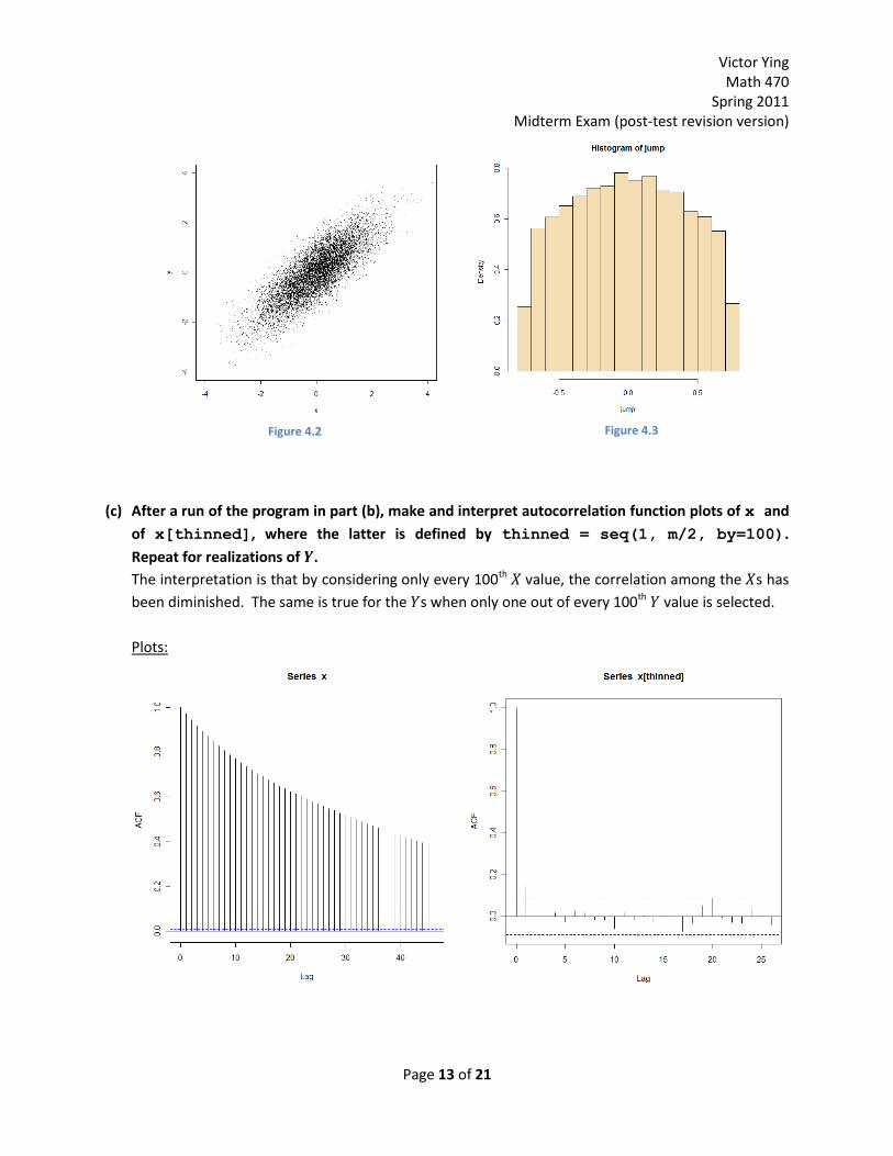
Figure 4.2

Figure 4.3

(c) After a run of the program in part (b), make and interpret autocorrelation function plots of x and

of x[thinned], where the latter is defined by thinned = seq(1, m/2, by=100).

Repeat for realizations of .

The interpretation is that by considering only every 100th value, the correlation among the s has

been diminished. The same is true for the s when only one out of every 100th value is selected.

Plots:



of 21



of 21

Problem 5. Carefully read example 5.4 at page 130. Then answer problem 5.19 at page 138. (A

general form of Bayes’ Theorem.)

(a) Using with appropriate subscripts to denote joint, marginal, and conditional density functions,

we can state a form of Bayes’ Theorem that applies to distributions generally, not just to

probabilities of events,

( ) ( )

( )

( )

∫ ( )

( ) ( )

∫ ( ) ( )

where the integrals are taken over the real line. Give reasons for each step in this equation.

(Compare this results with equation (5.7).)

The first equality come from the fact that

( ) ( ) ( ) (5.1) The second comes from the fact that a marginal distribution can be derived by integrating the joint

distribution over the other variable(s). The third equality also comes from (5.1).

(b) In Example 5.3, ( ) is the potency of a randomly chosen batch of drug, and it is

assayed as * + ( ). The expression for the posterior density in part (a) allows us

to find the probability that a batch is good given that it assayed at 100.5, thus barely failing

inspection. Explain why this is not the same as .

Let

( )

as in equation (5.6) from the book. Then, in our case, is the probability that a batch has a potency

of 101 or less given that it is assayed at 101 or less, and is the probability that a batch has a

potency greater than 101 given that it is assayed at 101 or less.

is different from the probability that a batch is good given that it assayed at 101 or less

because each of these two probabilities deals with a different event; the event that a batch is both

good and is assayed at 101 or less is the same as the event that a batch both has potency greater

than 100 and is assayed at 101 or less. On the other hand, deals with the event that a batch

has potency greater than 101 given that it is assayed at 101 or less?

(c) We seek * +. Recalling the distribution of from Example 5.3 and using the

notation of Problem 5.14, show that this probability can be evaluated as follows:

∫ ( )

∫ ( ) ( )

( )

We have

∫ ( )

∫ ( ) ( )

( )

( )

∫ ( ) ( )

( )



of 21

∫ ( ) ( )

( )

(5.2)

where the second equality comes from the fact (on page 128 of the text) that we have

( ), ( ), and ( √

).

(d) The R code below implements Riemann approximation of the probability in part (c). Run the

program and provide a numerical answer (roughly 0.8) to three decimal places. In Chapter 8, we

will see how to find the exact conditional distribution * +, which is normal. For now,

carefully explain why this R code can be used to find the required probability. s = seq(100, 130, 0.001)

numer = 30 * mean(dnorm(s, 110, 5) * dnorm(100.5, s, 1))

denom = dnorm(100.5, 110, 5.099)

numer/denom

The reason that the points of evaluation in s (whose largest value is 130) works despite the fact that

the upper limit of integration is infinity is that the standard deviations of the normal density

functions in the numerator are so small. Specifically, for ( ), 130 is four

standard deviations from the mean 110. For ( ), 100.5 is 29.5 standard

deviation from the largest mean—130—under consideration. The probabilities at such distances

from the mean in a normal distribution are negligibly small.

Code and Output: > s = seq(100, 130, 0.001)

> numer = 30 * mean(dnorm(s, 110, 5) * dnorm(100.5, s, 1))

> denom = dnorm(100.5, 110, 5.099)

> numer/denom

[1] 0.8113713



of 21

Problem 6. (Problem 6.5 at page 155 (2-state Markov chains))

Several processes are described below. For each of them evaluate (i) * +, (ii)

* +, (iii) * +, and (iv) * +. Also,

(v) say whether the process is a 2-state homogeneous Markov chain. If not, show how it fails to

satisfy the Markov property. If so, give its 1-stage transition matrix .

(a) Each is determined by an independent toss of a coin, taking the value 0 if the coin shows Tails

and 1 if it shows Heads, with ( ) .

We have the following:

(i) * + * +

(ii) * + * +

(iii) * + * +

(iv) * + * +

(v) This is a 2-state homogeneous Markov chain. Its 1-stage transition matrix is

*

+

Note that the first equations in (i) through (iv) follow from independence of the s.

(b) The value of is determined by whether a toss of a fair coin is Tails (0) or Heads (1), and is

determined similarly by a second independent toss of the coin. For , for odd ,

and for even .

(i) * + * +

* +

(ii) * + * +

(iii) * + * +

(iv) * + * +

(v) This is a 2-state homogeneous Markov chain with 1-stage transition matrix

{*

+

*

+

(c) The value of is 0 or 1, according to whether the roll of a fair die gives a Six (1) or some other

value (0). For each step , if a roll of the die shows Six on the th roll, then ;

otherwise, .

(i) * + * +



of 21

(ii) * + * + * +

(iii) * + * + * +

(iv) * +

* + * + * +

* +

(

)

(

)

(v) This is a two-state homogeneous Markov chain with 1-step transition matrix

[

]

(d) Start with . For , a fair die is rolled. If the maximum value shown on the die at any

of the steps is smaller than 6, then ; otherwise .

(i) * + .

(ii) * + .

(iii) * +

(iv) * + ( )( )

(v) This is a two-state homogeneous Markov chain with 1-step transition matrix

*

+

(e) At each step , a fair coin is tossed and takes the value if the coin shows Tails and 1 if

it shows Heads. Starting with , the value of for is determined by

( )

The process is sometimes called a “random walk” on the points 0, 1, 2, and 3, arranged around

a circle (with 0 adjacent to 3). Finally, , if ; otherwise

(i) * + .



of 21

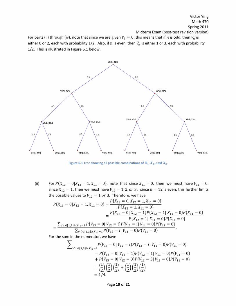
For parts (ii) through (iv), note that since we are given , this means that if is odd, then is

either 0 or 2, each with probability 1/2. Also, if is even, then is either 1 or 3, each with probability

1/2. This is illustrated in Figure 6.1 below.

Figure 6.1 Tree showing all possible combinations of

(ii) For * +, note that since , then we must have .

Since , then we must have ; since is even, this further limits

the possible values to Therefore, we have

* + * +

* +

* + * + * +

* + * +

∑ * + * + * + * +

∑ * + * + * +

For the sum in the numerator, we have

∑ * + * + * + * +

* + * + * +

* + * + * +

(

) (

) (

) (

) (

) (

)

0.5 0.5

0.5 0.5 0.5 0.5

0.5 0.5 0.5 0.5 0.5 0.5 0.5 0.5

V1=0; X1=0

V2=3; X2=1 V2=1; X2=1

V3=2; X3=1 V3=0; X3=0V3=0; X3=0 V3=2; X3=1

V4=1; X4=1 V4=3; X4=1 V4=3; X4=1 V4=1; X4=1 V4=3; X4=1 V4=1; X4=1 V4=1; X4=1 V4=3; X4=1



of 21

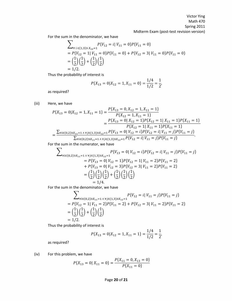
For the sum in the denominator, we have

∑ * + * + * +

* + * + * + * +

(

) (

) (

) (

)

Thus the probability of interest is

* +

as required?

(iii) Here, we have

* + * +

* +

* + * + * +

* + * +

∑ * + * + * + * + * +

∑ * + * + * + * +


∑ * + * + * + * + * +

* + * + * +

* + * + * +

(

) (

) (

) (

) (

) (

)

For the sum in the denominator, we have

∑ * + * + * + * +

* + * + * + * +

(

) (

) (

) (

)


* +

as required?

(iv) For this problem, we have

* + * +

* +



of 21

* +

* +

∑ * + * +


∑ * +

* +

* + * + * +

* + * + * +

(

) (

) (

) (

) (

) (

)


* + ( ) (

) (

) (

) (

) (

)

as required?

(v) No, this is not a 2-state homogeneous chain, because it is not homogeneous. Using the

diagram in Figure 6.1, we can see that

* +

* +

so that the probability of transitioning from 0 to 1 varies over time. Thus the chain is not

homogeneous, the Markov property fails.

midterm exam (post-test revision version) problem 1...

Documents