microrray image analysis with focus on background correction
TRANSCRIPT

Microrray image analysis with focus on Background correction
Zan LiSupervisor: Fons VerbeekLeiden Institute of Advanced Computer Science Leiden UniversityThe Netherlands
2
Abstract
Microarray technology is a new biotechnology, which allows the monitoring of expression levels for thousands of genes simultaneously. Image processing is an important aspect of microarray experiments, which will influence accuracy of subsequent analyses such as clustering or the identification of differentially expressed genes. To obtain meaningful information from the massive microarray images, it is needed to develop an algorithm, which can measure the expression levels of each gene. The process of identifying the spots, separating the foreground from the background and estimating the background intensity are known as gridding, segmentation, and background estimation.
This thesis presents one fully automatic gridding method based on low pass filter in the Fourier domain followed by threshold techniques. Segmentation techniques are explored; they are watershed operator and edge detector operator followed by seeded region grows. Comparing advantages and disadvantages of these two segmentation methods chooses watershed. Six background estimation methods are designed and implemented. Comparison of those background estimate methods is performed based on the results of each method.

3
Table of Content
Abstract.................................................................................................. 21. Introduction.................................................................................... 5
1.1 Motivation ....................................................................................................... 51.2 Identification of the Problems........................................................................... 51.3 Summary of Results ......................................................................................... 81.4 Organization .................................................................................................... 8
2. Microarray and Image processing background.......................... 92.1 Biological Background..................................................................................... 92.2 Principal of a cDNA Microarray Experiment.................................................. 102.3 Image Processing Background........................................................................ 11
2.3.1 Morphological operators and mathematic foundation............................... 122.3.2 Frequency filter ....................................................................................... 132.3.3 Watershed Segmentation ......................................................................... 152.3.4 Canny Edge Detector............................................................................... 15
3. Gridding........................................................................................ 173.1 Estimate Spot size .......................................................................................... 173.2 Preprocess ...................................................................................................... 18
3.2.1 Forming a combined image ..................................................................... 183.2.2 Preprocessing .......................................................................................... 18
3.3 Gridding......................................................................................................... 213.3.1 Gridding technique overview................................................................... 213.3.2 Our Gridding Approach........................................................................... 22
4. Foreground separation ................................................................ 294. 1 Foreground separation overview.................................................................... 294.2 Edge based method ........................................................................................ 314.3 Watershed Segmentation ................................................................................ 32
4.3.1 The multi-scale gradient algorithm .......................................................... 324.3.2 Preprocessing .......................................................................................... 34
4.4 Comparison of two segmentation methods ..................................................... 365. Background correction ................................................................ 39
5.1 Overview of background correction methods.................................................. 395.2 Morphological operators ................................................................................ 415.3 Our approaches of background correction ...................................................... 415.4 Background estimates analysis ....................................................................... 45
6. Data Analysis................................................................................ 496.1 Data Preprocessing......................................................................................... 49
6.1.1 Data transformation and filtering ............................................................. 496.1.2 Data Normalization ................................................................................. 50
6.2 General Data analysis..................................................................................... 526.3 Comparison of different background correction methods................................ 58
7. Conclusion and future work.......................................................... 61Bibliography........................................................................................ 63Acknowledgement.............................................................................. 66

4
Figure 1-1 Procedure of Microarray Experiment ........................................................ 7Figure 2-1 the Central Dogma................................................................................ 10Figure 2-2 Process of a Microarray Experiment ................................................. 11Figure 2-3 Microarray Image Sample....................................................................... 12Figure 3-1 Estimate Spot Size............................................................................... 17Figure 3-2 Remove noise procedure.................................................................... 19Figure 3-3 Image before removing noise .................................................................. 20Figure 3-4 Image after removing noise..................................................................... 20Figure 3-5 Main Framework of Subgrid Gridding .................................................... 22Figure 3-6 Original Profile & Profile after Low pass filter ................................ 24Figure 3-7 Profile after applying first threshold................................................. 24Figure 3-8 Profile after applying second threshold............................................ 25Figure 3-9 Profile after applying third threshold ............................................ 25Figure 3-10 Gridding result of Subgrids ............................................................. 26Figure 3-11 Framework of Spot Gridding........................................................... 27Figure 3-12 Spot Gridding Result ........................................................................ 27Figure 4-1 Illustration of separation using spatial concentric circular templates........ 29Figure 4-2 Canny Edge Detector Results without Preprocessing ..................... 31Figure 4-3 Canny Edge Detector Results after Preprocessing ................................... 32Figure 4-4 Preprocessing for watershed segmentation...................................... 34Figure 4-5 Watershed segmentation result ......................................................... 35Figure 4-6 Comparison of two segmentation methods' result………………………..37Figure 5-1 Illustration of different background correction methods…………………40Figure 5-2 Background trend after Opening Correction............................................ 43Figure 5-3 Background trend after Dilation-Erosion-Dilation................................... 44Figure 5-4 Background trend using quantile filter preceded by rank filter ….............45Figure 5-5 Histogram of Red Channel Background Estimates using Quantile…………Filter.............................................................................................................................46Figure 5-6 Histogram of Green Channel Background Estimates using Quantile Filter………………………………………………………………………………….46Figure 5-7 Background correction using different shapes of structuring element……………………………………………………………………………….47Figure 6-1 MA Plot showing different trend lines with or without normalization method..................................................................................................................... 51Figure 6-2 Red channel boxplot of foreground intensities among first 12 Blocks ..................................................................................................................... 53Figure 6-3 Red channel boxplot of foreground intensities among first 12 Blocks ..... 53Figure 6-4 Red and Green Channel Foreground Intensity Distribution of Whole Image................................................................................................................................ 54Figure 6-5 Circularity Histogram ............................................................................. 54

5
1.Introduction
1.1 MotivationThe discovery of microarray technology in 1995 has opened new avenues for investigating gene expressions and introduced new information problems [1]. Researchers have developed several tools for processing microarray image data, such as SPOT, QUANTARRAY and GENEPIX with the objective to extract biological meaningful information and conclusions.
The analysis of DNA microarray data consists of several steps [2] that can significantly deteriorate the quality of gene expression in formation, and hence decrease our confidence in any derived research results. Thus, microarray data processing steps become critical for performing optimal microarray data analysis and deriving meaningful biological information from microarray images.
Major work has been presented in the domain of microarray image analysis. Roberto Hirata JR et al.[3] introduces a technique using morphological operators to perform automatic gridding procedures for subgrids and spots. Buhler et al.[4]
describes a semi-automatic system which mainly focuses on the problem of finding individual spot with high accuracy. Jain et al[5] describes a system for microarray gridding and quantitative analysis that imposes different kinds of restrictions on the print layout. This method requires the rows and columns of all grids to be strictly aligned. For image segmentation, seeded region growing (SRG) algorithm, first introduced by Adams and Bischof [6] is adopted by researchers to segment microarray images. The software SPOT uses this segmentation technique. Jesus Angulo and Jean Serra [7] present Morphological segmentation by watershed transformation based on image operators derived from mathematical morphology.
However, although more and more scientists are using existing techniques to process microarray images, no universal consensus exists on how to design and analyze an experiment. There are always limitations for almost every developed algorithm. So it is worth doing further investigation on microarray image analysis. This thesis intends to improve techniques used in the current microarray image analysis procedure.
1.2 Identification of the ProblemsThe ideal microarray image has the following properties:A perfect image should only reflect measures of the fluorescence intensities for the dye of interest [15].
• All the subgrids are of the same size; • The spacing between subgrids is regular;• The location of the spots is centered on the intersections of the lines of the
subgrid;

6
• The size and shape of the spots are perfectly circular and it is the same for all the spots;
• The location of the grid is fixed in images for a given type of slides;• No dust or contamination is on the slide; • There is minimal and uniform background intensity across the image.
However, in the real world, almost no real microarray image meets all the above criteria. In fact, there are frequently observed variations on the spot position, irregularities on the spot shape and size, contamination such as undesired signals like photon noise, electronic noise, background fluorescence and global problem that affect spots. For detailed noise factor analysis, refer to Yoganand et al [18]. This makes image processing more challenging. Many algorithms and a lot of software exist for processing and analyzing microarray images. However, the existing software and algorithms for processing different microarray images exhibit all kinds of limitations. This thesis attempts to search for a universal technique, which is applicable to as many classes of images as possible.
The analysis of DNA microarray gene expression data involves two main areas [8]:
1. Image quantization2. Data analysis
Image quantization can be divided into four main steps:• Addressing or Gridding assigns coordinates to each spot in the image.
• Segmentation classifies pixels either as foreground-that is, as corresponding to a spot of interest, or as background.
• Background correction and estimation estimate background value to reduce bias of data.
• Information extraction includes calculating, for each spot on the array, red and green foreground fluorescence intensity pairs, background intensities, and related quality measures.
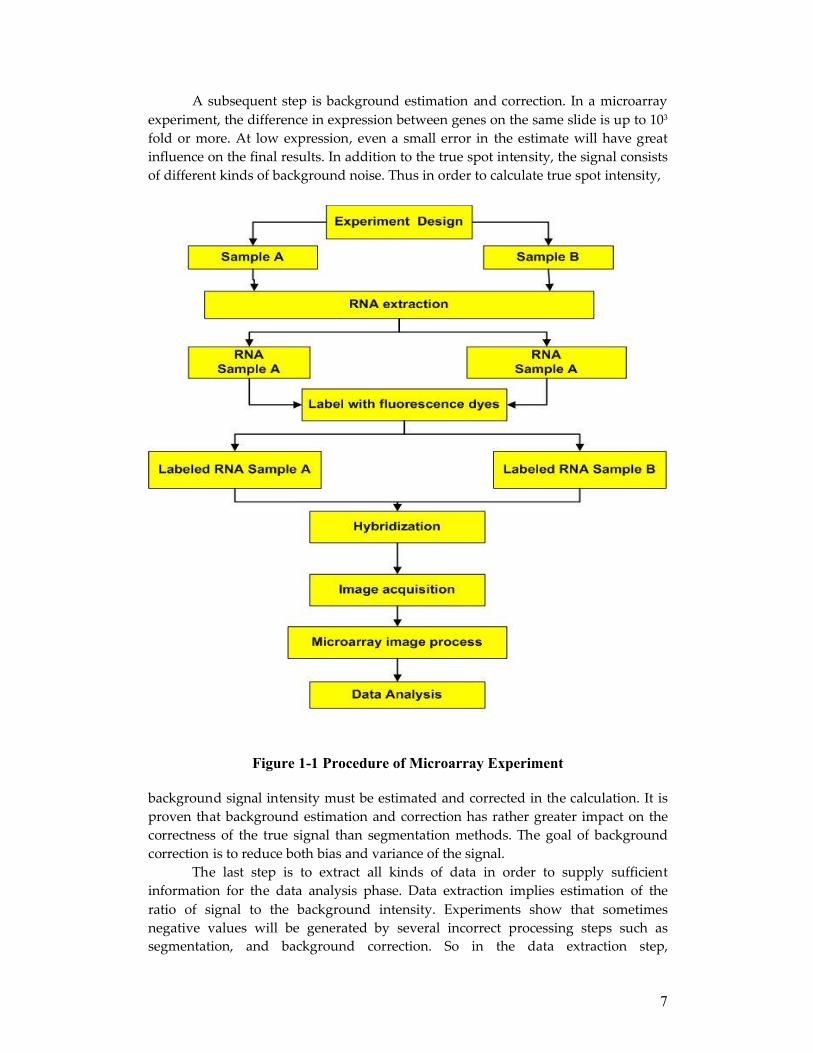
The overall flowchart of a whole microarray experiment is shown inFigure 1-1.
Many gridding algorithms developed so far still require users to locate spots, flag artifacts or reject faulty spots. Some existing software such as Spot, claims semi-automated or automated gridding but still requires intensive human intervention. The gridding technique used in this thesis is has not previously published (as far as we know). But this method yields high level of automation with high accuracy. We undertake in this thesis the implementation of automatic gridding technique without human intervention.
Segmentation is the second goal to achieve. Our primary concern is to identify a reliable measure with less user intervention. Two segmentation techniques are described in detail below.
7
A subsequent step is background estimation and correction. In a microarray experiment, the difference in expression between genes on the same slide is up to 103
fold or more. At low expression, even a small error in the estimate will have great influence on the final results. In addition to the true spot intensity, the signal consists of different kinds of background noise. Thus in order to calculate true spot intensity,
Figure 1-1 Procedure of Microarray Experiment
background signal intensity must be estimated and corrected in the calculation. It is proven that background estimation and correction has rather greater impact on the correctness of the true signal than segmentation methods. The goal of background correction is to reduce both bias and variance of the signal.
The last step is to extract all kinds of data in order to supply sufficient information for the data analysis phase. Data extraction implies estimation of the ratio of signal to the background intensity. Experiments show that sometimes negative values will be generated by several incorrect processing steps such as segmentation, and background correction. So in the data extraction step,

8
normalization strategies are necessary to ensure the correct results and global normalization is applied in this thesis.
1.3 Summary of ResultsThis study examines techniques for each step of the Microarray image analysis with focus on the background correction and estimation methods. One novel gridding method based on low pass filter for finding grid lines in Fourier domain is developed. This method was tested on eight different microarray images and gives correct results for eight images without any user intervention.
This study examines two segmentation methods: Watershed transformation and Canny Edge detector combined with Seeded region grow. Our implementation of Watershed transformation yields acceptable results for the experiment and doesn’t require user efforts. Canny edge detector yields quite interesting results compared to watershed segmentation. The circularity for each spot using canny edge detector is higher than that of watershed. Second advantage is that the canny edge detector saves computation cost. Furthermore, the number of missing spots would be considerably lowever than that of watershed method by choosing the correct parameters. However, one serious problem remains for canny edge detector. It requires great user efforts to find optimal threshold values for the canny edge detector on subgrid-based. So in the end, I chose watershed as segmentation method.
This study implements six different background correction methods and they are constant background correction, four-valley background correction, median filter background correction, opening background correction, Dilation-erosion-dilation background correction and quantile filter background correction. Quantile filter turns out to be the best choice in reducing bias and variance of background estimates among five different background correction methods.
In the end, different data is extracted from the image and is analyzed.
1.4 OrganizationThe rest of this thesis is structured as follows. After introducing some biological and image processing basics in chapter 2, in chapter 3, automatic gridding techniques are presented and compared. In chapter 4, we implemented the watershed transformation segmentation and explored the canny edge detector. Background estimation and correction methods are introduced in Chapter 5. In chapter 6, data extraction and analysis is discussed. In chapter 7, we summarize our conclusion and we discuss possible future direction and improvements.

9
2.Microarray and Image processing background
This chapter introduces biological concepts involved in microarray experiments to understand this thesis in section 2.1, Microarray images in section 2.2, and image processing techniques that are used in section 2. 3.
2.1 Biological Background
All living organisms consist of cells, which contain nucleic acids and proteins. Primary biological processes can be viewed as information transfer processes. The information necessary for the functioning of cells is encoded in molecular units called genes. Messages are formed from genes. Messages contain instructions for creation of functional structures called proteins.
This section reviews the basic information on proteins and nucleic acids and presents the fundamental mechanisms of cellular function.
DNA
DNA is composed of four basic molecules called nucleotides, which are identical except that each contains a different nitrogen base. Each nucleotide contains phosphate, sugar, and one of the four bases: Adenine, Guanine, Cytosine, and Thymine(Usually denoted A, G, C, T). The structure of DNA is described as a double helix.
Protein
Proteins are chains of smaller molecules, called amino acids joined by peptide bonds. The production of energy, the biosynthesis of all component macromolecules, the maintenance of molecular architecture, and the ability to respond to intracellular and extracellular stimuli, are all protein dependent.
The Central Dogma
The expression of the genetic information stored in DNA involves the translation of a linear sequence of nucleotides into a co-linear sequence of amino acids in proteins. The flow is shown in Figure 2-1:

10
Figure 2-1 the Central Dogma
The mechanism of living cells consists of four transformations monitoring the flow of information. The transformation from:
• DNA to RNA is called transcription.• RNA to DNA is called Reverse Transcription.• RNA to Protein is called Translation. • DNA to DNA is called Replication.
2.2 Principal of a cDNA Microarray ExperimentThe biological background explained in the previous section is the key element involved in microarray technology. In this section, we describe the motivation and the process of a microarray experiment.
Motivation
The knowledge of gene expression has applications ranging from basic research to applications such as diagnosing, staging and finding treatments of diseases. Traditional methods in molecular biology generally work on one gene in one experiment" basis, which means that the throughput is very limited and scientists can only be able to conduct such genetic analysis on a few genes at a time. Microarray technology makes it possible to measure the expression level of thousands of genes in a biological sample rapidly and efficiently on the slides. DNA microarray has attracted tremendous interests among individual genes.
Process of a cDNA Microarray Experiment
The process of a microarray experiment starts with the biologist’s hypotheses and selection a set of genes of interest, called target genes. DNA microarray is comprised of a library of genes, immobilized in a grid on a glass microscope slide called print-tip. Each unique spot on the print-tip contains a DNA sequence called control gene, derived from a specific gene that will bind to the mRNA produced by the treatment gene. This process is shown in figure 2-2.
The printing is made by an arrayer.

11
Figure 2-2 Process of a Microarray Experiment
There are six steps for creating a microarray image. First, two samples are taken from a living organism. Then cDNA from two samples is extracted. In the third step, cDNA is labeled with different fluorescence dyes. Fourth, two labeled samples are hybridized to a print-tip. The fifth step is to put control gene on target gene on the print-tip. Finally, scan the print-tip with two different wavelengths to produce two images from red and green channel using microscope.
Microarray image
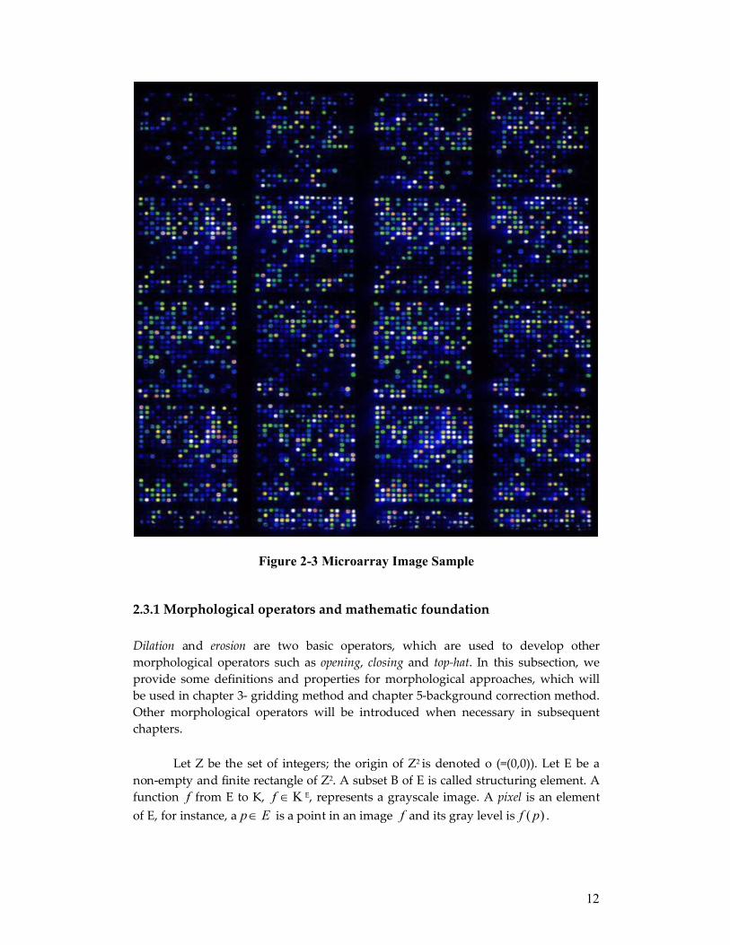
A typical microarray is showed in figure 2-3. Microarray image is composed of a matrix of equally spaced blocks called subgrid, each of which consists of the same number of rows and columns of spots. The spots in a subgrid are arranged in a relative uniform spacing with each other. They have a roughly circular shape.
2.3 Image Processing BackgroundThis section introduces some important image processing techniques involved in microarray image analysis to help readers understand this thesis.
12
Figure 2-3 Microarray Image Sample
2.3.1 Morphological operators and mathematic foundation
Dilation and erosion are two basic operators, which are used to develop other morphological operators such as opening, closing and top-hat. In this subsection, we provide some definitions and properties for morphological approaches, which will be used in chapter 3- gridding method and chapter 5-background correction method. Other morphological operators will be introduced when necessary in subsequent chapters.
Let Z be the set of integers; the origin of Z2 is denoted o (=(0,0)). Let E be a non-empty and finite rectangle of Z2. A subset B of E is called structuring element. A function f from E to K, K∈f E, represents a grayscale image. A pixel is an element of E, for instance, a Ep ∈ is a point in an image f and its gray level is )( pf .

13
The dilation and erosion of a function f by a structuring element B are, respectively, the functions δB(f) and εB(f) in KE given by , for any Ex ∈ ,
}:)(min{))((
}:)(max{))((
EByyfxfand
EByyfxf
xB
xB
∩∈=
∩∈=
ε
σ(2-1)
The operators opening and closing are denoted by Bγ and Bφ from KE to KE, given by BBB εδγ = and BBB δεφ = , are called, respectively, morphological opening and morphological closing by the structuring element B.
Let I be the identity operator. The operator i- Bγ is called opening top-hat by structuring element B.
Given a gray-scale image f : KE → , the horizontal projection profile of f , denoted by )( fPh
∑=∈
=kEyp
h pfkfP )(),0)(( (2-2)
We define the vertical projection profile of f , denoted by )( fPv , as the function from 0=yE to Z such that, for any 0)0,( =∈ yEk ,
∑=∈
=kEvp
pfkfPv )(),0)(( (2-3)
A regional minimum (resp., regional maximum) EM ⊂ of a function EKf ∈ is a connected component with a given value hpf =)( , Mp ∈∀ , such that
every point in the neighborhood of M has a strictly higher (resp., lower) value.
2.3.2 Frequency filterThis section will introduce frequency filter in Fourier domain, which will be used as a gridding technique in chapter three. Frequency filters process an image in frequency domain. The image is transformed using Fourier transformation, and then reverse transformed into real domain.
Fourier Transformation
The basic idea of Fourier transformation is to decompose an image into its sine and cosine components. The output of the transformation represents the image in the Fourier or Frequency domain. In Fourier space, each point in the image represents a particular frequency contained in the real domain image.
As we are only concerned with digital images in, we will restrict this discussion to the Discrete Fourier Transform (DFT).
The DFT is the sampled Fourier Transform and doesn’t contain all frequencies of an image, but only a set of samples, which is large enough to describe the real domain image. The number of frequencies corresponds to the number of pixels in the real domain image. For example, for an image with size NN × , the two-dimensional DFT is given by:

14
∑∑−
=
+−−
=
=1
0
)(21
02 ),(1),(
N
i
Nlj
NkjiN
jejif
NlkF
π(2-4)
Where ),( jif is the image in the real space and the exponential term is the basis function corresponding to each point ),( lkF in the Fourier space. The equation (2-4) can be interpreted as: the value of each point ),( lkF is obtained by multiplying the real image with the corresponding base function and summing the result.
The basis functions are sine and cosine waves with increasing frequencies, i.e. )0,0(F represents the DC-component of the image, which corresponds to the
average brightness and )1,1( −− NNF represents the highest frequency.
In a similar way, the Fourier image can be reverse transformed to the real domain. The inverse Fourier transform is given by:
∑∑−
=
+−
=
=1
0
)(21
02 ),(1),(
N
k
Nlj
NkjiN
lelkF
Njif
π(2-5)
Low pass filter
Low pass filter is a special type of frequency filter. The filter is based on Fourier transform. The operator takes an image and a filter function in the Fourier domain. This input image is then multiplied with the filter function in a pixel-by-pixel fashion:
),(),(),( lkHlkFlkG = (2-6)
Where ),( lkF is the input image in Fourier domain as explained above, ),( lkH is the filter function and ),( lkG is the output of the filter.
The form of filter functions determines basically three different kinds of filters: low pass filter, high pass filter and band pass filter. In this study, we use the low pass filter techniques to do gridding.
Low pass filter suppresses all frequencies higher than the cut-off frequency 0Dand leaves smaller frequencies unchanged:
>+
<+=
022
022
,0
,1),(
Dlkif
DlkiflkH (2-7)
In most implementations, 0D is given as a fraction of the highest frequency represented in the Fourier domain image.
15
2.3.3 Watershed SegmentationIn our proposed method in chapter four, watershed transformation yields the extracted spot information of microarray images. Watershed starts with the gradient of the image to be segmented. Intensity edges in the gradient image generally have high gradient values which appear as watershed lines, while the interior of each region, in this case spot, usually has a low gradient value which is considered as a catchment basin on the 3-D surface [9].
There are several ways to compute gradient images and they are Sobel operator, Prewitt operators and morphological gradient image.
Consider an image f -the result gradient image using one of the methods above, as a topographic surface and define the catchment basin of f and the watershed lines by means of a flooding process [10]. Imaging that we consider each minimum )( fM i of the topographic surface S, we plunge this surface into a lake with a constant vertical speed. The water entering through the holes floods the surface S. During this process, two or more floods coming from different minima may merge. We want to avoid this merge and build a dam on the points of the surface S where floods would merge. These dams define the watershed function f. They separate the various catchment basins )( fCBi , each one containing one and only one minimum )( fM i .
There are two important steps when performing watershed transformation. One is how to calculate gradient image from the input image to avoid problems such as over segmentation. Another is how to select minima or seed from each catchments basin. I will discuss these two aspects in the later implementation. This will be introduced in details in chapter four.
2.3.4 Canny Edge DetectorMost image segmentation approaches can be placed in one of five categories: clustering or threshold-based methods, boundary detection methods, region growing methods, shape-based methods and hybrid methods [11]. Boundary detection or edge-based methods focus on contour detection. The image is segmented based on spatial discontinuity or edge finding. This method is implemented as the convolution of mathematical gradient operators, or template matching operators, that use multiple templates at different orientations of the image. Sobel, Prewitt, Canny and Laplacian operators are examples of edge detection operators.
In this study, canny edge detector is used as one of segmentation methods in this study. In the following, here is how the canny edge operator works.
The canny edge detector takes gray image as input. First, it involves smoothing the image by convolving with a Gaussian filter.

16
Gauss filter:2
22
222
1),( σ
πσ
yx
eyxG+
= (2-8)
Finding the gradient of the image by feeding the smoothed image to a convolution operation with the derivative of the Gaussian in both vertical and horizontal directions in order to highlight regions of the image with high first spatial derivatives- edges in this case follows this. The convolution operation is described in the following equation 2-9.
∑∑−=−=
−−=⊗=N
Nl
N
NklykxIlkgyxIlkgyxI ),(),(),(),(),('
(2-9)
Where: ),( lkg = convolution kernel ),( yxI = Original image),(' yxI = Filtered image
2N+1 = size of convolution kernel
Instead of using a single threshold value for images, the Canny algorithm introduced hysteretic threshold, which is adaptable to the local content of the image [12]. There are two threshold levels, Th, high threshold and Tl , low threshold where Th
> Tl. Pixels with gradient values from convolved image above Th value are immediately classified as edges and otherwise set to zeros all pixels that don’t meet this criteria, a process known as non-maximal suppression. The algorithm track the edge contour, using two thresholds: Th and Tl . Neighboring pixels of edge contour pixels with gradient magnitude values less than Th , will still be classified as edges as long as their gradient magnitude values are above Tl. Tracking will then continues in both direction out from that point until the gradient magnitude value falls below Tl. This process alleviates problems associated with broken edges by identifying strong edges first and preserving the relevant weak edges, in addition to maintaining some level of noise suppression.
However, the performance of the Canny edge detector largely depends on the adjustable parametersσ , which is the standard deviation that controls the size of the Gaussian filter, and the threshold values Th and Tl . The bigger σ is, the larger the size of the Gaussian filter becomes, which introduces more blurring to the image, necessary for noisy image. However, the larger theσ , the less accurate is the edge localization. Smaller σ will also limits the blurring effect, maintaining finer edges in the image, which will introduce more noise in the image. The lower Th is, the more noise – faulty edges will be introduced in the images. Higher Th will exclude true edges. The same applies for the Tl .

17
3.GriddingA fundamental step of Microarray image analysis is the detection of the grid structure for the accurate location of each spot, representing the state of a given gene in a particular experimental condition. This step is known as gridding. In this chapter, we will give a brief overview about current gridding techniques and then, we will propose our gridding method.
3.1 Estimate Spot sizeThere will be several steps ahead, which should be performed to ensure high success rate of gridding result such as removing noise in the image. Morphology operators are applied to remove noise in the image with proper structuring element size, which is highly correlated with the size of each spot. Estimating the average spot size is the first step.
The average spot size of microarray image is obtained by applying morphological operator, erosion with increasing circular structuring element with radius from 1 to 20 pixels. Intensity values of whole image are summed up iteratively after applying erosion with increasing structuring element. The difference between two sums of intensity value with sequential number of structuring element size is calculated. The structuring element size, where corresponding difference of two sums calculated above is maximal, is taken as the average size of all spots. In Figure 3-1, after structuring element size five (x is approximately equal to five), the different between two adjacent sums remain roughly a constant value. Thus five is taken as the average radius of all spots on the slide.
Figure 3-1 Estimate Spot Size

18
3.2 Preprocess
The input to the image analysis procedure is a critical element to the results. Thus before performing subsequent image analysis such as gridding and segmentation, we need to preprocess the input image.
3.2.1 Forming a combined image
The images being used by the image analysis procedure consists of a pair of unsigned 16-bit images, which are storedin TIFF format files. We name these images “ R ” and “G ” for red and green images, with R corresponding to the dye 5Cy and G to 3Cy . Both the gridding and segmentation stages require a single image due to computational cost. This image should not be dominated by either of the two inputs. In other words, R and G images should contribute equally in the combined image. The following processing is used to produce a 16-bit combined image, RG and achieve these aims.
Form an combined image:
1. Median values are computed: );();( GmedianmRmedianm GR ==
2. An initial combination is computed as:
RmmG
R
G •+
3. Finally half of the value computed above is taken as combined image
Subsequent image analysis procedures such as gridding and segmentation use this combined image as input image.
3.2.2 Preprocessing
Preprocessing of combined image is necessary to gridding to ensure good result. Typically, a microarray image takes into account many disturbing factors such as spot morphology, signal strength, background fluorescent noise, and shape and surface degradation [18]. Noise factors [18] and their interactions will significantly deteriorate the ability to accurately detect true gene-expression signal. Thus, it’s necessary to understand the noise factors and find a solution to remove noise. There is detailed information about noise factors in [18].

19
Figure 3-2 Remove noise procedure
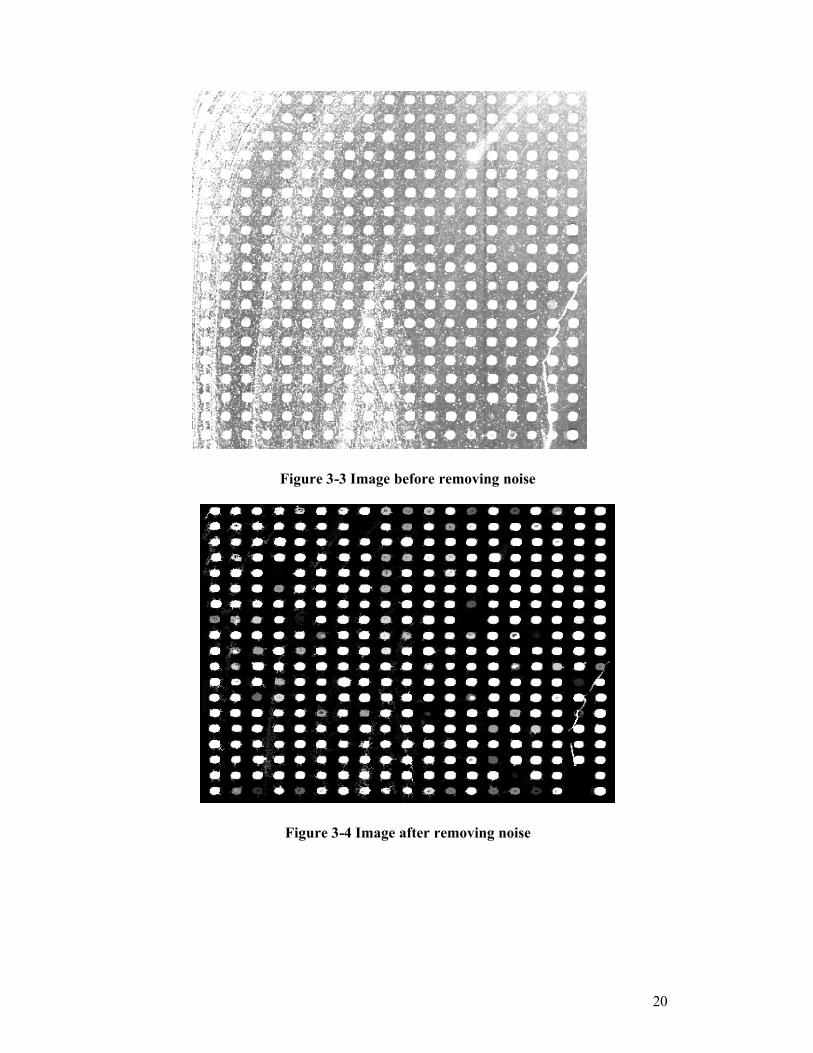
The whole process of removing noise is shown in Figure 3-2. First erosion operator with structuring element larger than two times of the average spot size is applied to remove foregrounds spots. Then apply image reconstruction to the result background. An image with less noise is obtained by subtracting result background from original image. This is mainly to remove large flare noise. After that, opening operator with structuring element smaller than spot size is applied to remove small spikes in the image. Apply image reconstruct again to the result image.
Figure 3-3 shows original noisy image before performing noise reduction. Figure 3-4 is the cleared image after performing noise removal steps introduced above. You can see clearly how noise removal makes the subsequent step- Griddingeasy.
20
Figure 3-3 Image before removing noise
Figure 3-4 Image after removing noise

21
3.3 Gridding
3.3.1 Gridding technique overview
This section will introduce existing gridding methods. Grid alignment techniques can be viewed in terms of automation as manual, semiautomatic, and fully automated [17].
Manual grid alignment methods
A user specifies dimension of a grid template and a radius of each spot to form a template. Computer user interfaces are available for adjusting the predefined grid template to match the microarray spot layout. The advantage of this method is that one could possibly obtain ‘perfect’ grid alignment by providing human computer interface software tools that are built for adjusting shape and location of each spot individually. However, disadvantage of this method is obvious. This approach for grid alignment is not only very time consuming and tedious, but also almost impossible to repeat or use for high-throughput microarray image analysis. So efficiency and full automation are the goals for grid alignment.
Semiautomatic grid alignment methods
This approach can perform grid alignment by computer and also allows user to intervene in order to achieve correctness of gridding result. The benefits of semiautomatic grid alignment method include reduction of human labor and time. Nevertheless these methods might not suffice to meet requirements of high throughput of microarray image processing.
Fully automated grid alignment methods
These approaches should reliably identify all spots without any human intervention based on one-time human setup. Most of the times, the challenging of designing fully automated grid methods is to identify all parameters that represent prior knowledge and quantify constraints for those parameters. Typically these methods are data-driven.
Roberto Hirata JR [3] introduces morphological operator in gridding. Michele Ceccarelli [13] developed a deformable grid matching which generates a grid hypothesis based on Radon Transformation and accounts for local grid deformations. Guiliano Antonio [16] reports an approach based on Markov Radon field for the automatic gridding. These approaches are all claimed to be fully automatic approach.

22
In this thesis, a novel gridding method was developed, which is fully automated.
3.3.2 Our Gridding ApproachIn this section, we will propose a novel gridding method based on Fourier domain. We use subgrid gridding to differentiate with spot gridding because spot gridding uses different method.
Subgrid gridding
Figure 3-5 shows the main framework of subgrid gridding.
Figure 3-5 Main Framework of Subgrid Gridding

23
Subgrid Gridding Steps:
1. Gauss filter with 4=σ is applied to blur image, which is used to eliminate regional minima (refer to chapter 2-section 2.3.2) of projection profile between spots.
2. Sum up the intensities across pixels in each row and each column to get row and column profile separately.
3. Transform row and column profile to frequency domain (Apply Fourier transformation to row and column profile).
4. Apply low pass filter in frequency domain with cut-off frequency =2/3 (Refer to equation 2-6 and 2-7).
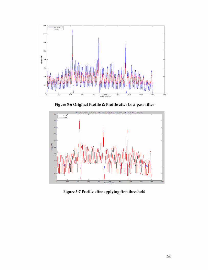
5. Apply inverse Fourier to transform image back to spatial domain. The profile in y direction is shown in Figure 3-6. The red curve is the profile after low pass filter and the blue curve is original profile.
6. Subtract result profile from original profile, and result is denoted by diff(i),where i is coordinate.
7. Calculate average value of diff(i),denoted by thresh1. 8. Apply first threshold to the profile. Assign pixels with diff (i) <1.4*thresh1 with
the minimum intensity value in the original profile. The effect of this threshold is to retain minima of original profile in the resulting profile. The profile is shown in Figure 3-7. The regional minima in blue curve in the Figure 3-7 are replaced by regional minima in red curve.
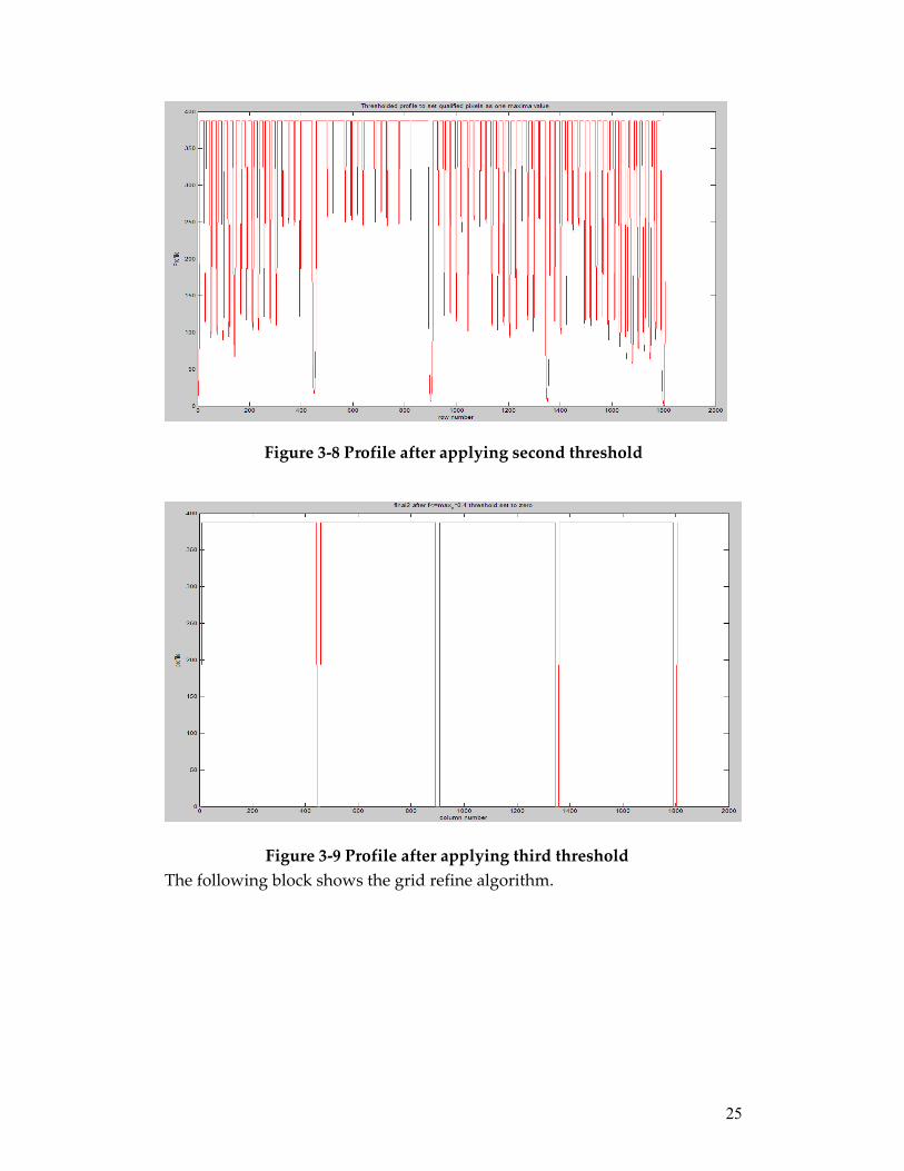
9. Apply second threshold to the profile. Assign pixels with diff > thresh2 with the maximum intensity in the original profile. The effect of this threshold is to retain maxima of original profile in the resulting profile. The profile is shown in Figure 3-8. The regional maxima are replaced by one intensity value, the maximum intensity value in the original profile.
10. Apply dilation to close small valleys to exclude regional minima between spots.
11. Apply third threshold with threshold value thresh2 = 0.3 * max_y, max_y is the maximum value in the current profile. Assign pixels with intensity value less than thresh2 with zero and the rest with maximum intensity value in the profile. The profile is shown in Figure 3-9.
12. Find gridlines where intensity value = 013. Apply Grid Refine algorithm introduced by Yu Luo [15].
24
Figure 3-6 Original Profile & Profile after Low pass filter
Figure 3-7 Profile after applying first threshold
25
Figure 3-8 Profile after applying second threshold
Figure 3-9 Profile after applying third thresholdThe following block shows the grid refine algorithm.

26
Real Refine_Grid(P)1. ←Rnew average distance between adjacent cells on P
2. repeat 3. RnewR ←4. PP ←'5. repeat
6. ←d distance between a pair of adjacent lines7. if Rd α> then remove a line from 'P8. if Rd α> then add a line to 'P9. until all lines have been considered10. ←Rnew average distance between adjacent cells on 'P11. until RRRnew γ≤− ||12. return R
Figure 3-10 shows the gridding result. This gridding method was tested on eight different microarray images and all yield correct results.
Figure 3-10 Gridding result of Subgrids
Spots Gridding
Spot gridding is much easier than subgrid gridding. The Figure 3-11 shows basically the main framework of spot gridding.

27
Projection to get row and column profile
Apply top-hat operator
Clear Image Border noise
Find regional minima of one profile
Apply Spot Refine algorithm
Figure 3-11 Framework of Spot Gridding
First, apply top-hat morphological filter to subgrid to remove noise that will affect accurate gridding. The image after top-hat is shown in Figure 3-12. Clearing noise from subgrid border is to precisely find the first and last spot lines, which are highly unreliable due to noise. Spot Refine algorithm is the same as grid refine algorithm introduced above. The gridding result is shown in Figure 3-12..
Figure 3-12 Spot Gridding Result

28
This gridding method is a novel method, which is not documented in anyproceedings. Image is transformed into Fourier domain to apply low pass filter. After transforming image back to spatial domain, it explores characteristics between original profile and resulting profile and several threshold techniques are used according to these characteristics. This novel method was tested on several microarray images and proven to yield results with high success rate and throughput. Furthermore, this method probably leaves space to develop different thresholdtechniques to yield even better results.

29
4.Foreground separation Following outcome from chapter three-gridding, a spot location is a rectangular image enclosing one spot, denoted by a grid cell. The subsequent task is to classify pixels that belong to foreground, denoted by spot signal and background. Usually some scientific papers refer to this task as segmentation. In this thesis, we name it foreground separation because it involves image segmentation and another foreground separation technique clustering.
In this chapter, after giving an overview of foreground separation methods, we will discuss about techniques used in our research to separate foreground.
4. 1 Foreground separation overview
The term image segmentation refers to the problem of partitioning an image into spatially contiguous regions with similar properties, e.g. intensity, color, while the term image clustering is associated with grouping together set of pixels with similar properties not necessarily spatial connected. Based on this concept, foreground separation methods can be roughly categorized into the following: (1) spatial template, (2) intensity-based clustering, (3) intensity-based segmentation, (4) spatial and intensity information [17].
Spatial template
This foreground separation method consists of two concentric circles, where the pixels inside the smaller circle are labeled as foreground and the pixels outside of the larger circle are labeled as background (see Figure 4-1). All pixels between two concentric circles are considered as unreliable pixels, which will not be used in calculation later. Apparently, this technique ignores the fact that spots have varying radius, irregular shapes beside circle, and offsets from the grid cell center. Thus, spatial template technique will yield poor foreground separation, which will lead to increased background level and distorted signal-to-background ration. ScanAlyzesoftware uses this technique. A quantitative comparison of the results obtained from circular spots and segmented spots can be found in [5].
Figure 4-1 Illustration of separation using spatial concentric circular templates

30
Foreground separation using intensity-based clustering
This type of technique uses image threshold techniques, which choose a threshold intensity value and assign the signal label to all pixels that are above the threshold value (or below). The threshold value can be chosen by computing the expected percentage of foreground pixels inside a grid cell based on the knowledge about image resolution and spot radius. Several clustering approaches use this intensity-based technique, such as K-mean or K-medoids.
The main advantage of this method is simplicity. However, there is a major disadvantage of this technique. It ignores large difference of intensity values within a spot. Thus this technique will fail in classifying pixels accurately as foreground or background pixels. The resulting foreground pixels (spot signal) might not be connected with each other. The resulting foreground mask using this technique probably excludes pixels, which belong to foreground due to their low intensity values, and includes pixels with high intensity values, which belong to background.
Foreground separation using intensity-based segmentation
Seeded region growing and watershed segmentation fall into this category. Seeded region growing (SRG) starts a set of input pixels called seeds. SRG group’s pixels with similar intensities with the seeds to form a set of contiguous pixels, called region until all pixels have been assigned to one of the regions grown from the initial seeds. In case of Microarray images, the foreground seeds can be chosen either as the center of a grid cell or as the pixel having maximum intensity value inside a grid cell. Similarly the background seed could be selected either as four sides of a grid cell or the pixel with minimum intensity value inside a grid cell. Software SPOT uses this segmentation technique.
Besides difference mentioned in this section, another main difference of segmentation approach with clustering is that it exclude dark pixels from the foreground assuming that they are surrounded by a connected set of pixels. In contrary, the clustering approach will include pixels belonging to the background to the foreground cluster. Another issue to consider is that choosing the most appropriate seeds introduces difficulty to this approach. But in the case of Microarray image, it is much easier to choose seeds as we discussed above.
Foreground separation using spatial and intensity information
This technique is hybrid method, which consist of segmentation or clustering image partitions, spatial template image partitions, statistical testing, and foreground/background trimming.
Mann-whitney statistical testing and spatial and intensity trimming belongs to this technique.

31
4.2 Edge based methodAccording to pros and cons of different separation methods introduced in previous section, watershed segmentation is chosen for our implementation. Alternativesegmentation method- canny edge detection is briefly explored to provide reference for further investigation on segmentation methods.
Edge detection is a basic technique used in most image processing applications to obtain information from frames as precursor step to feature extraction and object segmentation. This process detects boundaries between objects and background in the image. The basic edge-detection operator is a gradient operation such as Roberts, Prewitt, and Sobel operators. Refer to section 2.3.4 for detailed information.
Before applying canny edge detection algorithm, preprocessing is necessary. Figure 4-2 shows segmentation result without applying preprocessing. You can see from the image that noise dramatically affects precise edge location.
Figure 4-2 Canny Edge Detector Results without Preprocessing
In the following, here are the steps of preprocessing:

32
Preprocessing for Canny edge detector:
1. Clear noise on the image border. 2. Fill holes in the spot to exclude false edges inside spot. 3. Reconstruct the image.4. Apply morphological operator “erosion” with circular structuring
element to remove small bright dot with circle diameter less than three.5. Reconstruct the image.6. Apply canny edge detector with two threshold values: 0.453 and 0.931.
Figure 4-3 shows the result of canny edge detector with preprocessing applied. As you can see from this figure, the segmentation result is quite good.
Figure 4-3 Canny Edge Detector Results after Preprocessing
4.3 Watershed Segmentation
Watershed transformation is a powerful tool for image segmentation. However, the effectiveness of the watershed segmentation method is limited by the quality of the gradient image used in the methods. Over-segmentation is a typical problem.
In the following two subsections, conventional approach of watershed segmentation is introduced and disadvantages are analyzed first. Then a modified algorithm of watershed segmentation is proposed for eliminating irrelevant minima in the resulting gradient image [9].
4.3.1 The multi-scale gradient algorithm
Conventional Approach

33
A conventional gradient operator, such as the first partial derivative of Gaussian filter and morphological gradient operators produces too many local minima because of noise within homogeneous regions. Each minimum of the gradient introduces a catchments basin within the watershed transformation, which results in over-segmentation problem, e.g. a homogeneous region may be partitioned into a large number of regions and proper edges are lost in a multitude of false ones. One approach to deal with this problem is to threshold the gradient.
However, conventional gradient operators produce low gradient values at blurred edges, even though the intensity change between the two sides of an edge may be high. Thresholding cannot eliminate the local minima caused by noise and quantization error while preserving those produced by blurred edges. Another solution for this problem is to extract markers and impose them on the gradient image, which may require prior knowledge about objects and background to be segmented. After watershed segmentation, region merging is usually performed to further remove false contours [20]. This process may be computationally expensive than watershed transformation because too many catchments basins have to be merged, which greatly decreases the speed of the entire segmentation method.
Proposed Approach
In this thesis, we propose a multi-scale gradient algorithm based on morphological operator for watershed-based image segmentation [9]. This algorithm efficiently enhances blurred edges while being very robust to multi-edge interactions. This increases the gradient value for blurred edges above those caused by noise and quantization error. We present an algorithm to eliminate the local minima produced by noise and quantization error.
The morphological gradient operators can be described as )()()( BfBffG Θ−⊕= (4-1)
Where ⊕ andΘ denote dilation and erosion [21]. Its performance depends on the size of structuring element B. Usually large structuring element results in serious interaction among edges which may lead to gradient maxima not coinciding with edges, called over segmentation. However, if it is too small, this gradient operator produces a low output values for edges, called under segmentation. Proper choice of structuring element is crucial for the performance of watershed segmentation.
In order to avoid both over-segmentation and under-segmentation problems caused by the size of structuring element, a multi-scale morphological gradient algorithm was proposed [9]. In the following, here is how multi-scale algorithm works.
Let structuring element iB ,2
0 spotsizei ≤< , denote a group of circular
structuring elements. The size of iB is circular disk with radius i , i.e. 0B is a circle
with radius 1 and 1B is a circle with radius 2 until iB reaches2
spotsize . The multi-
scale gradient is defined by

34
( ) ( )( )[ ]∑ −− ΘΘ−⊕= 111)( iii BBfBfn
fMG (4-2)
This operation-equation 4-2 produces spot edges with the width of two pixels. In practice the outcome is more robust to noise due to the averaging operation used in the algorithm. The location of gradient maxima-edge in this case is not disturbed by the presence of other edges.
4.3.2 Preprocessing
There are two images, red and green scanned at different wavelength. Watershed segmentation is computation expensive algorithm. So it is not recommended to segmentation both images at the mean time. In order to keep information from both channels, there are two approaches to form an image as an input to segmentation. The first one is always taking the larger intensity values from two images at the same position to form an image. However, this approach will introduce more noise into the combined image, which makes preprocessing much harder. Furthermore, this image should not be dominated by either of the two images-that is raw images Rand G should contribute equally in the combination.
Figure 4-4 Preprocessing for watershed segmentation
Second approach uses the combined image introduced in section 3.2.1 as input image. The combined image is processed for noise reduction. In the following figure, it describes the process of noise reduction for one spot at a time.

35
In the figure 4-5, segmentation result for watershed transformation is shown.
Figure 4-5 Watershed segmentation result
According to classical paradigm of morphological segmentation [22] (Beucher, 1999), the algorithm for segmenting the spot is as follows:

36
Morphological Segmentation Procedure:1) Define the gradient function to be flooded using multi-scale gradient
operator introduced above, referring to equation (4-2). 2) Obtain two markers:
The outer markers are the filled borders of the bounding box of spot, first row and column, and last row and column, denoted by omk . For the inner markers, denoted by imk , we propose an algorithm. The procedure for each spot i is the following
a. Applied Otsu's threshold method to spot i , which chooses the threshold to minimize the intraclass variance of the thresholded black and white pixels.
b. Calculate number of ones in the binary image which is obtained from step above. Put them in an array named )(iN , which i is the index for the spot and N is the number of ones in the binary image-bounding box of spot i .
c. The total number of ones inside this bounding box of spot i• 0)( =iN : The spot i is classified as absent spot and no
marker inner is assigned for foreground. • 1)( =iN : The spot i is classified as clear spot and the
inner marker is defined where ‘1’ appears. • 1)( >iN : The spot i is classified as vague spot. Shrink the
binary image to point with one ‘1’. The inner marker is defined at this point.
3) Construction of watershed line for )''( fg + associated to inner and outer markers of the spot-bounding box is: ),,( emkimkgWatershedWshedLine = , where WshedLine is the line boundary of each spot.
4.4 Comparison of two segmentation methods
In this section, brief comparison of two segmentation methods, watershed segmentation and canny filter is given.
First, we will give some advantages for canny filter. Figure 4-6 shows the segmentation results using watershed and canny filter for one spot. For further compassion, you can refer to figure 4-3 for canny edge result and figure 4-5 for watershed segmentation applied on the first Subgrid of the image. Figure 4-5 and Figure 4-6 shows results for one subgrid using watershed and canny filter. As we probably notice that, the shape obtained using canny filter is much circular than that obtained using watershed. Circularity is one criterion used to evaluate the quality of segmentation results. Another thing for canny filter is that computation complexity is much lower than that of watershed transformation. According to experiment, the time that Canny edge detection cost to process one subgrid is roughly five seconds while watershed segmentation took roughly one minutes 35 seconds to finish the same subgrid. This is because we feed the whole subgrid image to the canny filter

37
and in the end we get all the results for one sub-grid. However, for watershed segmentation, we have to iterate each spot to apply watershed, which increase computation complexity.
Result of Watershed segmentation result of Canny Filter
Figure 4-6 Comparison of two segmentation methods' result
However, except those advantages of canny filter. We have one important problem that needs to be paid attention, and that is tuning of two threshold values of canny filter, referring to section 2.3.4. Several tests on the selection of two threshold values of canny filter were performed. One result for two threshold values is:
1. The higher threshold value is 931.0=highT .
2. The lower threshold value is 453.0=owlTYou probably notice that the precision of two threshold values reaches to three digits after decimal. Furthermore, for different sub-grid image, user has to manually adjust these two threshold values until the optima one is found. This requires lots of manual work, which is not recommended at all. So according to analysis, canny filter method is not chosen as final segmentation method.

38

39
5.Background correction The motivation for background correction is the belief that a spot’s measured intensity includes a contribution especially due to the hybridization of the target to the probe, for example, various kinds of noises. In order to obtain an estimate of the true spot intensity it is almost universal to subtract the background estimate from the foreground estimate.
This chapter will introduce background correction and estimation methods implemented in this thesis. Section 5.1 gives an overview of existing background estimation methods. Section 5.2 introduces several important image analysis techniques that will be used in background correction methods. Section 5.3 introduces six background correction and estimation methods.
5.1 Overview of background correction methodsAfter detecting the location, size, shape of each spot using watershed segmentation, we thus need to calculate foreground and background intensities, and possibly spot quality measures.
We define the foreground intensity as the mean or median of pixel values within the segmented spot mask, which is also used by most Microarray analysis packages. However, more various methods exist in the choice of background correction and estimation methods. Basically, background methods can be classified into four categories and they are:
• Local background • Morphological opening• Constant background• No Adjustment
Local background
One choice for the local background is to consider all pixels that are outside the spot mask but within the bounding box centered at the spot center. Such a method is implemented by ScanAlyze [23]. This is represented as the blue rectangular in Figure 5-1. The median of values in selected regions surrounding the spot mask is then used as an estimation of local background intensity (GenePix [24], ScanAlyze [23], QuantArray [25]). However, because this method takes into consideration the boundary pixels immediately surrounding the spots edges, the background estimate is more sensitive to the performance of the segmentation procedure.
One of the background adjustment methods implemented in QuantArray [25]
considers the area between two concentric circles, such as the green circles in Figure 5-1. By not considering the pixels immediately surrounding the spots, the background estimate is less sensitive to the performance of the segmentation.

40
Spot [27] considers the four pink diamond-shaped areas in Figure 5-1(A). These pink regions are referred to as the valleys of the array and have the furthest distance from all four surrounding spots. The local background for each spot can be estimated by the median of values from the four surrounding valleys. The advantage of this method is somewhat independent of the segmentation results. Using valley pixels, which are very distant from all spots, ensures to a large degree that the background estimate is not corrupted by pixels belonging to a spot or a spot boundary. Such corruption by bright pixels may occur in the other methods.
(A) (B)
Figure 5-1 Illustration of different background correction methods [26]
Morphological operators
Our preferred approach to background correction relies on non-linear filter called morphological filters such as opening, erosion, dilation and rank filters. See Soille[29]
for a detailed description. These methods will be introduced in details in section 5.3.
Constant background
This method subtracts a constant background for all spots on the slide. This is a global method, which subtracts a constant background for all spots on the slide. However, constant background correction method ignores the variability of background estimates among individual spots, which will yield incorrect signal estimates.
No adjustment
We consider the possibility of no background adjustment at all.

41
5.2 Morphological operatorsThis section gives definitions and important properties of rank filter and quantile filter [28], which will be used for background correction.
Rank filters
A gray-scale image can be represented by the image function: ff TDf →: ,with
domains 2Ζ⊂fD , and ℜ∈fT or Ζ∈fT depending on if the gray levels are continuous or discrete, respectively. That is, )(xf is equal to the gray level at position ),( jix = . Let B be a compact subset of Ζ that is symmetric with respect to its origin. A rank filter )(, fkBς of order k using a structuring element B positioned at pixel x and operating on f is defined by
};|)({)))((,( BxDxxxxfrankxf BfBBkkB ∈∈−−=ς , (5-1)
Where )(xrankk
equals the thk element of a x sorted in ascending order. It holds that
nBBB ,2,1, ...... ςςς <<< , (5-2)
Where )(Bcardinaln = equal the number of pixel inside B that is the size of the filter mask.
Quantile filters
A special case of rank filtering is obtained if rank is defined as a fraction of the number of pixels inside the structuring element. This is called a quantile filter and is denoted }{, qBς where the rank is defined by
=<<+×
=1),(
10|,1)(|}{
qBcardinalqqBcardinal
q (5-3)
with || x equals to the greatest integer less than or equal to x.
5.3 Our approaches of background correction This section discusses background correction methods that were implemented in this thesis. Detailed comparison of those background correction methods will be given in chapter 6 data analysis.
Constant background
This constant background chose the 5th percentile of the whole image intensity values in ascending order as background estimate for all spots on the slide.
Local background

42
There are two local background methods implemented in this thesis. One method is four squares, which is adopted from four valleys [26]. This method uses four red squares with side length 3x3 starting from each vertex of spot rectangular box shown in figure 5-1 (B).
Another local background correction method considers as background estimates all pixels that at not within spot mask but are within a square centered at the spot center. This region is represented by region within blue dotted square and red circle shown in figure 5-1 (A). Median value of pixels intensities within this region is used as background estimate.
Morphological operators
In this category, three different morphological operators are used to estimate local background and they are opening combined with small dilation, dilation-erosion-dilation, rank filter combined with quantile filter.
Morphological opening preceded by small dilation with square structuring element of size 3x3 is applied to the original images R and G using a rectangular structuring element with side length at least two and half times as large as spot separation distance[26],which is the distance between the centers of adjacent spots in a column or in a row; This method consists of the following steps:
Morphological opening followed by small dilation:
1. Dilation: Bδ , B is square structuring element with side length equal to three. 2. Opening: Bγ , B is rectangle-structuring element with height equal to two
times and a half of vertical spot separating distance and width equal to two times and a half of horizontal spot separating distance.
3. Median value of result background for each spot is taken as background estimate.
This operation removes all the spots and generates an image, which is an estimate of the background for the entire slide. For individual spots, the median value is taken as background estimate for each individual spot.
Morphological opening results in lower background estimates than other simpler methods. More importantly, morphological background estimation is expected to be less variable than the other methods, because spot background estimates are based on pixel values in a large local window, and yet are not corrupted by brighter pixels belonging to the edge of spot signal.
43
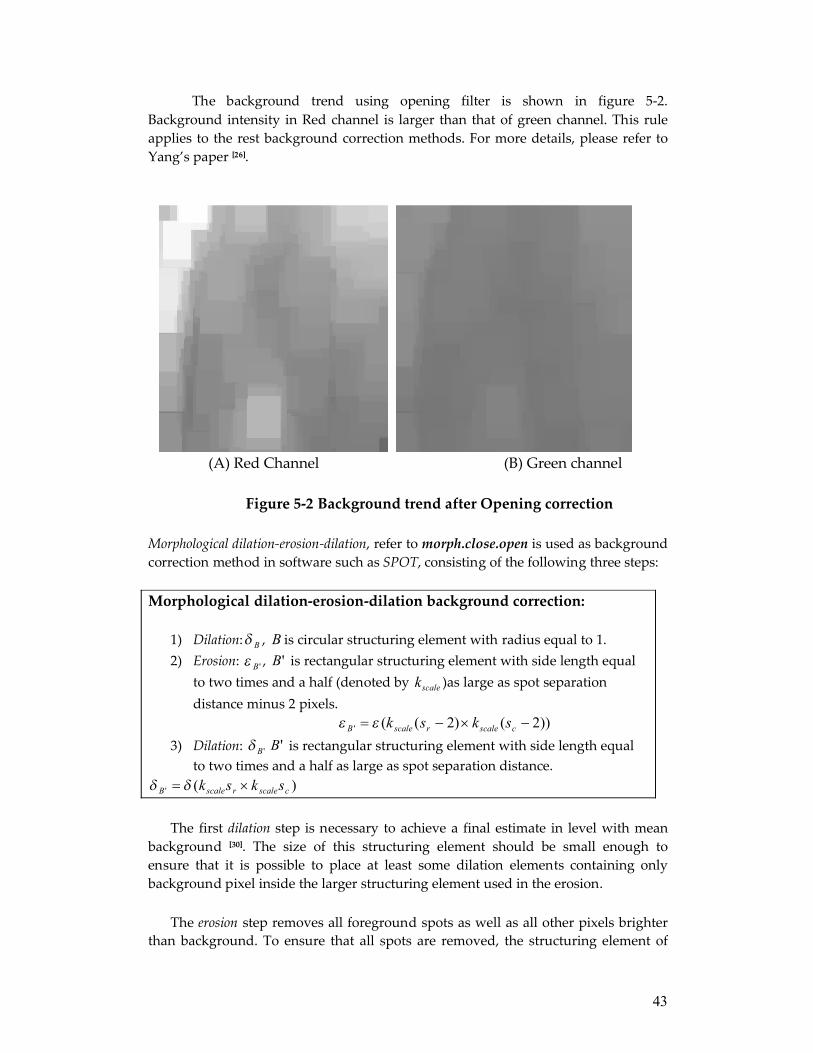
The background trend using opening filter is shown in figure 5-2. Background intensity in Red channel is larger than that of green channel. This rule applies to the rest background correction methods. For more details, please refer to Yang’s paper [26].
(A) Red Channel (B) Green channel
Figure 5-2 Background trend after Opening correction
Morphological dilation-erosion-dilation, refer to morph.close.open is used as background correction method in software such as SPOT, consisting of the following three steps:
Morphological dilation-erosion-dilation background correction:
1) Dilation: Bδ , B is circular structuring element with radius equal to 1. 2) Erosion: 'Bε , 'B is rectangular structuring element with side length equal
to two times and a half (denoted by scalek )as large as spot separation distance minus 2 pixels.
))2()2((' −×−= cscalerscaleB skskεε3) Dilation: 'Bδ 'B is rectangular structuring element with side length equal
to two times and a half as large as spot separation distance.)(' cscalerscaleB sksk ×= δδ
The first dilation step is necessary to achieve a final estimate in level with mean background [30]. The size of this structuring element should be small enough to ensure that it is possible to place at least some dilation elements containing only background pixel inside the larger structuring element used in the erosion.
The erosion step removes all foreground spots as well as all other pixels brighter than background. To ensure that all spots are removed, the structuring element of
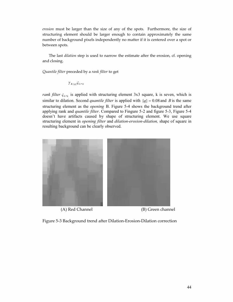
44
erosion must be larger than the size of any of the spots. Furthermore, the size of structuring element should be larger enough to contain approximately the same number of background pixels independently no matter if it is centered over a spot or between spots.
The last dilation step is used to narrow the estimate after the erosion, cf. opening and closing.
Quantile filter preceded by a rank filter to get
kbqB ,}{, ςγ
rank filter kb ,ς is applied with structuring element 3x3 square, k is seven, which is similar to dilation. Second quantile filter is applied with 08.0}{ =q and B is the same structuring element as the opening B. Figure 5-4 shows the background trend after applying rank and quantile filter. Compared to Fingure 5-2 and figure 5-3, Figure 5-4 doesn’t have artifacts caused by shape of structuring element. We use square structuring element in opening filter and dilation-erosion-dilation, shape of square in resulting background can be clearly observed.
(A) Red Channel (B) Green channel
Figure 5-3 Background trend after Dilation-Erosion-Dilation correction

45
(A) Red Channel (B) Green channel
Figure 5-4 Background trend using quantile filter preceded by rank filter
5.4 Background estimates analysis In this section, we will show background estimates results
Spatial trend
The following figure shows the estimated background on images from both channels for the first subgrid. A spatial trend of the background intensity is clearly visible, and the pattern of this trend is different in the red and green channel. Usually background intensity of red channel is higher than that of green channel. The background intensity trend of other subgrids is similar.
Pixel distribution
Another property of background pixels is that their distributions are different in the two channels.

46
Figure 5-5 Histogram of Red Channel Background Estimates using Quantile Filter
Figure 5-6 Histogram of Green Channel Background Estimates using Quantile Filter
Among those different background correction methods, morphological background correction results in smaller background estimates than another three methods. Furthermore, it is less variable than other methods. It is claimed that quantile filter has variability 3 times lower than morphological operators such as opening. It was examined that morphological opening has a mean bias between -47 and -248 compared to a bias between 2 and -2 for the rank filter [28]. Furthermore, from the figures above, quantile filter preceded by small rank filter yield smooth background compared to other two morphological methods. Detailed data comparison will be given in chapter 6.
47
However, accuracy of these morphological methods depends heavily on the size of structuring element. Detailed data analysis and comparison among those background correction results will be given in chapter 6.
Structuring element
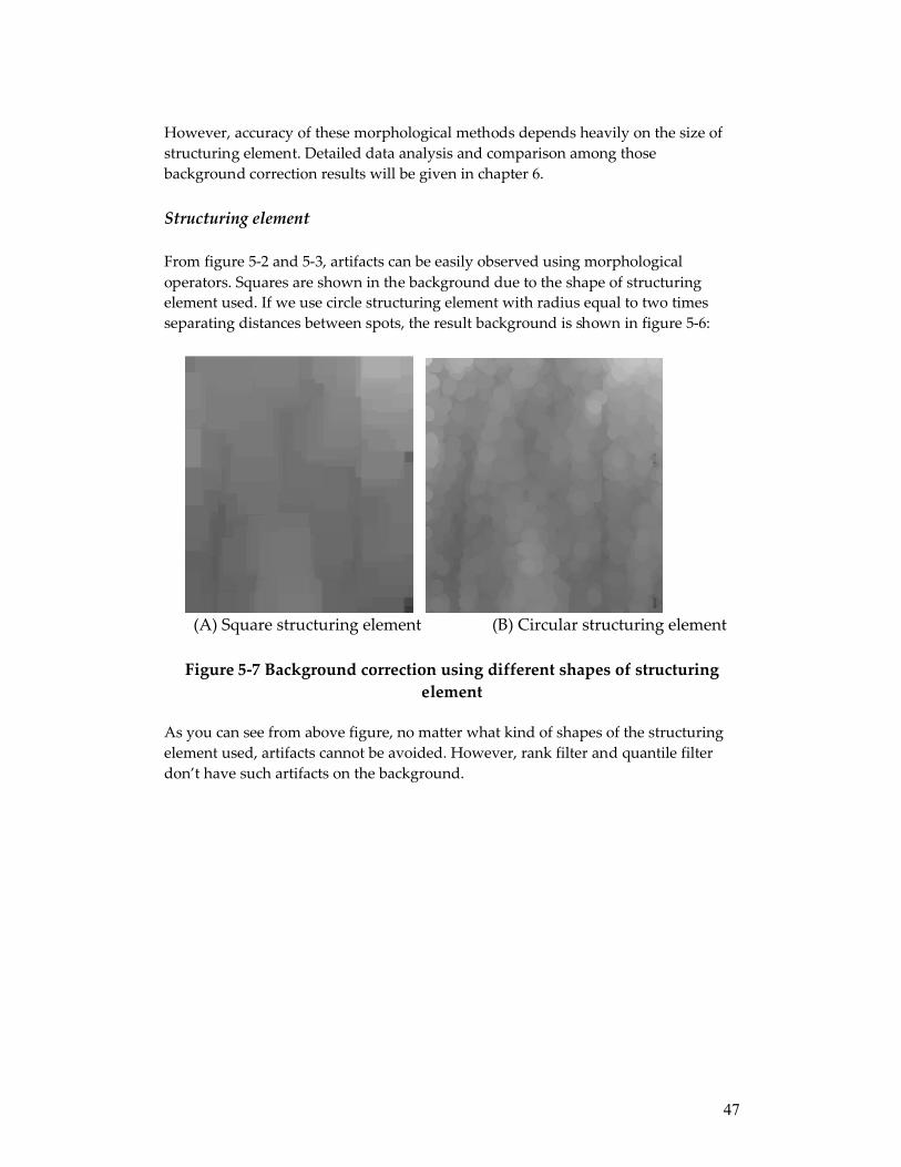
From figure 5-2 and 5-3, artifacts can be easily observed using morphological operators. Squares are shown in the background due to the shape of structuring element used. If we use circle structuring element with radius equal to two times separating distances between spots, the result background is shown in figure 5-6:
(A) Square structuring element (B) Circular structuring element
Figure 5-7 Background correction using different shapes of structuring element
As you can see from above figure, no matter what kind of shapes of the structuring element used, artifacts cannot be avoided. However, rank filter and quantile filter don’t have such artifacts on the background.

48
49
6.Data AnalysisIn this chapter, data obtained using various image processing methods will be analyzed. Performance between different background correction methods and overall performance between method used in this thesis and Genepix will be given in details.
Two Microarray images provided by Leiden University biology department have been investigated in this thesis, which use Zebrafish. These images, which were obtained, using different wavelength, have the same identical layout with 12x4 print-tip groups, each containing 19x19 spots, making total of 17328 spots per slide. The slides are replicates of each other such that the same gene is found at the same row and column.
6.1 Data PreprocessingUnderlying every microarray experiment is an experimental question that one would like to address. Finding useful and satisfactory answers relies on careful experiment design, optimal image processing and data retrieval method and the use of a variety of data-mining tools to explore the relationships between genes or reveal patterns of expression. Microarray data normalization and transformation becomes an indispensable task to make meaningful comparison of expression levels, and of transforming them to select genes for further analysis and data mining.
In this section, brief introduction will be given to Microarray data filtering and normalization.
6.1.1 Data transformation and filteringIn a spotted cDNA microarray experiment, a mixture of two cDNA samples that are differentially labeled with fluorescent dyes is hybridized to DNA sequences immobilized on a glass slide. Sequences from two targets hybridize to the complimentary probe sequences. The observed fluorescent signals at each spot are correlated with mRNA concentrations in the RNA samples from which cDNA targets were reverse-transcribed. The ratio of the two fluorescent signals at each spot is commonly used to infer the ratio of the mRNA concentrations in the two RNA samples. However, the ratio of the fluorescent signals is influenced by systematic effects from non-biological sources that can introduce biases and should be removed before calculating the relative levels of gene expression.
The process of removing such systematic effect is often referred to as normalization. Actually this process can further be divided into three steps: background correction, data transformation, and data normalization. Five background correction algorithms have been implemented, refer to chapter 5. Data transformation is applied to one microarray at a time to remove systematic effects from log-ratios. Normalization is the step to calibrate the signals from different channels and arrays to a comparable scale. A variety of data normalization

50
approaches have been proposed. Global normalization is implemented in this thesis and it will be discussed in the next section.
It has been demonstrated that the variance of log ratios also depends on signal intensity (Rocke and Durbin, 2001). When raw data are considered, variation increases when spot intensity increases. In this thesis, we applied log-transformation to the raw ratios of data from two channels. When log-transformation is applied toraw data, the variance is usually stable above certain intensity.
Before going in to detailed data analysis, data filtering is performed in order to remove unwanted or misleading signals in retrieved data set, which can affect the accuracy of the result.
In total, there are mainly three kinds of bad signals, and they are:• Spot with very high foreground intensity values or negative foreground
intensity values without background correction. These bad signals are mainly caused by noise such as electronic noise. Although many studies have offered insight on noise reduction in DNA microarrays, there are still certain kinds of noise, which can not be removed completely. In the image we used, there is no spot with negative foreground intensity and 440 spots with foreground intensity values higher than 10000, among 17328 spots on the red channel image.
• Spot with background intensities exceeding foreground intensities. This is caused by different background correction methods. Comparison between different background correction methods in terms of negative spot signals is given in section 6.3.
• Absent spots. The spot is too weak to be detected by certain segmentation methods. Thus spot signal is missing. It can be improved through segmentation methods we chose. There are only 152 spots missing among 17328 spots on the red channel image by watershed segmentation used in the implementation.
The signals with features introduced above should be removed from the data set before further analysis.
6.1.2 Data NormalizationThere are many sources of systematic variation in microarray experiments, which affect gene expression levels. Normalization is the process of removing such variation, e.g. for differences in labeling efficiency between two fluorescent dyes. In this case, a constant adjustment is commonly used to force the distribution of the log-ratios to have a median of zero for each slide [32]. The purpose of normalization is to balance the fluorescence intensities of the two dyes (green Cy3 and red Cy5 dye) as well as to allow the comparison of expression levels across experiments. Global normalization of log-ratios is used in the implementation.

51
Write R and G for the background corrected red and green intensities for each spot. Normalization is usually applied to the log-ratios of expression, which will be written GRM 22 loglog −= . The log-intensity of each spot will be denoted by 2/)log(log 22 GRA += , a measure of the overall brightness of the spot (The letter M is a mnemonic for minus while A is a mnemonic for add)[33] .
Global normalization assumes that the red and green intensities are related by a constant factor. That is, GkR •= , and in practice, the center of the distribution of log-ratios is shifted to zero:
))/((log/log/log 222 GkRcGRGR •=−→ (6-1)
A common choice for the location parameter kc 2log= is the median or mean of the log-intensity ratios for a particular gene set.
Two MA plots are shown in Figure 6-1. Figure 6-1(A) shows MA plot without normalization and (B) is the MA plot after applying global normalization to M values. Black bold lines are trend lines for two MA plots. As you can observe from the figure, trend line of the MA plot without normalization shows curvature; however trend line of MA plot with global normalization is almost parallel to the x axis because normalization removes curvature. Another different between these two MA plots is that M values of second plot center around the x axis, which means that the center of the distribution of log-ratios is shifted to zero. Without normalization, the log-ratios center around 1 in Figure 6-1(A) indicating a bias towards the green channel (Cy3 dye). Furthermore, global normalization reduces the spread of the log-ratios.
Red Channel MA PLot without Normalization
R2 = 0,025
-8
-6
-4
-2
0
2
4
6
8
0 2 4 6 8 10 12 14 16
A
M
Red Channel Normalized MA Plot
R2 = 0,0005
-4
-3
-2
-1
0
1
2
3
4
0 2 4 6 8 10 12 14 16
A
M
(A) Without Normalization (B) Global Normalization
Figure 6-1 MA Plot showing different trend lines with or without normalization method

52
Global normalization methods are still the most widely used methods. However such global normalization approaches are not adequate in situations where dye biases can depend on spot overall intensity and location on the array (print-tip). In the Figure 6-1 (B), the correlation between M and A is 0.0005, which shows little dependence of M on spot intensity).
There are other normalization methods such as paired-slides normalization, multiple slide normalization etc, which can reduce the spread of log-ratios more efficiently, and thus reduce dye biases. For details, please refer to Yee Hwa Yang [32].
6.2 General Data analysis In this section, we will analyze the data obtained through methods, which were introduced in previous chapters.
Figure 6-2 shows boxplot of foreground intensities without background correction among first 12 subgrids in Cy5 dye slide. From the figure, you can see the foreground intensities distribution.
The box has lines at the lower quartile, median, and upper quartile values. The whiskers are dotted lines extending from each end of the box to show the extent of the rest of the data. Outliers, depicted by ‘+’ symbol are data with intensities beyond the ends of the whiskers. The bold line inside each box represents a robust estimate of the uncertainty about the medians for box-to-box comparison. As you can observe from the box plot as well, there are many spots whose intensity values are higher than 10000, which are caused by noise. The line inside each box represents a robust estimate of the uncertainty about the medians for block-to-block comparison.
As you can see from the figure 6-2, there are spots with much higher intensity than it should be. The scale of Y-axis is 104 in figure 6-2, and foreground intensity values for red channel range from 0 to 65238. This proves that the image is severely contaminated by some kind of noise, especially electronic noise that causes much brighter pixel intensity. Current noise reduction method is not powerful enough to get rid of such kind of noise. However, this will cause inaccurate data results in data analysis stage. So pixels with intensity values higher 10000 are considered as contaminated spots, which can’t be recovered and thus are discarded.
In Figure 6-3, spots with very high foreground intensities are filtered out and you can take a close look at different foreground intensities distribution among 12 blocks.

53
Figure 6-2 Red channel boxplot of foreground intensities among first 12 Blocks
Figure 6-3 Red channel boxplot of foreground intensities among first 12 Blocks
Figure 6-4 shows the red and green channel foreground intensity distributions for whole image. From the figure, the robust estimate-line inside notch of red channel images is higher than that of green channel. Two lines inside notches are both centered on the box, which means no skewness occurring in both channels images.

54
Figure 6-4 Red and Green Channel Foreground Intensity Distribution of Whole Image
Figure 6-5 Circularity Histogram
Circularity of spot is very complicated to calculate in this case because there is no accurate way to get perimeter and area of the spot except in the way that number of pixels in segmented foreground is used as area and number of pixels in the segmented boundary pixels is denoted by perimeter. However, it is not accurate enough to measure the perimeter and area in such a manner, which ignores the actual length in terms of measurement unit for each pixels of interest. In order to calculate the length of perimeter, we have to know the angle between two adjacent pixels as depicted in Figure 6-5, and thus Length L1 can be know according to angle between these two adjacent pixels. This is very computational intensive.
In this thesis, two ways of circularity calculation are used. They are:1) Method 1: Number of pixels in foreground after segmentation is used as area
and number of pixels in boundary after segmentation is used as perimeter.

55
2) Method 2: Variance of the distance of each boundary pixels to the centroid of the spot.
In Figure 6-6 (A), circularity histogram using first calculation method is depicted. Circularity of most spots ranges from 0.5 to 0.9.Circle has highest circularity, which is 1. There are 197 spots among 17328 spots with circularity less than 0.5. This test result shows that watershed segmentation implemented in this thesis yield good result in terms of circularity of the spots. However, due to inaccurate way of circularity calculation, there are several spots with circularity higher than one. This should not happen because circle has the highest circularity value, which is 1. It is hard to explain in this way what it means by circularity higher than the circle.
(A) Method 1 (B) Method2Figure 6-6 Circularity Distribution
Figure 6-6 (B) shows the circularity histogram using second method. Distance of each boundary pixel to the centroid of the spot is calculated and variance of the distance is used as circularity estimate based on metric above ranging from 0 to 100. Circle has the highest circularity 100. From Figure 6-6 (A) and (B), the shape of the circularity histogram is very similar.
Correlation between different estimates
Commonly, when the signal level increases, the variance increases proportionally. A direct consequence of this is that the variance of the background will not be constant but will follow the spatial trend. This is demonstrated in Figure 6-7, where the standard deviation of the background pixels is plotted against the background intensity.

56
Figure 6-7 Correlation between Standard deviation and its background estimates using Quantile filter for red channel
The estimated background is highly correlated with the weakest spots, which have low foreground intensity value, see Figure 6-8. X-axis is Foreground intensity value and Y-axis is background intensity in the Figure 6-8. Correlation factor for red channel is 0968.02 =R and 1704.02 =R for green channel.

57
(A) Red Channel (B) Green ChannelFigure 6-8 Correlation between Foreground Intensity and Background
Intensity using Quantile Filter
F 635 Median-B635 vs Log-ratios
R2 = 0.2276-3
-2
-1
0
1
2
3
4
5
0 2000 4000 6000 8000 10000 12000
F 635 Median-B635
Log-r
atios
(A) Original Log-ratios (B) Normalized Log-ratios
Figure 6-9 Correlation between Log-ratios and corrected foreground intensity
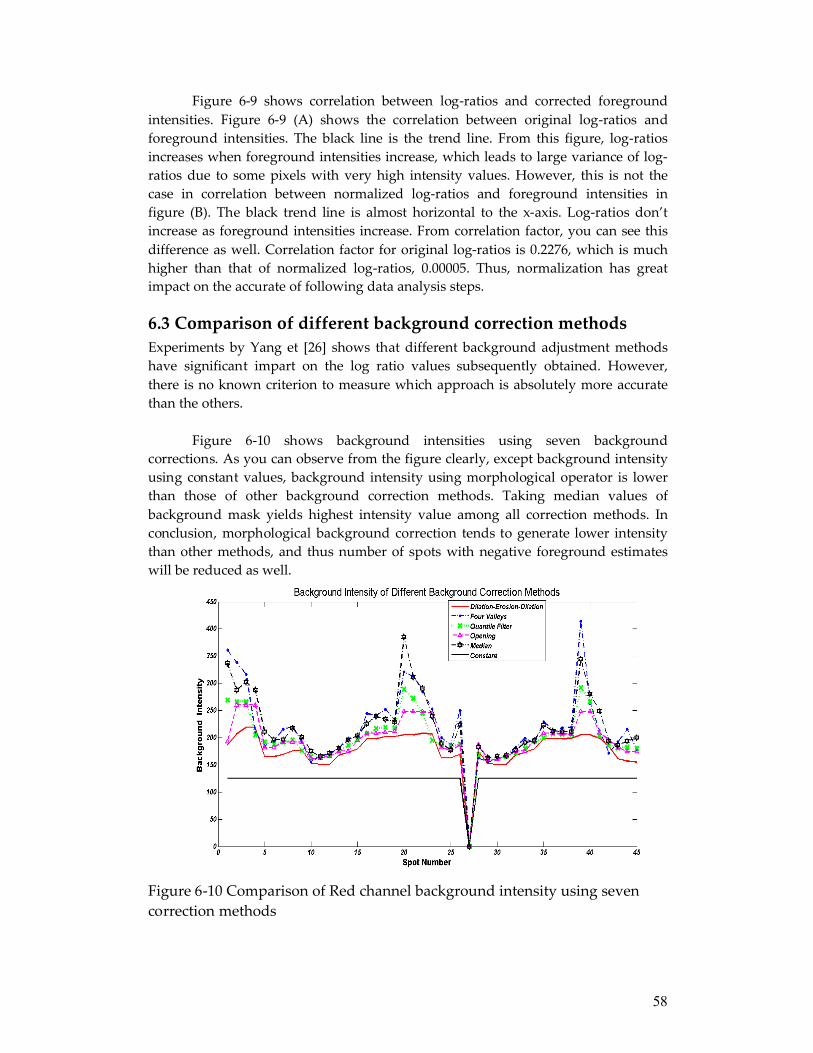
58
Figure 6-9 shows correlation between log-ratios and corrected foreground intensities. Figure 6-9 (A) shows the correlation between original log-ratios and foreground intensities. The black line is the trend line. From this figure, log-ratios increases when foreground intensities increase, which leads to large variance of log-ratios due to some pixels with very high intensity values. However, this is not the case in correlation between normalized log-ratios and foreground intensities in figure (B). The black trend line is almost horizontal to the x-axis. Log-ratios don’t increase as foreground intensities increase. From correlation factor, you can see this difference as well. Correlation factor for original log-ratios is 0.2276, which is much higher than that of normalized log-ratios, 0.00005. Thus, normalization has great impact on the accurate of following data analysis steps.
6.3 Comparison of different background correction methods Experiments by Yang et [26] shows that different background adjustment methods have significant impart on the log ratio values subsequently obtained. However, there is no known criterion to measure which approach is absolutely more accurate than the others.
Figure 6-10 shows background intensities using seven background corrections. As you can observe from the figure clearly, except background intensity using constant values, background intensity using morphological operator is lower than those of other background correction methods. Taking median values of background mask yields highest intensity value among all correction methods. In conclusion, morphological background correction tends to generate lower intensity than other methods, and thus number of spots with negative foreground estimates will be reduced as well.
Figure 6-10 Comparison of Red channel background intensity using seven correction methods

59
Let’s see the standard deviation of background intensity values using those seven background correction methods.
Figure 6-11 Comparison of Red Channel Background Standard Deviation using Seven Correction Methods
From figure 6-11, median values of background mask as background estimates and median values of four valleys yield highest standard deviation of background intensity. However, background correction methods using morphological operator have lower standard deviation. This figure shows that morphological background correction methods have smaller variability of background estimates.
From table 6-1, mean standard deviation of background estimates using different correction methods is calculated. Median and Four valley correction methods produce much higher approximately 100 times than morphological filter.
Methods Median Four valley
Opening Dilation Quantile
Mean SD 261.0588 135.0321 3.3627 2.6779 3.7687Table 6-1 Mean standard deviation of background estimates using different methods
Negative background corrected spots
There are four background estimates in red channel and one background estimate in green channel that exceed the foreground estimates using Quantile Filter, which is quite reasonable. Constant background correction method uses 5% of the pixels intensity within each block as background estimates and this method has only one negative background corrected spot, which means the percentile we chose in this thesis might be a little bit lower.

60
In conclusion, from Table 6-2, the number of negative background corrected spots is less than expected considering the biological layout of the experiment. Cross hybridization and other unspecific binding of RNA to the spots may add to the signals [31]. However, four valleys and Median background Correction methods have more number of negative background corrected spots among 17328 spots.
Background Correction Methods Number of negative corrected spots
Red 1Constant
Green 0Red 49Four valleys
Green 23Red 34Median
Green 23Red 0Dilation-Erosion-
Dilation Green 0
Red 1Opening Filter
Green 1Red 4Quantile Filter
Green 1
Table 6-2 Negative background corrected spots using different background correction methods
This data from Table 6-2 shows that not only they have less variability than other methods, but also morphological filter generate lower background estimates, which can reduce the number of negative background, corrected spots.

61
7. Conclusion and future workThis study is motivated by the development of a Microarray experiment analysis tool. Existing tools such as SPOT, GENEPIX, QUANTARRAY, aimed at supporting all the stages of a microarray experiment from image processing to data analysis. These tools include various gridding, segmentation and data extraction/analysis methods. However, there are still some issues, which need to find a better solution in order to achieve more accurate data without too much human intervention. For example, Genepix tool can’t deal with noisy image efficiently in gridding stage, and it requires user to adjust manually the gridding lines. This study focuses on seeking an automatic microarray image quantification method while data quality is still guaranteed.
We present a new automatic gridding method based on the Fourier transformation without human intervention. Usually, existing software tools require frequent human intervention to get accurate result. In this thesis, the gridding method is fully automatic on the eight test images. The advantage of this gridding algorithm among others is that it leaves much space for the choice of some critical parameters while accuracy of the subgrid finding result is still guaranteed. However, we use different methods to find spot lines, which, unlike finding the subgrids, turn out to require user intervention on some highly contaminated blocks. The biggest drawback of all the universal gridding algorithms is that either they require user adjustment, which cost effort or they don’t give enough freedom to choose some of the critical parameters, which have great impact on the gridding result. Both are important factors to be focused on future work.
However, to design such a method is time consuming. This step is critical for the following data extraction and data analysis steps. Thus a better solution than using image processing method to obtain grid and spot lines might be put into practice. Something can be done in the arrayer or print-tip before it is used to form a microarray image. For example, grids and spots lines can be dyed with special fluorescence dye in order to distinguish them from different genes of the DNA, which will be put on the arrayer. By doing this, it saves cost in the gridding step and thus more time can be saved for other important microarray image analysis steps.
In the segmentation phase, we examined the watershed segmentation technique. We did obtain satisfactory results with our proposed method. However, the choice of seed is critical and can lead to very different segmentation results. Future improvement of the choice of the seed is needed. The best seed choice is target dependent. Furthermore, tradeoff between computation complexity and choice of input image to the segmentation step is also important. If we use two images as input images to obtain masks, the computation cost is too high. Thus we use one image as input. A transformation could be applied to the original image so that segmentation will not include foreground pixels into background pixels and vice versa. Several experiments of transforming original images are performed, such as taking the highest intensity values between two images from red and green channel

62
to form the image as input to the segmentation step. We choose the method, which is introduced by Yang [26] because we compared different ways of forming a segmentation method and Yang’s method is the optimal one in terms of accuracy and computational complexity.
The motivation behind background adjustment is the belief that a spot’s measured intensity includes a contribution not specifically due to the hybridization of the target to the probe, but to something else, for example, non-specific hybridization and other chemicals on the glass. In this thesis, we implemented six background correction methods and comparison among those methods is performed. Our comparison of different methods for estimating such undesired contribution suggests that morphological operators provides a better estimate of background than other methods in terms of variability of background estimates and the number of negative corrected background spots. One of the main findings of our study is that the choice of background correction method has a larger impact on the log-intensity ratios than the segmentation method. Thus, finding the best segmentation method was not the primary focus of the paper.

63
Bibliography [1] D.Fenstemacher, Introduction to bioinformatics, Journal of the American Society for Information Science and Technology,vol.65,no.5,pp.440-456,2005
[2] A.B.Goryachev, P.F.MacGregor, and A.M.Edwards, Unfolding of Microarray Data, Journal of computational Biology,vol.8,no.443-461,2001
[3] Roberto Hirata,Junior Barrera,ROnaldo F.Hashimoto,DanielO.Dantas, Microarray Gridding by Mathematical Morphology, Computer Graphics and Image Processing, 2001 Proceedings of XIV Brazilian Symposium on Volume , Issue , Oct 2001 Page(s): 112 - 119
[4] J.Buhler,T.Ideker,and D.Haynor. Dapple: Improved Techniques forFinding Spots on DNA Microarrays. Technical Report UWTR 2000-08-05, University of Washington, 2000.
[5] A.Jain,T.Tokuyasu,A.Snijderts,R.Segraves,D.Albertson,and D.Pinkel.Fully Automatic Quantification of Microarray Image Data. Genome Res.,12(2):325-332,2003.
[6] R.Adams and L.Bischof. Seeded region growing. IEEETransaction on Pattern Analysis and machine Intelligence, 16:641-647, 1994.
[7] J.Angulo and J.Serra. Automatic analysis of DNA microarray images using mathematical morphology, Bioinformatics, vol.19,no.5,pp.553-562,2003.
[8] M.Schena. Microarray Analysis. John Wiley \& Sons, 2002
[9] Demin Wang, A Multiscale Gradient Algorithm For Image Segmentation Using Watersheds, pattern recognition,Vol 30, No. 12.pp. 2-43-2052, 1997
[10] Chang-Boem Park, Kwang-Woo Lee and Seong-Whan Lee, Automatic Microarray Image Segmentation Based on Watershed Transformation, Proceedings of the 17th international conference on Pattern recognition(ICPR’04)
[11] Li Qin, Luis Rueda, Adnan Ali and Alioune Ngon, Spot Detection and Image Segmentatin in DNA Microarray Data, Appl Bioinformatics. 2005;4(1):1-11.
[12] Hong Shan Neoh, Asher hazanchuk, Adaptive Edge Detection for Real-Time Video Processing using FPGAs, Global Signal Processing, 2004.

64
[13] Michele Ceccarelli, Giuliano Antoniol, A deformable grid matching approach for Microarray images, Image Processing, IEEE Transactions onVolume 15, Issue 10, Oct. 2006 Page(s): 3178 – 3188.
[14] G.Antoniol, M.Ceccarelli, A.Petrosino, Microarray Image Addressing based on the Randon transformation, Image Processing, 2005. ICIP 2005. IEEE International Conference on Volume 1, Issue , 11-14 Sept. 2005 Page(s): I - 13-16.
[15] Stefano Lonardi, Yu Luo, “Gridding and Compression of Microarray Images”, Computational Systems Bioinformatics Conference, 2004. CSB 2004. Proceedings. 2004 IEEE Volume , Issue , 16-19 Aug. 2004 Page(s): 122 – 130.
[16] Guiliano Antonio, Michele Ceccarelli, A Markov Radom Field Approach to Microarray Image Gridding, Pattern Recognition, 2004. ICPR 2004.Proceedings of the 17th International Conference on Volume 3, Issue , 23-26 Aug. 2004 Page(s): 550 - 553 Vol.3.
[17] Peter Bajcsy, An overview of DNA Microarray Grid Alignment and Foreground Separation Approaches, EURASIP journal on Applied Signal Processing, Volume 2006, Article ID 80163, Pages 1-13.
[18] Yoganand Balagurunathan, Naisyin Wang, Edward R. Fougherty, Danh Nguyen, Yidong Chen, Michael L.Bittner, Jeffrey Trent, Raymond Carrol, “Noise factor analysis for cDNA microarrays,” Journal of Biomedical Optics.
[19] J.Han and M.Kamber, Data mining: Concepts and Techniques, Morgan Kaufmann, San Francisco, Calif, USA, 2001.
[20] L.Vincent and P.Soille, Watersheds in digital spaces: An efficient algorithm based on immersion simulations, IEEE Trans. Pattern Analysis Mach. Intell. 13,583-598(1991)
[21] J.Serra, Image analysis and Mathematical Morphology. Academic Press, London (1982).
[22] S.Beucher, The watershed transformation applied to image segmentation, 1999
[23] Eisen, M.B.(1999). ScanAlyze User manual. Stanford University, Palo Alto. http://rana.lbl.gov.
[24] Axon Instruments, Inc. GenePix 4000A User’s Guide, 1999.

65
[25] GSI Lumonics. QuantArray Analysis Software, Operator’s Manual, 1999.
[26] Yang, Y.H., Buckley, M.J., Dudoit, S., and Speed, T.P.(2002). Comparison of methods for image analysis on cDNA Microarray data. Journal of Computational and Graphical Statistics 11. 108-136.
[27] Buckley, M.J.(2000). Spot User’s Guide. CSIRO Mathematical and Information Sciences, Sydney, Australia. http://www.cmis.csiro.au/iap/Spot/spotmanual.htm
[28] Anders bengtsson, Henrik Bengtsson, Microarray image analysis: background estimation using quantile morphological filters. BioMed Central Ltd, Feb, 2006.
[29] Soille, P.(1999),Morphological Image Analysis: Principles and Applications,Springer-Verlag Berlin Heidelberg.
[30] Anders Bengtsson. Microarray Image Analysis: Background Estimation using Region and Filtering Techniques. Master’s thesis, Lund University E40, December 9,2003.
[31] Kooperberg C, Fazzio T, Delrow J, Tsukiyama T:Improved Background Correction for Spotted DNA Microarrays. Journal of Computational Biology 2002.
[32] Yee Hwa Yang, Sandrine Dudoit, Percy Luu and Terence P.Speed, Normalization for cDNA Microarray Data, Nucleic Acids Research, 2002, Vol. 30, No. 4 e15 © 2002 Oxford University Press.
[33] Gordon K. Smyth and Terry Speed, Normalization of cDNA Microarray Data, April, 2003, Application to Neuroscience.

66
Acknowledgement
I would like to express my gratitude to all those who gave me the possibility to complete this thesis.
The majority of my thanks go to my supervisor Fons J.Verbeek whose help, stimulating suggestion and encouragement helped me in the completion of the thesis.
Second, my special thanks go to our secretary Maggie de Wert for her understanding and strong support during the most difficult time of my life.
Third, I would like to thank my classmates Tian Feng, Yan Gao nd Jinshuo Liu who gave me useful advice and supplied with detailed information for my thesis work.
Fourth, I would like to thank Yun Bei who is of great help in difficult times.
Finally, I would like to give my special thankfulness to all my family members, especially my younger brother and my beloved mother. Thank my brother for taking over my responsibilities such that I have time concentrating on the thesis. Last but the most important person who I want to thank is my mother. Without her support, Iwouldn’t have the chance to pursue my study in Netherlands.