Computers & Geosciences 40 (2012) 185–193

Contents lists available at ScienceDirect

Computers & Geosciences

0098-30

doi:10.1

n Corr

E-m

Eevaliis

journal homepage: www.elsevier.com/locate/cageo

MATLAB script for analyzing and visualizing scanline data

M. Markovaara-Koivisto a,n, E. Laine b

a Aalto University School of Science and Technology, P.O. Box 16200, FIN-00076 Aalto, Finlandb Geological Survey of Finland, Betonimiehenkuja 4, FIN-02151 Espoo, Finland

a r t i c l e i n f o

Article history:

Received 13 January 2011

Received in revised form

12 July 2011

Accepted 13 July 2011Available online 29 July 2011

Keywords:

Visualization

Clustering

Discontinuity

2D

3D

Computer code

04/$ - see front matter & 2011 Elsevier Ltd. A

016/j.cageo.2011.07.010

esponding author. Tel.: þ358 9 470 22734; fa

ail addresses: Mira.Markovaara-Koivisto@tkk.

a.Laine@gsf.fi (E. Laine).

a b s t r a c t

Scanline surveys consist of directional and qualitative measurements of rock discontinuities. These

surveys are used in geologic and engineering investigations of fractured rock masses. This paper

introduces a new MATLAB script developed for visualizing results from scanline surveys as traces in 2D

and disks in 3D. The script is also able to cluster orientation data and to present statistical summaries

and to reflect the change in degree of rock brokenness along the scanline. Advantages of this new

script are that it can present undulating discontinuities as wavy surfaces and different discontinuity

properties using color codes. An intensity rose diagram is utilized to visualize interdependency of

certain properties and orientation. This new script has a potential for preprocessing vast amounts of

scanline and oriented drill core logging data before using it in 3D discontinuity network modeling. The

script is demonstrated using data concerning rock fracturing gathered from a dimension stone quarry in

Southern Finland.

& 2011 Elsevier Ltd. All rights reserved.

1. Introduction

Discontinuity surveys are a fundamental component of rockquality estimation, hydrological modeling, and many other fieldsin rock engineering (Wu et al., 1999; Grenon and Hadjigeorgiou,2003a; Black, 1994). In 1978 the International Society of RockMechanics (ISRM) specified scanline survey as an objectivemethod for recording and describing rock fracturing on an out-crop, meaning that the results of a scanline survey are relativelyobjective. In contrast, describing only the discontinuities whichseem to be important can be considered as a subjective methodof surveying the fracturing. The scanline logging method isdescribed in detail by Priest and Hudson (1981) and ISRM (1978).

Statistical estimation of the discontinuity network at depthwithin the rock mass relies on observations made on the surfaceand drill holes. Observations made on the rock wall are morecomprehensive, because the dimensions of the discontinuities arebetter recorded. A scanline method, for collecting such data, hasbeen recommended by Grenon and Hadjigeorgiou (2003b).

The scanline survey method is common in gathering informa-tion for the discrete element method (DEM) to model deformationprocesses and for a discrete fracture network (DFN) to modelhydraulic behavior of fractured media (Chesnaux et al., 2009).Results of a scanline survey can be visualized in 2D and 3D using

ll rights reserved.

x: þ358 9 470 22731.

fi (M. Markovaara-Koivisto),

softwares developed for the above applications. One softwaredeveloped purely for visualizing rock mass is linear isometricprojection of rock mass (LIP-RM, Turanboy and Ulker, 2008),which simulates the discontinuities as planar and persistentsurfaces inside the domain. PETREL software (Schlumberger;PETREL, 2007) can be used for visualizing the discontinuities asequal sized disks along the measuring line and for analyzing thediscontinuity sets for subsequent DFN modeling utilizing Golderalgorithms (Golder Associates) as presented by Chesnaux et al.(2009). Scanline survey is also used to gather initial data formodeling stone blocks in optimizing dimension stone quarrying.3D-BlockExpert software (Mosch et al., 2010) builds blocks usinginformation from three orthogonal scanlines. Discontinuitiesare considered as persistent planes. These published softwareshave two common deficiencies: describing the discontinuities asstraight planes, and extending the simulated discontinuitiesthroughout the model, although they are important factors indefining rock mass quality. Even Turanboy and Ulker (2008)criticized these aspects of the LIP-RM software they developed.FracMan (Golder Associates) discontinuity DFN simulation soft-ware takes into account also discontinuity size distribution(Zhang and Einstein, 2000). As the visualization and analysis ofthe scanline data are drawn to DEM and DFN discontinuitynetwork modeling, many of the surface properties (for instance,roughness and undulation) are not utilized in the visualizations.

In the present paper the aim was to develop a MATLAB scriptto visualize and analyze scanline measurements, which takes intoaccount also undulation and trace lengths of the discontinuities.The undulating discontinuities are presented as wavy and the

Fig. 2-2. Discontinuities’ apparent dip can be used for 2D visualization of tight

discontinuities, whose orientation cannot be measured otherwise. Trace lengths

above and below the scanline are important parameters of discontinuity visuali-

zation, and are used to calculate the midpoint of the trace.

M. Markovaara-Koivisto, E. Laine / Computers & Geosciences 40 (2012) 185–193186

straight discontinuities as planar spheres or disks. In this work,visualization aspects were emphasized; discontinuities in 3Dvisualizations are color coded to indicate their properties suchas roughness or discontinuity set. In stereographic projection thesets are distinguished with the same color codes to enhanceconsistency of the visualizations. In addition, the intensity rosediagram (M MA, 2009) shows frequency of discontinuities’ prop-erties in the orientations.

The developed MATLAB tools, Visual_Scanline2D and Visual_Scan-line3D, need only the standard MATLAB (a registered trademark ofThe Mathworks Inc.) functions. The 2D visualization can be used toreproduce a rock wall scene of the discontinuity traces intersectingthe scanline.

The new analyzing and visualizing tools were put into a testwith scanline data from a dimension stone quarry at Mantsala,Southern Finland. The quarry was chosen because of easy acces-sibility to several excavation levels that have rock walls in twonearly orthogonal orientations. The rock type at the area ismigmatitic granodiorite with granitic neosomes consisting about35% of the rock, and sparse amphibolite veins, which follow thegeneral foliation, dipping to the east at 22 degrees. The studieddiscontinuities were easily visualized and broken areas located. Inaddition, the orientation of the main discontinuity sets anddiscontinuity densities within were printed out, and preferredorientations for the discontinuity properties were easily illu-strated on rose diagrams.

Fig. 2-3. Using the orientation data of a scanline and a discontinuity, the

intersection of a discontinuity and the rock wall can be calculated for the 2D

scanline drawing. A discontinuity trace on a rock wall is seen as the dashed line on

the drawing.

2. Scanline survey

Scanline logging is a technique in which a line is drawn overan outcropped rock surface and all the discontinuities intersectingit are measured and described (Priest and Hudson, 1981)(Fig. 2-1). As the parameters of the discontinuities are measured,described and statistically analyzed, the degree of brokenness orintactness of the bedrock may be estimated.

Scanline logging results are usually presented as a 2D drawingof the scanline and the discontinuities intersecting it (Milnes andGee, 1992; Ortega et al., 2006) or more as a drawing of the wholerock face or outcrop (Priest, 2004).

To produce a 2D or 3D visualization of the fracturing, thefollowing data are needed: length and orientation of the scanline,the starting and ending points of the scanline as measured withGPS, reading of measuring tape at a crosscut of the scanline and adiscontinuity, orientation of the discontinuities, trace lengthsabove and below the scanline, wave length and amplitude ofundulating discontinuities, and apparent dips for discontinuitieswhich orientations cannot be otherwise measured. Fig. 2-2 showshow apparent dip and trace lengths are measured. The midpointof the trace is calculated trigonometrically.

When orientations of a scanline and the intersecting disconti-nuity are known, the apparent dip, used in the 2D line drawing,can be calculated trigonometrically. See Fig. 2-3, where b isdiscontinuity’s dip, r scanline’s trend, and a apparent dip.

Some discontinuities might be nearly parallel to the mappingsurface, or even comprise parts of the surface. In a line drawingthese discontinuities are not presented in a realistic way. A betterway to illustrate them is a 3D model.

Fig. 2-1. A view from above of a horizontal scanline on an outcropped rock wall.

Scanline measuring tape is a straight line, which touches the outcrop only at its

protruding parts. The real intersection of the scanline and a discontinuity in an

irregular rock wall must be projected to the measuring tape (dashed lines).

3D visualization of discontinuities is based on informationgathered from a rock surface and contains some unknowns. Somegeneralizations therefore must be made. The discontinuities arevisualized as thin round disks, as the actual shapes of the disconti-nuities are not known. This practice is widely used because of thedisks’ simple parametric description (for example, Zhang andEinstein, 2000). Furthermore, the maximum length of the disconti-nuities and their real middle points are unknown. Because the tracelengths measured on the rock walls are the discontinuities’ longestobservable dimension, these are used as the diameter of the disks,and the disks middle points are presumed to lie on the rock wall. Itshould be noted that measured trace lengths are biased dueto relative orientation of the discontinuities and the scanline.In addition they are biased due to discontinuities size, as largerdiscontinuities are more likely to be sampled on a scanline thansmaller ones, and the smallest discontinuities are truncated and thediscontinuities extending beyond the rock wall are censored (Zhangand Einstein, 2000). These errors should be corrected before usingthe data in any DFN simulations.

2.1. Overview of scanline data and input data

Gathered information includes the following properties in thefollowing order: distance from the starting point (m), apparentdip (1), trace length above the scanline (m), trace length below thescanline (m), dip (1), dip direction (1), wave length (m), amplitude(m), straightness (1¼straight, 2¼undulating, 3¼curvy), rough-ness (1¼smooth, 2¼slightly rough, 3¼rough), discontinuitytype (1¼open, 2¼closed, 3¼filled, 4¼slickenside, 5¼dyke), endingtype (1¼through going, 2¼both ends visible, 3¼one end visible,

M. Markovaara-Koivisto, E. Laine / Computers & Geosciences 40 (2012) 185–193 187

4¼neither end visible), aperture (mm), possible mineral 1, mineral2, and mineral 3 (codes from 1 to n) on discontinuity surface.

Aperture and codes allocated to different classes of straight-ness, discontinuity type, ending type, roughness, and possiblediscontinuity filling minerals may be used to classify and colorcode the disks in the 3D visualization. Also any other predefinedproperties may be used as a basis for the classification. Otherproperties are used for generating the drawings and in statisticalanalysis.

2.2. 2D and 3D objects

Large scale roughness or undulation of discontinuity surfacesplays an important role in defining surface friction parameter Jr

in the Q-system (Barton et al., 1974). Undulation can easily beshown in the illustrations, if its parameters (wave length andamplitude) are measured during scanline mapping.

The lines representing the discontinuities in the 2D visualiza-tion were created between the calculated end points of disconti-nuities. The curves representing the wavy discontinuities werecreated as sine curves along the trace length using the same wavelength and amplitude measured in the field using the followingequation:

Y ¼ amplitudensinððtracelength=wavelengthn2pÞ: ð1Þ

The curves were then moved to their real locations according tothe calculated middle points of the discontinuities and rotated tothe orientation observed in the field.

In the 3D visualization the straight discontinuities were pre-sented as disks which have a diameter equal to the measuredtrace length and orientation as observed in the field. Disks aredrawn using 128 equally spaced points to represent their edges.To create the wavy surfaces, a square shaped grid was used. Tracelength was used as the size of the grid, and the z dimension wascalculated using Eq. (1). Points further away from the center pointof the discontinuity were deleted from the grid leaving a sphericalgrid remaining. An illustration of the method is shown in Fig. 2-4.The grid was moved to the calculated center point of thediscontinuity and rotated to the measured orientation. The usercan define the density of the grid and can therefore influence thecomputing time and the resolution of the illustration. Recom-mended resolution for the first computation with a new data setis 0.1 m to secure a short calculation time.

2.3. 2D analysis

Numerical calculations concerning fragmentation of the rockmass along the scanline can be carried out based only on the

Fig. 2-4. Undulating surfaces were created as grids. (A) Cells outside the radius of the di

as a sine function of the amplitude and wave length of the discontinuity.

location of the intersections of the scanline and discontinuities. Theresults can be easily presented in 2D above the scanline as columnarbars. With this software the user may view the number ofdiscontinuities or Rock Quality Designation (RQD) (Deere, 1963).

2.4. Statistical tools for directional data

Statistics of the discontinuity analysis can be viewed from atree type MATLAB structure named RESULTS. Grouping of dis-continuities into discontinuity sets and characterization of theirorientations are important parts of rock engineering. The struc-ture therefore contains information about the scanline and thediscontinuity sets.

Information about the scanline contains properties such aslength, dip, and dip direction, and x, y, and z coordinates of scanline’sstarting point. Information given out concerning the discontinuitysets is their mean dip and dip direction, number of discontinuitieswithin the set, mean trace length and standard deviation, disconti-nuity spacing and density along the scanline, and orientationcorrected discontinuity spacing and density calculated perpendicu-lar to the mean orientation of the particular set.

The trace length and discontinuity spacing data need to becorrected due to some geometrical errors, censoring effect, andthe effect caused by the scanline length (La Pointe and Hudson,1985; Hofrichter and Winkler, 2006; Priest and Hudson, 1981;Sen and Kazi, 1984). Here only geometrical errors have beencorrected, because other corrections need a distribution analysisbefore correct processing can be applied.

Orientation dependency of discontinuity properties is visua-lized here with stacked rose diagrams. In addition to presentingthe number of discontinuities in a certain direction, the orienta-tion sectors are divided into smaller pieces representing thenumber of observations of properties such as trace length andsurface roughness.

2.4.1. The grouping method

Classification clustering of directional data is particularly used instructural geology and rock engineering. Various methods have beendeveloped, starting from Schmidt’s counting method on stereo-graphic plots (Schmidt, 1925). Later the kernel density estimationwas introduced (Priest, 1994; Duda and Hart, 2000), and a countingmethod which minimized an objective function (Shanley andMahtab, 1976) and uses optimization of a probability function ona sphere (Wallbrecher, 1978) was developed. The automated expertsupervised method was developed by Pecher (1989). Dershowitzet al. (1996) later developed the stochastic reassignment method to

scontinuity were deleted from the grid. (B) Z coordinate on the grid was calculated

Fig. 2-5. An example of grouped pole vectors on a unit sphere with dip 90 at the

top and 0 at the bottom.

M. Markovaara-Koivisto, E. Laine / Computers & Geosciences 40 (2012) 185–193188

partition vectors. Hammah and Curran (1998) used fuzzy logic andthe similarity measure to generate the clusters.

In Visual_Scanline3D, the Kmeans method is used to clusterdirectional data into user-defined number of groups around initialcenter points given by the user. One group is reserved for therandom discontinuities. Details of the method are given later. Theuser may correct clustering within a user interactive window. Thepossibility for the user to change the grouping is essential,because the data might be sparse and unrepresentative whichhinder automatic grouping. The user may also cluster the datawith other programs, and import the clustering results. Thedivision of discontinuities into different sets is utilized in visua-lizing the discontinuities with different colors and as a basis forstatistical analysis of the gathered data, and the related geome-trical corrections.

The K means method is a learning algorithm, in which thegiven K number of clusters competes to own their share of the N

data points in an I dimensional space, in which the dimensionsrepresent the discontinuity properties given. Each cluster has amean value, which the user gives at the beginning of the iteration,by pointing them from a stereographical projection of the dis-continuity data. The Kmeans algorithm calculates the distancebetween points and works iteratively in two steps. First the dataare grouped with the nearest means. Then the means arecalculated again for the groups. Then the steps are repeated untilthe assignments do not change. The method is explained in detailby MacKay (2003).

Here grouping was carried out on the pole vectors, which canbe calculated in a Cartesian coordinate system from dip and dipdirection of the discontinuity surface as follows:

y¼ cosðdipdirþ1801Þcosð901�dipÞ North direction,

x¼ sinðdipdirþ1801Þcosð901�dipÞ East direction,

z¼ sinð901�dipÞ Downward: ð2Þ

The Kmeans grouping method relies on distances betweenpoints. As the points are scattered on a sphere, arclength,recommended to be used as the distance measure by Kloseet al. (2005), was adopted. Arclength DS between the normalvectors of a discontinuity N and the center point of a cluster Ncluwas calculated along the unit sphere’s surface

DsðN,NcluÞ ¼ ðarccosðNUNcluÞÞ2, ð3Þ

where � is dot product of the two vectors.The results of the data grouping according to orientation

are visualized not only on a stereographic projection, but alsoon a spherical surface, on which dip is plotted on the verticalaxis ranging from 01 at the bottom of the sphere to 901 at thetop of the sphere. Fig. 2-5 presents an example. Azimuth isplotted on x and y axes in the usual manner. The advantageof this visualization compared to more common stereographicprojection or pole vectors on a lower hemisphere presentation isthat the data seem continuous in a 3D visualization as it is drawnaround a sphere, and different orientations are divided onto agreater surface.

The unit vector’s coordinates on this spherical surface arecalculated with the following formulas:

x¼ cosðarcsinðzÞÞnsinðdipdirþ180Þ

y¼ cosðarcsinðzÞÞncosðdipdirþ180Þ

z¼ ðdip�45Þ=45: ð4Þ

2.4.2. Mean orientation

The mean orientation of the discontinuities belonging to thesame discontinuity set were calculated as presented by Hammahand Curran (1998) from eigenvectors associated with the highest

eigenvalue of orientation cosine matrix of discontinuities inthe set.

First the orientation cosines were calculated with the follow-ing formulas:

x¼ cosð90�dipÞnsinðdipdir�180Þ

y¼ cosð90�dipÞncosðdipdir�180Þ, if dipdir4180 ð5Þ

x¼ cosð90�dipÞnsinðdipdirþ180Þ

y¼ cosð90�dipÞncosðdipdirþ180Þ, if dipdiro180

z¼�sinð90�dipÞ:

Then orientation cosine matrix was calculated using theformula

S¼

XN

j ¼ 1

xjxj

XN

j ¼ 1

xjyj

XN

j ¼ 1

xjzj

XN

j ¼ 1

xjyj

XN

j ¼ 1

yjyj

XN

j ¼ 1

yjzj

XN

j ¼ 1

xjzj

XN

j ¼ 1

yjzj

XN

j ¼ 1

zjzj

26666666666664

37777777777775

, ð6Þ

where N is number of discontinuities belonging to the same group.The orientation matrix was normalized with the number of

discontinuities in the set, and eigenvalues were calculated. Aneigenvector (xeig, yeig, zeig) associated with the highest eigenvaluewas calculated, and the mean orientation of the discontinuity setwas derived with the following formulas:

SetDip¼ 90�9arcsinðzeigÞ9 ð7Þ

SetDipDir¼ 9arctanðxeig=yeigÞ9, if xeig40 & yeig40

SetDipDir¼ 180�9arctanðxeig=yeigÞ9, if xeig 40 & yeigo0

SetDipDir¼ 180þ9arctanðxeig=yeigÞ9, if xeig o0 & yeigo0

SetDipDir¼ 360�9arctanðxeig=yeigÞ9, if xeig 40 & yeigo0:

2.4.3. Discontinuity spacing

Discontinuity spacing is calculated within each discontinuityset. The distance between the discontinuities in the same set canbe calculated from the data gathered in the scanline mapping

M. Markovaara-Koivisto, E. Laine / Computers & Geosciences 40 (2012) 185–193 189

using an orientation correction factor. The angle (C) between thescanline and the mean orientation of a discontinuity set iscalculated with the dot product of these vectors, and then thecorrection factor (CF) is calculated with the formula

CF ¼ 9cosðcÞ9: ð8Þ

The CF remains always above 0.2, as suggested by Hofrichterand Winkler (2006) to avoid exaggeration.

Interdiscontinuity distances are printed to the RESULTS struc-ture, and plotted as a box-and-whiskers diagram for each dis-continuity set. An inverse is taken from the mean distance toobtain the discontinuity density.

2.4.4. Trace length

All observed trace lengths are presented as a histogram. Foreach discontinuity set, trace lengths are plotted as a box-and-whiskers diagram, and average values and standard deviationsare calculated. In addition, trace lengths are divided into groupswith 1-m intervals, which are used for visualizing the preferentialorientation of trace lengths in an intensity rose diagram. Dis-continuities which have a shallower dip than 451 were excludedfrom the intensity rose diagram. This is because these disconti-nuities may belong to a nearly horizontal group, where the actualdip direction may change arbitrarily.

2.5. Presentation of the results

Together with the 2D visualization of the discontinuities,numerical information gathered along the scanline can be pre-sented above the scanline as columnar bars. Here the number ofdiscontinuities per meter and RQD values can be shown with ahalf meter interval as seen in Fig. 3-3.

In case only trends of discontinuities are measured, the resultscan be presented as polar histograms known as discontinuityrosettes. When trend and plunge are measured, the results canbe presented on a stereogram (La Pointe and Hudson, 1985).A stereographic projection is used to show relationships betweenthe major discontinuity planes (Khanlari and Mohammadi, 2005).

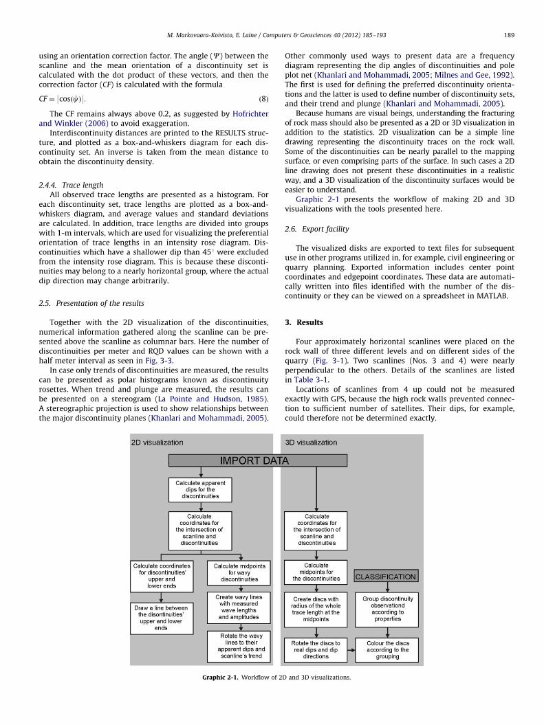
Graphic 2-1. Workflow of 2D

Other commonly used ways to present data are a frequencydiagram representing the dip angles of discontinuities and poleplot net (Khanlari and Mohammadi, 2005; Milnes and Gee, 1992).The first is used for defining the preferred discontinuity orienta-tions and the latter is used to define number of discontinuity sets,and their trend and plunge (Khanlari and Mohammadi, 2005).

Because humans are visual beings, understanding the fracturingof rock mass should also be presented as a 2D or 3D visualization inaddition to the statistics. 2D visualization can be a simple linedrawing representing the discontinuity traces on the rock wall.Some of the discontinuities can be nearly parallel to the mappingsurface, or even comprising parts of the surface. In such cases a 2Dline drawing does not present these discontinuities in a realisticway, and a 3D visualization of the discontinuity surfaces would beeasier to understand.

Graphic 2-1 presents the workflow of making 2D and 3Dvisualizations with the tools presented here.

2.6. Export facility

The visualized disks are exported to text files for subsequentuse in other programs utilized in, for example, civil engineering orquarry planning. Exported information includes center pointcoordinates and edgepoint coordinates. These data are automati-cally written into files identified with the number of the dis-continuity or they can be viewed on a spreadsheet in MATLAB.

3. Results

Four approximately horizontal scanlines were placed on therock wall of three different levels and on different sides of thequarry (Fig. 3-1). Two scanlines (Nos. 3 and 4) were nearlyperpendicular to the others. Details of the scanlines are listedin Table 3-1.

Locations of scanlines from 4 up could not be measuredexactly with GPS, because the high rock walls prevented connec-tion to sufficient number of satellites. Their dips, for example,could therefore not be determined exactly.

and 3D visualizations.

Fig. 3-1. Scanlines on the rock faces (A) on the southern wall and (B) on the northern wall of the Mantsala dimension stone quarry.

Table 3-1Details of the scanlines at the Mantsala quarry case study.

Trend (deg.) Plunge (deg.) Length (m) Number of

discontinuities

Scanline 1 230 Rising (þ)4.4 33 62

Scanline 2 238 Descending (�)1.6 23 61

Scanline 3 328 Descending (�)1.7 15 44

Scanline 4 333 Horizontal 0.0 20 57

Fig. 3-2. 2D drawing of the discontinuities intersecting Scanline 4. The gray sheet illustrates the rock wall, and the thick dashed line the scanline.

M. Markovaara-Koivisto, E. Laine / Computers & Geosciences 40 (2012) 185–193190

The reader may test the 2D and 3D visualization scripts withTestdata.txt, which is the data from Scanline 4. Contents of theTestdata.txt are as listed in Section 2.1.

3.1. 2D visualization and analysis

The discontinuities intersecting the scanlines were visualizedfirst in 2D as line drawings (Fig. 3-2). Undulating discontinuitiesare presented as wavy lines, the geometries of which are based onthe field observations. Instructions for making similar visualiza-tions can be found in Manual.txt.

In Fig. 3-3 a bar diagram showing the number of disconti-nuities cross cutting the scanline is drawn above the scanlinewith a 0.5-m interval. The legend is automatically scaled to themaximum. A similar illustration is also made for RQD value.

3.2. Orientation analysis

The main discontinuity sets were defined by presenting theorientations measured in the scanline survey in a stereoplot.Fig. 3-4A presents an example of automatic clustering, in which

some of the random discontinuities (diamonds) were grouped intothe discontinuity set indicated with triangles. The results correctedby a hand-picking tool are presented in Fig. 3-4B; random disconti-nuities are within one group, poles also on opposite sides of thestereogram are taken into account, and discontinuities in the mainjoint sets are delimited to have 7101 fluctuations in dip directionand 7151 in dip.

Rose diagrams were drawn with DIPS by Rocscience to visualizethe strikes of discontinuities in the different scanlines (Fig. 3-5). Thisproperty is not included inVisual_Scanline3D functions. Scanline 3,which is perpendicular to Scanlines 1 and 2, presents a differentiat-ing rose diagram. Discontinuities parallel with Scanlines 1 and 2 arebetter represented in Scanline 3. In contrast, Scanlines 1 and 2 betterrepresent the discontinuities parallel to the wall on which Scanline3 was situated.

The rose diagram method was also used in Visual_Scanline3D forpresenting commonness of properties in the direction of differentstrikes. In Fig. 3-6 roughness of the discontinuity surfaces ispresented in the same scanlines as in Fig. 3-1A. It can be seen thatthe roughest surfaces are orientated in southeast–northwest, andthe smoothest orientated in a northeast–southwest direction. Only

Fig. 3-3. Number of discontinuities per meter is visualized above Scanline 4 as a bar diagram.

Fig. 3-4. Main discontinuity sets defined by stereoplots of the orientations of the discontinuities intersecting the Scanline 4. (A) Result of automatic Kmeans clustering

with user-defined centroids of the discontinuity sets. (B) User-corrected discontinuity sets.

Fig. 3-5. Rose diagrams depicting the preferential orientations of the discontinuities intersecting Scanlines 1, 2, and 3. Images are drawn using Dips by Rocscience.

M. Markovaara-Koivisto, E. Laine / Computers & Geosciences 40 (2012) 185–193 191

discontinuities where dip is greater than 451 are taken into accountin Fig. 3-6 to make it comparable with Fig. 3-5.

3.3. Statistical analysis

Statistical analysis within the discontinuity sets is carried outwith Visual_Scanline3D. Table 3-2 presents results of statisticalanalysis of Scanline 4, the Testdata.txt. Five discontinuity setswere found along Scanline 4. It seems like the three maindiscontinuity sets and the horizontal set have been utilized inthe quarry planning, because their orientations are parallel ornearly orthogonal to the quarry’s walls. Set 6 contains the randomdiscontinuities. This set’s orientation and orientation-corrected

discontinuity spacing and density are italicized, because they areunreliable due to orientation’s high variation within the group.

3.4. 3D visualization

This section will be presenting making the 3D visualizationswith Visual_Scanline3D. Undulating discontinuities are presentedas wavy surfaces, the geometries of which are based on the fieldobservations. Instructions for drawing similar visualizations canbe found in Manual.txt.

Fig. 3-7 represents a 3D drawing of the discontinuities inScanline 4. Color coding of the discontinuity sets is based on thedivision in Fig. 3-4. Similar visualizations can be drawn for other

Fig. 3-6. Intensity rose diagrams showing roughness in Scanline 1, 2, and 3.

Table 3-2Results of statistical analysis of Scanline 4.

Set 1 Set 2 Set 3 Set 4 Set 5 Set6 (random)

Dip (deg.) 76 83 77 77 26 74

Dip direction (deg.) 327 034 347 288 086 160

Number of discontinuities 13 9 8 5 2 18

Mean trace length (m) 1.96 2.31 1.50 1.22 1.66 1.37

Standard deviation 1.90 1.82 1.99 0.84 0.48 1.27

Discontinuity spacing (m) 1.62 1.91 1.18 3.08 0.67 1.00

Discontinuity normal spacing (m) 1.36 0.38 0.74 2.96 0.26 1.00

Discontinuity density (1/m) 0.62 0.52 0.85 0.32 1.49 0.71

Discontinuity normal density (1/m) 0.74 2.62 1.36 0.34 3.90 1.42

Italicized fonts indicate unreliable results within the set containing random discontinuities.

Fig. 3-7. 3D drawing of the discontinuities in Scanline 4. Discontinuity sets are

color coded according to division in Fig. 3-4.

M. Markovaara-Koivisto, E. Laine / Computers & Geosciences 40 (2012) 185–193192

properties, such as discontinuity type, ending type, roughness,and wall outline.

Some properties can be presented only with one color indicatingthe existence of that property on the discontinuity surface, becausetheir classification would depend on the user. Such properties areopenness and discontinuity filling mineral. Discontinuity fillingminerals differ from one study site to another. Thus the user maychange the list of minerals addressed to each code.

4. Conclusions

The visualizations and analysis results of the developed 2D and3D MATLAB tools can be used to infer rock mass qualityparameters locally, for example, in dimension stone quarryingor in tunneling. The advantage of the tools is that they takeinto account undulation and trace lengths of the discontinuitiesUndulation of the discontinuity surfaces is a common property,which has a direct effect on its rock mechanical behavior. Theaddition of discontinuity surface’s waviness could add value, forexample, to finite element method modeling if the effect of thegeometry of discontinuity surfaces on the friction were taken intoaccount.

In the 2D visualizations numerical parameters describingfragmentation are drawn as a bar diagram along the scanline,which may help locating broken areas. The 3D visualizations ofthe discontinuities enhance illustration of their persistence andinterrelations of the discontinuity sets and their properties. Zoomtool and partial transparency of the discontinuity surfaces facil-itate more detailed examination of the visualizations. The pre-ferred orientations for the discontinuity properties may be easilyillustrated on wind rose diagrams.

In addition, the orientation of the main discontinuity sets,statistics of trace lengths, and discontinuity densities within maybe printed out. The trace length statistics still contain many biases.One of them is caused by relative orientation of the scanline and thediscontinuity set, another one by the greater probability of the largerdiscontinuities to be cut by the scanline than the smaller ones. Alsotruncation of the shortest discontinuities and censoring effects causebias (Zhang and Einstein, 2000).

2D visualization of discontinuities is convenient when only atrace of the discontinuities is observable and actual orientation isdifficult to measure. This may be the case with tight, filled, or healeddiscontinuities. For example, in totally healed discontinuities theactual fracture does not exists anymore, but is healed with quartz,calcite, or other minerals to be as hard as the surrounding rock.Measuring discontinuity’s orientation can be difficult also in tunnelsexcavated with smooth blasting or with a tunnel boring machine.The apparent dip of these discontinuities can still be recorded andvisualization is possible. On the other hand 3D visualization presentsthe relationships of the discontinuities better than a line drawing.However only the discontinuities on which orientations weresuccessfully measured can be displayed.

One advantage of 3D visualization is that the discontinuitiesparallel to the rock wall can be represented. In addition, theproperties of the discontinuities were presented using color codesin the 3D drawings. This enhances the viewer’s impression ofinterrelations between structures and properties at a glance.

M. Markovaara-Koivisto, E. Laine / Computers & Geosciences 40 (2012) 185–193 193

Even though several extensive commercialized 3D softwaresare available, this script justifies itself by its availability and byallowing the users to study their data with minimum resources.This new tool may be used in finding spatial interdependenciesbetween orientation and properties, i.e., to preprocess scanlineand drill core logging data before using it in DFN modeling. Thescript may also be further developed according to personalinterest, or it can be taken into other formats. The computinglanguage is straightforward, well explained, and does not containany functions protected by Mathworks’ patents.

Scanline mapping is commonly carried out in three orthogonalorientations to obtain a good representation of all of the dis-continuity sets. Therefore it would be beneficial to present andanalyze data simultaneously from several scanlines—which is adrawback of the developed script. In addition, only straight partsof a scanline can be visualized at the same time, although curvedscanlines are common. Nevertheless a skilled user may use partsof the script to visualize any directional data, for example,schistosity, when coordinates of the observations are known.

Acknowledgments

The authors are grateful for Docent Olavi Selonen at AboAkademi and Palin Granit Oy, for allowing us to use their quarryfor the studies. We thank Noora Salminen at Aalto Universityand Mari Tuusjarvi and Pekka Wasenius at Geological Survey ofFinland for their help in the field. We thank Mikko Tontti andMarit Wennerstrom at Geological Survey of Finland for theirhelpful comments. We also thank two anonymous reviewerswho greatly helped to improve the manuscript. In addition wethank Gary Davis for language checking. The study was funded byK.H. Renlund Foundation and Finnish Research Programme onNuclear Waste Management.

Appendix A. Supplementary materials

Supplementary data associated with this article can be foundin the online version at 10.1016/j.cageo.2011.07.010.

References

Barton, N., Lien, R., Lunde, J., 1974. Engineering classification of rock masses for thedesign of tunnel support. Rock Mechanics 6, 189–236.

Black, J.H., 1994. Hydrogeology of fractured rocks—a question of uncertainty aboutgeometry. Hydrogeology Journal 2 (3), 56–70.

Chesnaux, R., Allen, D.M., Jenni, S., 2009. Regional fracture network permeabilityusing outcrop scale measurements. Engineering Geology 108, 259–271.

Deere, D.U., 1963. Technical description of rock cores for engineering purposes.Felsmechanik und Ingenieurgeologie 1, 16–22.

Dershowitz, W., Busse, R., Geier, J., Uchida, M., 1996. A stochastic approach forfracture set definition. In: Aubertin, M., Hassani, F., Mitri, H. (Eds.), Proceedings

of the Second NARMS, Rock Mechanics Tools and Techniques. Montreal,pp. 1809–1813.

Duda, R.O., Hart, P.E., 2000. Pattern Classification and Scene Analysis. Wiley,New York, USA, 680 pp.

Grenon, M., Hadjigeorgiou, J., 2003a. Drift reinforcement design based on dis-continuity network modelling. International Journal of Rock Mechanics andMining Sciences 40 (6), 833–845.

Grenon, M., Hadjigeorgiou, J., 2003b. Open stope stability using 3D joint networks.Rock Mechanics and Rock Engineering 36 (3), 183–208.

Hammah, R.E., Curran, J.H., 1998. Fuzzy cluster algorithm for the automaticidentification of joint sets. International Journal of Rock Mechanics and MiningSciences 35 (7), 889–905.

Hofrichter, J., Winkler, G., 2006. Statistical analysis for the hydrological evaluationof the fracture networks in hard rocks. Environmental Geology 49, 821–827.

International Society of Rock Mechanics, Commission on Standardisation ofLaboratory and Field Tests, 1978. Suggested methods for the quantitativedescription of discontinuities in rock mass. International Journal of RockMechanics and Mining Sciences and Geomechanical Abstracts 15 (6), 319–368.

Khanlari, G.R., Mohammadi, S.D., 2005. Instability assessment of slopes in heavilyjointed limestone rock. Bulletin of Engineering Geology and the Environment64, 295–301.

Klose, C.D., Seo, S., Obermayer, K., 2005. A new clustering approach for partitioningdirectional data. International Journal of Rock Mechanics and Mining Sciences42, 315–321.

La Pointe, P.R., Hudson, J.A., 1985. Characterization and interpretation of rock massjoint patterns. Geological Society of America 199, 1–25 Special Paper.

M MA, Wind_rose, 2009, /http://www.mathworks.com/matlabcentral/fileexchange/17748-windroseS, (accessed January 12, 2011).

MacKay, D.J.C., 2003. Information Theory, Inference, and Learning Algorithms,Version 7.2. Cambridge University Press 628 pp.

Milnes, A.G., Gee, D.G., 1992. Bedrock stability in southeastern Sweden. Evidencefrom fracturing in the Ordovician limestones of northern Oland. SKB TechnicalReport 92–23, Stockholm, Sweden, 63 pp.

Mosch, S., Nikolayew, D., Ewiak, O., 2010. Optimized extraction of dimension stoneblocks. Environmental Earth Sciences. doi:10.1007/s12665-010-0825-7.

Ortega, O.J., Marrett, R.A., Laubach, S.E., 2006. A scale-independent approach tofracture intensity and average spacing measurement. AAPG Bulletin 90 (2),193–208.

Pecher, A., 1989. SchmidtMac—a program to display and analyse directional data.Computers & Geosciences 15 (8), 1315–1326.

PETREL, 2007. User’s Guide, Fracture Modeling Course, 178 pp.Priest, S.D., 1994. Discontinuity Analysis for Rock Engineering. Chapman & Hall,

London, Great Britain 478pp.Priest, S.D., 2004. Determination of discontinuity size distributions from scanline

data. International Journal of Rock Mechanics and Rock Engineering 37 (5),347–368.

Priest, S.D., Hudson, J.A., 1981. Estimation of discontinuity spacing and tracelength using scanline surveys. International Journal of Rock Mechanics andMining Sciences & Geomechanics Abstracts 18, 183–197.

Sen, Z., Kazi, A., 1984. Discontinuity spacing and RQD estimates from finite lengthscanlines. International Journal of Rock Mechanics and GeomechanicalAbstracts 21 (4), 203–212.

Schmidt, W., 1925. Gefugertatistik. Tschermaks Mineralogische und PetrographischeMitteilungen 38, 392–423.

Shanley, R.J., Mahtab, M.A., 1976. Delineation and analysis of clusters in orienta-tion data. Mathematical Geology 8 (1) 9.23.

Turanboy, A., Ulker, E., 2008. LIP-RM: an attempt at 3D visualization of in situ rockmass structures. Computational Geosciences 12 (2), 181–192.

Wallbrecher, E., 1978. Ein Cluster-Verfahren zur richtungsstatistischen Analysetektonischer Daten. Geologische Rundschau 65 (3), 840–857.

Wu, Y.-S., Haukwa, C., Bodvarsson, G.S., 1999. A site-scale model for fluid and heatflow in the unsaturated zone of Yucca Mountain, Nevada. Journal of Con-taminant Hydrogeology 38 (1–3), 185–215.

Zhang, L., Einstein, H.H., 2000. Estimating the intensity of rock discontinuities.International Journal of Rock Mechanics and Mining Sciences 37 (5), 819–837.