Scanline Polygon Fill Algorithm

� Look at individual scan lines� Compute intersection points with polygon

edges� Fill between alternate pairs of intersection

points

1. Set up edge table from vertex list; determine range of scanlines spanning polygon (miny, maxy)

2. Preprocess edges with nonlocal max/min endpoints 3. Set up activation table (bin sort)4. For each scanline spanned by polygon:

– Add new active edges to AEL using activation table– Sort active edge list on x– Fill between alternate pairs of points (x,y) in order of

sorted active edges– For each edge e in active edge list:

If (y != ymax[e]) Compute & store new x (x+=1/m)Else Delete edge e from the active edge list

Scanline Polygon Fill Algorithm

Scanline Polygon Fill Algorithm Example

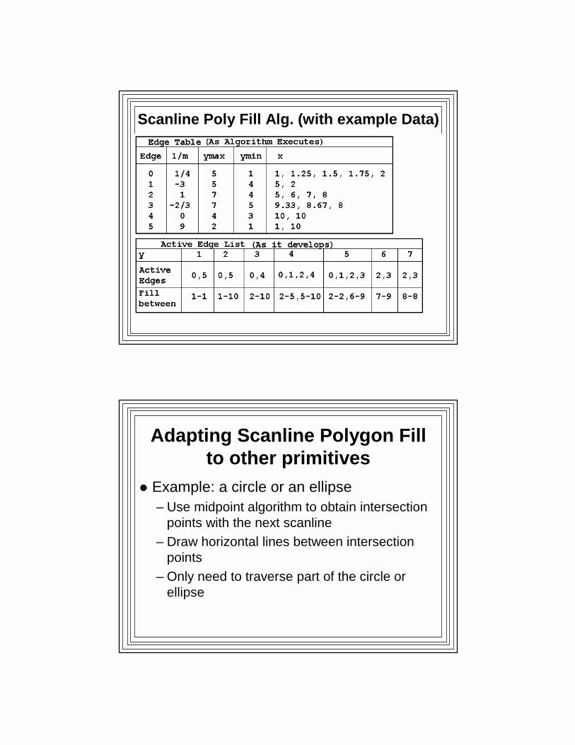
Scanline Poly Fill Alg. (with example Data)

Adapting Scanline Polygon Fill to other primitives

� Example: a circle or an ellipse– Use midpoint algorithm to obtain intersection

points with the next scanline– Draw horizontal lines between intersection

points– Only need to traverse part of the circle or

ellipse

Scanline Circle Fill Algorithm

The Scanline Boundary Fill Algorithm for Convex Polygons

Select a Seed Point (x,y)Push (x,y) onto StackWhile Stack is not empty:

Pop Stack (retrieve x,y)Fill current run y (iterate on x until borders are hit)Push left-most unfilled, nonborder pixel above

-->new "above" seedPush left-most unfilled, nonborder pixel below

-->new "below" seed

Demo of Scanline Polygon Fill Algorithm vs. Boundary Fill

Algorithm

� Polyfill Program– Does:

• Boundary Fill• Scanline Polygon Fill• Scanline Circle with a Pattern• Scanline Boundary Fill (Dino Demo)

Dino Demo of Scanline Boundary Fill Algorithm

Pattern Filling

� Represent fill pattern with a Pattern Matrix

� Replicate it across the area until covered by non-overlapping copies of the matrix– Called Tiling

Pattern Filling--Pattern Matrix

Using the Pattern Matrix

� Modify fill algorithm� As (x,y) pixel in area is examined:

if(pat_mat[x%W][y%H] == 1)SetPixel(x,y);

A More Efficient WayStore pat_matrix as a 1-D array of bytes or words, e.g., WxH

y%H --> byte or word in pat_matrixShift a mask by x%W

e.g. 10000000 for 8x8 pat_matrix--> position of bit in byte/word of pat_matrix

“AND” byte/word with shifted maskif result != 0, Set the pixel

Color Patterns

� Pattern Matrix contains color values� So read color value of pixel directly

from the Pattern Matrix:

SetPixel(x, y, pat_mat[x%W][y%H])

Moving the Filled Polygon� As done above, pattern doesn’t move

with polygon� Need to “anchor” pattern to polygon� Fix a polygon vertex as “pattern

reference point”, e.g., (x0,y0)If (pat_matrix[(x-x0)%W][(y-y0)%H]==1)

SetPixel(x,y)

� Now pattern moves with polygon

Pattern Filling--Pattern Matrix

OpenGL Line/Polygon Attributes� Line Width

– glLineWidth(width);• width: floating pt value rounded to nearest integer

� Line Style– glLineStipple(repeat factor, pattern);

• pattern: 16-bit integer describes style (1 on, 0 off)• repeat factor: integer expressing how many times

each bit in pattern repeats before next bit is applied – default 1

– Must activate Line Style feature• glEnable(GL_LINE_STIPPLE)

Other OpenGL Line Effects� Color Gradations

– Vary color smoothly between line endpoints– Assign different color to each endpoint

• System interpolates between colorsglShadeModel(GL_SMOOTH);glBegin(GL_LINES);

glColor3f(0.0, 0.0, 1.0); // one end blueglVertex2i(50, 50);glColor3f(1.0, 0.0, 0.0); // other end redglVertex2i(100, 100);

glEnd();

Area Fill in OpenGL

� Only available for convex polygons� Steps:

– Define fill pattern– Invoke polygon-fill routine– Activate polygon-fill feature in OpenGL– Describe the polygon(s) to be filled

OpenGL Pattern Fill� Default: convex polygon displayed in

solid color using current color setting� Pattern fill:

– Use a 32 X 32 bit mask• 1: pixel set to current color• 0: background color• Glubyte fp[ ] = {0xff,0xff,0xff,0xff,0,0,0,0…}

– Bottom row first

– glPolygonStipple(fp);– glEnable(GL_POLYGON_STIPPLE);

OpenGL Interpolation Patterns� Can assign different colors to vertices� OpenGL will interpolate interior colors

glShadeModel(GL_SMOOTH);glBegin(GL_POLYGON)

glColor3f(0.0, 0.0, 1.0); // one vertex blueglVertex2i(25, 25);glColor3f(1.0, 0.0, 0.0); // another redglVertex2i(75, 75);glColor3f(0.0,1.0, 0.0); // last one greenglVertex2i(75, 25);

glEnd();

Geometric Transformations� Moving objects relative to a stationary

coordinate system� Common transformations:

– Translation– Rotation– Scaling

� Implemented using vectors and matrices

Quick Review of Matrix Algebra

� Matrix--a rectangular array of numbers� aij: element at row i and column j� Dimension: m x n

m = number of rowsn = number of columns

A Matrix

Vectors and Scalars

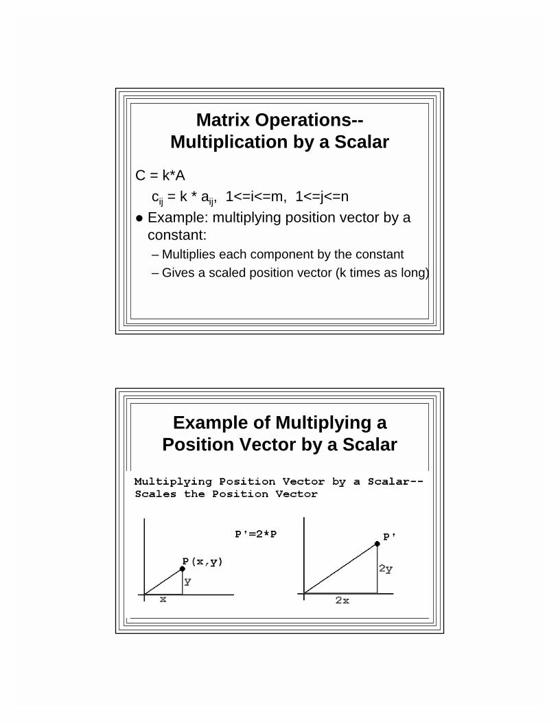
Matrix Operations--Multiplication by a Scalar

C = k*Acij = k * aij, 1<=i<=m, 1<=j<=n

� Example: multiplying position vector by a constant:– Multiplies each component by the constant– Gives a scaled position vector (k times as long)

Example of Multiplying a Position Vector by a Scalar

Adding two Matrices

� Must have the same dimension� C = A + B

cij = aij + bij, 1<=i<=m, 1<=j<=n� Example: adding two position vectors

– Add the components– Gives a vector equal to the net

displacement

Adding two Position Vectors: Result is the Net Displacement

Multiplying Two Matrices� m x n = (m x p) * (p x n)� C = A * B

� cij = Σ aik*bkj , 1<=k<=p� In other words:

– To get element in row i, column j• Multiply each element in row i by each

corresponding element in column j• Add the partial products

Matrix Multiplication An Example

Multipy a Vector by a Matrix� V’ = A*V� If V is a m-dimensional column vector,

A must be an m x m matrix

� V’i = Σ aik * vk, 1<=k<=m– So to get element i of product vector:

• Multiply each row i matrix element by each corresponding element of the vector

• Add the partial products

An Example

Geometrical Transformations

� Alter or move objects on screen� Affine Transformations:

– Each transformed coordinate is a linear combination of the original coordinates

– Preserve straight lines� Transform points in the object

– Translation:• A Vector Sum

– Rotation and Scaling:• Matrix Multiplies

Translation: Moving Objects

Scaling: Sizing Objects

Scaling, continuedP’ = S*PP, P’ are 2D vectors, so S must be 2x2 matrixComponent equations:

x’ = sx*x, y’ = sy*y

Rotation about Origin

� Rotate point P by θ about origin� Rotated point is P’� Want to get P’ from P and θ� P’ = R*P� R is the rotation matrix� Look at components:

Rotation: X Component

Rotation: Y Component

Rotation: ResultP’ = R*PR must be a 2x2 matrixComponent equations:

x’ = x cos(θ) - y sin(θ)y’ = x sin(θ) + y cos(θ)

Transforming Objects

� For example, lines1. Transform every point & plot (too

slow)2. Transform endpoints, draw the line

• Since these transformations are affine, result is the transformed line

Composite Transformations� Successive transformations� e.g., scale then rotate an n-point object:

1. Scale points: P’ = S*P (n matrix multiplies)2. Rotate pts: P’’ = R*P’ (n matrix multiplies)But:

P’’ = R*(SP), & matrix multiplication is associativeP’’ = (R*S)*P = Mcomp*P

So Compute Mcomp = R*S (1 matrix mult.)P’’ = Mcomp*P (n matrix multiplies)n+1 multiplies vs. 2*n multiplies

Composite TransformationsAnother example: Rotate in place

center at (a,b)1. Translate to origin: T(-a.-b)2. Rotate: R(θ)3. Translate back: T(a,b)

Rotation in place:1. P’ = P + T12. P’’ = R*P’ = R*(P+T1)3. P’’’ = P’’+T3 = R*(P+T1) + T3Can’t be put into single matrix mult. form:

i.e., P’’’ != Tcomp * PBut we want to be able to do that!!

Problem is: translation--vector addrotation/scaling--matrix multiply

Homogeneous Coordinates� Redefine transformations so each is a

matrix multiply� Express each 2-D Cartesian point as a

triple:– A 3-D vector in a “homogeneous”

coordinate systemx xh where we define:

y yh xh = w*x,

w yh = w*y

� Each (x,y) maps to an infinite number of homogeneous 3-D points, depending on w

� Take w=1� Look at our affine geometric

transformations

Homogeneous Translations

Homogeneous Scaling (wrt origin)

Homogeneous Rotation (about origin)

Composite Transformations with Homogeneous Coordinates

� All transformations implemented as homogeneous matrix multiplies

� Assume transformations T1, then T2, then T3:Homogeneous matrices are T1, T2, T3P’ = T1*PP’’ = T2*P’ = T2*(T1*P) = (T2*T1)*PP’’=T3*P’’=T3*((T2*T1)*P)=(T3*T2*T1)*PComposite transformation: T = T3*T2*T1Compute T just once!

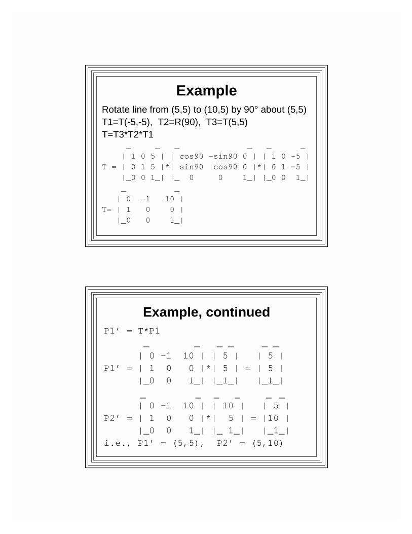
ExampleRotate line from (5,5) to (10,5) by 90° about (5,5)T1=T(-5,-5), T2=R(90), T3=T(5,5)T=T3*T2*T1

_ _ _ _ _ _

| 1 0 5 | | cos90 -sin90 0 | | 1 0 –5 |T = | 0 1 5 |*| sin90 cos90 0 |*| 0 1 –5 |

|_0 0 1_| |_ 0 0 1_| |_0 0 1_|

_ _

| 0 -1 10 |T= | 1 0 0 |

|_0 0 1_|

Example, continuedP1’ = T*P1

_ _ _ _ _ _| 0 -1 10 | | 5 | | 5 |

P1’ = | 1 0 0 |*| 5 | = | 5 ||_0 0 1_| |_1_| |_1_|

_ _ _ _ _ _| 0 -1 10 | | 10 | | 5 |

P2’ = | 1 0 0 |*| 5 | = |10 ||_0 0 1_| |_ 1_| |_1_|

i.e., P1’ = (5,5), P2’ = (5,10)

Setting Up a General 2D Geometric Transformation

Package

Multiplying a matrix & a vector: General 3D Formulation

_ _ _ _ _ _

| x’ | | a0 a1 a2 | | x |

| y’ | = | a3 a4 a5 | * | y |

|_z’_| |_a6 a7 a8_| |_z_|

So: x’ = a0*x + a1*y + a2*z

y’ = a3*x + a4*y + a5*z

z’ = a6*x + a7*y + a8*z

(9 multiplies and 6 adds)

Multiplying a matrix & a vector: Homogeneous Form

_ _ _ _ _ _

| x’ | | a0 a1 a2 | | x |

| y’ | = | a3 a4 a5 | * | y |

|_1 _| |_0 0 1 _| |_1_|

So: x’ = a0*x + a1*y + a2

y’ = a3*x + a4*y + a5

(4 multiplies and 4 adds)

MUCH MORE EFFICIENT!

Multiplying 2 3D Matrices: General 3D Formulation

_ _ _ _ _ _

| c0 c1 c2 | | a0 a1 a2 | | b0 b1 b2 |

| c3 c4 c5 |=| a3 a4 a5 |*| b3 b4 b5 |

|_c6 c7 c8_| |_a6 a7 a8_| |_b6 b7 b8_|

So: c0 = a0*b0 + a1*b3 + a2*b6

Eight more similar equations

(27 multiplies and 18 adds)

Multiplying 2 3D Matrices: Homogeneous Form

_ _ _ _ _ _| c0 c1 c2 | | a0 a1 a2 | | b0 b1 b2 || c3 c4 c5 |=| a3 a4 a5 |*| b3 b4 b5 ||_0 0 1 _| |_0 0 1 _| |_0 0 1 _|So: c0 = a0*b0 + a1*b3 + 0

(Similar equations for c1, c3, c4)

And: c2 = a0*b2 + a1*b5 +a2(Similar equation for c5)

(12 multiplies and 8 adds)MUCH MORE EFFICIENT!

Much Better to Implement our Own Transformation Package� In general, obtain transformed point P'

from original point P:� P' = M * P� Set up a a set of functions that will

transform points� Then devise other functions to do

transformations on polygons– since a polygon is an array of points

� Store the 6 nontrivial homogeneous transformation elements in a 1-D array A– The elements are a[i]

• a[0], a[1], a[2], a[3], a[4], a[5]

� Then represent any geometric transformation with the following matrix:

_ _| a[0] a[1] a[2] |

M = | a[3] a[4] a[5] ||_ 0 0 1 _|

� Define the following functions:– Enables us to set up and transform

points and polygons:settranslate(double a[6], double dx, double dy); // set xlate matrixsetscale(double a[6], double sx, double sy); // set scaling matrixsetrotate(double a[6], double theta); // set rotation matrixcombine(double c[6], double a[6], double b[6]); // C = A * Bxformcoord(double c[6], DPOINT vi, DPOINT* vo); // Vo=C*Vixformpoly(int n, DPOINT inpts[], DPOINT outpts[], double t[6]);

� The “set” functions take parameters that define the translation, scaling, rotation and compute the transformation matrix elements a[i]

� The combine() function computes the composite transformation matrix elements of the matrix C which is equivalent to the multiplication of transformation matrices A and B (C = A * B)

� The xformcoord(c[ ],Vi,Vo) function – Takes an input DPOINT (Vi, with x,y

coordinates)– Generates an output DPOINT (Vo, with x',y'

coordinates)– Result of the transformation represented by

matrix C whose elements are c[i]

� The xformpoly(n,ipts[ ],opts[ ],t[ ]) function– takes an array of input DPOINTs (an input

polygon)– and a transformation represented by matrix

elements t[i]– generates an array of ouput DPOINTs (an

output polygon)• result of applying the transformation t[ ] to the

points ipts[ ]– will make n calls to xformcoord()

• n = number of points in input polygon

An Example--Rotating a Polygon about one of its

Vertices by Angle θθθθ� Rotation about (dx,dy) can be achieved by

the composite transformation:1. Translate so vertex is at origin (-dx,-dy);

Matrix T12. Rotate about origin by θ; Matrix R3. Translate back (+dx,+dy); Matrix T2

� The composite transformation matrix would be: T = T2*R*T1

Some Sample Code: Rotating a Polygon about a

Vertex

Example Code: rotating a polygon about a vertex

DPOINT p[4]; // input polygon DPOINT px[4]; // transformed polygonint n=4; // number of verticesint pts[ ]={0,0,50,0,50,70,0,70}; // poly vertex coordinatesfloat theta=30; // the angle of rotationdouble dx=50,dy=70; // rotate about this vertexdouble xlate[6]; // the transformation 'matrices'double rotate[6];double temp[6];double final[6];

for (int i=0; i<n; i++) // set up the input polygon{ p[i].x=pts[2*i];

p[i].y=pts[2*i+1]; }Polygon(p,n); // draw original polygonsettranslate(xlate,-dx,-dy); // set up T1 trans matrixsetrotate(rotate,theta); // set up R rotaton matrixcombine (temp,rotate,xlate); // compute R*T1 &...

// save in tempsettranslate(xlate,dx,dy); // set up T2 trans matrixcombine(final,xlate,temp); // compute T2*(R*T1) &...

// save in finalxformpoly(n,p,px,final); // get transformed polygon pxPolygon(px,n); // draw transformed polygon

Setting Up More General Polygon Transformation Routines

� trans_poly() could translate a polygon by tx,ty

� rotate_poly() could rotate a polygon by θabout point (tx,ty)

� scale_poly() could scale a polygon by sx, sy wrt (tx,ty)

� These would make calls to previously defined functions

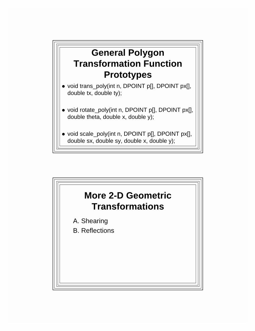
General Polygon Transformation Function

Prototypes� void trans_poly(int n, DPOINT p[], DPOINT px[],

double tx, double ty);

� void rotate_poly(int n, DPOINT p[], DPOINT px[], double theta, double x, double y);

� void scale_poly(int n, DPOINT p[], DPOINT px[], double sx, double sy, double x, double y);

More 2-D Geometric Transformations

A. ShearingB. Reflections

Other 2D Affine Transformations� Shearing (in x direction)

– Move all points in object in x direction an amount proportional to y

– Proportionality factor: • shx (x shearing factor)

– Equations:y’ = y

x’ = x + shx*y |1 shx 0 |

P’ = SHX*P SHX = |0 1 0 |

|0 0 1 |

– Move all points in object in y direction an amount proportional to x

– Proportionality factor: • shy (y shearing factor)

– Equations:x’ = x

y’ = shy*x + y |1 0 0 |

P’ = SHX*P SHX = |shy 1 0 |

|0 0 1 |

Shearing in y Direction

Reflections

� Reflect through originx --> -xy--> -yEquations:

x’ = -xy’ = -y |-1 0 0 |P’ = Ro*P Ro = | 0 -1 0 |

| 0 0 1 |

Reflect Across y-axis

y --> yx --> -x

Equations:x’ = -x |-1 0 0 |

y’ = y Ry = | 0 1 0 |

P’ = Ry*P | 0 0 1 |

Reflect Across Arbitrary LineGiven line endpoints: (x1,y1), (x2,y2)1. Translate by (-x1,-y1) [endpoint at origin]2. Rotate by φ [line coincides with y-axis]3. Reflect across y-axis4. Rotate by -φ5. Translate by (x1,y1)6. Composite transformation:

T = T(x1,y1)*R(-φ)*Ry*R(φ)*T(-x1,-y1)

Reflect Across a LineEndpoints (x1,y1), (x2,y2)

Coordinate System Transformations� Geometric Transformations:

– Move object relative to stationary coordinate system (observer)

� Coordinate System Transformation:– Move coordinate system (observer) & hold

objects stationary– Two common types

• Coordinate System translation• Coordinate System rotation

– Related to Geometric Transformations

Coordinate System Translation

Coordinate System Rotation