MATLAB and Octave

An Introduction

INTRODUCTION

Octave and MATLAB are high-level languages, primarily intended for numerical computations.

They provide a convenient command line interface for solving linear and nonlinear problems numerically.

They can also be used for prototyping and performing other numerical experiments.

Octave

MATLAB is a proprietary product that requires a license.

Octave is freely redistributable software. You may redistribute it and/or modify it under the terms of the GNU General Public License as published by the Free Software Foundation.

This document corresponds to Octave version 2.0.13.

Starting Octave

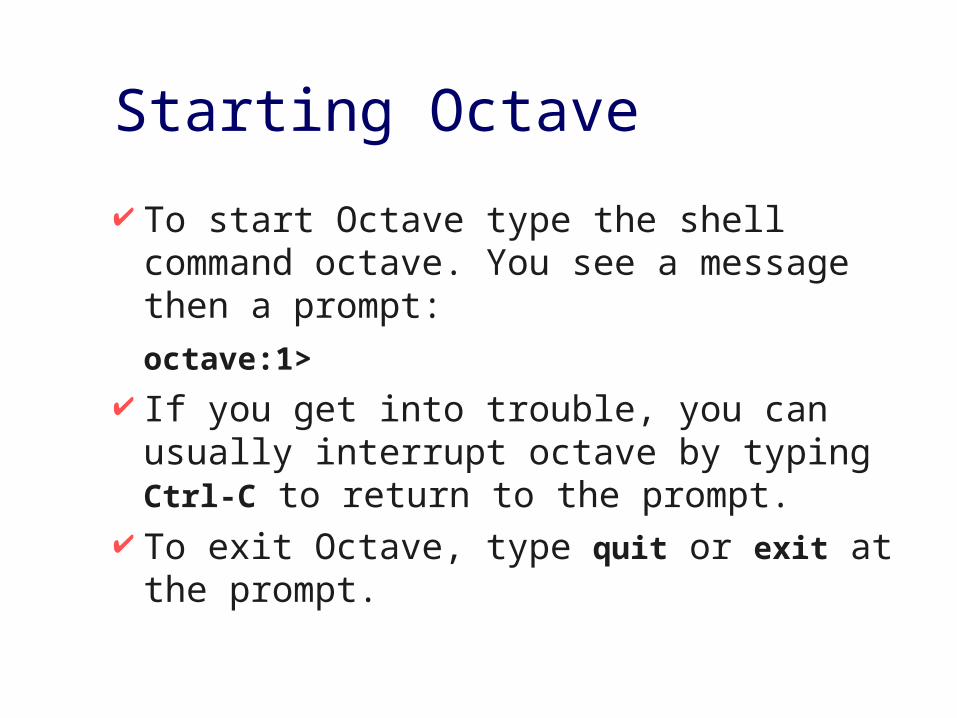
To start Octave type the shell command octave. You see a message then a prompt:

octave:1> If you get into trouble, you can usually

interrupt octave by typing Ctrl-C to return to the prompt.

To exit Octave, type quit or exit at the prompt.

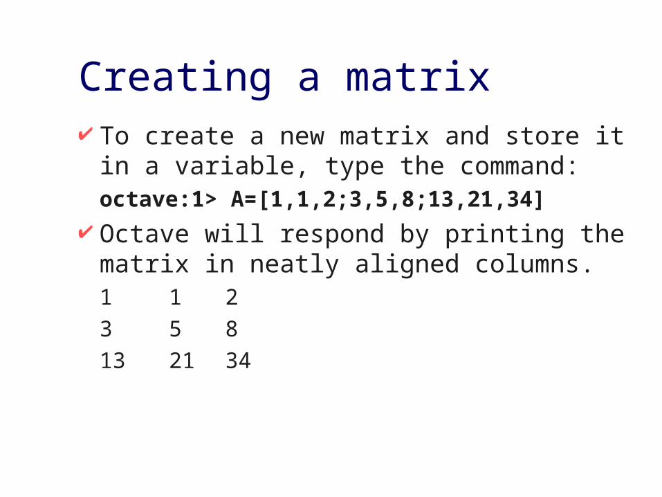
Creating a matrix To create a new matrix and store it in a

variable, type the command:octave:1> A=[1,1,2;3,5,8;13,21,34]

Octave will respond by printing the matrix in neatly aligned columns.

1 1 2

3 5 8

13 21 34

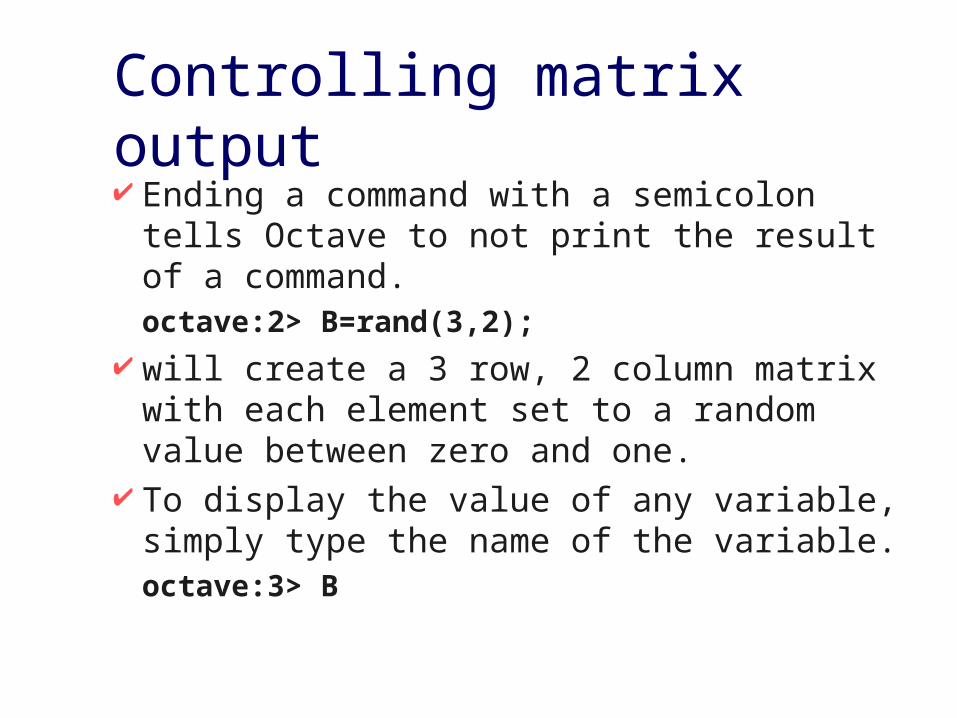
Controlling matrix output Ending a command with a semicolon tells

Octave to not print the result of a command. octave:2> B=rand(3,2);

will create a 3 row, 2 column matrix with each element set to a random value between zero and one.

To display the value of any variable, simply type the name of the variable. octave:3> B

Matrix arithmetic

Octave has a convenient operator notation for performing matrix arithmetic. To multiply the matrix a by a scalar, type: octave:4> 2*A

To multiply the two matrices A and B, type: octave:5> A*B

To form the matrix product type:octave:6> A’*A

Solving linear equations

To solve the set of linear equations Ax=b, use the left division operator \ :octave:7> A\b

This is conceptually equivalent to inverting the A matrix but avoids computing the inverse of a matrix directly.

If the coefficient matrix is singular, Octave will print a warning message.

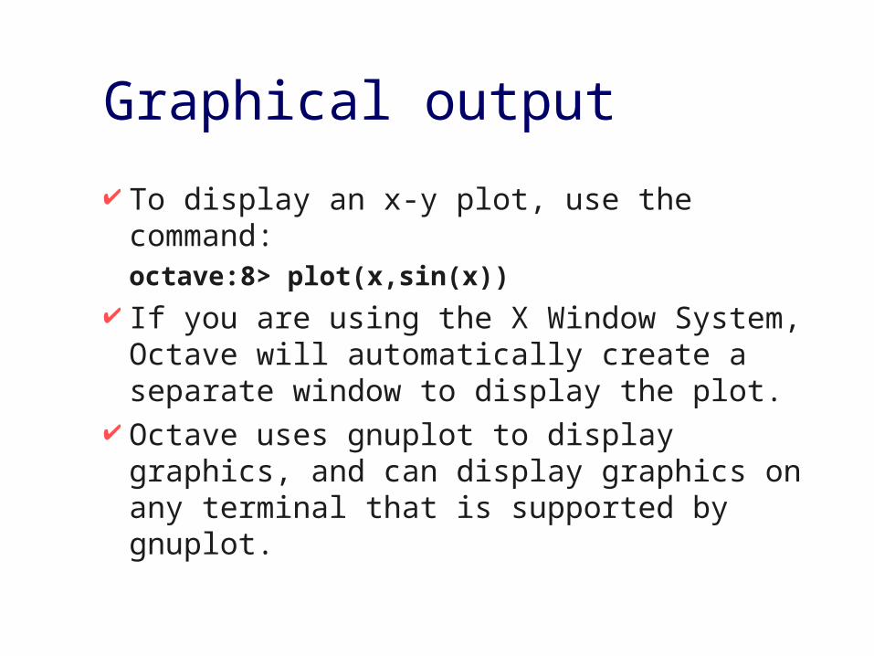
Graphical output

To display an x-y plot, use the command: octave:8> plot(x,sin(x))

If you are using the X Window System, Octave will automatically create a separate window to display the plot.

Octave uses gnuplot to display graphics, and can display graphics on any terminal that is supported by gnuplot.

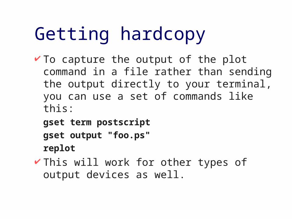
Getting hardcopy To capture the output of the plot command in a

file rather than sending the output directly to your terminal, you can use a set of commands like this: gset term postscript

gset output "foo.ps"

replot

This will work for other types of output devices as well.

DATA TYPES

The standard built-in data types are – real and complex scalars, – real and complex matrices, – ranges, – character strings, – a data structure type.

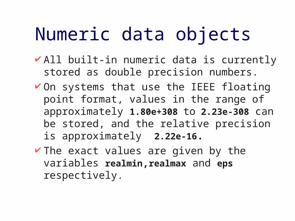
Numeric data objects All built-in numeric data is currently stored as

double precision numbers. On systems that use the IEEE floating point

format, values in the range of approximately 1.80e+308 to 2.23e-308 can be stored, and the relative precision is approximately 2.22e-16.

The exact values are given by the variables realmin,realmax and eps respectively.

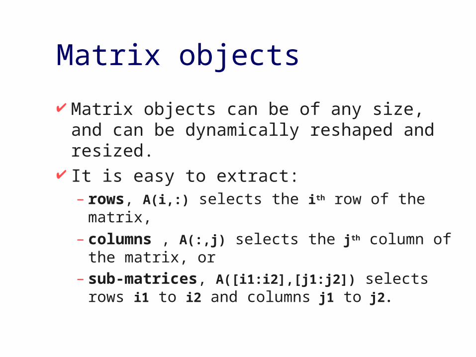
Matrix objects

Matrix objects can be of any size, and can be dynamically reshaped and resized.

It is easy to extract:– rows, A(i,:) selects the ith row of the matrix, – columns , A(:,j) selects the jth column of the

matrix, or – sub-matrices, A([i1:i2],[j1:j2]) selects

rows i1 to i2 and columns j1 to j2.

Range objects

A range expression is defined by the value of the first element in the range, an optional value for the increment between elements, and a maximum value which the elements of the range will not exceed.

The base, increment, and limit are separated by colons and may contain any arithmetic expressions and function calls.

String objects

A character string in Octave consists of a sequence of characters enclosed in either double-quote or single-quote marks.

Internally, Octave currently stores strings as matrices of characters.

All the indexing operations that work for matrix objects also work for strings.

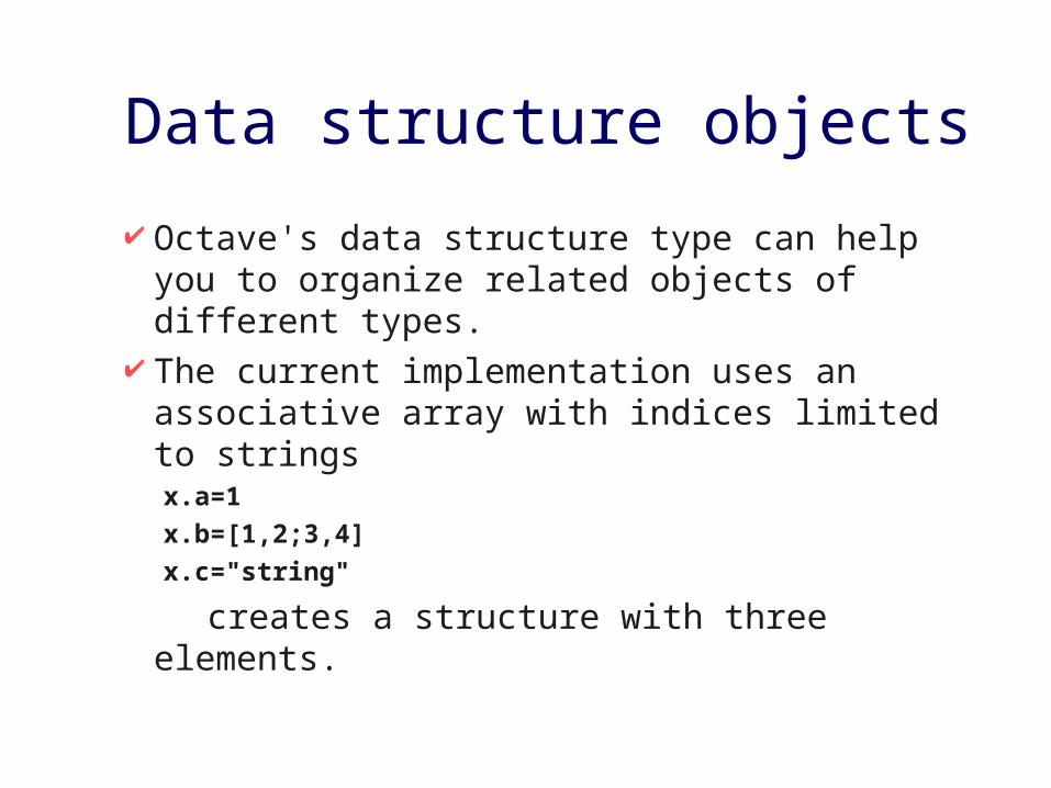
Data structure objects

Octave's data structure type can help you to organize related objects of different types.

The current implementation uses an associative array with indices limited to stringsx.a=1

x.b=[1,2;3,4]

x.c="string"

creates a structure with three elements.

Object sizes

A group of functions allow you to display the size of a variable or expression.

These functions are defined for all objects. They return -1 when the operation doesn't make sense.

For example, the data structure type doesn't have rows or columns, so the rows and columns functions return -1 for structure arguments.

Object size functions

columns(A) – Return the number of columns of A.

rows(A) – Return the number of rows of A.

length(A) – Return the number of rows of A or the number

of columns of A, whichever is larger.

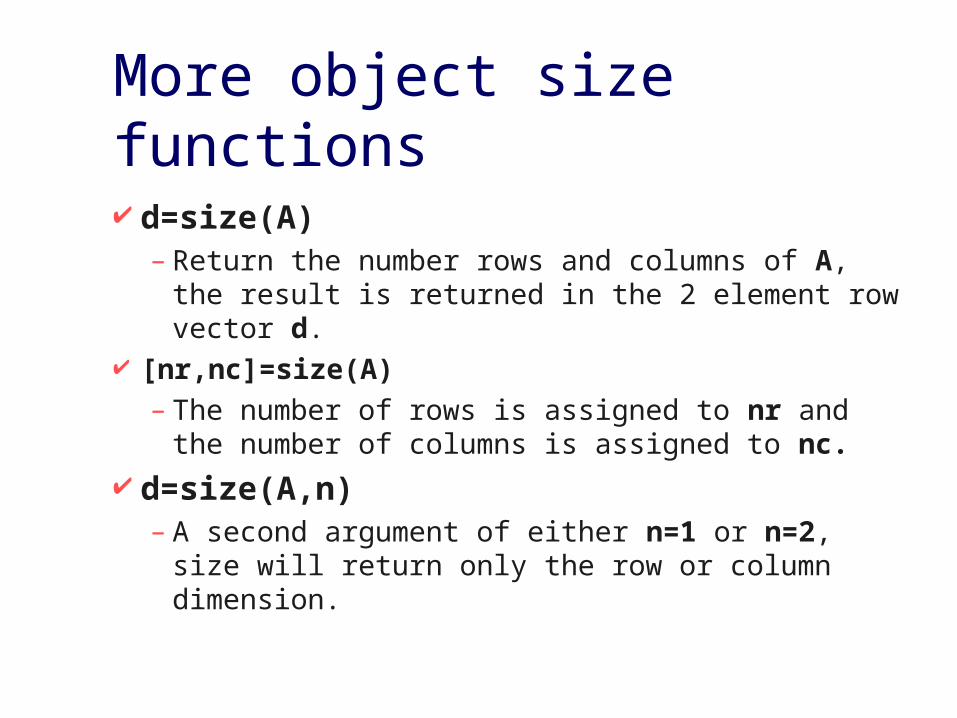
More object size functions

d=size(A) – Return the number rows and columns of A, the

result is returned in the 2 element row vector d. [nr,nc]=size(A)

– The number of rows is assigned to nr and the number of columns is assigned to nc.

d=size(A,n)– A second argument of either n=1 or n=2, size will

return only the row or column dimension.

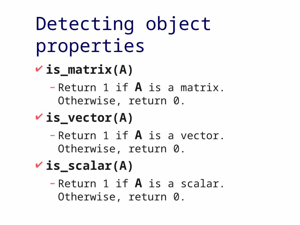
Detecting object properties

is_matrix(A) – Return 1 if A is a matrix. Otherwise, return 0.

is_vector(A) – Return 1 if A is a vector. Otherwise, return 0.

is_scalar(A) – Return 1 if A is a scalar. Otherwise, return 0.

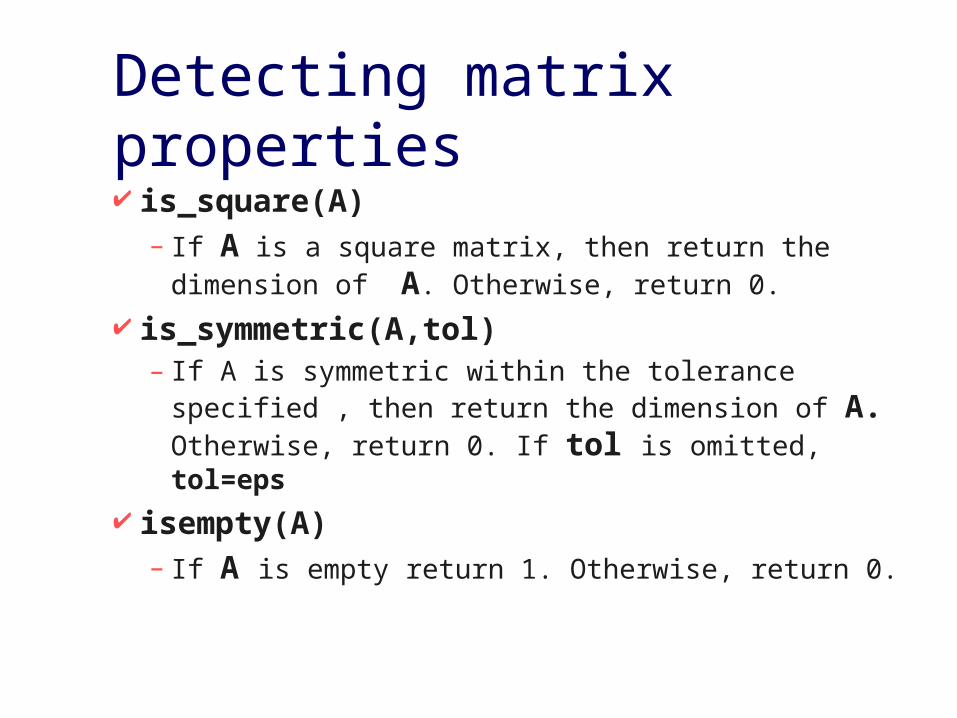
Detecting matrix properties is_square(A)

– If A is a square matrix, then return the dimension of A. Otherwise, return 0.

is_symmetric(A,tol) – If A is symmetric within the tolerance specified , then

return the dimension of A. Otherwise, return 0. If tol is omitted, tol=eps

isempty(A) – If A is empty return 1. Otherwise, return 0.

Range definition

The range 1:5– defines the set of values [1,2,3,4,5].

The range 1:2:5– defines the set of values [1,3,5].

The range 1:3:5– defines the set of values [1,4].

The range 5:-3:1– defines the set of values [5,2].

More about ranges

Note that the upper (or lower, if the increment is negative) bound on the range is not always included in the set of values.

Ranges defined by floating point values can produce surprising results because floating point arithmetic is used.

If it is important to include the endpoints of a range and the number of elements is known, use the linspace() function.

Special matrix object eye() eye(x)

– If invoked with a single scalar argument, eye returns a square identity matrix with the dimension specified.

eye(n,m) or eye(size(A))– If you supply two scalar arguments, eye takes them

to be the number of rows and columns.

eye– Calling eye with no arguments is equivalent to calling

it with an argument of 1.

Special matrix object ones() ones(x)

– If invoked with a single scalar argument, ones returns a square matrix of 1’s with the dimension specified.

ones(n,m) or ones(size(A))– If you supply two scalar arguments, ones takes them

to be the number of rows and columns.

ones– Calling ones with no arguments is equivalent to

calling it with an argument of 1.

Special matrix object zeros() zeros(x)

– If invoked with a single scalar argument, zeros returns a square matrix of 0’s with the dimension specified.

zeros(n,m) or zeros(size(A))– If you supply two scalar arguments, zeros takes them

to be the number of rows and columns.

zeros– Calling zeros with no arguments is equivalent to

calling it with an argument of 1.

Special matrix object rand() rand(x)

– If invoked with a single scalar argument, rand returns a square matrix of random numbers between 0 and 1 with the dimension specified.

rand(n,m) or rand(size(A))– If you supply two scalar arguments, rand takes them to

be the number of rows and columns.

rand– Calling rand with no arguments is equivalent to calling it

with an argument of 1.

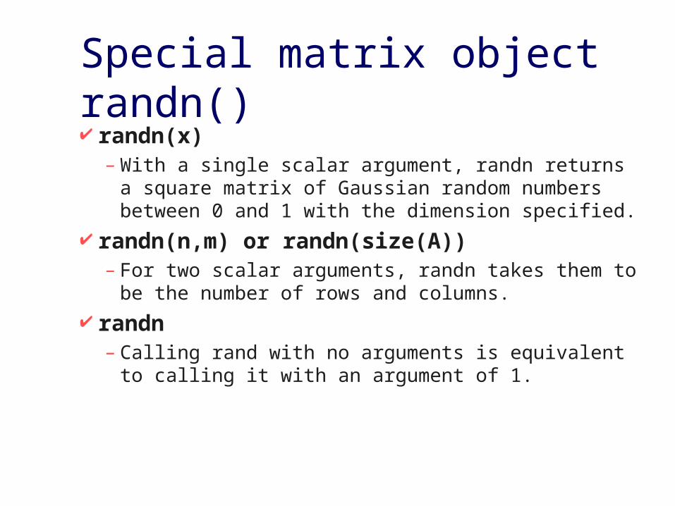
Special matrix object randn() randn(x)

– With a single scalar argument, randn returns a square matrix of Gaussian random numbers between 0 and 1 with the dimension specified.

randn(n,m) or randn(size(A))– For two scalar arguments, randn takes them to be the

number of rows and columns.

randn– Calling rand with no arguments is equivalent to calling it

with an argument of 1.

Random number seeds Normally, rand and randn obtain their initial

seeds from the system clock,so that the sequence of random numbers is not the same each time you run Octave.

To allow generation of identical sequences, rand and randn allow the random number seed to be specified.

rand(‘seed’,value) or

randn(‘seed’,value)

STRINGS

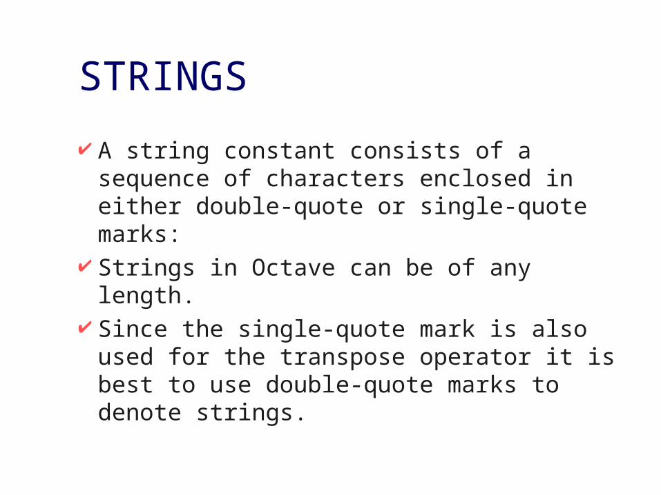
A string constant consists of a sequence of characters enclosed in either double-quote or single-quote marks:

Strings in Octave can be of any length. Since the single-quote mark is also used for

the transpose operator it is best to use double-quote marks to denote strings.

Literals

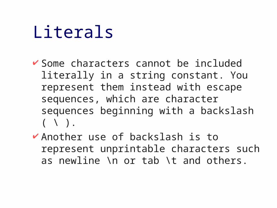
Some characters cannot be included literally in a string constant. You represent them instead with escape sequences, which are character sequences beginning with a backslash ( \ ).

Another use of backslash is to represent unprintable characters such as newline \n or tab \t and others.

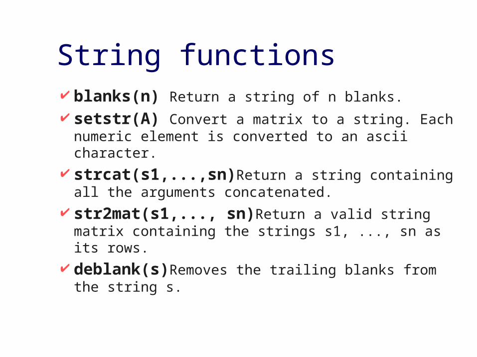
String functions blanks(n) Return a string of n blanks. setstr(A) Convert a matrix to a string. Each

numeric element is converted to an ascii character. strcat(s1,...,sn)Return a string containing

all the arguments concatenated. str2mat(s1,..., sn)Return a valid string

matrix containing the strings s1, ..., sn as its rows. deblank(s)Removes the trailing blanks from the

string s.

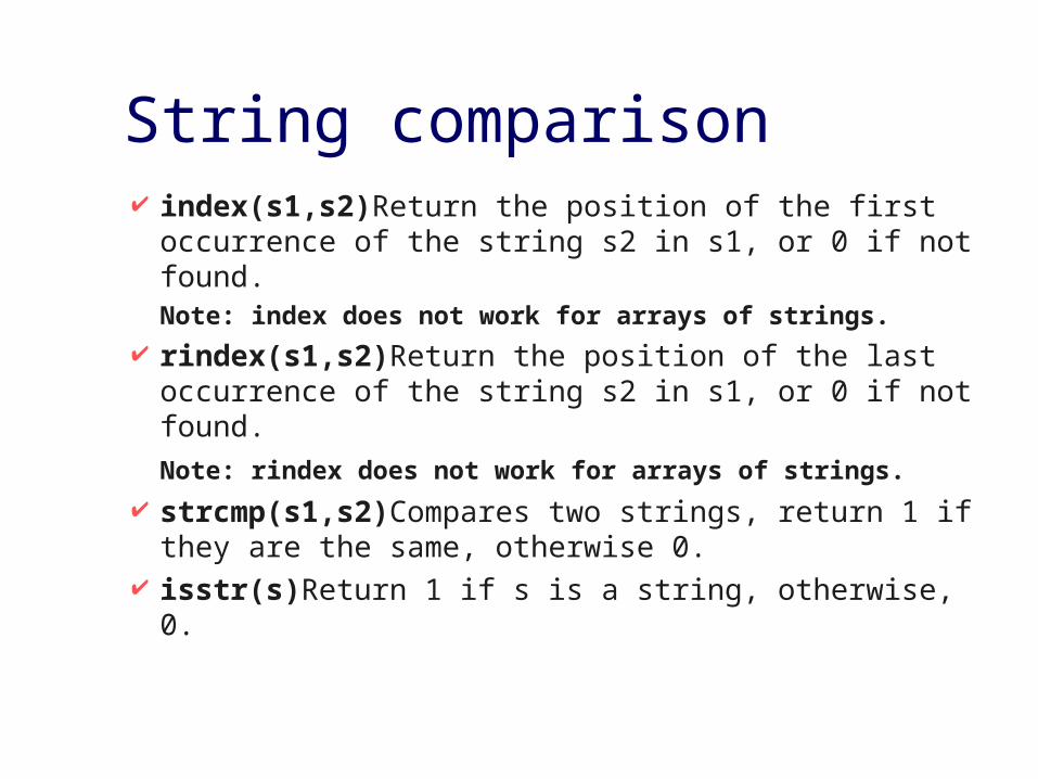
String comparison index(s1,s2)Return the position of the first

occurrence of the string s2 in s1, or 0 if not found. Note: index does not work for arrays of strings.

rindex(s1,s2)Return the position of the last occurrence of the string s2 in s1, or 0 if not found.

Note: rindex does not work for arrays of strings. strcmp(s1,s2)Compares two strings, return 1

if they are the same, otherwise 0. isstr(s)Return 1 if s is a string, otherwise, 0.

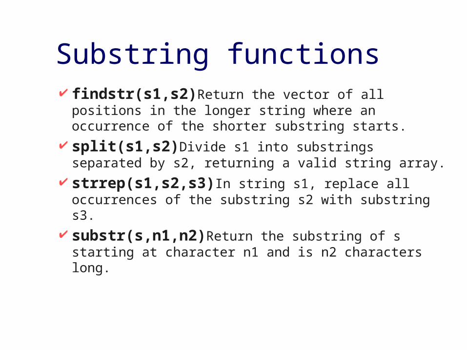
Substring functions findstr(s1,s2)Return the vector of all

positions in the longer string where an occurrence of the shorter substring starts.

split(s1,s2)Divide s1 into substrings separated by s2, returning a valid string array.

strrep(s1,s2,s3)In string s1, replace all occurrences of the substring s2 with substring s3.

substr(s,n1,n2)Return the substring of s starting at character n1 and is n2 characters long.

String conversions bin2dec(s)Return a decimal number corresponding to the

binary number represented as a string of 0s and 1s.

dec2bin(n)Return a binary number as a string of 0s and 1s corresponding the non-negative decimal number n.

hex2dec(s)Return a decimal number corresponding to the hexadecimal number stored in the string s.

dec2hex(n)Return the hex number corresponding to the non-negative decimal number n, as a string.

str2num(s)Convert the string s to a number. num2str(n)Convert the number n to a string.

More string conversions toascii(s)Return ascii representation of s in a

matrix. tolower(s)Return a copy of the string s, with each

upper-case character replaced by the corresponding lower-case one; non-alphabetic characters are left unchanged.

toupper(s)Return a copy of the string s, with each lower-case character replaced by the corresponding upper-case one; non-alphabetic characters are left unchanged.

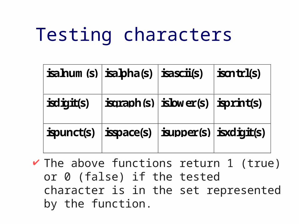
Testing characters

isalnum(s) isalpha(s) isascii(s) iscntrl(s)

isdigit(s) isgraph(s) islower(s) isprint(s)

ispunct(s) isspace(s) isupper(s) isxdigit(s)

The above functions return 1 (true) or 0 (false) if the tested character is in the set represented by the function.

VARIABLES Variables let you give names to values and refer

to them later. The name of an Octave variable must be a

sequence of letters, digits and underscores, but it may not begin with a digit.

There is no limit on the number of characters in a variable name.

Case is significant in variable names. The symbols a and A are distinct variables.

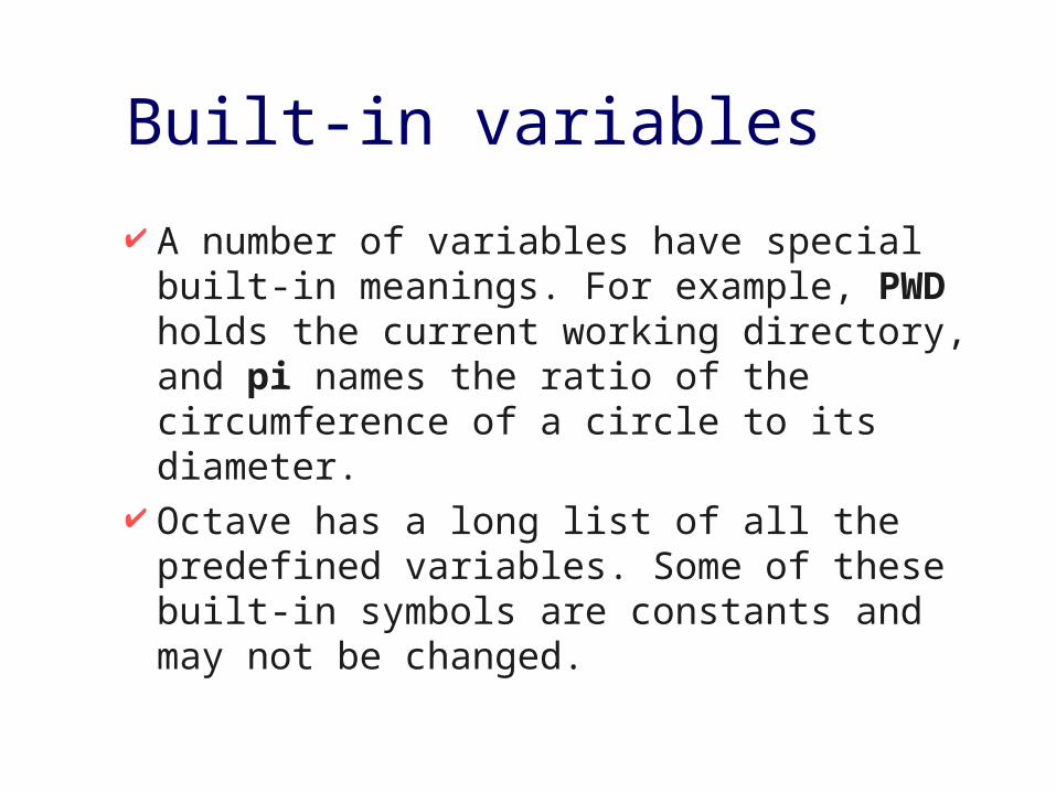
Built-in variables

A number of variables have special built-in meanings. For example, PWD holds the current working directory, and pi names the ratio of the circumference of a circle to its diameter.

Octave has a long list of all the predefined variables. Some of these built-in symbols are constants and may not be changed.

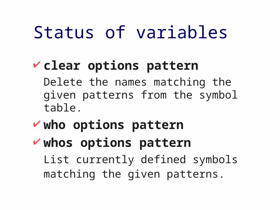
Status of variables

clear options pattern Delete the names matching the given patterns from the symbol table.

who options pattern whos options pattern

List currently defined symbols matching the given patterns.

Options

The following are valid options for the clear and who functions. They may be shortened to one character but may not be combined.

-a(ll) List all currently defined symbols. -b(uiltins) List built-in variables and functions. -f(unctions) List user-defined functions. -l(ong) Print a long listing of symbols -v(ariables) List user-defined variables.

EXPRESSIONS Expressions are the basic building block of statements

in Octave. – An expression evaluates to a value, which you can print, test,

store in a variable, pass to a function, or assign a new value to a variable with an assignment operator.

– An expression alone can serve as a statement. Most statements contain one or more expressions which specify data to be operated on.

– Expressions include variables, array references, constants, and function calls, as well as combinations of these with various operators.

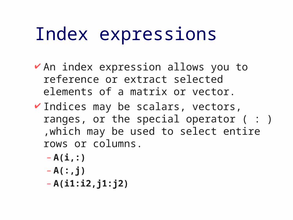
Index expressions

An index expression allows you to reference or extract selected elements of a matrix or vector.

Indices may be scalars, vectors, ranges, or the special operator ( : ) ,which may be used to select entire rows or columns. – A(i,:)– A(:,j)– A(i1:i2,j1:j2)

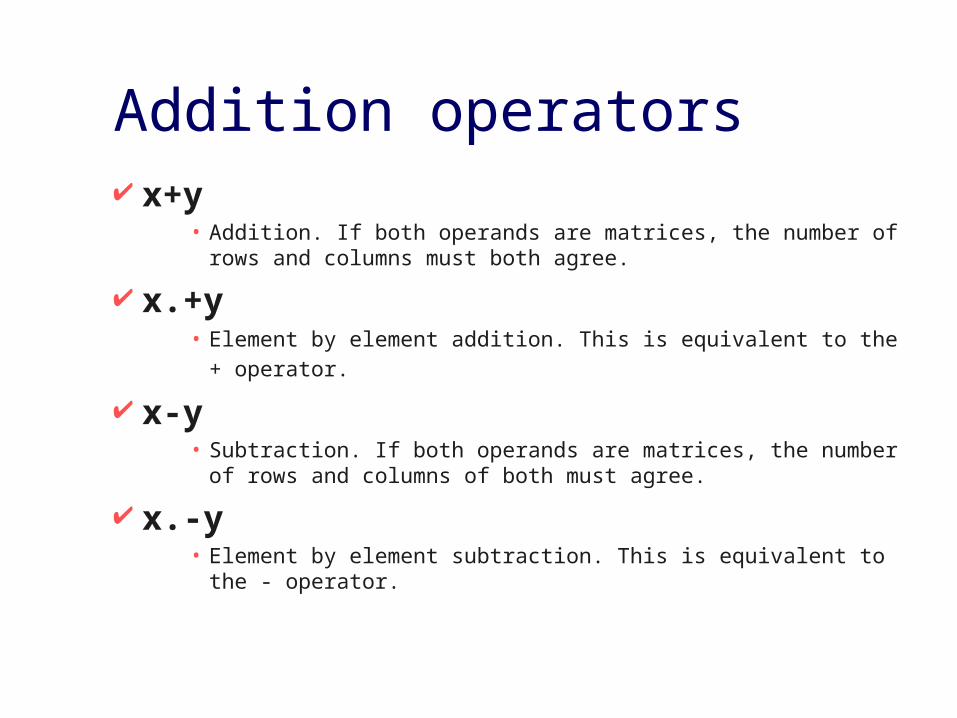
Addition operators x+y

• Addition. If both operands are matrices, the number of rows and columns must both agree.

x.+y • Element by element addition. This is equivalent to the + operator.

x-y • Subtraction. If both operands are matrices, the number of rows and

columns of both must agree.

x.-y • Element by element subtraction. This is equivalent to the - operator.

Multiplication operators

x*y • Matrix multiplication. The number of columns of x

must agree with the number of rows of y.

x.*y • Element by element multiplication. If both operands

are matrices, the number of rows and columns must both agree.

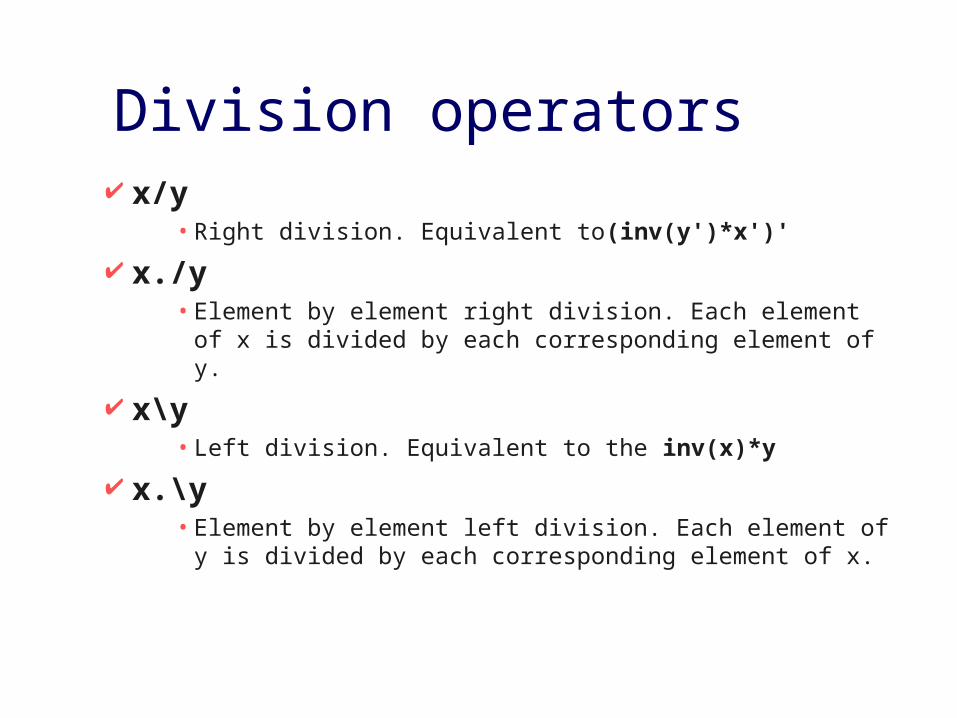
Division operators x/y

• Right division. Equivalent to(inv(y')*x')'

x./y • Element by element right division. Each element of x is

divided by each corresponding element of y.

x\y • Left division. Equivalent to the inv(x)*y

x.\y • Element by element left division. Each element of y is divided

by each corresponding element of x.

Power operators x^y or x**y

– Power operator. • x and y both scalar: returns x raised to the power y.

• x scalar, y is a square matrix : returns result using eigenvalue expansion.

• x is a square matrix and y scalar: returns result by repeated multiplication if y is an integer, else by eigenvalue expansion.

• x and y both matrices: returns an error.

x.^y or x.**y – Element by element power operator.

• If both operands are matrices, the number of rows and columns must both agree.

Unary operators +x or +x.

• A unary plus operator has no effect on the operand.

-x or -x.• Negation or element by element negation.

x' • Complex conjugate transpose. For real arguments, this is the

same as the transpose operator. For complex arguments, equivalent to conj(x.')

x.' • Element by element transpose.

Comparison operators Comparison operators compare numeric values

for relationships.– All of comparison operators return a value of 1 if the

comparison is true, or 0 if it is false. – For matrix values, the comparison is on an element-

by-element basis. •[1,2;3,4]==[1,3;2,4];ans=[1,0;0,1]

– For mixed scalar and matrix operands, the scalar is compared to each element in turn.•[1,2;3,4]==2;ans=[0,1;0,0]

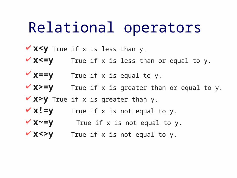
Relational operators x<y True if x is less than y. x<=y True if x is less than or equal to y.

x==y True if x is equal to y. x>=y True if x is greater than or equal to y.

x>y True if x is greater than y.

x!=y True if x is not equal to y.

x~=y True if x is not equal to y.

x<>y True if x is not equal to y.

Boolean expressions A boolean expression is a combination of

comparisons using the boolean operators "or" (|),"and" (&), and "not" (!).– Boolean expressions can be used wherever

comparison expressions can be used. – If a matrix value used as the condition it is only

true if all of its elements are nonzero. – Each element of an element-by-element boolean

expression has a numeric value (1 true, 0 false).

Boolean operators b1 & b2

• Elements of the result are true if both corresponding elements of b1 and b2 are true.

b1 | b2 • Elements of the result are true if either of the corresponding

elements of b1 or b2 is true.

!b ~b

• Each element of the result is true if the corresponding element of b is false.

Assignment expressions An assignment is an expression that stores a new

value into a variable. •z=1

Assignments can store string values also. •thing="food"•kind="good"•message=["this ",thing," is ",kind]

It is important to note that variables do not have permanent types. The type of a variable is whatever it happens to hold .

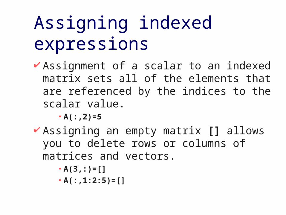
Assigning indexed expressions

Assignment of a scalar to an indexed matrix sets all of the elements that are referenced by the indices to the scalar value.

•A(:,2)=5

Assigning an empty matrix [] allows you to delete rows or columns of matrices and vectors.

•A(3,:)=[]•A(:,1:2:5)=[]

Assigning multiple variables An assignment is an expression, so it has a value.

Thus, z=1 as an expression has the value 1. One consequence of this is that you can write multiple assignments together:

•x=y=z=0

This is also true of assignments to lists, so the following are valid expressions

•[a,b,c]=[u,s,v]=svd(A)•[a,b,c,d]=[u,s,v]=svd(A)•[a,b]=[u,s,v]=svd(A)

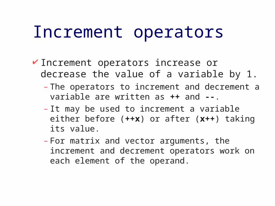
Increment operators

Increment operators increase or decrease the value of a variable by 1. – The operators to increment and decrement a

variable are written as ++ and --. – It may be used to increment a variable either

before (++x) or after (x++) taking its value. – For matrix and vector arguments, the increment

and decrement operators work on each element of the operand.

CONTROL STATEMENTS

Control statements control the flow of execution in programs. – All the control statements start with special

keywords – Each control statement has a corresponding end

keyword – The list of statements contained between the start

keyword the corresponding end keyword is called the body of a control statement.

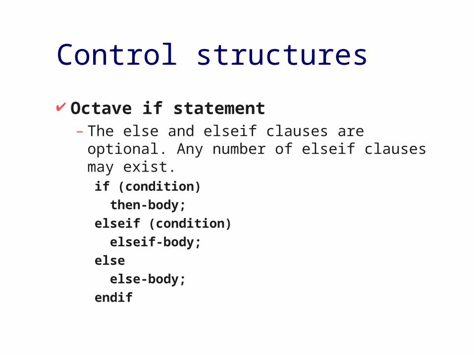
Control structures

Octave if statement– The else and elseif clauses are optional. Any number

of elseif clauses may exist.if (condition)

then-body;

elseif (condition)

elseif-body;

else

else-body;

endif

More control structures Octave switch statement

– Any number of case labels are possibleswitch expression

case label

command_list;

case label

command_list;

...

otherwise

command_list;

endswitch

More control structures Octave while statement

while (condition)

body;

endwhile

Octave for statementfor var = expression

body;

endfor

More control statements

The break statement – jumps out of the innermost for or while loop

that encloses it. The break statement may only be used within the body of a loop.

The continue statement – like break, is used only inside for or while

loops. It skips over the rest of the loop body, causing the next cycle around the loop to begin immediately.

FUNCTIONS A function is a name for a particular

calculation. For example, the function sqrt computes the square root of a number.

A fixed set of functions are built-in, which means they are available in every program. The sqrt function is a built-in function.

In addition, you can define your own functions.

Calling functions A function call expression is a function

name and list of arguments in parentheses. – The arguments are expressions which give the

data for function to operate on. – When there is more than one argument, they are

separated by commas. – If there are no arguments, you can omit the

parentheses.

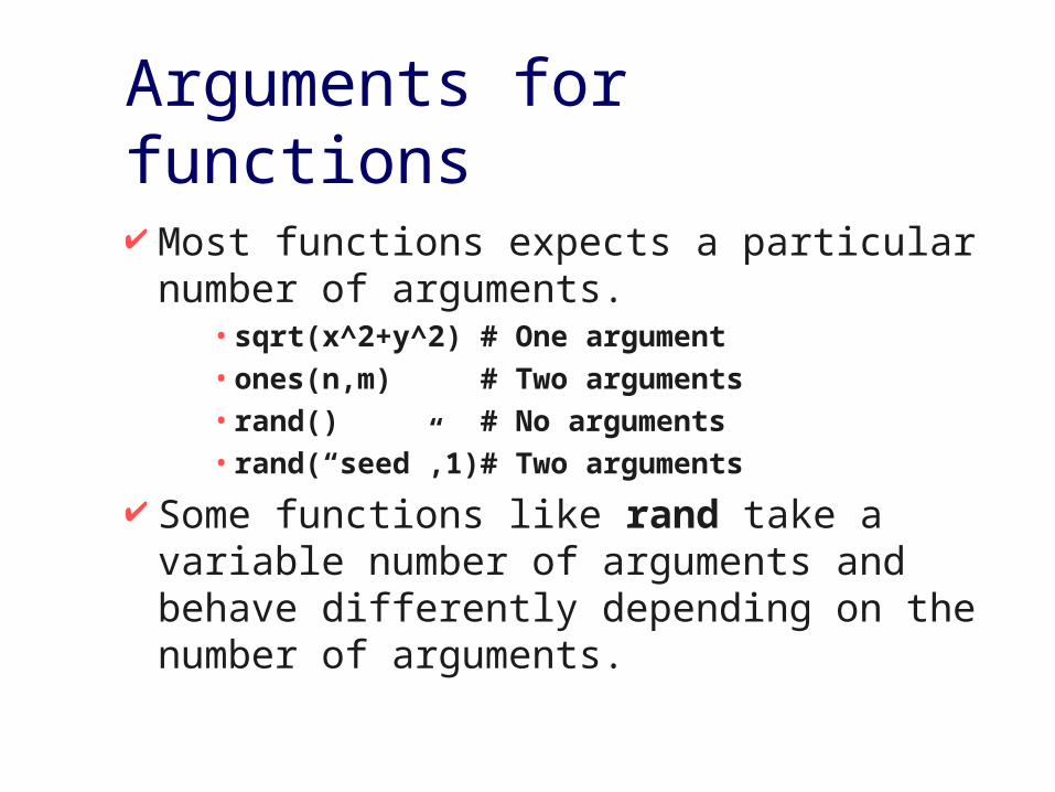
Arguments for functions

Most functions expects a particular number of arguments.

•sqrt(x^2+y^2) # One argument•ones(n,m) # Two arguments•rand() # No arguments•rand(“seed”,1)# Two arguments

Some functions like rand take a variable number of arguments and behave differently depending on the number of arguments.

Return values for functions

Most functions return one value

y=sqrt(x) Functions in Octave (in common with perl)

may return multiple values.

[u,s,v]=svd(A) computes the singular value decomposition of

the matrix A and assigns the three result matrices to u,s, and v.

Functions and script files

Complicated programs can often be simplified by defining functions.

Functions can be defined directly on the command line during interactive sessions.

Alternatively, functions can be created as external files, and can be called just like built-in functions.

Defining functions

In its simplest form, the definition of a function named name looks like this:

function name

body;

endfunction

A valid function name any valid variable name. The function body consists of expressions and

control statements.

Passing information to functions

Normally, you will want to pass some information to the functions you define.

function name(arg-list)

body;

endfunction

where arg-list is a comma-separated list of arguments. When the function is called, the argument names hold the values given in the call.

Returning information

In most cases, you will also want to get some information back from the functions you define.

function ret-var=name(arg-list)

body;

endfunction

The symbol ret-var is the name of the variable, defined within the function, that will hold the value to be returned.

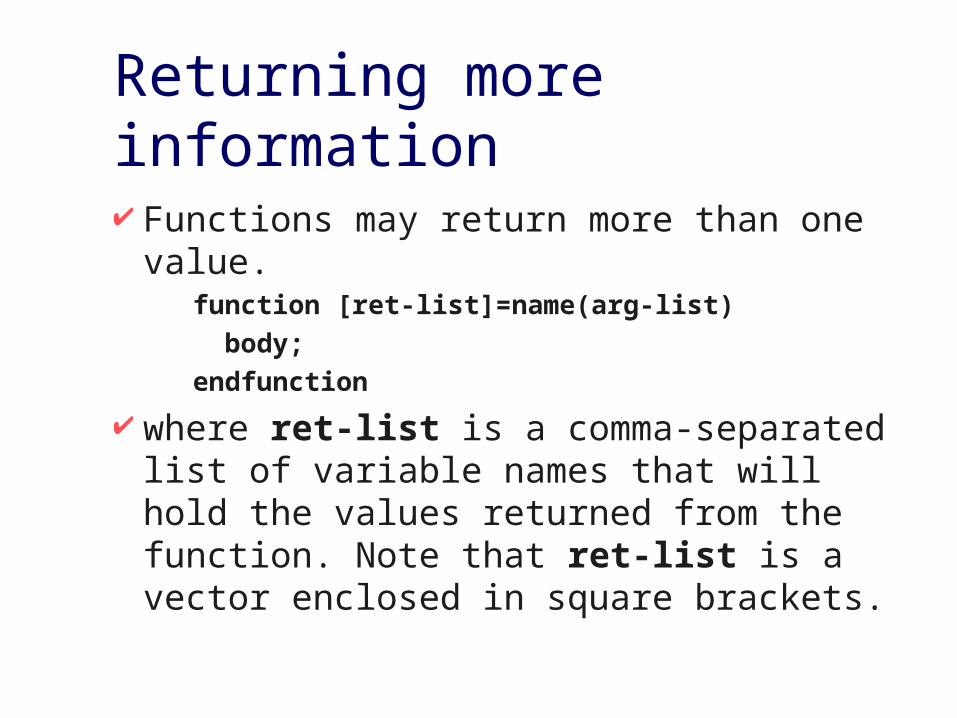
Returning more information

Functions may return more than one value. function [ret-list]=name(arg-list)

body;

endfunction

where ret-list is a comma-separated list of variable names that will hold the values returned from the function. Note that ret-list is a vector enclosed in square brackets.

Script files A script file is a file containing (almost) any

sequence of commands. • It is read and evaluated just as if you had typed each

command at the prompt. • It provides a way to store a sequence of commands that do

not logically belong inside a function. • Unlike a function file, a script file must not begin with the

keyword function.. • Variables named in a script file are not local variables, but

are in the same scope as the other variables entered at the prompt.

Function subdirectories (1)

audio for playing and recording sounds.

control for design and simulation ofautomatic control systems.

elfun elementary functions.

general miscellaneous matrixmanipulations.

image image processing tools.

io input-ouput functions.

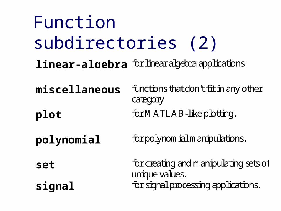
Function subdirectories (2)

linear-algebra for linear algebra applications

miscellaneous functions that don't fit in any othercategory

plot for MATLAB-like plotting.

polynomial for polynomial manipulations.

set for creating and manipulating sets ofunique values.

signal for signal processing applications.

Function subdirectories (3)

specfun special mainly inverse functions.

special-matrix to create special matrix forms.

statistics for statistical applications.

strings for string manipulations.

time for time keeping.

INPUT AND OUTPUT There are two distinct classes of input and output

functions. – The first set are modelled after the functions available in

MATLAB.– The second set are modelled after the standard I/O

library used by the C programming language and offer more flexibility and control.

When running interactively, Octave sends output that is more than one screen long to a paging program, such as less or more.

Terminal output

Since Octave normally prints the value of an expression as soon as it has been evaluated, the simplest of all I/O functions is a simple expression.

octave:1> pi

pi = 3.1416

This works well as long as it is acceptable to have the name of the variable (or the default ans) printed along with the value.

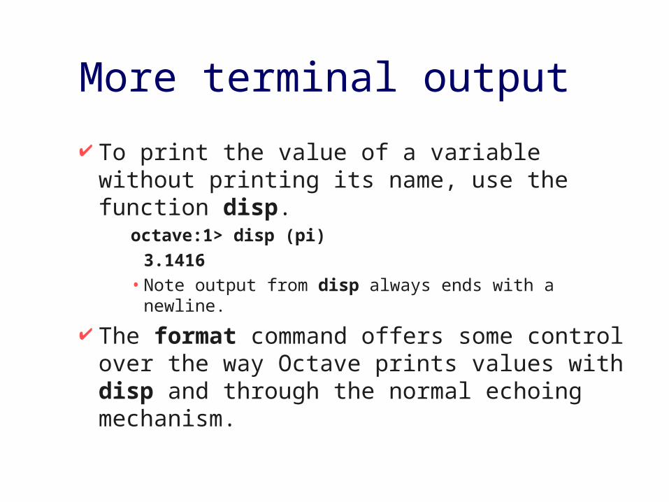
More terminal output

To print the value of a variable without printing its name, use the function disp.

octave:1> disp (pi)

3.1416• Note output from disp always ends with a newline.

The format command offers some control over the way Octave prints values with disp and through the normal echoing mechanism.

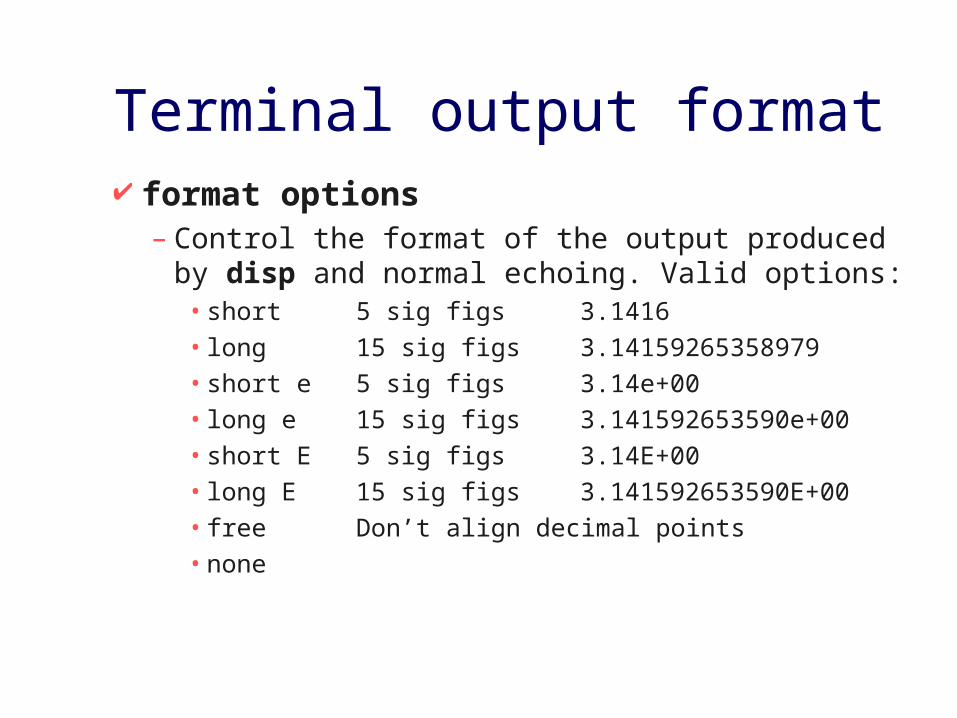
Terminal output format format options

– Control the format of the output produced by disp and normal echoing. Valid options:

• short 5 sig figs 3.1416

• long 15 sig figs 3.14159265358979

• short e 5 sig figs 3.14e+00

• long e 15 sig figs 3.141592653590e+00

• short E 5 sig figs 3.14E+00

• long E 15 sig figs 3.141592653590E+00

• free Don’t align decimal points

• none

More format options format options

• bank two decimal places

• + + for nonzero, space for zero elements

• hex 8 byte IEEE real

• bit 8 byte IEEE real

Terminal input Octave has three functions that make it easy to

prompt users for input. – input– menu– keyboard

The input and menu functions are used for managing an interactive dialog with a user.

The keyboard function is used for simple debugging.

Terminal input function input(prompt)

– Print a prompt and wait for user input. • The string entered by the user is evaluated as an

expression, so it may be a literal constant, a variable name, or any other valid expression.

input(prompt,"s") – Print a prompt and wait for user input.

• Return the string entered by the user directly, without evaluating it first.

Terminal menu function menu(title,opt1,...)

– Print a title string followed by a series of options. Each option will be printed along with a number. The return value is the number of the option selected by the user. Are you there

1. Yes

2. No

>

Terminal keyboard function keyboard(prompt)

– This function is used for simple debugging. When the keyboard function is executed, Octave prints a prompt and waits for user input. The default prompt is debug>

• The input strings are then evaluated and the results are printed. This makes it possible to examine the values of variables within a function, and to assign new values to variables. The keyboard function continues to prompt for input until the user types quit or exit.

Terminal kbhit function kbhit ()

– Read a single keystroke from the keyboard. x=kbhit();

– will set x to the next character typed at the keyboard as soon as it is typed.

Simple file I/O

The save and load commands allow data to be written to and read from disk files in various formats.

The format of files written by the save command can be controlled using the built-in variables default_save_format (default value = “ascii”) and save_precision (default value = 17).

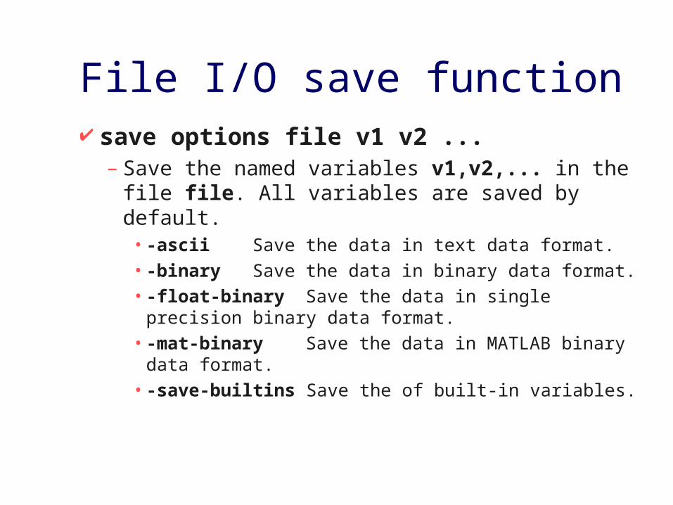
File I/O save function save options file v1 v2 ...

– Save the named variables v1,v2,... in the file file. All variables are saved by default. •-ascii Save the data in text data format. •-binary Save the data in binary data format. •-float-binary Save the data in single precision

binary data format.•-mat-binary Save the data in MATLAB binary

data format. •-save-builtins Save the of built-in variables.

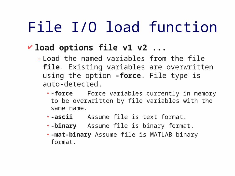
File I/O load function load options file v1 v2 ...

– Load the named variables from the file file. Existing variables are overwritten using the option -force. File type is auto-detected.•-force Force variables currently in memory to

be overwritten by file variables with the same name.•-ascii Assume file is text format. •-binary Assume file is binary format. •-mat-binary Assume file is MATLAB binary

format.

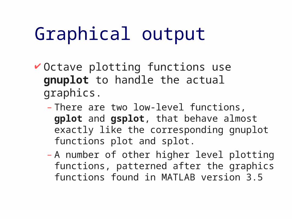
Graphical output

Octave plotting functions use gnuplot to handle the actual graphics. – There are two low-level functions, gplot and gsplot, that behave almost exactly like the corresponding gnuplot functions plot and splot.

– A number of other higher level plotting functions, patterned after the graphics functions found in MATLAB version 3.5

Two dimensional plotting The MATLAB-style two-dimensional plotting

commands are: – plot(x,y,fmt ...)– axis(limits)– hold on|off– ishold– replot– clearplot– closeplot

Three dimensional plotting

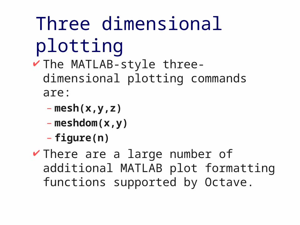
The MATLAB-style three-dimensional plotting commands are: – mesh(x,y,z)– meshdom(x,y)– figure(n)

There are a large number of additional MATLAB plot formatting functions supported by Octave.

Octave updates

GNU Octave is freely redistributable software. You may redistribute it and/or modify it under the terms of the GNU General Public License (GPL) as published by the Free Software Foundation.

Octave was written by John W. Eaton and many others. Because Octave is free software you are encouraged to help make Octave more useful by writing and contributing additional functions for it, and by reporting any problems you may have.Visit the Octave web site: http://www.che.wisc.edu/octave/octave.html