ESSENTIAL M

ATLAB®AN

D OCTAVERogel-Salazar

ISBN: 978-1-4822-3463-3

9 781482 234633

90000

K23005

Mathematics

“Essential MATLAB® and Octave is a superb introductory textbook for those interested in learning how to solve scientific, engineering, and mathematical problems using two of the most popular mathematical programming tools available. The book assumes almost no prior experience with programming or scientific programming, and carefully takes the reader step by step through the use of the two languages for solving increasingly complex problems. …Dr. Rogel-Salazar has put a huge amount of effort into making the book accessible and user friendly in a way that makes it suitable even for the most novices of programmers.” —Dr. Shashank Virmani, Brunel University London, UK

“The text provides a clear and easy-paced introduction to MATLAB® and Octave. The presentation is example led and contains plenty of useful applications drawn from mathematics, physics, and engineering. This beginner’s handbook will suit a broad scientific readership.” —Dr. Alan McCall, University of Hertfordshire, UK

Learn Two Popular Programming Languages in a Single Volume

Widely used by scientists and engineers, well-established MATLAB® and open-source Octave are similar software programs providing excellent capabilities for data analysis, visualization, and more. By means of straightforward explanations and examples from different areas in mathematics, engineering, finance, and physics, Essential MATLAB and Octave explains how MATLAB and Octave are powerful tools applicable to a variety of problems. This text provides an introduction that reveals basic structures and syntax, demonstrates the use of functions and procedures, outlines availability in various platforms, and highlights the most important elements for both programs.

Effectively Implement Models and Prototypes Using Computational Models

This text requires no prior knowledge. Self-contained, it allows the reader to use the material whenever needed rather than follow a particular order. Compatible with both languages, the book material incorporates commands and structures that allow the reader to gain a greater awareness of MATLAB and Octave, write their own code, and implement their scripts and programs within a variety of applicable fields. It is always made clear when particular examples apply only to MATLAB or only to Octave, allowing the book to be used flexibly depending on readers’ requirements.

Essential MATLAB and Octave offers an introductory course in MATLAB and Octave programming, and is a perfect resource for students in physics, mathematics, statistics, engineering, and any other subjects that require the use of computers to solve numerical problems.

K23005_COVER_final.indd 1 9/26/14 10:44 AM

ESSENTIALMATLAB®

AND OCTAVE

K23005_FM.indd 1 10/1/14 3:16 PM

K23005_FM.indd 2 10/1/14 3:16 PM

ESSENTIALMATLAB®

AND OCTAVE

Jesús Rogel-Salazar

Boca Raton London New York

CRC Press is an imprint of theTaylor & Francis Group, an informa business

K23005_FM.indd 3 10/1/14 3:16 PM

MATLAB® is a trademark of The MathWorks, Inc. and is used with permission. The MathWorks does not warrant the accuracy of the text or exercises in this book. This book’s use or discussion of MATLAB® software or related products does not constitute endorsement or sponsorship by The MathWorks of a particular pedagogical approach or particular use of the MATLAB® software.

CRC PressTaylor & Francis Group6000 Broken Sound Parkway NW, Suite 300Boca Raton, FL 33487-2742

© 2015 by Taylor & Francis Group, LLCCRC Press is an imprint of Taylor & Francis Group, an Informa business

No claim to original U.S. Government worksVersion Date: 20140930

International Standard Book Number-13: 978-1-4822-3464-0 (eBook - PDF)

This book contains information obtained from authentic and highly regarded sources. Reasonable efforts have been made to publish reliable data and information, but the author and publisher cannot assume responsibility for the validity of all materials or the consequences of their use. The authors and publishers have attempted to trace the copyright holders of all material reproduced in this publication and apologize to copyright holders if permission to publish in this form has not been obtained. If any copyright material has not been acknowledged please write and let us know so we may rectify in any future reprint.

Except as permitted under U.S. Copyright Law, no part of this book may be reprinted, reproduced, transmitted, or utilized in any form by any electronic, mechanical, or other means, now known or hereafter invented, including photocopying, microfilming, and recording, or in any information storage or retrieval system, without written permission from the publishers.

For permission to photocopy or use material electronically from this work, please access www.copyright.com (http://www.copyright.com/) or contact the Copyright Clearance Center, Inc. (CCC), 222 Rosewood Drive, Danvers, MA 01923, 978-750-8400. CCC is a not-for-profit organization that provides licenses and registration for a variety of users. For organizations that have been granted a photocopy license by the CCC, a separate system of payment has been arranged.

Trademark Notice: Product or corporate names may be trademarks or registered trademarks, and are used only for identification and explanation without intent to infringe.

Visit the Taylor & Francis Web site athttp://www.taylorandfrancis.com

and the CRC Press Web site athttp://www.crcpress.com

To A. J. Johnson

vii

Contents

1 MATLAB® and Octave: The Essential Essentials 1

1.1 MATLAB and Octave 1

1.1.1 Obtaining MATLAB 2

1.1.2 Obtaining Octave 3

1.2 Starting Up and Closing Down 3

1.2.1 Windows Systems 3

1.2.2 UNIX 4

1.2.3 Mac OS Systems 5

1.2.4 Command Line Help 6

1.2.5 Demos in MATLAB 8

1.3 Using MATLAB and Octave as a Calculator 8

1.4 Numbers and Formats 9

1.5 Variables 10

1.5.1 Variable Names 11

1.6 Suppressing Output 13

1.7 Built-In Functions 15

1.7.1 Trigonometric Functions 15

1.7.2 Other Elementary Functions 15

viii j. rogel-salazar

1.8 Characters, String and Text 17

1.8.1 Comparing Strings 20

1.8.2 Converting Strings to Values 21

1.9 Saving a Session 21

1.10 Summary 24

1.11 Exercises 25

2 Vectors and Vector Operators 27

2.1 Vectors 27

2.2 The Colon Notation (:) 32

2.3 Extracting Parts of a Vector 34

2.4 Column Vectors 37

2.5 Transposition of Vectors 38

2.6 Vector Multiplication 42

2.7 Scalar Product, * 42

2.8 Dot-Star Product, .* 46

2.9 Dot-Division of Vectors, ./ 48

2.10 Dot-Power of Vectors, .^ 50

2.11 Summary 51

2.12 Exercises 53

3 Matrices and Matrix Operators 57

3.1 Size of a Matrix 59

3.2 Transpose of a Matrix 60

essential matlab®

and octave ix

3.3 Special Matrices 62

3.3.1 Square Matrices 64

3.3.2 The Identity Matrix 65

3.4 Diagonal Matrices 67

3.5 Building Matrices 70

3.6 Tabulating Functions 73

3.7 Extracting Parts of Matrices 75

3.8 Matrix Multiplication 79

3.8.1 Dot-Star Product of Matrices, .* 80

3.8.2 Matrix-Vector Products 82

3.8.3 Matrix-Matrix Products 84

3.9 Sparse Matrices 86

3.10 Systems of Linear Equations 93

3.11 Summary 96

3.12 Exercises 98

4 Plotting 103

4.1 Plotting Simple Functions 103

4.2 Information in the Plot 107

4.2.1 Titles and Labels 108

4.2.2 Grids 108

4.2.3 Line Styles and Colours 109

x j. rogel-salazar

4.3 Multiple Plots 110

4.4 Holding Figures 111

4.5 Subplots 113

4.6 Formatted Text 115

4.7 Changing Axes 118

4.8 Plotting Surfaces 121

4.9 More Plots 125

4.9.1 Log Plots 126

4.9.2 Plots in Other Coordinate Systems 128

4.9.3 Saving Plots 130

4.10 Summary 132

4.11 Exercises 134

5 Programming MATLAB® and Octave 137

5.1 Script Files 137

5.1.1 Text Editors 138

5.1.2 Adding Comments 139

5.2 Flow of a Programme 139

5.2.1 Relational Operators 140

5.2.2 Relational Operators with Vectors and Matrices 142

5.2.3 Logical Operators 146

5.2.4 Selecting Elements with Logical Operators 148

5.3 Loops in MATLAB and Octave 153

5.3.1 For Loop 155

5.3.2 While Loop 158

essential matlab®

and octave xi

5.4 Conditionals: If... Then... Else... 161

5.5 Procedures and Functions with m-Files 164

5.5.1 Putting It All Together: m-Files 164

5.5.2 Functions in m-Files 168

5.6 Built-In Functions 172

5.6.1 Matrix and Vector Functions 173

5.6.2 Trigonometric Functions 174

5.6.3 Functions for Complex Numbers 175

5.6.4 Exponential and Logarithmic Functions 176

5.6.5 Rounding and Reminder Functions 176

5.6.6 Special Functions 177

5.6.7 Number Theoretic Functions 178

5.6.8 Coordinate Transformations 178

5.6.9 Statistics 179

5.6.10 Data Interpolation 179

5.6.11 Polynomials 180

5.6.12 Finite Differences 181

5.6.13 Differential Equations 181

5.6.14 Optimisation and Root Finding 181

5.6.15 Fourier Transforms 181

5.7 Function Handles 182

5.7.1 Anonymous Functions 183

5.7.2 Arrays of Function Handles 184

5.7.3 Function Handles as Arguments 185

xii j. rogel-salazar

5.8 Debugging 187

5.9 Timing 191

5.10 Reading and Writing Files 192

5.10.1 Formatted Files 193

5.10.2 Reading Formatted Files 193

5.10.3 Writing Formatted Files 196

5.10.4 Binary Files 198

5.10.5 Writing Binary Files 198

5.10.6 Reading Binary Files 199

5.11 Summary 200

5.12 Exercises 202

6 MATLAB® and Octave in Action 205

6.1 Linear Algebra: Linear Combinations 206

6.2 Linear Algebra: Eigenvalues and Eigenvectors 208

6.3 Portfolio Risk: Minimum Variance and Target Portfolios 212

6.3.1 Minimum Variance Portfolio 213

6.3.2 Target Portfolio 216

6.4 Differential Equations: Predator-Prey Model 219

6.4.1 Ordinary Differential Equation System in MATLAB 221

6.4.2 Ordinary Differential Equation System in Octave 222

6.4.3 Solving the Predator-Prey System 223

6.5 Signal Processing: Fourier Transform 228

6.5.1 Amplitude Spectrum 229

6.5.2 Noise Filtering 230

essential matlab®

and octave xiii

6.6 Physics: The Wave Equation 235

6.6.1 Oscillations in a String 235

6.6.2 Oscillations in a Circular Membrane 238

6.7 Quantum Mechanics: The Schrödinger Equation and Pauli Matrices 242

6.7.1 Particle in an Infinite Potential Well 242

6.7.2 Pauli Spin Matrices 245

6.8 Summary 248

6.9 Exercises 250

Differences between MATLAB® and Octave 253

Bibliography 257

Index 259

xv

List of Figures

3.1 Non-zero elements of the matrix p_new defined in the text.

The command spy can be used to obtain a visual represen-

tation of the non-zero elements of a matrix. 73

4.1 Plot of the function y = cos(4x) generated with 21 sam-

ple points. The low sampling generates a jagged profile. 106

4.2 Plot of the function y = cos(4x) generated with 200 sam-

ple points. Increasing the number of points gives us a smoother

curve. 107

4.3 Plot of the function y = cos(4x) including a title and la-

bels for each axis. 109

4.4 Multiple plots in the same figure can be placed using the

plot command. 112

4.5 Subplots can be graphed with the command subplot. Each

subplot can be given its own labels, grids, titles, etc. 115

4.6 Multiple plots in the same figure can be placed using the

plot command. 119

4.7 Graph of y = x2 for values of x between 10 and 20. The

y-axis is showing values between −2 and 500. 121

4.8 A surface plot obtained with the surfl command. Please

note that this requires the generation of a grid with the com-

mand meshgrid. 124

4.9 The projection of the surface shown in Figure 4.8. This plot

was obtained using the contour command. 126

xvi j. rogel-salazar

4.10 Comparison of the plot of the function f (x) = 4 exp(2x)in linear Cartesian coordinates (top panel) and in a semi-

logarithmic scale (bottom panel). 128

4.11 Polar plot for the function r = 2 (1 − cos(t)) as gener-

ated by MATLAB; Octave will produce a similar but sim-

pler graphic. The heart-like shape of the plot inspired the

name used for these functions: cardioids. 130

4.12 Plot for the function r = 2 (1 − cos(t)) in Cartesian co-

ordinates. The coordinate transformation was handled by

the pol2cart command. 131

5.1 Plotting functions with singularities leads to figures that

do not represent the true characteristics of the function. In

this case we are showing what happens when trying a naive

approach when plotting the tangent function y = tan(x). 153

5.2 The use of logical operators can help us improve those plots

where singularities may arise. Here we can indeed distin-

guish the important features of the tangent function y =

tan(x). 154

5.3 Output of the script called my_plot_script.m as shown in

the code described in this chapter, with frequency=1 and

whichplot=1. 167

5.4 Output of the script called my_plot_script.m. for frequency=3

and whichplot=2. 169

6.1 Solving the predator-prey model given by Equations (6.42)

and (6.43). Panel a) shows the dynamics of the predator and

prey populations, whereas panel b) shows the behaviour

in phase space. 227

6.2 Sample of the signal given by Equation (6.47) for an inter-

val of 2 seconds at a sample rate of 0.01. 229

6.3 Amplitude spectrum of the signal given by Equation (6.47).

Notice the peaks at the frequencies of 3 Hz and 4.5 Hz, with

amplitudes 3 and 8, respectively. 231

essential matlab®

and octave xvii

6.4 Panel a) Noisy signal generated by adding random noise

to original sampling. Panel b) Amplitude spectrum of the

noisy signal. 233

6.5 Corrected signal after applying a low amplitude filter to the

noisy input. 234

6.6 Initial condition for the simulation of an oscillating string. 236

6.7 Modes of a 2D circular membrane, for m=0,1 and n=1,2. 241

6.8 Eigenfunctions n=1,2,3,4 for a quantum particle confined

in an infinite potential well. 246

xix

List of Tables

1.1 Some of the types that are supported in MATLAB and Oc-

tave. 9

1.2 Some number formats used by MATLAB and Octave. 10

1.3 Some of the mathematical functions defined in MATLAB

and Octave. 16

4.1 Colours and line styles that can be used by MATLAB. 110

4.2 Some graphics formats supported by the command print. 132

5.1 Some relational operators supported by Matlab and Octave. 140

5.2 Some logical operators supported by MATLAB and Octave. 146

5.3 Permissions for opening files with fopen. 193

5.4 Format definitions for reading and writing data. 195

5.5 Control characters used in formatting output. 197

5.6 Precision specifiers for reading and writing binary data. 199

xxi

Preface

This book is an introduction to the most essential

aspects of MATLAB®1 and GNU Octave. It is intended 1 For product information pleasecontact:

The MathWorks, Inc.3 Apple Hill DriveNatick, MA 01760-2098 USATel: 508-647-7000

Fax: 508-647-7001

E-mail: info@mathworks.comWeb: www.mathworks.com

to be a companion to students in physics, mathematics,

statistics, engineering and any other subjects that require

the use of computers to solve numerical problems. The book

addresses both MATLAB and Octave with the intention of

making it easier for readers to implement their scripts and

programmes in a way that is accessible to all. On the one

hand MATLAB is a trademark of The MathWorks and as

such is a proprietary software subject to licensing. On the

other hand, GNU Octave shares many of the capabilities of

MATLAB with the added merit of being freely distributed

under the GNU General Public License.

The aim of the book is to provide straightforward explana-

tions and examples that can be readily used by readers, and

help them understand the elements of the software. The

book therefore does not provide in-depth discussions of the

implementation of specific algorithms or commands. The ex-

amples presented in this book have been tested in the latest

versions of MATLAB (R2014a) and GNU Octave (3.8). It is

important to clarify that although these two software pack-

ages share a large number of features, they are not strictly

the same and therefore care must be taken when developing

xxii j. rogel-salazar

scripts in one of them with the intention of being used in

the other. This is particularly true in the case of toolboxes

available for MATLAB that may not have a counterpart in

Octave. We assume that the reader is interacting with the

computer by issuing commands on the form of successive

lines of text (command lines). The code presented in this

book has been written with the intention of being used

in either of the packages. Throughout the text we present

computer code enclosed in a box as such:

> 1 + 1 % Example of computer code

ans =

2

We have made use of a diple (>) to denote the command

line terminal prompt in either MATLAB or Octave, and the

output is shown immediately below as it would appear in

the command line of the software itself.

In cases where the code or output is specific to MATLAB or

Octave we have added a note to that effect in the margin of

the box surrounding the command or output. For MATLAB

the box looks as follows:

MATLAB> % A margin note for code specific to MATLAB

whereas for Octave the box is shown as:

Octave> % A margin note for code specific to Octave

We have made use of margin notes, such as the one that This is an example of the marginnotes used throughout this book.appears to the right of this paragraph, to highlight certain

topics or commands, as well as to provide some useful

remarks. Please note that the output generated by MATLAB

essential matlab®

and octave xxiii

and Octave may differ in formatting and for the purposes

of the book we have decided to show a fixed number of

significant figures that fit within the boxes.

The book itself is set in a serial form where concepts in-

troduced in earlier chapters are used in later ones. Nonethe-

less, the material is sufficiently self-contained to allow the

reader to use the book as a reference tool. Having said that,

the book is intended to be more than a technical manual

and that is why we have framed examples and discussions

with a scientific twist. Furthermore, given the nature of Note that some points that arenot explicitly covered in the maintext are addressed in the Exercisessections at the end of each chapter.

programming, it is impossible to cover every single intricacy

and thus some points that are not explicitly addressed in the

text are left to the reader as further practise in the exercises.

It is important that the reader is aware that both Octave and

particularly MATLAB have a number of toolboxes available

to be used. We have not made use of these toolboxes in this

book as the main emphasis is in general programming and

scripting with both languages. Nonetheless we recommend

the reader to take a look at the Extra packages for GNU Octavesite for Octave and the Mathworks site for MATLAB.

Octave Packages available athttp://octave.sourceforge.net/

packages.php

MATLAB Toolboxes available athttp://www.mathworks.co.uk/

products/

We start Chapter 1 by introducing the software and outline

its availability in various platforms. The chapter also serves

as a foundation for the rest of the book presenting the basic

structures and syntax of the software. The book follows, in

Chapter 2, with a presentation of the simplest arrays that

MATLAB and Octave deal with: vectors. We present the

ways of manipulating the elements of a vector and show

the most common operators on vectors. We then extend the

discussion of the concept of a vector to that of a matrix in

Chapter 3. Matrices are effectively the building blocks of

the software itself. We introduce some special matrices and

explain the operations that can be done with them.

xxiv j. rogel-salazar

MATLAB and Octave have the added advantage of

incorporating a number of ready-made solutions for the

visualisation of data. Chapter 4 is dedicated to explaining

the plotting capabilities of the software as well as the for-

matting of the plots generated. In Chapter 5 we bring all

the elements discussed and explain how MATLAB and Oc-

tave are powerful programming environments. We present

the ways in which the software deals with the flow of a

programme and demonstrates the use of functions and pro-

cedures. Finally, the last chapter provides an opportunity

to see the different topics discussed earlier in the book in

use within the context of an application. We have chosen

specific examples from different areas in mathematics, en-

gineering, finance and physics and their aim is to give the

reader an idea of some of the things that can be achieved

with MATLAB and Octave rather than provide a rigorous

discussion about each subject.

The book was made possible thanks to discussions

with students and colleagues who offered suggestions for

improvement. I am very grateful for their help, in particular

to Kuldeep Singh and Alan McCall for their comments and

suggestions. I want to take this opportunity to thank my

editor at CRC Press, Francesca McGowan, whose input has

been invaluable; similarly many thanks go to the technical

reviewers whose thorough comments were more than

welcome. I would also like to express my gratitude to

my family, in particular to Antony and Bowman for their

patience and understanding throughout the writing of this

book.

London, U.K. Dr Jesús Rogel-SalazarMay 2014

xxv

About the Author

Dr Jesús Rogel-Salazar is a member of the School of

Physics, Astronomy and Mathematics at the University

of Hertfordshire, UK, and a visiting researcher at the De-

partment of Physics at Imperial College London, UK. He

obtained his doctorate in Physics at Imperial College Lon-

don for work on quantum atom optics and ultra-cold matter.

He has held a position as senior lecturer in mathematics

as well as a consultant in the financial industry since 2006.

His interests include mathematical modelling, data science

and optimisation in a wide range of applications including

optics, quantum mechanics, data journalism and finance.

1

1

MATLAB® and Octave: The Essential Essentials

The use of computers has, without a doubt, changed

the way in which science, engineering and many other

disciplines compile and analyse data. Computers provide

us with the ability of processing data at speeds that would

be impossible with pen and paper alone, and it is thus of

paramount importance to be able to instruct hardware and

software to carry out the operations we require them to

compute. This book deals with the way one can achieve

these tasks with the help of MATLAB and Octave, two very

similar numerical computing environments widely used by

scientists and engineers.

1.1 MATLAB and Octave

MATLAB stands for MATrix LABoratory and is dis-

tributed by The MathWorks1, originally created to facilitate 1 The MathWorks - http://www.mathworks.commatrix operations. It now includes capabilities to plot func-

tions and data, creation of graphical user interfaces (GUIs)

and even interaction with other programming languages

such as C++ or FORTRAN.

2 j. rogel-salazar

Octave, or to use its full name, GNU Octave2, was devel- 2 GNU Octave - http://www.octave.orgoped as a convenient command line tool for solving prob-

lems numerically in a language that is mostly compatible

with MATLAB. MATLAB is a trademark of The MathWorks

and as such is a proprietary software subject to licensing.

Conversely, GNU Octave shares many of the capabilities of

MATLAB with the added merit of being freely distributed

under the GNU General Public License. In this book we

present code that is compatible with both languages in the

expectation of enhancing the numerical computing capabili-

ties of the reader.

This book presents some of the most essential aspects of

MATLAB and Octave programming, and it is important to

mention that it is not meant to be an exhaustive manual for

either. In cases where further in-depth manual-style infor-

mation is required, the interested reader is recommended

to consult directly MATLAB manuals3,4 as well as Octave 3 Higham, D. J. and N. J. Higham(2005). MATLAB Guide. Soci-ety for Industrial and AppliedMathematics4 Palm, W. J. (2008). A ConciseIntroduction to MATLAB. McGraw-Hill Higher Education

ones5,6.

5 Hansen, J. S. (2011). GNU OctaveBeginner’s Guide. Learn by doing:less theory, more results. PacktPublishing, Limited6 Eaton, J. W., D. Bateman, andS. Hauberg (2008). GNU OctaveManual: Version 3. A GNU manual.Network Theory Limited

1.1.1 Obtaining MATLAB

MATLAB licenses can be purchased directly from

The MathWorks, which shall be able to provide further

information regarding the platforms supported as well as

the system requirements for the software. The software is

typically available for Windows, Mac OS and UNIX/Linux.

Generally speaking, the installation procedure is guided

by the software setup and a MathWorks account as well as

an activation key is required. Further information can be

obtained from www.mathworks.com.

essential matlab®

and octave 3

1.1.2 Obtaining Octave

As mentioned above, Octave is distributed under the

terms of the GNU General Public License7 and although it 7 GNU (June 29, 2007). Gen-eral Public License, Free Soft-ware Foundation, version 3.http://www.gnu.org/licenses/gpl(Last visited Aug 4,2014)

is primarily designed to run under Linux, there are imple-

mentations that run in Windows and Mac OS. The software

can be directly downloaded from http://www.octave.org

but it may be easier for the unexperienced user to download

a packaged installation file. These packages are available for

Windows and Mac OS and can be found in the Octave-Forge

website: http://octave.sourceforge.net. The installation

procedure is then guided by the package itself.

1.2 Starting Up and Closing Down

1.2.1 Windows Systems

On Windows systems MATLAB is started by double-

clicking the MATLAB icon on the desktop. This will open

up a window divided in various subwindows and at the

top the user will find the typical toolbars used in many

Windows applications. One of the subwindows shows a

command line terminal where the prompt is indicated

with >>. It is in this window where we can type various

commands to carry out calculations. To close MATLAB

simply type

> quit

in the command line or close the window as you would do

with any other application in Windows.

Octave can be launched in a very similar fashion; the main

difference is that, unlike MATLAB, the only window that

4 j. rogel-salazar

is available to the user is the command line, typically indi-

cated with octave:1>. For the purposes of this book we will

denote the command line for both MATLAB and Octave as >

only.

To close Octave you can type quit as it is done for MATLAB

or simply

Octave> exit

It may seem very daunting at first not to have the comfort

of icons around the main window provided by the Java GUI

that comes with MATLAB, but do not let this put you off.

In this chapter, as well as in the following ones, you will

familiarise yourself with the command line environment

and in no time you will master the use of MATLAB and

Octave even if the familiar-looking icons are not there.

1.2.2 UNIX

If you are a UNIX user you are probably familiar with

the idea that a number of commands are entered directly

in a terminal shell. To start MATLAB on a UNIX platform

simply type the command matlab in the shell as follows:

MATLAB> matlab

It may be the case that you will need to launch the software

in an xterm window, depending on the version of MATLAB

you are using. For further information about this please

consult The MathWorks8. 8 The MathWorks - http://www.mathworks.com

Octave can be started in the same way; in other words,

simply type the command octave at the system prompt as

follows:

essential matlab®

and octave 5

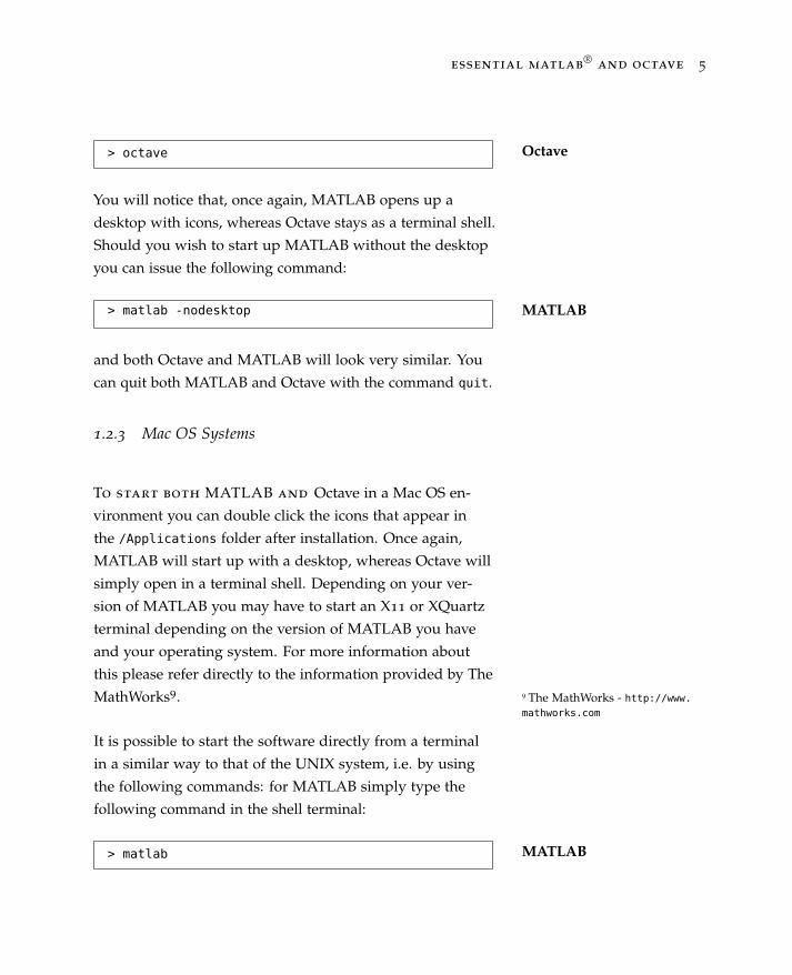
Octave> octave

You will notice that, once again, MATLAB opens up a

desktop with icons, whereas Octave stays as a terminal shell.

Should you wish to start up MATLAB without the desktop

you can issue the following command:

MATLAB> matlab -nodesktop

and both Octave and MATLAB will look very similar. You

can quit both MATLAB and Octave with the command quit.

1.2.3 Mac OS Systems

To start both MATLAB and Octave in a Mac OS en-

vironment you can double click the icons that appear in

the /Applications folder after installation. Once again,

MATLAB will start up with a desktop, whereas Octave will

simply open in a terminal shell. Depending on your ver-

sion of MATLAB you may have to start an X11 or XQuartz

terminal depending on the version of MATLAB you have

and your operating system. For more information about

this please refer directly to the information provided by The

MathWorks9. 9 The MathWorks - http://www.mathworks.com

It is possible to start the software directly from a terminal

in a similar way to that of the UNIX system, i.e. by using

the following commands: for MATLAB simply type the

following command in the shell terminal:

MATLAB> matlab

6 j. rogel-salazar

Please note that it may be necessary to modify the path in

your computer so that the command line knows where to

find the appropriate application.

In the case of Octave, the application can be started by

typing the following in the command line:

Octave> octave

Finally, to exit both MATLAB and Octave simply type quit

at the command line:

> quit

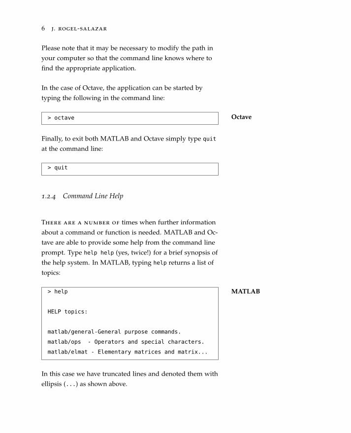
1.2.4 Command Line Help

There are a number of times when further information

about a command or function is needed. MATLAB and Oc-

tave are able to provide some help from the command line

prompt. Type help help (yes, twice!) for a brief synopsis of

the help system. In MATLAB, typing help returns a list of

topics:

MATLAB> help

HELP topics:

matlab/general-General purpose commands.

matlab/ops - Operators and special characters.

matlab/elmat - Elementary matrices and matrix...

In this case we have truncated lines and denoted them with

ellipsis (...) as shown above.

essential matlab®

and octave 7

In Octave, help explains the use of this function. We can ob-

tain help for a particular command or function by preceding

its name with the command help:

Octave> help

For help with individual commands and functions

type

help NAME

(replace NAME with the name of the command

or function you would like to learn more

about).

Let us take a look at the help for one of the built-in func-

tions in the software, namely, the function ones:

MATLAB> help ones

ONES Ones array.

ONES(N) is an N-by-N matrix of ones.

ONES(M,N) or ONES([M,N]) is an M-by-N

matrix of ones

You can do the same in Octave. For certain functions, the

information given by help can be quite lengthy. In order to

see the information one screen at a time, first turn on the

command more, i.e.,

> more on

> help ones

You can then hit any key to read on the information pro-

vided.

8 j. rogel-salazar

1.2.5 Demos in MATLAB

Demonstrations can be very useful as they provide

some examples of the capabilities of the software. MATLAB

has a number of them and they can be accessed by typing

the command demo in the command line of the programme.

Please note that this command will clear any information

that is currently in MATLAB’s workspace. Unfortunately

there is not an equivalent of this command in Octave, but

you can obtain a number of examples on the web or keep on

reading this book!

1.3 Using MATLAB and Octave as a Calculator

The basic arithmetic operators are addition +, sub-

straction −, multiplication *, division / and exponentiation

^ and these are used in conjunction with brackets: ( ).

The symbol ^ is used to get exponents (powers): for exam-

ple, 42 can be obtained with the commands 4^2=16. The

calculations can be typed directly in the command line:

> 9+2/8*6

ans =

10.5000

There could be a certain amount of ambiguity with the

calculation above. Is this 9+2/(8*6) or 9+(2/8)*6? MATLAB

works according to the following priorities:

Priorities for arithmetic calcula-tions.

1. Quantities in brackets

2. Powers (1+4^2=1+16=17)

essential matlab®

and octave 9

3. The operators * /, working left to right (2/8*6=0.25*6)

4. The operators + −, working left to right (4+6−6=10−6)

The calculation we referred to earlier on is thus for 9 + (2/8)*6,

by priority 3.

1.4 Numbers and Formats

MATLAB and Octave recognise several different

kinds of numbers, some of which are shown in Table 1.1.

Similarly, the software can display numbers in different

formats. They can be controlled with the command format

and some common formats are shown in Table 1.2.

Type Examples

Integer 2, −98765Real 5.4321, −80.768Complex 7.76 − 6.42i (i =

√−1)

Inf Infinity (result of dividing by zero)NaN Not a Number, 0/0

Table 1.1: Some of the types thatare supported in MATLAB andOctave.

The “e” notation is used for very large or very small num-

bers:

7.93796e+03 = 7.93796 × 103 = 7937.96

7.93796e− 01 = 7.93796 × 10−1 = 0.793796

All computations in MATLAB and Octave are done

in double precision, that is to say that about 15 significant

figures are used. The displayed format of the output is

handled by the command format; if the format is changed

and you want to go back to the default simply use the

command with no further input argument. A common

formatting is the one given by

10 j. rogel-salazar

format compact

which suppresses blank lines in the output and allows you a

better use of the workspace real state.

Command Example of output

format short 6.022 (4 decimal places)format short e 6.022e+23

format long e 6.0221415e+23

format bank 6.02 (2 decimal places)

Table 1.2: Some number formatsused by MATLAB and Octave.

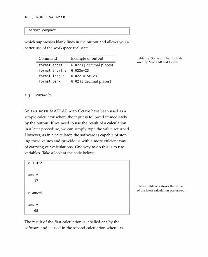
1.5 Variables

So far both MATLAB and Octave have been used as a

simple calculator where the input is followed immediately

by the output. If we need to use the result of a calculation

in a later procedure, we can simply type the value returned.

However, as in a calculator, the software is capable of stor-

ing these values and provide us with a more efficient way

of carrying out calculations. One way to do this is to use

variables. Take a look at the code below:

The variable ans stores the valueof the latest calculation performed.

> 1+4^2

ans =

17

> ans*4

ans =

68

The result of the first calculation is labelled ans by the

software and is used in the second calculation where its

essential matlab®

and octave 11

value is changed. Please note that ans will always store

the result of the latest calculation and therefore it is not

recommended to use it at length. It is preferable to create

ad hoc names to store values. In that way we can assign

the results of calculations to variables that can later be

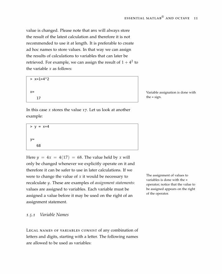
retrieved. For example, we can assign the result of 1 + 42 to

the variable x as follows:

Variable assignation is done withthe = sign.

> x=1+4^2

x=

17

In this case x stores the value 17. Let us look at another

example:

> y = x*4

y=

68

Here y = 4x = 4(17) = 68. The value held by x will

only be changed whenever we explicitly operate on it and

therefore it can be safer to use in later calculations. If we

were to change the value of x it would be necessary to

recalculate y. These are examples of assignment statements:

values are assigned to variables. Each variable must be

The assignment of values tovariables is done with the =

operator; notice that the value tobe assigned appears on the rightof the operator.assigned a value before it may be used on the right of an

assignment statement.

1.5.1 Variable Names

Legal names of variables consist of any combination of

letters and digits, starting with a letter. The following names

are allowed to be used as variables:

12 j. rogel-salazar

RateVal, Phi2y, x1, X2, z1y2, Theta_1

whereas the following names are not allowed to be used as

variable names:

Rete-Val, 2y, %x, @sign, Alpha+1

The latter are not allowed because they conflict with normal

syntax of commands used by the software. Notice that the

use of underscores (_) is allowed in the declaration of vari-

ables, but not the dash. In general, it is recommended to use

names that reflect the values that the variables represent.

Another thing to remember is that there are some special

values that are defined in the software and thus these names

should not be used as variables, as this can create conflicts

difficult to debug. One example is that of the value of π,

represented by pi=3.14159...; another one is the value for The mathematical constant π isrepresented in the software by theconstant pi.

floating point relative accuracy EPS: eps = 2.2204e−16for double precision. This number can be thought of as

The floating point relative accu-racy EPS is represented by theconstant eps.

the smallest distance between two floating point numbers

as represented by the precision of the computer used. For

example, a computer with a given floating point relative

accuracy eps cannot find a floating point number between

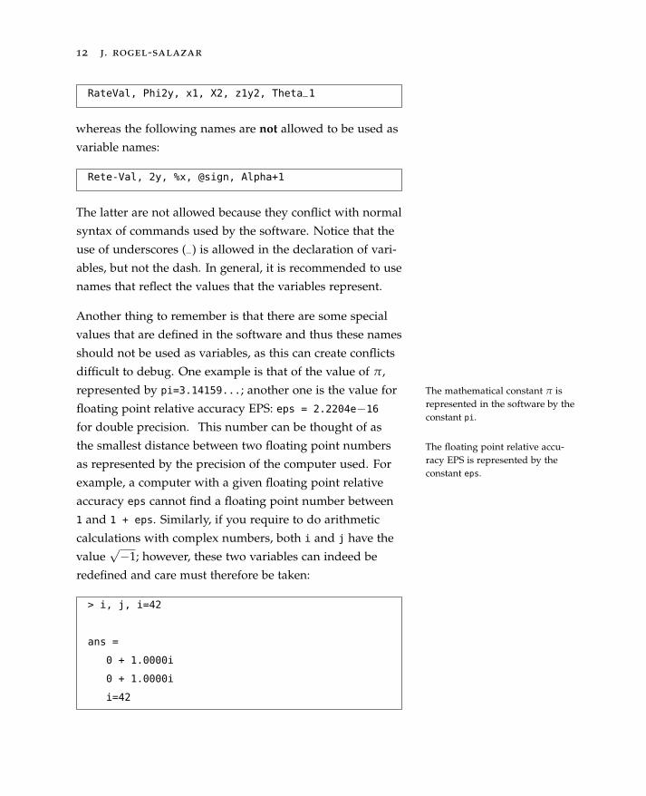
1 and 1 + eps. Similarly, if you require to do arithmetic

calculations with complex numbers, both i and j have the

value√−1; however, these two variables can indeed be

redefined and care must therefore be taken:

> i, j, i=42

ans =

0 + 1.0000i

0 + 1.0000i

i=42

essential matlab®

and octave 13

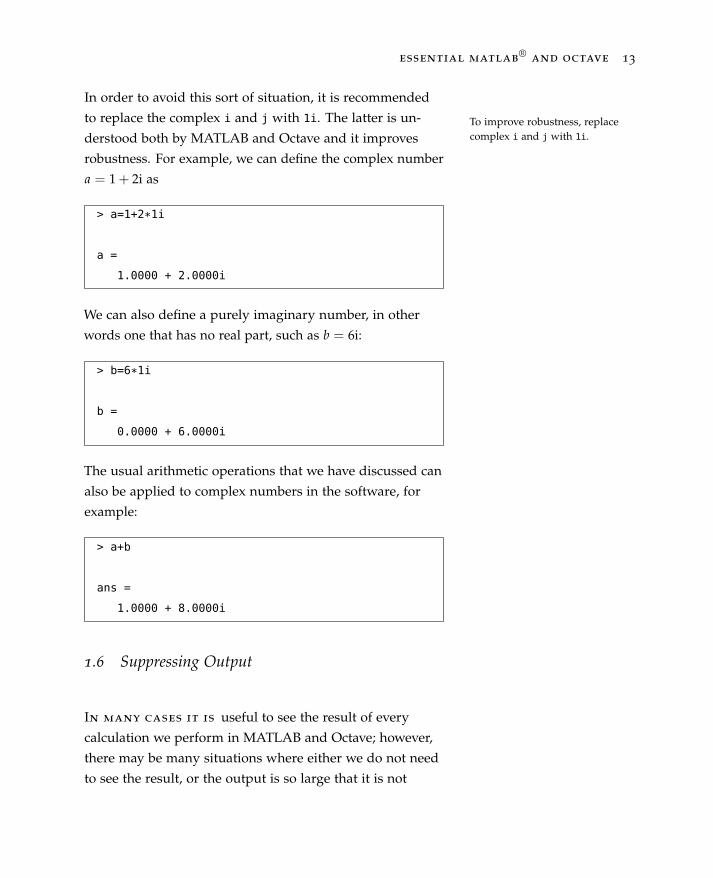
In order to avoid this sort of situation, it is recommended

to replace the complex i and j with 1i. The latter is un-

derstood both by MATLAB and Octave and it improves

robustness. For example, we can define the complex number

To improve robustness, replacecomplex i and j with 1i.

a = 1 + 2i as

> a=1+2*1i

a =

1.0000 + 2.0000i

We can also define a purely imaginary number, in other

words one that has no real part, such as b = 6i:

> b=6*1i

b =

0.0000 + 6.0000i

The usual arithmetic operations that we have discussed can

also be applied to complex numbers in the software, for

example:

> a+b

ans =

1.0000 + 8.0000i

1.6 Suppressing Output

In many cases it is useful to see the result of every

calculation we perform in MATLAB and Octave; however,

there may be many situations where either we do not need

to see the result, or the output is so large that it is not

14 j. rogel-salazar

practical to display it. In those cases, we can suppress the

output of commands by appending a semicolon (;) at the

end of the command. For instance, issuing the commandUse a semicolon (;) to avoiddisplaying output.

> x=-5

x =

-5

tells the software to display the result of the operation, in

this case echoing the assignment of −5 to the variable x.

Let us contrast this behaviour with the use of the semicolon

at the end of the line to suppress the output. Imagine that

we have a parameter x for which the value is known and

thus we do not need to display it. However, we are inter-

ested to know the output of calculations made with that

parameter. For example:

> x=-5; y = 9*x, z = x^3+y

y =

-45

z =

-170

In the code above we have suppressed the displaying of

x, however since the other commands are separated by a

comma (,) and nothing at the end of the line, the values of yand z are displayed.

essential matlab®

and octave 15

1.7 Built-In Functions

1.7.1 Trigonometric Functions

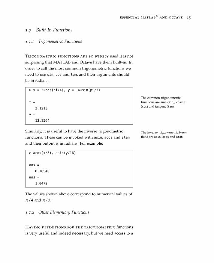
Trigonometric functions are so widely used it is not

surprising that MATLAB and Octave have them built-in. In

order to call the most common trigonometric functions we

need to use sin, cos and tan, and their arguments should

be in radians.

The common trigonometricfunctions are sine (sin), cosine(cos) and tangent (tan).

> x = 3*cos(pi/4), y = 16*sin(pi/3)

x =

2.1213

y =

13.8564

Similarly, it is useful to have the inverse trigonometric

functions. These can be invoked with asin, acos and atan

and their output is in radians. For example:

The inverse trigonometric func-tions are asin, acos and atan.

> acos(x/3), asin(y/16)

ans =

0.78540

ans =

1.0472

The values shown above correspond to numerical values of

π/4 and π/3.

1.7.2 Other Elementary Functions

Having definitions for the trigonometric functions

is very useful and indeed necessary, but we need access to a

16 j. rogel-salazar

wider range of functions and procedures. Some may include

functions such as the square root, the exponential function

and the logarithm.

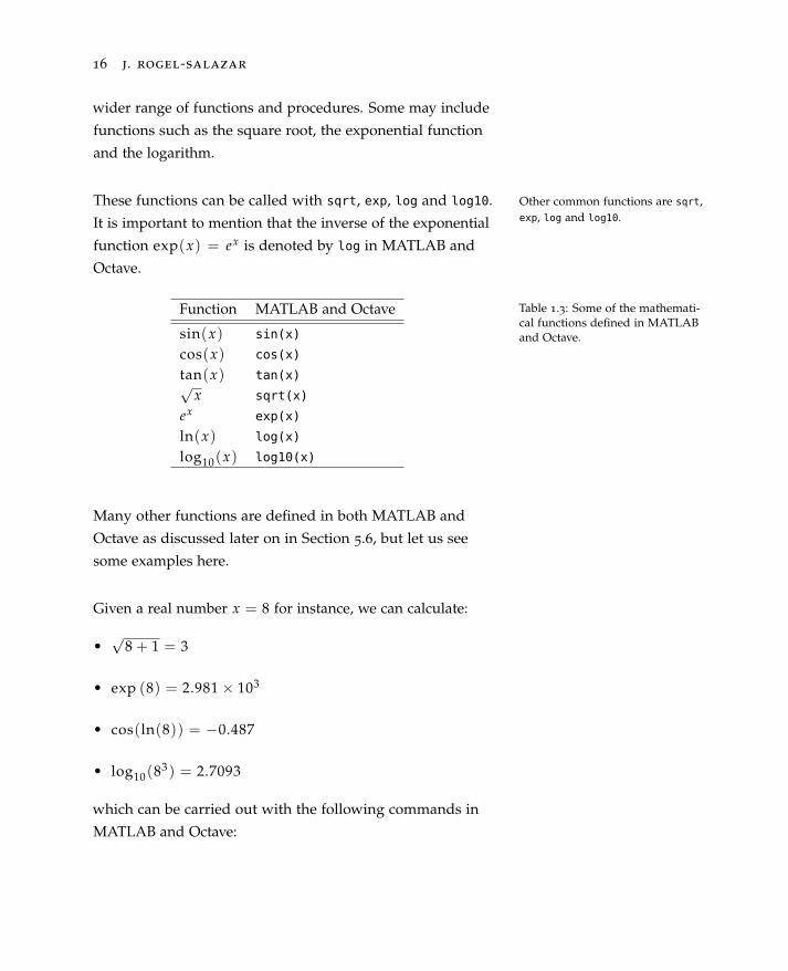
These functions can be called with sqrt, exp, log and log10. Other common functions are sqrt,exp, log and log10.It is important to mention that the inverse of the exponential

function exp(x) = ex is denoted by log in MATLAB and

Octave.

Function MATLAB and Octave

sin(x) sin(x)

cos(x) cos(x)

tan(x) tan(x)√x sqrt(x)

ex exp(x)

ln(x) log(x)

log10(x) log10(x)

Table 1.3: Some of the mathemati-cal functions defined in MATLABand Octave.

Many other functions are defined in both MATLAB and

Octave as discussed later on in Section 5.6, but let us see

some examples here.

Given a real number x = 8 for instance, we can calculate:

•√

8 + 1 = 3

• exp (8) = 2.981 × 103

• cos(ln(8)) = −0.487

• log10(83) = 2.7093

which can be carried out with the following commands in

MATLAB and Octave:

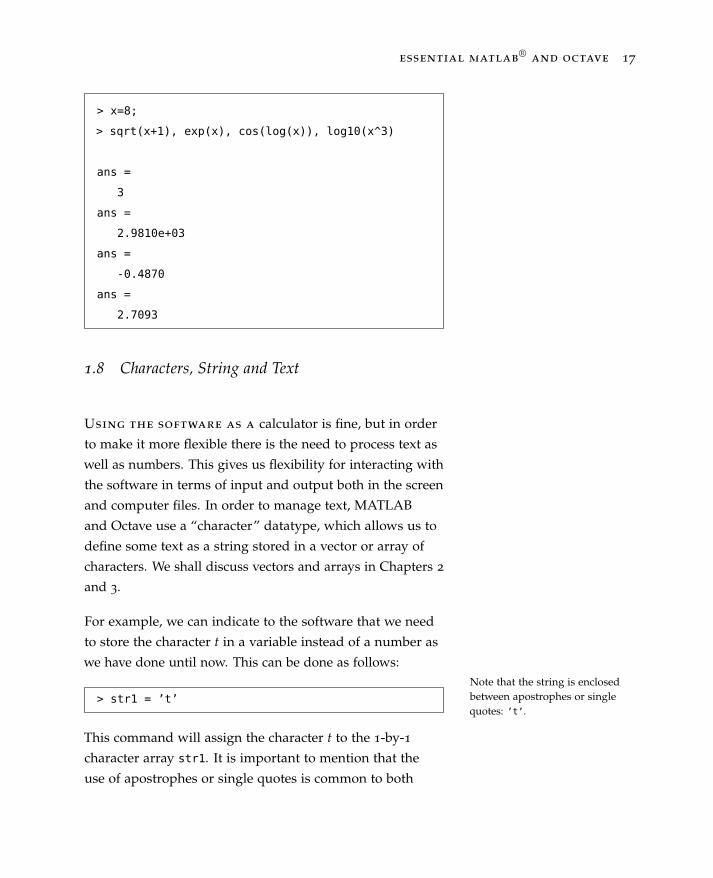
essential matlab®

and octave 17

> x=8;

> sqrt(x+1), exp(x), cos(log(x)), log10(x^3)

ans =

3

ans =

2.9810e+03

ans =

-0.4870

ans =

2.7093

1.8 Characters, String and Text

Using the software as a calculator is fine, but in order

to make it more flexible there is the need to process text as

well as numbers. This gives us flexibility for interacting with

the software in terms of input and output both in the screen

and computer files. In order to manage text, MATLAB

and Octave use a “character” datatype, which allows us to

define some text as a string stored in a vector or array of

characters. We shall discuss vectors and arrays in Chapters 2

and 3.

For example, we can indicate to the software that we need

to store the character t in a variable instead of a number as

we have done until now. This can be done as follows:Note that the string is enclosedbetween apostrophes or singlequotes: ’t’.

> str1 = ’t’

This command will assign the character t to the 1-by-1

character array str1. It is important to mention that the

use of apostrophes or single quotes is common to both

18 j. rogel-salazar

MATLAB and Octave and thus we encourage this use to

improve the portability of code between both languages.

Nonetheless, it may be useful to know that Octave also

supports the use of quotation marks to define strings. In

this case the following command is valid in Octave:

Octave supports the use of quota-tion marks to define strings.

Octave> str = ‘‘t’’

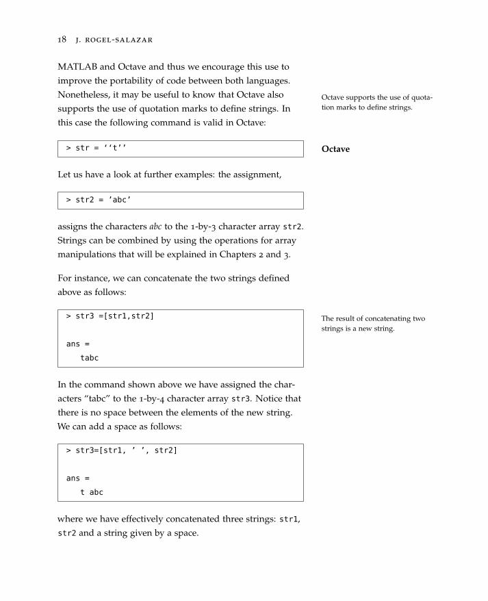
Let us have a look at further examples: the assignment,

> str2 = ’abc’

assigns the characters abc to the 1-by-3 character array str2.

Strings can be combined by using the operations for array

manipulations that will be explained in Chapters 2 and 3.

For instance, we can concatenate the two strings defined

above as follows:

The result of concatenating twostrings is a new string.

> str3 =[str1,str2]

ans =

tabc

In the command shown above we have assigned the char-

acters “tabc” to the 1-by-4 character array str3. Notice that

there is no space between the elements of the new string.

We can add a space as follows:

> str3=[str1, ’ ’, str2]

ans =

t abc

where we have effectively concatenated three strings: str1,

str2 and a string given by a space.

essential matlab®

and octave 19

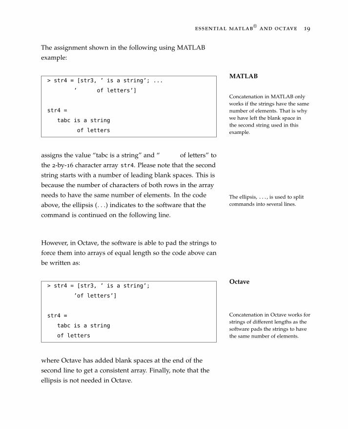
The assignment shown in the following using MATLAB

example:

MATLAB> str4 = [str3, ’ is a string’; ...

’ of letters’]

str4 =

tabc is a string

of letters

assigns the value “tabc is a string” and “ of letters” to

Concatenation in MATLAB onlyworks if the strings have the samenumber of elements. That is whywe have left the blank space inthe second string used in thisexample.

the 2-by-16 character array str4. Please note that the second

string starts with a number of leading blank spaces. This is

because the number of characters of both rows in the array

needs to have the same number of elements. In the code

above, the ellipsis (. . .) indicates to the software that the

command is continued on the following line.

The ellipsis, ..., is used to splitcommands into several lines.

However, in Octave, the software is able to pad the strings to

force them into arrays of equal length so the code above can

be written as:

Octave> str4 = [str3, ’ is a string’;

’of letters’]

str4 =

tabc is a string

of letters

where Octave has added blank spaces at the end of the

Concatenation in Octave works forstrings of different lengths as thesoftware pads the strings to havethe same number of elements.

second line to get a consistent array. Finally, note that the

ellipsis is not needed in Octave.

20 j. rogel-salazar

1.8.1 Comparing Strings

We are familiar with the idea of comparing numbers

to decide if one is larger, smaller or equal to another. In the

case of strings, we can think of checking if two strings are

equal, for example, if a script requires the user to type an

answer such as ’Continue’ or ’Stop’.

This can be achieved with the help of the strcmp command

that takes as input two strings (or variables of string type)

separated by a comma. Two strings are considered to be We can compare two strings withthe help of the strcmp command.equal if they have the same length and the content is the

same, including the case in which the strings are written.

Let us take a look at an example: If we compare the strings

’Continue’ and ’Stop’ the result is false as they do not have

the same length or content. This is denoted as a zero (0) in

MATLAB and Octave:

> s1=’Continue’

> s2=’Stop’

> strcmp(s1,s2)

ans =

0

Nonetheless, if we compare a string s1 that contains the

word Continue with the string ’Continue’ the result is true,

denoted as a one (1):

> strcmp(s1,’Continue’)

ans =

1

essential matlab®

and octave 21

1.8.2 Converting Strings to Values

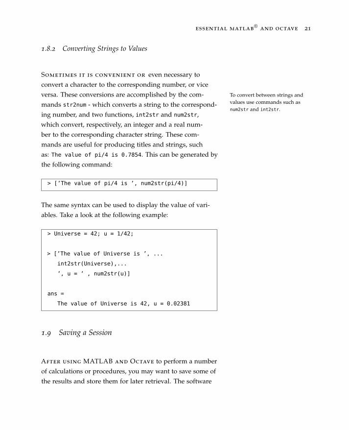
Sometimes it is convenient or even necessary to

convert a character to the corresponding number, or vice

versa. These conversions are accomplished by the com- To convert between strings andvalues use commands such asnum2str and int2str.

mands str2num - which converts a string to the correspond-

ing number, and two functions, int2str and num2str,

which convert, respectively, an integer and a real num-

ber to the corresponding character string. These com-

mands are useful for producing titles and strings, such

as: The value of pi/4 is 0.7854. This can be generated by

the following command:

> [’The value of pi/4 is ’, num2str(pi/4)]

The same syntax can be used to display the value of vari-

ables. Take a look at the following example:

> Universe = 42; u = 1/42;

> [’The value of Universe is ’, ...

int2str(Universe),...

’, u = ’ , num2str(u)]

ans =

The value of Universe is 42, u = 0.02381

1.9 Saving a Session

After using MATLAB and Octave to perform a number

of calculations or procedures, you may want to save some of

the results and store them for later retrieval. The software

22 j. rogel-salazar

allows us to save the variables that are in the memory into a

file; this can be done as follows:

> save filename.matUse save to save the variables inyour workspace to a file.

This will save the current values of all variables to a file

called filename.mat; it is a good practice to use a name for In MATLAB it is possible to leavethe extension .mat out from thesave command. It is howeverexpected by Octave.

the file that provides some useful information regarding

its contents. It is important to note that the file that is gen-

erated in this way can only be read and edited by either

MATLAB or Octave. If you need to store the information

in a formatted text file or in a binary file, please refer to

Section 5.10.

Once we have saved the file as mentioned above, we can

retrieve the information as follows:

> load filename

This command instructs MATLAB and Octave to bring up

Use the command load to retrievea saved session.

the variables and values that are stored in the file called

filename.mat; once this is done we can use and modify

their values.

Sometimes it is very useful to check the existing vari-

ables in a workspace and list their names and sizes as well

as the amount of memory they take and the class they be-

long to. This can easily be done with the whos command:

> whos

The command whos displays theexisting variables in the currentworkspace.

essential matlab®

and octave 23

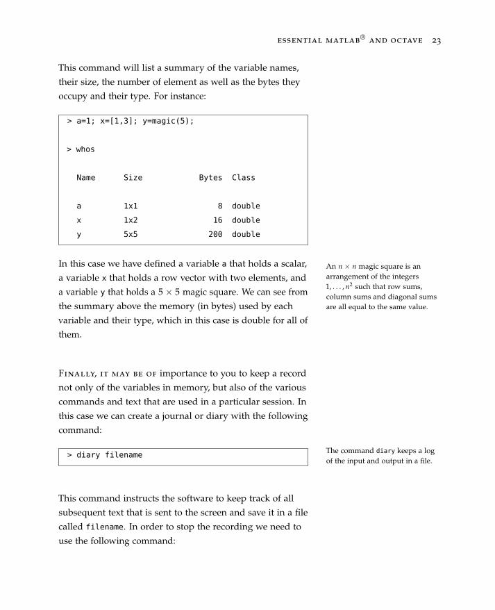
This command will list a summary of the variable names,

their size, the number of element as well as the bytes they

occupy and their type. For instance:

> a=1; x=[1,3]; y=magic(5);

> whos

Name Size Bytes Class

a 1x1 8 double

x 1x2 16 double

y 5x5 200 double

In this case we have defined a variable a that holds a scalar,

a variable x that holds a row vector with two elements, and

a variable y that holds a 5 × 5 magic square. We can see from

An n × n magic square is anarrangement of the integers1, . . . , n2 such that row sums,column sums and diagonal sumsare all equal to the same value.the summary above the memory (in bytes) used by each

variable and their type, which in this case is double for all of

them.

Finally, it may be of importance to you to keep a record

not only of the variables in memory, but also of the various

commands and text that are used in a particular session. In

this case we can create a journal or diary with the following

command:

> diary filename The command diary keeps a logof the input and output in a file.

This command instructs the software to keep track of all

subsequent text that is sent to the screen and save it in a file

called filename. In order to stop the recording we need to

use the following command:

24 j. rogel-salazar

> diary off

1.10 Summary

In this chapter we have presented an overview of what

MATLAB and Octave are, as well as general guidelines on

how to obtain the software and how to start a session in

each of them.

We have covered some useful commands (such as help

and save and whos) as well as some general features of the

software environment. We are now able to understand the

format in which numbers are presented as well as define

variables to store the output of calculations. Similarly, we

have introduced some common built-in functions such as

sin, cos, tan, log and exp.

We have seen how MATLAB and Octave are capable of

dealing with various types of numbers including integers,

decimals and complex numbers. In this way, MATLAB and

Octave can be used in the same way as a calculator. In the

next chapter we will see how the software can be used to

define vectors and how to operate with them.

essential matlab®

and octave 25

1.11 Exercises

1. MATLAB and Octave have a built-in function called clc.

Request the software for help and information about this

function.

2. Using the command-line in MATLAB and Octave, calcu-

late the following expressions:

(a) 8.23−62√

2+ 10 (3π)

(b) 9(

3√

4) ( 0.856

3)

(c) 5.3(

42(1.28)) ( 1√

(1−0.82 )(1+0.82 )

)3. Find out what the following functions do:

(a) sind

(b) cosd

(c) tand

4. Using MATLAB and Octave, calculate the value of the

following expressions:

(a) sin(3.5π)cos(1.8π)

+ 12 cot(2.1π)

(b) 6 sin (75◦) + 14 cos (63◦)

(c) log10(4987) + ln(6.5) − tan(4.1π)

5. Consider the following strings and identify which ones

are valid names for variables in MATLAB and Octave:

(a) First_One

(b) velocity 1

(c) sin

(d) myv@riable

(e) MyCalculation

(f) Last-place

26 j. rogel-salazar

(g) whichOne

(h) i

6. If t = 10, a = 9.5 − 5i, f = exp(0.1) and b = −7.356,

what are the values of the following expressions? Use

MATLAB and Octave to calculate the answers:

(a) q = t2 + b

(b) w = f − bt

(c) e = a3 − f

(d) r = f −t + 6a

7. For the evaluations carried out in Exercise 6, create

strings that display their value using the following mes-

sage:

The value of expression is value,

where expression is each of the expressions in Exercise 6

and value is the calculated result.

8. Use the number format commands in MATLAB and

Octave to display the following calculations using the

default number of decimal places, 15 decimal places and

in scientific notation:

(a) 47 + 5.13

(b) exp(0.3) − 18.1

(c) sin( 3π

7)

9. Write a series of commands that enable you to find the

roots of a quadratic equation ax2 + bx + c = 0. Set up the

commands to solve for a = 3, b = 5 and c = −6.

10. What does the built-in function clear do?

27

2

Vectors and Vector Operators

In Chapter 1 we covered some of the most basic aspects

of MATLAB® and Octave, and have seen how the software

can be used as a simple calculator to do arithmetics, as well

as performing operations using built-in functions. Nonethe-

less, both MATLAB and Octave are far more powerful than

that, and to unlock this power it is important to familiarise

ourselves with the objects that the software is able to manip-

ulate. In this chapter we will see how to deal with vectors

and the type of operations we can do with them.

2.1 Vectors

For the purposes of using MATLAB and Octave, we

can think of a vector as an arrangement of elements in a

column or a row. In that manner, vectors are effectively lists

of numbers for example, separated by either commas or

spaces. The number of entries is known as the “length” of

the vector and the entries are often referred to as “elements”

or “components” of the vector. The entries must be enclosed

28 j. rogel-salazar

in square brackets. For example, to enter the vector

vector1 =(

3, 42,√

25)

(2.1)

into MATLAB and Octave we type the following in the

command line:

Use square brackets to define avector.

> vector1 = [3 42, sqrt(25)]

vector1 =

3 42 5

In the example above we have left a space between the first

element (with value 3) and second one (with value 42). We The number of elements in avector can be separated with ablank space or with a comma (,).

could have done this explicitly with a comma, as shown in

the separation of the second (42) and third (√

25) elements.

We must be careful with the use of spaces as they can

change the number of elements in a vector and their value.

Let us have a look at the following example:

> vector2 = [8+9 5-4]

vector2 =

17 1

> vector3 = [8+9 5 -4]

vector3 =

17 5 -4

In the first line we have defined a row vector, vector2, with

Be careful when using blankspaces to define vectors; they canchange the number of elementsand their value.

two elements, but the extra space in the assignment of

vector3 creates a row vector with three elements instead.

essential matlab®

and octave 29

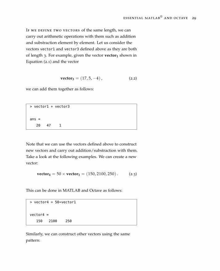
If we define two vectors of the same length, we can

carry out arithmetic operations with them such as addition

and substraction element by element. Let us consider the

vectors vector1 and vector3 defined above as they are both

of length 3. For example, given the vector vector1 shown in

Equation (2.1) and the vector

vector3 = (17, 5,−4) , (2.2)

we can add them together as follows:

> vector1 + vector3

ans =

20 47 1

Note that we can use the vectors defined above to construct

new vectors and carry out addition/substraction with them.

Take a look at the following examples. We can create a new

vector:

vector4 = 50 × vector1 = (150, 2100, 250) . (2.3)

This can be done in MATLAB and Octave as follows:

> vector4 = 50*vector1

vector4 =

150 2100 250

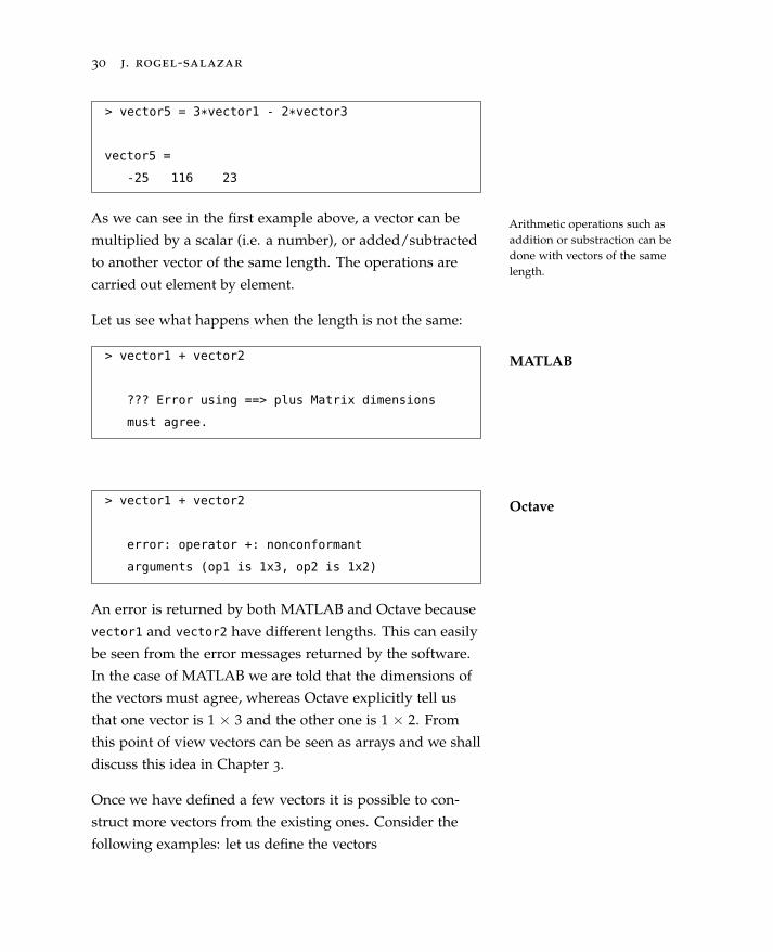
Similarly, we can construct other vectors using the same

pattern:

30 j. rogel-salazar

> vector5 = 3*vector1 - 2*vector3

vector5 =

-25 116 23

As we can see in the first example above, a vector can be

multiplied by a scalar (i.e. a number), or added/subtracted

to another vector of the same length. The operations are

carried out element by element.

Arithmetic operations such asaddition or substraction can bedone with vectors of the samelength.

Let us see what happens when the length is not the same:

MATLAB> vector1 + vector2

??? Error using ==> plus Matrix dimensions

must agree.

Octave> vector1 + vector2

error: operator +: nonconformant

arguments (op1 is 1x3, op2 is 1x2)

An error is returned by both MATLAB and Octave because

vector1 and vector2 have different lengths. This can easily

be seen from the error messages returned by the software.

In the case of MATLAB we are told that the dimensions of

the vectors must agree, whereas Octave explicitly tell us

that one vector is 1 × 3 and the other one is 1 × 2. From

this point of view vectors can be seen as arrays and we shall

discuss this idea in Chapter 3.

Once we have defined a few vectors it is possible to con-

struct more vectors from the existing ones. Consider the

following examples: let us define the vectors

essential matlab®

and octave 31

v1 = (9, 8, 7) , (2.4)

v2 = (6, 5) . (2.5)

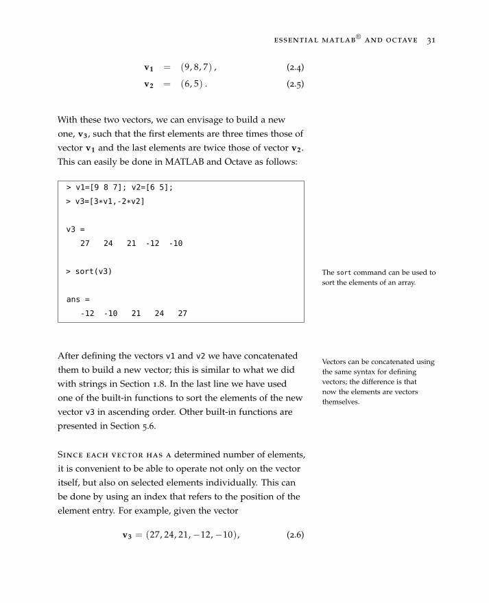
With these two vectors, we can envisage to build a new

one, v3 , such that the first elements are three times those of

vector v1 and the last elements are twice those of vector v2 .

This can easily be done in MATLAB and Octave as follows:

> v1=[9 8 7]; v2=[6 5];

> v3=[3*v1,-2*v2]

v3 =

27 24 21 -12 -10

> sort(v3)

ans =

-12 -10 21 24 27

The sort command can be used tosort the elements of an array.

After defining the vectors v1 and v2 we have concatenated

them to build a new vector; this is similar to what we did

with strings in Section 1.8. In the last line we have used

one of the built-in functions to sort the elements of the new

vector v3 in ascending order. Other built-in functions are

presented in Section 5.6.

Vectors can be concatenated usingthe same syntax for definingvectors; the difference is thatnow the elements are vectorsthemselves.

Since each vector has a determined number of elements,

it is convenient to be able to operate not only on the vector

itself, but also on selected elements individually. This can

be done by using an index that refers to the position of the

element entry. For example, given the vector

v3 = (27, 24, 21,−12,−10), (2.6)

32 j. rogel-salazar

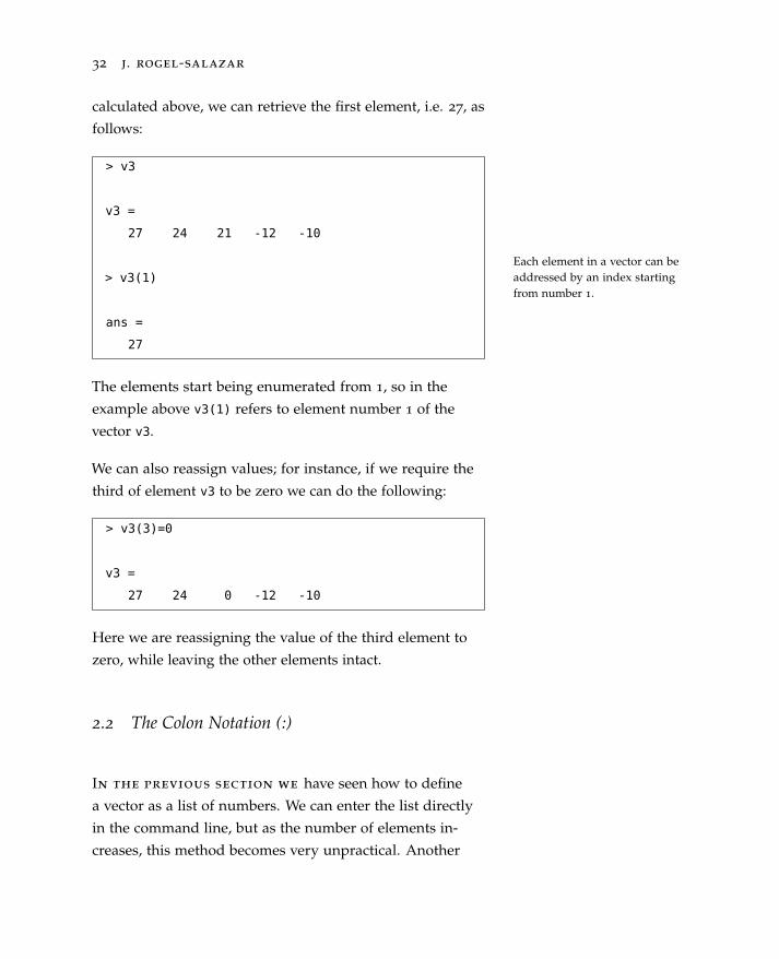
calculated above, we can retrieve the first element, i.e. 27, as

follows:

Each element in a vector can beaddressed by an index startingfrom number 1.

> v3

v3 =

27 24 21 -12 -10

> v3(1)

ans =

27

The elements start being enumerated from 1, so in the

example above v3(1) refers to element number 1 of the

vector v3.

We can also reassign values; for instance, if we require the

third of element v3 to be zero we can do the following:

> v3(3)=0

v3 =

27 24 0 -12 -10

Here we are reassigning the value of the third element to

zero, while leaving the other elements intact.

2.2 The Colon Notation (:)

In the previous section we have seen how to define

a vector as a list of numbers. We can enter the list directly

in the command line, but as the number of elements in-

creases, this method becomes very unpractical. Another

essential matlab®

and octave 33

way of defining a vector is by using a colon (:) to spec-

ify the beginning and ending elements of the vector as

beginning:ending. This will instruct the software to create

a vector that starts with beginning, and adds 1 successively

until ending (but not beyond) is reached:

The colon notation allows us todefine vectors by specifying a startand an end as beginning:ending.

> [3:9.6]

ans =

3 4 5 6 7 8 9

> [2:7]

ans =

2 3 4 5 6 7

In the first line we have asked the software to list numbers

starting with 3 and ending with 9.6. Remember that the se-

quence cannot go beyond ending. In this case the sequence

is truncated at 9. In the second example above we are listing

numbers starting with 2 and finishing with 7. In this case

the sequence reaches the ending point and no truncation is

needed.

If we try to create a series where the ending cannot be

reached by adding 1 successively an empty vector will be

returned. This is the case, for instance, when ending is

smaller than beginning. In the case of MATLAB we obtain

the following error message:

MATLAB> [2:1]

ans =

Empty matrix: 1-by-0

34 j. rogel-salazar

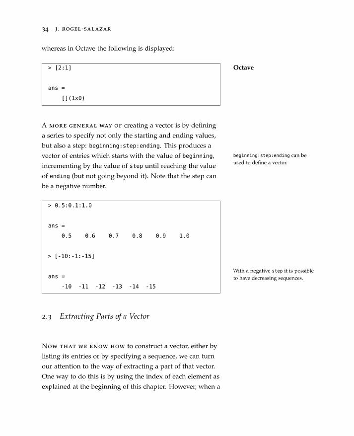
whereas in Octave the following is displayed:

Octave> [2:1]

ans =

[](1x0)

A more general way of creating a vector is by defining

a series to specify not only the starting and ending values,

but also a step: beginning:step:ending. This produces abeginning:step:ending can beused to define a vector.

vector of entries which starts with the value of beginning,

incrementing by the value of step until reaching the value

of ending (but not going beyond it). Note that the step can

be a negative number.

With a negative step it is possibleto have decreasing sequences.

> 0.5:0.1:1.0

ans =

0.5 0.6 0.7 0.8 0.9 1.0

> [-10:-1:-15]

ans =

-10 -11 -12 -13 -14 -15

2.3 Extracting Parts of a Vector

Now that we know how to construct a vector, either by

listing its entries or by specifying a sequence, we can turn

our attention to the way of extracting a part of that vector.

One way to do this is by using the index of each element as

explained at the beginning of this chapter. However, when a

essential matlab®

and octave 35

large number of elements are involved that method may not

be practical.

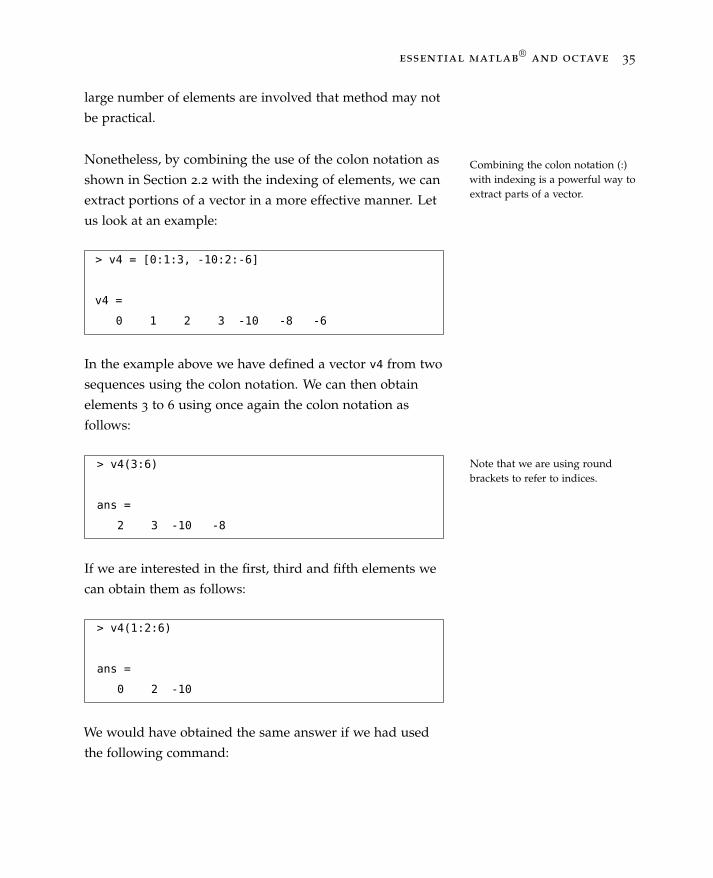
Nonetheless, by combining the use of the colon notation as

shown in Section 2.2 with the indexing of elements, we can

extract portions of a vector in a more effective manner. Let

us look at an example:

Combining the colon notation (:)with indexing is a powerful way toextract parts of a vector.

> v4 = [0:1:3, -10:2:-6]

v4 =

0 1 2 3 -10 -8 -6

In the example above we have defined a vector v4 from two

sequences using the colon notation. We can then obtain

elements 3 to 6 using once again the colon notation as

follows:

Note that we are using roundbrackets to refer to indices.

> v4(3:6)

ans =

2 3 -10 -8

If we are interested in the first, third and fifth elements we

can obtain them as follows:

> v4(1:2:6)

ans =

0 2 -10

We would have obtained the same answer if we had used

the following command:

36 j. rogel-salazar

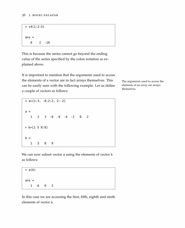
> v4(1:2:5)

ans =

0 2 -10

This is because the series cannot go beyond the ending

value of the series specified by the colon notation as ex-

plained above.

It is important to mention that the arguments used to access

the elements of a vector are in fact arrays themselves. This

can be easily seen with the following example. Let us define

a couple of vectors as follows:

The arguments used to access theelements of an array are arraysthemselves.

> a=[1:3, -8:2:2, 2:-2]

a =

1 2 3 -8 -6 -4 -2 0 2

> b=[1 5 8:9]

b =

1 5 8 9

We can now subset vector a using the elements of vector b

as follows:

> a(b)

ans =

1 -6 0 2

In this case we are accessing the first, fifth, eighth and ninth

elements of vector a.

essential matlab®

and octave 37

2.4 Column Vectors

The vectors used in the previous section are called rowvectors because the software accommodates the elements one

by one in a row. In this section we will see how to instruct

the software to define a column vector, i.e. a vector whose

entries are aligned in a column. A column vector requires

Row vectors organise the elementsin a row. Column vectors areorganised in separate lines, i.e.columns.

a new line to be inserted after each element; we achieve

this simply by separating the elements with a semicolon (;).

Consider the vector

cvector1 =

3

42√25

. (2.7)

We can enter this in the software by typing the following in

the command line:

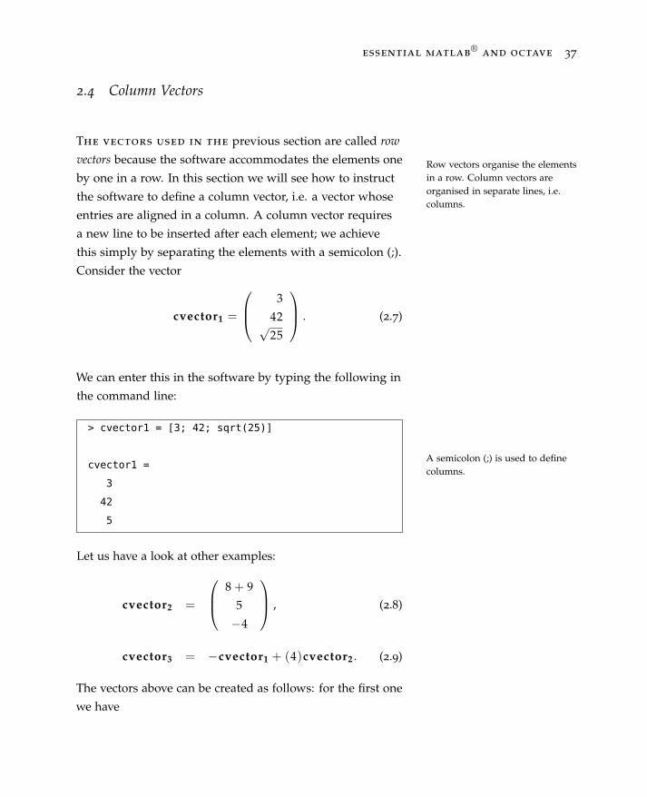
A semicolon (;) is used to definecolumns.

> cvector1 = [3; 42; sqrt(25)]

cvector1 =

3

42

5

Let us have a look at other examples:

cvector2 =

8 + 9

5

−4

, (2.8)

cvector3 = −cvector1 + (4)cvector2 . (2.9)

The vectors above can be created as follows: for the first one

we have

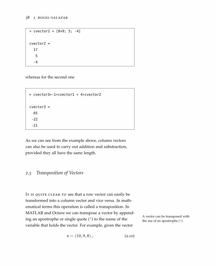
38 j. rogel-salazar

> cvector2 = [8+9; 5; -4]

cvector2 =

17

5

-4

whereas for the second one

> cvector3=-1*cvector1 + 4*cvector2

cvector3 =

65

-22

-21

As we can see from the example above, column vectors

can also be used to carry out addition and substraction,

provided they all have the same length.

2.5 Transposition of Vectors

It is quite clear to see that a row vector can easily be

transformed into a column vector and vice versa. In math-

ematical terms this operation is called a transposition. In

MATLAB and Octave we can transpose a vector by append-

ing an apostrophe or single quote (’) to the name of the

variable that holds the vector. For example, given the vector

A vector can be transposed withthe use of an apostrophe (’).

r = (10, 9, 8) , (2.10)

essential matlab®

and octave 39

its transpose would be given by

rT =

10

9

8

. (2.11)

This can be calculated in MATLAB and Octave as follows:

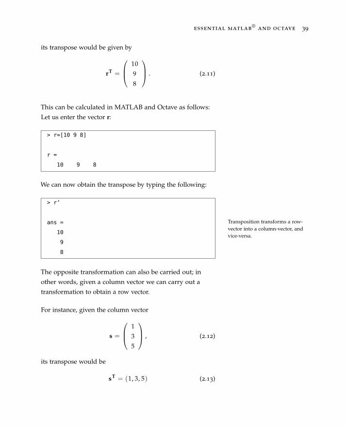
Let us enter the vector r:

> r=[10 9 8]

r =

10 9 8

We can now obtain the transpose by typing the following:

Transposition transforms a row-vector into a column-vector, andvice-versa.

> r’

ans =

10

9

8

The opposite transformation can also be carried out; in

other words, given a column vector we can carry out a

transformation to obtain a row vector.

For instance, given the column vector

s =

1

3

5

, (2.12)

its transpose would be

sT = (1, 3, 5) (2.13)

40 j. rogel-salazar

and in MATLAB and Octave this can be obtained as follows:

> s=[1; 3; 5], s’

s =

1

3

5

ans =

1 3 5

In the examples above we started out defining a row vector

r which is then easily converted into a column vector by

appending the apostrophe to the variable name, i.e. r’.

Similarly, the column vector s is transposed by typing s’.

As we have seen above, if we want to carry out addition and

substraction with vectors they need to have the same length.

They also need to be of the same kind, in other words they

all need to be either column or row vectors. Let us have a

look at an example; in MATLAB if we tried to add 3 times

the row vector r to 4 times the column vector s defined

above we would obtain the following output:

MATLAB> new_vector1 = 3*r + 4*s

??? Error using ==> plus

Matrix dimensions must agree

However, Octave broadcasts vectors, matrices and arrays until Octave is able to broadcast, i.e.repeat, a smaller vector to a largerone to carry out computations.

the objects have compatible size in order for the operation

to be valid and the software issues a warning in this regard.

essential matlab®

and octave 41

So the operation above would result in the following output

from Octave:

Octave> new_vector1 = 3*r + 4*s

warning: operator +: automatic broadcasting ...

operation applied

ans =

34 31 28

42 39 36

50 47 44

In versions of Octave prior to 3.6.0 the behaviour was simi-

lar to that of MATLAB:

Octave> new_vector1 = 3*r + 4*s

error: operator +:

nonconformant arguments (op1 is 1x3, op2 is...

3x1)

We get an error because, although the vectors do have the

same length, they are not of the same kind, i.e. one is a row

vector whereas the other one is a column vector. In order for

the above operation to return a correct answer we need to

transpose one of the vectors. We can, for instance, transpose

Some arithmetic operations (+ or−) require the vectors to be of thesame kind.

vector s and therefore the final result is stored in a row

vector,

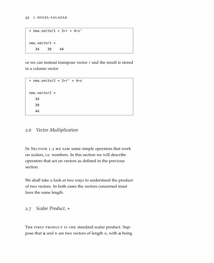
42 j. rogel-salazar

> new_vector1 = 3*r + 4*s’

new_vector1 =

34 39 44

or we can instead transpose vector r and the result is stored

in a column vector

> new_vector2 = 3*r’ + 4*s

new_vector2 =

34

39

44

2.6 Vector Multiplication

In Section 1.3 we saw some simple operators that work

on scalars, i.e. numbers. In this section we will describe

operators that act on vectors as defined in the previous

section.

We shall take a look at two ways to understand the product

of two vectors. In both cases the vectors concerned must

have the same length.

2.7 Scalar Product, *

The first product is the standard scalar product. Sup-

pose that u and v are two vectors of length n, with u being

essential matlab®

and octave 43

a row vector and v a column vector:

u = (u1 , u2 , . . . , un) , (2.14)

v =

v1

v2...

vn

. (2.15)

The scalar product is defined by multiplying the correspond-

ing elements together and adding the results to give a single

number, i.e. a scalar:

Definition of the scalar product.u ∗ v =n

∑i=1

ui vi , (2.16)

where we have used the symbol ∗ to denote the operation

(this indeed is the symbol used by MATLAB and Octave for

the scalar product).

For example, let

u = (10, 5, 0), (2.17)

v =

2

4

−6

, (2.18)

then n = 3 and

u ∗ v = (10 × 2) + (5 × 4) + (0 × −6) = 40. (2.19)

This product can be carried out in MATLAB and Octave as

follows:

44 j. rogel-salazar

> u = [ 10, 5, 0]; v = [2; 4; -6];

> prod = u*v % row times column vector

ans =

40

The scalar product of two vectorsis denoted by ∗ in the software.The text followed by the % symboldenotes a comment.

Note that the elements in the first vector above are sepa-

rated by commas (row vector) and the ones for the second

vector by semicolons (column vector). This is important as

the multiplication can only be done with the appropriate

dimensions. Let us consider a new vector

w = (1, 2, 3), (2.20)

which can be entered into the software as

> w=[1 2 3]

w =

1 2 3

If we want to calculate u ∗w we could try the following:

MATLAB> u*w

??? Error using ==> * Inner matrix

dimensions must agree.

Octave> u*w

error: operator *: nonconformant arguments

(op1 is 1x3, op2 is 1x3)

An error results because w is not a column vector. Recall

from Section 2.5 that transposing (with ’) turns column

essential matlab®

and octave 45

vectors into row vectors and vice versa. So, to form the

scalar product of two row vectors or two column vectors we

can use the transposition to obtain a correct result:

> u*w’ % u & w are row vectors

ans =

20

The scalar multiplication requiresthe vectors to have the samelength and have the appropriatedimensions.

Let us now take a look at a common application of the

scalar product. We are familiar with the concept of the

Euclidean length of an n-dimensional vector defined as the

norm of a vector, denoted by |u|:

The Euclidean length can be calcu-lated using the scalar product.

|u|2 =n

∑i=1|ui|2. (2.21)

This can be computed with MATLAB and Octave in the

following two ways:

The norm function calculates theEuclidean length of a vector.

> sqrt(u*u’)

ans =

11.180

> norm(u)

ans =

11.180

In the first case we have taken the square root of the scalar

product of the vector u with itself (and we have used the

46 j. rogel-salazar

transposition operator). In the second case we have used a

built-in function called norm that takes a vector as an input

and returns its norm.

2.8 Dot-Star Product, .*

Another way to construct the product of two vectors

(of the same length) is what we will refer to as the dot-star

product due to the symbols used in the software to carry

out the operation. Unlike the scalar product introduced in

the previous section, this one involves vectors of the same

type, i.e. they all are row vectors or all column vectors. The

result is a vector of the same length as the original ones and

its components are element-by-element multiplications of

the original two vectors. For instance, if u and v are two

The dot-star product is an element-by-element multiplication of thetwo original vectors.

vectors of the same type, then the dot-star product is given

by

u ◦ v = [u1v1 , u2v2 , . . . , un vn ]. (2.22)

This operation is known as the Hadamard product and can

be carried out in MATLAB and Octave with the .* operator.

Using the vectors u, v and w defined in Section 2.7 we can

calculate the following:

u ◦ w = (10, 5, 0) ◦ (1, 2, 3),

= (10, 10, 0). (2.23)

> u.*w

ans =

10 10 0

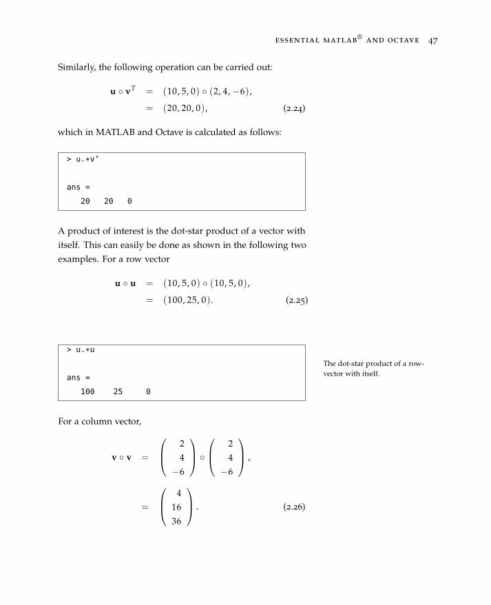
essential matlab®

and octave 47

Similarly, the following operation can be carried out:

u ◦ vT = (10, 5, 0) ◦ (2, 4,−6),

= (20, 20, 0), (2.24)

which in MATLAB and Octave is calculated as follows:

> u.*v’

ans =

20 20 0

A product of interest is the dot-star product of a vector with

itself. This can easily be done as shown in the following two

examples. For a row vector

u ◦ u = (10, 5, 0) ◦ (10, 5, 0),

= (100, 25, 0). (2.25)

The dot-star product of a row-vector with itself.

> u.*u

ans =

100 25 0

For a column vector,

v ◦ v =

2

4

−6

◦ 2

4

−6

,

=

4

16

36

. (2.26)

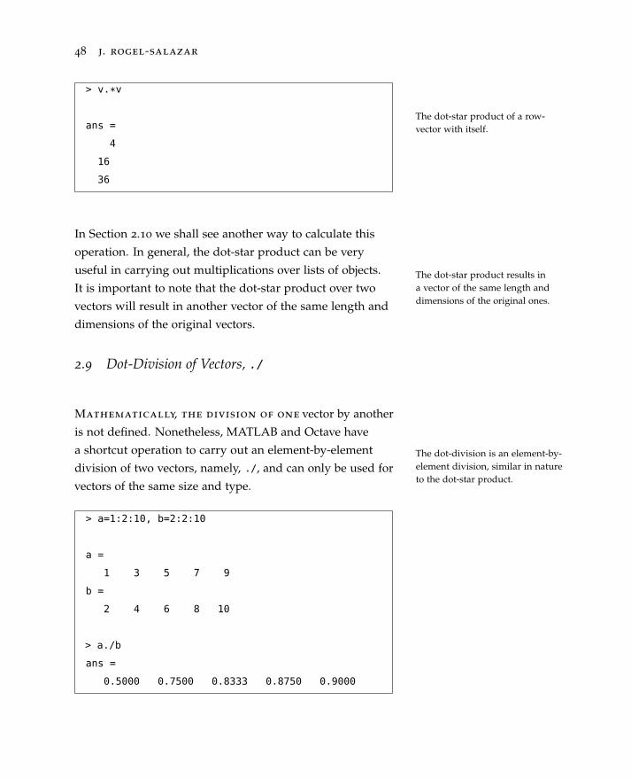
48 j. rogel-salazar

> v.*v

ans =

4

16

36

The dot-star product of a row-vector with itself.

In Section 2.10 we shall see another way to calculate this

operation. In general, the dot-star product can be very

useful in carrying out multiplications over lists of objects.

It is important to note that the dot-star product over two

vectors will result in another vector of the same length and

dimensions of the original vectors.

The dot-star product results ina vector of the same length anddimensions of the original ones.

2.9 Dot-Division of Vectors, ./

Mathematically, the division of one vector by another

is not defined. Nonetheless, MATLAB and Octave have

a shortcut operation to carry out an element-by-element

division of two vectors, namely, ./, and can only be used for

vectors of the same size and type.

The dot-division is an element-by-element division, similar in natureto the dot-star product.

> a=1:2:10, b=2:2:10

a =

1 3 5 7 9

b =

2 4 6 8 10

> a./b

ans =

0.5000 0.7500 0.8333 0.8750 0.9000

essential matlab®

and octave 49

Since division by zero is not defined, we must be careful

when implementing this operation:

Since division by zero is notdefined, we must be careful withthe dot-division operation.

> a./(b-6)

ans =

-0.2500 -1.5000 Inf 3.5000 2.2500

> c=-3:3

c =

-3 -2 -1 0 1 2 3

> c./c

ans =

1 1 1 NaN 1 1 1

In the first case we have ended up with an Inf in the result

as we have tried to divide by zero. In the second one the

result contains a NaN (Not a Number) as we have tried to

calculate 0/0.

As it is the case with the dot-star product, the implemen-

tation of the dot-division operation enables us to carry out

calculations over entire vectors in one single command. Let

us, for instance, tabulate the values of the function

y(x) =sin x

x. (2.27)

For simplicity we only show here a calculation with five

values:

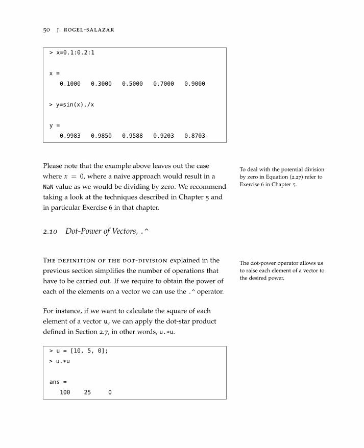
50 j. rogel-salazar

> x=0.1:0.2:1

x =

0.1000 0.3000 0.5000 0.7000 0.9000

> y=sin(x)./x

y =

0.9983 0.9850 0.9588 0.9203 0.8703

Please note that the example above leaves out the case

where x = 0, where a naive approach would result in a

NaN value as we would be dividing by zero. We recommend

taking a look at the techniques described in Chapter 5 and

in particular Exercise 6 in that chapter.

To deal with the potential divisionby zero in Equation (2.27) refer toExercise 6 in Chapter 5.

2.10 Dot-Power of Vectors, .^

The definition of the dot-division explained in the

previous section simplifies the number of operations that

have to be carried out. If we require to obtain the power of

each of the elements on a vector we can use the .^ operator.

The dot-power operator allows usto raise each element of a vector tothe desired power.

For instance, if we want to calculate the square of each

element of a vector u, we can apply the dot-star product

defined in Section 2.7, in other words, u.*u.

> u = [10, 5, 0];

> u.*u

ans =

100 25 0

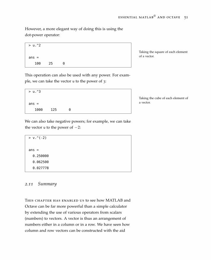
essential matlab®

and octave 51

However, a more elegant way of doing this is using the

dot-power operator:

Taking the square of each elementof a vector.

> u.^2

ans =

100 25 0

This operation can also be used with any power. For exam-

ple, we can take the vector u to the power of 3:

Taking the cube of each element ofa vector.

> u.^3

ans =

1000 125 0

We can also take negative powers; for example, we can take

the vector u to the power of −2:

> v.^(-2)

ans =

0.250000

0.062500

0.027778

2.11 Summary

This chapter has enabled us to see how MATLAB and

Octave can be far more powerful than a simple calculator

by extending the use of various operators from scalars

(numbers) to vectors. A vector is thus an arrangement of

numbers either in a column or in a row. We have seen how

column and row vectors can be constructed with the aid

52 j. rogel-salazar

of square brackets. Also, we have seen the power of the

colon notation (:) to define lists of numbers to be used in

the construction of vectors.

We have learnt how to extract elements of a vector by refer-

ring to the position of each element as in index. We have

also seen how arithmetic operations such as addition and

substraction can be directly applied to vectors. Furthermore,

we have covered further operations on vectors such as the

scalar product (*) and element-wise operations such as the

dot-star product (.*), dot-division (./) and dot-power (.^).

We have also seen how the orientation of the vectors can

make some of the operations mentioned above possible; in

order to deal correctly with some of those operations we

have introduced the transposition operator (’).

In the next chapter we will see how MATLAB and Octave

extend the capabilities of vector operations and manipula-

tions to more general arrays: matrices.

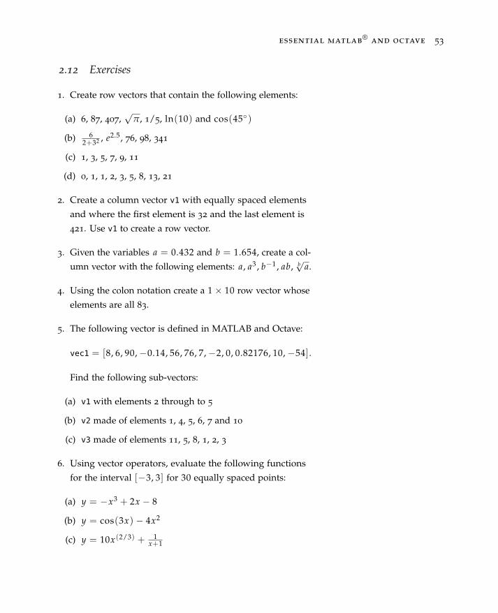
essential matlab®

and octave 53

2.12 Exercises

1. Create row vectors that contain the following elements:

(a) 6, 87, 407,√

π, 1/5, ln(10) and cos(45◦)

(b) 62+32 , e2.5, 76, 98, 341

(c) 1, 3, 5, 7, 9, 11

(d) 0, 1, 1, 2, 3, 5, 8, 13, 21

2. Create a column vector v1 with equally spaced elements

and where the first element is 32 and the last element is

421. Use v1 to create a row vector.

3. Given the variables a = 0.432 and b = 1.654, create a col-

umn vector with the following elements: a, a3 , b−1 , ab, b√

a.

4. Using the colon notation create a 1 × 10 row vector whose

elements are all 83.

5. The following vector is defined in MATLAB and Octave:

vec1 = [8, 6, 90,−0.14, 56, 76, 7,−2, 0, 0.82176, 10,−54].

Find the following sub-vectors:

(a) v1 with elements 2 through to 5

(b) v2 made of elements 1, 4, 5, 6, 7 and 10

(c) v3 made of elements 11, 5, 8, 1, 2, 3

6. Using vector operators, evaluate the following functions

for the interval [−3, 3] for 30 equally spaced points:

(a) y = −x3 + 2x − 8

(b) y = cos(3x) − 4x2

(c) y = 10x(2/3) + 1x+1

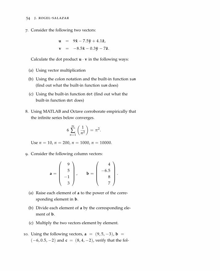
54 j. rogel-salazar

7. Consider the following two vectors:

u = 9x − 7.5y + 4.1z,

v = −8.5x − 0.3y − 7z.

Calculate the dot product u · v in the following ways:

(a) Using vector multiplication

(b) Using the colon notation and the built-in function sum

(find out what the built-in function sum does)

(c) Using the built-in function dot (find out what the

built-in function dot does)

8. Using MATLAB and Octave corroborate empirically that

the infinite series below converges.

6∞

∑n=1

(1

n2

)= π2 .

Use n = 10, n = 200, n = 1000, n = 10000.

9. Consider the following column vectors:

a =

9

5

−1

3

, b =

4

−6.5

8

7

.

(a) Raise each element of a to the power of the corre-

sponding element in b.

(b) Divide each element of a by the corresponding ele-

ment of b.

(c) Multiply the two vectors element by element.

10. Using the following vectors, a = (9, 5,−3), b =

(−6, 0.5,−2) and c = (8, 4,−2), verify that the fol-

essential matlab®

and octave 55

lowing vector identity holds:

a × (b × c) = b(a · c) − c(a · b)

Use the built-in function cross to calculate the cross-

product.

57

3

Matrices and Matrix Operators

In the previous chapter we saw how to define vectors in

MATLAB® and Octave as well as the way in which we can

manipulate and carry out operations with them. As it turns

out, row and column vectors are special cases of matrices.

An m × n matrix is a rectangular array of numbers having mrows and n columns:

A matrix can be thought of asa collection of row (or column)vectors.

A =

a1,1 a1,2 · · · a1,n

a2,1 a2,2 · · · a2,n...

.... . .

...

am,1 am,2 · · · am,n

. (3.1)

We can refer to m and n as the size of the matrix.

Let us consider the following 3 × 2 matrix:

A =

12 30

42 15

−3 −7

. (3.2)

We can enter this matrix into MATLAB and Octave one row

at a time and each row separated by a new line:

58 j. rogel-salazar

> A=[12 30

42 15

-3 -7]

A =

12 30

42 15

-3 -7

A matrix can be entered byseparating each row with a newline.

The same syntax that was used for vectors can be applied

here: instead of entering a new line to define a row, we can

simply separate the rows with semicolons.

Alternatively we can use semi-colons to separate each row.

> B=[9 8; 7 6; 5 4]

B =

9 8

7 6

5 4

> C=[1:3;4:6;7:9]

C =

1 2 3

4 5 6

7 8 9

In this way, the matrices defined above, namely, A and B, are A row-vector can be thought of asa 1× n array and a column vectoran m× 1 one.

3× 2 matrices whereas C is 3× 3. With this notation, we can

think of a row-vector as a 1× n array and a column vector is

an m× 1 matrix.

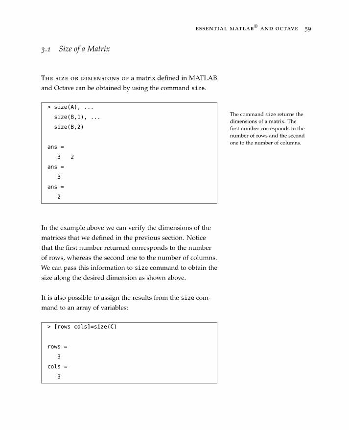
essential matlab®

and octave 59

3.1 Size of a Matrix

The size or dimensions of a matrix defined in MATLAB

and Octave can be obtained by using the command size.

The command size returns thedimensions of a matrix. Thefirst number corresponds to thenumber of rows and the secondone to the number of columns.

> size(A), ...

size(B,1), ...

size(B,2)

ans =

3 2

ans =

3

ans =

2

In the example above we can verify the dimensions of the

matrices that we defined in the previous section. Notice

that the first number returned corresponds to the number

of rows, whereas the second one to the number of columns.

We can pass this information to size command to obtain the

size along the desired dimension as shown above.

It is also possible to assign the results from the size com-

mand to an array of variables:

> [rows cols]=size(C)

rows =

3

cols =

3

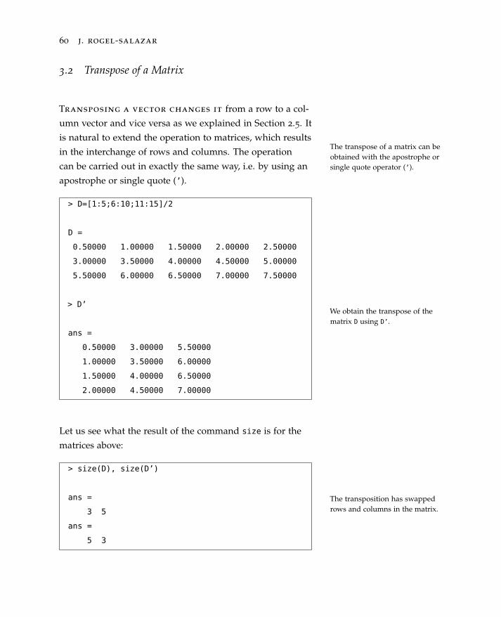
60 j. rogel-salazar

3.2 Transpose of a Matrix

Transposing a vector changes it from a row to a col-

umn vector and vice versa as we explained in Section 2.5. It

is natural to extend the operation to matrices, which results

in the interchange of rows and columns. The operation

can be carried out in exactly the same way, i.e. by using an

apostrophe or single quote (’).

The transpose of a matrix can beobtained with the apostrophe orsingle quote operator (’).

> D=[1:5;6:10;11:15]/2

D =

0.50000 1.00000 1.50000 2.00000 2.50000

3.00000 3.50000 4.00000 4.50000 5.00000

5.50000 6.00000 6.50000 7.00000 7.50000

> D’

ans =

0.50000 3.00000 5.50000

1.00000 3.50000 6.00000

1.50000 4.00000 6.50000

2.00000 4.50000 7.00000

We obtain the transpose of thematrix D using D’.

Let us see what the result of the command size is for the

matrices above:

The transposition has swappedrows and columns in the matrix.

> size(D), size(D’)

ans =

3 5

ans =

5 3

essential matlab®

and octave 61

An important aspect to consider when using the apostrophe

or single quote notation to calculate the transpose of an

array is the fact that when applied to a matrix with com- The complex conjugate transposeof a matrix can be obtained withthe apostrophe notation.

plex elements, the complex conjugate transpose is actually

calculated. For example, consider the matrix

E =

1 + i 2 + 3i 4 − 5i2 − 5i 6 − 6i 7 + i3 + 8i 9 − 10i 5 + 4i

(3.3)

whose complex conjugate transpose is given by

E∗ =

1 − i 2 + 5i 3 − 8i2 − 3i 6 + 6i 9 + 10i4 + 5i 7 − i 5 − 4i

. (3.4)

We can obtain the latter in MATLAB and Octave as follows:

> E=[1+1i 2+3*1i 4-5*1i; ...

2-5*1i 6-6*1i 7+1i; ...

3+8*1i 9-10*1i 5+4*1i]

E =

1 + 1i 2 + 3i 4 - 5i

2 - 5i 6 - 6i 7 + 1i

3 + 8i 9 - 10i 5 + 4i

> E_star = E’

E_star =

1 - 1i 2 + 5i 3 - 8i

2 - 3i 6 + 6i 9 + 10i

4 + 5i 7 - 1i 5 - 4i

We can obtain the direct transpose with the transpose

command as follows:

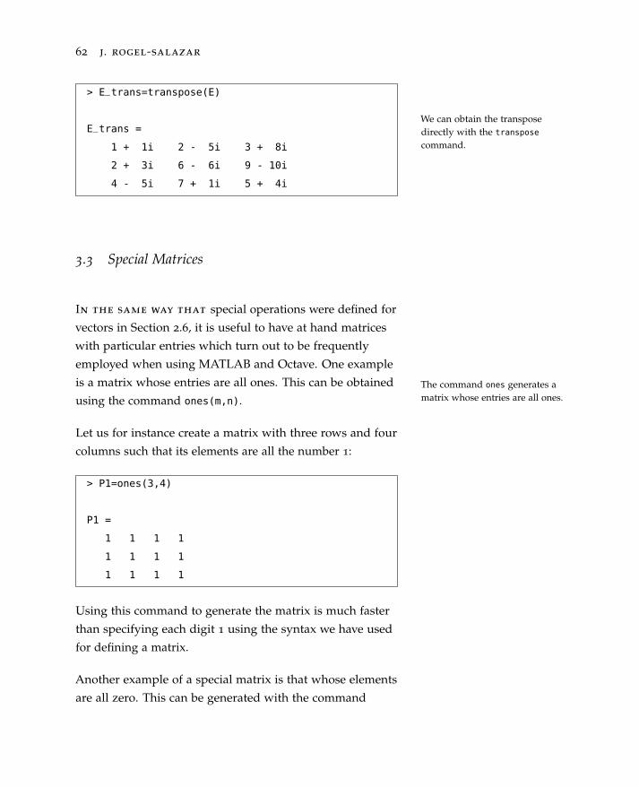
62 j. rogel-salazar

> E_trans=transpose(E)

E_trans =

1 + 1i 2 - 5i 3 + 8i

2 + 3i 6 - 6i 9 - 10i

4 - 5i 7 + 1i 5 + 4i

We can obtain the transposedirectly with the transpose

command.

3.3 Special Matrices

In the same way that special operations were defined for

vectors in Section 2.6, it is useful to have at hand matrices

with particular entries which turn out to be frequently

employed when using MATLAB and Octave. One example

is a matrix whose entries are all ones. This can be obtained

using the command ones(m,n).The command ones generates amatrix whose entries are all ones.

Let us for instance create a matrix with three rows and four

columns such that its elements are all the number 1:

> P1=ones(3,4)

P1 =

1 1 1 1

1 1 1 1

1 1 1 1

Using this command to generate the matrix is much faster

than specifying each digit 1 using the syntax we have used

for defining a matrix.

Another example of a special matrix is that whose elements

are all zero. This can be generated with the command

essential matlab®

and octave 63

zeros(m,n). We can for example create a 4 × 3 matrix whose

entries are all 0:The command zeros generates amatrix whose entries are all zero.

> Z1=zeros(4,3)

Z1 =

0 0 0

0 0 0

0 0 0

0 0 0

We can use the commands above together with the size

of a given matrix to generate a new matrix with the same

dimensions. Let us have a look at an example by creating a

couple of matrices with the same dimensions as the matrix D

defined in Section 3.2 whose dimensions were 3 × 5. In order

to do this we can combine size, that returns the dimensions

of the matrix, with the special matrices defined above:

> ones(size(D)), zeros(size(D))

ans =

1 1 1 1 1

1 1 1 1 1

1 1 1 1 1

ans =

0 0 0 0 0

0 0 0 0 0

0 0 0 0 0

We have combined the commandsize and the special matrices ones

and zeros to create two matriceswith the same dimensions ofmatrix as D defined above.

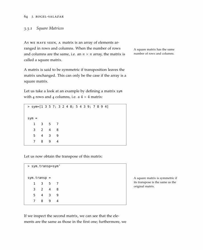
64 j. rogel-salazar

3.3.1 Square Matrices

As we have seen, a matrix is an array of elements ar-

ranged in rows and columns. When the number of rows

and columns are the same, i.e. an n × n array, the matrix is

called a square matrix.

A square matrix has the samenumber of rows and columns.

A matrix is said to be symmetric if transposition leaves the

matrix unchanged. This can only be the case if the array is a

square matrix.

Let us take a look at an example by defining a matrix sym

with 4 rows and 4 columns, i.e. a 4 × 4 matrix:

> sym=[1 3 5 7; 3 2 4 8; 5 4 3 9; 7 8 9 4]

sym =

1 3 5 7

3 2 4 8

5 4 3 9

7 8 9 4

Let us now obtain the transpose of this matrix:

A square matrix is symmetric ifits transpose is the same as theoriginal matrix.

> sym_transp=sym’

sym_transp =

1 3 5 7

3 2 4 8

5 4 3 9

7 8 9 4

If we inspect the second matrix, we can see that the ele-

ments are the same as those in the first one; furthermore, we

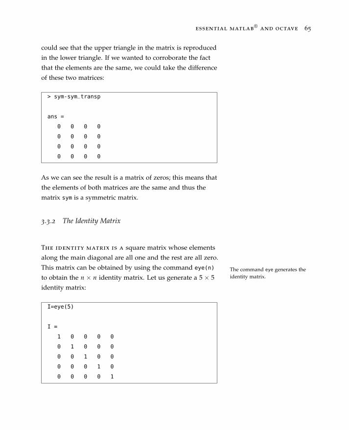
essential matlab®

and octave 65

could see that the upper triangle in the matrix is reproduced

in the lower triangle. If we wanted to corroborate the fact

that the elements are the same, we could take the difference

of these two matrices:

> sym-sym_transp

ans =

0 0 0 0

0 0 0 0

0 0 0 0

0 0 0 0

As we can see the result is a matrix of zeros; this means that

the elements of both matrices are the same and thus the

matrix sym is a symmetric matrix.

3.3.2 The Identity Matrix

The identity matrix is a square matrix whose elements

along the main diagonal are all one and the rest are all zero.

This matrix can be obtained by using the command eye(n)

to obtain the n × n identity matrix. Let us generate a 5 × 5

identity matrix:

The command eye generates theidentity matrix.

I=eye(5)

I =

1 0 0 0 0

0 1 0 0 0

0 0 1 0 0

0 0 0 1 0

0 0 0 0 1

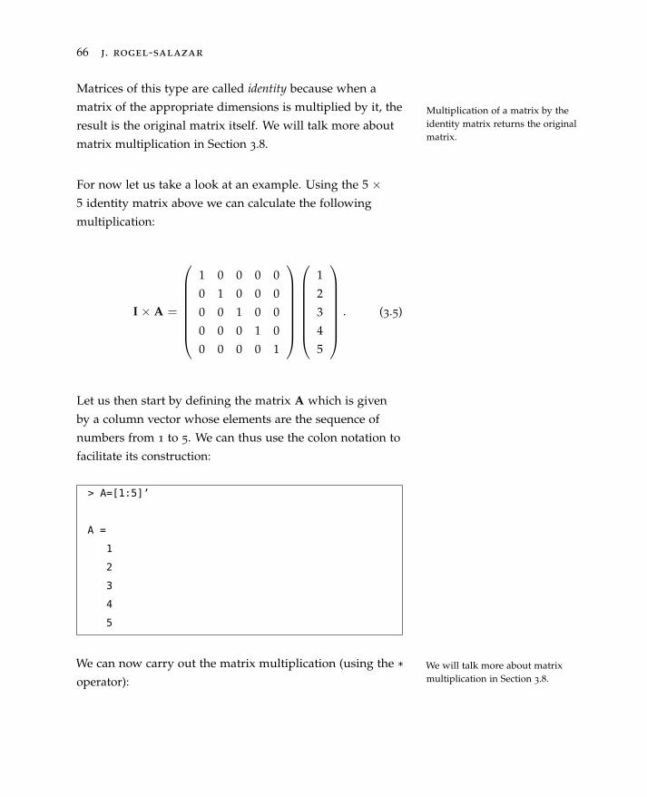
66 j. rogel-salazar

Matrices of this type are called identity because when a

matrix of the appropriate dimensions is multiplied by it, the

result is the original matrix itself. We will talk more about

matrix multiplication in Section 3.8.

Multiplication of a matrix by theidentity matrix returns the originalmatrix.

For now let us take a look at an example. Using the 5 ×5 identity matrix above we can calculate the following

multiplication:

I × A =

1 0 0 0 0

0 1 0 0 0

0 0 1 0 0

0 0 0 1 0

0 0 0 0 1

1

2

3

4

5

. (3.5)

Let us then start by defining the matrix A which is given

by a column vector whose elements are the sequence of

numbers from 1 to 5. We can thus use the colon notation to

facilitate its construction:

> A=[1:5]’

A =

1

2

3

4

5

We can now carry out the matrix multiplication (using the *

operator):We will talk more about matrixmultiplication in Section 3.8.

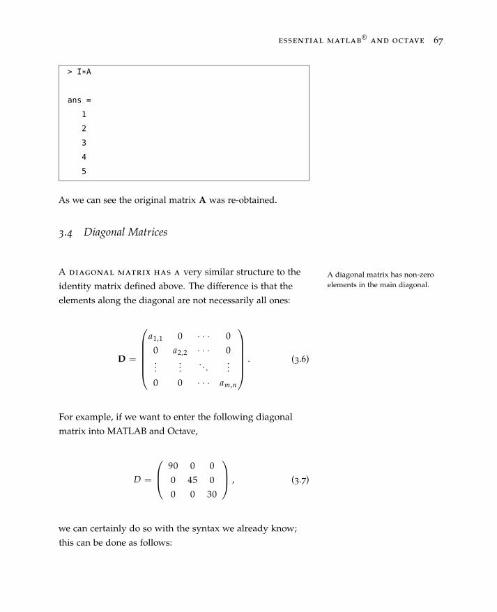
essential matlab®

and octave 67

> I*A

ans =

1

2

3

4

5

As we can see the original matrix A was re-obtained.

3.4 Diagonal Matrices

A diagonal matrix has a very similar structure to the

identity matrix defined above. The difference is that the

elements along the diagonal are not necessarily all ones:

A diagonal matrix has non-zeroelements in the main diagonal.

D =

a1,1 0 · · · 0

0 a2,2 · · · 0...

.... . .

...

0 0 · · · am,n

. (3.6)

For example, if we want to enter the following diagonal

matrix into MATLAB and Octave,

D =

90 0 0

0 45 0

0 0 30

, (3.7)

we can certainly do so with the syntax we already know;

this can be done as follows:

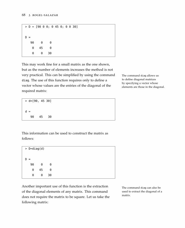
68 j. rogel-salazar

> D = [90 0 0; 0 45 0; 0 0 30]

D =

90 0 0

0 45 0

0 0 30

This may work fine for a small matrix as the one shown,

but as the number of elements increases the method is not

very practical. This can be simplified by using the command

diag. The use of this function requires only to define aThe command diag allows usto define diagonal matricesby specifying a vector whoseelements are those in the diagonal.vector whose values are the entries of the diagonal of the

required matrix:

> d=[90, 45 30]

d =

90 45 30

This information can be used to construct the matrix as

follows:

> D=diag(d)

D =

90 0 0

0 45 0

0 0 30

Another important use of this function is the extraction

of the diagonal elements of any matrix. This command

does not require the matrix to be square. Let us take the

following matrix:

The command diag can also beused to extract the diagonal of amatrix.

essential matlab®

and octave 69

> sym=[1 3 5 7; 3 2 4 8; 5 4 3 9; 7 8 9 4]

sym =

1 3 5 7

3 2 4 8

5 4 3 9

7 8 9 4

We can easily see that the diagonal elements are 1, 2, 3, 4.

These elements can be extracted with the help of the diag

command as follows:

> diag(sym)

ans =

1

2

3

4

Another important use of the diag command is the manipu-

lation of off-diagonal elements. Let us consider constructing

the following matrix:

D1 =

0 1 0 0 0

0 0 2 0 0

0 0 0 3 0

0 0 0 0 4

0 0 0 0 0

, (3.8)

which can easily be created with the use of the diag(v,k) diag(v,k) enables us to con-struct matrices with off-diagonalelements.

command, whose first argument v is a vector containing

the elements in the diagonal, and the second argument k

corresponds to the kth diagonal of the matrix, with k = 0

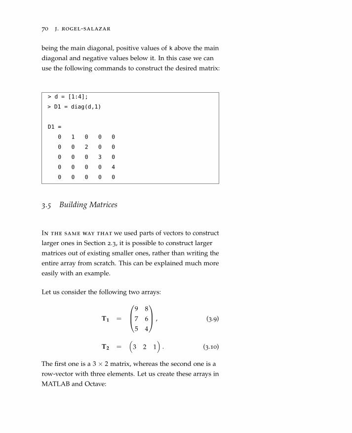
70 j. rogel-salazar

being the main diagonal, positive values of k above the main

diagonal and negative values below it. In this case we can

use the following commands to construct the desired matrix:

> d = [1:4];

> D1 = diag(d,1)

D1 =

0 1 0 0 0

0 0 2 0 0

0 0 0 3 0

0 0 0 0 4

0 0 0 0 0

3.5 Building Matrices

In the same way that we used parts of vectors to construct

larger ones in Section 2.3, it is possible to construct larger

matrices out of existing smaller ones, rather than writing the

entire array from scratch. This can be explained much more

easily with an example.

Let us consider the following two arrays:

T1 =

9 8

7 6

5 4

, (3.9)

T2 =(

3 2 1)

. (3.10)

The first one is a 3 × 2 matrix, whereas the second one is a

row-vector with three elements. Let us create these arrays in

MATLAB and Octave:

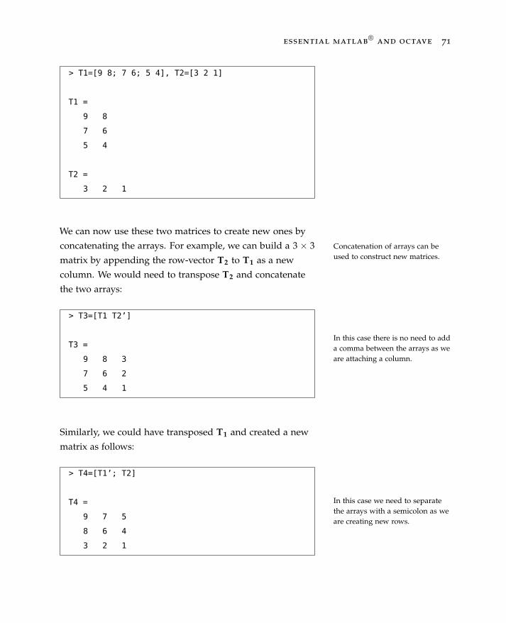
essential matlab®

and octave 71

> T1=[9 8; 7 6; 5 4], T2=[3 2 1]

T1 =

9 8

7 6

5 4

T2 =

3 2 1

We can now use these two matrices to create new ones by

concatenating the arrays. For example, we can build a 3 × 3 Concatenation of arrays can beused to construct new matrices.matrix by appending the row-vector T2 to T1 as a new

column. We would need to transpose T2 and concatenate

the two arrays:

> T3=[T1 T2’]

T3 =

9 8 3

7 6 2

5 4 1

In this case there is no need to adda comma between the arrays as weare attaching a column.

Similarly, we could have transposed T1 and created a new

matrix as follows:

In this case we need to separatethe arrays with a semicolon as weare creating new rows.

> T4=[T1’; T2]

T4 =

9 7 5

8 6 4

3 2 1

72 j. rogel-salazar

This method works for larger arrangements. Consider for

example the following matrix:

p =

1 2 3

4 6 8

12 13 144

. (3.11)

From this matrix we can think of constructing the following

one:

pnew =

1 0 0 1 2 3

0 2 0 4 6 8

0 0 3 12 13 14

0 0 0 1 4 12

0 0 0 2 6 13

0 0 0 3 8 14

. (3.12)

This can be achieved by manipulating the elements of the pmatrix with the commands we have seen so far as follows:

The concatenation of matrices canbe used to construct larger arrays,too.

> p=[1:3; 4:2:9; 12 13 14]

p =

1 2 3

4 6 8

12 13 14

> p_new=[diag(1:3) p; zeros(3) p’]

p_new =

1 0 0 1 2 3

0 2 0 4 6 8

0 0 3 12 13 14

0 0 0 1 4 12

0 0 0 2 6 13

0 0 0 3 8 14

essential matlab®

and octave 73

It is sometimes useful to visualise the non-zero entries of

a matrix, particularly those with a large number of elements.

We can obtain a visualisation in a Cartesian plane by ap-

plying the command spy. In the case above, if we issue the The built-in function spy lets usvisualise structure of a matrix.command spy(p_new) MATLAB and Octave will generate a

plot similar to that shown in Figure 3.1.

0 1 2 3 4 5 6 7

0

1

2

3

4

5

6

7

nz = 21

Figure 3.1: Non-zero elementsof the matrix p_new definedin the text. The command spy

can be used to obtain a visualrepresentation of the non-zeroelements of a matrix.

3.6 Tabulating Functions

We are now familiar with the way MATLAB and Octave

deal with arrays of numbers in columns and rows. We can

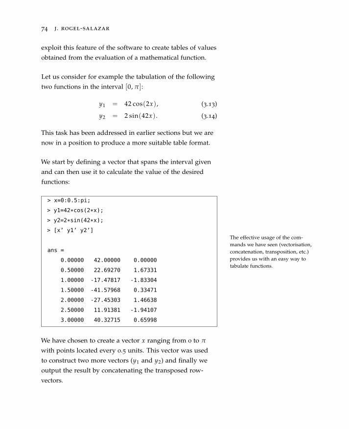
74 j. rogel-salazar

exploit this feature of the software to create tables of values

obtained from the evaluation of a mathematical function.

Let us consider for example the tabulation of the following

two functions in the interval [0, π ]:

y1 = 42 cos(2x), (3.13)

y2 = 2 sin(42x). (3.14)

This task has been addressed in earlier sections but we are

now in a position to produce a more suitable table format.

We start by defining a vector that spans the interval given

and can then use it to calculate the value of the desired

functions:

The effective usage of the com-mands we have seen (vectorisation,concatenation, transposition, etc.)provides us with an easy way totabulate functions.

> x=0:0.5:pi;

> y1=42*cos(2*x);

> y2=2*sin(42*x);

> [x’ y1’ y2’]

ans =

0.00000 42.00000 0.00000

0.50000 22.69270 1.67331

1.00000 -17.47817 -1.83304

1.50000 -41.57968 0.33471

2.00000 -27.45303 1.46638

2.50000 11.91381 -1.94107

3.00000 40.32715 0.65998

We have chosen to create a vector x ranging from 0 to π

with points located every 0.5 units. This vector was used

to construct two more vectors (y1 and y2) and finally we

output the result by concatenating the transposed row-

vectors.

essential matlab®

and octave 75

We can increase the number of values by changing the step

in the first command. A similar result could have been

obtained with the command [x; y; u;]’ or by transposing

the vector x at the beginning, i.e. x=(0:0.5:pi)’.

Remember that there are multipleways to obtain the same result.

3.7 Extracting Parts of Matrices

The way in which MATLAB and Octave treat vectors can

readily be applied to matrices, for example in the extraction

of elements from matrices. The discussion here follows the

one presented in Section 2.3.

In order to extract parts of matrices we have to take into

account that each and every element of a matrix is indexed

according to the row and column where it is positioned.

In this way, A(r,c) refers to the element in the r th row and

cth column of the matrix A. In MATLAB and Octave this is

denoted by A(r,c).

Let us consider an example: Given the matrix

Element extraction relies on theindexation of the elements interms of rows and columns.

A =

16 2 3 13

5 11 10 8

9 7 6 12

4 14 15 1

, (3.15)

we can see that the element in the first row and first column

is A(1,1) = 16, the element in row 4, column 3 is A(4,3) =

15 and the element in row 3, column 1 is A(3,1) = 9.

This can also be achieved in MATLAB and Octave. First, we

note that the matrix A above is in fact a 4 × 4 magic matrix,

and as such we can easily create it with the use of the magic

command:

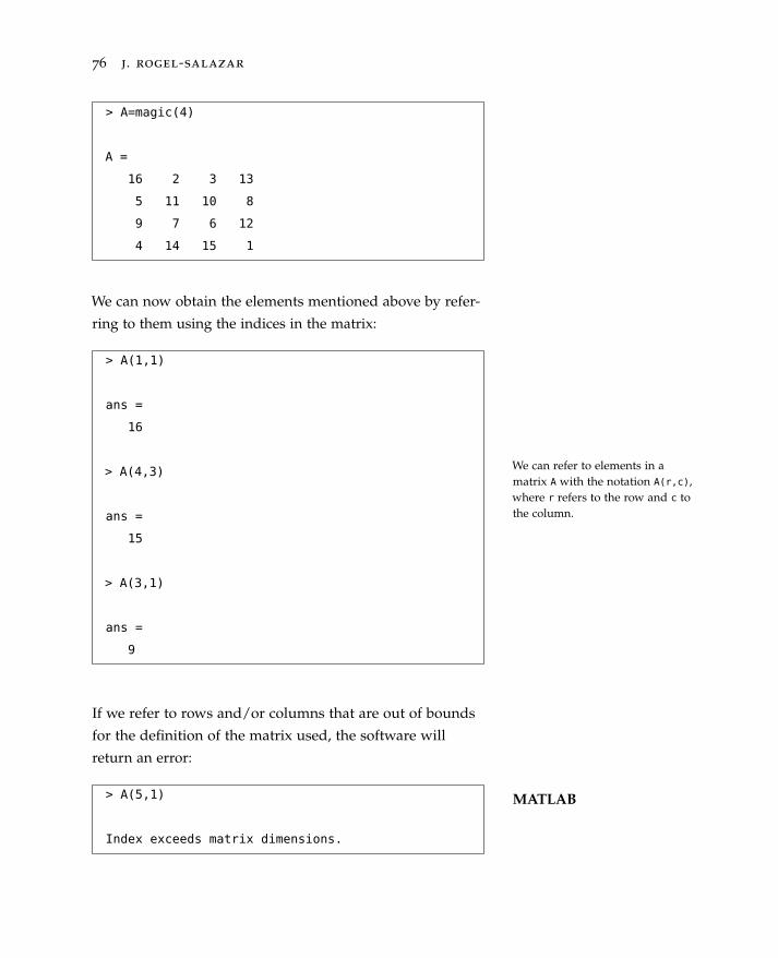
76 j. rogel-salazar

> A=magic(4)

A =

16 2 3 13

5 11 10 8

9 7 6 12

4 14 15 1

We can now obtain the elements mentioned above by refer-

ring to them using the indices in the matrix:

> A(1,1)

ans =

16

> A(4,3)

ans =

15

> A(3,1)

ans =

9

We can refer to elements in amatrix A with the notation A(r,c),where r refers to the row and c tothe column.

If we refer to rows and/or columns that are out of bounds

for the definition of the matrix used, the software will

return an error:

MATLAB> A(5,1)

Index exceeds matrix dimensions.

essential matlab®

and octave 77

Octave> A(5,1)

error: A(I,J): row index out of bounds;

value 5 out of bound 4

We can also carry out operations with individual elements

of the matrix. For example, let us imagine that we require

the element A(1,1) to be equal to the element A(4,4) + 9; we

can do this by operating on the element alone as follows:

> A(1,1) = A(4,4) + 9;

Note that the operation above only affected that particular

element in the matrix. We can corroborate this by displaying

the full matrix A:

> A

A =

10 2 3 13

5 11 10 8

9 7 6 12

4 14 15 1

Let us see another example. We want the element A(4,4) to

be three times A(2,2) and subtract the value of A(1,1) .

The operation on individualmatrix elements only affects thoseelements alone.

> A(4,4)=3*A(2,2)-A(1,1)

A =

10 2 3 13

5 11 10 8

9 7 6 12

4 14 15 23

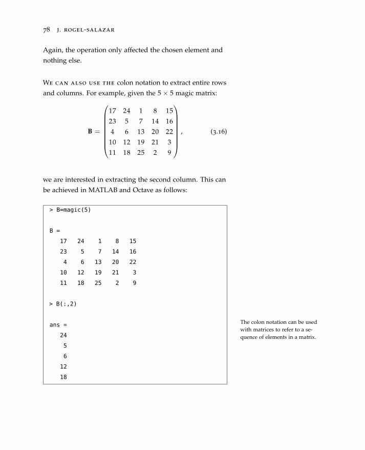
78 j. rogel-salazar

Again, the operation only affected the chosen element and

nothing else.

We can also use the colon notation to extract entire rows

and columns. For example, given the 5 × 5 magic matrix:

B =

17 24 1 8 15

23 5 7 14 16

4 6 13 20 22

10 12 19 21 3

11 18 25 2 9

, (3.16)

we are interested in extracting the second column. This can

be achieved in MATLAB and Octave as follows:

> B=magic(5)

B =

17 24 1 8 15

23 5 7 14 16

4 6 13 20 22

10 12 19 21 3

11 18 25 2 9

> B(:,2)

ans =

24

5

6

12

18

The colon notation can be usedwith matrices to refer to a se-quence of elements in a matrix.

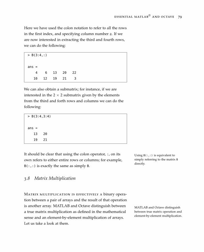
essential matlab®

and octave 79

Here we have used the colon notation to refer to all the rows

in the first index, and specifying column number 2. If we

are now interested in extracting the third and fourth rows,

we can do the following:

> B(3:4,:)

ans =

4 6 13 20 22

10 12 19 21 3

We can also obtain a submatrix; for instance, if we are

interested in the 2 × 2 submatrix given by the elements

from the third and forth rows and columns we can do the

following:

> B(3:4,3:4)

ans =

13 20

19 21

It should be clear that using the colon operator, :, on its

own refers to either entire rows or columns; for example,

B(:,:) is exactly the same as simply B.

Using B(:,:) is equivalent tosimply referring to the matrix B

directly.

3.8 Matrix Multiplication

Matrix multiplication is effectively a binary opera-

tion between a pair of arrays and the result of that operation

is another array. MATLAB and Octave distinguish between

a true matrix multiplication as defined in the mathematical

sense and an element-by-element multiplication of arrays.

Let us take a look at them.

MATLAB and Octave distinguishbetween true matrix operation andelement-by-element multiplication.

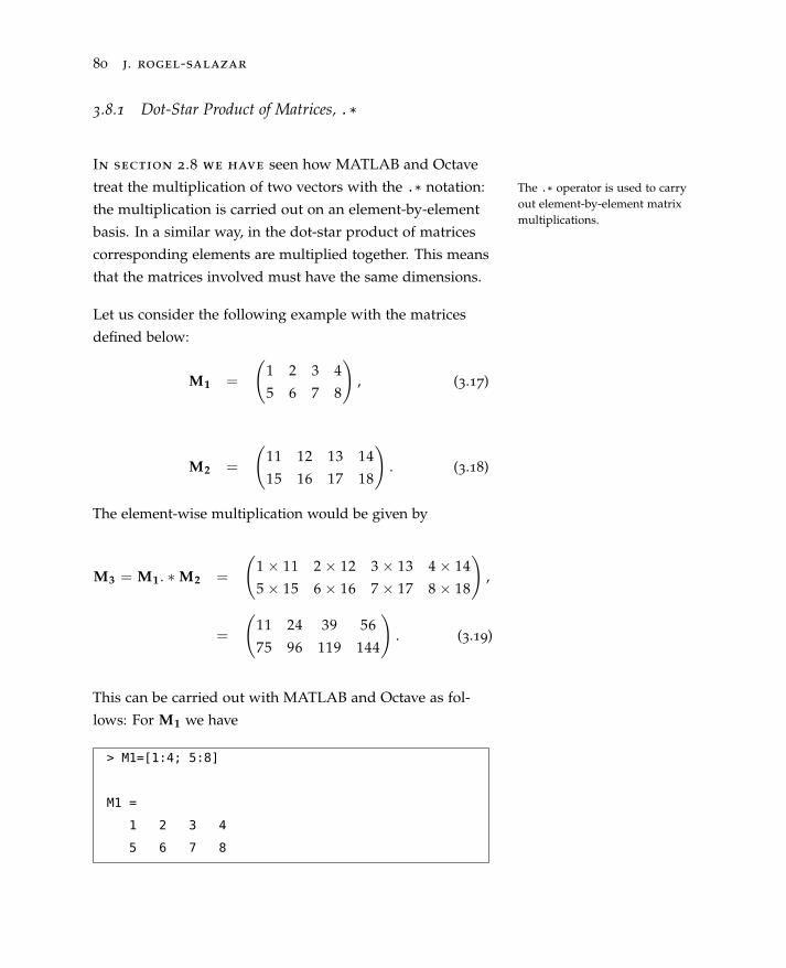
80 j. rogel-salazar

3.8.1 Dot-Star Product of Matrices, .*

In section 2.8 we have seen how MATLAB and Octave

treat the multiplication of two vectors with the .* notation: The .* operator is used to carryout element-by-element matrixmultiplications.

the multiplication is carried out on an element-by-element

basis. In a similar way, in the dot-star product of matrices

corresponding elements are multiplied together. This means

that the matrices involved must have the same dimensions.

Let us consider the following example with the matrices

defined below:

M1 =

(1 2 3 4

5 6 7 8

), (3.17)

M2 =

(11 12 13 14

15 16 17 18

). (3.18)

The element-wise multiplication would be given by

M3 = M1 . ∗M2 =

(1 × 11 2 × 12 3 × 13 4 × 14

5 × 15 6 × 16 7 × 17 8 × 18

),

=

(11 24 39 56

75 96 119 144

). (3.19)

This can be carried out with MATLAB and Octave as fol-

lows: For M1 we have

> M1=[1:4; 5:8]

M1 =

1 2 3 4

5 6 7 8

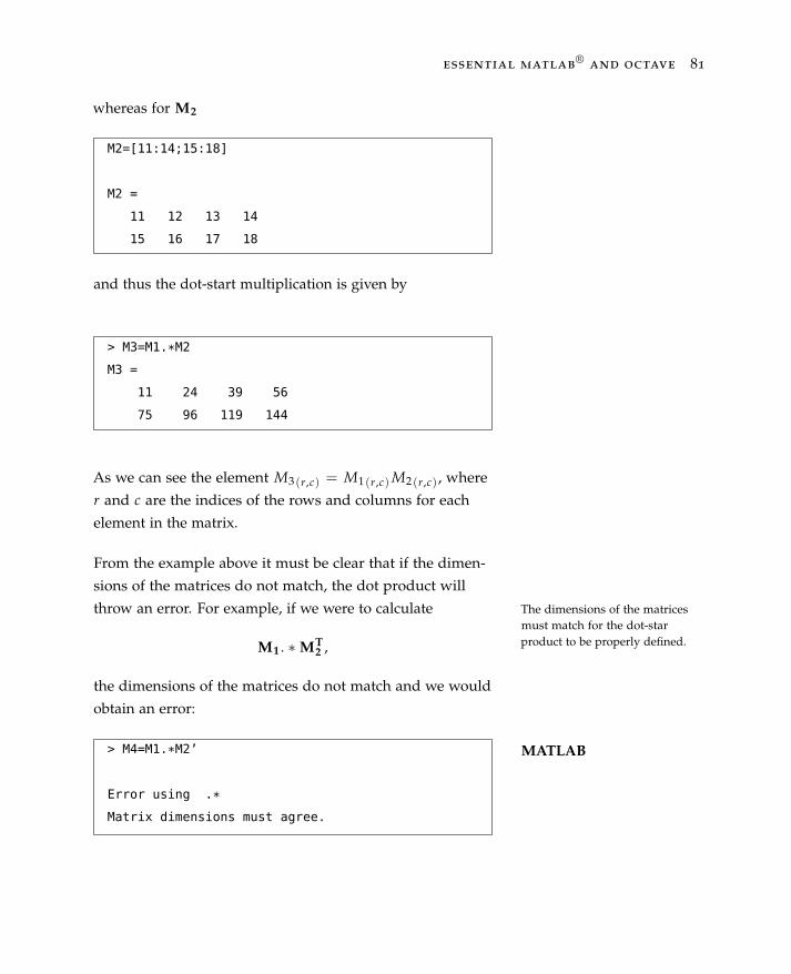
essential matlab®

and octave 81

whereas for M2

M2=[11:14;15:18]

M2 =

11 12 13 14

15 16 17 18

and thus the dot-start multiplication is given by

> M3=M1.*M2

M3 =

11 24 39 56

75 96 119 144

As we can see the element M3 (r,c) = M1 (r,c)M2 (r,c) , where

r and c are the indices of the rows and columns for each

element in the matrix.

From the example above it must be clear that if the dimen-

sions of the matrices do not match, the dot product will

throw an error. For example, if we were to calculate The dimensions of the matricesmust match for the dot-starproduct to be properly defined.M1 . ∗MT

2 ,

the dimensions of the matrices do not match and we would

obtain an error:

MATLAB> M4=M1.*M2’

Error using .*

Matrix dimensions must agree.

82 j. rogel-salazar

Octave> M4=M1.*M2’

error: product: nonconformant arguments

(op1 is 2x4, op2 is 4x2)

In the examples above we have transposed the matrix M2

which makes the product undefined.

3.8.2 Matrix-Vector Products

A vector is an array whose elements are arranged

either in a row or in a column. We can therefore define the

product of a matrix with a vector and it must be clear that

this product can only be defined if a column vector has the

same number of elements as the matrix has columns.

In other words, if the matrix A is an m × n matrix and x is

a column vector of length n, then the matrix-vector product

Ax can indeed be performed. In this manner, an m × n

Given appropriate dimensions, theproduct of a matrix and a vector iswell defined.

matrix times an n × 1 matrix results in an m × 1 matrix. For

example, given the following arrays:

A =

7 1 4

11 79 42

10 15 20

, (3.20)

x =

32

15

9

, (3.21)

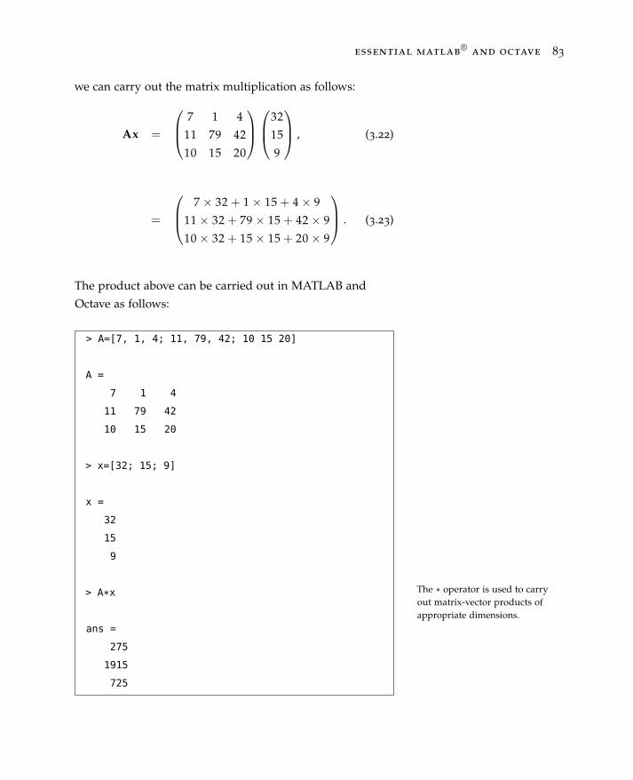
essential matlab®

and octave 83

we can carry out the matrix multiplication as follows:

Ax =

7 1 4

11 79 42

10 15 20

32

15

9

, (3.22)

=

7 × 32 + 1 × 15 + 4 × 9

11 × 32 + 79 × 15 + 42 × 9

10 × 32 + 15 × 15 + 20 × 9

. (3.23)

The product above can be carried out in MATLAB and

Octave as follows:

The * operator is used to carryout matrix-vector products ofappropriate dimensions.

> A=[7, 1, 4; 11, 79, 42; 10 15 20]

A =

7 1 4

11 79 42

10 15 20

> x=[32; 15; 9]

x =

32

15

9

> A*x

ans =

275

1915

725

84 j. rogel-salazar

Let us emphasise that the matrix-vector product is not

commutative and in some cases not only would the result

be different, but it may not even be defined, as we can see in

the following example:

MATLAB> x*A

Error using *

Inner matrix dimensions must agree.

Octave> x*A

error: operator *:

nonconformant arguments (op1 is 3x1, op2 is 3x3)

We obtained this error because the multiplication of the

vector x with the matrix A does not fulfil the condition

stated above about the dimensions of the arrays involved.

If the dimensions of the arrays donot match the software will throwan error.

3.8.3 Matrix-Matrix Products

We can think of a matrix as a group of column vectors

placed next to each other. In that way, the definition of a

matrix-matrix product is an extension of the matrix-vector

multiplication we have seen in the previous section. The

product of an m× n matrix A and an n× p matrix B, written

as AB, results in m × p matrix. The number of columns of The matrix-matrix product iscarried out in the same way as thematrix-vector one.

matrix A must match the number of rows of matrix B.

Let us look at an example: with the matrix A defined above

in Expression (3.20),

A =

7 1 4

11 79 42

10 15 20

,

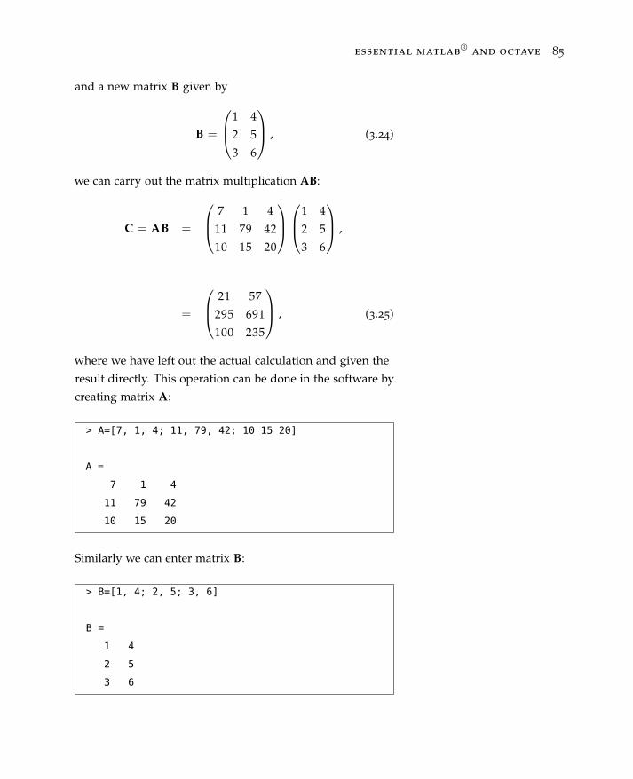
essential matlab®

and octave 85

and a new matrix B given by

B =

1 4

2 5

3 6

, (3.24)

we can carry out the matrix multiplication AB:

C = AB =

7 1 4

11 79 42

10 15 20

1 4

2 5

3 6

,

=

21 57

295 691

100 235

, (3.25)

where we have left out the actual calculation and given the

result directly. This operation can be done in the software by

creating matrix A:

> A=[7, 1, 4; 11, 79, 42; 10 15 20]

A =

7 1 4

11 79 42

10 15 20

Similarly we can enter matrix B:

> B=[1, 4; 2, 5; 3, 6]

B =

1 4

2 5

3 6

86 j. rogel-salazar

and thus the matrix-matrix multiplication can be performed

with the * operator:

> C=A*B

C =

21 57

295 691

100 235

The * operator is able to performmatrix-matrix multiplications withappropriate dimensions.

The matrix C above is the result of a 3 × 3 by a 3 × 2 matrix,

and thus it is a 3 × 2 array. If we try to obtain the multipli-

cation of BA we will obtain an error as the dimensions do

not match. However, if we transpose B the product can be

carried out:

Once again, care must be takenwith matching the dimensions ofthe matrices to be multiplied.

> D=B’*A

D =

59 204 148

143 489 346

3.9 Sparse Matrices

In a number of applications in physics, engineering,

finance, etc., it is quite common to deal with big matrices

with a large number of zero elements. These type of matri-

ces are called sparse matrices. The computational expense

when carrying out operations with these kind of matrices

can be quite high and that is why MATLAB and Octave

include a number of techniques to deal with them in a more

effective manner.

essential matlab®

and octave 87

Let us consider a 6 × 6 matrix S with only four non-zero

values: S(1,1) = 1, S(3,4) = 3, S(4,5) = 42 and S(6,1) = 7,

and therefore the 32 other elements are zero. Let us take a

look at this matrix:

S =

1 0 0 0 0

0 0 0 0 0

0 0 0 3 0

0 0 0 0 42

0 0 0 0 0

7 0 0 0 0

. (3.26)

The matrix shown has a largenumber of elements equal to zero.This can be better handled as asparse matrix.

If we wanted to enter this matrix in the software we can

indeed list every single element (including the 32 zeros), but

this is not a very effective way of entering such a matrix and

larger examples can get too cumbersome. Alternatively, we

can define a matrix with the command zeros and modify

the non-zero entries individually. With larger arrays we

also have the added problem of available memory and in

these cases it is better to define a sparse matrix, i.e. a matrix

where only the non-zero values are specified.

One easy way to define the matrix used in this example is to

define three vectors:

1. A vector that contains the row indices of the non-zero

elements

2. A vector that contains the column indices of the non-zero

elements

3. A vector that holds the values of each of the non-zero

elements of the matrix

With this information, we can now use the command sparse

to build the desired matrix. We can define the row indices:

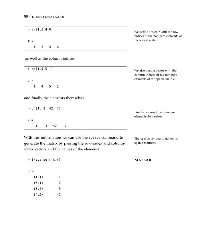
88 j. rogel-salazar

> r=[1,3,4,6]

r =

1 3 4 6

as well as the column indices:

We define a vector with the rowindices of the non-zero elements ofthe sparse matrix.

We also need a vector with thecolumn indices of the non-zeroelements of the sparse matrix.

> c=[1,4,5,1]

c =

1 4 5 1

and finally the elements themselves:

Finally, we need the non-zeroelements themselves.

> v=[1, 3, 42, 7]

v =

1 3 42 7

With this information we can use the sparse command to

generate the matrix by passing the row-index and column-

index vectors and the values of the elements:

The sparse command generatessparse matrices.

MATLAB> S=sparse(r,c,v)

S =

(1,1) 1

(6,1) 7

(3,4) 3

(4,5) 42

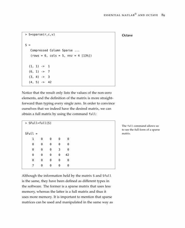
essential matlab®

and octave 89

Octave> S=sparse(r,c,v)

S =

Compressed Column Sparse ...

(rows = 6, cols = 5, nnz = 4 [13%])

(1, 1) -> 1

(6, 1) -> 7

(3, 4) -> 3

(4, 5) -> 42

Notice that the result only lists the values of the non-zero

elements, and the definition of the matrix is more straight-

forward than typing every single zero. In order to convince

ourselves that we indeed have the desired matrix, we can

obtain a full matrix by using the command full:

The full command allows usto see the full form of a sparsematrix.

> SFull=full(S)

SFull =

1 0 0 0 0

0 0 0 0 0

0 0 0 3 0

0 0 0 0 42

0 0 0 0 0

7 0 0 0 0

Although the information held by the matrix S and Sfull

is the same, they have been defined as different types in

the software. The former is a sparse matrix that uses less

memory, whereas the latter is a full matrix and thus it

uses more memory. It is important to mention that sparse

matrices can be used and manipulated in the same way as

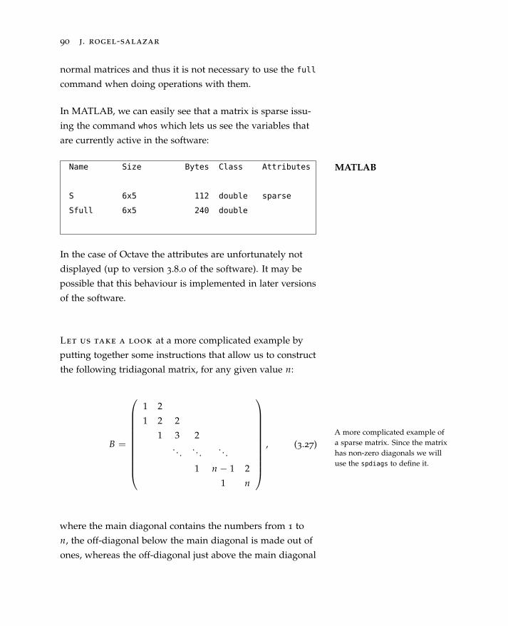
90 j. rogel-salazar

normal matrices and thus it is not necessary to use the full

command when doing operations with them.

In MATLAB, we can easily see that a matrix is sparse issu-

ing the command whos which lets us see the variables that

are currently active in the software:

MATLABName Size Bytes Class Attributes

S 6x5 112 double sparse

Sfull 6x5 240 double

In the case of Octave the attributes are unfortunately not

displayed (up to version 3.8.0 of the software). It may be

possible that this behaviour is implemented in later versions

of the software.

Let us take a look at a more complicated example by

putting together some instructions that allow us to construct

the following tridiagonal matrix, for any given value n:

B =

1 2

1 2 2

1 3 2. . . . . . . . .

1 n − 1 2

1 n

, (3.27)

A more complicated example ofa sparse matrix. Since the matrixhas non-zero diagonals we willuse the spdiags to define it.

where the main diagonal contains the numbers from 1 to

n, the off-diagonal below the main diagonal is made out of

ones, whereas the off-diagonal just above the main diagonal

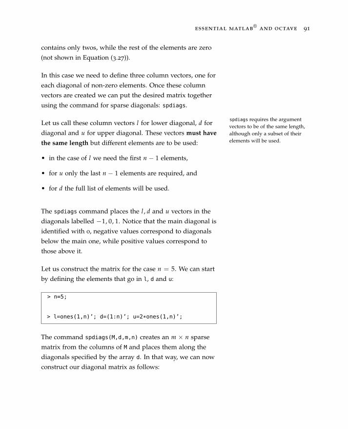
essential matlab®

and octave 91

contains only twos, while the rest of the elements are zero

(not shown in Equation (3.27)).

In this case we need to define three column vectors, one for

each diagonal of non-zero elements. Once these column

vectors are created we can put the desired matrix together

using the command for sparse diagonals: spdiags.

Let us call these column vectors l for lower diagonal, d for

diagonal and u for upper diagonal. These vectors must havethe same length but different elements are to be used:

spdiags requires the argumentvectors to be of the same length,although only a subset of theirelements will be used.

• in the case of l we need the first n − 1 elements,

• for u only the last n − 1 elements are required, and

• for d the full list of elements will be used.

The spdiags command places the l , d and u vectors in the

diagonals labelled −1, 0, 1. Notice that the main diagonal is

identified with 0, negative values correspond to diagonals

below the main one, while positive values correspond to

those above it.

Let us construct the matrix for the case n = 5. We can start

by defining the elements that go in l, d and u:

> n=5;

> l=ones(1,n)’; d=(1:n)’; u=2*ones(1,n)’;

The command spdiags(M,d,m,n) creates an m × n sparse

matrix from the columns of M and places them along the

diagonals specified by the array d. In that way, we can now

construct our diagonal matrix as follows:

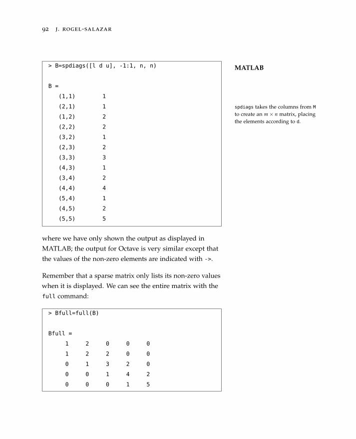
92 j. rogel-salazar

MATLAB> B=spdiags([l d u], -1:1, n, n)

B =

(1,1) 1

(2,1) 1

(1,2) 2

(2,2) 2

(3,2) 1

(2,3) 2

(3,3) 3

(4,3) 1

(3,4) 2

(4,4) 4

(5,4) 1

(4,5) 2

(5,5) 5

where we have only shown the output as displayed in

spdiags takes the columns from M

to create an m× n matrix, placingthe elements according to d.

MATLAB; the output for Octave is very similar except that

the values of the non-zero elements are indicated with ->.

Remember that a sparse matrix only lists its non-zero values

when it is displayed. We can see the entire matrix with the

full command:

> Bfull=full(B)

Bfull =

1 2 0 0 0

1 2 2 0 0

0 1 3 2 0

0 0 1 4 2

0 0 0 1 5

essential matlab®

and octave 93

3.10 Systems of Linear Equations

Now that we know how to enter matrices in MATLAB

and Octave it becomes natural to ask the software to solve

a linear system of equations given that such systems can be

written in terms of matrices.

A general system of linear equations can be expressed in

terms of a coefficient matrix A, a column vector b and a

column vector of unknowns x such that

The use of matrices in solvinglinear systems becomes quitenatural in MATLAB and Octave.

Ax = b (3.28)

or, expanding the matrix multiplication,

a1,1x1 + a1,2x2 + · · ·+ a1,nxn = b1, (3.29)

a2,1x1 + a2,2x2 + · · ·+ a2,nxn = b2,...

an,1x1 + an,2x2 + · · ·+ an,nxn = bn.

When A is non-singular and square (n× n), meaning that the

number of independent equations is equal to the number of

unknowns, the system has a unique solution given by

x = A−1b, (3.30)

where A−1 is the inverse of the matrix A. This means that

the solution vector x can be calculated by taking the inverse

of the coefficient matrix A and multiplying it from the right

with vector b. Although this method seems to be quite

straightforward, in many cases it is not advisable to be

94 j. rogel-salazar

carried out. This is because obtaining the inverse of a matrix

is a highly non-trivial task and numerical errors can be

introduced. Other methods such as Gaussian elimination

are preferred and can be more efficient. Nonetheless, for the

purposes of this chapter we shall continue the discussion

with the inverse matrix method.

Calculating the inverse of a matrixis not trivial and this method canintroduce numerical errors. Becareful!

Let us enter the following square matrix and column vector

into the software and solve the linear system Ax = b:

A =

5 6 2

9 7 −1

5 −3 2

, (3.31)

b =

1

2

3

. (3.32)

> A=[5 6 2; 9 7 -1; 5 -3 2]

A =

5 6 2

9 7 -1

5 -3 2

> b=[1; 2; 3]

b =

1

2

3

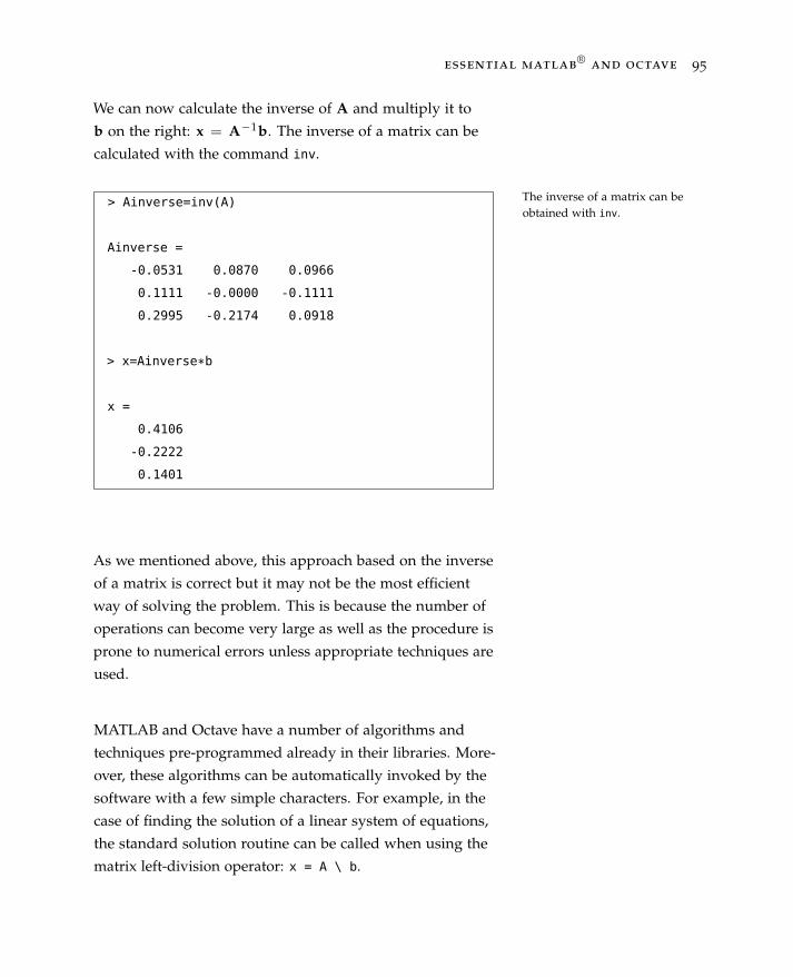
essential matlab®

and octave 95

We can now calculate the inverse of A and multiply it to

b on the right: x = A−1b. The inverse of a matrix can be

calculated with the command inv.

The inverse of a matrix can beobtained with inv.

> Ainverse=inv(A)

Ainverse =

-0.0531 0.0870 0.0966

0.1111 -0.0000 -0.1111

0.2995 -0.2174 0.0918

> x=Ainverse*b

x =

0.4106

-0.2222

0.1401

As we mentioned above, this approach based on the inverse

of a matrix is correct but it may not be the most efficient

way of solving the problem. This is because the number of

operations can become very large as well as the procedure is

prone to numerical errors unless appropriate techniques are

used.

MATLAB and Octave have a number of algorithms and

techniques pre-programmed already in their libraries. More-

over, these algorithms can be automatically invoked by the

software with a few simple characters. For example, in the

case of finding the solution of a linear system of equations,

the standard solution routine can be called when using the

matrix left-division operator: x = A \ b.

96 j. rogel-salazar

> x = A \ b

x =

0.4106

-0.2222

0.1401

The left division operator, \, canbe used to solve linear systems inMATLAB and Octave.

As we can see we have obtained the same solution in both

cases, except that in the second example we did not have to

calculate explicitly the inverse matrix. Instead we relied on

the software libraries to carry out the operations.

3.11 Summary

In this chapter we have covered the use of matrices

in MATLAB and Octave. We have seen how matrices can

be understood as natural extensions of the concept of row

and column vectors. A matrix is thus a collection of column

vectors next to each other, or alternatively a collection of

stacked row vectors. In that sense, the use of the colon

notation (:) to define lists or sequences of numbers can still

be used here. The elements of a matrix can be extracted and

manipulated using the row and column indices in a very

straightforward manner.

We also learned how to carry out important operations on

matrices, such as the transpose with the use of the apostro-

phe or single quote (’) as well as the command transpose.

We also saw how to define special matrices with the aid of

commands such as ones and zeros. Important matrices such

as the identity matrix and diagonal matrices can be easily

constructed with the eye and diag commands.

essential matlab®

and octave 97

Similarly, we also saw how to perform common operations

on matrices such as addition, substraction and multiplica-

tion. In particular we covered two types of multiplication:

the dot-star (.*) product (element-by-element) and the star

product (*) which corresponds to true matrix multiplication.

Finally, we covered the construction of sparse matrices with

the sparse and spdiag commands and used MATLAB and

Octave to solve linear systems of equations.

In the next chapter we will see the powerful visualisation

features that are included in MATLAB and Octave. They

will enable us to analyse and solve problems in a more

integrated manner than many other programming systems.

98 j. rogel-salazar

3.12 Exercises

1. Use MATLAB and Octave to enter the following matrix:

M =

15 9 −i 8

−9 4 0.4 −9.1

1 + i 4 −7 3

4 3.3 9 6.5

.

(a) Create a vector M1 with the elements in the second

row of M.

(b) Create a vector M2 with the elements of the third

column of matrix M.

(c) Create a vector M3 with the elements in the diagonal

of matrix M.

2. Use MATLAB and Octave to enter the following matrix:

M =

4 7 9 0

8 −42 5 −π

4 2 0 1

−6 −5 −4 −3

.

(a) Create a 3 × 4 matrix with the elements of the second

through to fourth columns of M.

(b) Create a 2 × 2 matrix with the elements at the centre of

matrix M.

(c) Create a 2 × 3 matrix with the elements of the first two

columns and last three rows of matrix M.

3. Given the matrices

A =

(10 15

8 6

), B =

(−1 5

0.5 6.3

),

calculate the following:

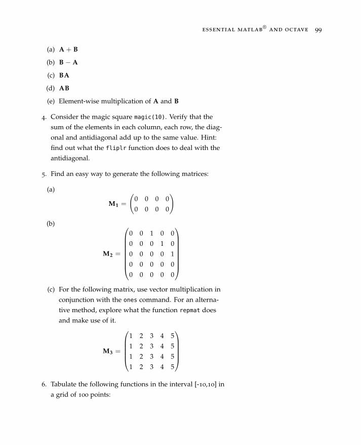
essential matlab®

and octave 99

(a) A + B

(b) B − A

(c) BA

(d) AB

(e) Element-wise multiplication of A and B

4. Consider the magic square magic(10). Verify that the

sum of the elements in each column, each row, the diag-

onal and antidiagonal add up to the same value. Hint:

find out what the fliplr function does to deal with the

antidiagonal.

5. Find an easy way to generate the following matrices:

(a)

M1 =

(0 0 0 0

0 0 0 0

)

(b)

M2 =

0 0 1 0 0

0 0 0 1 0

0 0 0 0 1

0 0 0 0 0

0 0 0 0 0

(c) For the following matrix, use vector multiplication in

conjunction with the ones command. For an alterna-

tive method, explore what the function repmat does

and make use of it.

M3 =

1 2 3 4 5

1 2 3 4 5

1 2 3 4 5

1 2 3 4 5

6. Tabulate the following functions in the interval [-10,10] in

a grid of 100 points:

100 j. rogel-salazar

(a) y = ln(x2) + 1

(b) y = 1x+72

(c) y = 3 exp(−x2)

7. Find out what the functions randn and reshape do. Use

one of the functions to create a 10 × 10 matrix with

random elements. Find the maximum values in each

column, each row and overall with the help of the max

function. Use the other function to transform the 10 × 10

matrix into a 25 × 4 matrix.

8. Create a sparse matrix such that

A =

(1 aT

a In

),

where a is an n × n matrix, 1 is a matrix of ones and In

is an n × n identity matrix. If a is a matrix with random

elements, with n = 100, create the corresponding matrix

A and visualise its structure.

9. Consider the matrix

B =

2 1 −1

1 2 1

1 1 2

.

Using the command eig find the eigenvalues and eigen-

vectors of B, BT and B−1. What relationship (if any) is

there between your results.

Do the same for the matrix B1 below. What do the eigen-

values tell you about the matrix?

B1 =

2 1 −1

1 2 1

1 1 0

essential matlab®

and octave 101

10. Using MATLAB and Octave, solve the following linear

systems of equations:

(a)

2w − x + 5y + z = 3

3w + 2x + 2y − 6z = −32

5w − 2x − 3y + 3x = 49

w + 3x + 3y − z = −47

(b)

x1 + x2 + x3 = 4

−3x1 + 2x2 − 5x3 = −14

2x1 − 3x2 + 4x3 = 10

103

4

Plotting

We are now familiar with some of the most essential

elements of MATLAB® and Octave, namely, vectors and

matrices. We have learned how to manipulate them and

carry out important operations with them such as addition,

substraction, multiplication and, within the definition in the

software, even division. Similarly, we know how to address

and extract individual elements as well as sequences of

elements.

In this chapter we turn our attention to one of the distin-

guishing features of MATLAB and Octave, i.e. the plotting

and visualisation capabilities integrated with the devel-

opment environment itself. Whereas other programming

environments do not include a way to produce plots and

graphs, MATLAB and Octave enable us to merge data visu-

alisation directly to our workflow.

MATLAB and Octave integratedata visualisation directly to theprogramming environment.

4.1 Plotting Simple Functions

We have had a look at how to enter and evaluate a

number of expressions and built-in functions in MATLAB

104 j. rogel-salazar

and Octave. In this chapter we are going to see how to

visualise those expressions in the form of plots.

Let us consider the function

y(x) = cos(4x), (4.1)

and imagine that we are interested in creating a graph of

this function in the interval 0 ≤ x ≤ π. This can be easily

done by

• taking a sample of points,

• evaluating the function at those points and

• joining the calculated values with appropriate lines.

A common and simple approach is to take equally spaced

points along the x values. We can thus have n + 1 points a

distance h apart from each other; for example, in the case of

n = 20 we can write:

> n = 20;

> h = pi/n;

> x = 0:h:pi;

Setting up an equally spacedvector of points.

This will therefore create a set of points stored in the vari-

able x. We could also use the command linspace, whose

format is

linspace(a,b,n)

Equidistant-element vectors canalso be created with the linspace

command.

which generates a vector with n points at an equal distance

from each other between the values a and b. So for the case

above we can write

essential matlab®

and octave 105

> x = linspace(0,pi,21);

It is now possible to evaluate y at the various points given

by the values stored in the vector x:

> y = cos(4*x);

Finally the plot of the points calculated above can be ob-

tained by using the plot command

> plot(x,y)The plot command can be used toproduce graphs.

The result of the commands above is shown in Figure 4.1,

where it is clear that the number of points used is small

given the jagged profile obtained.

The jagged result can easily be improved upon by increasing

the number of points to, for instance, 200:

> N = 199;

Note that we need to specify N − 1 so that the colon notation

generates a vector with N elements. All we need to do now

is repeat the calculations and recreate the plot with the

increased number of points:

> h = pi/N;

> x = 0:h:pi;

> y = cos(4*x);

> plot(x,y)

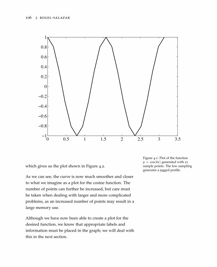
106 j. rogel-salazar

0 0.5 1 1.5 2 2.5 3 3.5ï1

ï0.8

ï0.6

ï0.4

ï0.2

0

0.2

0.4

0.6

0.8

1

Figure 4.1: Plot of the functiony = cos(4x) generated with 21

sample points. The low samplinggenerates a jagged profile.

which gives us the plot shown in Figure 4.2.

As we can see, the curve is now much smoother and closer

to what we imagine as a plot for the cosine function. The

number of points can further be increased, but care must

be taken when dealing with larger and more complicated

problems, as an increased number of points may result in a

large memory use.

Although we have now been able to create a plot for the

desired function, we know that appropriate labels and

information must be placed in the graph; we will deal with

this in the next section.

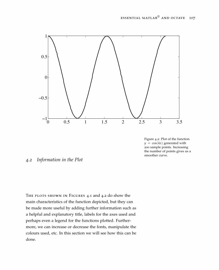
essential matlab®

and octave 107

0 0.5 1 1.5 2 2.5 3 3.5ï1

ï0.5

0

0.5

1

Figure 4.2: Plot of the functiony = cos(4x) generated with200 sample points. Increasingthe number of points gives us asmoother curve.

4.2 Information in the Plot

The plots shown in Figures 4.1 and 4.2 do show the

main characteristics of the function depicted, but they can

be made more useful by adding further information such as

a helpful and explanatory title, labels for the axes used and

perhaps even a legend for the functions plotted. Further-

more, we can increase or decrease the fonts, manipulate the

colours used, etc. In this section we will see how this can be

done.

108 j. rogel-salazar

4.2.1 Titles and Labels

It is very useful to add a title that describes the plot as

well as information about what it is that is being plotted

along each of the axes. In order to add a title and label

the axes in the plot, we use the commands title, xlabel

and ylabel. Try out the following commands for the plot

generated in the previous section; the result can be seen in

Figure 4.3.

> title(’Graph of y = cos(4 x)’)

> xlabel(’x-axis’)

> ylabel(’y-axis’)

The commands title, xlabel andylabel let us add a title to the plotand label its axes.

The strings enclosed in single quotes can be (almost) any-

thing we choose. Some simple LATEX commands are avail-

able for formatting mathematical expressions and Greek

characters. More information about this can be seen in

Section 4.6.

The text included in the title andlabels supports the use of someLATEX commands.

4.2.2 Grids

Sometimes it is useful to show a grid that helps guide

the eye when looking at a plot. For example, a dotted grid

may be added by issuing the following command:

> grid

In cases where this is not required, the grid can be removed

using either grid again, or grid off.

The command grid enables adotted grid to be shown in a plot.

essential matlab®

and octave 109

0 0.5 1 1.5 2 2.5 3 3.5ï1

ï0.8

ï0.6

ï0.4

ï0.2

0

0.2

0.4

0.6

0.8

1Graph of y = cos(4 x)

xïaxis

yïax

is

Figure 4.3: Plot of the functiony = cos(4x) including a title andlabels for each axis.4.2.3 Line Styles and Colours

When creating a plot, the default is to present the graph

with a blue solid line. A more general command to create a

plot specifying a solid blue line is as follows:

A more general form for the plot

command specifies the colour andtype of line to be used.

> plot(x,y,’b-’)

From the discussion in the previous sections we know the

meaning of the first two arguments passed to the plot com-

mand. This leaves us with the third argument, which is a

string (we know this because it is enclosed in single quo-

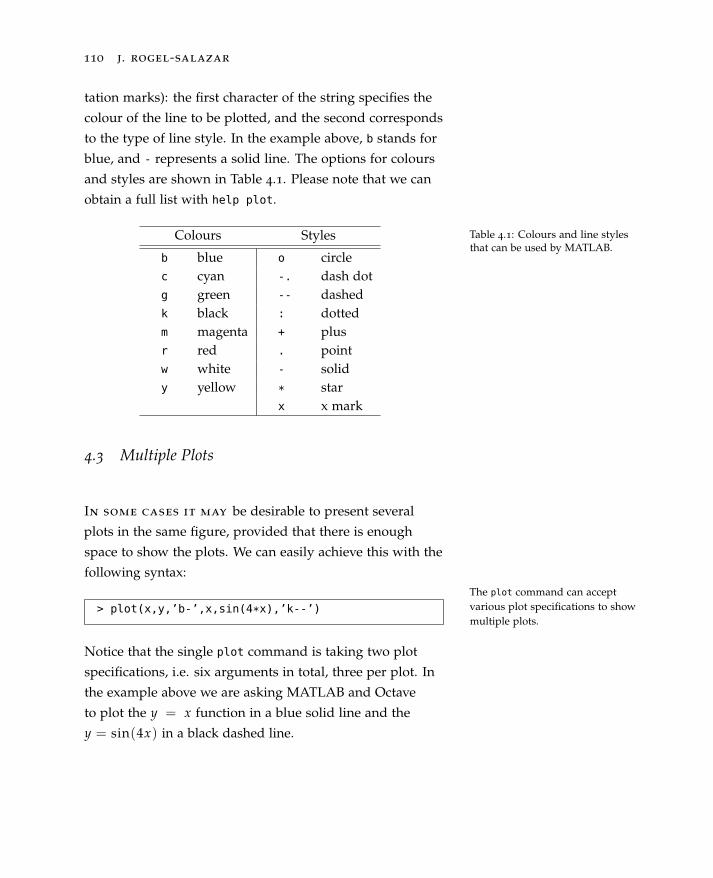
110 j. rogel-salazar

tation marks): the first character of the string specifies the

colour of the line to be plotted, and the second corresponds

to the type of line style. In the example above, b stands for

blue, and - represents a solid line. The options for colours

and styles are shown in Table 4.1. Please note that we can

obtain a full list with help plot.

Colours Styles

b blue o circlec cyan -. dash dotg green -- dashedk black : dottedm magenta + plusr red . pointw white - solidy yellow * star

x x mark

Table 4.1: Colours and line stylesthat can be used by MATLAB.

4.3 Multiple Plots

In some cases it may be desirable to present several

plots in the same figure, provided that there is enough

space to show the plots. We can easily achieve this with the

following syntax:The plot command can acceptvarious plot specifications to showmultiple plots.

> plot(x,y,’b-’,x,sin(4*x),’k--’)

Notice that the single plot command is taking two plot

specifications, i.e. six arguments in total, three per plot. In

the example above we are asking MATLAB and Octave

to plot the y = x function in a blue solid line and the

y = sin(4x) in a black dashed line.

essential matlab®

and octave 111

In cases like the one above it is highly recommended to

include a legend that lets the reader know what is being

plotted. This can be done by using:

We can add a legend to the plotwith the legend command.

> legend(’cos(4x)’,’sin(4x)’)

The result of the command above will provide a list of line-

styles, as they appeared in the plot command, followed

by a brief description (the strings passed to the legend

command).

The final output of the commands used above (including

a title, labels and grid) can be seen in Figure 4.4. Please

note that the figure created by MATLAB and Octave in

the screen will have the graph for the cos(4x) in blue; the

figure shown here is printed in black and white.

4.4 Holding Figures

Every time that the we create a graph with the plot

command, MATLAB and Octave clear the contents of the

current figure. In a lot of cases this is perfectly fine, however

if we are interested in adding other plots to the same figure

we can instruct the software to keep the current contents

with the hold function. The command can be turned on or

off as follows:

The current figure can be heldwith the hold command to con-tinue adding plots to it.

> plot(x,cos(4*x),’k-’), hold on

> plot(x,sin(4*x),’b--’), hold off

The command hold on keeps the current picture whereas

hold off releases it (but does not clear the window, which

can be done with clf). Let us see what the above instruc-

To clear the window we can usethe clf command.

112 j. rogel-salazar

0 0.5 1 1.5 2 2.5 3 3.5ï1

ï0.5

0

0.5

1

xïaxis

yïax

isMultiple Plots in a Figure

cos(4x)sin(4x)

Figure 4.4: Multiple plots in thesame figure can be placed usingthe plot command.tions do: first we are asking the software to plot the vector

that holds the values of the function

y1 = cos(4x) (4.2)

against the values held by the vector x; the plot is done

using a black solid line and we hold the figure for further

plotting.

We then request the plot of the function

y2 = sin(x) (4.3)

against the values of the vector x using a blue dashed line.

Since we asked for the figure to be held, the second plot will

essential matlab®

and octave 113

be placed in the same frame as the previous one. Finally,

we instruct MATLAB and Octave to free the plot with the

command hold off. The result of the commands above can

be seen in Figure 4.4, which shows the plots printed in black

and white.

4.5 Subplots

In the previous section we have seen how to add plots to

the same figure window in a frame. However, in some cases

we may prefer to split the graphics window to show plots in

separate frames. We can do this by dividing the figure into

an m × n array of smaller windows into which we may plot

one or more graphs.

The sub-windows are counted 1 to mn row by row starting

from the top left. Both hold and grid work on the current Subplots are enumerated by rowfrom the top left.subplot and so these commands must be used as the rele-

vant plots are being produced.

The arrangement of subplots can be created with the

subplot(m,n,number), where m and n define the plot ar- An arrangement of subplots isachieved with the commandsubplot(m,n,number).

ray and number is the label of the relevant subplot to use.

For example, take a look at the following code:

> subplot(2,2,1)

> plot(x,cos(4*x))

> title(’y=cos(4 x)’)

> xlabel(’x’), ylabel(’cos(4 x)’)

The command subplot(2,2,1) specifies that the window

should be split into a 2 × 2 array and we select the first sub-

window, where the function y = cos(4x) is being plotted

using the default colour and line style.

114 j. rogel-salazar

We can continue filling in the rest of the other three subplots

by issuing commands similar to the ones above while speci-

fying the relevant number to refer to the correct frame where

we want the graphs to be plotted. Look at the following

commands:

> subplot(2,2,2)

> plot(x,sin(4*x))

> title(’y=sin(4 x)’)

> xlabel(’x’), ylabel(’sin(4 x)’)

which will generate the second plot; for the third one we

The subplot command requiresus to tell it what subfigure in thearray to use for plotting.

have:

> subplot(2,2,3)

> plot(x, x)

> title(’y=x’)

> xlabel(’x’), ylabel(’y’)

and finally, for the fourth one:

> subplot(2,2,4)

> plot(x,x.^2)

> title(’y=x^2’)

> xlabel(’x’),ylabel(’y’)

Notice that with each subplot command we specify what

sub-window to use; for instance in the first case we have

asked MATLAB and Octave to plot the function y = sin(4x)in the top right sub-window of the arrangement. Similar

specifications have been made for the plots of y = x and

y = x2 in the lower left- and lower right-hand corners of the

main figure.

Each subplot can be identifiedwith the index associated with it.

After plotting each of the subfigures we have issued com-

mands to add appropriate labels to the axes. That is because

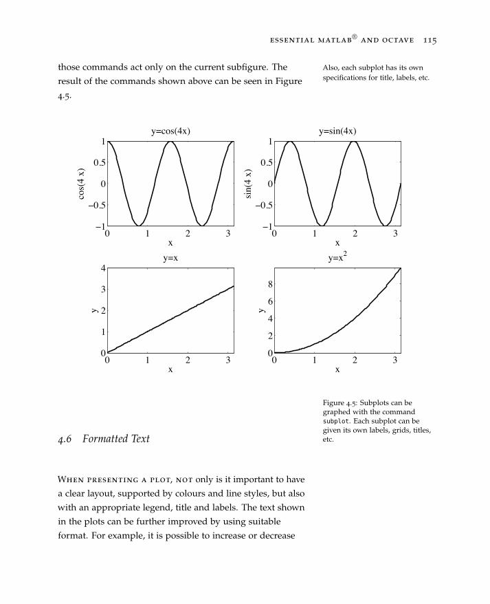
essential matlab®

and octave 115

those commands act only on the current subfigure. The Also, each subplot has its ownspecifications for title, labels, etc.result of the commands shown above can be seen in Figure

4.5.

0 1 2 3ï1

ï0.5

0

0.5

1y=cos(4x)

x

cos(

4 x)

0 1 2 3ï1

ï0.5

0

0.5

1y=sin(4x)

xsi

n(4

x)

0 1 2 30

1

2

3

4y=x

x

y

0 1 2 30

2

4

6

8

y=x2

x

y

Figure 4.5: Subplots can begraphed with the commandsubplot. Each subplot can begiven its own labels, grids, titles,etc.4.6 Formatted Text

When presenting a plot, not only is it important to have

a clear layout, supported by colours and line styles, but also

with an appropriate legend, title and labels. The text shown

in the plots can be further improved by using suitable

format. For example, it is possible to increase or decrease

116 j. rogel-salazar

the size of the text as well as add simple mathematical

expressions (in LATEX form).

MATLAB and Octave acceptsimple LATEX commands to formattext.

Let us take a look at an example by plotting in a panel the

first 20 terms of the following sequence:

xn =n2 + 7

n2 , (4.4)

and then, in a second panel, plot the function

y1 = π cos2(4x) (4.5)

on the interval −1 ≤ x ≤ 1, finally adding some formatted

text to the figure we are putting together. The tasks men-

tioned above can be achieved in MATLAB and Octave as

follows.

In order to provide text that is readable, we can start by

setting the default font size for the axis labels, legends and

titles to a size of 16 points. In order to do that we can use

the command set as follows:

> set(0,’Defaultaxesfontsize’,16); We can change the default fontsize.

The first argument issued above refers to the current figure,

whereas the second one in this case tells the software what

property we are changing, and finally we provide the new

size for the font.

We can now define the series given by Equation (4.4). Since

we are interested in the first 20 terms, we can define a vector

containing the sequence of numbers from 1 to 20 and use

that to calculate the series:

essential matlab®

and octave 117

> n = 1:20;

> x = (n.^2+7)./n.^2;

This particular sequence converges to the value of 1, and we

would like to show this in the plot we are going to create.

In the first panel we are therefore going to plot each of the

20 terms of the sequence marked by blue dots, and add a

horizontal green dotted line to show the convergence of the

sequence: The plot command is used to graph the sequence

stored in the vector x versus the term number held in the

vector n. In order to show the horizontal line, we create on

the fly a couple of 2-element vectors whose values provide

the information needed to plot the line. Finally, in the same

plot command we use markersize to change the default

value (6) of the marker size to the value of 10.

The markersize property can beused to change the size of themarkers in a plot.

> subplot (2,1,1)

> plot(n,x,’.’,...

[0 max(n)],[1 1],’--’,’markersize’,10);

Remember that the commands to add titles, labels and

legends act only on the current figure. We add a title to the

subplot, changing the size of the font to 20 using fontsize.

The fontsize property changedthe size of the fonts used in a plot.

Similarly, we add labels and a legend. Notice that we can

indicate to MATLAB and Octave the location of the legend

with the aid of a second argument, where 1 stands for

upper-right-hand corner, 2 is upper-left-hand corner, 3 is the

lower-left-hand corner and 4 is the lower-right-hand corner.

The position of the legend canbe specified with the help of thesecond argument passed on to thecommand legend.

MATLAB and Octave are able to understand some simple

syntax used in LATEX to generate mathematical formulae

such as _, ^, \alpha, \pi, \sin, \cos, etc.

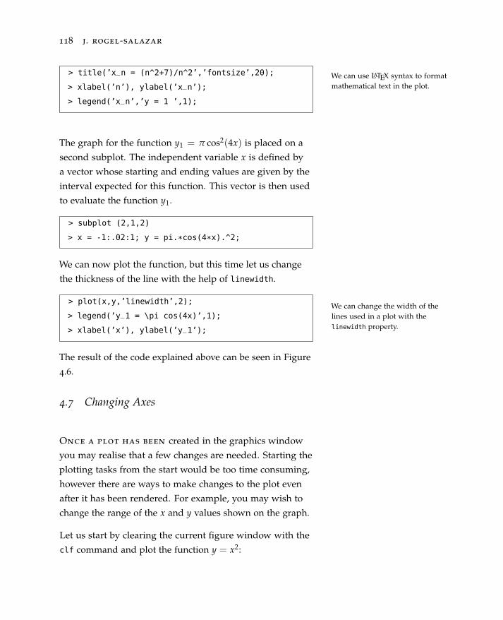
118 j. rogel-salazar

> title(’x_n = (n^2+7)/n^2’,’fontsize’,20);

> xlabel(’n’), ylabel(’x_n’);

> legend(’x_n’,’y = 1 ’,1);

We can use LATEX syntax to formatmathematical text in the plot.

The graph for the function y1 = π cos2(4x) is placed on a

second subplot. The independent variable x is defined by

a vector whose starting and ending values are given by the

interval expected for this function. This vector is then used

to evaluate the function y1.

> subplot (2,1,2)

> x = -1:.02:1; y = pi.*cos(4*x).^2;

We can now plot the function, but this time let us change

the thickness of the line with the help of linewidth.

We can change the width of thelines used in a plot with thelinewidth property.

> plot(x,y,’linewidth’,2);

> legend(’y_1 = \pi cos(4x)’,1);

> xlabel(’x’), ylabel(’y_1’);

The result of the code explained above can be seen in Figure

4.6.

4.7 Changing Axes

Once a plot has been created in the graphics window

you may realise that a few changes are needed. Starting the

plotting tasks from the start would be too time consuming,

however there are ways to make changes to the plot even

after it has been rendered. For example, you may wish to

change the range of the x and y values shown on the graph.

Let us start by clearing the current figure window with the

clf command and plot the function y = x2:

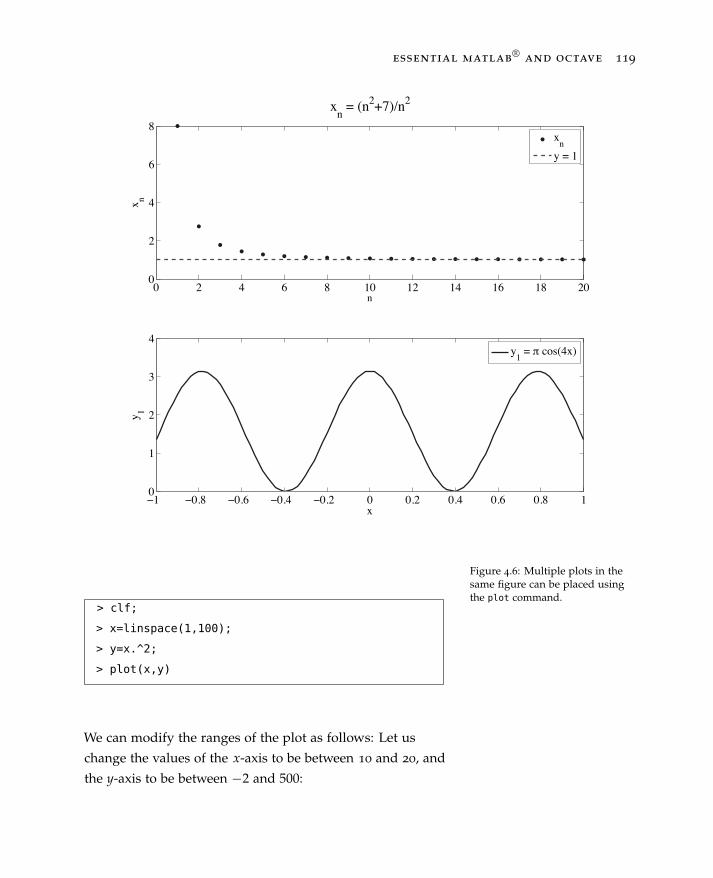
essential matlab®

and octave 119

0 2 4 6 8 10 12 14 16 18 200

2

4

6

8

xn = (n2+7)/n2

n

x n

xny = 1

ï1 ï0.8 ï0.6 ï0.4 ï0.2 0 0.2 0.4 0.6 0.8 10

1

2

3

4

x

y 1

y1 = / cos(4x)

Figure 4.6: Multiple plots in thesame figure can be placed usingthe plot command.

> clf;

> x=linspace(1,100);

> y=x.^2;

> plot(x,y)

We can modify the ranges of the plot as follows: Let us

change the values of the x-axis to be between 10 and 20, and

the y-axis to be between −2 and 500:

120 j. rogel-salazar

> axis([10 20 -2 500])

The axis command has four parameters: the first two are

The axis command enables us tochange the ranges of the values inthe plot.

the minimum and maximum values to be used for the

x-axis and the last two are the minimum and maximum

values for the y-axis. In order to compare the changes let us

enter the following commands in the software:

> clf;

> x=linspace(1,100);

> y=x.^2;

> subplot(1,2,1)

> plot(x,y)

> title(’y=x^2 with default axes’)

> xlabel(’x’), ylabel(’y’)

> subplot(1,2,2)

> plot(x,y)

> axis([10 20 -2 500])

> title(’y=x^2 with custom axes’)

> xlabel(’x’), ylabel(’y’)

The result of these commands is shown in Figure 4.7. We

recommend taking a look at help axis as well as the infor-

mation on the following:

• axis equal: the aspect ratio is set such that the data units

are the same in each direction;

• axis square: makes the axes have equal lengths;

• axis normal: the aspect ratio is adjusted to fit the space

in the figure;

• axis tight: sets the axes to the range of the data.

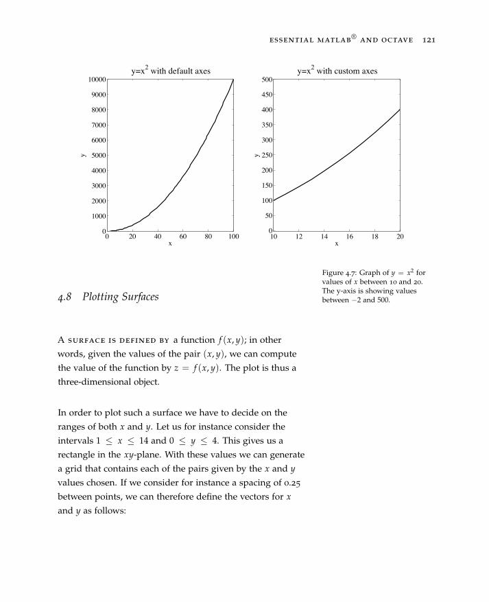
essential matlab®

and octave 121

0 20 40 60 80 1000

1000

2000

3000

4000

5000

6000

7000

8000

9000

10000y=x2 with default axes

x

y

10 12 14 16 18 200

50

100

150

200

250

300

350

400

450

500y=x2 with custom axes

xy

Figure 4.7: Graph of y = x2 forvalues of x between 10 and 20.The y-axis is showing valuesbetween −2 and 500.4.8 Plotting Surfaces

A surface is defined by a function f (x, y); in other

words, given the values of the pair (x, y), we can compute

the value of the function by z = f (x, y). The plot is thus a

three-dimensional object.

In order to plot such a surface we have to decide on the

ranges of both x and y. Let us for instance consider the

intervals 1 ≤ x ≤ 14 and 0 ≤ y ≤ 4. This gives us a

rectangle in the xy-plane. With these values we can generate

a grid that contains each of the pairs given by the x and yvalues chosen. If we consider for instance a spacing of 0.25

between points, we can therefore define the vectors for xand y as follows:

122 j. rogel-salazar

> x = 1:0.25:14;

> y = 0:0.25:4;

The vectors above provide us with the length of each side of

the square in the xy-plane, but we need to define the points

that map that plane, i.e. a grid.

The grid can be defined in MATLAB and Octave with the

command meshgrid, and the values obtained can be used toThe points used to define a plotsurface can be calculated with themeshgrid command.

get the coordinates of the point (X(i, j), Y(i, j)) using the

i−th point along from the left and the j−th point up from

the bottom of the grid which correspond to the (i, j) entry

in a matrix. The command meshgrid takes two vectors, x

and y, that define each side of a rectangular grid resulting

in a mesh of values that define the points inside it. Here is

how:

The meshgrid command generatedthe points inside a rectangulargrid which in turn can be used todefine a surface.

> [X,Y] = meshgrid(x,y)

X =

1.000 1.250 1.500 1.750 2.000 ...

1.000 1.250 1.500 1.750 2.000 ...

1.000 1.250 1.500 1.750 2.000 ...

1.000 1.250 1.500 1.750 2.000 ...

1.000 1.250 1.500 1.750 2.000 ...

1.000 1.250 1.500 1.750 2.000 ...

...

Y =

0 0 0 0 0 ...

0.250 0.250 0.250 0.250 0.250 ...

0.500 0.500 0.500 0.500 0.500 ...

0.750 0.750 0.750 0.750 0.750 ...

1.000 1.000 1.000 1.000 1.000 ...

1.250 1.150 1.250 1.250 1.250 ...

...

essential matlab®

and octave 123

Please note that we have truncated the output shown above.

In this particular case, the arrays X and Y are (17 × 53)-

matrices and showing them here would not be very practi-

cal.

Finally, the values of the matrices X and Y can now be used

to evaluate the function f (x, y). Let us consider for instance

the function

f (x, y) = sin(x − 1) + cos(3y − 1) (4.6)

for the ranges we had decided upon. The plot can be cre-

ated in MATLAB and Octave with the surfl command:

> Z = sin(X-1)+cos(3*Y-1);

> surfl(X,Y,Z)

> colormap(gray)

> title(’A surface’)

> xlabel(’x’)

> ylabel(’y’)

> zlabel(’z’)

> grid on

The surfl command is used tocreate a surface plot.

The result can be seen in Figure 4.8. Notice that we used the

command colormap to provide a colour scale to be used in

The command colormap providesus with colour scales to be used inthe surface plot.

the plot; some common colour maps in the software include:

• Jet: ranges from blue to red

• HSV: from red to red passing through yellow, green,

cyan, blue, magenta

• Hot: from black to white passing through red, orange

and yellow

• Cool: from cyan to magenta

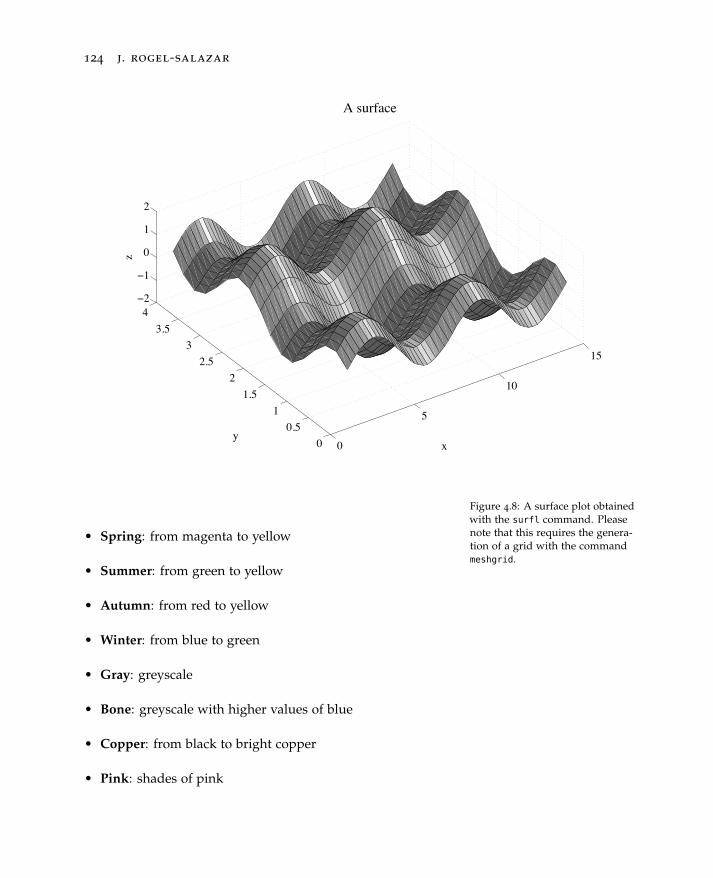
124 j. rogel-salazar

0

5

10

15

00.5

11.5

22.5

33.5

4ï2

ï1

0

1

2

x

A surface

y

z

Figure 4.8: A surface plot obtainedwith the surfl command. Pleasenote that this requires the genera-tion of a grid with the commandmeshgrid.

• Spring: from magenta to yellow

• Summer: from green to yellow

• Autumn: from red to yellow

• Winter: from blue to green

• Gray: greyscale

• Bone: greyscale with higher values of blue

• Copper: from black to bright copper

• Pink: shades of pink

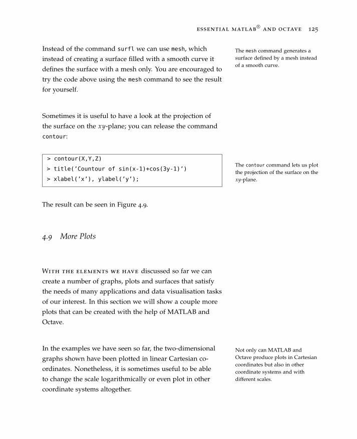
essential matlab®

and octave 125

Instead of the command surfl we can use mesh, which

instead of creating a surface filled with a smooth curve it

defines the surface with a mesh only. You are encouraged to

The mesh command generates asurface defined by a mesh insteadof a smooth curve.

try the code above using the mesh command to see the result

for yourself.

Sometimes it is useful to have a look at the projection of

the surface on the xy-plane; you can release the command

contour:

The contour command lets us plotthe projection of the surface on thexy-plane.

> contour(X,Y,Z)

> title(’Countour of sin(x-1)+cos(3y-1)’)

> xlabel(’x’), ylabel(’y’);

The result can be seen in Figure 4.9.

4.9 More Plots

With the elements we have discussed so far we can

create a number of graphs, plots and surfaces that satisfy

the needs of many applications and data visualisation tasks

of our interest. In this section we will show a couple more

plots that can be created with the help of MATLAB and

Octave.

In the examples we have seen so far, the two-dimensional

graphs shown have been plotted in linear Cartesian co-

ordinates. Nonetheless, it is sometimes useful to be able

to change the scale logarithmically or even plot in other

coordinate systems altogether.

Not only can MATLAB andOctave produce plots in Cartesiancoordinates but also in othercoordinate systems and withdifferent scales.

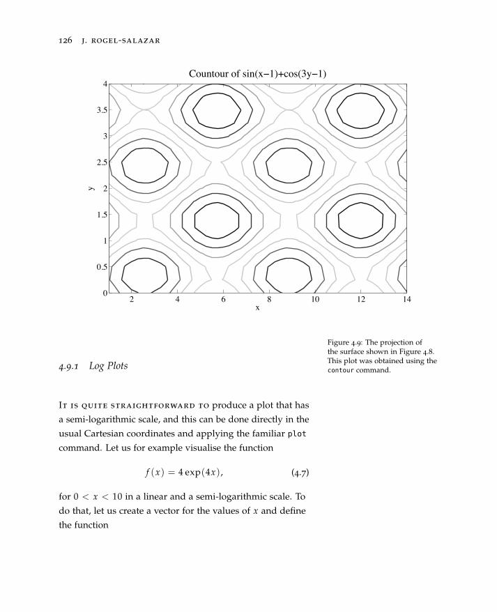
126 j. rogel-salazar

Countour of sin(xï1)+cos(3yï1)

x

y

2 4 6 8 10 12 140

0.5

1

1.5

2

2.5

3

3.5

4

Figure 4.9: The projection ofthe surface shown in Figure 4.8.This plot was obtained using thecontour command.4.9.1 Log Plots

It is quite straightforward to produce a plot that has

a semi-logarithmic scale, and this can be done directly in the

usual Cartesian coordinates and applying the familiar plot

command. Let us for example visualise the function

f (x) = 4 exp(4x), (4.7)

for 0 < x < 10 in a linear and a semi-logarithmic scale. To

do that, let us create a vector for the values of x and define

the function

essential matlab®

and octave 127

> x = linspace(1,10);

> y = 4*exp(2*x);

In order to compare the two scales, we will use the subplot

command to create an array of two graphs, one on top of

the other:

> subplot(2,1,1);

> plot(x,y,’k’,’LineWidth’,2);

> title(’y=4 exp(2x) with linear axes’)

> xlabel(’x’), ylabel(’y’)

> subplot(2,1,2);

> semilogy(x,y,’k’,’LineWidth’,2);

> title(’y=4 exp(2x) with semilog axes’)

> xlabel(’x’), ylabel(’y’)

We can use the semilogy com-mand to create plots in a semi-logarithmic scale.

The commands above are quite familiar to us, except for

semilogy. Nonetheless, it is very easy to figure out what

it does: it plots a graph in a semi-logarithmic scale. The

output of the commands can be seen in Figure 4.10 and it

is very easy to corroborate that in a semi-logarithmic graph,

the function is represented as a straight line as shown in the

bottom panel of the figure.

As we can see, in the top panel of Figure 4.10 it is quite

difficult to see what is going on in the interval from 0 to 7.

This is because the values are quite small. Nonetheless, by

using the logarithmic scale, as shown in the bottom panel of

Figure 4.10, it becomes much more obvious what is going

on in that interval.

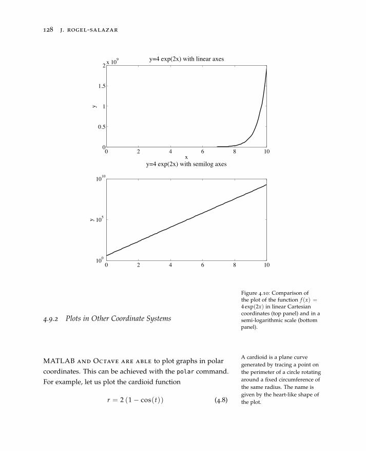
128 j. rogel-salazar

0 2 4 6 8 100

0.5

1

1.5

2 x 109 y=4 exp(2x) with linear axes

x

y

0 2 4 6 8 10100

105

1010

y=4 exp(2x) with semilog axes

y

Figure 4.10: Comparison ofthe plot of the function f (x) =4 exp(2x) in linear Cartesiancoordinates (top panel) and in asemi-logarithmic scale (bottompanel).

4.9.2 Plots in Other Coordinate Systems

MATLAB and Octave are able to plot graphs in polar

coordinates. This can be achieved with the polar command.

For example, let us plot the cardioid function

A cardioid is a plane curvegenerated by tracing a point onthe perimeter of a circle rotatingaround a fixed circumference ofthe same radius. The name isgiven by the heart-like shape ofthe plot.r = 2 (1 − cos(t)) (4.8)

essential matlab®

and octave 129

for values of t ∈ [0, 2π ]. To do this, we will define a vector

that contains the values of t and use them to create the plot

as follows:

We can plot the cardioid with thepolar command.

> t=0:0.01:2*pi;

> polar(t,2*(1-cos(t)))

The plot is effectively a curve described in the complex

plane and the result of the commands above can be seen

in Figure 4.11 where we are showing the output as pro-

duced by MATLAB; Octave will produce a similar, although

simpler, graphic than the one shown here.

An alternative way to produce the plot is to generate the

values of the cardioid function, but instead of creating

the plot in polar coordinates we can find the appropriate

transformation of these values into Cartesian coordinates.

Let us take a look at how to achieve this. First we define the

cardioid curve as follows:

> t=0:0.01:2*pi;

> r = 2*(1-cos(t));

We can now use the pol2cart command in order to find

the Cartesian coordinates that correspond to the polar ones. The command port2cart findsthe transformation from polar toCartesian coordinates.

The input for this command is the angular (t) and radial (r)

coordinates and the output is the familiar x and y Cartesian

coordinates.

> [x, y] = pol2cart(t,r);

> plot(x,y);

Once the coordinate transformation has been carried out, we

can use the command plot to visualise the graph and the

result can be seen in Figure 4.12

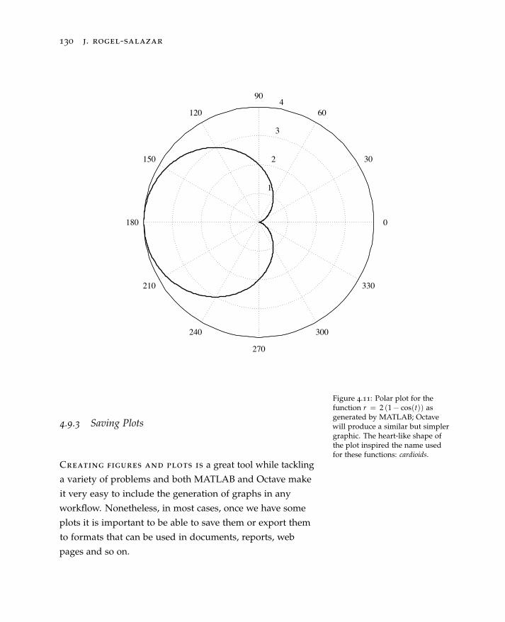
130 j. rogel-salazar

1

2

3

4

30

210

60

240

90

270

120

300

150

330

180 0

Figure 4.11: Polar plot for thefunction r = 2 (1− cos(t)) asgenerated by MATLAB; Octavewill produce a similar but simplergraphic. The heart-like shape ofthe plot inspired the name usedfor these functions: cardioids.

4.9.3 Saving Plots

Creating figures and plots is a great tool while tackling

a variety of problems and both MATLAB and Octave make

it very easy to include the generation of graphs in any

workflow. Nonetheless, in most cases, once we have some

plots it is important to be able to save them or export them

to formats that can be used in documents, reports, web

pages and so on.

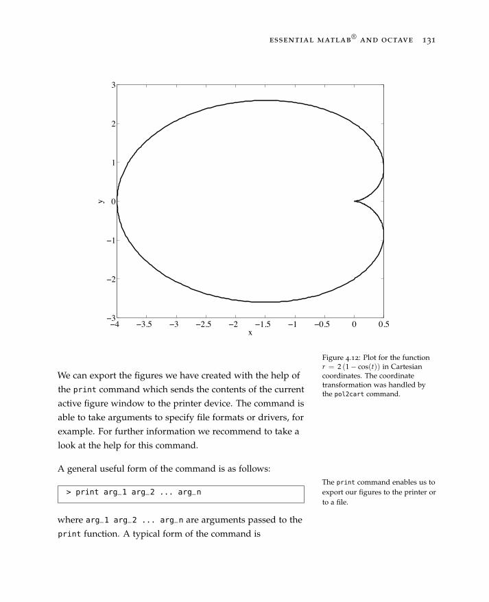
essential matlab®

and octave 131

ï4 ï3.5 ï3 ï2.5 ï2 ï1.5 ï1 ï0.5 0 0.5ï3

ï2

ï1

0

1

2

3

x

y

Figure 4.12: Plot for the functionr = 2 (1− cos(t)) in Cartesiancoordinates. The coordinatetransformation was handled bythe pol2cart command.

We can export the figures we have created with the help of

the print command which sends the contents of the current

active figure window to the printer device. The command is

able to take arguments to specify file formats or drivers, for

example. For further information we recommend to take a

look at the help for this command.

A general useful form of the command is as follows:The print command enables us toexport our figures to the printer orto a file.

> print arg_1 arg_2 ... arg_n

where arg_1 arg_2 ... arg_n are arguments passed to the

print function. A typical form of the command is

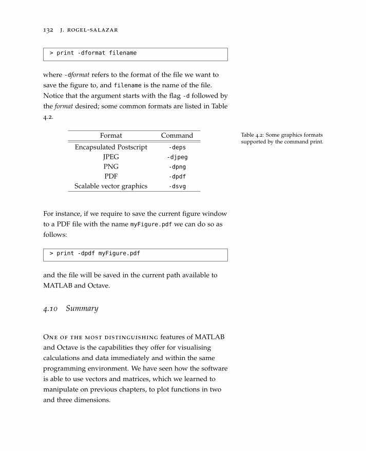
132 j. rogel-salazar

> print -dformat filename

where -dformat refers to the format of the file we want to

save the figure to, and filename is the name of the file.

Notice that the argument starts with the flag -d followed by

the format desired; some common formats are listed in Table

4.2.

Format Command

Encapsulated Postscript -deps

JPEG -djpeg

PNG -dpng

PDF -dpdf

Scalable vector graphics -dsvg

Table 4.2: Some graphics formatssupported by the command print.

For instance, if we require to save the current figure window

to a PDF file with the name myFigure.pdf we can do so as

follows:

> print -dpdf myFigure.pdf

and the file will be saved in the current path available to

MATLAB and Octave.

4.10 Summary

One of the most distinguishing features of MATLAB

and Octave is the capabilities they offer for visualising

calculations and data immediately and within the same

programming environment. We have seen how the software

is able to use vectors and matrices, which we learned to

manipulate on previous chapters, to plot functions in two

and three dimensions.

essential matlab®

and octave 133

The plot command lets us visualise the graphs of functions

in two dimensions and is able to take multiple parameters

to enable the visualisation of multiple graphs in one single

figure. In order to render three-dimensional surfaces we

can use the surfl and mesh commands in combination with

the meshgrid command. Furthermore, several plots can be

combined in a figure with the help of subplot.

Not only are we able to visualise data, but we can also add

relevant and important information with the help of format-

ted text for titles, labels and annotations. This information

can be made clearer with the capabilities that MATLAB and

Octave have to process simple LATEX commands. Finally, we

have also seen how to change markers, font sizes, colours

and line widths with the help of relevant parameters as well

as saving our figures in different formats.

In the next chapter we will see how MATLAB and Octave

combine the features we have discussed so far with scripting

capabilities that allow us to explore data and models in a

programmatical manner.

134 j. rogel-salazar

4.11 Exercises

1. Plot the function

f (x) =(6 + x2)

5 + 3x2 , −4 ≤ x ≤ 5.

2. Plot the function

y = exp(−x2

)sin(πx3), −2 ≤ x ≤ 2.

Provide a title and appropriate labels.

3. Plot the following functions in the same window for

values between −2π and 2π. Make sure you include a

legend and title, as well as labels for the axes. Each plot

should have a different colour.

(a) y1 = 3 cos(x)

(b) y2 = −2 cos(2x)

(c) y3 = −0.8 sin(x2)

4. Using the polar command, create a figure with the

following subplots with t ∈ [0, 2π ]:

(a) r1 = et/2

(b) r2 = 2 sin2(t) + 2 cos2(t)

(c) r3 = 0.01t2 − 9.02

(d) r4 = cos(2t)

Compare the plots with those in Cartesian coordinates.

Hint: Use pol2cart.

5. Create the surface and contour plots for the function

z = 2x2 − 2xy + 6y2 ,

for x ∈ [−25, 25] and y ∈ [−20, 20]

essential matlab®

and octave 135

6. Plot the function shown below, including a formatted

legend, labels and title:

f (x) = sin(π

2x)+ sin

(25

πx)

, x ∈ [−3π , 3π ].

7. Create the surface for the function

f (x, y) = (x2 − y2) exp(−x2 − y2)

for x and y in the range [−3, 3].

8. Consider the set of parametric equations:

X = 1.5 cos 4t, Y = 2 sin 5t.

Create the following plots:

(a) X versus t

(b) Y versus t

(c) Y versus X

(d) Find out about the built-in function comet and use it to

animate the Y versus X plot.

9. Plot the following functions in rectangular, semilog and

log-log scales, with x ∈ [0, 3]:

(a) x

(b) x2

(c) e2

(d) ex2

Hint: find out information about loglog.

10. Plot the function f (x) = x + cos(x5) with x=−5:0.1:5.

What is wrong with this plot? How can you correct it?

Produce subplots for the two graphs in a single figure

and print it as a jpeg file.

137

5

Programming MATLAB® and Octave

Up until now we have been using MATLAB and Octave in

a way where an input is immediately followed by its output.

Although this is generally fine and useful to a certain extent,

in practice we are required to repeat and change commands.

Similarly, once a sequence of commands is able to perform

a determined task we are quite likely to use it again and

thus we need to store it. Not only does this simplify our

workflow but also helps in the reproducibility of results. All

these tasks can easily be achieved with the use of scripts

and programming directives. We shall talk about them in

this chapter.

Scripts and programming com-mands can help simplify ourworkload.

5.1 Script Files

Script files are simple text files that contain and

store MATLAB and Octave commands. These commands

are indeed those that we have described in the previous

chapters, with the added advantage that we can define logic

for their execution; in other words we can use these files to

program MATLAB and Octave.

138 j. rogel-salazar

As mentioned above, script files are composed of unfor-

matted text and an easy way to distinguish them in our

file system is thanks to their extension: .m. For example, Scripts for MATLAB and Octavehave the extension .m.we can in general tell that a file called MyScript.m is quite

possibly a script that can be executed by MATLAB and Oc-

tave. Thanks to the extension used, these files are commonly

known as m-files. The commands in any of these files can

be executed by typing the name of the file itself in the com-

mand line; the extension is not needed for the script to be

executed.

5.1.1 Text Editors

Running an m-file results in the commands contained

in the script to be executed and, in case it is required in the

programme, their output displayed on the screen. Scripts or

m-files can be created with your favourite editor as long as

they are saved as simple text. This is important as MATLAB Ensure that your scripts are savedas simple text.and Octave will read the script line-by-line and execute the

commands as they are encountered. If you use an editor

that adds formatting commands (such as Microsoft Word),

then the software will fail to run your script. In the case

of MATLAB, you can use the script editor that is included

with the software: simply click on the “New Document”

icon at the top left of the main MATLAB window. Once

you are in the editor, you just need to type the commands

needed and then save the file (remember that it should have

a .m extension). For Octave in a Macintosh environment a

number of users recommend editors such as Textwrangler,

Text Editors:- Textwrangler: http://www.barebones.com/products/

textwrangler/

- Aquamacs: http://aquamacs.org/

- Sublime: http://www.sublimetext.com

- Notepad++: http://notepad-plus-plus.org/

- Emacs: http://www.gnu.org/software/emacs/

- Nano: http://www.nano-editor.org

- gEdit: http://gedit.en.softonic.com

Aquamacs or Sublime; whereas in windows Notepad++ is very

useful. Finally, for Linux/Unix editors such as Emacs, Nanoor gEdit can be used to edit scripts. All these editors can

also be used in conjunction with MATLAB, too.

essential matlab®

and octave 139

5.1.2 Adding Comments

It is a good practice to write comments that explain

what it is that you are trying to achieve with the flow of

your programme. This will help you, and anyone else using

your code, follow each bit of the programme and make

sense of the code. In order to create comments you use the

% symbol. Any text that follows this symbol is treated as a Add comments to your code: anylines that start with the % symbolare not executed.

comment and is not executed by MATLAB and Octave. This

is very useful for debugging and trying different commands

in your scripts: since a commented line is not executed,

the % symbol can be used with good effect for telling the

software not to run one or more lines of code, without

having to delete them. Should you require them again later

on, all you have to do is delete the commenting symbol.

5.2 Flow of a Programme

Matlab and Octave use procedural programming

to execute the scripts. This means that whenever we run

a programme we invoke procedures, routines, methods or

functions that contain a series of computational steps to

be carried out one after the other. You can think of a script A script is executed sequentially,line by line.as a list of instructions that you are asking the software

to execute, and this is done on a line-by-line basis as we

mentioned earlier. In other words, the execution of the

m-file is done from the top to the bottom of the script

sequentially.

Although this is an easy procedure to understand, there

are times when we require the programme to follow a

particular list of instructions depending on the outcome

of the procedures executed earlier on in the script, or to

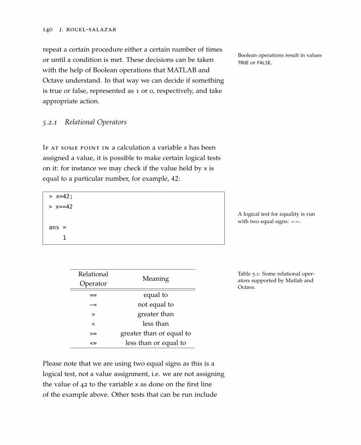
140 j. rogel-salazar

repeat a certain procedure either a certain number of times

or until a condition is met. These decisions can be taken

with the help of Boolean operations that MATLAB and

Boolean operations result in valuesTRUE or FALSE.

Octave understand. In that way we can decide if something

is true or false, represented as 1 or 0, respectively, and take

appropriate action.

5.2.1 Relational Operators

If at some point in a calculation a variable x has been

assigned a value, it is possible to make certain logical tests

on it: for instance we may check if the value held by x is

equal to a particular number, for example, 42:

> x=42;

> x==42

ans =

1

A logical test for equality is runwith two equal signs: ==.

RelationalOperator

Meaning

== equal to~= not equal to> greater than< less than>= greater than or equal to<= less than or equal to

Table 5.1: Some relational oper-ators supported by Matlab andOctave.

Please note that we are using two equal signs as this is a

logical test, not a value assignment, i.e. we are not assigning

the value of 42 to the variable x as done on the first line

of the example above. Other tests that can be run include

essential matlab®

and octave 141

comparisons to see if the value of the variable x is greater

than or less than a given number. Table 5.1 shows some of

the logical operators supported by MATLAB and Octave.

Let us have a look at an example.

Let us consider assigning the value of 2π to the variable x.

we do this with a single equal sign:

> x = 2*pi

x = 6.2832

We can then ask the software to check if x is not equal to 6.

From Table 5.1 we know that the operation “not equal to”

can be carried out with the operator ~=:

> x~=6

ans =

1

The result of the comparison is 1 and thus we know that the

comparison is TRUE, in other words the value held by the

If the result of a comparisonis TRUE the value returned byMATLAB and Octave is 1.

variable x is indeed not equal to 6. Let us see what happens

when we ask if the value held by the variable is not equal to

2π:

> x~=2*pi

ans =

0

In this case the result is FALSE and thus the software re-

turns the value of 0. The comparisons do not necessarily

If the result of a comparisonis FALSE the value returned byMATLAB and Octave is 0.

have to be made with a variable; they can also be made

directly with numbers:

142 j. rogel-salazar

> 42>=24

ans =

1

as well as with the results of calculations:

> pi^2<100

ans =

0

5.2.2 Relational Operators with Vectors and Matrices

As we know, the default type of object handled by

MATLAB and Octave is a matrix, and as such it is natural

to ask how these logical operators are executed on them.

When the object is a vector or a matrix, these tests are done

on an element-by-element basis.

Relational operations can also beused with vectors and matrices.The comparisons are madeelement by element.

For instance, if we consider the matrix:

x =

(0 1 2 3 4

8 2 0 0 0

), (5.1)

and we are interested to know what elements are equal

to zero, we can obtain a Boolean matrix indicating those

elements where the comparison is TRUE with a value of 1

and those where the comparison is FALSE with a value of 0.

The result of a relational operatoron a matrix is a Boolean matrixwhere each element is the result ofthe comparison on an element-by-element basis.Let us enter the matrix shown in Equation (5.1) and make a

comparison with 0:

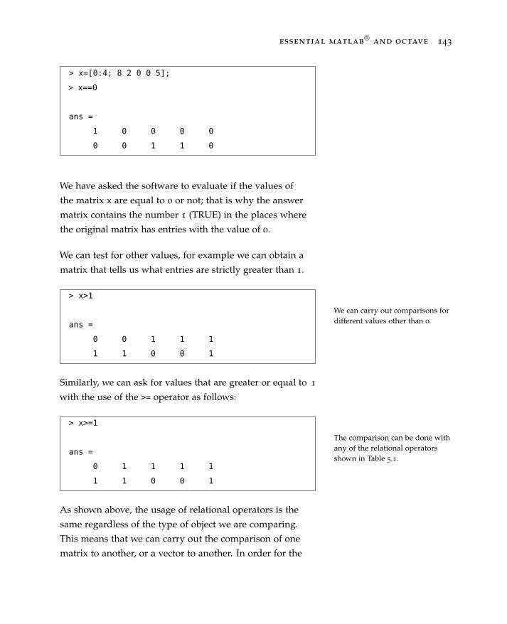
essential matlab®

and octave 143

> x=[0:4; 8 2 0 0 5];

> x==0

ans =

1 0 0 0 0

0 0 1 1 0

We have asked the software to evaluate if the values of

the matrix x are equal to 0 or not; that is why the answer

matrix contains the number 1 (TRUE) in the places where

the original matrix has entries with the value of 0.

We can test for other values, for example we can obtain a

matrix that tells us what entries are strictly greater than 1.

We can carry out comparisons fordifferent values other than 0.

> x>1

ans =

0 0 1 1 1

1 1 0 0 1

Similarly, we can ask for values that are greater or equal to 1

with the use of the >= operator as follows:

The comparison can be done withany of the relational operatorsshown in Table 5.1.

> x>=1

ans =

0 1 1 1 1

1 1 0 0 1

As shown above, the usage of relational operators is the

same regardless of the type of object we are comparing.

This means that we can carry out the comparison of one

matrix to another, or a vector to another. In order for the

144 j. rogel-salazar

comparison to make sense, the only thing we have to take

into account is the fact that the matrices or vectors to be

compared have the same dimensions.

For example, we can compare the following two matrices:

x =

17 24 1 8 15

23 5 7 14 16

4 6 13 20 22

10 12 19 21 3

11 18 25 2 9

, (5.2)

y =

1 2 3 4 5

6 7 8 9 10

11 12 13 14 15

16 17 18 19 20

21 22 23 24 25

, (5.3)

and we are interested to know what elements of x are

greater than those of y.

Comparisons using the relationaloperators from Table 5.1 also workwith matrices and vectors.

We can do this as follows: the first matrix, x, is in fact a 5 × 5

magic matrix:

> x=magic(5)

x =

17 24 1 8 15

23 5 7 14 16

4 6 13 20 22

10 12 19 21 3

11 18 25 2 9

whereas the second one can be constructed with sequences.

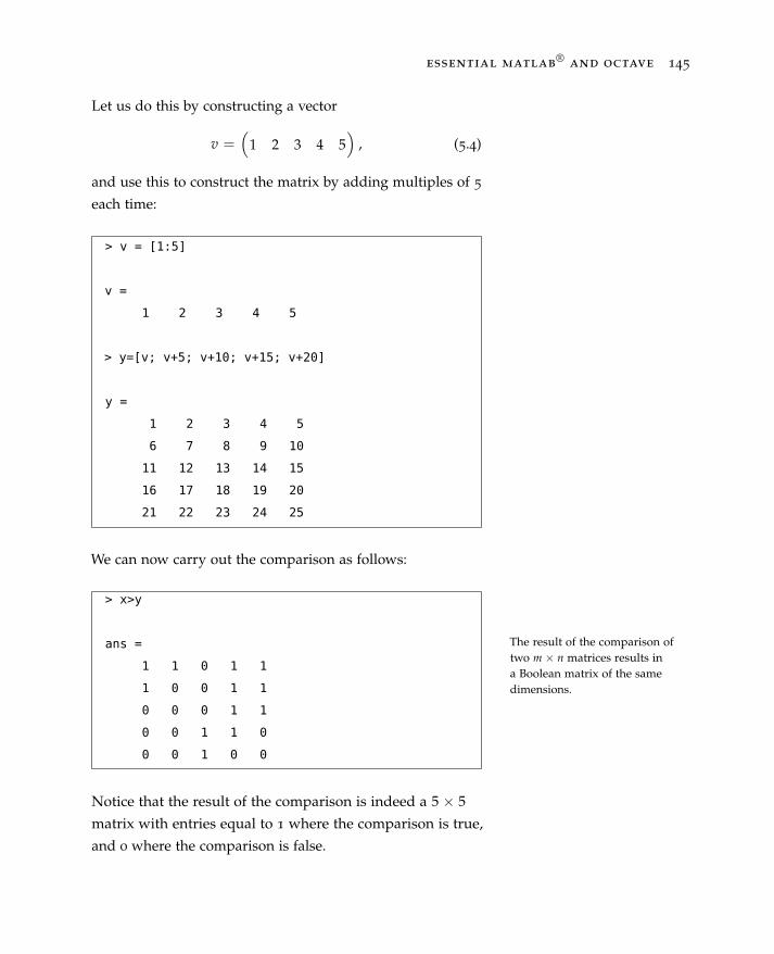
essential matlab®

and octave 145

Let us do this by constructing a vector

v =(

1 2 3 4 5)

, (5.4)

and use this to construct the matrix by adding multiples of 5

each time:

> v = [1:5]

v =

1 2 3 4 5

> y=[v; v+5; v+10; v+15; v+20]

y =

1 2 3 4 5

6 7 8 9 10

11 12 13 14 15

16 17 18 19 20

21 22 23 24 25

We can now carry out the comparison as follows:

> x>y

ans =

1 1 0 1 1

1 0 0 1 1

0 0 0 1 1

0 0 1 1 0

0 0 1 0 0

Notice that the result of the comparison is indeed a 5 × 5

matrix with entries equal to 1 where the comparison is true,

and 0 where the comparison is false.

The result of the comparison oftwo m × n matrices results ina Boolean matrix of the samedimensions.

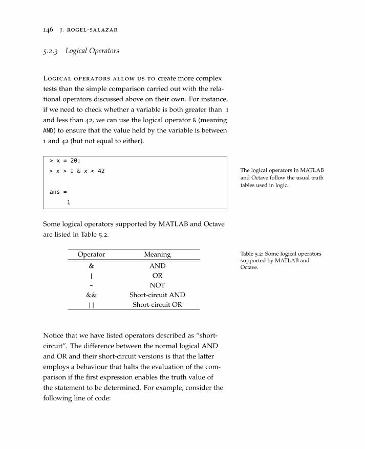
146 j. rogel-salazar

5.2.3 Logical Operators

Logical operators allow us to create more complex

tests than the simple comparison carried out with the rela-

tional operators discussed above on their own. For instance,

if we need to check whether a variable is both greater than 1

and less than 42, we can use the logical operator & (meaning

AND) to ensure that the value held by the variable is between

1 and 42 (but not equal to either).

The logical operators in MATLABand Octave follow the usual truthtables used in logic.

> x = 20;

> x > 1 & x < 42

ans =

1

Some logical operators supported by MATLAB and Octave

are listed in Table 5.2.

Operator Meaning

& AND| OR~ NOT

&& Short-circuit AND|| Short-circuit OR

Table 5.2: Some logical operatorssupported by MATLAB andOctave.

Notice that we have listed operators described as “short-

circuit”. The difference between the normal logical AND

and OR and their short-circuit versions is that the latter

employs a behaviour that halts the evaluation of the com-

parison if the first expression enables the truth value of

the statement to be determined. For example, consider the

following line of code:

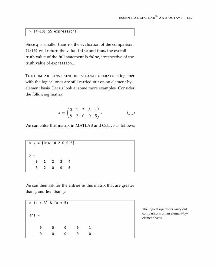
essential matlab®

and octave 147

> (4>10) && expression1

Since 4 is smaller than 10, the evaluation of the comparison

(4>10) will return the value false and thus, the overall

truth value of the full statement is false, irrespective of the

truth value of expression1.

The comparisons using relational operators together

with the logical ones are still carried out on an element-by-

element basis. Let us look at some more examples. Consider

the following matrix:

x =

(0 1 2 3 4

8 2 0 0 5

). (5.5)

We can enter this matrix in MATLAB and Octave as follows:

> x = [0:4; 8 2 0 0 5]

x =

0 1 2 3 4

8 2 0 0 5

We can then ask for the entries in this matrix that are greater

than 3 and less than 5:

The logical operators carry outcomparisons on an element-by-element basis.

> (x > 3) & (x < 5)

ans =

0 0 0 0 1

0 0 0 0 0

148 j. rogel-salazar

The brackets in the expression used in the example above

are not necessary, but they help with reading the combina-

tion of commands entered in the software. We can also ask

for the entries in the matrix shown in Equation (5.5) that are

greater than 3 or equal to 8:

> (x > 3) | (x==8)

ans =

0 0 0 0 1

1 0 0 0 1

Remember that the result of alogical comparison is a Booleanmatrix, where 1 represents thevalue for TRUE and 0 the value forFALSE.

Remember that the logical test for equality is expressed with

the double equal sign as shown in the example above.

5.2.4 Selecting Elements with Logical Operators

Since the logical operators we have discussed are

applied on each element of a vector or matrix, it is possible

to use them in order to select components that do not meet

certain criteria. This is effectively achieved by multiplying,

element-by-element, the original array by a logical one of

the same dimensions.

Let us for example generate a vector with n = 5 elements

drawn from a Gaussian distribution with mean µ = 1 and

standard deviation σ = 2.

The randn(m,n) command generates an m × n matrix

whose elements are uniformly distributed pseudorandom

numbers.

The randn command generatesarrays of uniformly distributedpseudorandom numbers.

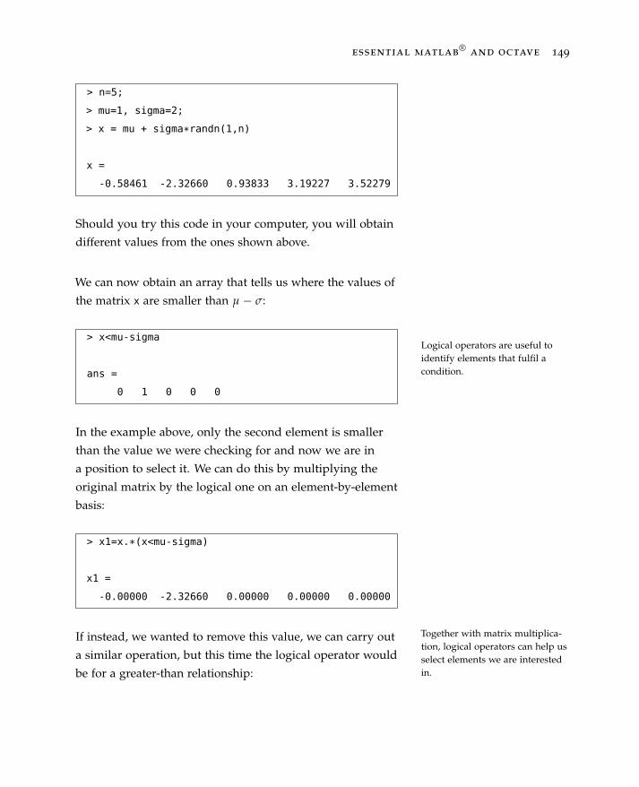
essential matlab®

and octave 149

> n=5;

> mu=1, sigma=2;

> x = mu + sigma*randn(1,n)

x =

-0.58461 -2.32660 0.93833 3.19227 3.52279

Should you try this code in your computer, you will obtain

different values from the ones shown above.

We can now obtain an array that tells us where the values of

the matrix x are smaller than µ − σ:

Logical operators are useful toidentify elements that fulfil acondition.

> x<mu-sigma

ans =

0 1 0 0 0

In the example above, only the second element is smaller

than the value we were checking for and now we are in

a position to select it. We can do this by multiplying the

original matrix by the logical one on an element-by-element

basis:

> x1=x.*(x<mu-sigma)

x1 =

-0.00000 -2.32660 0.00000 0.00000 0.00000

If instead, we wanted to remove this value, we can carry out

a similar operation, but this time the logical operator would

be for a greater-than relationship:

Together with matrix multiplica-tion, logical operators can help usselect elements we are interestedin.

150 j. rogel-salazar

> x2=x.*(x>mu-sigma)

x2 =

-0.58461 -0.00000 0.93833 3.19227 3.52279

In the example outlined above, we have used a small num-

ber of elements and thus it is very easy to determine which

of them are the ones that fulfil the condition tested for.

However, in larger vectors or matrices this may not be so

straightforward. In those cases, it is possible to use the find With larger arrays, the use of thefind command can be a good wayto identify elements that meet acondition.

command in conjunction with logical operators to identify

those elements. For example, let us consider a similar prob-

lem as the one above, except that this time we construct a

5 × 5 matrix with normally distributed elements with the

same parameters as in the previous example:

> n=5;

> mu=1, sigma=2;

In this case we will be using the parameters passed to

the randn command to construct a square matrix with the

desired number of elements:

> x = mu + sigma*randn(n,n)

x =

2.0753 -1.6154 -1.6998 0.5901 2.3430

4.6678 0.1328 7.0698 0.7517 -1.4150

-3.5177 1.6852 2.4508 3.9794 2.4345

2.7243 8.1568 0.8739 3.8181 4.2605

1.6375 6.5389 2.4295 3.8344 1.9778

The find command returns the linear indices of the non- The command find returns thelinear indices of the non-zeroelements of an array.

zero elements of a matrix and thus we can find for example

the elements that are smaller than µ − σ as follows:

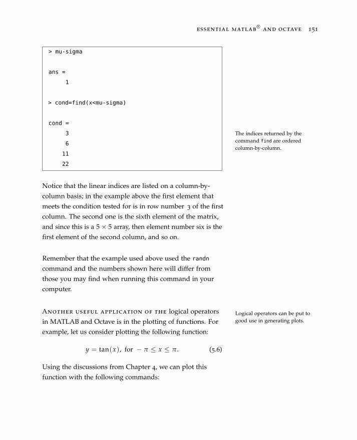
essential matlab®

and octave 151

> mu-sigma

ans =

1

> cond=find(x<mu-sigma)

cond =

3

6

11

22

Notice that the linear indices are listed on a column-by-

column basis; in the example above the first element that

meets the condition tested for is in row number 3 of the first

column. The second one is the sixth element of the matrix,

and since this is a 5 × 5 array, then element number six is the

first element of the second column, and so on.

The indices returned by thecommand find are orderedcolumn-by-column.

Remember that the example used above used the randn

command and the numbers shown here will differ from

those you may find when running this command in your

computer.

Another useful application of the logical operators

in MATLAB and Octave is in the plotting of functions. For

example, let us consider plotting the following function:

Logical operators can be put togood use in generating plots.

y = tan(x), for − π ≤ x ≤ π . (5.6)

Using the discussions from Chapter 4, we can plot this

function with the following commands:

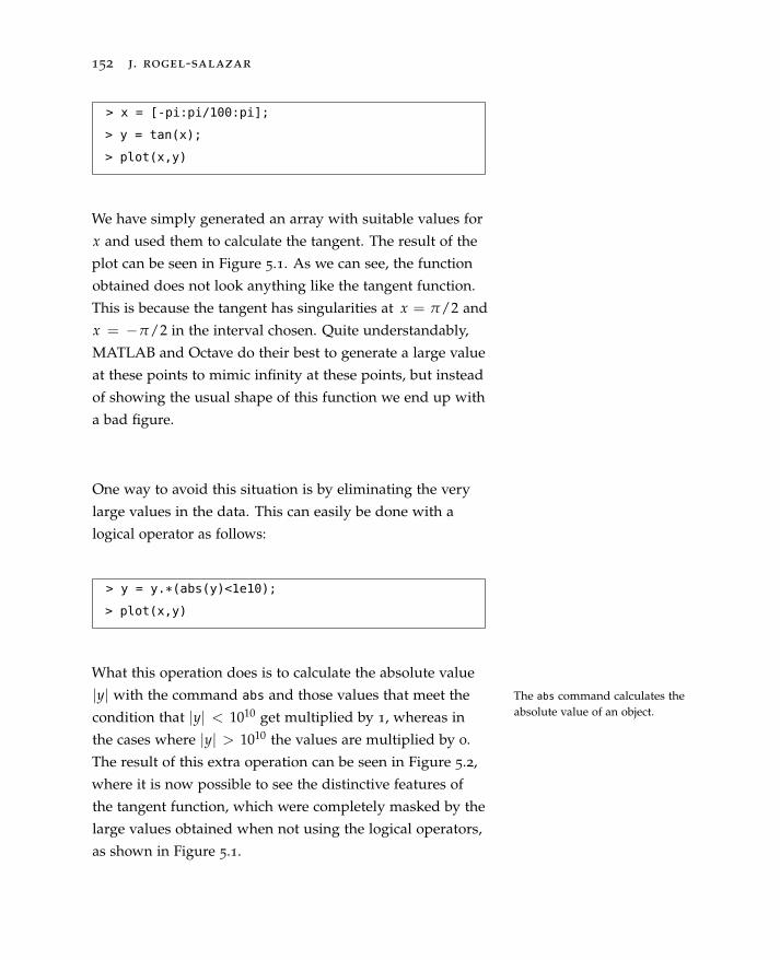
152 j. rogel-salazar

> x = [-pi:pi/100:pi];

> y = tan(x);

> plot(x,y)

We have simply generated an array with suitable values for

x and used them to calculate the tangent. The result of the

plot can be seen in Figure 5.1. As we can see, the function

obtained does not look anything like the tangent function.

This is because the tangent has singularities at x = π/2 and

x = −π/2 in the interval chosen. Quite understandably,

MATLAB and Octave do their best to generate a large value

at these points to mimic infinity at these points, but instead

of showing the usual shape of this function we end up with

a bad figure.

One way to avoid this situation is by eliminating the very

large values in the data. This can easily be done with a

logical operator as follows:

> y = y.*(abs(y)<1e10);

> plot(x,y)

What this operation does is to calculate the absolute value

|y| with the command abs and those values that meet the The abs command calculates theabsolute value of an object.condition that |y| < 1010 get multiplied by 1, whereas in

the cases where |y| > 1010 the values are multiplied by 0.

The result of this extra operation can be seen in Figure 5.2,

where it is now possible to see the distinctive features of

the tangent function, which were completely masked by the

large values obtained when not using the logical operators,

as shown in Figure 5.1.

essential matlab®

and octave 153

ï4 ï3 ï2 ï1 0 1 2 3 4ï4

ï3

ï2

ï1

0

1

2

3

4 x 1015

x

yBad Plot of the Tangent Function

y=tan(x)

Figure 5.1: Plotting functionswith singularities leads to figuresthat do not represent the truecharacteristics of the function. Inthis case we are showing whathappens when trying a naiveapproach when plotting thetangent function y = tan(x).

5.3 Loops in MATLAB and Octave

We mentioned before that it is sometimes desirable to

repeat a certain number of commands depending on values

obtained in the course of the execution of a programme.

Furthermore, in the previous section we have seen how

a comparison between values can be carried out. In this

section we will address how the repetition of steps can be

achieved.

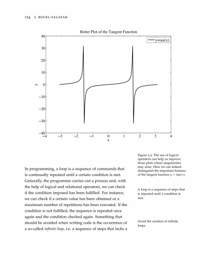
154 j. rogel-salazar

ï4 ï3 ï2 ï1 0 1 2 3 4ï40

ï30

ï20

ï10

0

10

20

30

40

x

yBetter Plot of the Tangent Function

y=tan(x)

Figure 5.2: The use of logicaloperators can help us improvethose plots where singularitiesmay arise. Here we can indeeddistinguish the important featuresof the tangent function y = tan(x).

In programming, a loop is a sequence of commands that

is continually repeated until a certain condition is met.

A loop is a sequence of steps thatis repeated until a condition ismet.

Generally, the programme carries out a process and, with

the help of logical and relational operators, we can check

if the condition imposed has been fulfilled. For instance,

we can check if a certain value has been obtained or a

maximum number of repetitions has been executed. If the

condition is not fulfilled, the sequence is repeated once

again and the condition checked again. Something that

should be avoided when writing code is the occurrence of

a so-called infinite loop, i.e. a sequence of steps that lacks a

Avoid the creation of infiniteloops.

essential matlab®

and octave 155

functioning exit routine. As we shall see below, there are

different kinds of loops.

5.3.1 For Loop

In some procedures it is necessary for the software to

execute a particular instruction a certain predetermined

number of times. This can easily be achieved with a for

loop. The syntax of this type of loop in MATLAB and

Octave is as follows:

For loop: the steps are repeatedfor values of index starting atinitialval and finishing atfinalval. In Octave it is possibleto finish the block with endfor.

for index = initialval:finalval

procedure to be executed for each

value in the loop

end

In the syntax above index is the control variable against

which a logical operation is carried out. The index will first

take the value given by initialval and the loop will stop

when the value finalval is reached; for every value taken

by index the procedure inside the loop will be executed. Let

us have a look at a simple example. Consider the vector

v = (1, 4, 7, 10) , (5.7)

which can be produced with a sequence that starts with

number 1 and finishes with number 10 on steps of value 3:

> v = [1:3:10]

v =

1 4 7 10

Imagine now that we require to change these values with a

linear sequence from 1 to 4. Please note that we can simply

156 j. rogel-salazar

reassign the variable v with the sequence outlined above;

nonetheless this is a simple example to illustrate the use of a

for loop. We can do this as follows:

The for loop syntax requires theuse of end to terminate the loop.

> for j=1:4, v(j)=j; end

> v

v =

1 2 3 4

In this example we have started with the vector given by

Equation (5.7) and used a for loop to reassign its elements

to the values of the index j going from 1 to 4. This is a

simple demonstration of how this loop works, but it is not

very practical given the procedural nature of the software,

as looping through a vector in this way is very slow. Instead

we could have used a syntax similar to the first statement

in the example above and which is more natural in both

MATLAB and Octave.

In the example above the for loop moved in steps of 1 from

the initial value to the end value; we can also require that

the sequence moves with different step values. In this case,

the syntax of the loop makes use of the colon notation we

are familiar with:

for index = initialval:step:finalval

procedure to be executed for each

value in the loop

end

We can use the colon notation tochange the step in the for loop.

The loop will start at the value given by initialval and

every iteration will be executed until the value finalval is

reached; this will be done by changing the index on every

iteration by the value given by step.

essential matlab®

and octave 157

For example, let us consider the case where we want to

generate the following vector with a for loop:

v = (1, 3, 5, 7) . (5.8)

We can do this as follows: let us start a counter variable

k that controls the elements of the array and as such we

initialise it with the value of 1. We can then set up a for

loop starting at 1 and finishing at 8, changing the index j

with a step equal to 2. Before each iteration is completed we

add one to the control variable k so that the next value is

stored in the correct place:

The use of a control variable thatis changed within the loop givesus the flexibility we may require inconstructing loops.

> k=1;

> for j=1:2:8 ...

v(k)=j;...

k=k+1;...

end;

We can easily check that the values stored in the vector v are

as expected:

> v

v =

1 3 5 7

The for loop used to constructthis vector is not very practical.Vectorisation should instead beused.

Before we move on, let us mention a couple of points. It

is usually the case that programmers use the variables i,

j or k to denote the controls in a loop. This is indeed true Remember that i and j are alsoused to represent the complexnumber i.

in the case of MATLAB and Octave, too. Nonetheless, we

urge some caution as the i and j are used in the software to

denote the complex number i.

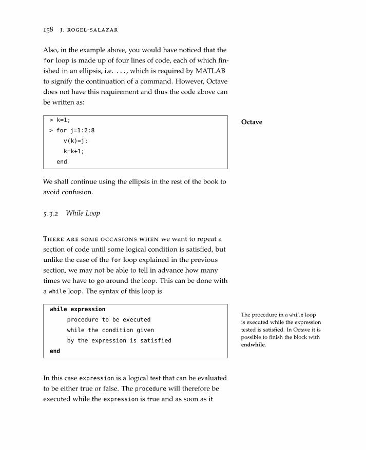
158 j. rogel-salazar

Also, in the example above, you would have noticed that the

for loop is made up of four lines of code, each of which fin-

ished in an ellipsis, i.e. ..., which is required by MATLAB

to signify the continuation of a command. However, Octave

does not have this requirement and thus the code above can

be written as:

Octave> k=1;

> for j=1:2:8

v(k)=j;

k=k+1;

end

We shall continue using the ellipsis in the rest of the book to

avoid confusion.

5.3.2 While Loop

There are some occasions when we want to repeat a

section of code until some logical condition is satisfied, but

unlike the case of the for loop explained in the previous

section, we may not be able to tell in advance how many

times we have to go around the loop. This can be done with

a while loop. The syntax of this loop is

The procedure in a while loopis executed while the expressiontested is satisfied. In Octave it ispossible to finish the block withendwhile.

while expression

procedure to be executed

while the condition given

by the expression is satisfied

end

In this case expression is a logical test that can be evaluated

to be either true or false. The procedure will therefore be

executed while the expression is true and as soon as it

essential matlab®

and octave 159

is false, the loop will stop. For example, starting with the

value of 0, we would like to print a sequence of numbers

less than 3. This can be done with the following code:

> n=0;

> while n<3 ...

n = n+1 ...

end

n =

1

n =

2

n =

3

The while loop tests the conditionbefore each iteration is carried out.

Notice that we need to change the value of the control

variable n inside the while loop; this helps us avoid the

creation of an infinite loop as eventually the condition is no

longer satisfied. Note also that the logical test is carried out

at the beginning of the loop. This is important as the loop

may not even execute once if the condition is not met. For

example, consider the following code:

If the condition is not met at thebeginning of the while iteration,the code inside the loop is notexecuted.

> n=10;

> while n<3 ...

n = n+1 ...

end

Since the initial value of the control variable n is 10, the first

time the condition is tested results in a FALSE value and the

loop is not executed.

160 j. rogel-salazar

It can be very helpful to use a while loop in program-

ming flows that require that a certain condition is met

before the next iteration takes place. Let us look at an exam-

ple. Consider solving the following equation numerically:

x = cos2(x). (5.9)

We can start with a guess of say π/2 and then compute

a sequence of values for xn = cos2(xn−1), where n is

the number of iterations, and continue until the difference

between consecutive values xn and xn−1 is smaller than

a tolerance given. We can start by defining some useful

parameters in the solution of Equation (5.9):

> x_guess = pi/2;

> n=1;

> difference=1;

where x_guess is our initial guess, n assigns the value for

the first iteration and we define an initial difference for

comparison purposes. We can now set up a while loop:

The while loop can be very usefulto test that a certain condition ismet before the next iteration takesplace.

> while (difference > 0.001) && (n< 200) ...

n = n+1; ...

x_new=cos(x_guess)^2; ...

difference = abs(x_new - x_guess); ...

x_guess = x_new; ...

end

> n

n =

146

> x_guess

x_guess =

0.6412

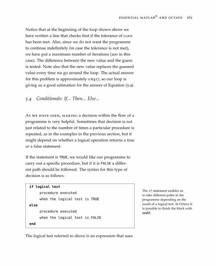
essential matlab®

and octave 161

Notice that at the beginning of the loop shown above we

have written a line that checks first if the tolerance of 0.001

has been met. Also, since we do not want the programme

to continue indefinitely (in case the tolerance is not met),

we have put a maximum number of iterations (200 in this

case). The difference between the new value and the guess

is tested. Note also that the new value replaces the guessed

value every time we go around the loop. The actual answer

for this problem is approximately 0.6417, so our loop is

giving us a good estimation for the answer of Equation (5.9).

5.4 Conditionals: If... Then... Else...

As we have seen, making a decision within the flow of a

programme is very helpful. Sometimes that decision is not

just related to the number of times a particular procedure is

repeated, as in the examples in the previous section, but it

might depend on whether a logical operation returns a true

or a false statement.

If the statement is TRUE, we would like our programme to

carry out a specific procedure, but if it is FALSE a differ-

ent path should be followed. The syntax for this type of

decision is as follows:

The if statement enables usto take different paths in theprogramme depending on theresult of a logical test. In Octave itis possible to finish the block withendif.

if logical test

procedure executed

when the logical test is TRUE

else

procedure executed

when the logical test is FALSE

end

The logical test referred to above is an expression that uses

162 j. rogel-salazar

the relational and logical operators defined in Sections 5.2.1

and 5.2.3, respectively.

Let us have a look at a simple example. Given the expres-

sions cos(π/3) and sin(π/3) we want to write some code

that tests which one is larger and display a message accord-

ingly. We can use the if... then... else statement as

follows:

We are using the disp commandto print a message to the terminal.

> a = cos(pi/3); b = sin(pi/3);

> if a > b ...

disp(’cos(pi/3) is bigger than sin(pi/3)’)...

else ...

disp(’sin(pi/3) is bigger than cos(pi/3)’)...

end

sin(pi/3) is bigger than cos(pi/3)

In the example above we have used the command disp to

display a message to the terminal. In this case, since

sin(π

3

)=

√3

2' 0.8660 (5.10)

is a bigger value than

cos(π

3

)=

12= 0.5, (5.11)

then the logical test is not TRUE and therefore only the

statement after else is displayed.

In other cases there may be more than one path that the

programme should follow, depending on whether a set of

conditions is either TRUE or FALSE. In those cases a nested

if... then... else... can be used; however, there is a

shortcut offered by MATLAB and Octave:

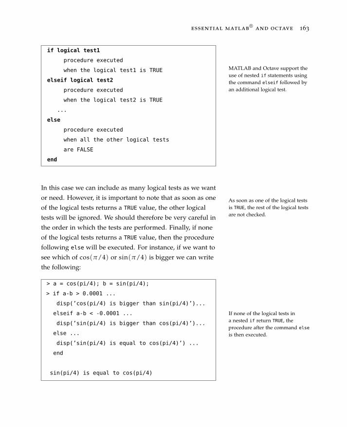
essential matlab®

and octave 163

if logical test1

procedure executed

when the logical test1 is TRUE

elseif logical test2

procedure executed

when the logical test2 is TRUE

...

else

procedure executed

when all the other logical tests

are FALSE

end

MATLAB and Octave support theuse of nested if statements usingthe command elseif followed byan additional logical test.

In this case we can include as many logical tests as we want

or need. However, it is important to note that as soon as one

of the logical tests returns a TRUE value, the other logical

tests will be ignored. We should therefore be very careful in

the order in which the tests are performed. Finally, if none

As soon as one of the logical testsis TRUE, the rest of the logical testsare not checked.

of the logical tests returns a TRUE value, then the procedure

following else will be executed. For instance, if we want to

see which of cos(π/4) or sin(π/4) is bigger we can write

the following:

If none of the logical tests ina nested if return TRUE, theprocedure after the command else

is then executed.

> a = cos(pi/4); b = sin(pi/4);

> if a-b > 0.0001 ...

disp(’cos(pi/4) is bigger than sin(pi/4)’)...

elseif a-b < -0.0001 ...

disp(’sin(pi/4) is bigger than cos(pi/4)’)...

else ...

disp(’sin(pi/4) is equal to cos(pi/4)’) ...

end

sin(pi/4) is equal to cos(pi/4)

164 j. rogel-salazar

We have written the code in this way, i.e. providing a toler-

ance for the comparison, in order to avoid the fact that there

are rounding errors when computing the values required.

Since neither the first not the second logical tests were TRUE,

the code displays the message after the else statement.

5.5 Procedures and Functions with m-Files

As mentioned earlier on, up until now we have been

using MATLAB and Octave effectively as sophisticated

line-by-line calculators. However, they can be used in a

much more powerful way by writing scripts. This allows

us to create more complicated programmes and automate

a number of tasks as well as repeat calculations by running

the script, instead of typing commands again and again.

An m-file is a simple text file thatenlists a series of commands tobe executed. If the script acceptsinputs and returns outputs thenwe call it a function.

We know that these scripts are referred to as m-files. When

an m-file is run, the commands written in the script are

interpreted one by one as explained in Section 5.1.

When these m-files are used for executing specific tasks

given an input and the result is an expected output, then we

refer to function m-files.

5.5.1 Putting It All Together: m-Files

If we want to execute repeatedly a given set of com-

mands, we can create an m-file that lists these commands

and stores them for later use. For example, let us consider a

situation where we want to be able to plot a sine or cosine

function with a given frequency between −π and π.

We can indeed use the terminal as we have done so far, but

as soon as we want to change the frequency of the function,

essential matlab®

and octave 165

for instance, then we have to re-type all the different com-

mands. However, we can create a script that can be saved in

our computer and later retrieved. All we would have to do

then is to test whether we want to plot the sine or the cosine,

modify the frequency of the trigonometric function to be

plotted, run the script and we are done.

One important thing to remember is that unlike in the

examples we have seen in the previous sections, the scripts

do not need to end each line in the code with an ellipsis,

unless we truly are splitting a single long command.

m-files do not need the use of anellipsis (...) at the end of eachline.

Let us tackle the creation of the m-file that can be used for

the task of plotting either the sine or cosine functions as

mentioned above. First we will create a text file that will

hold the commands and instructions so that they are readily

available at a later stage. It is important to mention that in

order for MATLAB and Octave to execute the script, you

must be in the folder or directory where the file is saved.

In this case we will name our script my_plot_script.m.

Remember that you can use your favourite text editor as

explained in Section 5.1.1.

It usually helps to have a brief plan of the tasks we need to

accomplish to tackle our problem. For instance, in this case

we can take into account the following list:

1. Make sure that the workspace is clear.

2. Define a variable to hold the frequency of the trigonomet-

ric function.

3. Define the range of values to plot the trigonometric

function.

4. Decide if the sine or the cosine will be plotted.

5. Create the plot and format it.

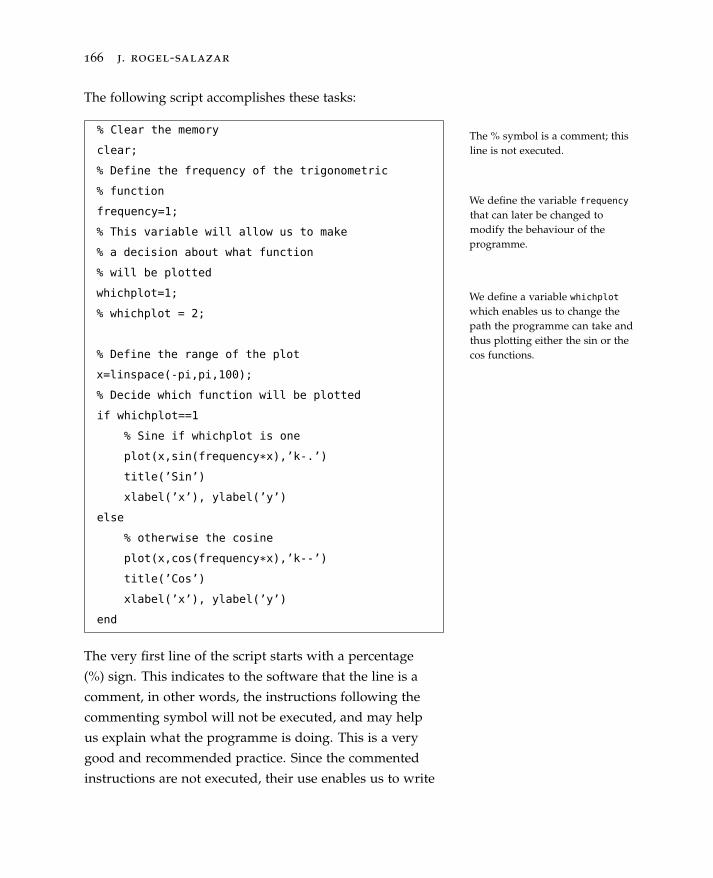
166 j. rogel-salazar

The following script accomplishes these tasks:

The % symbol is a comment; thisline is not executed.

We define the variable frequency

that can later be changed tomodify the behaviour of theprogramme.

We define a variable whichplot

which enables us to change thepath the programme can take andthus plotting either the sin or thecos functions.

% Clear the memory

clear;

% Define the frequency of the trigonometric

% function

frequency=1;

% This variable will allow us to make

% a decision about what function

% will be plotted

whichplot=1;

% whichplot = 2;

% Define the range of the plot

x=linspace(-pi,pi,100);

% Decide which function will be plotted

if whichplot==1

% Sine if whichplot is one

plot(x,sin(frequency*x),’k-.’)

title(’Sin’)

xlabel(’x’), ylabel(’y’)

else

% otherwise the cosine

plot(x,cos(frequency*x),’k--’)

title(’Cos’)

xlabel(’x’), ylabel(’y’)

end

The very first line of the script starts with a percentage

(%) sign. This indicates to the software that the line is a

comment, in other words, the instructions following the

commenting symbol will not be executed, and may help

us explain what the programme is doing. This is a very

good and recommended practice. Since the commented

instructions are not executed, their use enables us to write

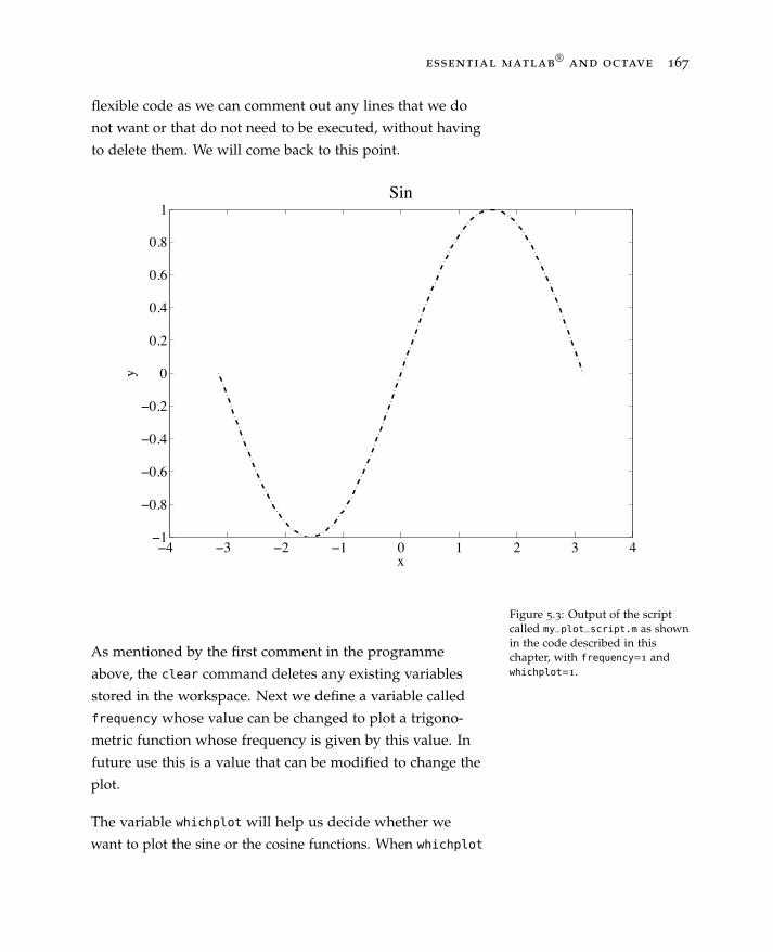
essential matlab®

and octave 167

flexible code as we can comment out any lines that we do

not want or that do not need to be executed, without having

to delete them. We will come back to this point.

ï4 ï3 ï2 ï1 0 1 2 3 4ï1

ï0.8

ï0.6

ï0.4

ï0.2

0

0.2

0.4

0.6

0.8

1Sin

x

y

Figure 5.3: Output of the scriptcalled my_plot_script.m as shownin the code described in thischapter, with frequency=1 andwhichplot=1.

As mentioned by the first comment in the programme

above, the clear command deletes any existing variables

stored in the workspace. Next we define a variable called

frequency whose value can be changed to plot a trigono-

metric function whose frequency is given by this value. In

future use this is a value that can be modified to change the

plot.

The variable whichplot will help us decide whether we

want to plot the sine or the cosine functions. When whichplot

168 j. rogel-salazar

equals one, we will plot the sine; otherwise we plot the co-

sine. Please notice that we have commented out a line

where whichplot is given a value different from one; and

remember that this line will not be executed.

Since a commented line is notexecuted, we can use this to re-uselines of code at a later stage.

The decision regarding what plot is shown is made with

an if statement. When the variable whichplot is equal to

1 we plot the sine function in black with a dash-dot pat-

tern; otherwise we plot the cosine function in black with a

dashed line pattern. With the programme written as shown

above, we would obtain a plot of the sine function sin(x)and the result is shown in Figure 5.3. If instead we wanted

to plot cos(3x) we need to change the value of the variable

frequency from 1 to 3 and the variable whichplot to 2, or

uncomment the appropriate line, and run the programme

again. The result of these changes can be seen in Figure 5.4. The scripting capabilities ofMATLAB and Octave are anessential feature of the languageand offer great flexibility to us asprogrammers.

All we had to do to create these figures was to change a

couple of values and re-run the programme; compare this

with the prospect of having to re-write the entire series of

commands just to change the frequency of the function. As

you can imagine, when the number of lines of code becomes

larger and larger, the flexibility offered by the scripting capa-

bilities of MATLAB and Octave becomes an essential feature

of the language.

5.5.2 Functions in m-Files

In the previous section we have seen how to put

commands together in a script. However, it is sometimes

useful to write programmes that take an input, carry out a

prescribed procedure and return an output.

These scripts are known as function m-files and they also

have the “.m” extension. Let us consider a function m-file

A function m-file is a script thattakes an input, executes someoperations and returns an output.

essential matlab®

and octave 169

ï4 ï3 ï2 ï1 0 1 2 3 4ï1

ï0.8

ï0.6

ï0.4

ï0.2

0

0.2

0.4

0.6

0.8

1Cos

x

y

Figure 5.4: Output of the scriptcalled my_plot_script.m. forfrequency=3 and whichplot=2.called myfunction.m. The structure of the function m-file is

the following:

function [out1,out2,...]=myfunction(in1,in2, ...)

% Comments to be used as help for the function

% Shown when requesting help about the function

Code to be executed when

this function is called

out1= ...

out2= ...

end

170 j. rogel-salazar

There are several things to note here:

• First of all, the script starts with the word function. The script starts with the keywordfunction.

• We then have the variables where the outputs of the

procedure will be returned (in square brackets), in this

case out1, out2, etc.

The output variables are placed insquare brackets.

• Note that the next character is an equal sign followed by

the name of the function. It is important to note that the

name of the function must correspond to the name of the

script. In this case, since the function is called myfunction

the script must be saved with the name myfunction.m.

The name of the function and thename of the file must be the same.

• The name of the function is followed by the variables that

are used to store the inputs (in round brackets).The input variables are placed inround brackets.

• We must assign the values that the function is expected to

return.The output variables must beassigned a return value.

• Finally, it is important to realise that the input and output

variables in1, in2,... out1, out2,... are dummyvariables. In other words, they serve as placeholders

within the definition of the function and their scope is

valid only inside the function itself.

The input and output argumentsare dummy variables.

The fact that the input and output arguments are dummy

variables provides flexibility when writing code as well as at

running time. This means that we do not necessarily have to

use the variable names used in the definition when calling

the function with actual input arguments.

Let us have a look at an example. Imagine that we need

to calculate the area and circumference of a circle of a

given diameter d. We can do this directly in the terminal.

However, we can write a function that can be re-used to

calculate these measures for any given circle.

essential matlab®

and octave 171

function [area, circumference] = my_circle(d)

% This function calculates the area and

% circumference of a circle of diameter d.

% Let us calculate the radius

r = d/2;

% We can use r to calculate the area

area= pi*r^2;

% and the circumference

circumference = 2*pi*r;

end

A function that takes a diameter das an input, and returns the area

and circumference of a circle.

We shall save the function in a file called my_circle.m. We

can then call the function from the command line in the

software, for instance for a circle of diameter 3.

We can call the function as it isdone for any other MATLAB andOctave command.

> [a,c]=my_circle(3)

a =

7.0686

c =

9.4248

In this case, the first variable will receive the result for the

area, whereas the second one the result for the circumfer-

ence.

You will notice that after the definition of the function, we

have included a couple of comments. These comments

are usually used to provide an explanation about what

the function does and how to use it. Not only is this help

172 j. rogel-salazar

available when looking at the function file, but it is also

available in the command line. We can obtain the help

provided by the comments at the beginning of the function

by using the help command followed by the name of the

function:

The help command can be used todisplay the explanation added tothe function file.

> help my_circle

This function calculates the area and

circumference of a circle of diameter d.

Finally, a word of caution: MATLAB and Octave have a

number of built-in functions (see Section 5.6), and you

should avoid re-using the same name of any of those ex-

isting functions when writing your own. If for whatever

reason you end up naming a function with the name of an

existing one, remember that MATLAB and Octave apply

precedence rules summarised as follows:

1. Before running a function, MATLAB and Octave check if

there are any existing variables in the current workspace

that match the name given. If so, you cannot run the

function until the variable is cleared from the workspace.

Precedence for the usage offunctions.

2. Local functions within the current file take precedence.

3. If no local function is present, MATLAB and Octave check

for functions in the current folder.

4. Finally, functions elsewhere on the path are used, in

order of appearance.

5.6 Built-In Functions

MATLAB and Octave include a number of ready-madeMATLAB and Octave have anumber of functions that areready to be used.

m-files that perform a number of procedures and as such

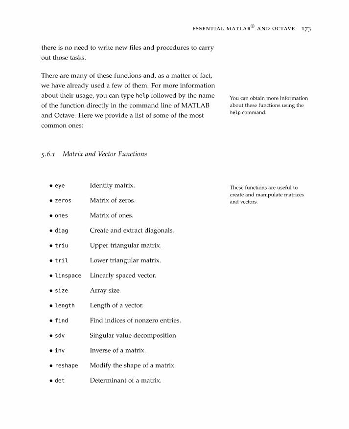
essential matlab®

and octave 173

there is no need to write new files and procedures to carry

out those tasks.

There are many of these functions and, as a matter of fact,

we have already used a few of them. For more information

about their usage, you can type help followed by the name

of the function directly in the command line of MATLAB

and Octave. Here we provide a list of some of the most

common ones:

You can obtain more informationabout these functions using thehelp command.

5.6.1 Matrix and Vector Functions

These functions are useful tocreate and manipulate matricesand vectors.

• eye Identity matrix.

• zeros Matrix of zeros.

• ones Matrix of ones.

• diag Create and extract diagonals.

• triu Upper triangular matrix.

• tril Lower triangular matrix.

• linspace Linearly spaced vector.

• size Array size.

• length Length of a vector.

• find Find indices of nonzero entries.

• sdv Singular value decomposition.

• inv Inverse of a matrix.

• reshape Modify the shape of a matrix.

• det Determinant of a matrix.

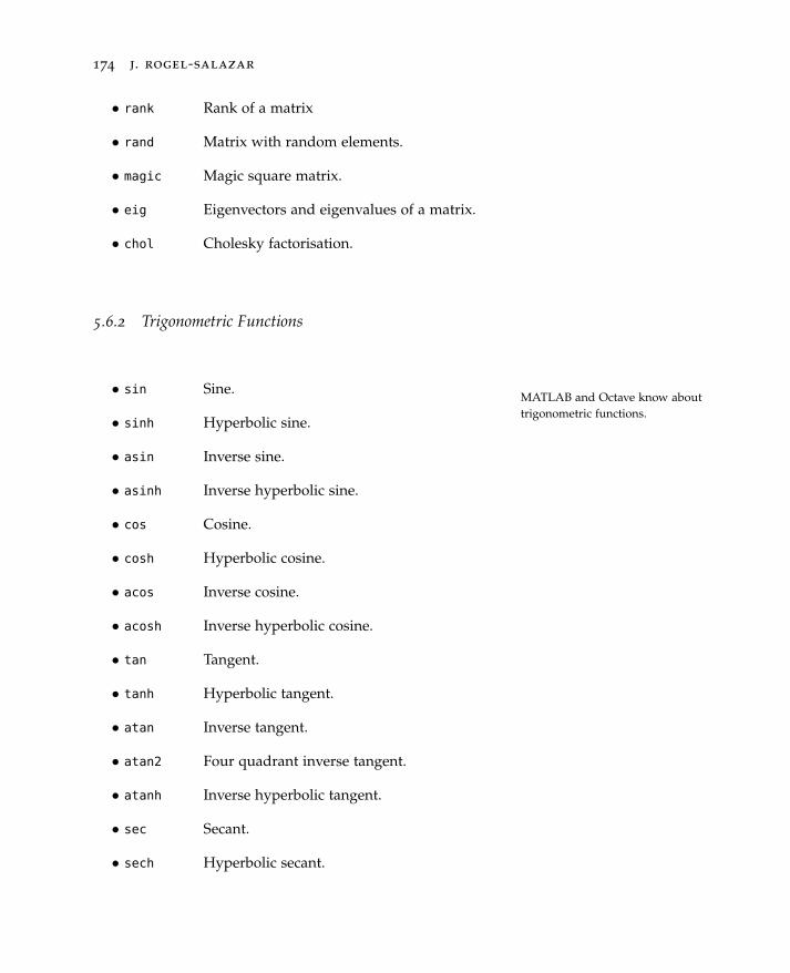
174 j. rogel-salazar

• rank Rank of a matrix

• rand Matrix with random elements.

• magic Magic square matrix.

• eig Eigenvectors and eigenvalues of a matrix.

• chol Cholesky factorisation.

5.6.2 Trigonometric Functions

MATLAB and Octave know abouttrigonometric functions.

• sin Sine.

• sinh Hyperbolic sine.

• asin Inverse sine.

• asinh Inverse hyperbolic sine.

• cos Cosine.

• cosh Hyperbolic cosine.

• acos Inverse cosine.

• acosh Inverse hyperbolic cosine.

• tan Tangent.

• tanh Hyperbolic tangent.

• atan Inverse tangent.

• atan2 Four quadrant inverse tangent.

• atanh Inverse hyperbolic tangent.

• sec Secant.

• sech Hyperbolic secant.

essential matlab®

and octave 175

• asec Inverse secant.

• asech Inverse hyperbolic secant.

• csc Cosecant.

• csch Hyperbolic cosecant.

• acsc Inverse cosecant.

• acsch Inverse hyperbolic cosecant.

• cot Cotangent.

• coth Hyperbolic cotangent.

• acot Inverse cotangent.

• acoth Inverse hyperbolic cotangent.

5.6.3 Functions for Complex Numbers

These functions enable us tomanipulate complex numbers andfunctions.

• abs Absolute value.

• angle Phase angle.

• conj Complex conjugate.

• imag Complex imaginary part.

• real Complex real part.

• unwrap Unwrap phase angle.

• isreal True for real array.

• cplxpair Sort numbers into complex conjugate pairs

176 j. rogel-salazar

5.6.4 Exponential and Logarithmic Functions

These functions let us use expo-nentials and logarithms.

• exp Exponential.

• log Natural logarithm.

• log10 Common (base 10) logarithm.

• log2 Base 2 logarithm and dissect floating point

number.

• pow2 Base 2 power and scale floating point

number.

• sqrt Square root.

• nextpow2 Next higher power of 2.

5.6.5 Rounding and Reminder Functions

The functions listed here providesupport for rounding numbersand calculating reminders.

• fix Round towards zero.

• floor Round towards minus infinity.

• ceil Round towards plus infinity.

• round Round towards nearest integer.

• mod Modulus (signed remainder after division).

• rem Remainder after division.

• sign Signum.

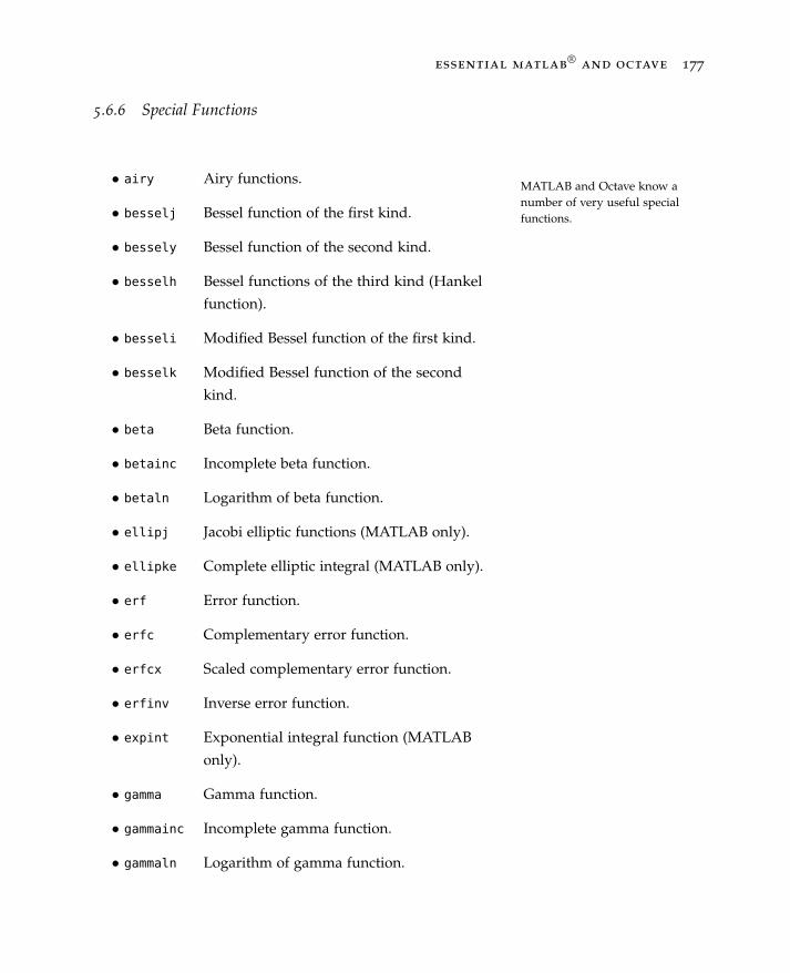
essential matlab®

and octave 177

5.6.6 Special Functions

MATLAB and Octave know anumber of very useful specialfunctions.

• airy Airy functions.

• besselj Bessel function of the first kind.

• bessely Bessel function of the second kind.

• besselh Bessel functions of the third kind (Hankel

function).

• besseli Modified Bessel function of the first kind.

• besselk Modified Bessel function of the second

kind.

• beta Beta function.

• betainc Incomplete beta function.

• betaln Logarithm of beta function.

• ellipj Jacobi elliptic functions (MATLAB only).

• ellipke Complete elliptic integral (MATLAB only).

• erf Error function.

• erfc Complementary error function.

• erfcx Scaled complementary error function.

• erfinv Inverse error function.

• expint Exponential integral function (MATLAB

only).

• gamma Gamma function.

• gammainc Incomplete gamma function.

• gammaln Logarithm of gamma function.

178 j. rogel-salazar

• legendre Associated Legendre function.

• cross Vector cross product.

5.6.7 Number Theoretic Functions

MATLAB and Octave providesupport for number theory.

• factor Prime factors.

• isprime True for prime numbers.

• primes Generate list of prime numbers.

• gcd Greatest common divisor.

• lcm Least common multiple.

• rat Rational approximation.

• rats Rational output.

• perms All possible permutations.

• nchoosek All combinations of n elements taken k at a

time.

5.6.8 Coordinate Transformations

It is possible to carry out basiccoordinate transformations withMATLAB and Octave.

• cart2sph Transform Cartesian to spherical coordi-

nates.

• cart2pol Transform Cartesian to polar coordinates.

• pol2cart Transform polar to Cartesian coordinates.

• sph2cart Transform spherical to Cartesian coordi-

nates.

essential matlab®

and octave 179

• hsv2rgb Convert hue-saturation-value colours to

red-green-blue (MATLAB only).

• rgb2hsv Convert red-green-blue colours to hue-

saturation-value (MATLAB only).

5.6.9 Statistics

Some statistics functions availablein MATLAB and Octave.

• mean Arithmetic mean.

• median Median.

• cov Variance and covariance.

• corrcoef Correlation.

• sum Sum of elements.

• prod Product of elements.

• hist Histogram.

• max Largest element.

• min Smallest element.

5.6.10 Data Interpolation

Functions to deal with data inter-polation and spline interpolation.

• pchip Piecewise cubic Hermite interpolation.

• interp1 1D interpolation.

• interp1q 1D interpolation without error checking.

• interp2 2D interpolation.

180 j. rogel-salazar

• interp2 3D interpolation.

• interpn N-dimensional interpolation.

• griddata Regular mesh from irregular data using

interpolation.

• spline Cubic spline interpolation.

5.6.11 Polynomials

Functions to deal with polynomi-als and fitting.

• roots Find the roots of a polynomial.

• poly Convert roots to a polynomial.

• polyval Polynomial evaluation.

• polyvalm Polynomial evaluation with a matrix argu-

ment.

• residue Partial fraction expansion.

• polyfit Fit polynomial to data.

• polyder Polynomial differentiation.

• polyint Polynomial integration.

• conv Convolution.

• deconv Deconvolution.

essential matlab®

and octave 181

5.6.12 Finite Differences

MATLAB and Octave know howto calculate finite differences.

• diff Approximate derivative.

• gradient Approximate gradient.

• del2 Discrete Laplacian.

5.6.13 Differential Equations

MATLAB and Octave have manyother functions to deal with ODEs;please check the help.

• ode45 Runge-Kutta Method (only MATLAB).

• lsode Ordinary differential equation solver (only

Octave).

5.6.14 Optimisation and Root Finding

Optimisation and root findingfunctions.

• fminbnd Scalar bounded nonlinear function minimi-

sation.

• fzero Scalar nonlinear zero finding.

5.6.15 Fourier Transforms

Functions to deal with Fouriertransforms.

• fft Fast Fourier transform.

• fft2 2D fast Fourier transform.

• fftn N-dimensional fast Fourier transform.

182 j. rogel-salazar

• ifft Inverse fast Fourier transform.

• ifft2 Inverse 2D fast Fourier transform.

• ifftn Inverse N-dimensional fast Fourier trans-

form.

• fftshift Shift zero-frequency to the centre of spec-

trum.

• ifftshift Inverse fftshift.

5.7 Function Handles

In this chapter we have seen how to construct and

programme a function in MATLAB and Octave. Although

these functions can be used with good effect to build more

complex programmes, sometimes it is necessary to exploit

further capabilities offered by the software.

For example, from time to time when a process requires that

a function calls another function, it may be more straight-

forward to call the second function indirectly. In order to

do that we need to use a function handle, which allows us to A function handle lets us manip-ulate a function from anotherfunction.

do various things such as calling a function from another

function, creating functions of functions, and even storing

them in data structures that can be recalled later.

In order to build a function handle we simply need to put

the @ symbol before the name of the function; for instance if

we have a function called MyFunctionName, a handle fhandle

for this function is defined as follows:

A function handle is denoted bythe use of the @ symbol.

fhandle = @ MyFunctionName

The software will map the handle to the specified function

and this information is stored in the handle itself. It is

essential matlab®

and octave 183

important to note that a handle will keep this mapping even

when the function is out of scope. For example, if during

the execution of a programme the path is changed and

another function with the same name has a higher priority,

the handle will still call the original function stored in the

older path. Please refer to the last part of Section 5.5.2 for a

brief discussion of function precedence.

A function handle has a persis-tent mapping to the function itrefers to, regardless of functionprecedence rules.

In the following sections we will discuss some applications

of function handles.

5.7.1 Anonymous Functions

Handles can be used very effectively when we need to

define a function on the fly, in other words, a procedure that

is simple enough to be defined in a programme without the

need of creating a separate m-file. These type of functions

are called anonymous functions. The syntax of an anonymous

function is as follows:

An anonymous function is simpleenough to be defined in one lineof code.

function_name = @(var) expression with var

where var is the variable used in the function.

For example, if we wanted to calculate repeatedly the value

of the following expression:

f (x) = x3 + 3x − 1, (5.12)

we would like to do this for various values of x, and thus

we can certainly write the full expression every time, or

create a function in a separate m-file. However, this can be

simplified greatly with an anonymous function defined as

follows:

An anonymous function can beused for simple processes that donot require a full m-file of theirown.

184 j. rogel-salazar

> CUBIC = @(x) x.^3+3*x-1;

We have defined a function called CUBIC where the input

is given by the variable x. We know this because x is the

variable enclosed in the expression @(). This is followed by

the expression given in Equation (5.12). All we have to do to

use this function is simply call it as we have been doing for

other functions:

An anonymous function can beexecuted in the same way otherfunctions are.

> CUBIC(1)

ans =

3

> CUBIC(2)

ans =

13

5.7.2 Arrays of Function Handles

As we mentioned before, it is possible to store func-

tion handles as we do any other variable. We can think of

function handles as objects that point to other functions and

facilitate their use without using complicated manipulations.

Let us take a look at the following example. We can create

a function handle for any built-in function; for instance

we can do so for the sine or any of the other trigonometric

functions:

> sine_handle = @sin;

As such, we can use the new handle as a synonym for the

function:

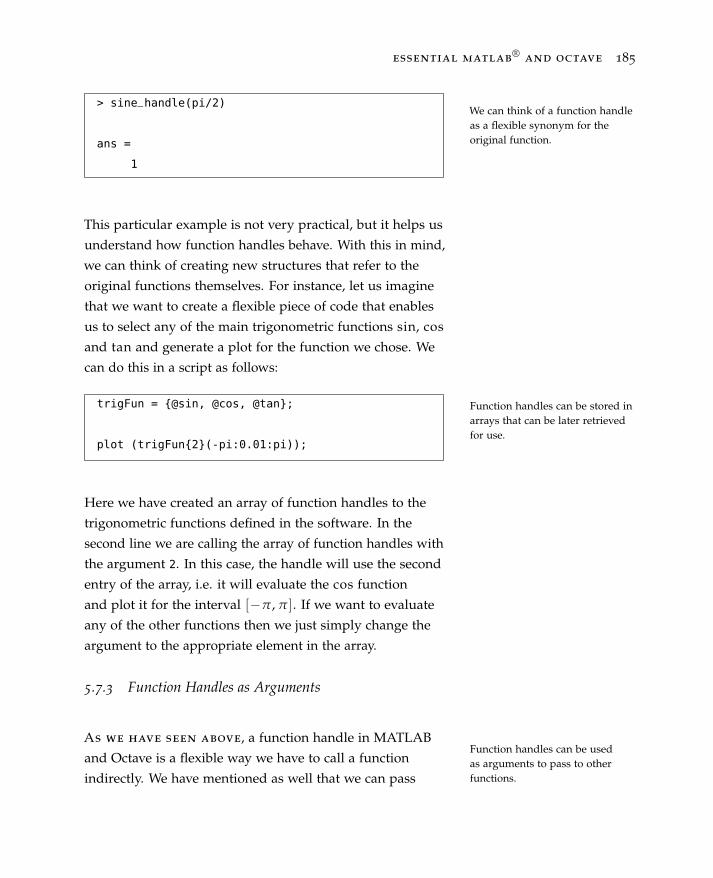
essential matlab®

and octave 185

> sine_handle(pi/2)

ans =

1

We can think of a function handleas a flexible synonym for theoriginal function.

This particular example is not very practical, but it helps us

understand how function handles behave. With this in mind,

we can think of creating new structures that refer to the

original functions themselves. For instance, let us imagine

that we want to create a flexible piece of code that enables

us to select any of the main trigonometric functions sin, cos

and tan and generate a plot for the function we chose. We

can do this in a script as follows:

Function handles can be stored inarrays that can be later retrievedfor use.

trigFun = {@sin, @cos, @tan};

plot (trigFun{2}(-pi:0.01:pi));

Here we have created an array of function handles to the

trigonometric functions defined in the software. In the

second line we are calling the array of function handles with

the argument 2. In this case, the handle will use the second

entry of the array, i.e. it will evaluate the cos function

and plot it for the interval [−π , π ]. If we want to evaluate

any of the other functions then we just simply change the

argument to the appropriate element in the array.

5.7.3 Function Handles as Arguments

As we have seen above, a function handle in MATLAB

and Octave is a flexible way we have to call a function

indirectly. We have mentioned as well that we can pass

Function handles can be usedas arguments to pass to otherfunctions.

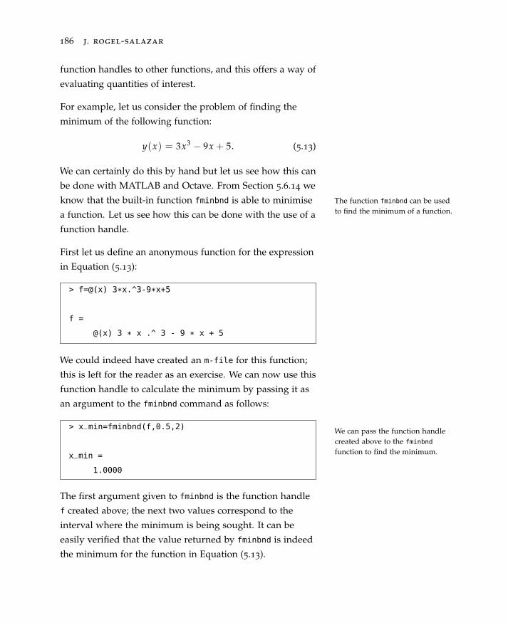
186 j. rogel-salazar

function handles to other functions, and this offers a way of

evaluating quantities of interest.

For example, let us consider the problem of finding the

minimum of the following function:

y(x) = 3x3 − 9x + 5. (5.13)

We can certainly do this by hand but let us see how this can

be done with MATLAB and Octave. From Section 5.6.14 we

know that the built-in function fminbnd is able to minimise The function fminbnd can be usedto find the minimum of a function.a function. Let us see how this can be done with the use of a

function handle.

First let us define an anonymous function for the expression

in Equation (5.13):

> f=@(x) 3*x.^3-9*x+5

f =

@(x) 3 * x .^ 3 - 9 * x + 5

We could indeed have created an m-file for this function;

this is left for the reader as an exercise. We can now use this

function handle to calculate the minimum by passing it as

an argument to the fminbnd command as follows:

We can pass the function handlecreated above to the fminbnd

function to find the minimum.

> x_min=fminbnd(f,0.5,2)

x_min =

1.0000

The first argument given to fminbnd is the function handle

f created above; the next two values correspond to the

interval where the minimum is being sought. It can be

easily verified that the value returned by fminbnd is indeed

the minimum for the function in Equation (5.13).

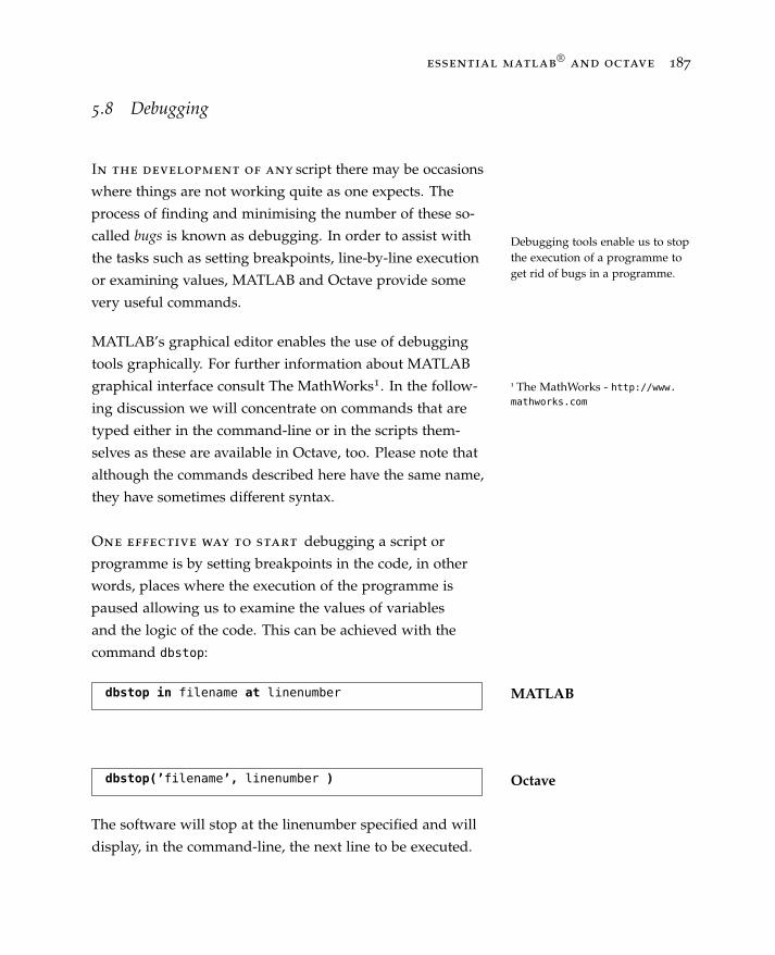
essential matlab®

and octave 187

5.8 Debugging

In the development of any script there may be occasions

where things are not working quite as one expects. The

process of finding and minimising the number of these so-

called bugs is known as debugging. In order to assist with

the tasks such as setting breakpoints, line-by-line execution

or examining values, MATLAB and Octave provide some

very useful commands.

Debugging tools enable us to stopthe execution of a programme toget rid of bugs in a programme.

MATLAB’s graphical editor enables the use of debugging

tools graphically. For further information about MATLAB

graphical interface consult The MathWorks1. In the follow- 1 The MathWorks - http://www.mathworks.coming discussion we will concentrate on commands that are

typed either in the command-line or in the scripts them-

selves as these are available in Octave, too. Please note that

although the commands described here have the same name,

they have sometimes different syntax.

One effective way to start debugging a script or

programme is by setting breakpoints in the code, in other

words, places where the execution of the programme is

paused allowing us to examine the values of variables

and the logic of the code. This can be achieved with the

command dbstop:

MATLABdbstop in filename at linenumber

Octavedbstop(’filename’, linenumber )

The software will stop at the linenumber specified and will

display, in the command-line, the next line to be executed.

188 j. rogel-salazar

In order to let the user know that the debug mode is on,

the prompt will look different. In the case of MATLAB, the

letter K is used at the beginning of the prompt as shown

below:

MATLABK>>

In Octave, the word debug is used as follows:

Octavedebug>

Once the debug mode is on, the software waits until the

user provides input to continue the execution of the pro-

gramme. In order to execute the script one line at a time the

command

dbstep executed the programmeone line at a time.> dbstep

can be used. If instead we want to resume the normal

execution of the script, we can use the command

dbcont resumes the execution ofthe programme.> dbcont

We can leave the debug mode using the command

dbquit quits the debug mode.> dbquit

Let us consider the following function as an example

to debug:

function result = debuggy(x)

n=length(x);

result=n/x;

end

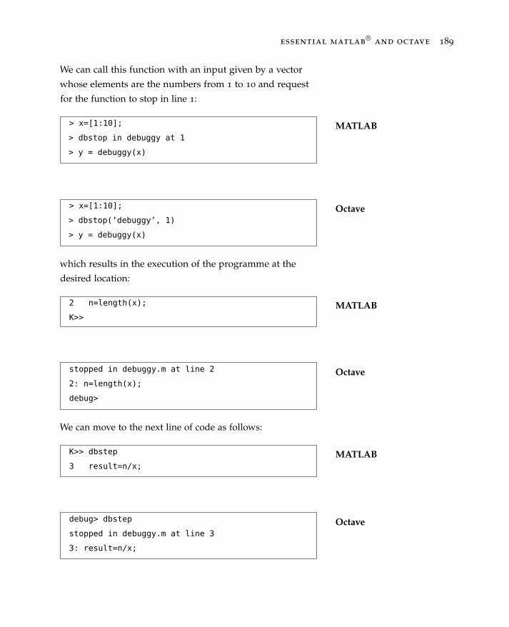
essential matlab®

and octave 189

We can call this function with an input given by a vector

whose elements are the numbers from 1 to 10 and request

for the function to stop in line 1:

MATLAB> x=[1:10];

> dbstop in debuggy at 1

> y = debuggy(x)

Octave> x=[1:10];

> dbstop(’debuggy’, 1)

> y = debuggy(x)

which results in the execution of the programme at the

desired location:

MATLAB2 n=length(x);

K>>

Octavestopped in debuggy.m at line 2

2: n=length(x);

debug>

We can move to the next line of code as follows:

MATLABK>> dbstep

3 result=n/x;

Octavedebug> dbstep

stopped in debuggy.m at line 3

3: result=n/x;

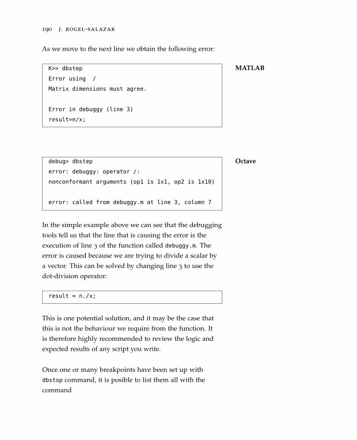
190 j. rogel-salazar

As we move to the next line we obtain the following error:

MATLABK>> dbstep

Error using /

Matrix dimensions must agree.

Error in debuggy (line 3)

result=n/x;

Octavedebug> dbstep

error: debuggy: operator /:

nonconformant arguments (op1 is 1x1, op2 is 1x10)

error: called from debuggy.m at line 3, column 7

In the simple example above we can see that the debugging

tools tell us that the line that is causing the error is the

execution of line 3 of the function called debuggy.m. The

error is caused because we are trying to divide a scalar by

a vector. This can be solved by changing line 3 to use the

dot-division operator:

result = n./x;

This is one potential solution, and it may be the case that

this is not the behaviour we require from the function. It

is therefore highly recommended to review the logic and

expected results of any script you write.

Once one or many breakpoints have been set up with

dbstop command, it is posible to list them all with the

command

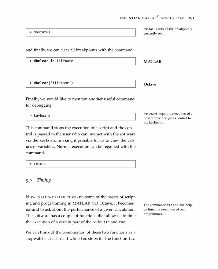
essential matlab®

and octave 191

> dbstatusdbstatus lists all the breakpointscurrently set.

and finally, we can clear all breakpoints with the command

MATLAB> dbclear in filename

Octave> dbclear(’filename’)

Finally, we would like to mention another useful command

for debugging:

keyboard stops the execution of aprogramme and gives control tothe keyboard.

> keyboard

This command stops the execution of a script and the con-

trol is passed to the user who can interact with the software

via the keyboard, making it possible for us to view the val-

ues of variables. Normal execution can be regained with the

command.

> return

5.9 Timing

Now that we have covered some of the basics of script-

ing and programming in MATLAB and Octave, it becomes

natural to ask about the performance of a given calculation.

The software has a couple of functions that allow us to time

the execution of a certain part of the code: tic and toc.

The commands tic and toc helpus time the execution of ourprogrammes.

We can think of the combination of these two functions as a

stopwatch: tic starts it while toc stops it. The function toc

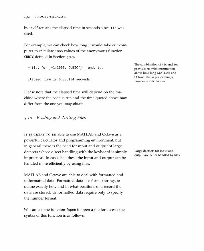
192 j. rogel-salazar

by itself returns the elapsed time in seconds since tic was

used.

For example, we can check how long it would take our com-

puter to calculate 1000 values of the anonymous function

CUBIC defined in Section 5.7.1.

The combination of tic and toc

provides us with informationabout how long MATLAB andOctave take in performing anumber of calculations.

> tic, for j=1:1000, CUBIC(j); end, toc

Elapsed time is 0.005134 seconds.

Please note that the elapsed time will depend on the ma-

chine where the code is run and the time quoted above may

differ from the one you may obtain.

5.10 Reading and Writing Files

It is great to be able to use MATLAB and Octave as a

powerful calculator and programming environment, but

in general there is the need for input and output of large

datasets whose direct handling with the keyboard is simply

impractical. In cases like these the input and output can be

handled more efficiently by using files.

Large datasets for input andoutput are better handled by files.

MATLAB and Octave are able to deal with formatted and

unformatted data. Formatted data use format strings to

define exactly how and in what positions of a record the

data are stored. Unformatted data require only to specify

the number format.

We can use the function fopen to open a file for access; the

syntax of this function is as follows:

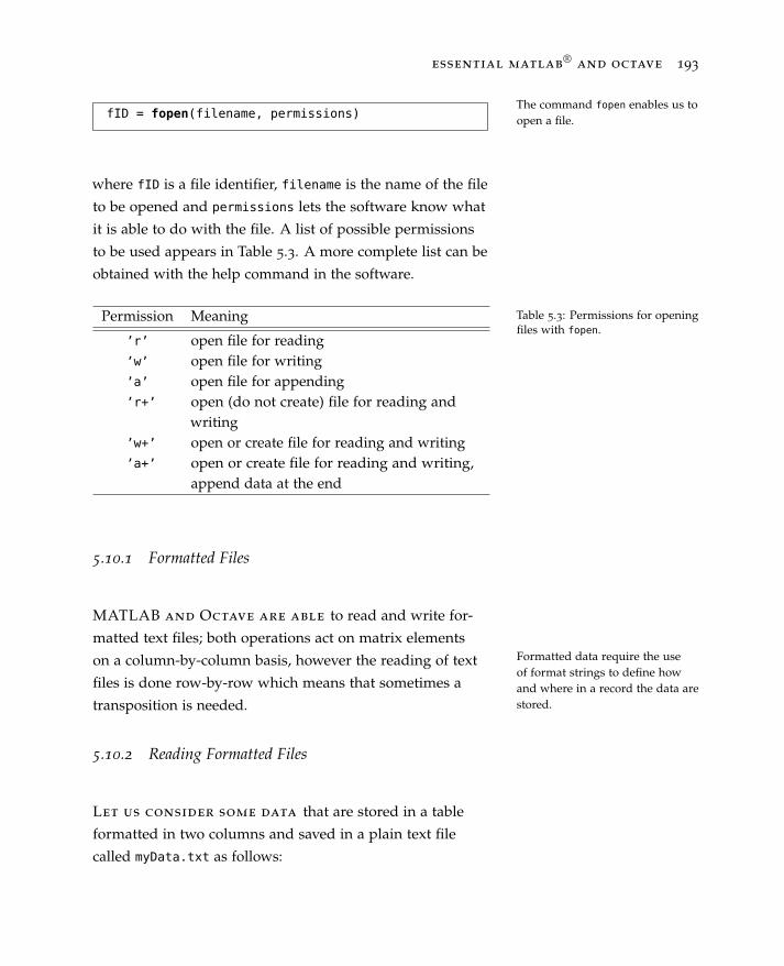
essential matlab®

and octave 193

fID = fopen(filename, permissions)The command fopen enables us toopen a file.

where fID is a file identifier, filename is the name of the file

to be opened and permissions lets the software know what

it is able to do with the file. A list of possible permissions

to be used appears in Table 5.3. A more complete list can be

obtained with the help command in the software.

Permission Meaning

’r’ open file for reading’w’ open file for writing’a’ open file for appending’r+’ open (do not create) file for reading and

writing’w+’ open or create file for reading and writing’a+’ open or create file for reading and writing,

append data at the end

Table 5.3: Permissions for openingfiles with fopen.

5.10.1 Formatted Files

MATLAB and Octave are able to read and write for-

matted text files; both operations act on matrix elements

on a column-by-column basis, however the reading of text

files is done row-by-row which means that sometimes a

transposition is needed.

Formatted data require the useof format strings to define howand where in a record the data arestored.

5.10.2 Reading Formatted Files

Let us consider some data that are stored in a table

formatted in two columns and saved in a plain text file

called myData.txt as follows:

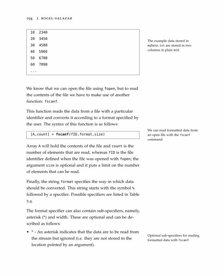
194 j. rogel-salazar

10 2340

20 3450

30 4580

40 5960

50 6788

60 7890

...

The example data stored inmyData.txt are stored in twocolumns in plain text.

We know that we can open the file using fopen, but to read

the contents of the file we have to make use of another

function: fscanf.

This function reads the data from a file with a particular

identifier and converts it according to a format specified by

the user. The syntax of this function is as follows:We can read formatted data froman open file with the fscanf

command.[A,count] = fscanf(fID,format,size)

Array A will hold the contents of the file and count is the

number of elements that are read, whereas fID is the file

identifier defined when the file was opened with fopen; the

argument size is optional and it puts a limit on the number

of elements that can be read.

Finally, the string format specifies the way in which data

should be converted. This string starts with the symbol %

followed by a specifier. Possible specifiers are listed in Table

5.4.

The format specifier can also contain sub-specifiers, namely,

asterisk (*) and width. These are optional and can be de-

scribed as follows:

• * - An asterisk indicates that the data are to be read from

the stream but ignored (i.e. they are not stored in the

location pointed by an argument).

Optional sub-specifiers for readingformatted data with fscanf.

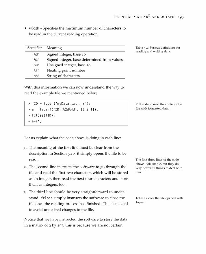
essential matlab®

and octave 195

• width - Specifies the maximum number of characters to

be read in the current reading operation.

Specifier Meaning

’%d’ Signed integer, base 10

’%i’ Signed integer, base determined from values’%u’ Unsigned integer, base 10

’%f’ Floating point number’%s’ String of characters

Table 5.4: Format definitions forreading and writing data.

With this information we can now understand the way to

read the example file we mentioned before:

Full code to read the content of afile with formatted data.

> fID = fopen(’myData.txt’,’r’);

> a = fscanf(fID,’%2d%4d’, [2 inf]);

> fclose(fID);

> a=a’;

Let us explain what the code above is doing in each line:

1. The meaning of the first line must be clear from the

description in Section 5.10: it simply opens the file to be

read. The first three lines of the codeabove look simple, but they dovery powerful things to deal withfiles.

2. The second line instructs the software to go through the

file and read the first two characters which will be stored

as an integer, then read the next four characters and store

them as integers, too.

3. The third line should be very straightforward to under-

stand: fclose simply instructs the software to close the fclose closes the file opened withfopen.file once the reading process has finished. This is needed

to avoid undesired changes to the file.

Notice that we have instructed the software to store the data

in a matrix of 2 by inf; this is because we are not certain

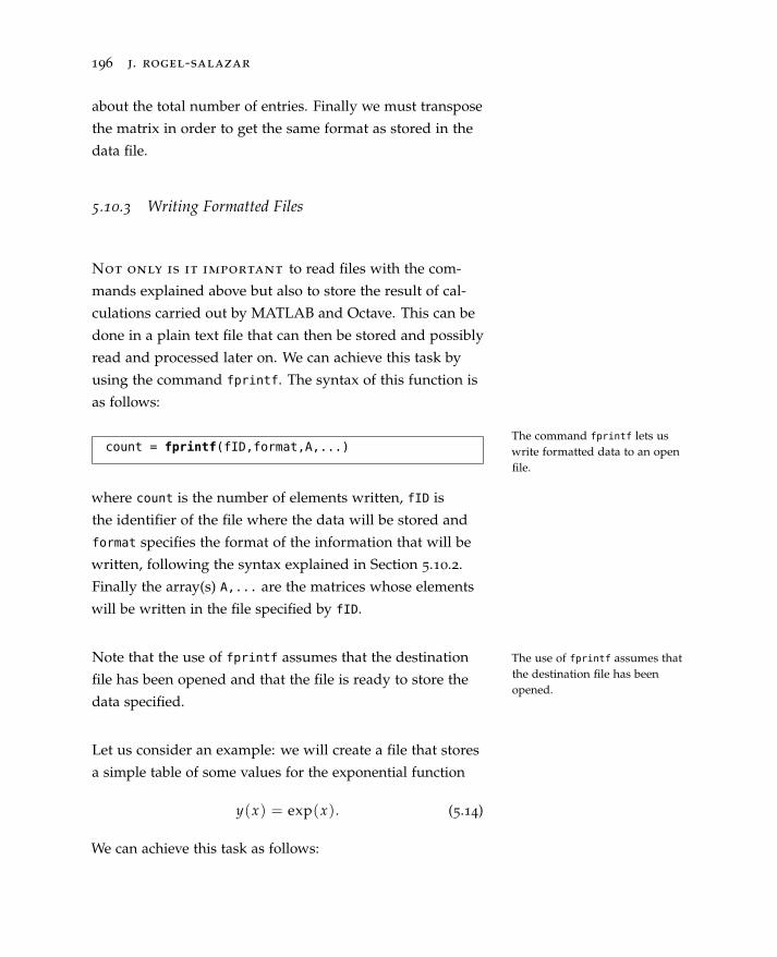
196 j. rogel-salazar

about the total number of entries. Finally we must transpose

the matrix in order to get the same format as stored in the

data file.

5.10.3 Writing Formatted Files

Not only is it important to read files with the com-

mands explained above but also to store the result of cal-

culations carried out by MATLAB and Octave. This can be

done in a plain text file that can then be stored and possibly

read and processed later on. We can achieve this task by

using the command fprintf. The syntax of this function is

as follows:

The command fprintf lets uswrite formatted data to an openfile.

count = fprintf(fID,format,A,...)

where count is the number of elements written, fID is

the identifier of the file where the data will be stored and

format specifies the format of the information that will be

written, following the syntax explained in Section 5.10.2.

Finally the array(s) A,... are the matrices whose elements

will be written in the file specified by fID.

Note that the use of fprintf assumes that the destination The use of fprintf assumes thatthe destination file has beenopened.

file has been opened and that the file is ready to store the

data specified.

Let us consider an example: we will create a file that stores

a simple table of some values for the exponential function

y(x) = exp(x). (5.14)

We can achieve this task as follows:

essential matlab®

and octave 197

> x=0:0.1:1;

> y=[x;exp(x)];

> fid=fopen(’exp.txt’,’w’);

> fprintf(fid,’%6.2f %12.8f\n’,y);

> fclose(fid);

We can generate a file with atabulation of the exponentialfunction with a combination offopen and fprintf.

In the first line we have created a vector with 11 values for

the independent variable x (a sequence from 0 to 1 in steps

of 0.1). We then create an array y whose first column is the

value of x and the second column is the value of exp(x).The third line instructs the software to open a file called

exp.txt; notice that we have passed the argument ’w’ to the

fopen command which implies that the software has writing

permissions. The fourth line stores the values of the matrix

Remember to enable writingpermissions when creating files forstoring data.

y in two columns. Notice that the formatting specifiers

end with the string \n which forces the file to create a new

line and thus the next set of values will be printed in the

next row in the file. Instructions such as \n at the end of

the formatting portion of the command are called controlcharacters and Table 5.5 shows some of the most common

Control characters such as ’\n’enable us to format the data thatwill be stored in the file.

ones.

Specifier Meaning

’\n’ New line’\r’ Beginning of new line’\b’ Backspace’\t’ Tab’\f’ New page

Table 5.5: Control characters usedin formatting output.

Finally, the fifth line closes the file. The result of these

instructions creates a file called exp.txt and its contents are

as follows:

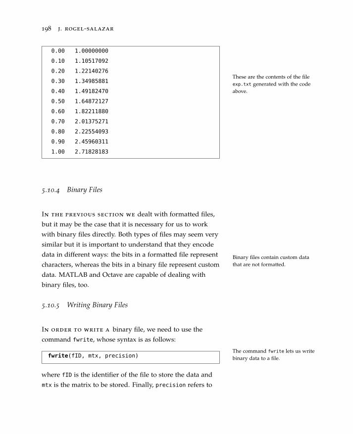
198 j. rogel-salazar

0.00 1.00000000

0.10 1.10517092

0.20 1.22140276

0.30 1.34985881

0.40 1.49182470

0.50 1.64872127

0.60 1.82211880

0.70 2.01375271

0.80 2.22554093

0.90 2.45960311

1.00 2.71828183

These are the contents of the fileexp.txt generated with the codeabove.

5.10.4 Binary Files

In the previous section we dealt with formatted files,

but it may be the case that it is necessary for us to work

with binary files directly. Both types of files may seem very

similar but it is important to understand that they encode

data in different ways: the bits in a formatted file represent

characters, whereas the bits in a binary file represent custom

data. MATLAB and Octave are capable of dealing with

binary files, too.

Binary files contain custom datathat are not formatted.

5.10.5 Writing Binary Files

In order to write a binary file, we need to use the

command fwrite, whose syntax is as follows:

The command fwrite lets us writebinary data to a file.fwrite(fID, mtx, precision)

where fID is the identifier of the file to store the data and

mtx is the matrix to be stored. Finally, precision refers to

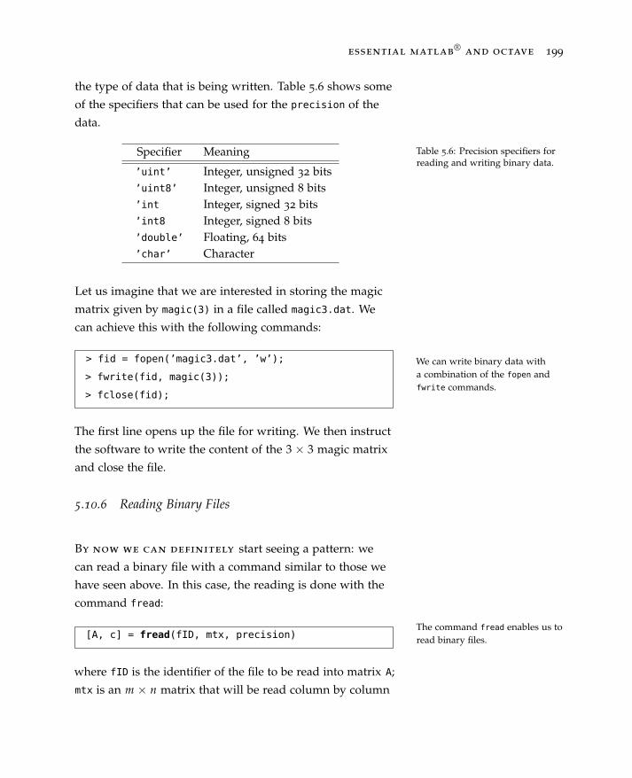
essential matlab®

and octave 199

the type of data that is being written. Table 5.6 shows some

of the specifiers that can be used for the precision of the

data.

Specifier Meaning

’uint’ Integer, unsigned 32 bits’uint8’ Integer, unsigned 8 bits’int Integer, signed 32 bits’int8 Integer, signed 8 bits’double’ Floating, 64 bits’char’ Character

Table 5.6: Precision specifiers forreading and writing binary data.

Let us imagine that we are interested in storing the magic

matrix given by magic(3) in a file called magic3.dat. We

can achieve this with the following commands:

We can write binary data witha combination of the fopen andfwrite commands.

> fid = fopen(’magic3.dat’, ’w’);

> fwrite(fid, magic(3));

> fclose(fid);

The first line opens up the file for writing. We then instruct

the software to write the content of the 3 × 3 magic matrix

and close the file.

5.10.6 Reading Binary Files

By now we can definitely start seeing a pattern: we

can read a binary file with a command similar to those we

have seen above. In this case, the reading is done with the

command fread:

The command fread enables us toread binary files.[A, c] = fread(fID, mtx, precision)

where fID is the identifier of the file to be read into matrix A;

mtx is an m × n matrix that will be read column by column

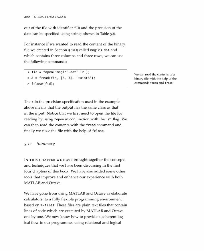
200 j. rogel-salazar

out of the file with identifier fID and the precision of the

data can be specified using strings shown in Table 5.6.

For instance if we wanted to read the content of the binary

file we created in Section 5.10.5 called magic3.dat and

which contains three columns and three rows, we can use

the following commands:

> fid = fopen(’magic3.dat’,’r’);

> A = fread(fid, [3, 3], ’*uint8’);

> fclose(fid);

We can read the contents of abinary file with the help of thecommands fopen and fread.

The * in the precision specification used in the example

above means that the output has the same class as that

in the input. Notice that we first need to open the file for

reading by using fopen in conjunction with the ’r’ flag. We

can then read the contents with the fread command and

finally we close the file with the help of fclose.

5.11 Summary

In this chapter we have brought together the concepts

and techniques that we have been discussing in the first

four chapters of this book. We have also added some other

tools that improve and enhance our experience with both

MATLAB and Octave.

We have gone from using MATLAB and Octave as elaborate

calculators, to a fully flexible programming environment

based on m-files. These files are plain text files that contain

lines of code which are executed by MATLAB and Octave

one by one. We now know how to provide a coherent log-

ical flow to our programmes using relational and logical

essential matlab®

and octave 201

operators. These together with loops and conditional state-

ments enable us to create elaborate procedures that the

software can execute.

Furthermore, we have also seen how functions can give us

the power of carrying out processes in a reproducible way,

with the added advantage of carrying out the calculations

with different parameters (inputs) and obtaining the cor-

responding answers (outputs). In many cases, MATLAB

and Octave already have a number of built-in functions that

can be readily used. Finally, we also discussed the use of

function handles as arguments for other functions.

In the next chapter we will provide a small selection of ex-

amples that showcase some of the capabilities of MATLAB

and Octave.

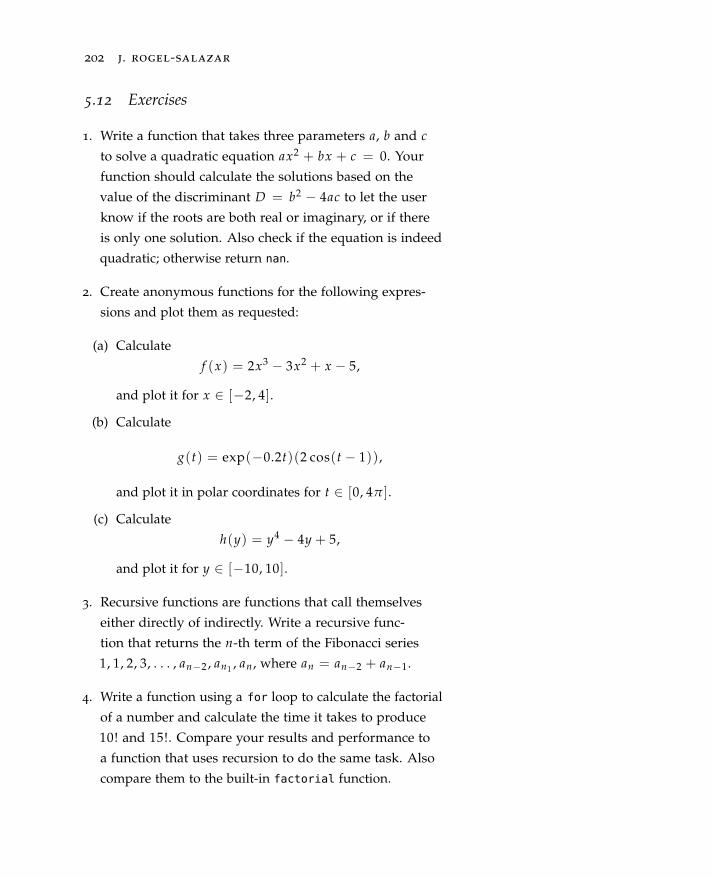
202 j. rogel-salazar

5.12 Exercises

1. Write a function that takes three parameters a, b and cto solve a quadratic equation ax2 + bx + c = 0. Your

function should calculate the solutions based on the

value of the discriminant D = b2 − 4ac to let the user

know if the roots are both real or imaginary, or if there

is only one solution. Also check if the equation is indeed

quadratic; otherwise return nan.

2. Create anonymous functions for the following expres-

sions and plot them as requested:

(a) Calculate

f (x) = 2x3 − 3x2 + x − 5,

and plot it for x ∈ [−2, 4].

(b) Calculate

g(t) = exp(−0.2t)(2 cos(t − 1)),

and plot it in polar coordinates for t ∈ [0, 4π ].

(c) Calculate

h(y) = y4 − 4y + 5,

and plot it for y ∈ [−10, 10].

3. Recursive functions are functions that call themselves

either directly of indirectly. Write a recursive func-

tion that returns the n-th term of the Fibonacci series

1, 1, 2, 3, . . . , an−2 , an1 , an , where an = an−2 + an−1.

4. Write a function using a for loop to calculate the factorial

of a number and calculate the time it takes to produce

10! and 15!. Compare your results and performance to

a function that uses recursion to do the same task. Also

compare them to the built-in factorial function.

essential matlab®

and octave 203

5. Using logical operators create a script that plots the

following function:

g(x) =

{x, −5 ≤ x < 0,

sin(x), 0 ≤ x ≤ 5.

6. Plot the following function

y =sin x

x

for x=−1:0.1:1. Is there something wrong with the plot?

Try sorting the problem using the eps value defined in

the software. After solving the issue, produce a plot in

the interval [−10, 10].

7. Write a script using a while loop that calculates the

successive partial sums

1 +12+

13+ · · · + 1

n

until successive sums are within 0.01 of each other, print-

ing on every step the result of the sum.

8. Using a while loop determine how many terms are

needed for successive sums of 2k to exceed 1000.

9. Write a function that takes the coefficients of a cubic

function

y(x) = ax3 + bx2 + cx + d

and the interval [x1 , x2 ] to create a plot. Your script

should also create a file with the values of x and y.

10. The bisection method is an algorithm to find the root of a

function in a given interval. The method cuts the interval

in two portions and checks which one of them contains

the root by checking for changes of sign in the values of

the function. Pseudo-code for an implementation of the

204 j. rogel-salazar

method is given below. Use the pseudo-code to create a

MATLAB and Octave function for the method.

while (interval [a,b] is not "very small")

{

m=(a+b)/2 % mid-point

if (sign of f(m) is different of sign of f(b))

{ use interval [m,b] in the next iteration

(i.e. replace a with m) }

else

{ use interval [a,m] in the next iteration

(i.e. replace b with m) }

}

approximate root is (a+b)/2

We recommend that you find out what the function feval

does and use it in your implementation. Finally, use your

bisection function to calculate the root of

f (x) = exp(−x) (3.2 sin(x) − 0.5 cos(x))

in the interval [3, 4].

205

6

MATLAB® and Octave in Action

In the previous five chapters we have discussed a

wide range of topics, from what we called “the essential

essentials” of MATLAB and Octave to the usage of various

different objects that the software provides. We have also

highlighted the flexibility that is provided by the scripting

language used by MATLAB and Octave.

In this chapter we present a few examples that showcase the

use of both MATLAB and Octave in context. This should

not be taken as a thorough and rigorous discussion of

the topics used, but rather as a small smörgåsbord that

represents the handling of some of the techniques discussed

earlier on in the book. We therefore recommend reading

The topics and examples pre-sented aim to show the usageof MATLAB and Octave withincontext.

this chapter with the help of a suitable textbook, which may

help clarify some of the concepts and ideas, as well as a

running instance of MATLAB or Octave. We have provided

some basic references in each example with the intention

of guiding you to find further information on each of the

topics addressed. Finally, we would like to encourage you to

try the examples presented here on your own computer; feel

free to adapt the scripts and methods to your own needs.

Try the examples on your owncomputer and start implementingyour own.

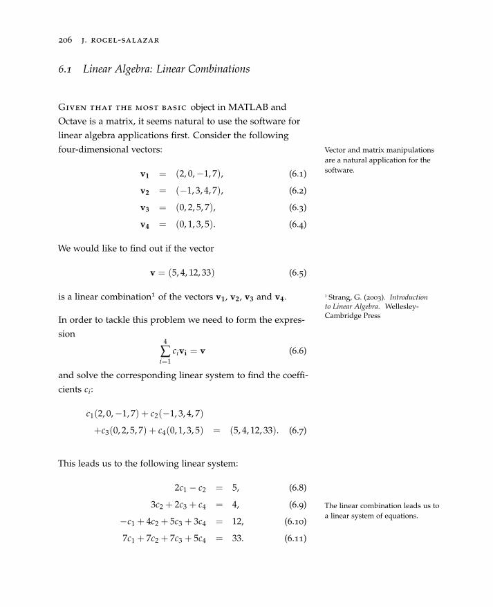
206 j. rogel-salazar

6.1 Linear Algebra: Linear Combinations

Given that the most basic object in MATLAB and

Octave is a matrix, it seems natural to use the software for

linear algebra applications first. Consider the following

four-dimensional vectors: Vector and matrix manipulationsare a natural application for thesoftware.v1 = (2, 0,−1, 7), (6.1)

v2 = (−1, 3, 4, 7), (6.2)

v3 = (0, 2, 5, 7), (6.3)

v4 = (0, 1, 3, 5). (6.4)

We would like to find out if the vector

v = (5, 4, 12, 33) (6.5)

is a linear combination1 of the vectors v1, v2, v3 and v4. 1 Strang, G. (2003). Introductionto Linear Algebra. Wellesley-Cambridge PressIn order to tackle this problem we need to form the expres-

sion4

∑i=1

civi = v (6.6)

and solve the corresponding linear system to find the coeffi-

cients ci:

c1(2, 0,−1, 7) + c2(−1, 3, 4, 7)

+c3(0, 2, 5, 7) + c4(0, 1, 3, 5) = (5, 4, 12, 33). (6.7)

This leads us to the following linear system:

The linear combination leads us toa linear system of equations.

2c1 − c2 = 5, (6.8)

3c2 + 2c3 + c4 = 4, (6.9)

−c1 + 4c2 + 5c3 + 3c4 = 12, (6.10)

7c1 + 7c2 + 7c3 + 5c4 = 33. (6.11)

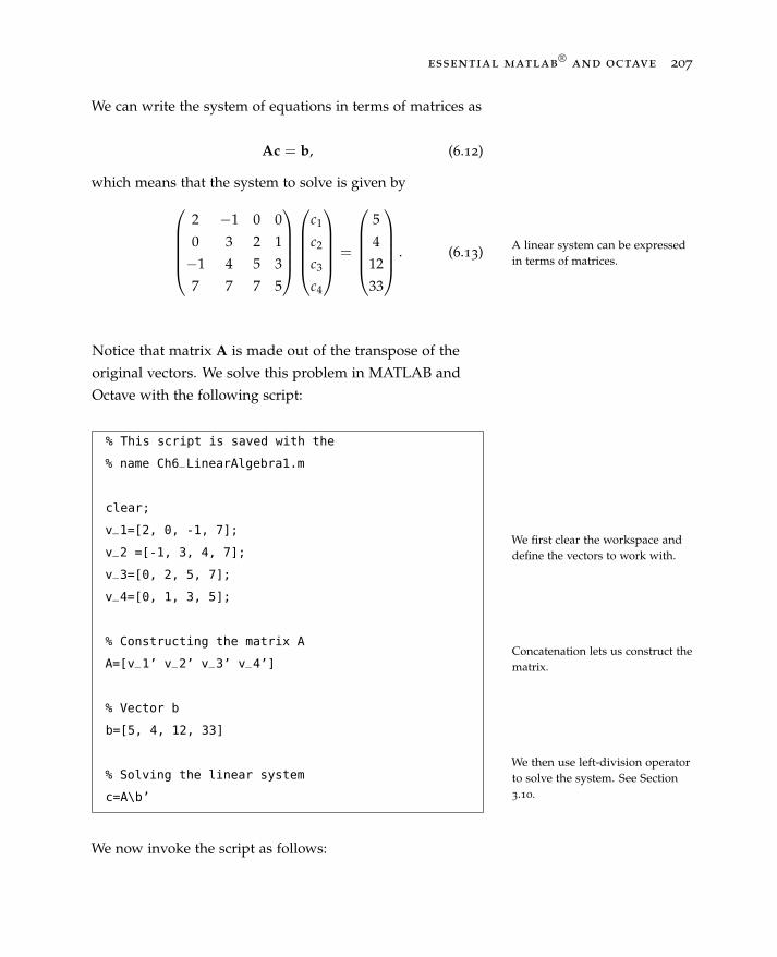
essential matlab®

and octave 207

We can write the system of equations in terms of matrices as

Ac = b, (6.12)

which means that the system to solve is given by

A linear system can be expressedin terms of matrices.

2 −1 0 0

0 3 2 1

−1 4 5 3

7 7 7 5

c1

c2

c3

c4

=

5

4

12

33

. (6.13)

Notice that matrix A is made out of the transpose of the

original vectors. We solve this problem in MATLAB and

Octave with the following script:

We first clear the workspace anddefine the vectors to work with.

Concatenation lets us construct thematrix.

We then use left-division operatorto solve the system. See Section3.10.

% This script is saved with the

% name Ch6_LinearAlgebra1.m

clear;

v_1=[2, 0, -1, 7];

v_2 =[-1, 3, 4, 7];

v_3=[0, 2, 5, 7];

v_4=[0, 1, 3, 5];

% Constructing the matrix A

A=[v_1’ v_2’ v_3’ v_4’]

% Vector b

b=[5, 4, 12, 33]

% Solving the linear system

c=A\b’

We now invoke the script as follows:

208 j. rogel-salazar

> Ch6_LinearAlgebra1

c =

2.00000

-1.00000

3.00000

1.00000

The solution of the linear system isreturned by MATLAB and Octave.

It follows that the system is consistent with the solution

given by

These non-zero values tell us thatthe vector v is a linear combina-tion of the vectors in question.

c1 = 2, (6.14)

c2 = −1, (6.15)

c3 = 3, (6.16)

c4 = 1, (6.17)

and hence v is a linear combination of v1 , v2 , v3 and v4

with

2v1 − v2 + 3v3 + v4 = v. (6.18)

6.2 Linear Algebra: Eigenvalues and Eigenvectors

Let us consider the following 3 × 3 matrix:

A =

3 4 8

1 −3 2

42 15 −4

; (6.19)

we would like to find its eigenvalues and eigenvectors2. 2 Strang, G. (2003). Introductionto Linear Algebra. Wellesley-Cambridge PressWe need to find the values λ that satisfy the characteristic

equation of the matrix A:

det (A− λI) = 0, (6.20)

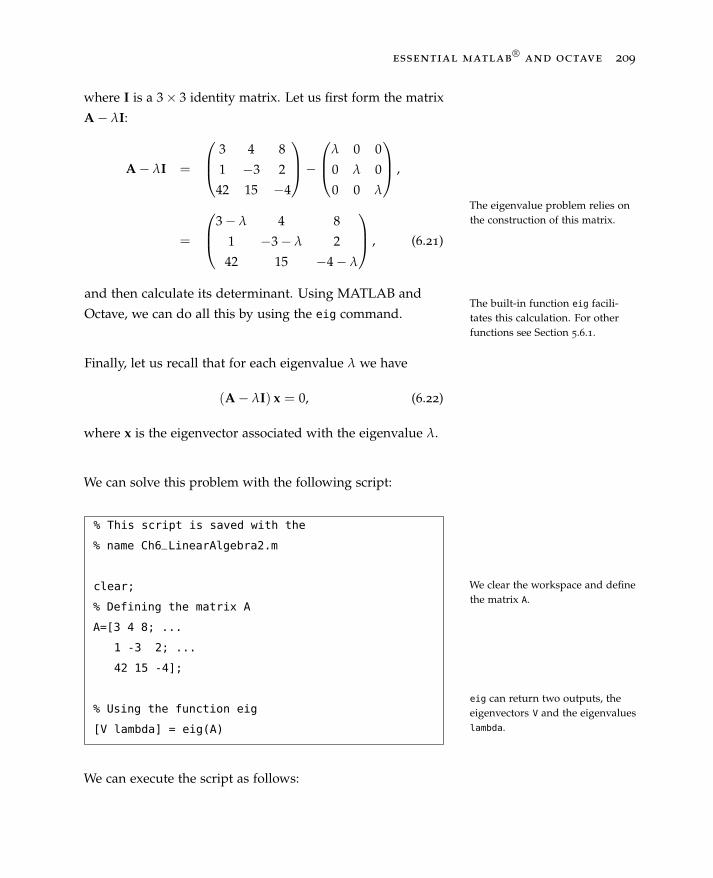
essential matlab®

and octave 209

where I is a 3× 3 identity matrix. Let us first form the matrix

A− λI:

The eigenvalue problem relies onthe construction of this matrix.

A− λI =

3 4 8

1 −3 2

42 15 −4

−λ 0 0

0 λ 0

0 0 λ

,

=

3− λ 4 8

1 −3− λ 2

42 15 −4− λ

, (6.21)

and then calculate its determinant. Using MATLAB and

Octave, we can do all this by using the eig command.The built-in function eig facili-tates this calculation. For otherfunctions see Section 5.6.1.

Finally, let us recall that for each eigenvalue λ we have

(A− λI) x = 0, (6.22)

where x is the eigenvector associated with the eigenvalue λ.

We can solve this problem with the following script:

We clear the workspace and definethe matrix A.

eig can return two outputs, theeigenvectors V and the eigenvalueslambda.

% This script is saved with the

% name Ch6_LinearAlgebra2.m

clear;

% Defining the matrix A

A=[3 4 8; ...

1 -3 2; ...

42 15 -4];

% Using the function eig

[V lambda] = eig(A)

We can execute the script as follows:

210 j. rogel-salazar

> Ch6_LinearAlgebra2

V =

-0.456435 -0.317100 0.331620

-0.099460 -0.094505 -0.925529

-0.884180 0.943672 0.182821

lambda =

Diagonal Matrix

19.3688 0 0

0 -19.6154 0

0 0 -3.7534

The command eig returns a diagonal matrix, lambda, that

The eigenvectors are given by thecolumns of the matrix V.

The eigenvalues are given by thediagonal of the matrix lambda.

contains the eigenvalues, and a matrix V whose columns

correspond to the eigenvectors. This means that the eigen-

values of matrix A in Equation (6.19) are

λ1 = 19.3688, (6.23)

λ2 = −19.6154, (6.24)

λ3 = −3.7534, (6.25)

and the eigenvectors are

These are the eigenvalues ofmatrix A.

These are the eigenvectors ofmatrix A.

v1 =

−0.456435

−0.099460

−0.884180

, (6.26)

v2 =

−0.456435

−0.094505

0.943672

, (6.27)

v3 =

0.331620

−0.925529

0.182821

. (6.28)

essential matlab®

and octave 211

With the aid of Equation (6.22) we can verify that the results

given by MATLAB and Octave are correct. In this case, we

can recast the equation in terms of the eigenvector v1 to

verify that Av1 = λ1v1 :

We can use the colon notation toextract the first eigenvector. SeeSection 3.7.

We can do the same to extract thecorresponding eigenvalue.

We can use matrix multiplicationto calculate the desired results.See Section 3.8.

Finally, we can verify that the twooperations are equal to each other.

> v1= V(:,1)

v1 =

-0.456435

-0.099460

-0.884180

> lambda1=lambda(1,1)

lambda1 =

19.369

> a = A*v1

a =

-8.8406

-1.9264

-17.1255

> b= lambda1*v1

b =

-8.8406

-1.9264

-17.1255

> a-b

ans =

0.0000

0.0000

0.0000

Please note that the formatting used above shows the dif-

ference a−b as zeros, but depending on the format and

212 j. rogel-salazar

precision used you may see a different result but very close

to zero. Finally, similar relationships can be verified for the

other eigenvectors and eigenvalues, i.e. Av2 = λ2v2 and

Av3 = λ3v3 .

6.3 Portfolio Risk: Minimum Variance and Target Port-folios

In this example we will consider a financial portfolio

comprising three assets. In general terms, a portfolio is a

collection of assets, and in turn assets are understood to

be resources with an economic value and which are held

with the expectation that they will provide future benefit

or return. Some examples of assets include stocks, bonds,

funds or even cash. A couple of important measures of

a portfolio are the variance-covariance matrix (Σ) of the

assets, as well as their expected returns. The latter can be

arranged into a column-vector for easier manipulation (R).

The risk associated with a financial portfolio is related to its

standard deviation, given the assets it contains. Investors

are thus interested in balancing the risk of a portfolio and

its expected return3. 3 Elton, E., M. Gruber, S. Brown,and W. Goetzmann (2009). ModernPortfolio Theory and InvestmentAnalysis. John Wiley & SonsFor the purposes of this example we will use the following

variance-covariance matrix:

The variance-covariance matrixis a symmetric matrix. It can becalculated with the cov function.

Σ =

0.3 0.02 −0.05

0.02 0.4 0.06

−0.05 0.06 0.6

, (6.29)

and the vector of expected returns is given by

R =

0.1

0.12

0.14

. (6.30)

essential matlab®

and octave 213

6.3.1 Minimum Variance Portfolio

Let us calculate the weights that will provide us with

a portfolio with minimum risk. As mentioned above, the

risk of the portfolio is related to the standard deviation and

it can be calculated as follows4: 4 Elton, E., M. Gruber, S. Brown,and W. Goetzmann (2009). ModernPortfolio Theory and InvestmentAnalysis. John Wiley & Sonsσ =

√XTΣX, (6.31)

where X is a vector whose elements represent the weight on

each of the assets in the portfolio. The expected return of

the portfolio is given byThe superscript T denotes thetranspose operation. See Section3.2.

Rp = XTR. (6.32)

We obtain the minimum variance portfolio by solving the

following optimisation problem:

min XTΣX

subject to: (6.33)

∑ iXi = 1,

where XTΣX is the variance of the portfolio and we are

The weights Xi can be thought ofas the percentages invested in eachasset and thus they must add upto 100%.

using the constraint that the weights of the portfolio add up

to 1.

We solve this problem using Lagrange multipliers to min-

imise the variance. In the case of the variance-covariance

matrix shown in Equation (6.29) this leads us to the follow-

ing linear system: Lagrange multipliers is a popularoptimisation technique findinglocal maxima or minima of afunction subject to equalityconstraints.

0.6 0.04 −0.1 −1

0.04 0.8 0.12 −1

−0.1 0.12 1.2 −1

1 1 1 0

x1

x2

x3

λ

=

0

0

0

1

. (6.34)

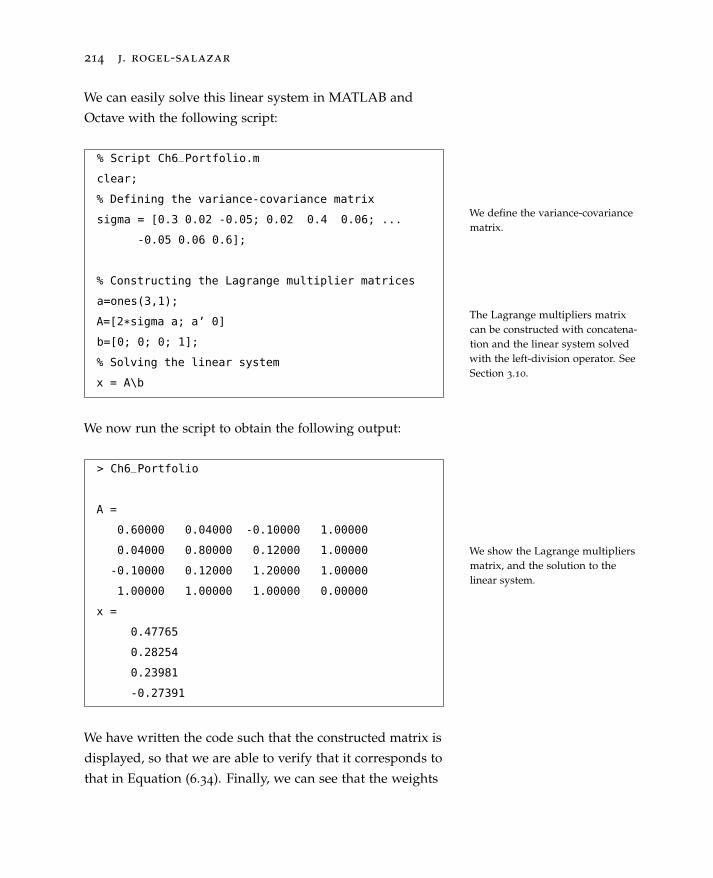
214 j. rogel-salazar

We can easily solve this linear system in MATLAB and

Octave with the following script:

We define the variance-covariancematrix.

The Lagrange multipliers matrixcan be constructed with concatena-tion and the linear system solvedwith the left-division operator. SeeSection 3.10.

% Script Ch6_Portfolio.m

clear;

% Defining the variance-covariance matrix

sigma = [0.3 0.02 -0.05; 0.02 0.4 0.06; ...

-0.05 0.06 0.6];

% Constructing the Lagrange multiplier matrices

a=ones(3,1);

A=[2*sigma a; a’ 0]

b=[0; 0; 0; 1];

% Solving the linear system

x = A\b

We now run the script to obtain the following output:

We show the Lagrange multipliersmatrix, and the solution to thelinear system.

> Ch6_Portfolio

A =

0.60000 0.04000 -0.10000 1.00000

0.04000 0.80000 0.12000 1.00000

-0.10000 0.12000 1.20000 1.00000

1.00000 1.00000 1.00000 0.00000

x =

0.47765

0.28254

0.23981

-0.27391

We have written the code such that the constructed matrix is

displayed, so that we are able to verify that it corresponds to

that in Equation (6.34). Finally, we can see that the weights

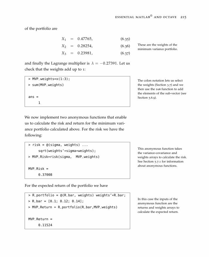
essential matlab®

and octave 215

of the portfolio are

X1 = 0.47765, (6.35)

X2 = 0.28254, (6.36)

X3 = 0.23981, (6.37)

and finally the Lagrange multiplier is λ = −0.27391. Let us

These are the weights of theminimum variance portfolio.

check that the weights add up to 1:

The colon notation lets us selectthe weights (Section 3.7) and wethen use the sum function to addthe elements of the sub-vector (seeSection 5.6.9).

> MVP_weights=x(1:3);

> sum(MVP_weights)

ans =

1

We now implement two anonymous functions that enable

us to calculate the risk and return for the minimum vari-

ance portfolio calculated above. For the risk we have the

following:

This anonymous function takesthe variance-covariance andweights arrays to calculate the risk.See Section 5.7.1 for informationabout anonymous functions.

> risk = @(sigma, weights) ...

sqrt(weights’*sigma*weights);

> MVP_Risk=risk(sigma, MVP_weights)

MVP_Risk =

0.37008

For the expected return of the portfolio we have

In this case the inputs of theanonymous function are thereturns and weights arrays tocalculate the expected return.

> R_portfolio = @(R_bar, weights) weights’*R_bar;

> R_bar = [0.1; 0.12; 0.14];

> MVP_Return = R_portfolio(R_bar,MVP_weights)

MVP_Return =

0.11524

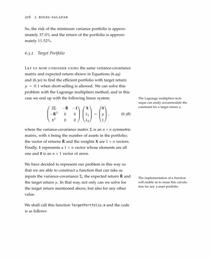
216 j. rogel-salazar

So, the risk of the minimum variance portfolio is approx-

imately 37.0% and the return of the portfolio is approxi-

mately 11.52%.

6.3.2 Target Portfolio

Let us now consider using the same variance-covariance

matrix and expected return shown in Equations (6.29)

and (6.30) to find the efficient portfolio with target return

µ = 0.1 when short-selling is allowed. We can solve this

problem with the Lagrange multipliers method, and in this

case we end up with the following linear system: The Lagrange multipliers tech-nique can easily accommodate theconstraint for a target return µ. 2Σ −R −1

−RT 0 0

1T 0 0

X

λ1

λ2

=

0µ

1

, (6.38)

where the variance-covariance matrix Σ is an n× n symmetric

matrix, with n being the number of assets in the portfolio;

the vector of returns R and the weights X are 1× n vectors.

Finally, 1 represents a 1× n vector whose elements are all

one and 0 is an n× 1 vector of zeros.

We have decided to represent our problem in this way so

that we are able to construct a function that can take as

inputs the variance-covariance Σ, the expected return R and

the target return µ. In that way, not only can we solve for

the target return mentioned above, but also for any other

value.

The implementation of a functionwill enable us to reuse this calcula-tion for any 3-asset portfolio.

We shall call this function TargetPortfolio.m and the code

is as follows:

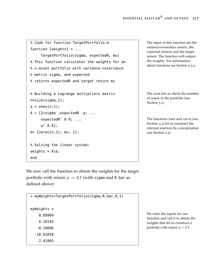
essential matlab®

and octave 217

The input of this function are thevariance-covariance matrix, theexpected returns and the targetreturn. The function will outputthe weights. For informationabout functions see Section 5.5.2.

The size lets us check the numberof assets in the portfolio (seeSection 3.1).

The functions ones and zeros (seeSection 3.3) let us construct therelevant matrices by concatenation(see Section 3.5).

% Code for function TargetPortfolio.m

function [weights] = ...

TargetPortfolio(sigma, expectedR, mu)

% This function calculates the weights for an

% n-asset portfolio with variance-covariance

% matrix sigma, and expected

% returns expectedR and target return mu

% Building a Lagrange multipliers matrix

n=size(sigma,1);

a = ones(n,1);

A = [2*sigma -expectedR -a; ...

expectedR’ 0 0; ...

a’ 0 0];

b= [zeros(n,1); mu; 1];

% Solving the linear system:

weights = A\b;

end

We now call the function to obtain the weights for the target

portfolio with return µ = 0.1 (with sigma and R_bar as

defined above):

We enter the inputs for ourfunction and call it to obtain theweights that let us construct aportfolio with return µ = 0.1.

> myWeights=TargetPortfolio(sigma,R_bar,0.1)

myWeights =

0.89904

0.20192

-0.10096

-18.61058

2.41865

218 j. rogel-salazar

The weights are thus given by

These are the weights for a targetportfolio with µ = 0.1.

X1 = 0.89904, (6.39)

X2 = 0.20192, (6.40)

X3 = −0.10096, (6.41)

and finally the Lagrange multipliers are λ1 = −18.61058

and λ2 = 2.41865. We could check that the weights ob-

tained indeed add up to one:

As before, we can use the colonnotation and the sum function toverify that the weights add up to1.

> Target_weights = myWeights(1:3);

> sum(Target_weights)

ans =

1

We finally use the anonymous functions defined above to

calculate the risk and return of this target portfolio:

> Target_risk = risk(sigma, Target_weights)

Target_risk =

0.52801

> Target_return=R_portfolio(R_bar, Target_weights)

Target_return =

0.10000

As we can see, the risk associated with this target portfolio

The anonymous functions risk

and R_Portfolio can be re-usedto calculate the risk and return forthis portfolio.

We can thus verify that theweights calculated create a portfo-lio with return µ = 0.1.

is σ = 53.8% and we corroborate that the weights calculated

indeed imply a return of µ = 10%.

essential matlab®

and octave 219

6.4 Differential Equations: Predator-Prey Model

Differential equations find applications in a large

number of areas, ranging from physics to biology. In this

case let us take a look at a predator-prey model5 based 5 Britton, N. (2003). EssentialMathematical Biology. SpringerUndergraduate MathematicsSeries. Springer London

on the Lotka-Volterra equations for a prey population, say

rabbits, R(t) and a predator population, say foxes, F(t):

dRdt

= rR− αRF, (6.42)

dFdt

= −δF + βRF. (6.43)

The model above assumes that without foxes, i.e. when

F(t) = 0, the rabbit population grows exponentially at a rate

r:dRdt

= rR; (6.44)

similarly, without rabbits (R(t) = 0) the fox population

decreases exponentially at a rate δ:

dFdt

= −δF. (6.45)

The interaction of the prey and predator populations

is represented by the terms that contain RF, having on the

one hand a negative impact on the rabbits, and on the other

a positive impact on the foxes. We are interested in using

MATLAB and Octave to model the change in size of the

rabbit and fox populations, together, over time.

MATLAB and Octave are able tosolve initial value problems withbuilt-in functions such as ode45 inMATLAB and lsode in Octave.

Furthermore, we shall assign the following values to the

different parameters in Equations (6.42) and (6.43): r = 1.2,

α = 2.5, δ = −0.5 and β = 0.6. Also we will need the initial

220 j. rogel-salazar

values for the rabbit and fox populations: R(0) = 80 and

F(0) = 100.

MATLAB and Octave are able to solve the system

of ordinary differential equations (ODEs) shown above

by using, for instance, a built-in implementation of the

Runge-Kutta method. In MATLAB, we can use the function

ode45. Please note that MATLAB has a number of other ode45 is an implementation of theRunge-Kutta method of order 4.solvers and they are used in a very similar fashion to the

one highlighted here.

The usage of the ode45 function is as follows:

MATLAB[t,y] = ode45(@f_handle, [t0,tf], initial_vals)

where @f_handle is a handle to a function that defines the

differential equations to be solved, [t0,tf] is a vector that

defines the initial and final values of the time variable t and

finally initial_vals is a vector with the initial conditions

for the spatial vector y.

Octave does not have an implementation of ode45; instead

you can use the lsode function. The inputs that lsode

lsode can be used in Octave tosolve stiff ordinary differentialequations.

expects are similar to those passed to MATLAB’s ode45. Let

us take a look:

Octave[y] = lsode(@f_handle, initial_vals, t_interval)

As we can see the variables are the same as defined above,

and t_interval is a vector that defines the time interval.

Notice that the order of the input for ode45 and lsode

is different and this is an important point, as this has an

impact on the script that defines the function handle to be

passed to lsode compared to that passed to ode45.

Octave’s lsode requires the inputsin reverse order to MATLAB’sode45.

essential matlab®

and octave 221

Before tackling the solution of the coupled system of dif-

ferential equations, let us rewrite our model in a vectorised

form: we define a vector v whose first component v1 refers

to the rabbit population whereas the second component v2

refers to the fox one:

It is important to express thesystem of ordinary differentialequations in terms of matrices.This will be needed to define afunction for MATLAB and Octaveto use an input.

dvdt

=ddt

[v1

v2

],

=

[dRdtdFdt

],

=

[1.2R − 2.5RF−0.5F + 0.6RF

]. (6.46)

We will use this vectorised form of our problem to write

a function that implements the model given by Equations

(6.42) and (6.43). The function that defines the ODE system

in MATLAB is a bit different to the one in Octave.

6.4.1 Ordinary Differential Equation System in MATLAB

We need to define a function that implements the ODE

system and which can be passed as a handle to ode45. You

are encouraged to take a look at the help offered for this

function by typing help ode45. In a nutshell, this function

expects a definition where the input for the time variable t

is given first, and then the space vector (v in our case).

Remember that MATLAB expectsthe independent variable t firstand then the dependent variablesin vector form.

With this in mind, let us create a function script which we

will call predator_prey_matlab.m:

222 j. rogel-salazar

MATLABfunction dv = predator_prey_matlab(t,v)

% This function calculates

% the Lotka-Volterra equations

% for predator-prey modelling

% for use in MATLAB

% dR/dt = 0.5R - 0.01 R*F

% dF/dt = -0.5R + 0.01 R*F

% Using a vectorised version where

% v=[v(1) v(2)]=[R F]

% Initialise the vector dv with zeros:

dv=zeros(2,1);

% Calculate dR/dt

dv(1) = 0.5*v(1) - 0.01*v(1)*v(2);

% Calculate dF/dt

dv(2) = -0.5*v(2) + 0.01*v(1)*v(2);

end

In the function above we have defined a vector dv whose

The function will return a vectorwhose entries are given by theODEs in question. For functiondefinitions see Section 5.5.2.

We first initialise the elementswith zeros (see Section 3.3).

Finally, we implement each of theODEs in the system.

entries dv(1) and dv(2) hold the values for dR(t)dt and dF(t)

dt .

We initialise the vector with zeros and assign to each compo-

nent Equations (6.42) and (6.43), respectively.

6.4.2 Ordinary Differential Equation System in Octave

The function that will be used for lsode requires

that the space vector v is passed first, followed by the time

variable t. As such, the only thing we need to change

Octave expects a function wherethe dependent variables are firstand then the independent variablet.

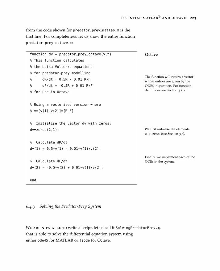
essential matlab®

and octave 223

from the code shown for predator_prey_matlab.m is the

first line. For completeness, let us show the entire function

predator_prey_octave.m:

Octavefunction dv = predator_prey_octave(v,t)

% This function calculates

% the Lotka-Volterra equations

% for predator-prey modelling

% dR/dt = 0.5R - 0.01 R*F

% dF/dt = -0.5R + 0.01 R*F

% for use in Octave

% Using a vectorised version where

% v=[v(1) v(2)]=[R F]

% Initialise the vector dv with zeros:

dv=zeros(2,1);

% Calculate dR/dt

dv(1) = 0.5*v(1) - 0.01*v(1)*v(2);

% Calculate dF/dt

dv(2) = -0.5*v(2) + 0.01*v(1)*v(2);

end

The function will return a vectorwhose entries are given by theODEs in question. For functiondefinitions see Section 5.5.2.

We first initialise the elementswith zeros (see Section 3.3).

Finally, we implement each of theODEs in the system.

6.4.3 Solving the Predator-Prey System

We are now able to write a script, let us call it SolvingPredatorPrey.m,

that is able to solve the differential equation system using

either ode45 for MATLAB or lsode for Octave.

224 j. rogel-salazar

Let us start by defining useful parameters for this problem

as follows:

To allow for flexibility in usingMATLAB and Octave, we imple-ment the control variable mlab todecide if we are running the codein MATLAB or Octave.

We define initial and final timesfor the solution.

Similarly, we define the initialvalues.

% Script SolvingPredatorPrey.m:

% Solve the system of ODEs defined in

% the function predator_prey...

% If mlab = 1 we are using MATLAB

% otherwise we are using Octave.

mlab = 1;

% Define initial and final times

t0 = 0;

tf = 50;

n=1000;

% Used in Octave only

t_interval = linspace(t0,tf,n);

% Define initial values vector

% with R(0) = 80, and F(0) = 100

initial_vals = [80; 100];

The script SolvingPredatorPrey.m is written in such a

way that it can be used with either of the two ODE system

definitions shown in the previous sections. We are able to

do so with the use of a control variable; in this case we call

this variable mlab: when mlab is equal to 1 we implement

the solution using MATLAB’s ode45; for any other value

(0 for example) the solution will be found using Octave’s

lsode. We now proceed to solve the system:

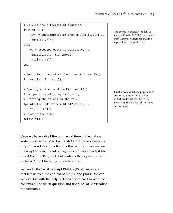
essential matlab®

and octave 225

% Solving the differential equations

if mlab == 1

[t,v] = ode45(@predator_prey_matlab,[t0,tf],...

initial_vals);

else

[v] = lsode(@predator_prey_octave, ...

initial_vals, t_interval);

t=t_interval’;

end

% Returning to original functions R(t) and F(t)

R = v(:,1); F = v(:,2);

% Opening a file to store R(t) and F(t)

fid=fopen(’PredatorPrey.txt’,’w’);

% Printing the values to the file

fprintf(fid,’%12.8f %12.8f %12.8f\n’, ...

[t’; R’; F’]);

% Closing the file

fclose(fid);

The control variable mlab lets ususe ode45 with MATLAB or lsodewith Octave. Remember that theinputs have different order.

Finally, we extract the populationsand write the results to a filecalled PredatorPrey.txt withthe aid of fopen and fprintf. SeeSection 5.10.

Once we have solved the ordinary differential equation

system with either MATLAB’s ode45 or Octave’s lsode we

output the solution to a file. In other words, when we run

the script SolvingPredatorPrey.m we will obtain a text file

called PredatorPrey.txt that contains the population for

rabbit R(t) and foxes F(t) at each time t.

We can further write a script PlottingPredatorPrey.m

that lets us read the content of the file and plot it. We can

achieve this with the help of fopen and fscanf to read the

contents of the file in question and use subplot to visualise

the functions:

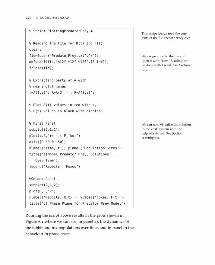
226 j. rogel-salazar

% Script PlottingPredatorPrey.m

% Reading the file for R(t) and F(t)

clear;

fid=fopen(’PredatorPrey.txt’,’r’);

A=fscanf(fid,’%12f %12f %12f’,[3 inf]);

fclose(fid);

% Extracting parts of A with

% meaningful names

t=A(1,:)’; R=A(2,:)’; F=A(3,:)’;

% Plot R(t) values in red with *,

% F(t) values in black with circles.

% First Panel

subplot(2,1,1);

plot(t,R,’r*-’,t,F,’ko:’)

axis([0 50 0 150]);

xlabel(’Time, t’); ylabel(’Population Sizes’);

title(’a)Model Predator Prey, Solutions ...

Over Time’)

legend(’Rabbits’,’Foxes’)

%Second Panel

subplot(2,1,2);

plot(R,F,’k’)

xlabel(’Rabbits, R(t)’); ylabel(’Foxes, F(t)’);

title(’b) Phase Plane for Predator Prey Model’)

Running the script above results in the plots shown in

This script lets us read the con-tents of the file PredatorPrey.txt.

We assign an id to the file andopen it with fopen. Reading canbe done with fscanf. See Section5.10.

We can now visualise the solutionto the ODE system with thehelp of subplot. See Sectionsec:subplots.

Figure 6.1 where we can see, in panel a), the dynamics of

the rabbit and fox populations over time, and in panel b) the

behaviour in phase space.

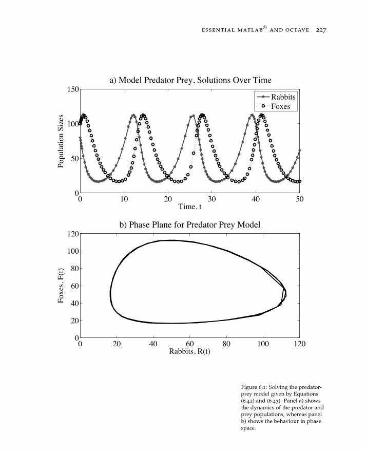
essential matlab®

and octave 227

0 10 20 30 40 500

50

100

150

Time, t

Popu

latio

n Si

zes

a) Model Predator Prey, Solutions Over Time

RabbitsFoxes

0 20 40 60 80 100 1200

20

40

60

80

100

120

Rabbits, R(t)

Foxe

s, F(

t)

b) Phase Plane for Predator Prey Model

Figure 6.1: Solving the predator-prey model given by Equations(6.42) and (6.43). Panel a) showsthe dynamics of the predator andprey populations, whereas panelb) shows the behaviour in phasespace.

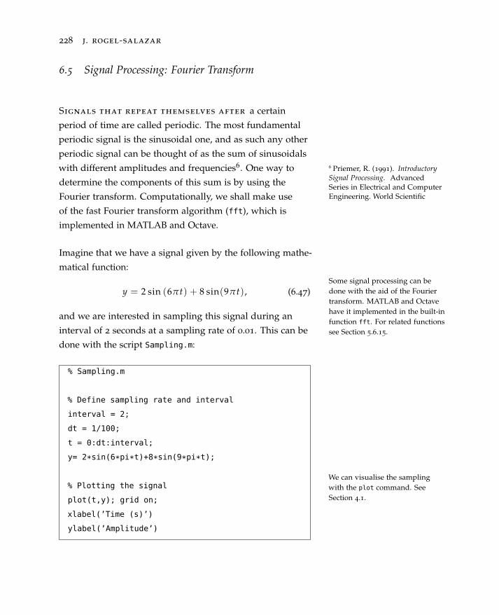
228 j. rogel-salazar

6.5 Signal Processing: Fourier Transform

Signals that repeat themselves after a certain

period of time are called periodic. The most fundamental

periodic signal is the sinusoidal one, and as such any other

periodic signal can be thought of as the sum of sinusoidals

with different amplitudes and frequencies6. One way to 6 Priemer, R. (1991). IntroductorySignal Processing. AdvancedSeries in Electrical and ComputerEngineering. World Scientific

determine the components of this sum is by using the

Fourier transform. Computationally, we shall make use

of the fast Fourier transform algorithm (fft), which is

implemented in MATLAB and Octave.

Imagine that we have a signal given by the following mathe-

matical function:Some signal processing can bedone with the aid of the Fouriertransform. MATLAB and Octavehave it implemented in the built-infunction fft. For related functionssee Section 5.6.15.

y = 2 sin (6π t) + 8 sin(9π t), (6.47)

and we are interested in sampling this signal during an

interval of 2 seconds at a sampling rate of 0.01. This can be

done with the script Sampling.m:

We can visualise the samplingwith the plot command. SeeSection 4.1.

% Sampling.m

% Define sampling rate and interval

interval = 2;

dt = 1/100;

t = 0:dt:interval;

y= 2*sin(6*pi*t)+8*sin(9*pi*t);

% Plotting the signal

plot(t,y); grid on;

xlabel(’Time (s)’)

ylabel(’Amplitude’)

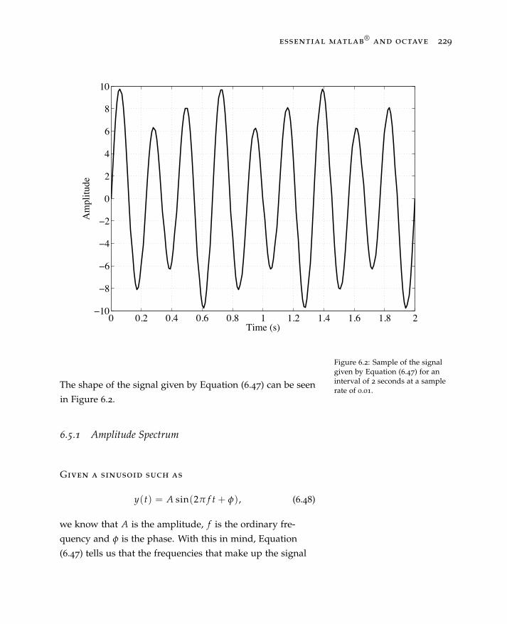
essential matlab®

and octave 229

0 0.2 0.4 0.6 0.8 1 1.2 1.4 1.6 1.8 2ï10

ï8

ï6

ï4

ï2

0

2

4

6

8

10

Time (s)

Am

plitu

de

Figure 6.2: Sample of the signalgiven by Equation (6.47) for aninterval of 2 seconds at a samplerate of 0.01.

The shape of the signal given by Equation (6.47) can be seen

in Figure 6.2.

6.5.1 Amplitude Spectrum

Given a sinusoid such as

y(t) = A sin(2π f t + φ), (6.48)

we know that A is the amplitude, f is the ordinary fre-

quency and φ is the phase. With this in mind, Equation

(6.47) tells us that the frequencies that make up the signal

230 j. rogel-salazar

y are thus 3 Hz and 4.5 Hz, and that the amplitudes of the

original signals are 2 and 8, respectively. We can identify

these amplitudes and frequencies by calculating the ampli-

tude spectrum of the signal using the Fourier transform:

The amplitude spectrum revealsthe main frequencies that make upthe signal.

We take the Fourier transform ofthe signal with fft and a normal-isation constant is calculated. Formore information check the help

for this function.

We then plot the amplitudespectrum with plot.

% AmplitudeSpectrum.m

% Given the signal y calculate the FFT

Y=fft(y);

% Calculate the normalisation constant

n=size(y,2)/2;

% Take the abs value and normalise

spectrum=abs(Y)/n;

% Plotting the FFT

frequencies = (0:14)/(2*n*dt);

plot(frequencies, spectrum(1:15)); grid on

xlabel(’Frequency (Hz)’);

ylabel(’Amplitude’);

The plot generated with the script above can be seen in Fig-

ure 6.3 where we are able to clearly distinguish two peaks,

one at 2 Hz and the other at 4 Hz as expected. Furthermore,

the heights of the peaks indicate the amplitudes of the

original sinusoidal signals.

6.5.2 Noise Filtering

The Fourier transform used in the example above

can be used to filter out noise from a signal. Let us con-

sider adding some random noise to the signal y given by

Equation (6.47):

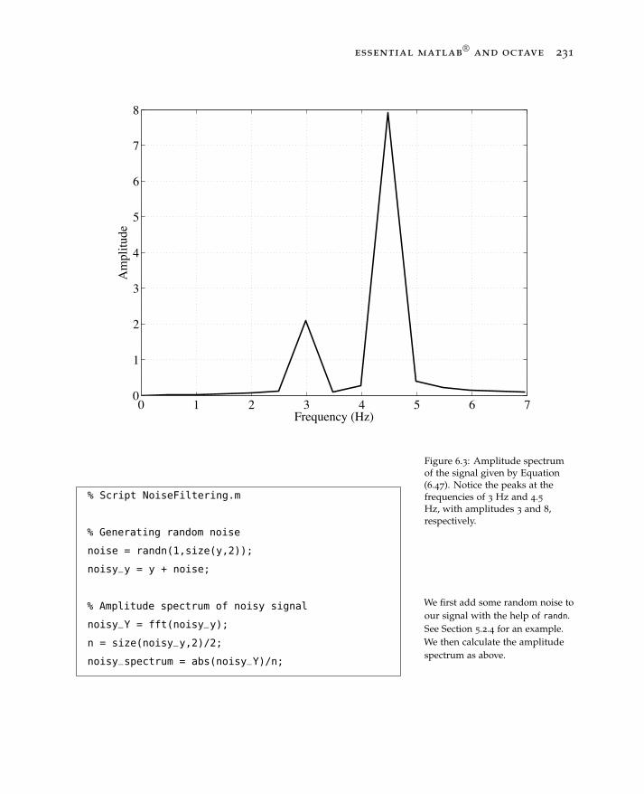
essential matlab®

and octave 231

0 1 2 3 4 5 6 70

1

2

3

4

5

6

7

8

Frequency (Hz)

Am

plitu

de

Figure 6.3: Amplitude spectrumof the signal given by Equation(6.47). Notice the peaks at thefrequencies of 3 Hz and 4.5Hz, with amplitudes 3 and 8,respectively.

% Script NoiseFiltering.m

% Generating random noise

noise = randn(1,size(y,2));

noisy_y = y + noise;

% Amplitude spectrum of noisy signal

noisy_Y = fft(noisy_y);

n = size(noisy_y,2)/2;

noisy_spectrum = abs(noisy_Y)/n;

We first add some random noise toour signal with the help of randn.See Section 5.2.4 for an example.We then calculate the amplitudespectrum as above.

232 j. rogel-salazar

We can add to our script a few commands to visualise the

noisy signal and its amplitude spectrum:

The command subplot enablesto visualise both the noisy signaland its frequency spectrum. SeeSection 4.5.

% Plotting noisy signal

figure(1)

subplot(2,1,1);

plot(time,noisy_y); grid on

title(’a) Signal with random noise’);

xlabel(’Time (s)’);

ylabel(’Amplitude’);

% Plotting amplitude spectrum

subplot(2,1,2);

noisy_freq = (0:14)/(2*n*dt);

plot(noisy_freq,noisy_spectrum(1:15)); grid on

title(’b) Amplitude spectrum of noisy signal’);

xlabel(’Frequency (Hz)’);

ylabel(’Amplitude’);

The result of adding noise to our signal can be seen in panel

a) of Figure 6.4. We can compare this to the signal shown in

Figure 6.2 and observe that they share some characteristics.

In order to convince ourselves that the main frequencies

are the same, we plot the amplitude spectrum of the noisy

signal in panel b) of Figure 6.4 where we can see the same

peaks that we have observed before.

The amplitude spectrum of thenoisy signal shows its main fre-quencies enabling us to implementa filter.

Finally, let us use the inverse Fourier transform to filter out

the low amplitude noise to correct the signal. We do this

by eliminating those points that are above a cut off value in

amplitude:

essential matlab®

and octave 233

0 0.5 1 1.5 2ï20

ï10

0

10

20a) Signal with random noise

Time (s)

Am

plitu

de

0 1 2 3 4 5 6 70

2

4

6

8b) Amplitude spectrum of noisy signal

Frequency (Hz)

Am

plitu

de

Figure 6.4: Panel a) Noisy signalgenerated by adding randomnoise to original sampling. Panelb) Amplitude spectrum of thenoisy signal.

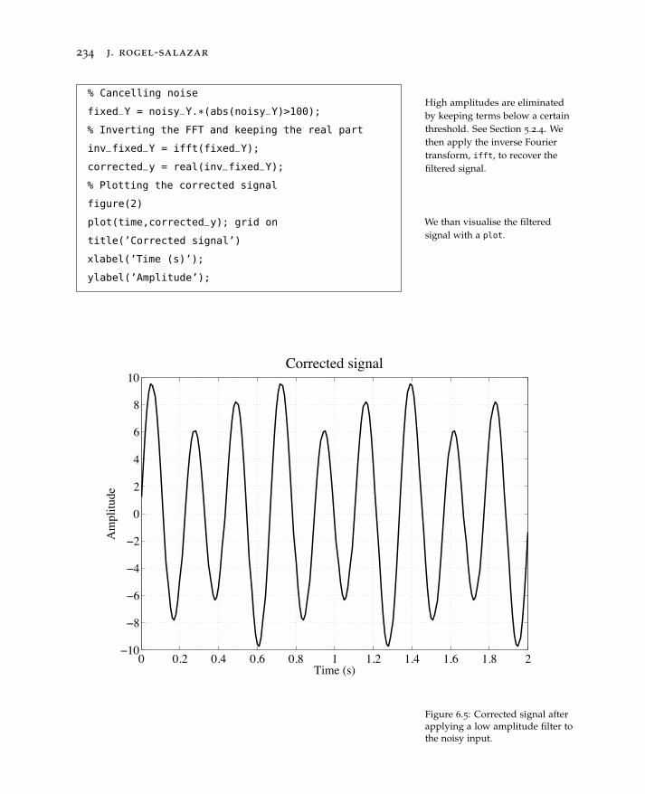
234 j. rogel-salazar

% Cancelling noise

fixed_Y = noisy_Y.*(abs(noisy_Y)>100);

% Inverting the FFT and keeping the real part

inv_fixed_Y = ifft(fixed_Y);

corrected_y = real(inv_fixed_Y);

% Plotting the corrected signal

figure(2)

plot(time,corrected_y); grid on

title(’Corrected signal’)

xlabel(’Time (s)’);

ylabel(’Amplitude’);

High amplitudes are eliminatedby keeping terms below a certainthreshold. See Section 5.2.4. Wethen apply the inverse Fouriertransform, ifft, to recover thefiltered signal.

We than visualise the filteredsignal with a plot.

0 0.2 0.4 0.6 0.8 1 1.2 1.4 1.6 1.8 2ï10

ï8

ï6

ï4

ï2

0

2

4

6

8

10Corrected signal

Time (s)

Am

plitu

de

Figure 6.5: Corrected signal afterapplying a low amplitude filter tothe noisy input.

essential matlab®

and octave 235

As we can see from Figure 6.5 the filtering has worked quite

well and thus we have recovered a fairly good match for our

original signal.

6.6 Physics: The Wave Equation

The wave equation provides a straightforward way to

model the propagation of waves of different kinds: light,

sound, oscillating strings and membranes, etc. The wave

equation in one dimension is given by the following partial

differential equation7: 7 Elmore, W. and M. Heald (2012).Physics of Waves. Dover Books onPhysics. Dover Publications∂2E

∂t2 − c2 ∂2E∂x2 = 0, (6.49)

where E = E(x, t) is a function that gives the amplitude

of the wave at time t in position x, and c is the speed with

which the wave propagates.

6.6.1 Oscillations in a String

We are interested in modelling the oscillations of

a string, for instance in a guitar. Let us consider that the We model the oscillations in aguitar string for example.length of the string is 10 cm and that the wave propagates

at a speed of 5 cm/s. Both ends of the string are fixed at a

height x = 0.

We tackle the solution of the wave Equation (6.49) using

finite differences. Let us recall that the second derivative

of a function can be approximated with the use of central

differences as:

Finite difference approximation forthe second derivative.f ′′(x) ' 1

∆x2 ( f (x + ∆x)− 2 f (x) + f (x− ∆x)) . (6.50)

236 j. rogel-salazar

0 1 2 3 4 5 6 7 8 9 10ï2

ï1.5

ï1

ï0.5

0

0.5

1

1.5

2Oscillating string

x (cm)

Hei

ght,

E(x,

t)

Figure 6.6: Initial condition for thesimulation of an oscillating string.

This means that we can express Equation (6.49) as

1∆t2 (E(x, t + ∆t)− 2E(x, t) + f (x, t− ∆t)) =

c2

∆x2 (E(x + ∆x, t)− 2E(x, t) + E(x− ∆x, t)) . (6.51)

This expression depends on earlier,current and future times.

Notice that we have three different times in play here: the

time now (t), later times (t + ∆t) and earlier times (t −∆t). We can use this to our advantage such that we can

predict the position at later times based on current and past

positions.

essential matlab®

and octave 237

We use the expression above to solve for later times, i.e.

t + ∆t:

E(x, t + ∆t) = r2 (E(x + ∆x, t) + E(x − ∆x, t)) +

2(1 − r2)E(x, t) − E(x, t − ∆t), (6.52)

We have expressed the position atlater times in terms of current andpast positions.

where r = c∆t∆x . If we choose ∆t to be small enough such

that r < 12 , then the numerical solution will be stable;

otherwise we end up with ever larger waves. We shall

consider the initial condition

We need to provide an initialcondition for the simulation.

E(x, 0) =12

(1 − cos

(2πx

L

)), (6.53)

as shown in Figure 6.6.

The script StringOscillation.m implements the simulation.

We shall divide the script into two parts. First, let us set up

the parameters of the simulation as follows:

We define the values for ∆xand ∆t, as well as the values forparameters such as L, c and theduration of the simulation.

This enables us to define thediscretisation of the length ofthe string and set up the initialcondition.

% Script StringOscillation.m

% Defining parameters

delta_x = 0.01;

delta_t = 0.001;

c = 5;

L = 10;

end_sim=30;

r=c*delta_t/delta_x;

n = L/delta_x +1;

string = [0:delta_x:L];

% Setting initial condition to a cos function

now_t = (1/2)*(1-cos(2*pi/L*string));

earlier_t=now_t;

238 j. rogel-salazar

We implement the finite difference update outlined in

Equation (6.52). The result of the script below results in an

animated plot, and thus we recommend trying the script to

see the end result.

This script will result in ananimation.

We implement the finite differencescheme, fixing the end points ofthe string.

On each iteration we update thetime (see Section 5.3). Finally, wegenerate a plot.

% Wave equation solution

for time=0:delta_t:end_sim

% calculate future position

later_t(1)=0;

later_t(2:n-1)=r^2*(now_t(1:n-2)+...

now_t(3:n)) + ...

2*(1-r^2)*now_t(2:n-1) - earlier_t(2:n-1);

later_t(n) = 0;

% update status for next iteration

earlier_t = now_t;

now_t = later_t;

% plot the status every 20th frame

if mod(time/delta_t, 20)==0

plot(string,now_t);

title(’Oscillating string’);

xlabel(’x (cm)’);

ylabel(’Height, E(x,t)’);

axis([0 L -2 2])

pause(0.001)

end

end

6.6.2 Oscillations in a Circular Membrane

In the previous section we have seen how the oscilla-

tions in a string can be modelled with the aid of MATLAB

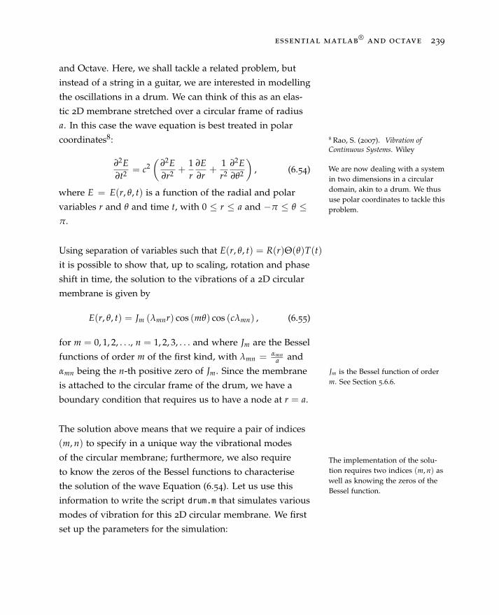
essential matlab®

and octave 239

and Octave. Here, we shall tackle a related problem, but

instead of a string in a guitar, we are interested in modelling

the oscillations in a drum. We can think of this as an elas-

tic 2D membrane stretched over a circular frame of radius

a. In this case the wave equation is best treated in polar

coordinates8: 8 Rao, S. (2007). Vibration ofContinuous Systems. Wiley

∂2E∂t2 = c2

(∂2E∂r2 +

1r

∂E∂r

+1r2

∂2E∂θ2

), (6.54)

where E = E(r, θ, t) is a function of the radial and polar

variables r and θ and time t, with 0 ≤ r ≤ a and −π ≤ θ ≤π.

We are now dealing with a systemin two dimensions in a circulardomain, akin to a drum. We thususe polar coordinates to tackle thisproblem.

Using separation of variables such that E(r, θ, t) = R(r)Θ(θ)T(t)it is possible to show that, up to scaling, rotation and phase

shift in time, the solution to the vibrations of a 2D circular

membrane is given by

E(r, θ, t) = Jm (λmnr) cos (mθ) cos (cλmn) , (6.55)

for m = 0, 1, 2, . . ., n = 1, 2, 3, . . . and where Jm are the Bessel

functions of order m of the first kind, with λmn = αmna and

αmn being the n-th positive zero of Jm. Since the membrane Jm is the Bessel function of orderm. See Section 5.6.6.is attached to the circular frame of the drum, we have a

boundary condition that requires us to have a node at r = a.

The solution above means that we require a pair of indices

(m, n) to specify in a unique way the vibrational modes

of the circular membrane; furthermore, we also require

to know the zeros of the Bessel functions to characterise

the solution of the wave Equation (6.54). Let us use this

The implementation of the solu-tion requires two indices (m, n) aswell as knowing the zeros of theBessel function.

information to write the script drum.m that simulates various

modes of vibration for this 2D circular membrane. We first

set up the parameters for the simulation:

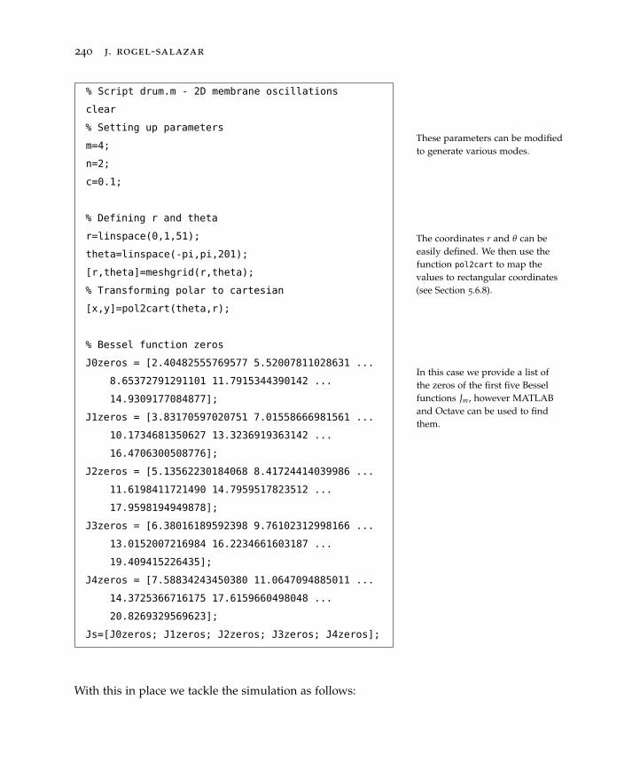
240 j. rogel-salazar

% Script drum.m - 2D membrane oscillations

clear

% Setting up parameters

m=4;

n=2;

c=0.1;

% Defining r and theta

r=linspace(0,1,51);

theta=linspace(-pi,pi,201);

[r,theta]=meshgrid(r,theta);

% Transforming polar to cartesian

[x,y]=pol2cart(theta,r);

% Bessel function zeros

J0zeros = [2.40482555769577 5.52007811028631 ...

8.65372791291101 11.7915344390142 ...

14.9309177084877];

J1zeros = [3.83170597020751 7.01558666981561 ...

10.1734681350627 13.3236919363142 ...

16.4706300508776];

J2zeros = [5.13562230184068 8.41724414039986 ...

11.6198411721490 14.7959517823512 ...

17.9598194949878];

J3zeros = [6.38016189592398 9.76102312998166 ...

13.0152007216984 16.2234661603187 ...

19.409415226435];

J4zeros = [7.58834243450380 11.0647094885011 ...

14.3725366716175 17.6159660498048 ...

20.8269329569623];

Js=[J0zeros; J1zeros; J2zeros; J3zeros; J4zeros];

These parameters can be modifiedto generate various modes.

The coordinates r and θ can beeasily defined. We then use thefunction pol2cart to map thevalues to rectangular coordinates(see Section 5.6.8).

In this case we provide a list ofthe zeros of the first five Besselfunctions Jm, however MATLABand Octave can be used to findthem.

With this in place we tackle the simulation as follows:

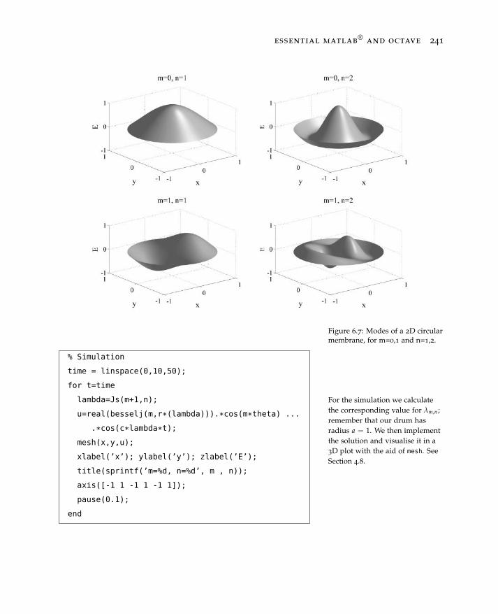
essential matlab®

and octave 241

Figure 6.7: Modes of a 2D circularmembrane, for m=0,1 and n=1,2.

% Simulation

time = linspace(0,10,50);

for t=time

lambda=Js(m+1,n);

u=real(besselj(m,r*(lambda))).*cos(m*theta) ...

.*cos(c*lambda*t);

mesh(x,y,u);

xlabel(’x’); ylabel(’y’); zlabel(’E’);

title(sprintf(’m=%d, n=%d’, m , n));

axis([-1 1 -1 1 -1 1]);

pause(0.1);

end

For the simulation we calculatethe corresponding value for λm,n;remember that our drum hasradius a = 1. We then implementthe solution and visualise it in a3D plot with the aid of mesh. SeeSection 4.8.

242 j. rogel-salazar

The result of the simulation above is a series of frames in

the same figure, providing a rudimentary animation. We

recommend trying the code above in your own computer to

see the modes in action. To give us an idea of what we shall

see, we have plotted some of the vibrational modes for the

2D circular membrane in Figure 6.7 .

We will end up with an animatedplot. We recommend trying thisout to see the result.

6.7 Quantum Mechanics: The Schrödinger Equation andPauli Matrices

The use of matrices in quantum mechanics is prominent:

they are employed to represent physical quantities, describ-

ing states on a quantum system. This approach requires the

constant use of linear algebra and what better tools than

MATLAB and Octave to do so.

Linear algebra lies at the heartof quantum mechanics. UsingMATLAB and Octave can facilitatesome relevant operations.

6.7.1 Particle in an Infinite Potential Well

One of the simplest systems in quantum mechanics is a

particle confined in an infinite potential well. In this case we

are interested in describing the discrete energy levels using

the time-independent Schrödinger equation9. 9 Griffiths, D. (2005). Introductionto Quantum Mechanics. PearsonEducationLet us consider a quantum mechanical particle with wave-

function ψ(x) in one dimension. The particle is confined

to a square well with impenetrable walls in the region

0 < x < L. This means that we have boundary conditions

that require the wavefunction to vanish at both ends, i.e.

x = 0 and x = L. We therefore expect to end up with stable

standing waves inside the box.

The wavefunctions for the statesin a one-dimensional box arestanding waves.

The time-independent Schödinger equation is given by

The Schrödinger equation is aneigenvalue problem.

Hψ(x) = Eψ(x), (6.56)

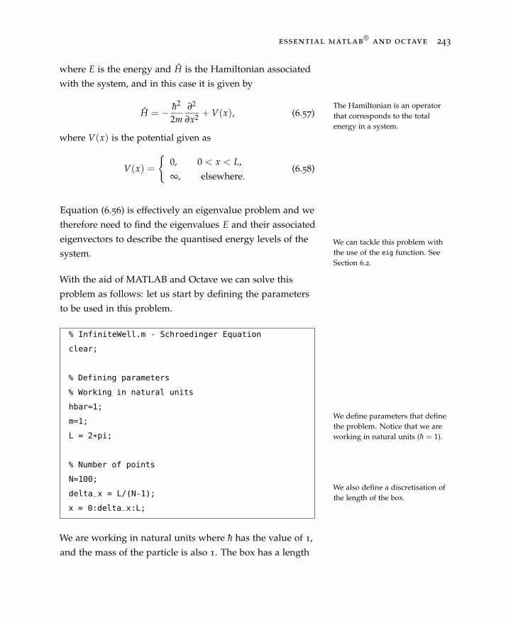
essential matlab®

and octave 243

where E is the energy and H is the Hamiltonian associated

with the system, and in this case it is given by

The Hamiltonian is an operatorthat corresponds to the totalenergy in a system.

H = − h2

2m∂2

∂x2 + V(x), (6.57)

where V(x) is the potential given as

V(x) =

{0, 0 < x < L,

∞, elsewhere.(6.58)

Equation (6.56) is effectively an eigenvalue problem and we

therefore need to find the eigenvalues E and their associated

eigenvectors to describe the quantised energy levels of the

system.

With the aid of MATLAB and Octave we can solve this

problem as follows: let us start by defining the parameters

to be used in this problem.

We can tackle this problem withthe use of the eig function. SeeSection 6.2.

We define parameters that definethe problem. Notice that we areworking in natural units (h = 1).

We also define a discretisation ofthe length of the box.

% InfiniteWell.m - Schroedinger Equation

clear;

% Defining parameters

% Working in natural units

hbar=1;

m=1;

L = 2*pi;

% Number of points

N=100;

delta_x = L/(N-1);

x = 0:delta_x:L;

We are working in natural units where h has the value of 1,

and the mass of the particle is also 1. The box has a length

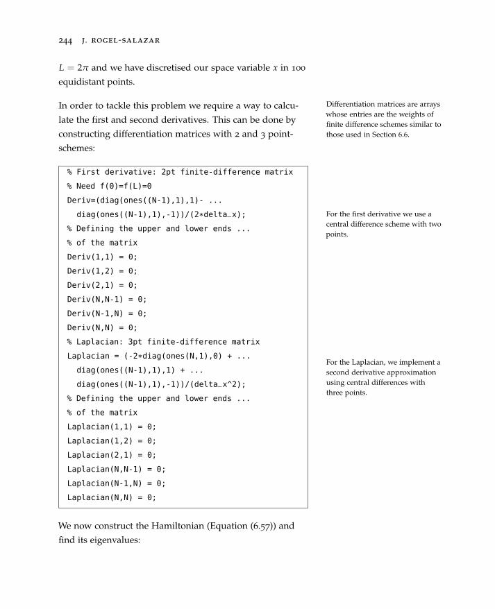
244 j. rogel-salazar

L = 2π and we have discretised our space variable x in 100

equidistant points.

In order to tackle this problem we require a way to calcu-

late the first and second derivatives. This can be done by

constructing differentiation matrices with 2 and 3 point-

schemes:

Differentiation matrices are arrayswhose entries are the weights offinite difference schemes similar tothose used in Section 6.6.

For the first derivative we use acentral difference scheme with twopoints.

For the Laplacian, we implement asecond derivative approximationusing central differences withthree points.

% First derivative: 2pt finite-difference matrix

% Need f(0)=f(L)=0

Deriv=(diag(ones((N-1),1),1)- ...

diag(ones((N-1),1),-1))/(2*delta_x);

% Defining the upper and lower ends ...

% of the matrix

Deriv(1,1) = 0;

Deriv(1,2) = 0;

Deriv(2,1) = 0;

Deriv(N,N-1) = 0;

Deriv(N-1,N) = 0;

Deriv(N,N) = 0;

% Laplacian: 3pt finite-difference matrix

Laplacian = (-2*diag(ones(N,1),0) + ...

diag(ones((N-1),1),1) + ...

diag(ones((N-1),1),-1))/(delta_x^2);

% Defining the upper and lower ends ...

% of the matrix

Laplacian(1,1) = 0;

Laplacian(1,2) = 0;

Laplacian(2,1) = 0;

Laplacian(N,N-1) = 0;

Laplacian(N-1,N) = 0;

Laplacian(N,N) = 0;

We now construct the Hamiltonian (Equation (6.57)) and

find its eigenvalues:

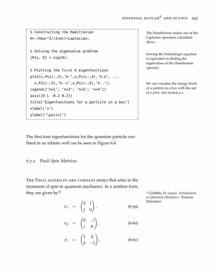
essential matlab®

and octave 245

% Constructing the Hamiltonian

H=-(hbar^2/(2*m))*Laplacian;

% Solving the eigenvalue problem

[Psi, E] = eig(H);

% Plotting the first 4 eigenfunctions

plot(x,Psi(:,3),’k-’,x,Psi(:,4),’k:o’, ...

x,Psi(:,5),’k--+’,x,Psi(:,6),’k-.’);

legend([’n=1’; ’n=2’; ’n=3’; ’n=4’])

axis([0 L -0.2 0.2])

title(’Eigenfunctions for a particle in a box’)

xlabel(’x’)

ylabel(’\psi(x)’)

The Hamiltonian makes use of theLaplacian operation calculatedabove.

Solving the Schrödinger equationis equivalent to finding theeigenvalues of the Hamiltonianoperator.

We can visualise the energy levelsof a particle in a box with the aidof a plot. See Section 4.1.

The first four eigenfunctions for the quantum particle con-

fined in an infinite well can be seen in Figure 6.8.

6.7.2 Pauli Spin Matrices

The Pauli matrices are complex arrays that arise in the

treatment of spin in quantum mechanics. In a unitless form

they are given by10 10 Griffiths, D. (2005). Introductionto Quantum Mechanics. PearsonEducation

σx =

(0 1

1 0

), (6.59)

σy =

(0 −ii 0

), (6.60)

σz =

(1 0

0 −1

). (6.61)

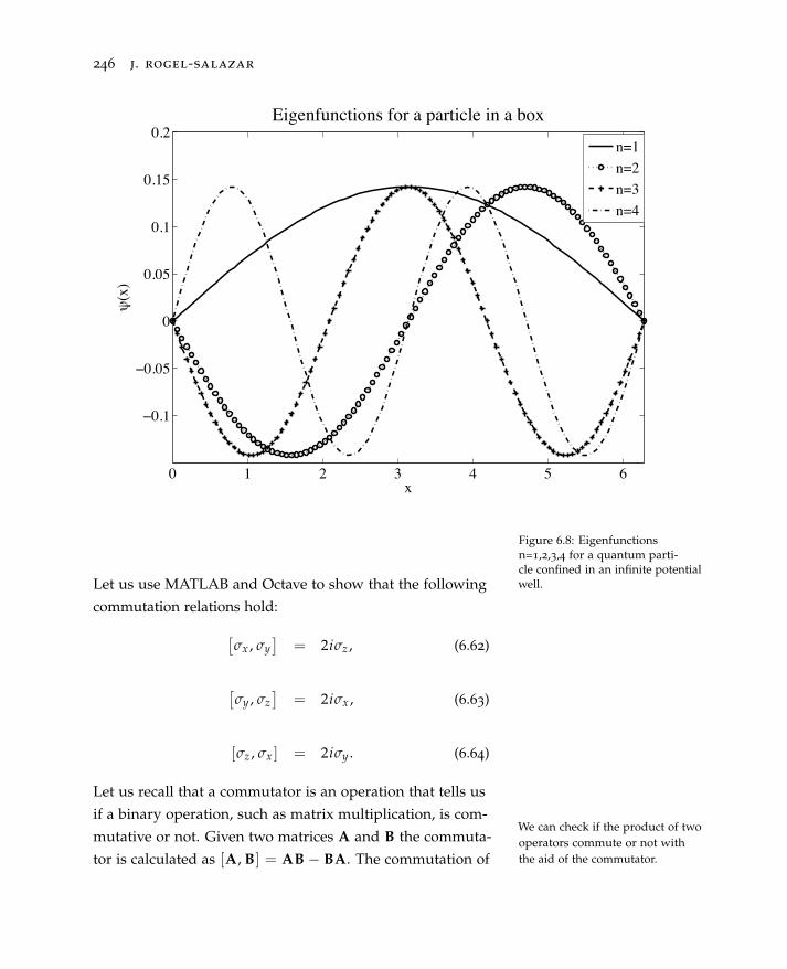
246 j. rogel-salazar

0 1 2 3 4 5 6

ï0.1

ï0.05

0

0.05

0.1

0.15

0.2

x

s(x

)Eigenfunctions for a particle in a box

n=1n=2n=3n=4

Figure 6.8: Eigenfunctionsn=1,2,3,4 for a quantum parti-cle confined in an infinite potentialwell.Let us use MATLAB and Octave to show that the following

commutation relations hold:[σx , σy

]= 2iσz , (6.62)

[σy , σz

]= 2iσx , (6.63)

[σz , σx ] = 2iσy . (6.64)

Let us recall that a commutator is an operation that tells us

if a binary operation, such as matrix multiplication, is com-

mutative or not. Given two matrices A and B the commuta-

tor is calculated as [A, B] = AB − BA. The commutation of

We can check if the product of twooperators commute or not withthe aid of the commutator.

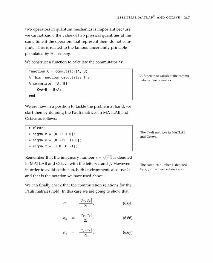
essential matlab®

and octave 247

two operators in quantum mechanics is important because

we cannot know the value of two physical quantities at the

same time if the operators that represent them do not com-

mute. This is related to the famous uncertainty principle

postulated by Heisenberg.

We construct a function to calculate the commutator as:

A function to calculate the commu-tator of two operators.

function C = commutator(A, B)

% This function calculates the

% commutator [A, B]

C=A*B - B*A;

end

We are now in a position to tackle the problem at hand; we

start then by defining the Pauli matrices in MATLAB and

Octave as follows:

The Pauli matrices in MATLABand Octave.

> clear;

> sigma_x = [0 1; 1 0];

> sigma_y = [0 -1i; 1i 0];

> sigma_z = [1 0; 0 -1];

Remember that the imaginary number i =√−1 is denoted

in MATLAB and Octave with the letters i and j. However,

in order to avoid confusion, both environments also use 1i

and that is the notation we have used above.

The complex number is denotedby i, j or 1i. See Section 1.5.1.

We can finally check that the commutation relations for the

Pauli matrices hold. In this case we are going to show that

σz =[σx , σy ]

2i, (6.65)

σx =[σy , σz ]

2i, (6.66)

σy =[σz , σx ]

2i. (6.67)

248 j. rogel-salazar

> R1 = commutator(sigma_x,sigma_y)/(2*1i)

R1 =

1 0

0 -1

> R2 = commutator(sigma_y,sigma_z)/(2*1i)

R2 =

0 1

1 0

> R3 = commutator(sigma_z,sigma_x)/(2*1i)

R3 =

0.0000 + 0.0000i 0.0000 - 1.0000i

0.0000 + 1.0000i 0.0000 + 0.0000i

We can see that by dividing the result of each commutator

The result of the commutatordivided by 2i indeed returns thethird Pauli matrix.

between two Pauli matrices (in correct cyclical order) by 2iwe recover the third one.

6.8 Summary

As we have seen in this chapter, the flexibility and versa-

tility offered by MATLAB and Octave make them suitable to

tackle a wide range of problems and subjects.

In this case we have chosen a small number of topics with

a few examples. Our main objective here has been to show

how the different elements of the software are combined

together to address a particular set of tasks within the

essential matlab®

and octave 249

context of particular applications. An in-depth discussion of

these topics goes beyond the scope of this book.

We have seen how MATLAB and Octave can successfully

be used for calculations directly involving linear algebra;

matrices are, after all, the main element of the software.

Optimisation problems are typical of a number of appli-

cations and in this case we have chosen to use portfolio

management to exemplify the implementation of a very ba-

sic optimisation technique: Lagrange multipliers. Similarly,

another important tool used in various areas is the numer-

ical solution of differential equations; here we have used a

predator-prey model to demonstrate the way to solve a sys-

tem of ordinary differential equations. In the case of partial

differential equations, we have used the wave equation as

a way to show an implementation of finite differences to

tackle this sort of problem.

Other applications included here are signal processing and

noise filtering, the simulation of the oscillations in a circular

membrane, as well as the solution of the time-independent

Schrödinger equation for an infinite potential well and

simple manipulations of spin matrices. We very much hope

that these examples enable you, the reader, to use MATLAB

and Octave in your own problem-solving tasks.

250 j. rogel-salazar

6.9 Exercises

The following exercises are related to the subjects discussed

in this chapter. In order to tackle the exercises you are

expected to be familiar with the topics and we recommend

taking a look at the references used in this chapter for

further details.

1. The angle θ between two vectors u and v can be obtained

by recalling that the dot product of the two vectors can be

expressed as

u · v = |u||v| cos θ .

Write a function that takes any two vectors, checks if they

have the same length and calculates the angle θ between

them.

2. Write a function that takes a vector v, and returns a unit

vector v. Your functions should check for zero-norm

vectors.

3. Find out what the functions rank and rref do. Write

a function that takes a general linear system of linear

equations Ax = b with m equations and n variables.

Determine whether the system has a unique solution

and find the answer. Otherwise if the rank of the matrix

A is different from the number of variables, display the

augmented matrix using the rref function.

4. The Gram-Schmidt process is a procedure that builds

an orthonormal basis over an arbitrary interval out of a

given nonorthogonal set of linearly independent func-

tions11. With the aid of an appropriate reference such 11 Strang, G. (2003). Introductionto Linear Algebra. Wellesley-Cambridge Pressas the one suggested, write an m-function that imple-

ments the Gram-Schmidt algorithm for n independent

vectors a1, a2, . . . , an to produce n orthonormal vectors

q1, q2, . . . , qn.

essential matlab®

and octave 251

5. Consider the two three-asset portfolios used in Section

6.3 such that the weights of the minimum variance port-

folio are given by the vector wa. Similarly, wb are the

weights of the portfolio with target return µb = 0.1. For

a situation where short-selling is allowed, write a script

that calculates and plots the efficient frontier using a

convex combination of portfolios wa and wb.

6. Use MATLAB and Octave to solve and plot the solution

to the following second-order differential equation:

y′′(c)+ 8y′(x)+ 2y(x) = cos(x); y(0) = 0, y′(0) = 1.

Hint: Rewrite the equation as a first-order system.

7. Consider the Lorenz equations:

dxdt

= −55(x + y),

dydt

= −y− 5xz,

dzdt

= xy− 4z− 420,

with the following initial conditions: x(0) = −5, y(0) = 5

and z(0) = 15. Solve the system of differential equations

using MATLAB and Octave for a time interval [0, 8].

Finally, produce a plot of z(t) versus x(t).

8. Consider the following signal:

y = 2 sin(6πt) + 8 sin(9πt).

Add some noise to it in the form of a sine wave of am-

plitude 5 and frequency 60 Hz. Plot the original and the

noisy signals, as well as their amplitude spectra. Finally,

use the Fourier transform to remove the high frequency

noise and compare the results to the original signal.

252 j. rogel-salazar

9. Consider the diffusion equation:

∂U∂t

= α∂2U∂x2 ,

which can be used to model the temperature diffusion

in a slab of length L = 1 with diffusivity α = 1 × 10−2.

Write a script to model the temperature diffusion in the

slab for an initial condition given by

U(x, 0) = sin(

2πxL

),

and subject to the boundary conditions U(0, t) = 0 and

U(L, t) = 0.

10. Using the Pauli spin matrices we can represent the spin

state of a spin- 12 particle by a two-element column vector.

For spin up and down these vectors are, respectively,

given by

|↑〉 =(

1

0

), |↓〉 =

(0

1

).

(a) Verify that operating on these vectors from the left

with the matrix σz yields + |↑〉 and − |↓〉, respectively.

(b) Construct a column vector |→〉 with the property

that σx |→〉 = + |→〉, which corresponds to a spin- 12

particle with spin in the + x direction.

(c) Finally, construct a column vector |⊗〉 with the prop-

erty that σy |⊗〉 = + |⊗〉, which corresponds to a

spin- 12 particle with spin in the +y direction.

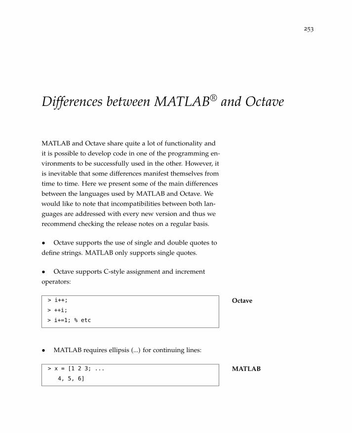
253

Differences between MATLAB® and Octave

MATLAB and Octave share quite a lot of functionality and

it is possible to develop code in one of the programming en-

vironments to be successfully used in the other. However, it

is inevitable that some differences manifest themselves from

time to time. Here we present some of the main differences

between the languages used by MATLAB and Octave. We

would like to note that incompatibilities between both lan-

guages are addressed with every new version and thus we

recommend checking the release notes on a regular basis.

• Octave supports the use of single and double quotes to

define strings. MATLAB only supports single quotes.

• Octave supports C-style assignment and increment

operators:

Octave> i++;

> ++i;

> i+=1; % etc

• MATLAB requires ellipsis (...) for continuing lines:

MATLAB> x = [1 2 3; ...

4, 5, 6]

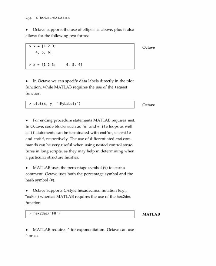
254 j. rogel-salazar

• Octave supports the use of ellipsis as above, plus it also

allows for the following two forms:

Octave> x = [1 2 3;

4, 5, 6]

> x = [1 2 3; 4, 5, 6]

• In Octave we can specify data labels directly in the plot

function, while MATLAB requires the use of the legend

function.

Octave> plot(x, y, ’;MyLabel;’)

• For ending procedure statements MATLAB requires end.

In Octave, code blocks such as for and while loops as well

as if statements can be terminated with endfor, endwhile

and endif, respectively. The use of differentiated end com-

mands can be very useful when using nested control struc-

tures in long scripts, as they may help in determining when

a particular structure finishes.

• MATLAB uses the percentage symbol (%) to start a

comment. Octave uses both the percentage symbol and the

hash symbol (#).

• Octave supports C-style hexadecimal notation (e.g.,

“0xF0”) whereas MATLAB requires the use of the hex2dec

function:

MATLAB> hex2dec(’F0’)

• MATLAB requires ^ for exponentiation. Octave can use

^ or **.

essential matlab®

and octave 255

• The debugger that comes embedded in MATLAB has

more advanced features such as graphical stops and contin-

uation commands.

• MATLAB has a number of toolboxes that can be ac-

quired separately from The MathWorks. Some implementa-

tions of similar capabilities are available for Octave. How-

ever some may not be as complete or may not be available.

• MATLAB is capable of producing Graphical User Inter-

faces (GUIs) with the help of guide. This capability is not

available in Octave.

257

Bibliography

Britton, N. (2003). Essential Mathematical Biology. Springer

Undergraduate Mathematics Series. Springer London.

Eaton, J. W., D. Bateman, and S. Hauberg (2008). GNUOctave Manual: Version 3. A GNU manual. Network Theory

Limited.

Elmore, W. and M. Heald (2012). Physics of Waves. Dover

Books on Physics. Dover Publications.

Elton, E., M. Gruber, S. Brown, and W. Goetzmann (2009).

Modern Portfolio Theory and Investment Analysis. John Wiley

& Sons.

GNU (June 29, 2007). General Public License, Free Software

Foundation, version 3. http://www.gnu.org/licenses/gpl

(Last visited Aug 4,2014).

Griffiths, D. (2005). Introduction to Quantum Mechanics.

Pearson Education.

Hansen, J. S. (2011). GNU Octave Beginner’s Guide. Learn by

doing: less theory, more results. Packt Publishing, Limited.

Higham, D. J. and N. J. Higham (2005). MATLAB Guide.

Society for Industrial and Applied Mathematics.

Palm, W. J. (2008). A Concise Introduction to MATLAB.

McGraw-Hill Higher Education.

258 j. rogel-salazar

Priemer, R. (1991). Introductory Signal Processing. Advanced

Series in Electrical and Computer Engineering. World

Scientific.

Rao, S. (2007). Vibration of Continuous Systems. Wiley.

Strang, G. (2003). Introduction to Linear Algebra. Wellesley-

Cambridge Press.

ESSENTIAL M

ATLAB®AN

D OCTAVERogel-Salazar

ISBN: 978-1-4822-3463-3

9 781482 234633

90000

K23005

Mathematics

“Essential MATLAB® and Octave is a superb introductory textbook for those interested in learning how to solve scientific, engineering, and mathematical problems using two of the most popular mathematical programming tools available. The book assumes almost no prior experience with programming or scientific programming, and carefully takes the reader step by step through the use of the two languages for solving increasingly complex problems. …Dr. Rogel-Salazar has put a huge amount of effort into making the book accessible and user friendly in a way that makes it suitable even for the most novices of programmers.” —Dr. Shashank Virmani, Brunel University London, UK

“The text provides a clear and easy-paced introduction to MATLAB® and Octave. The presentation is example led and contains plenty of useful applications drawn from mathematics, physics, and engineering. This beginner’s handbook will suit a broad scientific readership.” —Dr. Alan McCall, University of Hertfordshire, UK

Learn Two Popular Programming Languages in a Single Volume

Widely used by scientists and engineers, well-established MATLAB® and open-source Octave are similar software programs providing excellent capabilities for data analysis, visualization, and more. By means of straightforward explanations and examples from different areas in mathematics, engineering, finance, and physics, Essential MATLAB and Octave explains how MATLAB and Octave are powerful tools applicable to a variety of problems. This text provides an introduction that reveals basic structures and syntax, demonstrates the use of functions and procedures, outlines availability in various platforms, and highlights the most important elements for both programs.

Effectively Implement Models and Prototypes Using Computational Models

This text requires no prior knowledge. Self-contained, it allows the reader to use the material whenever needed rather than follow a particular order. Compatible with both languages, the book material incorporates commands and structures that allow the reader to gain a greater awareness of MATLAB and Octave, write their own code, and implement their scripts and programs within a variety of applicable fields. It is always made clear when particular examples apply only to MATLAB or only to Octave, allowing the book to be used flexibly depending on readers’ requirements.

Essential MATLAB and Octave offers an introductory course in MATLAB and Octave programming, and is a perfect resource for students in physics, mathematics, statistics, engineering, and any other subjects that require the use of computers to solve numerical problems.

K23005_COVER_final.indd 1 9/26/14 10:44 AM