polynomial computations in matlab · pdf fileabstract this report details how the following...
TRANSCRIPT

Polynomial Computations in MATLAB1
Kannan M. Moudgalya
Dept. of Chemical Engineering and
Systems and Control Group
Indian Institute of Technology
Powai, Mumbai 400 076
India
November 1996
1Supported by the Department of Science and Technology through Grant No. III.5(11)/91-ET

Abstract
This report details how the following polynomial matrix computations have been im-
plemented in MATLAB: coprime factorization, solutions to Aryabhatta’s Identity and
unilateral and bilateral polynomial equations. A complete listing of the source code is
provided. Usage of the software is illustrated with several examples.

Contents
1 Introduction 1
2 Left coprime factorization 3
2.1 Algorithm (Chang and Pearson, 1982) . . . . . . . . . . . . . . . . . . . 3
2.2 Conventions . . . . . . . . . . . . . . . . . . . . . . . . . . . . . . . . . . 4
2.3 Example: Coprime factorization . . . . . . . . . . . . . . . . . . . . . . . 5
2.3.1 Input program listing (data01.m) . . . . . . . . . . . . . . . . . . 5
2.3.2 Output from MATLAB . . . . . . . . . . . . . . . . . . . . . . . . 6
2.3.3 Result . . . . . . . . . . . . . . . . . . . . . . . . . . . . . . . . . 6
2.4 Example: Checking whether a given polynomial matrix is unimodular . . 7
2.4.1 Input program listing . . . . . . . . . . . . . . . . . . . . . . . . . 7
2.4.2 Output from MATLAB . . . . . . . . . . . . . . . . . . . . . . . . 7
2.5 Example: Producing a row proper polynomial . . . . . . . . . . . . . . . 8
2.5.1 Input program listing . . . . . . . . . . . . . . . . . . . . . . . . . 8
2.5.2 Output from MATLAB . . . . . . . . . . . . . . . . . . . . . . . . 8
2.6 Programs . . . . . . . . . . . . . . . . . . . . . . . . . . . . . . . . . . . 9
3 Aryabhatta’s Identity 10
3.1 Algorithm (Chang and Pearson, 1982) . . . . . . . . . . . . . . . . . . . 10
3.2 Usage . . . . . . . . . . . . . . . . . . . . . . . . . . . . . . . . . . . . . 10
3.2.1 Input program listing (data04.m) . . . . . . . . . . . . . . . . . . 10
3.2.2 Output from MATLAB (ex04.out) . . . . . . . . . . . . . . . . . 11
3.2.3 Result . . . . . . . . . . . . . . . . . . . . . . . . . . . . . . . . . 12
3.3 Programs . . . . . . . . . . . . . . . . . . . . . . . . . . . . . . . . . . . 12
4 Unilateral polynomial matrix equation 12
4.1 Algorithm (Chang and Pearson, 1982) . . . . . . . . . . . . . . . . . . . 12
4.2 Usage . . . . . . . . . . . . . . . . . . . . . . . . . . . . . . . . . . . . . 13
4.2.1 First example . . . . . . . . . . . . . . . . . . . . . . . . . . . . . 13
4.2.2 Second example . . . . . . . . . . . . . . . . . . . . . . . . . . . . 14
4.3 Programs . . . . . . . . . . . . . . . . . . . . . . . . . . . . . . . . . . . 15
5 Generalized Aryabhatta’s Identity 16
5.1 Algorithm (Chang and Pearson, 1982) . . . . . . . . . . . . . . . . . . . 16
5.1.1 Step1: Find A(s) and B(s) . . . . . . . . . . . . . . . . . . . . . . 16
5.1.2 Step2: Find A1(s), B1(s), X(s) and Y (s) . . . . . . . . . . . . . . 16
5.1.3 Step 3: Find X1(s) and Y1(s) . . . . . . . . . . . . . . . . . . . . 17
5.2 Usage . . . . . . . . . . . . . . . . . . . . . . . . . . . . . . . . . . . . . 17
i

5.2.1 First example . . . . . . . . . . . . . . . . . . . . . . . . . . . . . 17
5.2.2 Second example . . . . . . . . . . . . . . . . . . . . . . . . . . . . 19
5.3 Programs . . . . . . . . . . . . . . . . . . . . . . . . . . . . . . . . . . . 22
6 Bilateral polynomial matrix equation 22
6.1 Algorithm (Chang and Pearson, 1982) . . . . . . . . . . . . . . . . . . . 23
6.2 Usage . . . . . . . . . . . . . . . . . . . . . . . . . . . . . . . . . . . . . 23
6.2.1 First example . . . . . . . . . . . . . . . . . . . . . . . . . . . . . 23
6.2.2 Second example . . . . . . . . . . . . . . . . . . . . . . . . . . . . 24
6.3 Programs . . . . . . . . . . . . . . . . . . . . . . . . . . . . . . . . . . . 26
7 Numerical issues 26
7.1 Linear dependence . . . . . . . . . . . . . . . . . . . . . . . . . . . . . . 27
7.2 Zeroing small entries . . . . . . . . . . . . . . . . . . . . . . . . . . . . . 27
A MATLAB routines 28
A.1 arya.m . . . . . . . . . . . . . . . . . . . . . . . . . . . . . . . . . . . . . 28
A.1.1 Purpose . . . . . . . . . . . . . . . . . . . . . . . . . . . . . . . . 28
A.1.2 mfiles called . . . . . . . . . . . . . . . . . . . . . . . . . . . . . . 28
A.1.3 Listing of the code . . . . . . . . . . . . . . . . . . . . . . . . . . 28
A.2 cindep.m . . . . . . . . . . . . . . . . . . . . . . . . . . . . . . . . . . . . 29
A.2.1 Purpose . . . . . . . . . . . . . . . . . . . . . . . . . . . . . . . . 29
A.2.2 mfiles called . . . . . . . . . . . . . . . . . . . . . . . . . . . . . . 29
A.2.3 Listing of the code . . . . . . . . . . . . . . . . . . . . . . . . . . 29
A.3 clcoef.m . . . . . . . . . . . . . . . . . . . . . . . . . . . . . . . . . . . . 30
A.3.1 Purpose . . . . . . . . . . . . . . . . . . . . . . . . . . . . . . . . 30
A.3.2 mfiles called . . . . . . . . . . . . . . . . . . . . . . . . . . . . . . 30
A.3.3 Listing of the code . . . . . . . . . . . . . . . . . . . . . . . . . . 30
A.4 flat2nor.m . . . . . . . . . . . . . . . . . . . . . . . . . . . . . . . . . . . 31
A.4.1 Purpose . . . . . . . . . . . . . . . . . . . . . . . . . . . . . . . . 31
A.4.2 mfiles called . . . . . . . . . . . . . . . . . . . . . . . . . . . . . . 31
A.4.3 Listing of the code . . . . . . . . . . . . . . . . . . . . . . . . . . 31
A.5 indep.m . . . . . . . . . . . . . . . . . . . . . . . . . . . . . . . . . . . . 32
A.5.1 Purpose . . . . . . . . . . . . . . . . . . . . . . . . . . . . . . . . 32
A.5.2 mfiles called . . . . . . . . . . . . . . . . . . . . . . . . . . . . . . 32
A.5.3 Listing of the code . . . . . . . . . . . . . . . . . . . . . . . . . . 32
A.6 issoln.m . . . . . . . . . . . . . . . . . . . . . . . . . . . . . . . . . . . . 33
A.6.1 Purpose . . . . . . . . . . . . . . . . . . . . . . . . . . . . . . . . 33
A.6.2 mfiles called . . . . . . . . . . . . . . . . . . . . . . . . . . . . . . 33
ii

A.6.3 Listing of the code . . . . . . . . . . . . . . . . . . . . . . . . . . 33
A.7 l2r.m . . . . . . . . . . . . . . . . . . . . . . . . . . . . . . . . . . . . . . 34
A.7.1 Purpose . . . . . . . . . . . . . . . . . . . . . . . . . . . . . . . . 34
A.7.2 mfiles called . . . . . . . . . . . . . . . . . . . . . . . . . . . . . . 34
A.7.3 Listing of the code . . . . . . . . . . . . . . . . . . . . . . . . . . 34
A.8 left prm.m . . . . . . . . . . . . . . . . . . . . . . . . . . . . . . . . . . . 34
A.8.1 Purpose . . . . . . . . . . . . . . . . . . . . . . . . . . . . . . . . 34
A.8.2 mfiles called . . . . . . . . . . . . . . . . . . . . . . . . . . . . . . 34
A.8.3 Listing of the code . . . . . . . . . . . . . . . . . . . . . . . . . . 35
A.9 makezero.m . . . . . . . . . . . . . . . . . . . . . . . . . . . . . . . . . . 37
A.9.1 Purpose . . . . . . . . . . . . . . . . . . . . . . . . . . . . . . . . 37
A.9.2 mfiles called . . . . . . . . . . . . . . . . . . . . . . . . . . . . . . 37
A.9.3 Listing of the code . . . . . . . . . . . . . . . . . . . . . . . . . . 37
A.10 move.m . . . . . . . . . . . . . . . . . . . . . . . . . . . . . . . . . . . . 38
A.10.1 Purpose . . . . . . . . . . . . . . . . . . . . . . . . . . . . . . . . 38
A.10.2 mfiles called . . . . . . . . . . . . . . . . . . . . . . . . . . . . . . 38
A.10.3 Listing of the code . . . . . . . . . . . . . . . . . . . . . . . . . . 38
A.11 nor2flat.m . . . . . . . . . . . . . . . . . . . . . . . . . . . . . . . . . . . 38
A.11.1 Purpose . . . . . . . . . . . . . . . . . . . . . . . . . . . . . . . . 38
A.11.2 mfiles called . . . . . . . . . . . . . . . . . . . . . . . . . . . . . . 38
A.11.3 Listing of the code . . . . . . . . . . . . . . . . . . . . . . . . . . 38
A.12 polksca.m . . . . . . . . . . . . . . . . . . . . . . . . . . . . . . . . . . . 39
A.12.1 Purpose . . . . . . . . . . . . . . . . . . . . . . . . . . . . . . . . 39
A.12.2 mfiles called . . . . . . . . . . . . . . . . . . . . . . . . . . . . . . 39
A.12.3 Listing of the code . . . . . . . . . . . . . . . . . . . . . . . . . . 39
A.13 scakpol.m . . . . . . . . . . . . . . . . . . . . . . . . . . . . . . . . . . . 40
A.13.1 Purpose . . . . . . . . . . . . . . . . . . . . . . . . . . . . . . . . 40
A.13.2 mfiles called . . . . . . . . . . . . . . . . . . . . . . . . . . . . . . 40
A.13.3 Listing of the code . . . . . . . . . . . . . . . . . . . . . . . . . . 40
A.14 seshft.m . . . . . . . . . . . . . . . . . . . . . . . . . . . . . . . . . . . . 40
A.14.1 Purpose . . . . . . . . . . . . . . . . . . . . . . . . . . . . . . . . 40
A.14.2 mfiles called . . . . . . . . . . . . . . . . . . . . . . . . . . . . . . 40
A.14.3 Listing of the code . . . . . . . . . . . . . . . . . . . . . . . . . . 41
A.15 t1calc.m . . . . . . . . . . . . . . . . . . . . . . . . . . . . . . . . . . . . 41
A.15.1 Purpose . . . . . . . . . . . . . . . . . . . . . . . . . . . . . . . . 41
A.15.2 mfiles called . . . . . . . . . . . . . . . . . . . . . . . . . . . . . . 41
A.15.3 Listing of the code . . . . . . . . . . . . . . . . . . . . . . . . . . 41
A.16 xdnyc.m . . . . . . . . . . . . . . . . . . . . . . . . . . . . . . . . . . . . 42
iii

A.16.1 Purpose . . . . . . . . . . . . . . . . . . . . . . . . . . . . . . . . 42
A.16.2 mfiles called . . . . . . . . . . . . . . . . . . . . . . . . . . . . . . 42
A.16.3 Listing of the code . . . . . . . . . . . . . . . . . . . . . . . . . . 43
A.17 xdync.m . . . . . . . . . . . . . . . . . . . . . . . . . . . . . . . . . . . . 43
A.17.1 Purpose . . . . . . . . . . . . . . . . . . . . . . . . . . . . . . . . 43
A.17.2 mfiles called . . . . . . . . . . . . . . . . . . . . . . . . . . . . . . 43
A.17.3 Listing of the code . . . . . . . . . . . . . . . . . . . . . . . . . . 43
iv

1 Introduction
In this report we present MATLAB version of programs to carry out polynomial cal-
cuations. The algorithms used here were proposed by Chang and Pearson (1982) and
implemented in FORTRAN by Chang (1982). Kwakernaak’s (1990) convention of repre-
senting polynomials in MATLAB has been adopted in this work.
In the control literature, the use of polynomial calculations has been reported in
discrete control in general (Kucera, 1979; Hunt, 1993; Grimble and Kucera, 1996; Astrom
and Wittenmark 1990), regulator theory (Cheng and Pearson, 1981), `1 optimal control
theory (Pearson, 1991), H∞ optimal control theory (Kwakernaak 1990) and behavioral
theory (Willems, 1991) in particular, to cite a few references. These theories require
coprime factorizations so often that a numerically stable implementation is indispensable.
The numerical stability of the current implementation is decided by the following two
calculations:
1. When does a set of vectors become dependent
2. What is a small number so that one can zero it
It is possible to improve the speed and the stability of the current implementation by
making the above two calculations more efficient. This report is organized as follows:
Section 2 describes the following computations:
• Given a transfer function matrix
H(s) = N(s)D(s)−1 (1)
N(s), D(s) not necessarily coprime, D(s) nonsingular, compute coprime polynomial
matrices A(s) and B(s) such that
A(s)−1B(s) = H(s) (2)
and A(s) row proper.
• Given two matrices N(s) and D(s) with D(s) nonsingular, check if N(s)D−1(s) is
a polynomial matrix.
• Given a polynomial matrix D(s), find a unimodular matrix W (s) and a row proper
D(s) so that
W (s)D(s) = D(s) (3)
1

Section 3 describes the following computation: Given coprime polynomial matrices
N(s) and D(s) with D(s) column proper, find polynomial matrices X(s) and Y (s) sat-
isfying the following identity.
X(s)D(s) + Y (s)N(s) = I (4)
This equation has been known as Bezout Identity (Kailath, 1980) and Aryabhatta’s Iden-
tity (Vidyasagar, 1985). In this report, we will refer to it as the Aryabhatta’s Identity.
Section 4 describes the following computation: Given polynomial matrices N(s), D(s)
and C(s) with D(s) nonsingular, find polynomial matrices X(s) and Y (s) satisfying
X(s)D(s) + Y (s)N(s) = C(s) (5)
if the above equation can be solved. This equation has been known as the Diophantine
Equation and Aryabhatta’s Identify in the literature. We will refer to it as the unilateral
polynomial matrix equation (Kucera, 1979).
Section 5 describes the following computation: Given arbitrary matrices N(s), D(s)
as given in Eq. 1, D(s) nonsingular, find the matrices in the following generalized Arya-
bhatta’s Identity
A(s) B(s)
−Y1(s) X1(s)
X(s) −B1(s)
Y (s) A1(s)
=
I 0
0 I
(6)
with
A(s)−1B(s) = B1(s)A1(s)−1 = H(s) (7)
Section 6 describes the following computation: Given polynomial matrices N(s), D(s)
and C(s) with D(s) nonsingular, find polynomial matrices X(s) and Y (s) satisfying
X(s)D(s) + N(s)Y (s) = C(s) (8)
if the above equation can be solved. This equation is known as the bilateral polynomial
matrix equation (Kucera, 1979).
Section 7 is devoted to numerical issues, such as, when a set of vectors is dependent
and how to decide whether a given number is small.
2

2 Left coprime factorization
In this section we will be concerned with the calculation of B(s) and A(s) matrices
satisfying Eq. 2, given matrices satisfying Eq. 1. Equivalently, we need to compute
[−B(s) A(s)]
D(s)
N(s)
= 0 (9)
2.1 Algorithm (Chang and Pearson, 1982)
Define
F (s) =
D(s)
N(s)
(10)
Let
F (s) = F0 + F1s + F2s2 + · · · + Fwsw (11)
where, Fi is the matrix of coefficients of si in the polynomial matrix F(s). It is assumed
that the degree of F (s) is w. We want to compute the Modified Minimal Basis E1(s),
where
E1(s) = [−B(s) A(s)] (12)
such that
E1(s)F (s) = 0 (13)
Assume that E1(s) is a polynomial matrix of degree v, which is to be determined:
E1(s) = E10 + E11s + E12s2 + · · · + E1vs
v (14)
Equating the coefficients of powers of s in Eq. 13, we get
T1 S = 0 (15)
where
T1 = [E10 E11 E12 · · · E1v] (16)
and
S =
F0 F1 · · · Fw 0 0 · · · 0 0
0 F0 F1 · · · Fw 0 · · · 0 0...
0 0 0 · · · 0 F0 F1 · · · Fw
(17)
Since D(s) is nonsingular, the first row of S is nonzero.
Let the kth row of F be denoted by f ′k. Find the maximum k such that the first k
rows are independent. In this case, let
b11f′1 + b12f
′2 + · · · + b1k1f
′k1
+ f ′k1+1 = 0 (18)
3

Then the first row of T1 is
[b11 b12 · · · b1k1 1 0 · · · 0]
Since the (k1 + 1)st entry is fixed at 1, the above row is unique.
We next proceed to compute the second row of T1. First of all, one of the first k1 +1
rows of S has to be deleted to make the remaining k1 rows linearly independent. The
row to be deleted is decided as follows: From Eq. 12 and Eq. 16,
T1 = [−B0 A0 −B1 A1 · · · −Bv Av] (19)
Define a set of integers in which every integer corresponds to a column of A0, A1, · · ·in T1. This set is denoted by a and
a = {i : integer, n ≤ (i− 1)(mod q) ≤ n + m− 1} (20)
where n and m come from the dimensions of N(s) and D(s) and q = m + n:
N(s) ∈ Rm×n[s] and D(s) ∈ Rn×n[s].
Choose the largest integer ≤ k1 + 1 and belonging to a. Call this pr(1), primary
redundant row. Delete the following rows of S: pr(1), pr(1) + q, pr(1) + 2q, · · ·. that is,
delete every qth row starting with pr(1)th. The rows that are deleted will be known as
redundant rows.
Begin with k = k1 + 1 and test if f ′k+1 is a linear combination of previous
independent rows in S, where S denotes the S matrix with redundant rows delted.
Increase k and continue this test until an integer k2 is found such that f ′k2+1 is a linear
combination of the previous rows in S. Then the second row in T1 can be determined.
In this row, the coefficients that multiply the redundant rows and rows > k2 + 1 of S
matrix will be zero.
The next primary redundant row pr(2) is one of the dependent rows used in the
calculation of the second row of T1. pr(2) is the largest number ≤ k2 + 1 and belonging
to a. If pr(2) < pr(1), replace pr(1) with pr(2) and recalculate the second row of T1.
After pr(2) is determined, all redundant rows of S matrix are deleted.
This procedure is repeated until all required rows of T1 are determined. Because of
the assumed dimensions for N(s) and D(s), there should be m rows in T1. From Eq. 12,
Eq. 14 and Eq. 16, it is clear that by splitting the T1 matrix appropriately, we can get
−B(s) and A(s).
2.2 Conventions
Kwakernaak’s (1991) convention of writing the coefficient matricies corresponding to
ascending powers of s is used in this work. For example,
N(s) =
0 4 + s
−1 8 + 3s
=
0 4
−1 8
+
0 1
0 3
s (21)
4
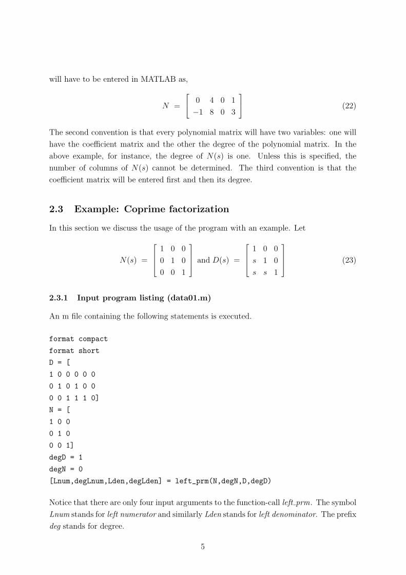
will have to be entered in MATLAB as,
N =
0 4 0 1
−1 8 0 3
(22)
The second convention is that every polynomial matrix will have two variables: one will
have the coefficient matrix and the other the degree of the polynomial matrix. In the
above example, for instance, the degree of N(s) is one. Unless this is specified, the
number of columns of N(s) cannot be determined. The third convention is that the
coefficient matrix will be entered first and then its degree.
2.3 Example: Coprime factorization
In this section we discuss the usage of the program with an example. Let
N(s) =
1 0 0
0 1 0
0 0 1
and D(s) =
1 0 0
s 1 0
s s 1
(23)
2.3.1 Input program listing (data01.m)
An m file containing the following statements is executed.
format compact
format short
D = [
1 0 0 0 0 0
0 1 0 1 0 0
0 0 1 1 1 0]
N = [
1 0 0
0 1 0
0 0 1]
degD = 1
degN = 0
[Lnum,degLnum,Lden,degLden] = left_prm(N,degN,D,degD)
Notice that there are only four input arguments to the function-call left prm. The symbol
Lnum stands for left numerator and similarly Lden stands for left denominator. The prefix
deg stands for degree.
5

2.3.2 Output from MATLAB
The following is the resulting output from MATLAB (ex01.out).
D =
1 0 0 0 0 0
0 1 0 1 0 0
0 0 1 1 1 0
N =
1 0 0
0 1 0
0 0 1
degD =
1
degN =
0
Lnum =
Columns 1 through 7
1.0000 0 0 0 0 0 0
0 1.0000 0 -1.0000 0 0 0
0 0 -1.0000 1.0000 1.0000 0 -1.0000
Columns 8 through 9
0 0
0 0
0 0
degLnum =
2
Lden =
1 0 0
0 1 0
0 0 -1
degLden =
0
2.3.3 Result
For N(s) and D(s) as given in Eq. 23, B(s) and A(s) satisfying Eq. 9 are as given below:
B(s) =
1 0 0
−s 1 0
s− s2 s −1
and A(s) =
1 0 0
0 1 0
0 0 −1
(24)
6

2.4 Example: Checking whether a given polynomial matrix is
unimodular
Suppose we want to decide whether a given nonsingular matrix D(s) is unimodular.
Carry out left coprime factorization as given below:
A(s)−1B(s) = I D(s)−1 (25)
Where I is an identity matrix and A is row proper. It is clear that D is unimodular if
and only if A is a constant matrix. This is illustrated with a unimodular D matrix.
2.4.1 Input program listing
The following MATLAB mfile is executed (data02.m).
format compact
format short
D = [1 0 0 0 0 0
0 1 0 1 0 0
0 0 1 1 1 0]
degD = 1
[B,degB,A,degA] = left_prm(eye(3),0,D,degD)
if degA == 0,
’Given matrix D is unimodular’
end
2.4.2 Output from MATLAB
The following is the resulting output (ex02.out).
D =
1 0 0 0 0 0
0 1 0 1 0 0
0 0 1 1 1 0
degD =
1
B =
Columns 1 through 7
1.0000 0 0 0 0 0 0
0 1.0000 0 -1.0000 0 0 0
0 0 -1.0000 1.0000 1.0000 0 -1.0000
Columns 8 through 9
7

0 0
0 0
0 0
degB =
2
A =
1 0 0
0 1 0
0 0 -1
degA =
0
ans =
Given matrix D is unimodular
2.5 Example: Producing a row proper polynomial
Given a nonsingular polynomial matrix D(s), we wish to find a unimodular matrix W (s),
such that
W (s)D(s) = D(s) (26)
where D(s) is row proper. This is equivalent to finding a left coprime pair D(s), W (s),
such that
D(s)−1W (s) = I D(s)−1 (27)
2.5.1 Input program listing
The following MATLAB mfile is executed (data03.m).
format compact; format short
D = [4 0 12 0 13 0 6 0 1 0
2 2 5 1 4 0 1 0 0 0]
degD = 4
[W,degW,Dhat,degDhat] = left_prm(eye(2),0,D,degD)
2.5.2 Output from MATLAB
The following is the resulting output (ex03.out).
D =
4 0 12 0 13 0 6 0 1 0
2 2 5 1 4 0 1 0 0 0
degD =
8

4
W =
-1.0000 2.0000 0 1.0000
0 1.0000 0 0
degW =
1
Dhat =
Columns 1 through 7
0 4.0000 0 4.0000 0 1.0000 0
2.0000 2.0000 5.0000 1.0000 4.0000 0 1.0000
Column 8
0
0
degDhat =
3
2.6 Programs
The following programs, whose listings appear in alphabetical order in the appendix, are
used in the above-said calculation:
1. left prm.m
2. indep.m
3. makezero.m
4. move.m
5. seshft.m
6. t1calc.m
The user starts the calculation by invoking left prm.m. The following routines of Kwak-
ernaak (1990) are also required:
1. clcoef.m
2. colsplit.m
3. polsize.m
4. rowjoin.m
The program clcoef.m has been modified in this work and its listing also appears in the
appendix. For other routines, the reader is referred to Kwakernaak (1990).
9

3 Aryabhatta’s Identity
In this section, we will find polynomial matrices X(s) and Y (s) satisfying the Arya-
bhatta’s Identity,
X(s)D(s) + Y (s)N(s) = I (28)
given coprime polynomial matrices N(s) and D(s) with D(s) column proper.
3.1 Algorithm (Chang and Pearson, 1982)
Given N(s) and D(s) as given above, go through the entire calculation of Sec. 2 to
compute T1 matrix of Eq. 15 and Eq. 16. In this process, left coprime matrices B(s) and
A(s) can also be computed without much more effort.
As it is given that N(s) and D(s) are coprime with D(s) column proper, there exist
X(s) and Y (s) satisfying Eq. 28 with deg[X(s) Y (s)] < deg[−B(s) A(s)].
Let S denote S matrix of Eq. 17 with all redundant rows deleted. Thus S contains
only independent rows. Thus it is possible to solve
b S = I (29)
After b is found, it is augmented with zero columns at locations corresponding to the
rows of S deleted. Call the matrix thus obtained as T2. As the polynomial equivalent of
this matrix satisfies
T2(s) = [X(s) Y (s)] (30)
X(s) and Y (s) can be calculated.
3.2 Usage
We now illustrate how to use this program with an example. Let
N(s) =
0 4 + s
−1 8 + 3s
and D(s) =
−s 4s + s2
s 0
(31)
3.2.1 Input program listing (data04.m)
An m file containing the following statements is executed.
format compact
format short
D = [
0 0 -1 4 0 1
0 0 1 0 0 0]
10

N = [
0 4 0 1
-1 8 0 3 ]
degD = 2
degN = 1
[Lnum,degLnum,Lden,degLden,Y,degY,X,degX] = left_prm(N,degN,D,degD,2)
Notice that we use the routine left prm.m once again as we did in Sec. 2.3.1. The
same naming convention of variables is used. Notice, however, that there are five input
arguments used in the call to left prm while only four are required in Sec. 2.3.1. The
fifth argument to left prm could be one, two or three. If it is one, coprime factorization
is done. If it is two, Aryabhatta’s Identity is solved. Finally, if it is three, it will try to
solve Eq. 5. In this case, C(s) also required as an input. This is the topic of discussion
in Sec. 4.
3.2.2 Output from MATLAB (ex04.out)
D =
0 0 -1 4 0 1
0 0 1 0 0 0
N =
0 4 0 1
-1 8 0 3
degD =
2
degN =
1
Lnum =
1.0000 1.0000 0 0
8.0000 4.0000 3.0000 2.0000
degLnum =
1
Lden =
0 0 1.0000 0 0 0
0 0 0 4.0000 0 1.0000
degLden =
2
Y =
2.0000 -1.0000 0 -0.2500
0.2500 0 0 0.0625
11

degY =
1
X =
0.7500 0.5000
-0.1875 -0.1250
degX =
0
3.2.3 Result
The results can be summarized as:
B(s) =
1 1
8 + 3s 4 + 2s
A(s) =
s 0
0 4s + s2
(32)
and
X(s) =
0.75 0.5
−0.1875 −0.125
Y (s) =
2 −1− 0.25s
0.25 0.0625
(33)
3.3 Programs
Same as in Sec. 2.6. The user calls left prm.m.
4 Unilateral polynomial matrix equation
In this section, we will find polynomial matrices X(s) and Y (s) satisfying
X(s)D(s) + Y (s)N(s) = C(s) (34)
given polynomial matrices N(s), D(s) and C(s) with D(s) column proper.
4.1 Algorithm (Chang and Pearson, 1982)
There is a solution to Eq. 34 if and only if the greatest common right divisor of D(s) and
N(s) is also a right divisor of C(s).
Let B1(s)A1(s)−1 be a right coprime factorization of N(s)D(s)−1, R(s)−1U1(s) a left
coprime factorization of D(s)−1A1(s) and U2(s)−1C2(s) a left coprime factorization of
C(s)R(s)−1. Then Eq. 34 has a solution if and only if U2(s) is row proper and constant.
Once it is determined that a solution exists to Eq. 34, one can solve it using the same
technique used for solving Eq. 28, as discussed in Sec. 3.1. That is, we only have to
substitue C(s) in the place of I.
12

4.2 Usage
We will illustrate the solution to Eq. 34 with two examples.
4.2.1 First example
An m file containing the following statements is executed (data05.m).
format compact
format short
Num = [0 4 0 1
-1 8 0 3]
degNum = 1
Den = [0 0 1 4 0 1
0 0 -1 0 0 0]
degDen = 2
C = [1 0 1 1
0 2 0 1]
degC = 1
[Lnum,degLnum,Lden,degLden,Y,degY,X,degX] = ...
xdync(Num,degNum,Den,degDen,C,degC)
and the following MATLAB results are obtained (ex05.out):
Num =
0 4 0 1
-1 8 0 3
degNum =
1
Den =
0 0 1 4 0 1
0 0 -1 0 0 0
degDen =
2
C =
1 0 1 1
0 2 0 1
degC =
1
Lnum =
1.0000 1.0000 0 0
13

8.0000 12.0000 3.0000 4.0000
degLnum =
1
Lden =
0 0 1 0 0 0
0 0 0 4 0 1
degLden =
2
Y =
2.0000 -1.0000 0 -0.5000
0.5000 0 0 -0.1250
degY =
1
X =
1.5000 1.0000
0.3750 0.5000
degX =
0
4.2.2 Second example
An m file containing the following statements is executed (data06.m).
format compact
format short e
Num = [0 0.828 72.16 0.556
0 0.23 18.05 0.03 ]
degNum = 1
Den = [-1 0 1 0
0 -1 0 1]
degDen = 1
C = [4.002778 0.09749997
-3006.672 -95.99581]
degC = 0
[Lnum,degLnum,Lden,degLden,Y,degY,X,degX] = ...
xdync(Num,degNum,Den,degDen,C,degC)
and the following MATLAB results are obtained (ex06.out):
Num =
0 8.2800e-001 7.2160e+001 5.5600e-001
14

0 2.3000e-001 1.8050e+001 3.0000e-002
degNum =
1
Den =
-1 0 1 0
0 -1 0 1
degDen =
1
C =
4.0028e+000 9.7500e-002
-3.0067e+003 -9.5996e+001
degC =
0
Lnum =
0 8.2800e-001 7.2160e+001 5.5600e-001
0 2.3000e-001 1.8050e+001 3.0000e-002
degLnum =
1
Lden =
-1.0000e+000 0 1.0000e+000 0
0 -1.0000e+000 0 1.0000e+000
degLden =
1
Y =
1.1563e-001 -2.4049e-001
-1.5290e+002 4.4469e+002
degY =
0
X =
-4.0028e+000 -5.7074e-002
3.0067e+003 7.1673e+001
degX =
0
4.3 Programs
In addition to the programs mentioned in Sec. 2.6, we also need
1. cindep.m
15

2. issoln.m
3. xdync.m
The user starts the calculations with xdync.m
5 Generalized Aryabhatta’s Identity
Given matrices as given in Eq. 35, N(s), D(s) not necessarily coprime, D(s) nonsingular,
H(s) = N(s)D(s)−1 (35)
find matrices in the following generalized Aryabhatta’s Identity: A(s) B(s)
−Y1(s) X1(s)
X(s) −B1(s)
Y (s) A1(s)
=
I 0
0 I
(36)
with
A(s)−1B(s) = B1(s)A1(s)−1 = H(s) (37)
5.1 Algorithm (Chang and Pearson, 1982)
Using the algorithms developed earlier, one can compute the required matrices in three
steps:
5.1.1 Step1: Find A(s) and B(s)
Given H(s) = N(s)D(s)−1 find A(s) and B(s) satisfying Eq. 37. This is done using the
procedure explained in Sec. 2. A(s) and B(s) are left coprime and A(s) is row proper.
5.1.2 Step2: Find A1(s), B1(s), X(s) and Y (s)
Starting from A(s) and B(s) left coprime, A(s) row proper, calculate right coprime
A1(s) and B1(s) satisfying Eq. 37 with A1(s) column proper. Also solve the following
Aryabhatta’s Identity for X(s) and Y (s):
A(s)X(s) + B(s)Y (s) = I (38)
These calculations are carried out by transposing A(s) and B(s), using the procedure
outlined in Sec. 2 and Sec. 3 and transposing the resulting matrices.
16

5.1.3 Step 3: Find X1(s) and Y1(s)
Using the procedure outlined in Sec. 3, find X1(s) and Y1(s) satisfying the following
Aryabhatta’s idenity:
X1(s)A1(s) + Y1(s)B1(s) = I (39)
5.2 Usage
We will illustrate the solution to Eq. 36 with two examples.
5.2.1 First example
An m file containing the following statements is executed (data07.m).
format compact
format short e
Num = [361 72.3 .2 -17.95 0 0
5.2 .18 2.88 .03 .46 0]
degNum = 2
Den = [10 0 6 0 1 0
0 10 0 6 0 1]
degDen = 2
[A,degA,B,degB,A1,degA1,B1,degB1,X,degX,Y,degY,X1,degX1,Y1,degY1] = ...
arya(Num,degNum,Den,degDen)
and the following MATLAB results are obtained (ex07.out):
Num =
3.6100e+002 7.2300e+001 2.0000e-001 -1.7950e+001 0 0
5.2000e+000 1.8000e-001 2.8800e+000 3.0000e-002 4.6000e-001 0
degNum =
2
Den =
10 0 6 0 1 0
0 10 0 6 0 1
degDen =
2
A =
5.0028e+000 -3.0067e+003 1.0000e+000 0
1.6667e-003 9.9722e-001 0 1.0000e+000
degA =
17

1
B =
-1.3829e+003 -1.7950e+001 0 0
5.7872e-001 3.0000e-002 4.6000e-001 0
degB =
1
A1 =
-4.0000e+000 -2.5000e+000 1.0000e+000 0
2.0000e+001 1.0000e+001 0 1.0000e+000
degA1 =
1
B1 =
2.0000e-001 -1.7950e+001 0 0
-1.7200e+000 -1.1200e+000 4.6000e-001 0
degB1 =
1
X =
0 0
-6.3889e-003 -3.8227e+000
degX =
0
Y =
1.3889e-002 8.3102e+000
-5.5556e-002 9.2593e-002
degY =
0
X1 =
-3.8227e+000 0
-4.2593e-002 0
degX1 =
0
Y1 =
1.3889e-002 8.3102e+000
-5.5556e-002 9.2593e-002
degY1 =
0
18

5.2.2 Second example
An m file containing the following statements is executed (data08.m).
format compact
format short e
Num = [
675 90 70 100 720 228 139 185 282 192 90 108 48 60 23 25 3 6 2 2
16 40 200 128 28 78 130 160 14 49 28 64 2 12 2 8 0 1 0 0
288 0 40 544 328 -80 78 840 136 -76 49 472 26 -22 12 114 2 -2 1 10]
Den = [
120 0 0 0 274 0 0 0 225 0 0 0 85 0 0 0 15 0 0 0 1 0 0 0
0 120 0 0 0 274 0 0 0 225 0 0 0 85 0 0 0 15 0 0 0 1 0 0
0 0 120 0 0 0 274 0 0 0 225 0 0 0 85 0 0 0 15 0 0 0 1 0
0 0 0 120 0 0 0 274 0 0 0 225 0 0 0 85 0 0 0 15 0 0 0 1]
degNum = 4
degDen = 5
[A,degA,B,degB,A1,degA1,B1,degB1,X,degX,Y,degY,X1,degX1,Y1,degY1] = ...
arya(Num,degNum,Den,degDen)
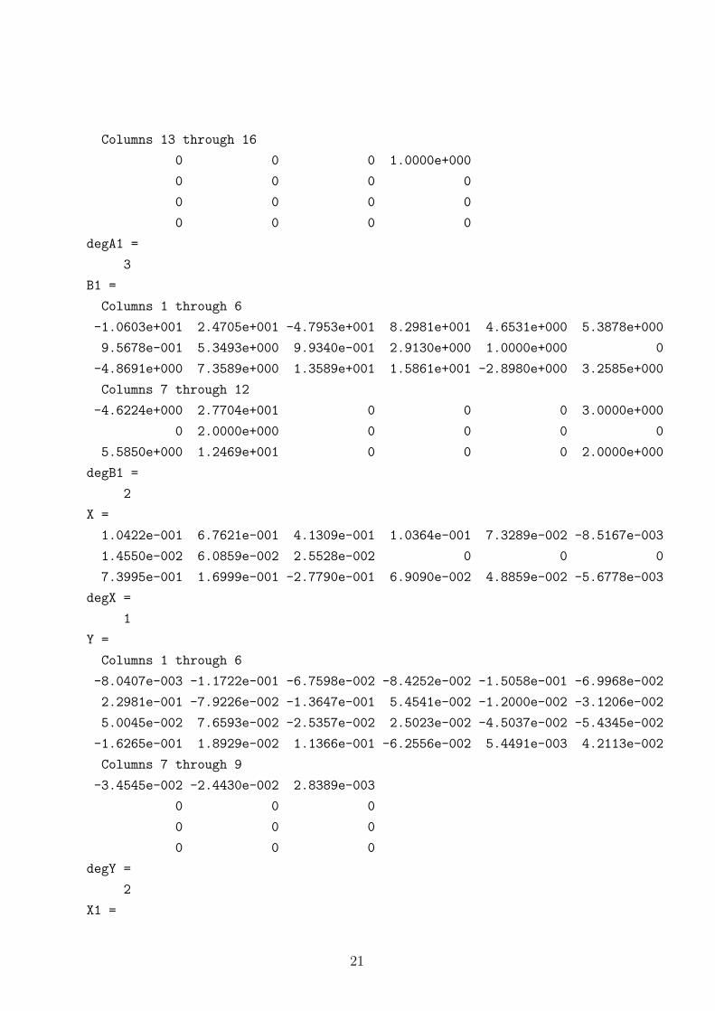
and the following MATLAB results are obtained (ex08.out):
Num =
Columns 1 through 12
675 90 70 100 720 228 139 185 282 192 90 108
16 40 200 128 28 78 130 160 14 49 28 64
288 0 40 544 328 -80 78 840 136 -76 49 472
Columns 13 through 20
48 60 23 25 3 6 2 2
2 12 2 8 0 1 0 0
26 -22 12 114 2 -2 1 10
Den =
Columns 1 through 12
120 0 0 0 274 0 0 0 225 0 0 0
0 120 0 0 0 274 0 0 0 225 0 0
0 0 120 0 0 0 274 0 0 0 225 0
0 0 0 120 0 0 0 274 0 0 0 225
Columns 13 through 24
85 0 0 0 15 0 0 0 1 0 0 0
0 85 0 0 0 15 0 0 0 1 0 0
0 0 85 0 0 0 15 0 0 0 1 0
19

0 0 0 85 0 0 0 15 0 0 0 1
degNum =
4
degDen =
5
A =
Columns 1 through 6
8.0000e+000 -8.5714e-001 -6.0714e-001 1.4000e+001 -1.2857e+000 -8.5714e-001
0 6.0000e+000 -4.5000e+000 0 1.1000e+001 -6.0000e+000
0 0 1.5000e+001 0 0 2.3000e+001
Columns 7 through 12
7.0000e+000 -4.2857e-001 -2.5000e-001 1.0000e+000 0 0
0 6.0000e+000 -1.5000e+000 0 1.0000e+000 0
0 0 9.0000e+000 0 0 1.0000e+000
degA =
3
B =
Columns 1 through 6
4.3429e+001 5.7143e+000 3.0357e+000 3.0000e+000 2.3500e+001 1.2071e+001
-1.0000e+001 2.0000e+000 8.5000e+000 -1.4000e+001 -1.0000e+000 6.0000e+000
3.6000e+001 0 5.0000e+000 6.8000e+001 1.4000e+001 -1.0000e+001
Columns 7 through 12
6.7500e+000 6.5000e+000 3.0000e+000 6.0000e+000 2.0000e+000 2.0000e+000
5.0000e-001 -7.0000e+000 0 1.0000e+000 0 0
6.0000e+000 5.4000e+001 2.0000e+000 -2.0000e+000 1.0000e+000 1.0000e+001
degB =
2
A1 =
Columns 1 through 6
-2.3745e+000 3.6943e+000 -8.0572e+000 1.3912e+001 -2.8235e+000 4.8235e+000
3.5090e+000 3.8856e+000 -1.0644e+001 9.7473e+000 4.8547e+000 1.0908e+000
-5.7623e-002 2.4658e+000 -1.3421e+000 1.2173e+000 -2.8812e-002 3.2329e+000
1.8727e-001 -5.1381e-001 7.3619e+000 -3.9562e+000 7.2029e-002 4.1777e-001
Columns 7 through 12
-1.0265e+001 2.1147e+001 -4.4898e-001 1.1293e+000 -2.2075e+000 8.2347e+000
-2.5916e+000 2.4436e+000 1.0000e+000 0 0 0
-6.7107e-001 6.0864e-001 0 1.0000e+000 0 0
5.6777e+000 -1.5216e+000 0 0 1.0000e+000 0
20
Columns 13 through 16
0 0 0 1.0000e+000
0 0 0 0
0 0 0 0
0 0 0 0
degA1 =
3
B1 =
Columns 1 through 6
-1.0603e+001 2.4705e+001 -4.7953e+001 8.2981e+001 4.6531e+000 5.3878e+000
9.5678e-001 5.3493e+000 9.9340e-001 2.9130e+000 1.0000e+000 0
-4.8691e+000 7.3589e+000 1.3589e+001 1.5861e+001 -2.8980e+000 3.2585e+000
Columns 7 through 12
-4.6224e+000 2.7704e+001 0 0 0 3.0000e+000
0 2.0000e+000 0 0 0 0
5.5850e+000 1.2469e+001 0 0 0 2.0000e+000
degB1 =
2
X =
1.0422e-001 6.7621e-001 4.1309e-001 1.0364e-001 7.3289e-002 -8.5167e-003
1.4550e-002 6.0859e-002 2.5528e-002 0 0 0
7.3995e-001 1.6999e-001 -2.7790e-001 6.9090e-002 4.8859e-002 -5.6778e-003
degX =
1
Y =
Columns 1 through 6
-8.0407e-003 -1.1722e-001 -6.7598e-002 -8.4252e-002 -1.5058e-001 -6.9968e-002
2.2981e-001 -7.9226e-002 -1.3647e-001 5.4541e-002 -1.2000e-002 -3.1206e-002
5.0045e-002 7.6593e-002 -2.5357e-002 2.5023e-002 -4.5037e-002 -5.4345e-002
-1.6265e-001 1.8929e-002 1.1366e-001 -6.2556e-002 5.4491e-003 4.2113e-002
Columns 7 through 9
-3.4545e-002 -2.4430e-002 2.8389e-003
0 0 0
0 0 0
0 0 0
degY =
2
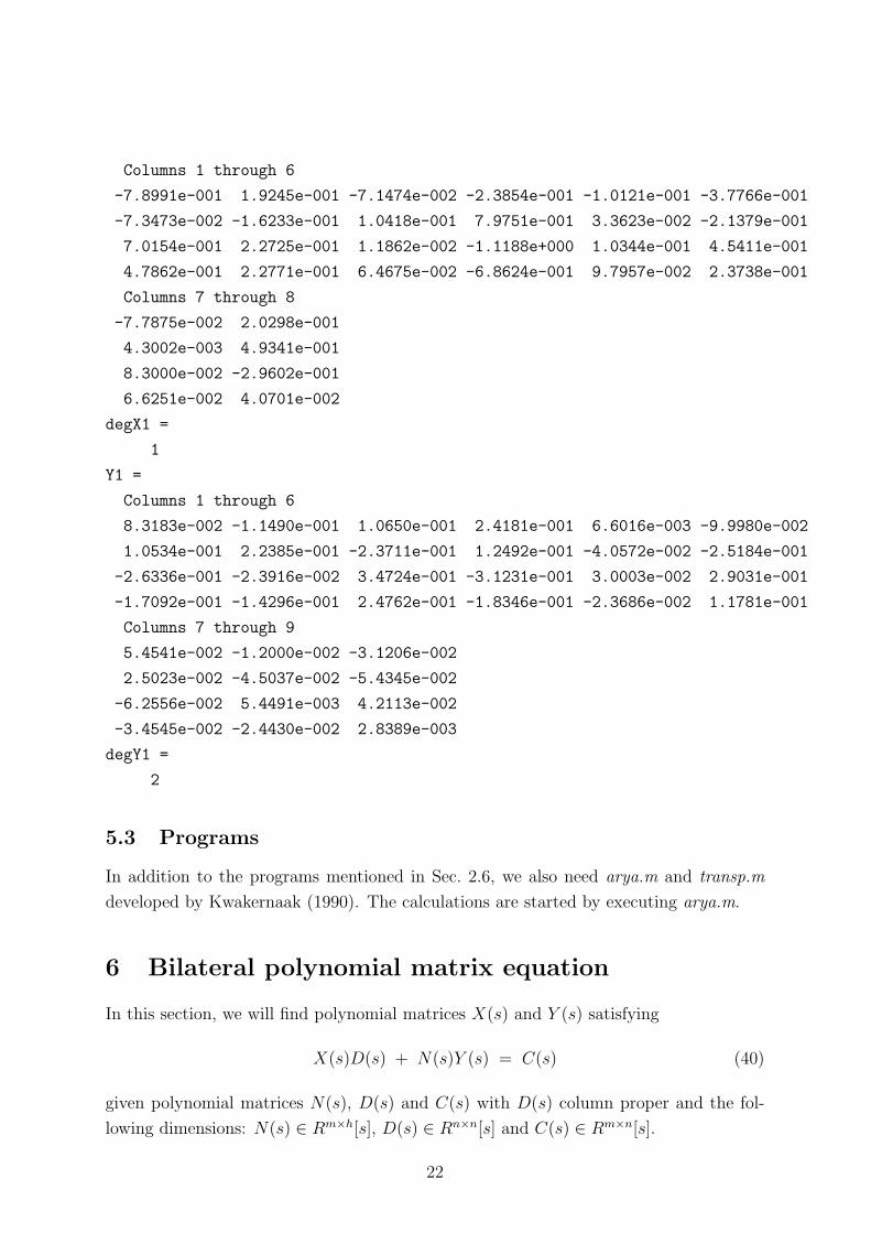
X1 =
21
Columns 1 through 6
-7.8991e-001 1.9245e-001 -7.1474e-002 -2.3854e-001 -1.0121e-001 -3.7766e-001
-7.3473e-002 -1.6233e-001 1.0418e-001 7.9751e-001 3.3623e-002 -2.1379e-001
7.0154e-001 2.2725e-001 1.1862e-002 -1.1188e+000 1.0344e-001 4.5411e-001
4.7862e-001 2.2771e-001 6.4675e-002 -6.8624e-001 9.7957e-002 2.3738e-001
Columns 7 through 8
-7.7875e-002 2.0298e-001
4.3002e-003 4.9341e-001
8.3000e-002 -2.9602e-001
6.6251e-002 4.0701e-002
degX1 =
1
Y1 =
Columns 1 through 6
8.3183e-002 -1.1490e-001 1.0650e-001 2.4181e-001 6.6016e-003 -9.9980e-002
1.0534e-001 2.2385e-001 -2.3711e-001 1.2492e-001 -4.0572e-002 -2.5184e-001
-2.6336e-001 -2.3916e-002 3.4724e-001 -3.1231e-001 3.0003e-002 2.9031e-001
-1.7092e-001 -1.4296e-001 2.4762e-001 -1.8346e-001 -2.3686e-002 1.1781e-001
Columns 7 through 9
5.4541e-002 -1.2000e-002 -3.1206e-002
2.5023e-002 -4.5037e-002 -5.4345e-002
-6.2556e-002 5.4491e-003 4.2113e-002
-3.4545e-002 -2.4430e-002 2.8389e-003
degY1 =
2
5.3 Programs
In addition to the programs mentioned in Sec. 2.6, we also need arya.m and transp.m
developed by Kwakernaak (1990). The calculations are started by executing arya.m.
6 Bilateral polynomial matrix equation
In this section, we will find polynomial matrices X(s) and Y (s) satisfying
X(s)D(s) + N(s)Y (s) = C(s) (40)
given polynomial matrices N(s), D(s) and C(s) with D(s) column proper and the fol-
lowing dimensions: N(s) ∈ Rm×h[s], D(s) ∈ Rn×n[s] and C(s) ∈ Rm×n[s].
22

6.1 Algorithm (Chang and Pearson, 1982)
Let x′k, y′k and c′k be the kth row vectors of X(s), Y (s) and C(s) respectively, i.e.
x′k = [xk1 xk2 . . . xkn] k = 1, . . . ,m (41)
y′k = [yk1 yk2 . . . ykn] k = 1, . . . , h (42)
c′k = [ck1 ck2 . . . ckn] k = 1, . . . ,m (43)
where xkj is the element of X(s) at k-th row and j-th column. ykj and ckj are defined in
a similar way. Then Eq. 40 can be transformed to
X(s)D(s) + Y (s)N(s) = C(s) (44)
with the following definitions:
X = [x′1 x′2 . . . x′m] (45)
Y = [y′1 y′2 . . . y′h] (46)
C = [c′1 c′2 . . . c′m] (47)
D = Im ⊗ D (48)
N = N ′ ⊗ In (49)
where ⊗ denotes Kronecker product.
Now Eq. 44 is of the form Eq. 34. Thus the algorithm used in Sec. 4 can be used for
this purpose.
6.2 Usage
We will illustrate the solution to Eq. 40 with two examples.
6.2.1 First example
An m file containing the following statements is executed (data09.m).
format compact
format short
Num = [-16 8 0 4
-4 0 0 1]
degNum = 1
Den = [0 0 -1 4 0 1
0 0 1 0 0 0]
degDen = 2
C = [1 0 1 1
23

0 2 0 1]
degC = 1
[Y,degY,X,degX] = xdnyc(Num,degNum,Den,degDen,C,degC)
and the following MATLAB results are obtained (ex09.out):
Num =
-16 8 0 4
-4 0 0 1
degNum =
1
Den =
0 0 -1 4 0 1
0 0 1 0 0 0
degDen =
2
C =
1 0 1 1
0 2 0 1
degC =
1
Y =
0 -0.5000 0 -0.1250
0.1250 -1.0000 0 -0.3750
degY =
1
X =
1.5000 2.0000
0.3750 0.2500
degX =
0
6.2.2 Second example
An m file containing the following statements is executed (data10.m).
format compact
format short
Num = [
1 0
1 1]
24

degNum = 0
Den = [
1 0 0 0 0 -1 0 0 0 0 0 0 0 0 0
0 1 0 0 0 0 0 0 0 0 0 0 0 0 0
0 0 1 0 0 0 0 0 0 0 0 0 0 0 0
0 0 0 1 0 0 0 0 -2 0 0 0 0 1 0
0 0 0 0 1 0 0 0 0 -1 0 0 0 0 0]
degDen = 2
C = [
0 0 0 -3 0 1 0 0 2 0
0 0 0 0 -1 0 0 0 0 0]
degC = 1
[Y,degY,X,degX] = xdnyc(Num,degNum,Den,degDen,C,degC)
and the following MATLAB results are obtained (ex10.out):
Num =
1 0
1 1
degNum =
0
Den =
Columns 1 through 12
1 0 0 0 0 -1 0 0 0 0 0 0
0 1 0 0 0 0 0 0 0 0 0 0
0 0 1 0 0 0 0 0 0 0 0 0
0 0 0 1 0 0 0 0 -2 0 0 0
0 0 0 0 1 0 0 0 0 -1 0 0
Columns 13 through 15
0 0 0
0 0 0
0 0 0
0 1 0
0 0 0
degDen =
2
C =
0 0 0 -3 0 1 0 0 2 0
0 0 0 0 -1 0 0 0 0 0
degC =
25

1
Y =
Columns 1 through 7
1.0000 0 0 -3.0000 0 0 0
-1.0000 0 0 3.0000 -1.0000 0 0
Columns 8 through 10
0 2.0000 0
0 -2.0000 0
degY =
1
X =
-1.0000 0 0 0 0
0 0 0 0 0
degX =
0
6.3 Programs
In addition to the programs mentioned in Sec. 2.6, we also need the following:
1. flat2nor.m
2. nor2flat.m
3. polksca.m
4. scakpol.m
5. xdync.m
and transp.m developed by Kwakernaak (1990). The user initiates the calculations with
xdync.m.
7 Numerical issues
The most crucial step in computing coprime factorization is the determination of lin-
ear dependence. We have used the singular values to detect the occurrence of linear
dependence. We also use a zeroing strategy to make small terms zero.
26

7.1 Linear dependence
Suppose we want to check whether the mth row of an m× n matrix A is dependent on
the previous m−1 rows. It is assumed that the first m−1 rows are linearly independent.
Compute the singular values of A. Let σ be the maximum and σ be the minimum of
these. If
σ/σ < ε×max(m, n)
then mth row is dependent on the rest. Here ε is the machine epsilon. Suppose the above
condition is violated. Then we carry out the following test to confirm that the rows are
independent. Let the singular values be arranged in descending order. If the ratio of
the successive singular values is larger than a large number G, we take the rows to be
independent. In our calculations, we have taken the default value of G to be 108, but
the user can override it. This is implemented in the routines that check independence,
namely indep.m, Sec. A.5 and cindep.m, Sec. A.2.
7.2 Zeroing small entries
Small entries of a vector are made zero with the procedure as suggested by Chang, (1982).
The absolute values of the vector are arranged in descending order. If the ratio of two
successive entries is greater than a large number G, we zero all succeeding entries, starting
from the smaller of the two. We have chosen this large number to the same as the one
discussed in the previous sub-section. This is implemented in Sec. A.9.
27

A MATLAB routines
All the m files developed in this work are listed in this section. These are listed under the
heading local routines . We have listed two routines from the work of Kwakernaak (1990)
because we have modified them in the current work. These are clcoef.m and l2r.m. In
the following, we also list the names of functions called by each routine. We have also
listed the functions that came with MATLAB. These have been listed under the heading
Routines of mathworks.
A.1 arya.m
A.1.1 Purpose
Used to solve generalized Aryabhatta’s Identity, Eq. 36.
A.1.2 mfiles called
Local routines: left prm.
Kwakernaak’s routines: transp.
A.1.3 Listing of the code
% function ..
% [A,degA,B,degB,A1,degA1,B1,degB1,X,degX,Y,degY,X1,degX1,Y1,degY1] ...
% = arya(N,degN,D,degD)
% calculates the entries of generalized aryabhatta identity
% -1
% given H = N * D not necessarily coprime,
% finds A, B, A1, B1, X, Y, X1 and Y1 such that V * W = I, where
%
% ( A B ) ( X -B1 )
% V = ( ) and W = ( )
% ( -Y1 X1 ) ( Y A1 )
% -1 -1
% and H = A * B = B1 * A1 , A, B left coprime and B1, A1 right coprime
%
function [A,degA,B,degB,A1,degA1,B1,degB1,X,degX,Y,degY,X1,degX1,Y1,degY1] ...
= arya(N,degN,D,degD,gap)
if nargin==4
gap = 1.0e8;
28

end
[B,degB,A,degA] = left_prm(N,degN,D,degD,1,gap);
[A,degA] = transp(A,degA);
[B,degB] = transp(B,degB);
[B1,degB1,A1,degA1,Y,degY,X,degX] = left_prm(B,degB,A,degA,2,gap);
[B1,degB1] = transp(B1,degB1);
[A1,degA1] = transp(A1,degA1);
[X,degX] = transp(X,degX);
[Y,degY] = transp(Y,degY);
[B,degB,A,degA,Y1,degY1,X1,degX1] = left_prm(B1,degB1,A1,degA1,2,gap);
A.2 cindep.m
A.2.1 Purpose
Checks if the last row of a matrix is dependent on the previous rows and if so, returns
the coefficients of dependence. If independent, the coefficients will be null. See Sec. 7.1.
A.2.2 mfiles called
Local routines: makezero.
Routines of mathworks: norm, svd, /.
A.2.3 Listing of the code
% function b = cindep( S,gap)
% used in XD + YN = C. all rows except the last of are assumed to
% be independent. The aim is to check if the last row is dependent on the
% rest and if so how. The coefficients of dependence is sent in b
function b = cindep( S,gap)
if nargin == 1
gap = 1.0e8;
end
[rows,cols] = size(S);
if rows > cols
ind = 0;
else
sigma = svd(S);
29
len = length(sigma);
if (sigma(len)/sigma(1) <= (eps*max(i,cols)))
ind = 0; % not independent
else
if any(sigma(1:len-1) ./sigma(2:len)>=gap)
ind = 0; % not dependent
else
ind = 1; % independent
end
end
end
if ind
b = [];
else
b = S(rows,:)/S(1:rows-1,:);
b = makezero(b,gap);
end
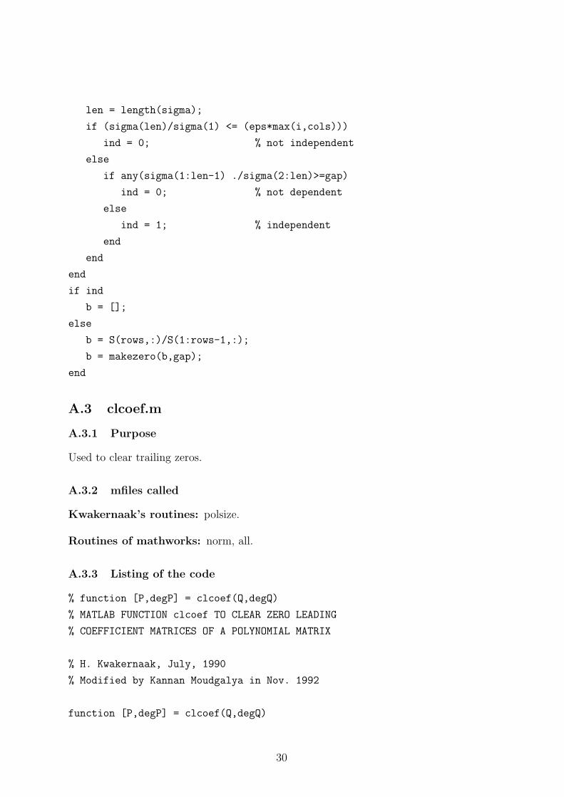
A.3 clcoef.m
A.3.1 Purpose
Used to clear trailing zeros.
A.3.2 mfiles called
Kwakernaak’s routines: polsize.
Routines of mathworks: norm, all.
A.3.3 Listing of the code
% function [P,degP] = clcoef(Q,degQ)
% MATLAB FUNCTION clcoef TO CLEAR ZERO LEADING
% COEFFICIENT MATRICES OF A POLYNOMIAL MATRIX
% H. Kwakernaak, July, 1990
% Modified by Kannan Moudgalya in Nov. 1992
function [P,degP] = clcoef(Q,degQ)
30

[rQ,cQ] = polsize(Q,degQ);
if all(all(Q==0))
P = zeros(rQ,cQ);
degP = 0;
else
P = Q; degP = degQ; rP = rQ; cP = cQ;
j = degP+1;
while j >= 0
if norm(P(:,(j-1)*cP+1:j*cP),inf) < (1e-8)*norm(P,inf)
P = P(:,1:(j-1)*cP);
degP = degP-1;
else
j = 0;
end
j = j-1;
end
end
A.4 flat2nor.m
A.4.1 Purpose
Rearranges a flat (row) polynomial into a polynomial matrix. Opposite of what nor2flat,
Sec. A.11 does.
A.4.2 mfiles called
Routines of mathworks: error.
A.4.3 Listing of the code
% function [X,degX] = flat2nor(flatX,degflatX,rows,bcols)
% returns a flat polynomial X into a polynomial of size rows by bcols
function [X,degX] = flat2nor(flatX,degflatX,rows,bcols)
if length(flatX) == rows * bcols * (degflatX+1)
degX = degflatX;
X = [];
for i = 1:degX+1
31

dummy = zeros(bcols,rows);
dummy(:) = flatX( (i-1)*rows*bcols+1 : i*rows*bcols );
dummy = dummy’;
X = [X dummy];
end
else
error(’flat2nor: dimensions do not agree’)
end
A.5 indep.m
A.5.1 Purpose
Used to check if the rows of a matrix are dependent. If they are dependent, the coefficients
that relate the first dependent row on the previous rows are returned. If the input matrix
is an independent matrix, the coefficient vector will be null. See Sec. 7.1.
A.5.2 mfiles called
Local routines: makezero.
Routines of mathworks: norm, /.
A.5.3 Listing of the code
% function b = indep(S,gap)
% determines the first row that is dependent on the previous rows of S.
% The coefficients of dependence is returned in b
function b = indep( S,gap)
if nargin == 1
gap = 1.0e8;
end
[rows,cols] = size(S);
ind = 1;
i = 2;
while ind & i <= rows
sigma = svd(S(1:i,:));
len = length(sigma);
if(sigma(len)/sigma(1) < (eps*max(i,cols)))
ind =0;
32

else
shsig = [sigma(2:len);sigma(len)];
if any( (sigma ./shsig) > gap)
ind = 0;
else
ind = 1;
i = i+1;
end
end
end
if ind
b =[];
else
c = S(i,:)/S(1:i-1,:);
c = makezero(c,gap);
b = [-c 1];
end
A.6 issoln.m
A.6.1 Purpose
Performs the computations indicated in the beginning of Sec. 4.1 and decides whether
there is a solution to Eq. 34.
A.6.2 mfiles called
Local routines: arya.
Kwakernaak’s routines: modified version of l2r.
A.6.3 Listing of the code
% function soln = issoln(D,degD,C,degC,B,degB,A,degA)
% finds out if there is a solution to the system XD + YN = C
% [-B A] is the left modified minimal basis of [D’ N’]’
function soln = issoln(D,degD,C,degC,B,degB,A,degA)
[B1,degB1,A1,degA1] = l2r(B,degB,A,degA);
[U1,degU1,R,degR] = l2r(A1,degA1,D,degD);
[C2,degC2,U2,degU2] = left_prm(C,degC,R,degR);
if degU2 == 0
33

soln = 1;
else
soln = 0;
end
A.7 l2r.m
A.7.1 Purpose
Carry out left to right coprime factorization. This is a modified version of Kwakernaak’s
routine.
A.7.2 mfiles called
Local routines: arya.
Kwakernaak’s routines: transp.
A.7.3 Listing of the code
% function [Rnum,Rnumdeg,Rden,Rdendeg] = l2r(N,degN,D,degD)
% given Numerator and Denominator polynomial matrices in left form,
% not necessarily coprime, finds right coprime factorisation.
function [Rnum,Rnumdeg,Rden,Rdendeg] = l2r(N,degN,D,degD)
[N,degN] = transp(N,degN);
[D,degD] = transp(D,degD);
[Rnum,Rnumdeg,Rden,Rdendeg] = left_prm(N,degN,D,degD);
[Rnum,Rnumdeg] = transp(Rnum,Rnumdeg);
[Rden,Rdendeg] = transp(Rden,Rdendeg);
A.8 left prm.m
A.8.1 Purpose
Used to produce left coprime factorization given arbitrary right factorization. Used in
all the computations listed in this report.
A.8.2 mfiles called
Local routines: t1calc.
34

Kwakernaak’s routines: rowjoin, polsize, colsplit, clcoef. The last routine has been
modified locally.
Routines of mathworks: nargin, isempty, size, round.
A.8.3 Listing of the code
% function [B,degB,A,degA,Y,degY,X,degX] = ...
% left_prm(N,degN,D,degD,job,gap)
%
% does three different things according to integers that ’job’ takes
% job = 1.
% this is the default. It is always done for all jobs.
% -1 -1 -1
% Given ND , returns coprime B and A where ND = A B
% It is enough if one sends the first four input arguments
% If gap is required to be sent, then one can send either 1 or a null
% entry for job
% job = 2.
% first solve for job = 1 and then solve XA + YB = I
% job = 3.
% used in solving XD + YN = C
% after finding coprime factorization, data are returned
%
% convention: the variable with prefix deg stand for degrees
% of the corresponding polynomial matrices
%
% input:
% N: right fraction numerator polynomial matrix
% D: right fraction denominator polynomial matrix
% N and D are not neccessarily coprime
% gap: variable used to zero entries; default value is 1.0e+8
%
% output
% b and A are left coprime num. and den. polynomial matrices
% X and Y are solutions to Aryabhatta identity, only for job = 2
function [B,degB,A,degA,Y,degY,X,degX] = ...
left_prm(N,degN,D,degD,job,gap)
35

if nargin == 4 | nargin == 5
gap = 1.0e8 ;
end
if nargin == 4, job = 1; end
[F,degF] = rowjoin(D,degD,N,degN);
[Frows,Fbcols] = polsize(F,degF); % Fbcols = block columns
Fcols = Fbcols * (degF+1) ; % actual columns of F
T1 = [];pr =[];degT1 = 0; T1rows = 0;shft = 0;
S=F; sel = ones(Frows,1); T1bcols =1;
abar = (Fbcols + 1):Frows; % a_super_bar of B-C.Chang
while isempty(T1) | T1rows < Frows - Fbcols
Srows = Frows*T1bcols; % max actual columns of result
[T1,T1rows,sel,pr] = ...
t1calc(S,Srows,T1,T1rows,sel,pr,Frows,Fbcols,abar,gap);
[T1rows,T1cols] = size(T1);
if T1rows < Frows - Fbcols
T1 = [T1 zeros(T1rows,Frows)];
T1bcols = T1bcols + 1; % max. block columns of result
degT1 = degT1 + 1; %degree of result
shft = shft +Fbcols;
S = seshft(S,F,shft);
sel = [sel;sel(Srows-Frows+1:Srows)];
rowvec = (T1bcols-1)*Frows+(Fbcols+1):T1bcols * Frows;
abar = [abar rowvec]; % A_super_bar of B-C.chang
end
end
[B,degB,A,degA] = colsplit(T1,degT1,Fbcols,Frows-Fbcols);
[B,degB] = clcoef(B,degB);
B = -B;
[A,degA] = clcoef(A,degA);
if job == 2
S = S(sel,:); % columns
[redSrows,Scols] = size(S);
C = [eye(Fbcols) zeros(Fbcols,Scols-Fbcols)]; % append with zeros
T2 = C/S;
T2 = makezero(T2,gap);
T2 = move(T2,find(sel),Srows);
36

[X,degX,Y,degY] = colsplit(T2,degT1,Fbcols,Frows - Fbcols);
[X,degX] = clcoef(X,degX);
[Y,degY] = clcoef(Y,degY);
elseif job == 3
Y = S;
degY = sel;
X = degT1;
degX = Fbcols;
else
if job ~= 1
error(’Message from left_prm:no legal job number specified’)
end
end
A.9 makezero.m
A.9.1 Purpose
Reduces small entries to zeros. See Sec. 7.2.
A.9.2 mfiles called
Routines of mathworks: find, norm.
A.9.3 Listing of the code
% function B = makezero(B,gap)
% where B is a vector and gap acts as a tolerance
function B = makezero(B,gap)
if nargin == 1
gap = 1.0e8;
end
temp = B(find(B)); % non zero entries of B
temp = -sort(-abs(temp)); % absolute values sorted in descending order
len = length(temp);
ratio = temp(1:len-1) ./temp(2:len); % each ratio >1
min_ind = min(find(ratio>gap));
our_eps = temp(min_ind+1);
37

zeroind = find(abs(B)<=our_eps);
B(zeroind) = zeros(1,length(zeroind));
A.10 move.m
A.10.1 Purpose
Used in rearranging columns of a matrix.
A.10.2 mfiles called
None.
A.10.3 Listing of the code
% function result = move(b,nonred,max)
% Moves matrix b to matrix result with the information on where to move,
% decided by the indices of nonred.
% The matrix result will have as many rows as b has and max number of columns.
% b is augumented with zeros to have nonred number of columns;
% The columns of b put into those of result as decided by nonred.
function result = move(b,nonred,max)
[brows,bcols] = size(b);
b = [b zeros(brows,length(nonred)-bcols)];
result = zeros(brows,max);
result(:,nonred’) = b;
A.11 nor2flat.m
A.11.1 Purpose
Flattens a polynomial matrix into a row vector. Opposite of what flat2nor, Sec. A.4 does.
A.11.2 mfiles called
Kwakernaak’s routines: polsize.
A.11.3 Listing of the code
% function [flatX,degflatX] = nor2flat(X,degX)
% flattens a polynomial X and returns it in flatX. All the polynomials
% are in the notation of Kwakernaak
38

% e.g.
% if X = [x1 (first row)
% x2 (second row)
% ...
% xn] (nth row)
%
% flatX = [x1 x2 ... xn]
function [flatX,degflatX] = nor2flat(X,degX)
[Xrows,Xbcols] = polsize(X,degX);
flatX = [];
for i = 1:degX+1
dummy = X(:,(i-1)*Xbcols+1:i*Xbcols);
dummy = dummy’;
flatX = [flatX dummy(:)’];
end
degflatX = degX;
A.12 polksca.m
A.12.1 Purpose
Performs polynomial ⊗ scalar computation. This is required, for example, in Eq. 49. See
also Sec. A.13.
A.12.2 mfiles called
Kwakernaak’s routines: polsize.
Routines of mathworks: kron.
A.12.3 Listing of the code
% function [kD,degkD] = polksca(D,degD,Mat)
% given polynomial matrix D with degree degD and scalar matrix Mat,
% calculates D kron Mat, where kron stands for kronecker tensor product
function [kD,degkD] = polksca(D,degD,Mat)
[Drows,Dbcols] = polsize(D,degD);
kD = [];
for i = 1:degD+1
39

kD = [kD kron(D(:,(i-1)*Dbcols+1:i*Dbcols),Mat)];
end
degkD = degD;
A.13 scakpol.m
A.13.1 Purpose
Performs scalar ⊗ polynomial computation. This is required, for example, in Eq. 48. See
also polksca.m in Sec. A.12.
A.13.2 mfiles called
Kwakernaak’s routines: polsize.
Routines of mathworks: kron.
A.13.3 Listing of the code
% function [kD,degkD] = scakpol(D,degD,Mat)
% given polynomial matrix D with degree degD and scalar matrix Mat,
% calculates Mat kron D, where kron stands for kronecker tensor product
function [kD,degkD] = scakpol(D,degD,Mat)
[Drows,Dbcols] = polsize(D,degD);
kD = [];
for i = 1:degD+1
kD = [kD kron(Mat,D(:,(i-1)*Dbcols+1:i*Dbcols))];
end
degkD = degD;
A.14 seshft.m
A.14.1 Purpose
Position matrix B at the south east corner of A; shift B before positioning. Fill the
undefined entries with zeros.
A.14.2 mfiles called
None.
40

A.14.3 Listing of the code
% function C = seshft(A,B,N)
% given A and B matrices, returns C = [<-A-> 0
% 0 <-B->] with B shifted east by N cols
function C = seshft(A,B,N)
[Arows,Acols] = size(A);
[Brows,Bcols] = size(B);
if N >= 0
B = [zeros(Brows,N) B];
Bcols = Bcols + N;
elseif N < 0
A = [zeros(Arows,abs(N)) A];
Acols = Acols +abs(N);
end
if Acols < Bcols
A = [A zeros(Arows,Bcols-Acols)];
elseif Acols > Bcols
B = [B zeros(Brows,Acols-Bcols)];
end
C = [A
B];
A.15 t1calc.m
A.15.1 Purpose
Calculates rows of T1 matrix as discussed in Sec. 2.1.
A.15.2 mfiles called
Local routines: indep, mod
Routines of mathworks: norm, isempty, any,
A.15.3 Listing of the code
% function [T1,T1rows,sel,pr] = ...
% t1calc(S,Srows,T1,T1rows,sel,pr,Frows,Fbcols,abar,gap)
% calculates the coefficient matrix T1
41

% redundant row information is kept in sel: redundant rows are marked
% with zeros. The undeleted rows are marked with ones.
function [T1,T1rows,sel,pr] = ...
t1calc(S,Srows,T1,T1rows,sel,pr,Frows,Fbcols,abar,gap)
b = 1; % vector of primary red.rows
while (T1rows < Frows - Fbcols) & any(sel==1) & ~isempty(b)
b = indep( S(sel,:),gap); % send selected rows of S
if ~isempty(b)
b = move(b,find(sel),Srows);
j = length(b);
while ~(b(j) & any(abar==j)) % pick largest nonzero entry
j = j-1; % of coeff. belonging to abar
if ~j
fprintf(’\nMessage from t1calc, called from left_prm\n\n’)
error(’Denominator is noninvertible’)
end
end
if ~any(j<pr & rem(pr,Frows) == rem(j,Frows)) % pr(2),pr(1)
T1 = [T1; b]; % condition is not violated
T1rows = T1rows +1; % accept this vector
end % else don’t accept
pr = [pr; j]; % update prime red row info
while j <= Srows
sel(j) = 0;
j = j + Frows;
end
end
end
A.16 xdnyc.m
A.16.1 Purpose
Solves Eq. 40
A.16.2 mfiles called
Local routines: nor2flat, scakpol, polksca, flat2nor, arya.
42

Kwakernaak’s routines: polsize, transp.
A.16.3 Listing of the code
% function [Y,degY,X,degX] = xdnyc(N,degN,D,degD,C,degC)
% solves XD + NY = C
function [Y,degY,X,degX] = xdnyc(N,degN,D,degD,C,degC)
[Crows,Cbcols] = polsize(C,degC);
[Drows,Dbcols] = polsize(D,degD);
[N,degN] = transp(N,degN);
[Nrows,Nbcols] = polsize(N,degN);
[Ctilda,degC] = nor2flat(C,degC);
[Dtilda,degD] = scakpol(D,degD,eye(Crows));
[Ntilda,degN] = polksca(N,degN,eye(Drows));
[B,degB,A,degA,Ytilda,degY,Xtilda,degX] = ...
xdync(Ntilda,degN,Dtilda,degD,Ctilda,degC);
[X,degX] = flat2nor(Xtilda,degX,Crows,Drows);
[Y,degY] = flat2nor(Ytilda,degY,Nbcols,Cbcols);
A.17 xdync.m
A.17.1 Purpose
Solves Eq. 34
A.17.2 mfiles called
Local routines: t1calc.
Kwakernaak’s routines: colsplit, clcoef.
Routines of mathworks: norm, size, /.
A.17.3 Listing of the code
% function [B,degB,A,degA,Y,degY,X,degX] = xdync(N,degN,D,degD,C,degC,gap)
% given coefficient matrix in T1, primary redundant row information sel,
% solves XD + YN = C
%
function [B,degB,A,degA,Y,degY,X,degX] = xdync(N,degN,D,degD,C,degC,gap)
if nargin == 6
43

gap = 1.0e+8;
end
[F,degF] = rowjoin(D,degD,N,degN);
[Frows,Fbcols] = polsize(F,degF); %Fbcols = block columns
[B,degB,A,degA,S,sel,degT1,Fbcols] = left_prm(N,degN,D,degD,3,gap);
if issoln(D,degD,C,degC,B,degB,A,degA)
[Crows,Ccols] = size(C);
[Srows,Scols] = size(S);
S = S(sel,:);
T2 =[];
for i = 1:Crows,
Saug = seshft(S,C(i,:),0);
b = cindep(Saug);
b = move(b,find(sel),Srows);
T2 =[T2; b];
end
else
error(’message from xdync:No Solution.’)
end
[X,degX,Y,degY] = colsplit(T2,degT1,Fbcols,Frows-Fbcols);
[X,degX] = clcoef(X,degX);
[Y,degY] = clcoef(Y,degY);
References
[1] Astrom, K. J. and Wittenmark, B., “Computer Controlled Systems - Theory and
Design”, Prentice Hall, Englewood Cliffs, NJ 2rd Edition, 1990.
[2] Chang, B-C and Pearson, J. B., “Algorithms for the Solution of Polynomial Equa-
tions arising in Multivariable Control Theory”, Tech. Report No. 8208, Electrical
Engineering Dept., Rice University, May 1982.
[3] Chang, B-C., “Programs for Solving Polynomial Equations” Tech. Report No. 8209,
Electrical Engineering Dept., Rice University, May 1982.
[4] Cheng, L. and Pearson, J. B., “Synthesis of Linear Multivariable Regulators”, IEEE
Trans. Auto. Control, AC-26, pp. 194-202, 1981.
[5] Grimble, M. J. and Kucera, V. (Eds), “Polynomial Methods for Control System
Design”, Springer, London, 1996.
44

[6] Hunt, K. J., “Polynomial Methods in Optimal Control and Filtering”, Peter Pere-
grinus Ltd., London, 1993.
[7] Kailath, T., “Linear Systems”, Prentice-Hall, Inc., Englewood Cliffs, 1980.
[8] Kucera, V., “Discrete Linear Control: The Polynomial Equation Approach”, John
Wiley & Sons, Prague, 1979.
[9] Kwakernaak, H., “MATLAB Macros for Polynomial H∞ Control System Optimiza-
tion”, Memorandum No. 881, Faculty of Applied Mathematics, University of Twente,
Sept. 1990.
[10] Pearson, J. B., “Notes on `1-Optimal Control”, in H∞-Control Theory, Lecture
Notes in Mathematics, 1496, Ed. E. Mosca and L. Pandolfi, Springer-Verlag, Berlin,
1991.
[11] Vidyasagar, M., “Control System Synthesis”, MIT Press, Cambridge, 1985.
[12] Willems, J. C., “Paradigms and Puzzles in the Theory of Dynamical Systems”, IEEE
Trans. Auto. Cont., AC-36, pp. 259-294.
45