mathematics for dynamicists - lecture notes
TRANSCRIPT

HAL Id: cel-01128826https://hal.archives-ouvertes.fr/cel-01128826
Submitted on 10 Mar 2015
HAL is a multi-disciplinary open accessarchive for the deposit and dissemination of sci-entific research documents, whether they are pub-lished or not. The documents may come fromteaching and research institutions in France orabroad, or from public or private research centers.
L’archive ouverte pluridisciplinaire HAL, estdestinée au dépôt et à la diffusion de documentsscientifiques de niveau recherche, publiés ou non,émanant des établissements d’enseignement et derecherche français ou étrangers, des laboratoirespublics ou privés.
Mathematics for Dynamicists - Lecture NotesThomas Michelitsch
To cite this version:Thomas Michelitsch. Mathematics for Dynamicists - Lecture Notes. Doctoral. Mathematics forDynamicists, France. 2006. �cel-01128826�

Mathematics for Dynamicists
Lecture Notes
c© 2004-2006 Thomas Michael Michelitsch1
Department of Civil and Structural Engineering
The University of Sheffield
Sheffield, UK
1Present address : http://www.dalembert.upmc.fr/home/michelitsch/
.
Dedicated to the memory of my parents Michael and Hildegard Michelitsch
Handout Manuscript with Fractal Cover Picture by Michael Michelitschhttps://www.flickr.com/photos/michelitsch/sets/72157601230117490
1
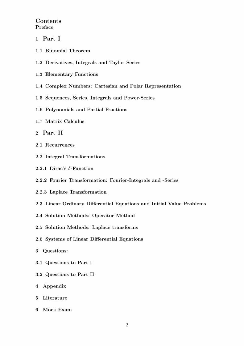
ContentsPreface
1 Part I
1.1 Binomial Theorem
1.2 Derivatives, Integrals and Taylor Series
1.3 Elementary Functions
1.4 Complex Numbers: Cartesian and Polar Representation
1.5 Sequences, Series, Integrals and Power-Series
1.6 Polynomials and Partial Fractions
1.7 Matrix Calculus
2 Part II
2.1 Recurrences
2.2 Integral Transformations
2.2.1 Dirac’s δ-Function
2.2.2 Fourier Transformation: Fourier-Integrals and -Series
2.2.3 Laplace Transformation
2.3 Linear Ordinary Differential Equations and Initial Value Problems
2.4 Solution Methods: Operator Method
2.5 Solution Methods: Laplace transforms
2.6 Systems of Linear Differential Equations
3 Questions:
3.1 Questions to Part I
3.2 Questions to Part II
4 Appendix
5 Literature
6 Mock Exam
2

Preface
These notes are the essence of the lecture series ”Mathematics of Dynamicists” startedin November 2004 and held regularly at the University of Sheffield as a MSc coursemodule.
The module ”Mathematics for Dynamicists” addresses to any students of En-gineering and Natural Sciences who are interested in mathematical-analytical solutionmethods to tackle problems in physics and engineering dynamics.
The lecture notes consist of two parts. Part I is a warmup of the basic mathemat-ics which is prerequisite for the understanding of part II. Some students will be familiarwith the basics reviewed in part I, however the experience showed that it is useful torepeat these basics before starting with dynamical problems of engineering which aredescribed by Recurrences and Ordinary Differential Equations in part II. To ensure theappropriate maths level needed for part II, the reader is highly recommended to answerthe questions to part I before going to part II.
Part II is the essential part and gives a brief introduction to the theory andsolution methods for linear recurrences, Ordinary Differential Equations (ODEs) andInitial Value Problems (IVPs) which are also referred to as Cauchy Problems. Themain goal is less to give proofs but more on applications of the methods on dynamicalproblems relevant to physical and engineering sciences.
Instead of strict proofs we rather confine to short derivations with emphasis onapplications of the analytical techniques. The reader is referred to the standard literaturefor any further proofs which are beyond the scope of these lecture notes.
The selection of materials for this short-term module (2 weeks time) can only bean incomplete and sometimes arbitrary selection of materials. To improve the syllabus,suggestions from anybody are highly appreciated. The enclosed lecture notes are con-tinuously updated and extended. Any communicated discrepancies and errors will becorrected steadily2.
I am especially grateful to my wife Dr. Jicun Wang for proof-reading thismanuscript, to Mr. Shahram Derogar (Dept. Civil & Struct. Eng., Univ. of Sheffield)and to Dr. Andrzej F. Nowakowski (Dept. of Mech. Eng., Univ. Sheffield) for theirhelpful critical comments and valuable inputs which significantly improved the contentsof this lecture.
Sheffield, November 2006 Thomas Michael Michelitsch
2Email: [email protected] , Phone: ++44 (0)114 22 25765 , Fax: ++44 (0)114 22 25700
3

1 Part I
In this section we give a brief repetition of the basic maths which is prerequisite tounderstand the dynamical problems and their solution methods introduced in part II.
1.1 Binomial Theorem
In this section we derive the expansion of (a+b)n in terms akbn−k where a, b are arbitrarycomplex numbers and n is an integer (n = 0, 1, 2, ..,∞). For n = 1, we have
(a+ b)0 = 1 (1)
(a+ b)1 = a + b (2)
for n=2
(a+ b)2 = (a+ b)(a + b) = (0 + 1)a2 + (1 + 1)ab+ (1 + 0)b2 = a2 + 2ab+ b2 (3)
for n = 3
(a+b)3 = (a+b)(a+b)2 = (0+1)a3+(1+2)a2b+(2+1)ab2+(1+0)b3 = a3+3a2b+3ab2+b3
(4)and for general n = 0, 1, 2, ..., we have
(a+ b)n =n∑
k=0
Cn,kakbn−k (5)
We here observe that
C(n, k) = C(n− 1, k) + C(n− 1, k − 1) (6)
and with C(n, n) = C(n, 0) = 1. Relation (6) can be visualized in terms of Pascal’striangle. Hence we have for k = 1 and arbitrary n ≥ 1
C(n, 1) = C(1, 1) + C(1, 0) + C(2, 0) + ..+ C(n− 1, 0) = 1 + 1 + ..+ 1︸ ︷︷ ︸
n times
= n (7)
for k = 2 and arbitrary n ≥ 2
C(n, 2) = C(2, 2)+C(2, 1)+C(3, 1)+ ..+C(n−1, 1) = 1+2+ ..+n−1 =n(n− 1)
2(8)
for k = 3 and arbitrary n ≥ 3
C(n, 3) = C(3, 3) + C(3, 2) + C(4, 2) + ..+ C(n− 1, 2) =2× 1
2+
3× 2
2+ ..+
(n− 1)(n− 2)
2=
n(n− 1)(n− 2)
2× 3
(9)
... for arbitrary k ≤ n.
C(n, k) = C(k, k)+C(k, k−1)+C(k+1, k−1)+..+C(n−1, k−1) =n(n− 1)...(n− k + 1)
1× 2..× k(10)
4

where C(n, 0) = C(n, n) = 1 and moreover C(n, k) = C(n, n − k). When we introducethe factorial function, then we have ”m-factorial” being defined as
m! = 1× 2× ..× (m− 1)×m (11)
and further it is convenient to define 0! = 1. Taking into account that
n(n− 1)..(n− k + 1)︸ ︷︷ ︸
k factors
=n!
(n− k)!(12)
Then we have that (where we introduce the notation a1 + a2 + .. + an =n∑
k=0
ak)
(a+ b)n =n∑
k=0
n!
(n− k)!k!akbn−k (13)
where one defines 0! = 1. The binomial coefficientn!
(n− k)! k!often is also denoted in
the form ofn!
(n− k)!k!=
(
n
k
)
=
(
n
n− k
)
(14)
and referred to as n over k, where
(
n
0
)
=
(
n
n
)
=n!
n! 0!=
n!
n!= 1 (as 0! = 1).
1.2 Derivatives, Integrals and Taylor Series
When we have a function f(t) which we assume to be infinitely often continuously3
differentiable, it is interesting how this function changes when t is increased by a bit,say h. That is we consider
f(t+ h) = f(t) +∫ t+h
tf ′(τ1)dτ1 (15)
where we have introduced the derivative
f ′(τ) =df(τ)
dτ= lim
δ→0
f(τ + δ)− f(τ)
δ(16)
Then we can again put
f ′(τ1) = f ′(t) +∫ τ1
tf ′′(τ2)dτ2 (17)
and a similar relation we have between the n−1th derivative f (n−1) and the nth derivativef (n), namely
f (n−1)(τ) = f (n−1)(t) +∫ τ
tf (n)(τ ′)dτ ′ (18)
Now we put expression for f ′(τ1) (17) into the integral of (15) and obtain
f(t+ h) = f(t) + f ′(t)∫ t+h
tdτ1 +
∫ t+h
tdτ1
∫ τ1
tf ′′(τ2)dτ2 (19)
3A function f(t) is referred to as continuous in a interval x ∈ [a, b] if there is for any ǫ > 0 a δ, sothat f(x+ δ)− f(x) < ǫ.
5
or
f(t+ h) = f(t) + f ′(t)h+ f ′′(t)∫ t+h
tdτ1
∫ τ1
tdτ2 +R2 (20)
f(t+ h) = f(t) + f ′(t)h + f ′′(t)∫ t+h
tdτ1(τ1 − t) +R2
= f(t) + f ′(t)h + f ′′(t)h2
2+R2
(21)
where the remainder term R2 is given by
R2 =∫ t+h
tdτ1
∫ τ1
tdτ2
∫ τ2
tdτ3f
′′′(τ3) (22)
To evaluate R3 we make use of (18) for n = 3, i.e. we replace the variable functionf ′′′(τ3) by the with respect to the τ3-integration constant f ′′′(t) plus remaining integralR3. Then we can write for (22)
R2 = f ′′′(t)∫ t+h
tdτ1
∫ τ1
tdτ2
∫ τ2
tdτ3 +R3
= f ′′′(t)∫ t+h
tdτ1
∫ τ1
tdτ2(τ2 − t) +R3
= f ′′′(t)∫ t+h
tdτ1
(τ1 − t)2
2+R3
= f ′′′(t)h3
3!+R3
(23)
Repeating this process successively, we obtain
f(t+ h) = f(t) + hf ′(t) +h2
2f ′′(t) + ..+ f (n)(t)
hn
n!︸ ︷︷ ︸
Sn
+Rn (24)
where the remainder term is given by
Rn =∫ t+h
tdτ1
∫ τ1
tdτ2..
∫ τn
tdτn+1f
(n+1)(τn+1)︸ ︷︷ ︸
n+1 integrations
(25)
which can be also rewritten as
Rn =∫ t+h
t
(t+ h− τ)n
n!f (n+1)(τ)dτ (26)
If limn→∞Rn = 0, the series Sn converges towards f(t+h). (24) is also known asTaylor Theorem. If the remainder term Rn does not tends to zero, the series expansioncan still be convergent, however not towards the value f(t+ h). Moreover, if we have aconvergent power series
g(t) =∞∑
n=0
antn (27)
which we assume to be convergent, then we find by differentiating (27) at t = 0 the rela-tion between the coefficients an and the derivatives at t = 0, namely an = 1
n!dn
dtnf(t)|t=0.
6

Thus a power series of the form (27) always represents its own Taylor (Mac-Laurin)series. This remains also true for polynomials, i.e. for a series braking with a certainmaximum power tm.
To judge whether or not the remainder term Rn tends to zero for increasing n, weneed not to evaluate Rn explicitly, instead it is sufficient to estimate its value to judgewhether or not it tends to zero when n exceeds all limits. To this end we make use ofthe Mean Value Theorem of integral calculus which says for any in the interval [a, b]continuous function g(x) that
g(x) =1
(b− a)
∫ b
ag(x)dx
∫ b
ag(x)dx = (b− a)g(x)
(28)
where x ∈ [a, b]. Applying this relation to the last integral of (25) or equivalently to (26)we obtain
Rn = f (n+1)(t +Θnh)hn+1
(n+ 1)!(29)
where 0 ≤ Θn ≤ 1 (t +Θnh ∈ [t, t + h]). Hence we have for limn→∞Rn → 0
f(t+ h) =∞∑
k=0
f (k)(t)
k!hk (30)
An expansion the of the form (30) is referred to as a Taylor Series. For the h
range in which the remainder Rn → 0 as n → ∞ tends to zero, Sn→∞ in (24) yieldsexactly f(t + h). Then Sn is an approximation for f(t + h) up to the remainder Rn.Equation (30) is referred to as the Taylor series or Taylor expansion of function f aroundt with respect to h. If we expand around t = 0 then the Taylor series is also referredto as Mac-Laurin series. For any function it has to be checked whether or not theremainder tends to zero for increasing n. There is always only one unique power seriesof a function when expanding it with respect to a variable t. Many functions can beonly defined and computed by Taylor series. Examples include Exponential-function,Logarithm, Hyperbolic and circular (trigonometric) functions. Taylor series have theuseful property that one can generate derivatives and integrals of the function expandedby differentiating the powers of t and integrating powers, respectively. Note that theconcept of Taylor series can also be extended to complex valued functions.Power function: By using (30), we obtain the Mac-Laurin series of (1+ x)α accordingto
(1 + x)α = 1 + αx+α(α− 1)
2!x2 + ..+
α(α− 1)..(α− n + 1)
n!xn +Rn (31)
where α is a real (not necessarily integer) number.The remainder term has the form
Rn =α(α− 1)..(α− n + 1)(α− n)
(n+ 1)!(1 + Θnx)
α−nxn+1 (32)
where 0 ≤ Θn ≤ 1. The remainder obviously tends to zero for xn
(1+Θnx)n≤ xn → 0,i.e.
when |x| < 1. Hence the series
(1+x)α = 1+αx+α(α− 1)
2!x2+ ..+
α(α− 1)..(α− n + 1)
n!xn+ .. =
∞∑
n=0
(
α
n
)
xn (33)
7
Expansion (33) converges for −1 ≤ x ≤ 1 towards (1 + x)α. We observe from(33) that if α = m is an integer, the series (33) coincides with the binomial expansionfor (1 + x)m, breaking with the power xm. In this case it is a sum of a finite number ofterms, holding for any x, not only |x| < 1.
1.3 Elementary functions
In this section we derive some basic functions which are inevitable for our further appli-cations. Generally, Taylor series which are used to compute values of functions.Exponential function: The exponential function describes a growth or decay processwith its change rate being proportional to the value to the value itself. There are a hugeset of examples showing exponential time evolution, among them the time-evolution ofan asset with a certain interest and the decay of an radioactive isotope. Let us assumewe have to a time t = 0 the amount x0 and the bank will give us an interest rate h (100hpercent), then our assets will obey the following recurrence relation4
xn+1 = (1 + h)xn (34)
where xn denotes the amount of money after n years with the initial condition (amountof money at t = 0) x0. (34) is the simplest example for a linear recurrence relation,i.e. xn+1 is a linear function of xn. We shall linear recurrences in more details below.The solution of the recurrence (34) obviously is
xn+1 = (1 + h)nx0 (35)
which gives using the binomial theorem (13) to evaluate (1 + h)n
(1 + h)n =n∑
k=0
n(n− 1)..(n− k + 1)
k!hk (36)
If we introduce a continuous time variable t = nh and consider the limiting case h → 0with t = nh = const thus n = t
h→ ∞, then (36) becomes
(1 + h)n =
n= th∑
k=0
(nh)(nh− h)..(nh− kh+ h)
k!=
n∑
k=0
t(t− h)..(t− kh + h)
k!(37)
in the limiting case h → 0, the powers t(t− h)..(t− kh+ h)︸ ︷︷ ︸
k factors
→ tk andt
h→ ∞ and
hence we obtain
limh→0
(1 + h)
t
h =∞∑
k=0
tk
k!= et (38)
which is the definition of the Exponential function et. Often one denotes it also aset = exp(t), and just calls it the Exponential of t. The series
et =∞∑
k=0
tk
k!(39)
4Without loss of generality our consideration holds for any complex h.
8

which we derived from the binomial theorem is the Taylor series (Mac-Laurin series) ofthis function with respect to t around t = 0. We observe from (39) that its derivativewith respect to t yields the same series, thus
d
dtet = et =
∞∑
k=0
tk
k!(40)
that is y = et solves the differential equationd
dtx = x and correspondingly we find the
solution ofd
dtx = λx is x(t) = eλtx0 (x0 = const).
When we return to our recurrence problem (35), we see that this limiting caseh → 0 when we put xn = x(t) and xn+1 = x(t+ h)
limh→0
x(t + h) = (1 + h)x(t) (41)
or equivalently
limh→0
x(t + h)− x(t)
h= x(t) (42)
The left hand side of this relation is just the definition of the time derivative attime t, namely limh→0
x(t+h)−x(t)h
= dx(t)dt
, thus the recurrence (42) yields in the limitingcase the differential equation
dx
dt= x (43)
which has the solution x(t) = etx0 where x0 is a constant indicating x0 = x(t = 0).Without loss of generality, this consideration remains true also for any starting time t0,
i.e. x(t) = e(t− t0)x(t0). By using the Binomial Theorem (13), we can similarly showas in (36) that
et = limn→∞
(1 +t
n)n (44)
also yields the exponential function. For t = 1, the limiting case of (44) is callede = 1 + 1
1!+ 1
2!+ 1
3!+ .. ≈ 2.7183 Euler number. It is clear that we can represent any
number by a = eln(a) and therefore ax = ex ln(a). Inverting (44) by putting x = et yieldsper definition the natural Logarithm function t = ln(x) and is obtained by the limitingcase
ln (x) = limn→∞
n[x
1
n − 1] (45)
Let us now assume that x = 1 + u with |u| ≤ 1, in order to derive a series forln(1 + u). Then we have5
ln (1 + u) = limn→∞
n[(1 + u)
1
n − 1] (46)
and because of
(1 + u)
1
n = 1 +1
nu+
1
2!(1
n− 1)u2 + ... =
∞∑
k=0
(1n
k
)
uk (47)
5The restriction |u| ≤ 1 is necessary to guarantee the convergence of the series.
9

converging for |u| ≤ 1. As all terms for k ≥ 1 in (47) contain the factor1
n, we can write
for (46)
ln (1 + u) =
= limn→∞
{u+ (1
n− 1)
u2
2!+ (
1
n− 1)(
1
n− 2)
u3
3!+ .. + (
1
n− 1)× ..× (
1
n− k + 1)
uk
k!+ ..}
(48)
thus1
k!(1
n− 1)× ..× ((
1
n− k+1) → 1
k!(−1)k−1(k− 1)! = (−1)k−1 1
kin the limiting case,
thus
ln (1 + u) = u− u2
2+
u3
3− u4
4+ ..+ (−1)k−1u
k
k+ .. (49)
which is the Mac-Laurin series of ln (1 + u) with respect to u converging for −1 < u ≤ 1.The convergence of this series will be discussed in more detail in section 1.5.Hyperbolic functions: Related to the Exponential function are the Hyperbolic func-tions, namely cosh(t), sinh(t) and tanh(t). They are defined as
cosh (t) =1
2(et + e−t)
sinh (t) =1
2(et − e−t)
tanh(t) =sinh(t)
cosh(t)
(50)
or equivalently et = cosh(t) + sinh(t), e−t = cosh(t) − sinh(t). By expanding the expo-nential into a Mac-Laurin series
et =∞∑
n=0
tn
n!= 1 + t +
t2
2+
t3
3!+ .. (51)
and as a consequence of (50) rearranging the terms according to even and odd powersof t, we get
cosh (t) =∞∑
n=0
t2n
(2n)!
sinh (t) =∞∑
n=0
t2n+1
(2n+ 1)!
(52)
where cosh (t) contains only even powers and sinh (t) only odd powers of t. We emphasizethat the definitions of above functions remain also true when t is complex. In the nextsection we give a brief review of complex numbers.
1.4 Complex numbers: Cartesian and polar representation
Cartesian representation of a complex number: Let x and y denote the axis of aCartesian coordinate system, then we introduce the complex number z as follows
z = x+ iy (53)
10

where i =√
(−1) denotes the imaginary unit6 and is conceived to be directed in the
positive y-direction with i2 = −1. (53) is referred to as Cartesian representation of thecomplex number z and x = Re{z} is called the real part of z and y = Im{z} is referredto as the imaginary part of z. Both x and y are real numbers, iy is a imaginary number.A visualization of complex numbers is obtained when we represent them as ”vectors”in the complex plane, where the 1 is the basis vector in positive x-direction and theimaginary unit i the basis vector in positive y-direction.
Complex numbers were first introduced by Gauss, wherefore the complex planeis referred to as Gaussian plane. Complex numbers are together with the Theory ofcomplex functions one of the most crucial tools in mathematics, engineering scienceand physics. To calculate with them is just as with real numbers, but separating realand imaginary parts. Let z1 = x1 + iy2, and z2 = x2 + iy2 be complex numbers, then wecan define the addition the sum of them (addition of complex numbers)
z1 + z2 = x1 + iy1 + x2 + iy2 = x1 + x2 + i(y1 + y2) (54)
and their product (multiplication of complex numbers)
z1z2 = (x1+ iy1)(x2+ iy2) = x1x2+ i2y1y2+ i(x1y2+x2y1) = x1x2−y1y2+ i(x1y2+x2y1)(55)
where we have used i2 = −1. The geometrical interpretation of the multiplication of 2complex numbers becomes clear when performing the multiplication in polar represen-tations shown below. Let z = x+ iy be a complex number, then z∗ = x− iy is referredto as the complex conjugate of z. Sometimes in the literature the complex conjugateis also denoted as z instead of z∗.Polar representation of complex numbers: Let us introduce the polar coordinates
x = ρ cosϕ, y = ρ sinϕ (56)
where ρ =√x2 + y2 and
y
x= tan(ϕ). Then one makes the convention that the angle ϕ
is in the range π < ϕ ≤ π. Other conventions are possible which are equivalent becauseof the 2π-periodicity of the trigonometric functions, for instance 0 ≤ ϕ < 2π. Expressingz in polar coordinates then writes
z = ρ(cosϕ+ i sinϕ) (57)
Now we introduce the exponential function for an imaginary argument iϕ in theform
eiϕ =∞∑
n=0
(iϕ)n
n!(58)
Because of i2m = (−1)m and i2m+1 = i(−1)m we obtain for eiϕ the representation
eiϕ =∞∑
m=0
(−)mϕ2m
(2m)!︸ ︷︷ ︸
cos (ϕ)
+i∞∑
m=0
(−)mϕ2m+1
(2m+ 1)!︸ ︷︷ ︸
sin (ϕ)
= cosϕ+ i sinϕ (59)
or equivalentlycos(ϕ) = cosh (iϕ) = 1
2(eiϕ + e−iϕ)
sin(ϕ) = 1isinh (iϕ) = 1
2i(eiϕ − e−iϕ)
(60)
6In many textbooks, the imaginary unit is denoted as j instead of i.
11

where the hyperbolic functions (60) just indicate just the even and odd parts of theexponential function, respectively.
In view of decomposition (59) into circular (trigonometric) functions, we also canwrite the complex number in the form (57), namely
z = ρ eiϕ (61)
ρ = |z| =√zz∗ is referred to as the modulus of z, and ϕ = arg(z) is referred to as the
argument of the complex number z or sometimes its phase. The exponential eiϕ is alsoreferred to as phase factor. Note that complex conjugation of a phase factor means tochange the sign of its phase, namely (eiϕ)∗ = 1
eiϕ= e−iϕ. Per definition the argument of
the complex number z is within the interval −π < arg(z) ≤ π]. To meet this conventionarg(z) is expressed in terms of the arctan-function (where −π
2< arctan(..) < π
2) in the
formarg(z) = arctan( y
x), if Rez > 0
arg(z) = arctan( yx) + πsign(y), if Rez < 0
(62)
where z = x+ iy and sign(y) = ±1 is the sign of y (y = |y|sign(y)).By using representation(61), it is straight-forward to see the geometrical interpre-
tation of the multiplication of two complex numbers z1 = ρ1 exp iϕ1 and z2 = ρ2 exp iϕ2
z1 · z2 = ρ1ρ2 exp (iϕ1) exp (iϕ2) = ρ1ρ2 exp [i(ϕ1 + ϕ2)] (63)
that is the moduli are being multiplied, whereas the angles are added. Or equivalently:Multiplying a complex number with another complex number means to multiply withits modulus and rotate by its argument.
In the next section we give a brief review of the properties of complex numbers.All considerations of above series and functions remain true in the complex case.
1.5 Sequences, Series, Integrals and Power-Series
In this section we give a brief review of the convergence criteria which are a usefultool to judge whether or not an infinite series converges towards a finite limit. All state-ments on sequences and series made in this paragraph hold also when they are complex.Sequences: Before we start to look at series, let us first give a criteria for the con-vergence of a sequence a0, a1, .., an, .. which is due to Cauchy: the sequence {an} isconvergent an → a if there is for any given ǫ > 0 a nǫ so that |an − a| < ǫ. A simpleexample is the sequence an = 1
nwhich converges towards a = 0.
Series: Let us consider the convergence of series. To this end, we consider first theGeometrical series which can be obtained from (33) for α = −1, namely
(1 + z)−1 = 1− z + z2 − z3 + .. =∞∑
n=0
(−1)nzn (64)
where z can be a complex number z = x + iy. As we know from (33), this series isconvergent for |z| = ρ < 1. The circle ρc = 1, which separates convergent z fromnonconvergent z, is generally referred to as the circle of convergence. For z = −x and|x| < 1 we have that
(1− x)−1 = 1 + x+ x2 + x3 + .. =∞∑
n=0
xn (65)
12
Let us now consider an arbitrary infinite sum of the form
An =n∑
j=0
aj (66)
where aj can be complex numbers. An converges for n → ∞ if there exists a convergentseries
Bn =n∑
j=0
|bj | (67)
with |bn| > |an|∀n, i.e. Bn is an upper limit for An ≤ ∑∞n=0 |an|.
The series An→∞ converges absolutely if the an tends to zero at least as fast as thepower ζn with 0 < ζ < 1. It is a necessary condition that an → 0 for convergence, butnot a sufficient one. An example for a divergent series of this kind is the harmonic series(see question 6). Note an → 0 for n → ∞ does not necessarily indicate that
∑
n an isconvergent!.
From this consideration we obtain the convergence criteria for the series (66):The series An→∞ converges absolutely (absolute convergence means
∑∞n |an|) if there is
a ζ (0 < ζ < 1) where limn→∞ |an| ≤ const ζn or equivalently if
limn→∞
|an|1n < 1 (68)
or as an equivalent criteria
limn→∞
|an+1||an|
< 1 (69)
Criteria (68) is due to Cauchy and (69) is due to D’Alembert. Both criteria are equivalentto each other and indicate absolute convergence, i.e. convergence of
∑∞n |an|.
Integrals: We give the following theorem on the convergence of functions and existenceof integrals: If f(t) is a monotonous function and if the series converges
∞∑
n
f(n) < ∞ (70)
then also the integral∫ ∞
f(t)dt < ∞ (71)
is convergent and vice verse. The lower limit of integration is omitted as it changes theintegral only by a constant and thus does not influence the convergence behavior andthe same is true for the lowest index n0 in series (70). We only need to prove eitherthe sum (70) or the integral (71) being convergent in order to judge the convergence forboth of them. The proof is as follows: Let f(t) be a monotonous decreasing function for0 ≤ t ≤ ∞, then we have that
∞∑
n=1
f(n) ≤∫ ∞
0f(t)dt ≤
∞∑
n=0
f(n) (72)
from which follows if the integral is convergent, it is also the series, and vice versa.Note: If the sequence an → 0 converges towards zero as n → ∞, it is a necessary
however not sufficient condition that∑∞
n an is convergent. An example is the harmonicseries
∑∞n
1nwhich is divergent (see question 6).
13

Power-Series: It is also useful to use above convergence criteria to derive the circle ofconvergence for a complex power series. Consider the series
A(z) =∞∑
j=0
ajzj (73)
where z = ρeiϕ. Applying the above criteria to (73), we have convergence if their termstend to zero faster than a geometrical series. We have convergence for |z| fulfilling
limn→∞
(|z|n|an|)1n = |z||an|
1n < 1 (74)
or
|z| < limn→∞
1
|an|1n
= ρc (75)
or equivalently by using (69), we have convergence when |z| fulfills
limn→∞
|an+1||z|n+1
|an||z|n= |z| |an+1|
|an|< 1 (76)
or
limn→∞
|z| < limn→∞
|an||an+1|
= ρc (77)
Both criteria are equivalent and it depends on the problem to decide which criteria maybe more convenient in order to determine the radius of convergence ρc.In conclusion: A power series
∑∞n=0 anz
n converges if z is within the circle of conver-gence |z| < ρc, which is given by either of the relations (75) and (77). In the casewhen (69) and (77) tend to infinity, the power series is convergent for all z. If theselimiting cases yield zero, it means that the power series is nowhere convergent exceptfor z = 0. Note: (75) and (77) determine the radius of convergence, i.e. it determinesthat within the circle of convergence |z| < ρc, we have convergence. However it doesnot provide information about the behavior of convergence at the circle of convergence,i.e. for |z| = ρc. To judge the convergence on the circle of convergence, additionalconsiderations have to be made. An example is the geometrical series
1
1− x= 1 + x+ x2 + ..+ xn + .. (78)
with convergence circle ρc = 1, i.e. (78) converges for x < 1, but obviously this is nottrue any more for x = 1.To judge the convergence behavior on the circle of convergence, it is often useful toemploy another convergence criteria, which is due to Leibniz saying that: If a series isalternating, i.e. sign(an+1) = −sign(an) and |an| monotonously decreasing |an+1| < |an|with limn→∞ an = 0 tending to zero, then the series
∑∞n an =
∑
n(−1)n|an| is convergent.For instance we can use this criteria to judge what happens on the radius of convergencefor the Logarithm series (49) for u = 1 which is alternating and meeting the Leibnizcriteria, thus
ln(2) = ln (1 + u)|u=1 = 1− 1
2+
1
3− 1
4+ .. + (−1)k−1 1
k+ .. (79)
which converges according to the Leibniz criteria towards ln(2).
14

1.6 Polynomials and Partial Fractions
In this section we give a brief outline of the properties of polynomials and partial frac-tions.Polynomials: Let us consider a polynomial of degree n = 01, 2, ..., where n is an integernumber
P (λ) = λn + an−1λn−1 + ..+ a1λ+ a0 (80)
where the highest power n determines the degree of the polynomial. A fundamentalproperty of polynomials is that they can be factorized in terms of their zeros λi (P (λi) =0), namely
Pn(λ) = (λ− λ1)m1 × ..× (λ− λr)
mr (81)
where mi is referred to as the multiplicity of the zero λi and where n = m1 + .. + mr.If ms = 1 then there is only one factor (λ− λs) in (81). Note that in general the zerosλi of a polynomials are complex numbers. Without loss of generality we have put thecoefficient of λn as equal to one.Partial Fractions: Let Qm(λ) and Pn(λ) be polynomials of degrees m and n, respec-tively, where m < n, then exists a decomposition into partial fractions according to
Qm(λ)
Pn(λ)=
Am1
(λ− λ1)+ ..+
A1
(λ− λm1)m1
+Bm2
(λ− λ2)+ ..+
B1
(λ− λ2)m2+ .. (82)
where λs (s = 1, .., r) denote the r zeros of the denominator Pn(λ) and ms indicate themultiplicity of zeros λs, i.e.
Pn(λ) = Πri (λ− λi)
mi (83)
and Al denote constant coefficients to be determined. It is sufficient to look at the casem < n only, as otherwise we can utilize polynomial division to bring the result intothe form of a polynomial of degree m − n plus a fraction of the form (82). In orderto determine the coefficients A1, .., Am1 we multiply (82) with (λ − λ1)
m1 . Then (82)
assumes the form
(λ−λ1)m1
Qm(λ)
Pn(λ)= Am1(λ−λ1)
m1−1+ ..+A1+(λ−λ1)m1 [
Bm2
(λ− λ2)+ ..+
B1
(λ− λ2)m2+ ..]
(84)Note that the left hand side of this relation is no more zeros λ1 in its denominator (see
(83), Pn(λ)(λ−λ1)m1
= Πri 6=1(λ− λi)
mi). Hence we obtain the coefficients A1, .., Am1 containing
the terms (λ− λ1)−p1 (p1 = 1, .., m1) as
A1 = (λ− λ1)m1
Qm(λ)
Pn(λ)|λ=λ1
A2 =1
1!
d
dλ
{
(λ− λ1)m1
Qm(λ)
Pn(λ)
}
|λ=λ1
..
Am1 =1
(m1 − 1)!
dm−1
dλm−1
{
(λ− λ1)m1
Qm(λ)
Pn(λ)
}
|λ=λ1
(85)
and so forth for all remaining coefficients related to the terms (λ−λs)−ps (ps = 1, .., ms).
The case when the multiplicity of a zero λ1 is equal to one (m1 = 1) is also covered. Inthis case only the first equation (85)1 occurs with m1 = 1.
15
Example: The fraction x2+2x(x−3)3(x+1)
is to be decomposed into partial fractions. According
to (82) we can write
x2 + 2x
(x− 3)3(x+ 1)=
A1
(x+ 1)+
B1
(x− 3)3+
B2
(x− 3)2+
B3
(x− 3)(86)
To handle with partial fractions instead of a representation of the form (82) isoften much more convenient, for instance if we want to integrate such functions. We canfind an antiderivative by integrating its partial fractions, namely
∫dx
(x2 + px+ q)= A1
∫dx
(x− x1)+A2
∫dx
(x− x2)= A1 ln(x−x1)+A2 ln(x−x2)+const
(87)
where xi are the zeros of x2 + px + q, where we have non-multiple zeros p2
4− q 6= 0 is
assumed. In the case of x1 = x2 we have
∫ dx
(x− x1)2= − 1
(x− x1)+ const (88)
1.7 Matrix Calculus
In this section we recall briefly the essentials of matrix calculus with special emphasison eigenvectors and normal forms of matrices.
We confine here to quadratic matrices, which are as a rule sufficient for ourpurposes.Quadratic Matrices: A quadratic n× n matrix A is a scheme
A =
a11, .., a1n.. ..
.. .. ..
an1, .., ann
(89)
Matrices are essential in order to deal with linear recurrences which we shallconsider in the next section. Let ~X = x1e1+..+enxn ∈ Rn be a vector with n componentsxi with the basis vectors ei in the n-dimensional vector space Rn = R× ..×R Normallythe basis vectors ei are chosen in Cartesian representation, namely
ei · ej = δij (90)
where we have introduced the Scalar Product of two vectors ~a,~b according to
~a ·~b = a1b1 + a2b2 + .. + anbn = |~a||~b| cosαa,b (91)
where αa,b is the angle between ~a and ~b and |~a| denotes the modulus of a vector ~a being
defined as |~a| =√
a21 + a22 + ..+ a2n. The condition (90) indicates mutual ortho-normality(it means mutually orthogonal and normalized, i.e. ei ·ei = 1) of the basis vectors whereδij denotes Kronecker δ-symbol being defined as
δij =
{
1; i = j
0; i 6= j(92)
i.e., δ11 = δ22 = .. = δnn = 1, and δ12 = δ13 = ..δn−1,n = 0. For a Cartesian basis{e1, .., en} we have
16

Det(e1, .., en) = 1 (93)
which means that the coordinate system spanned by {e1, .., en} is a rectangular one.(93) represents the volume of the n dimensional unit cube spanned by the ortho-normalbasis vectors. In (93) we have introduced the Determinant of an n×n matrix A = (aij)(i, j = 1, .., n) which is defined by
DetA =∑
σ
(−1)σa1,i1 × ..× an,in (94)
where the summation is performed over all n! permutations of the indices. σ = σ denotesthe number of transpositions (mutual exchanges of indices) necessary to transform thesequence {1, 2, .., n} into the permutated sequence {i1, i2, .., in}.
For example the determinant of a 2× 2 matrix A = (aij (i, j = 1, 2) is given by
DetA = a11a22 − a12a21 (95)
The value of a determinant is a measure for their linear dependence (or indepen-dence). DetA = 0 indicates that A consists of n linear dependent (columns and line)vectors. DetA 6= 0 indicates they are linear independent. What means linear indepen-dence? A useful definition is: The vectors ~X1, ~X2, .., ~Xn are linear independent if thesystem of equations
C1~X1 + C2
~X2 + .. + Cn~Xn = 0 (96)
have no other than the trivial solution C1 = C2 = .. = Cn = 0. Linear independenceof a set of vectors ~Xi ∈ Rn also means that any given vector ~b ∈ Rn can be uniquelyrepresented by a linear combination A1
~X1+..+An~Xn, which means the set ~Xi constitutes
a basis of the vector space Rn with which all vectors of the Rn can be represented. Inthis sense the constants Ai represent the ~Xi-components of vector ~b. If the vectors~X1, ~X2, .., ~Xn are linear independent, i.e. rank{X} = n, (X = ~X1, ~X2, .., ~Xn), then we
can use the set of ~Xi as a basis to span any vector ~Y = (yi) (i = 1, .., n), that is theequation system
C1~X1 + C2
~X2 + ..+ Cn~Xn = ~Y (97)
or in matrix notation X = ( ~X1, .., ~Xn)
X · ~C = ~Y (98)
has one unique solution-vector ~C = (Ci) because of DetX 6= 0 which is crucial to invert(98). Formally we can write the inversion as
~C = X−1~Y (99)
where X−1 is the inverse matrix to X fulfilling the property X ·X−1 = X−1 ·X = I.Further details about solution techniques (Cramer’s rule, Gaussian elimination) whichcan be found in many textbooks. Applying Cramer’s rule, the coefficients Ck of vector~C can equivalently be written as
17
C1 =Det
(
~Y , ~X2, .., ~Xn
)
Det(
~X1, ~X2, .., ~Xn
)
C2 =Det
(
~X1, ~Y , .., ~Xn
)
Det(
~X1, ~X2, .., ~Xn
)
.. ..
Ck =Det
(
~X1, ~X2, .., ~Xk−1, ~Y , ~Xk+1, .. ~Xn
)
Det(
~X1, ~X2, .., ~Xn
)
.. ..
Cn =Det
(
~X1, ~X2, .., ~Xn−1, ~Y)
Det(
~X1, ~X2, .., ~Xn
)
(100)
where the numerators on the right hand sides of the Ck are generated by determinantsof matrices which are obtained when replacing ~Xk by ~Y in X =
(
~X1, ~X2, .., ~Xn
)
.
Rank of a Matrix: In the case of linear independence of the vectors ~X1, ~X2, .., ~Xn
the rank of the matrix X = [ ~X1, ~X2, .., ~Xn] is n. Generally, the rank of a matrix isthe number of linear independent column vectors (coinciding with the number of linearindependent row vectors). For a n×n matrix A with some non-zero elements the rank is
between 1 and n, i.e. 1 ≤ rank(A) ≤ n. If the rank of the n×n matrix ( ~X1, ~X2, .., ~Xn) isr with 1 ≤ r ≤ n, then there exists a n− r parametric solution of (96). For instance for
r = n−1, we have one-parametric solution ~C = (Ci) = C~V (with one parameter C to bearbitrarily chosen). Another observation is useful: If the rank r of an n× n-matrixA is smaller than n, i.e. r < n, then its determinant DetA = 0 is zero.Further matrix operations: A linear relation between two vectors ~X = (xi) and~Y = (yi) means any component yi is a linear combination of the components xi, hence
yi = Ai1x1 + ..+ Ainxn =n∑
j=1
Aijxj , i = 1, .., n (101)
Symbolically we can write this linear relation in matrix form, namely
~Y = A · ~X (102)
indicating the ”multiplication” of a vector with a matrix. When we now assume ~x = B·~w,then we arrive at the multiplication of two matrices A and B, defined by
(A ·B)ij =n∑
k=1
AikBkj (103)
Note in general A ·B 6= B ·A, that is, matrix multiplication is in general non-commutative. The sequence of multiplication is crucial, unlike the case when wemultiply scalar numbers. A little later we will discuss under which conditions the matrixmultiplication is commutative (i.e. can be traced back on scalar multiplication).
Eigenvectors and eigenvalues: In general a vector A · ~X differs by modulus anddirection from vector ~X . That leads us to the question: Are there vectors whose directionremains unchanged when multiplying them with a matrix A? Clearly such vectors depend
18

on matrix A. If ~v represents such a vector, then any scalar multiple const~v of it alsorepresents such a vector. Hence we look for vectors ~v fulfilling
A · ~v = λ~v (104)
A vector fulfilling (104) is referred to as an Eigenvector of matrix A and λ an Eigenvalueof matrix A. Bringing λ~v to the left hand side, (104) can be rewritten as
(A− λI) · ~v = 0 (105)
where I = (δij) is the unity matrix (I ~X = ~X, ∀ ~X)7. We see that ~v is obviously thenontrivial solution vector of the homogeneous system of equations (104). A nontrivial(i.e. nonzero) solution only exists if λ is chosen such that the rank of (A− λI) is atmost n− 1. That means the condition
Det (A− λI) = 0 (106)
for λ needs to be fulfilled. From this condition (106), λ is to be determined. Thiscondition also is referred to as Characteristic Equation. From the definition of thedeterminant follows that P (λ) = (A− λI) is a polynomial of degree n. P (λ) is referredto as the Characteristic Polynomial of the matrix A and (106) is referred to as thecharacteristic equation. Using the properties on polynomials of section 1.6 we know thatP (λ) has n zeros λi. There are now two different possibilities: (i) All zeros of (106)are different, i.e. λi 6= λj for i 6= j; and (ii) we have multiple zeros λs. Let us first ofall discuss case (i), i.e. the multiplicity of any zero λi is equal to 1. We then have n
different equations
(A− λiI) · ~vi = 0 (107)
with n different non-zero eigenvectors ~vi in general8. In the appendix it is shown that if alleigenvalues λi 6= λj for i 6= j then the n eigenvectors ~vi are linear independent and henceconstitute a complete basis of the n-dimensional vector space, i.e. any arbitrary vector~b = (bi) =
∑ni ci~vi can be represented as a unique linear combination of eigenvectors.
Because of DetV 6= 0 (V = (~v1, .., ~vn)), the matrix A has the representation
A = V · D ·V−1 (108)
where
D = diag(λ1, ..λn) = (λiδij) =
λ1 0.. .. 00 λ2 0.. 00 0.. .. 00 .. λn−1 00 0.. 0 λn
n×n
(109)
is the diagonal form (normal form) consisting of the eigenvalues (λ1, .., λn) in the samesequence as V the corresponding eigenvectors (~v1, .., ~vn). (109) is referred to as thediagonal form or diagonal representation of matrix A. The diagonal matrix D is themost simple and natural representation of the matrix A. Again we emphasize that therepresentation (109) exists in general only if we have n linear independent eigenvectors~vi, i.e. if we have enough, namely n eigenvectors that they constitute a complete basisof the Rn. This is always true if the eigenvalues λi are all different and it is sometimes
7∀ abbreviating ”for all”.8Any eigenvector ~vi is only determined up to a constant, i.e. ~vi · const is also a eigenvector ∀ const
19
true if we have multiple eigenvalues (see below). To understand (109) we consider how it
acts on an arbitrary vector ~X which has the unique representation ~X = C1 ~v1+ ..+Cn ~vnin terms of eigenvectors. Then we have that A · ~X = C1λ1 ~v1 + ..+Cnλn ~vn = V · DV−1.
A matrix with det(A) = 0 is called singular thus its inverse does not exist. As
a consequence a system of equations A · ~X = ~b do not have a solution if ~b is linearindependent from the columns of A.Let us now consider the case of multiple (degenerate) eigenvalues. The characteristicpolynomial assumes then the form9
Det (A− λI) = (−1)nr∏
j=1
(λ− λj)mj (110)
where the mj are referred to as the algebraic multiplicity of the eigenvalue λj(withm1 + ..+mr = n). Let λs be an eigenvalue with algebraic multiplicity ms > 1 and
rs = rank (A− λsI) (111)
Now we have the following possible cases:Case (i) rs = n −ms: In this case we can find ms linear independent eigenvectors ~vs
i
i = 1, 2, .., ms fulfilling
(A− λsI) · ~vs = 0 (112)
In this case the situation is in a sense the same as if we would have ms differenteigenvalues: We can find a ms dimensional eigenbasis. If rj = n − mj is true for alleigenvalues λj then a full basis consisting of eigenvectors exist thus the diagonal form ofmatrix A exists.Case (ii) rs = n −ms + δs > n −ms: In this case we can find only n − rs = ms − δs(δs = 0, 1, .., ms − 1) linear independent eigenvectors as solutions of (112) (The caseδs = 0 corresponds to the above case that rs = n−ms. That is in this case there are notenough linear independent eigenvectors which spanning the complete ms-dimensionalspace. In this case there is no basis consisting of eigenvectors thus matrix A is non-diagonalizable. However we can find a basis which transforms matrix A to its mostsimple representation which is the so called Jordan Normal Form, with
A = VJV−1 (113)
where
J =
J1 0.. .. 00 J2 0.. 00 0.. .. 00 .. Jr−1 00 0.. 0 Jr
(114)
where to each eigenvalue λs with multiplicity ms (114) contains n−rs = ms−δs Jordanblocks of the form
9where we introduce the notation∏r
j=1αj = α1α2..αr.
20

Js = λsδij + δi,j−1 =
λs 1.. .. 00 λs 1.. 00 0.. .. 00 .. λs 10 0.. 0 λs
(115)
For more details we refer to the literature.
For the sake of completeness we briefly recall the most important properties ofdeterminants. All relations hold for both cases when the vectors ~Xi are row vectors aswell as column vectors since DetA = DetAtr (where Atr denotes the transposed matrixof A generated by exchange of rows and columns, i.e. (Atr)ij = (A)ji. Then we have
Det(
~X1, ~X2, .. ~Xn
)
= −Det(
~X2, ~X1, .. ~Xn
)
(116)
i.e. to exchange of any two vectors will change the sign of the determinant.
Det(
C1~X1, C2
~X2, .., Cn~Xn
)
= C1 · C2 · .. · Cn
(
~X1, ~X2, .. ~Xn
)
(117)
andDet
(
~X1, C1~X1 + C2
~X3, ~X3.. ~Xn
)
= 0 (118)
i.e. a determinant with linear dependent column or row vectors is vanishing. Moreoverwe have the product rule
Det(A ·B) = (Det(A)) · (Det(B)) (119)
i.e. the determinant of a matrix product is the product of determinants of the matrices.This case includes also (117) when multiplying A with a diagonal matrix. From (119)follows that
Det(A ·A−1) = Det I = Det(A) ·Det(A−1) = 1 (120)
or
Det(A−1) =1
DetA(121)
and similarlyDet(An) = (Det(A))n (122)
When we have a matrix which possesses a diagonal form and hence the repre-sentation A = VDV−1, where D is the diagonal matrix consisting of eigenvalues of theform (108), then it follows that
DetA = Det (VDV−1) = DetD =n∏
i=1
λi (123)
and similarly we have with that
Det(A− λI) = Det(
V(D − λI)V−1)
= Det(D − λI) =n∏
i=1
(λi − λ) (124)
which is indeed the characteristic polynomial Pn(λ) (Eq. (106). Moreover from (122)and (124) we find that
Det(Am) = (Det(A))m =n∏
i=1
λmi (125)
21

Functions of matrices: Let us assume A has a diagonal-form (i.e. the geometricalmultiplicity of all eigenvalues is n) and thus can be represented as A = VDV−1. Let usnow consider the mth power (m = 0,±1,±2, ..)
Am = A · .. ·A︸ ︷︷ ︸
m times
(126)
Because of A = V · D ·V−1, (126) assumes the form
Am = V · D ·V−1 ·V︸ ︷︷ ︸
I
·D ·V−1 · .. ·V · D ·V−1 = V · DmV−1 (127)
where
Dm = diag(λm1 , .., λ
mn ) = (λm
i δij) =
λm1 0.. .. 0
0 λm2 0.. 0
0 0.. .. 00 .. λm
n−1 00 0.. 0 λm
n
(128)
In view of these relations we can define functions of n × n matrices to be alson × n matrices by their Taylor series, namely a scalar function f(λ) has a Mac-Laurinseries according to
f(λ) =∞∑
m=0
amλm, |λ| < ρc (129)
with am = 1m!
dm
dλm f(λ = 0) and converging for λ < ρc. Then the corresponding matrixfunction can be defined by
f(A) =∞∑
m=0
amAm (130)
having the same coefficients as the scalar function (129) and where the scalar variableλ is replaced by matrix A. By using (127) and (128) we can further write (130) in theform
f(A) = V(∞∑
m=0
amDm)V−1, |λi| < ρc (131)
We can evaluate the series f(D) =∑∞
m=0 amDm by taking into account that D isdiagonal and obtain
f(D) =
(∞∑
m=0
amλmi δij
)
=
f(λ1) 0.. .. 00 f(λ2) 0.. 00 0.. .. 00 .. f(λn−1) 00 0.. 0 f(λn)
(132)
We observe that the matrix f(A) has the eigenvalues f(λi) (where λi
are the eigenvalues of A) and the same eigenvectors as A. Note: the powerseries in the diagonals converge only towards the f(λi) if all eigenvalues λi are withinthe circle of convergence ρc of expansion (129), i.e. if the eigenvalue with the maximummodulus is within the circle of convergence Max(|λi|) < ρc. A prominent example of afunction of a matrix B is the exponential being defined as
exp(B) =∞∑
m
Bm
m!(133)
22

with ρc = ∞, i.e. converging ∀λi. Often one considers functions of B = At, where t isa scalar (time) variable. A very useful property of the matrix exp (At) is that it solvesin full analogy to scalar functions the linear differential equation system (where A isassumed to be a constant time independent n× n matrix)
d
dtexp (At) = A · exp (At) (134)
which is easily verified by using the expansion of the exponential. thus the vector~X(t) = exp (At) · ~X0 solves the differential equations system
d
dt~X = A · ~X (135)
with the initial vector ~X(t = 0) = ~X0. This will be important in part II when weconsider systems of differential equations (Sec. (2.6)).
2 Part II
In this section we give an introduction into analytical methods to tackle dynamicalproblems. We consider recurrences which describe discrete dynamical processes andtheir continuous counterpart which are described by Ordinary Differential Equations(ODE’s) and Initial Value Problems (IVPs) with special emphasis on dynamical engi-neering applications and physics. We recall the general theory briefly, but for the sakeof analytical feasibility we mainly confine to dynamical systems which can be describedby ODEs with constant (time independent) coefficients. Fortunately many dynamicalproblems relevant in engineering science and physics are covered by this type.
2.1 Recurrences
Many processes in dynamics can be described by either (i) differential equations or by (ii)recurrences. Differential equations describe processes which evolve continuously in time,whereas recurrences are an appropriate description when we are looking on the timeevolution of a variable X only to certain discrete times tn, i.e. X(tn) = Xn. Examplesare the development of a population which we measure for instance every year at thesame day, or an asset on the bank which grows not continuously. A recurrence can bedescribed as a discrete mapping of the form
Xn+1 = f(Xn, C) (136)
with a given initial value X0 and a so called control parameter C (or even a set of controlparameters). For the definition of recurrences the introduction of a control parameteris not necessary, however in many cases the dynamic behavior of a variable becomesmore clear by considering the dependence of the dynamical behavior of such a controlparameter. f(X,C) can be an arbitrary generally also nonlinear function of X . Anexample for the influence of a control parameter is the growth of a population underthe influence of a variable food supply which enters the dynamic behavior as a controlparameter. The dynamic behavior, i.e. the development of Xn depends on both, theinitial value X0 and on the control parameter C, i.e. Xn = Xn(X0, C). Formally wewrite the solution of (136) in the form
Xn = f(..f(X0, C))︸ ︷︷ ︸
n times
(137)
23

i.e. the initial value X0 is inserted into the function, and the result is again insertedinto the function; this process is performed n times. One also calls such a process whenthe results is again entered into the function itself as iteration or feedback loop. Inmost nonlinear cases (apart from a few exceptions), there is no other possibility as tocompute Xn by performing the (nonlinear) feedback loop n-times which corresponds to(137). As a rule, one cannot predict the long-term dynamic behavior of such a nonlinearrecurrence, (i.e. the behavior after a high number n of loops) of nonlinear mappingsexcept one performs all the n iterations explicitly. This is also reflected by the highsensitivity on the initial conditions X0 of nonlinear recurrence mappings. Thereforenonlinear recurrences are also referred to as deterministic chaotic mappings. Toget an overview on the nonlinear dynamic behavior one needs to perform the iterationson a computer. A prominent example of the most simple nonlinear recurrence is theVerhulst-Equation
Xn+1 = µ(1−Xn)Xn (138)
with control parameter µ. If the behavior for n → ∞ is bounded, i.e. non-divergent,then the sequence Xn (for large n) is referred to as an attractor. In (138) one can findattractors Xn(µ) for 0 < µ < 4 for a certain set of initial conditions. The representationof this attractor vs µ has become famous under the name Feigenbaum diagram, andwas discovered first by Mitchell Feigenbaum about three decades ago. (138) is conceivedas the most simple example for a deterministic chaotic system. If we chose instead ofreal variables Xn complex variables, then nonlinear recurrences generate dynamics withbasins which remain bounded (non-divergent) in both the complex z0-plane of initial val-ues (Julia Set) as well as in the complex c-plane of control parameters (MandelbrotSet) with so called fractal boundaries or simply Fractals. The terminology Fractaland related, the field of Fractal Geometry was first introduced by Benoit Mandelbrotdescribing geometrical objects having non-integer dimensions, indicating their highlyirregular shapes. Mandelbrot was motivated by the wish to create a theory and quanti-tative measure of roughness in order to describe rough surfaces and boundaries quanti-tatively. Fractal objects have the remarkable property of self-similarity, which meansthat zooming into a fractal pattern reveals again a ”similar” looking fractal pattern. As-signing different colors depending how fast a recurrence of the form (136) converges ordiverges can generate fractal images of stunning beauty10. Well-known is the so calledMandelbrot Set generated by the complex mapping zn+1 = z2n + c in the complex c-plane for a constant initial condition z0 = 0 which was first discovered and described byBenoit Mandelbrot. An example for a fractal image which was generated by a complexrecurrence of the form (136) is shown on the cover page of these notes. Unfortunately wecannot devote here more space to the highly challenging field of Nonlinear Dynamics,Chaos Theory, Complex Systems and Fractal Geometry. The interested readeris highly encouraged to further deal with these strongly related subjects. Any supportfor this goal is provided.For the sake of analytical calculability we confine us now to linear recurrences whichcan be solved in closed form, i.e. without performing n iterations explicitly. Linear re-currences, are mappings (136) where F (X,C) is a linear function of X having the formF (X,A,B) = AX +B, where A,B are constant (control) parameters.Linear recurrences: The most simple example of a linear recurrence we already metin section 1.3 (eq. 34)). Similarly, in the general case, a linear recurrence has the form
10Stunning examples of Fractals including downloadable references for further reading, pro-grams and related links can be found in the web at http://michelitsch-fractals.staff.shef.ac.uk andhttp://en.wikipedia.org/wiki/Burning Ship fractal
24

Xn+1 = AXn +B (139)
with a given initial value X0 and control parameters (constants) A,B. Performing then iterations from X0 to Xn leads to
Xn = AnX0 +B(1 + A+ A2 + ..+ An−1)
Xn = AnX0 +B(An − 1)
(A− 1)
(140)
especially for B = 0 (140) yields Xn = AnX0 according to the recurrence Xn+1 = AXn
with given X0.So far we considered in this section dynamical systems of one variable (one-degree offreedom). However, we can also define recurrences for systems characterized by n vari-
ables (multi-degree of freedom systems)which is represented by a vector ~X . In thesecases it is clear that linear recurrences are defined by matrix relations of the form.
~Xn+1 = A · ~Xn +~b (141)
where A is now a N × N matrix. In complete analogy to the scalar case (136), theevaluation of (141) yields analogously to (140) the solution
~Xn = An ·X0 + (I+A+A2 + .. +An−1) ·~b
~Xn = An ·X0 +(An − 1)
(A− 1)·~b
(142)
where it is important that the matrices (142) stand left of the vectors, in accordance
to the recurrence (141). Note, for ~b = 0 (142). The matrix (An−1)(A−1)
can be further
evaluated by using (131) if A has a diagonal form, i.e. the geometrical multiplicity ofits eigenvectors is n.In above cases we considered only scalar recurrences of the form (136). Let us nowconsider linear scalar recurrences of the form
Xn+1 = aXn + bXn−1 + c, n = 1, 2, .. (143)
with control parameters a, b, c and initial two values X0, X111 . (143) can be traced back
by introducing the vectors for n = 1, 2, ..
~Xn =
(
Xn
Xn−1
)
, ~c =
(
c
0
)
(144)
on case (141). Then we can write instead of (143) the matrix recurrence of the form~Xn = A · ~Xn−1 + ~c, namely
(
Xn
Xn−1
)
=
(
a b
1 0
)
·(
Xn−1
Xn−2
)
+
(
c
0
)
, n = 2, 3, .. (145)
which is solved by (142). As an explicit example we consider the Fibonacci numberswhich are defined as a recurrence of the form (143), namely
11Two initial values have to be given since a recurrence of the form(143) gives no information howX1 is generated from X0.
25

Xn+1 = Xn +Xn−1, n = 1, 2, .. (146)
with given initial values X0, X1. By using (145) we can write instead of (146) the matrixform
(
Xn
Xn−1
)
=
(
1 11 0
)
·(
Xn−1
Xn−2
)
, n = 2, 3.. (147)
which yields by using (142) with ~b = 0
(
Xn+1
Xn
)
=
(
1 11 0
)n
·(
X1
X0
)
, n = 2, 3.. (148)
which can be evaluated explicitly by using (127). We will do so in questions 21 and 22.
2.2 Integral Transformations
This section is devoted to the most common integral transformations such as Fouriertransformation and series, Laplace transformation, as they are needed in engineeringsciences and physics all over. Especially in part II these transformations are an inevitabletool to tackle dynamical problems. To this end it is very useful to introduce the Dirac’sδ-function.
2.2.1 Dirac’s δ-Function
Let us consider a function w(t, ǫ) where ǫ > 0 denotes a positive parameter withw(t0, ǫ) = Max(ǫ) which has the following properties: The function is normalized ac-cording to
∫ ∞
−∞w(t, ǫ)dt = 1, ∀ǫ (149)
where limǫ→0w(t0, ǫ) = ∞ and w(t0, ǫ) = Max{w(t, ǫ)}. That means w is a functionwhich becomes more and more narrow with decreasing ǫ and with increasing maximumw(t0, ǫ). Because of the conservation of the area below the curve w(t, ǫ) this also meansthat as a necessary condition, limǫ→0w(t, ǫ) = 0∀t 6= t0. There is an infinite set offunctions with these properties. The easiest example is a square-pulse function definedas
w(t, ǫ) =
1
ǫ; for− ǫ ≤ t ≤ +ǫ
0; elsewhere
(150)
which obviously fulfills all demanded properties. The Dirac’s δ-function then can bedefined as the limiting case
δ(t) = limǫ→0
w(t, ǫ) =
1
ǫ→ ∞, for − ǫ ≤ t ≤ +ǫ
0, elsewhere
(151)
By applying the Mean Value Theorem (28) we can find for all a < t < b and forany continuous function f(t)
26

∫ ∞
−∞w(t− t′, ǫ)f(t′)dt′ = f(t+ ǫΘ)
∫ ∞
−∞w(t− t′, ǫ)dt′
︸ ︷︷ ︸
=1
= f(t+ ǫΘ) (152)
with −1 < Θ < 1 where we have used (149). When we exchange the integration andlimǫ→0 we obtain
∫ ∞
−∞limǫ→0w(t− t′, ǫ)︸ ︷︷ ︸
δ(t−t′)
f(t′)dt′ =∫ ∞
−∞δ(t− t′)f(t′)dt′ = f(t) (153)
An integral of the form (153) is referred to as a Convolution integral12 Convolu-tions are the continuous analogue to matrix multiplication (in view of the analogy of adiscrete index i and the continuous index t). In view of (153) we observe that convo-luting a function with the δ-function yields the function. In this sense the δ-functionplays the role of the unity operator 1 which maps the function (which can be conceivedas vector in the function space) on itself 1f = f . Because δ(t− t′) = 0 for t 6= t′ we canwrite if a < t < b
∫ b
aδ(t− t′)f(t′)dt′ = f(t) (154)
The Dirac-δ-function δ(t) actually is not a function in its usual sense but is onlydefined ”under the integral”. If t would not be in the interval [a, b], then (154) wouldbe zero. Physically the δ-function δ(t) represents an idealized unit force pulse takingplace at t = 0. A δ-function can also occur in the space and can then represent forinstance the mass density of a point-unity-mass13. Useful is also the antiderivative ofthe δ-function, namely
∫ t
−∞δ(t′) = H(t) (155)
where Θ(τ) denotes the Heaviside unit-step function being defined as
H(t) =
1, t > 012, t = 0
0, t < 0(156)
where the value 12for t = 0 is a reasonable extension which is due to the fact that the
δ-function is a limiting process of an even function in t, i.e. δ(t) = δ(−t). The derivativeof the Heaviside unit step function is again the δ function ,namely d
dtH(t) = δ(t), i.e.
the δ(t)-function describes the sudden increase of the Heaviside step function at itsdiscontinuity at t = 0.
In order to introduce Fourier Transformation below, the δ-function will be ahighly convenient tool. We will make use of the following integral14
I = limǫ→0+
∫ ∞
0e−ǫt cosωtdt =:
1
2
∫ ∞
−∞eiωt dt (157)
12A convolution is generally defined as∫g(t− t′)f(t′)dt′ with integral kernel g(τ).
13The responseX(t) on such a δ-pulse excitation is referred to as theGreen’s function or Propagator.14With limǫ→0+(..) we mean ǫ tends to zero whilst being positive.
27

Note that the integral (157) is only well-defined for at least small ǫ 6= 0. Toevaluate it we can write it in the form (where Re(..) means the real part)
I = Re limǫ→0+
∫ ∞
0e−(ǫ−iωt) dt = lim
ǫ→0+Re
{
1
(ǫ− iω)
}
=ǫ
ǫ2 + ω2(158)
We observe that the right hand side of (158), ǫǫ2+ω2 tends to zero as ǫ for ω 6= 0 but to
infinity at ω = 0 as 1ǫ. This leads us to the conjecture that this function could end up in
a δ-function as ǫ → 0+ and thus has a ”similar” behavior (with respect to ω) as (151).To verify this, we consider the integral
∫ ∞
−∞
ǫ
ǫ2 + ω2dω =
∫ ∞
−∞
1
1 + (ωǫ)2dω
ǫ= arctan (
ω
ǫ)|∞−∞ = π (159)
which is independent of ǫ. Hence the function 1π
ǫ(ω2+ǫ2)
fulfills the normalization condition
(149), thus we can conclude
1
πI(ω, ǫ) = lim
ǫ→0+
1
π
ǫ
(ω2 + ǫ2)= δ(ω) (160)
and we can conclude from this result by using (157) that
δ(ω) =1
2π
∫ ∞
−∞eiωt dt (161)
which is an important and highly useful representation of the δ-function, especially alsofor the introduction of Fourier transformation.
2.2.2 Fourier Transformation: Fourier Integrals and -Series
Fourier Integrals: Let us assume that f(t) is a function where∫ ∞
−∞f(t)dt < ∞ (162)
exists. To introduce the Fourier integral we first represent f(t) by the identity (154)
f(t) =∫ ∞
−∞δ(t− t′)f(t′)dt′ (163)
where we know from (161) that
δ(t− t′) =1
2π
∫ ∞
−∞eiω(t−t′) dω (164)
inserting this representation for δ(t− t′) into (163) we obtain
f(t) =1
2π
∫ ∞
−∞dω
∫ ∞
−∞eiω(t−t′) f(t′)dt′ =
1
2π
∫ ∞
−∞eiωt dω
∫ ∞
−∞e−iωt′ f(t′)dt′
︸ ︷︷ ︸
f(ω)
(165)
where f(ω) is referred to as the Fourier Transform of the function f(t). Note thatf(ω) is a different function of ω as f(t) of t. The integral
f(t) =1
2π
∫ ∞
−∞f(ω)eiωt dω (166)
28
is referred to as the Fourier Integral or the Fourier Representation of the functionf(t). Note that (166) exists only for functions f(t) fulfilling condition (162). The Fouriertransform is given in (165) by
f(ω) =∫ ∞
−∞e−iωt′ f(t′)dt′ (167)
where f(ω = 0) just recovers the condition (162). f(t) is referred to as the time domainrepresentation and f(ω) is referred to as the frequency domain representation. Bothrepresentations are equivalent. (167) is referred to as the Fourier transformation of f(t)into the frequency domain and (166) is referred to as the back-transformation into thetime domain. Note that the phase factor occurs complex conjugate to each other in(162) and (167). Hence knowing either f(t) or f(ω) contains both the full equivalentinformation, if f(ω) is known then f(t) can be recovered by using (166) and vice verse.This is especially useful and important for the solution of dynamical problems whichwe shall discuss below: In many cases one can determine directly the Fourier transformof a solution, i.e. the solution in the frequency domain. By using (166) then one candetermine the desired time-domain solution. Hence Fourier transformation is one of themost crucial tools in the solution of linear differential equations which is to be discussedin part II.Fourier Series: We observe in (166) that all frequencies ω contribute to f(t). This isthe case when the only condition for f(t) is (162), i.e. when f(t) is sufficient rapidlydecaying. In other cases in dynamics we have instead so called periodic boundaryconditions for f(t), which means f(t) is defined over an interval 0 < t < T and thenperiodically continued, namely
f(t) = f(t+ T ) = f(t+ nT ) (168)
where n = 0,±1,±2, ..∞. When we look at (166) we see that (320) must be reflectedin the condition eiω(t+nT ) = eiωteiωnT . Hence we have to claim that eiωnT = 1 definesa selection rule for omega, namely only the discrete frequencies ω = ωm = 2π
Tm (m =
±1,±2, ..,∞) which are integer multiples of the basic frequency ω1 =2πT
are compatiblewith (168). Hence, instead of integrating over all frequencies ω as in (166), f(t) has herethe representation
f(t) =∞∑
m=−∞
ame
2πim
Tt
(169)
This representation is referred to as a Fourier Series of f(t). A Fourier seriesalways exists in the case of periodic boundary conditions (168), i.e. when f(t) isperiodically continued with period T . The Fourier coefficients am are obtained by usingthe orthogonality relation
∫ T
0e
2πi(m− n)
Ttdt = Tδmn (170)
where m,n = ±1,±2, .. and δmn is the Kronecker δ-symbol (92). Hence we obtain
1
T
∫ T
0f(t)e
−2πim
Ttdt =
∞∑
m=−∞
am1
T
∫ T
0e
2πi(m− n)
Ttdt
︸ ︷︷ ︸
δmn
= an (171)
29
that is the Fourier-coefficients are obtained by
an =1
T
∫ T
0f(t) e
−2πim
Ttdt (172)
where again the phase factor in (172) is the complex conjugate of that one in the Fourier-series (169). Remark: In case of a discontinuity of f at t = t0 (often for instance atthe boundaries t0 = nT ), the Fourier series (169) converges towards the mean valuef(t0−ǫ)+f(t0+ǫ)
2, (ǫ → 0). This effect is referred to as Dirichlet theorem, which reflects
the limiting case of the fact that (169) for a finite number of terms always represents acontinuous function.
2.2.3 Laplace Transformation
It is often the case that Fourier transformation is not possible, because neither of theconditions (162) and (168) applies. Nevertheless, the Laplace transformation is a specialkind of Fourier transformation of a slightly modified function. Laplace transformationis useful when we deal with causal functions f(t) which are only nonzero for t > 0. Thereason for this is that often a sudden δ(t)-type force impact takes place, say at timet = 0 and we are interested in the response of the system taking place only after theimpact, i.e. for t > 0. Let us assume that f(t) = H(t)f(t) is such a causal functionwhere H(t) denotes the Heaviside unit step function defined in (154), the the LaplaceTransform L(f) of f(t) exists if there is a σc with σc > 0 such that
∫ ∞
0f(t) e−σctdt < ∞ (173)
This condition means that f(t) may not increase faster than exponentially, withexponent exp(σct). The Laplace transform L(f) of a function f(t) exists if
|f(t)| < Meσct, t > 0 (174)
As we shall see, Laplace transformation is nothing else as the Fourier trans-formation (166), (167) of the the modified function f(t)H(t)e−st with sufficient largeRe(s) > σc. That means (173) is condition (162) for the function f(t)H(t)e−st. Anexample of such a function which is Laplace transformable is eλt. Then σc = Re(λ). Afunction which increase faster than exponentially, e.g. et
2is not Laplace transformable,
as there does not exist a σc so that the condition (173) can be met.Let us assume that f(t) = H(t)f(t) is causal and meets (173), then the Laplace trans-form of f(t) is defined as
L(f) = f(s) =∫ ∞
0e−stf(t)dt (175)
where s is a complex variable, where Re(s) > σc and σs is referred to as the abscissaof convergence. The Laplace transform (175) of f(t) is only defined in the complexhalf-plane fulfilling Re(s) > σc.Before we discuss some examples of Laplace transforms, let us tackle the question: Ifonly the Laplace transform f(s), is known, how can we get back the the time-domainrepresentation f(t), where we only get back the causal part of f(t)H(t) (t > 0). To thisend, let us take into account that s = σ + iω, where σ = Re(s) > σc and ω = Im(s),then (175) can be re-written as a Fourier transform, namely
30

f(s = σ + iω) =∫ ∞
−∞e−iωt (e−σtH(t)f(t))
︸ ︷︷ ︸
Fourier transformed function
dt (176)
where the H(t)-function guarantees the right lower integration limit at t = 0. Thisrelation shows that the Laplace transform of f(t)H(t) is nothing else than the Fouriertransform of e−σtH(t)f(t) where σ = Re(s). Thus, if the Laplace transform f(σ+ iω) =f(s) is given as a function of s, we only need to invert the Fourier transformation (176)according to (166) to recover the time domain representation function e−σtH(t)f(t) ofwhich (176) is the Fourier transform. Thus
H(t)f(t) =eσt
2π
∫ ∞
−∞f(s = σ + iω)eiωtdω (177)
where we have multiplied both sides with e−σt to recover the causal function f(t)H(t),i.e. f(t) for t > 0.We will take great advantage of Laplace transforms in the solution of Initial ValueProblems which will be discussed in part II. The main advantage of the use of Laplacetransforms for the solution of Initial Value Problems is that the back-transformation,namely the evaluation of the integral (177)(inversion of Laplace transformation intothe time domain) as a rule needs not to be performed explicitly. Instead, in mostpractical cases the knowledge of the Laplace transform allows to give H(t)f(t) as theyare tabulated or easy to be traced back as we shall wee in the examples to follow.As a highly useful example let us consider the Laplace transform of eλtH(t), i.e. of thecausal branch of an exponential functions with arbitrary complex λ. The the Laplacetransform L(eλt) is given by using (175)15
L(eλt) =∫ ∞
0e−(s−λ)tdt =
1
s− λ(178)
where the Laplace transform is defined only when Re(s) > Re(λ) = σc. From thisrelation we can read off a couple of useful Laplace transforms, namely by putting λ = 0we find
L(1) = 1
s(179)
We can Moreover generate from (178) L(t) by differentiating both sides of (178)with respect to λ at λ = 0, namely
L(t) = d
dλ
(1
s− λ|λ=0
)
=1
(s− λ)2|λ=0 =
∫ ∞
0te−(s−λ)tdt =
1
s2(180)
and by successive differentiation with respect to λ at λ = 0
L(tn) = dn
dλn
(1
s− λ
)
|λ=0 =n!
(s− λ)2|λ=0
∫ ∞
0tne−(s−λ)tdt =
n!
sn, n = 0, 1, 2, .. (181)
where in this relation for n = 0 and n = 1 (179) and (180) are recovered. The Laplacetransforms (181) are defined only for Re(s) > 0 = σc (because λ = 0). In the followingwe derive some useful relations between Laplace transforms which will be needed for thesolution of dynamic problems in part II.
15We skip the Heaviside H(t)-function and write instead of L(H(t)eλt) only L(eλt) bearing in mindthat only the causal part of eλt, i.e. for t > 0 is Laplace transformed.
31

First, we assume throughout that f(t) fulfills (174) and assume in all cases Re(s) > σc.Very useful is the relation between the Laplace transforms of f(t) and its time derivativeDf(t) where D = d
dtdenotes the time derivative operator. The Laplace transform
L(Df(t)) is given by (where we again skip throughout the Heaviside function)
L(Df) = f(s) =∫ ∞
0e−stDf(t)dt (182)
where we can apply partial integration by using the properties of the differential operatore−stDf(t) = D[e−stDf(t)]− f(t)De−st = D[e−stDf(t)] + sf(t)e−st = (D + s)(e−stf(t)).More compactly we can write
e−stDf(t) = (D + s)(e−stf(t)) (183)
to arrive at
L(Df) =∫ ∞
0(D + s)(e−stf(t))dt (184)
which we can evaluate taking into account that∫∞0 s(e−stf(t))dt = sL(f(t)) and the
integral operator D−1 compensates D taking into account the lower integration limitt = 0,
∫ ∞
0D(e−stf(t))dt = (e−stf(t))|∞0 = 0− f(t = 0) = −f(0) (185)
thus we obtain for (184)L(Df) = sL(f)− f(0) (186)
which can be found in many textbooks. Hence the time derivative operator D modifiesthe Laplace transform by a pre-factor s minus the initial value f(t = 0).Let us now consider the Laplace transform of the nth time derivative Dnf(t) = dn
dtnf(t),
where we emphasize here that we always mean the Laplace transform of the causal partH(t)Dnf(t) ( 6= Dn[H(t)f(t)]!). To this end we make use of the corresponding relation(183) for the nth derivative
e−stDnf(t) = (D + s)n(e−stf(t)) (187)
thusL(Dnf) =
∫ ∞
0(D + s)n(e−stf(t))dt (188)
To make the evaluation of (188) easier, we apply a little trick namely we use the trivialidentity
(D + s)n = sn + (D + s)n − sn = sn +Dn∑
k=1
(D + s)n−ksk−1 (189)
where we have used an−bn = (a−b)(an−1+an−2b+..+abn−2+bn−1) by putting a = D+s
and b = s. Let us now evaluate
L(Dnf(t)) =∫ ∞
0e−stDnf(t)︸ ︷︷ ︸
(D+s)n(e−stf(t))
dt = snL(f) +∫ ∞
0D{
n∑
k=1
(D + s)n−ksk−1e−stf(t)}dt
(190)where we have used (189). Further evaluation yields, where one operator D under theintegral (190) is compensated by the integration
L(Dnf(t)) = snL(f) +n∑
k=1
(D + s)n−ksk−1e−stf(t)|∞0 (191)
32

We can again make use of (187) (read from right to the left hand side) and obtain
L(Dnf(t)) = snL(f) + {e−stn∑
k=1
Dn−ksk−1f(t)}|∞0 = snL(f)−n∑
k=1
sk−1Dn−kf(t = 0)
L(Dnf(t)) =
= snL(f)− [Dn−1f(t = 0) + sDn−2f(t = 0) + ..+ sn−2Df(t = 0) + sn−1f(t = 0)](192)
Relation (192) covers all cases for n = 01, 2, ...For n = 2 it yields
L(D2f(t)) = s2 −Df(t = 0)− sf(t = 0) (193)
The Laplace transform (192) of H(t)Dnf(t) is determined by the Laplace trans-form of H(t)f(t) and by the initial values f(t = 0), Df(t = 0), .., Dn−1f(t = 0) up to the(n− 1)th order. Because the Laplace transform of the nth-order time derivative containsall initial values f(t = 0), Df(t = 0), .., Dn−1f(t = 0) makes it especially useful for thesolution of Initial Value Problems to be discussed below.
2.3 Linear Ordinary Differential Equations and Initial ValueProblems
Linear Ordinary Differential Equations: We begin with the description of a dy-namical process characterized by one degree of freedom, i.e. one variable X(t) which isthe unknown of the problem and which is to be determined as solution and t denotes thecontinuous time variable. Moreover, as dynamical processes are related to the change ofvariable X in time, which is mathematically the time derivative d
dtX(t) = DX(t) where
D = ddt
is the time derivative operator which is defined by acting on variable X(t) byproducing its time derivative. The physical meaning of X(t) could be for instance a dis-placement, then DX(t) would be a velocity and D2X(t) an acceleration. We emphasizethat we confine here on linear differential equations.A general dynamic process then can be described by a differential equation, physicallyit can be conceived as a equation of motion which has the general form
[
Dn + an−1(t)Dn−1 + .. + ak(t)D
k + ..+ a1(t)D + a0]
X(t) = b(t) (194)
or more compact, one can write (194) more compactly
LX(t) = b(t) (195)
with the linear operator
L = Dn + an−1(t)Dn−1 + .. + ak(t)D
k + ..+ a1(t)D + a0 (196)
(194)is called a inhomogeneous linearOrdinary Differential Equation (ODE).The operator L is just defined by its action on X(t). The highest derivative DnX(t)determines the order of the differential equation. Without loss of generality we canalways divide the differential equation by the coefficient of DnX(t), thus we can choseit as equal to one. The ak(t) in (196) are given by problem. They are in general timedependent functions and also the disturbance function b(t) is given by the dynamical
problem defined by (194). DkX(t) = dk
dtkX(t) denotes the kth derivative of variable
33

X(t) with respect to time t. Note that if the ak = ak(t) are time dependent, thenak(t)D
kX(t) 6= DkX(t)ak(t), thus the sequence is essential. The right hand side of (194)b(t) is referred to as disturbance function and has physically often the meaning of anexternal force (194) with a non-vanishing disturbance function on the right hand side isreferred to as a inhomogeneous differential equation. X(t) is also often referred to asthe response of the the dynamical system (on a exciting force b(t)). In case we have nodisturbance function, i.e. b = 0 then (194) is referred to as a homogeneous differentialequation.A physical example for a dynamical system described by a differential equation of theform (194), is the damped harmonic oscillator which we will discuss in depth later. Theharmonic oscillator obeys an equation of motion of the form
[
D2 +γ
mD +
d
m
]
X(t) =F (t)
m(197)
where X(t) is the elongation of the oscillator from the equilibrium position X = 0, and−γDX denotes the friction force (assumed to be proportional to the velocity DX whereγ > 0 is the friction coefficient, and −dX the spring force with spring constant d. Thedisturbance function F (t) is an external driving force and m denotes the mass of theoscillator. (197)is second order differential equation.In order to construct the solution for a linear differential equation of the form (195), itis useful to review the properties of the linear operator L defined by (196), namely itfollows directly from the linearity of L that
L(C1X1(t) + C2X2(t)) = C1LX1(t) + C2LX2(t) (198)
where Ci are arbitrary constants (independent on t). From this relation it follows forthe homogeneous problem
LX(t) = 0 (199)
If X1(t) and X2(t) are both solutions of (199), then also any linear combination C1X1+C2X2 with arbitrary constants Ci.In general we can find n linear independent solutions X1(t), X2(t), ..Xn(t) to a homoge-neous differential equation of nth order all fulfilling LXi = 0. Hence the complete spaceof solution functions of the homogeneous problem (199) is covered by
Xh(t) = C1X1(t) + C2X2(t) + ..+ CnXn(t) (200)
where Ci are arbitrary constants. A solution (200) of the homogeneous problem (199)is referred to as Complementary Function. Each basis function Xi(t) is also a com-plementary function since it solves the homogeneous problem. A complete set of (linearindependent) basis functions X1(t), .., Xn(t) with which we can generate any possiblecomplementary function is referred to as a Fundamental System of solutions for the ho-mogeneous problem. There are n such basis functions Xi(t) for a differential equationof nth order. If we have a set of n functions solving (199), how can we judge whether ornot the set is a fundamental system? How can we actually define linear independenceor dependence of functions? So far we only talked about linear (in)dependence when weconsidered vectors spanning an n-dimensional vector space Rn.To construct solutions for the inhomogeneous problem of (195) we have to notice thatthere is no general method available to find a solution of a inhomogeneous problem (195).Nevertheless in many cases, the properties of solutions are useful to consider in order toconstruct them. Let us assume we have found such a particular solution Xp(t) which is
34

also referred to as Particular Integral solving LXp(t) = 0, then the general solutionof the inhomogeneous problem (195) is given by
X(t) = Xh(t) +Xp(t)
X(t) = C1X1(t) + C2X2(t) + ..+ CnXn(t)︸ ︷︷ ︸
Complementary Function
+ Xp(t)︸ ︷︷ ︸
Particular Integral
(201)
i.e. the general solution of the ODE (194) is the sum of the ComplementaryFunction and any Particular Integral. By varying the Ci we obtain the whole va-riety of all possible solutions of (201). Especially if we have found by some way twodifferent particular integrals Xp1 and Xp2 then the function Xp1 − Xp2 solves the ho-
mogeneous problem, namely we have L(Xp1 −Xp2) = LXp1 − L(Xp2 = b(t) − b(t) = 0.That is, the difference of two particular integrals always is a complementary functionXh = Xp1−Xp2 and can be written in terms of a fundamental system in the form (200).Hence the general solution (201) defines us also the complete n-parametric (containingn arbitrary parameters Ci) are a set of possible particular integrals.Superposition Principle: The superposition principle is a consequence of linearity ofthe operator L and say: If Y1(t) is a particular integral solving LY1 = b1(t) and Y2(t) aparticular integral solving LY2 = b2(t), the Y = Y1 + Y2 is a particular integral solvingLY = b1 + b2.Let us now recall a criteria for the linear independence of a set of function, i.e. withthis criteria we can judge whether or not a set of complementary functions (solutions ofthe homogeneous problem) constitute a fundamental system. To this end we imaginethat a function X can be conceived as a ”vector” having infinitely many componentsX(t), i.e. we have the analogy of a vector ~v = (vi), namely the discrete index i corre-sponds in a function to the continuous ”index” t. To this end we can recall the linearindependence of a set of vectors ~v1, .., ~vn ∈ Rn which means that we can always findnon-trivial solutions for coefficients Ci so that any arbitrary given vector ~b ∈ Rn can beuniquely represented by C1 ~v1+ ..+Cn ~vn = ~b. Similarly, we claim for a set of independentfunctions Xi(t), .., Xn(t), that any given function function Y (t) (which is in the functionspace) can be uniquely represented by the identity16
C1X1(t) + ..+ CnXn(t) = Y (t) (202)
That is, selecting n arbitrary different times ti, we see that (202) produces an× equation system, which determines the coefficients Ci uniquely if the set of basisfunctions Xi(t) is linear independent. For a set of linear independent functions Xi(t)the determinant (where all times ti are different to each other ti 6= tj , i 6= j) must benon-vanishing, namely
W(t1, .., tn) = Det
X1(t1), .., Xn(t1).. ..
.. .. ..
X1(tn), .., Xn(tn)
6= 0, ∀ti 6= tj (203)
Now we can consider (203) for different times tm = t1+mh (m = 0, 1, 2, .., n− 1)and for h → 0 by adding linear combinations of X(tm) to different columns, to obtain acriteria for linear independence of a set of functions which is known as
16An ”identity” means an equation holds identical for a whole range of time t.
35

W (t) = Det
X1(t), .., Xn(t)DX1(t), .., DXn(t).. ..
.. .. ..
Dn−1X1(t), .., Dn−1Xn(t)
6= 0 (204)
where D = ddt
means the derivative with respect to time t. The determinant W (t) isreferred to as the Wronskian. A criteria for linear independence of a set of functionssimply is W (t) 6= 0. If the set Xi(t) are complementary functions, then W (t) 6= 0 is a
sufficient condition, that the set ~X1(t), .., ~Xn(t) constitutes a fundamental system ofsolutions for the homogeneous differential equation (199) and hence constitute acomplete basis of the function space of solutions of the homogeneous problem. We shallshow later the statement: If we have found a fundamental system at time t with non-vanishing Wronskian W (t) 6= 0 at certain time t, then the Wronskian remains nonzerofor all times. This is important as it means, if a set of functions is a fundamental systemto a certain time t, then it remains a fundamental system to all times.So far, all our considerations hold also when the coefficients of the ODE in (194) are timedependent. However, for the sake of simplicity, we confine us now to linear differentialequations with constant, i.e. time independent constants ak = const 6= ak(t) in (194).Linear ODEs with constant coefficients:Example: Let us consider the second order differential equation
LX(t) = b(t) (205)
whereL = D2 + 2αD + β2 (206)
and D denotes the time derivative operator. with constant (time independent) coeffi-cients α, β = const ∈ R. Let us first find the solution of the homogeneous differentialequation (complementary function), (205), i.e. b = 0. Let us ”try” a solution of the theform eλt which is promising because of Deλt = λeλt, and D2eλt = λ2eλt. We look nowfor which λ eλt is a solution of the homogeneous problem which leads us to the condition
(D2 + 2αD + β2)eλt = (λ2 + 2αλ+ β2)eλt = 0 (207)
where we have to replace just D by λ in the Operator L in this equation. Since eλt 6= 0∀t,to make (207) equal to zero we have the condition that the so called CharacteristicPolynomial P (λ) = (λ2 + 2αλ+ β2) is vanishing
P (λ) = (λ2 + 2αλ+ β2) = 0 (208)
(208) is referred to as characteristic equation of the differential equation. The character-istic polynomial P (λ) is generated by replacing D in L by λ, i.e. we can say the operatorL is the characteristic polynomial of the differential operator D, L(D) = P (D). Hencethe characteristic polynomial of a differential equation of nth order has a characteristicpolynomial of nth order and therefore has n zeros λi in our case n = 2, that is (208) hasthe roots
λ1,2 = −α±√
α2 − β2 (209)
which are in general complex quantities. Hence the two functions eλ1t, eλ1t solve thehomogeneous problem. Now we need to check for which λi the set eλ1t, eλ1t constitutes
36

a Fundamental system of solutions of the homogeneous problem. This set is only afundamental system if the Wronskian of this differential equation is non-zero. TheWronskian in this case is given by
W = Det
eλ1t eλ2t
λ1eλ1t λ2e
λ2t
= Det
1 1
λ1 λ2
e(λ1+λ2)t = (λ1 − λ1)e
(λ1+λ2)t (210)
that is W 6= 0 if λ1 6= λ2, i.e. the zeros λ1, λ2 must be different to each other that theset eλ1t, eλ2t constitutes a fundamental system of solutions of the homogeneous problem.From (209) follows that the zeros are different if α2 6= β2. Let us first of all confine onthe case that λ1 6= λ2. Then the complementary function is given by
Xh(t) = C1eλ1t + c2e
λ2t (211)
with arbitrary coefficients C1, C2. Let us now assume that b(t) = ept in (205) whereP (p) 6= 0, i.e. p 6= λ1,2. Let us find a particular integral Xp(t) for this case
(D2 + 2αD + β2)︸ ︷︷ ︸
P (D)
Xp(t) = ept (212)
Since we know that Dkept = pkept, we can ”try” a particular integral of the form(as we remember it is sufficient to find any particular integral) Xp(t) = Cept with aconstant to be determined by inserting it into the differential equation P (D)Cept = ept,namely
CP (p)ept = ept (213)
or
C =1
P (p)=
1
(p2 + 2αp+ β2)(214)
where the denominator of this equation is non-zero as we have assumed above P (p) 6= 0.Thus a particular integral is
Xp(t) =ept
(p2 + 2αp+ β2)(215)
and hence the general solution of (205) with b(t) = ept is a particular integral plus thecomplementary function, namely X(t) = Xh(t) +Xp(t), thus
X(t) = C1eλ1t + C2e
λ2t +ept
(p2 + 2αp+ β2)(216)
where the complementary function in (216) holds only when λ1 6= λ2.Initial Value Problem: As we saw in this paragraph, a linear ordinary differentialequation of nth order has a complementary function with with n arbitrary constants Ci
(see (201)). This means without any further condition the general solution (201) hasn free parameters and is therefore non-unique. That is we can prescribe n conditionswhich can be satisfied by a certain choice of the Ci. In many cases nature defines suchconditions in terms of initial conditions, that is the defection X(t0) = X0, the velocityv(t0) = DX(t0) up to the (n− 1)th time derivative Dn−1X(t0) have prescribed values toa certain ”initial time” t0 (without loss of generality, often one puts this time t0 = 0 andthe time evolution of the system then takes place for times t > 0). This consideration
37

leads us to the definition of a so referred to as Initial Value Problem (IVP): An IVPis characterized by a ordinary differential equation of nth order of the form
LX(t) = b(t) (217)
with the (linear) operator
L = Dn + an−1(t)Dn−1 + .. + ak(t)D
k + ..+ a1(t)D + a0 (218)
where D = ddt
and with n initial conditions at t = t0 (where the number n of initialconditions corresponds to the order of the differential equation), namely
X(t0) = A0
DX(t0) = A1
..
Dn−1X(t0) = An−1
(219)
with n given initial values (constants) Ak = DkX(t0) (k = 0, 1, .., n − 1) (where wedefine D0 = 1). From our previous considerations we know that the general solution of(217) has the form
X(t) = C1X1(t) + CnXn(t) +Xp(t) (220)
with the fundamental system X1, ..Xn constituting the complementary function and aparticular integral Xp(t). The n constants Ci are now not any more arbitrary, they areuniquely determined by the initial conditions (219), i.e. entering the initial conditionsdetermine them uniquely as functions of the Ai. Inserting (220) into (219) leads tofollowing equation system for the coefficients Ci
X1(t0), .., Xn(t0)DX1(t0), .., DXn(t0).. ..
.. .. ..
Dn−1X1(t0), .., Dn−1Xn(t0)
·
C1
C2
..
..
Cn
+
Xp(t0)DXp(t0)..
..
Dn−1Xp(t0)
=
A0
A1
..
..
An
(221)
or
C1
C2
..
..
Cn
=
X1(t0), .., Xn(t0)DX1(t0), .., DXn(t0).. ..
.. .. ..
Dn−1X1(t0), .., Dn−1Xn(t0)
−1
·
A0 −Xp(t0)A1 −DXp(t0)..
..
An−1 −Dn−1Xp(t0)
(222)
We observe from (222) that the inverse of the matrix in (221) only exists if the Wronskian(which is the determinant of this matrix) W(t0) 6= 0 is non-zero. This is guaranteedwhen X1(t), .., Xn(t) are a fundamental system of solutions of the homogeneous problem.
In order to solve the IVP only the coefficients Ck of (222) need to be determinede.g. by application of Cramer’s rule (100).
An alternative equivalent solution method which avoids this direct inversion isthe solution with Laplace transforms. Therefore as a rule, for initial value problems,the Laplace transformation is more convenient, whereas the operator method is moreconvenient when we only look for the general solution of an ordinary differential equationwithout prescribed initial conditions. It is to be emphasized that both methods, the
38

Laplace transformation and the Operator method, which are to be discussed in the nextsections, are equivalent and yield finally the same solutions X(t) for an IVP which wewill demonstrate by means of examples to follow. It is finally a matter of taste anddepends on the problem to judge which method is more convenient.
2.4 Solution methods: Solution by using Operators
Let us now solve the IVP (217), by determination the coefficients Ck of (222) for thecase that operator L of (218) has constant coefficients ak 6= ak(t) and is of nth order in D
and has the form L = P (D) = L = Dn+ an−1Dn−1+ ..+ a1D+ a0 = (D−λ1)..(D−λn)
with λi 6= λj ∀i, j are the zeros of the characteristic polynomial P (λ)17 and λi 6= b ∀i,i.e. we assume here all roots λi have multiplicity one. Further we prescribe the n initialconditions
DkX(t = 0) = Ak, k = 0, 1, .., n− 1 (223)
where we define D0 = 1. As the sequence of the factors P (D) = (D − λ1)..(D − λn) isarbitrary we can find a set of solutions Xi(t) of the homogeneous problem P (D) = 0where the Xi(t) are solutions of
(D − λi)Xi = 0 (224)
or DXi = λiXi which has exponential solutions
Xi(t) = eλit (225)
Hence the complementary function Xh(t) writes
Xh(t) =n∑
i=1
Cieλit (226)
with constants Ci to be uniquely determined from the initial conditions (223) by employ-ing (222). The Wronskian W(t = 0) is in this case is determined by the Vandermonddeterminant which is evaluated in the appendix (eqs. (354) ff.) which indeed is non-zero when the λi are all different to each other, which also guarantees that the seteλ1t, eλ2t, .., eλnt constitutes a Fundamental System of Solutions for the Homoge-neous Problem if λi 6= λj. Note: This is not anymore the case for multiple roots, aswe shall see in later examples.In order to fulfill the given initial conditions we need to determine the Ci of (226) byinverting (222). Then application of Cramer’s rule (100) yields by employing the Van-dermond Determinant V defined in (355)18
Ck =V(λ1, .., λk−1, D, λk+1, .., λn)
V(λ1, .., λk−1, λk, λk+1, ..λn)[X(t = 0)−Xp(t = 0)]
=(D − λ1)..(D − λk−1)(D − λk+1)..(D − λn)
(λk − λ1)..(λk − λk−1)(λk − λk+1)..(λk − λn)[X(t = 0)−Xp(t = 0)]
=n∏
j 6=k
(D − λj)
(λk − λj)[X(t = 0)−Xp(t = 0)] (k = 1, .., n)
(227)
17Just replace D → λ in P (D) to obtain P (λ).18Where the product in (227)3 is defined as
∏n
i=1αi = α1..αn by omitting factor αk.
39

where the Vandermond determinants V(λ1, .., λk−1, D, λk+1, .., λn) in the numerator isgenerated by replacing λk by D in V(λ1, .., λk, ..λn) which becomes then an operatorpolynomial of (n − 1)st order in D. Hence the Ck = Ck(A0, .., An−1) are expressed bythe given values for the initial conditions Ak = DkX(t = 0) by evaluating the operatorpolynomial by applying it on X(t)−Xp(t) at t = 0.With the coefficients Ck determined by (227) the complementary function (226) is de-termined in terms of the given initial data Ak given in (223) and the complete solutionof the inhomogeneous IVP then is X(t) = Xh(t)+Xp(t) where Xp(t) the very particularintegral employed in (227). Moreover, since Xp(t) = 0 for the homogeneous problemthat by putting Xp(t = 0) = 0 in (227) yields the coefficient Ck of the IVP of the ho-mogeneous differential equation P (D)X(t) = 0 with the same given initial conditions(223), namely
Ck =n∏
j 6=k
(D − λj)
(λk − λj)X(t = 0) (k = 1, .., n) (228)
and we can extract from (227) the coefficients for the inhomogeneous problem b(t) 6= 0with homogeneous initial conditions (223) Ak = 0, namely
˜Ck = −
n∏
j 6=k
(D − λj)
(λk − λj)Xp(t = 0) (k = 1, .., n) (229)
Hence we get from (227) (i) the solution X(t) of the homogeneous IVP
P (D)X(t) = 0 (230)
with inhomogeneous initial conditions (223) DkX(t = 0) = Ak 6= 0 (for at least one Ak),namely
X(t) =n∑
j=1
Cjeλjt (231)
with the Ck given in (228). Thus X(t) is a complementary function fulfilling the (non-zero) initial conditions.
Furthermore we get from (227) (ii) the solution ˜X(t) of the inhomogeneous IVP
P (D) ˜X(t) = b(t) (232)
with b(t) 6= 0 fulfilling homogeneous initial conditions (223) Dk ˜X(t = 0) = Ak = 0,namely
˜X(t) = Xp(t) +
n∑
j=1
˜Cje
λjt (233)
where ˜Ck given in (229) and Xp(t) being any particular integral solving
P (D)Xp(t) = b(t).Eventually we get from from (227) (iii) the solution X(t) of the inhomogeneous IVP
P (D)X(t) = b(t) (234)
with b(t) 6= 0 with inhomogeneous initial conditions (223) DkX(t = 0) = Ak 6= 0 (atleast for one Ak), namely
X(t) = X(t) + ˜X(t) (235)
40
with the Complementary Function X(t) given in (231) and the Particular Integral ˜X(t)
given in (233).Later in section (2.5) we will see that the use of Laplace transforms always leads toa complementary function X(t) which fulfils the initial conditions and to a particular
integral ˜X(t) which fulfils zero-initial conditions.
Let us now consider the inhomogeneous IVP with inhomogeneous initial conditions (223)and specify b(t), namely
P (D)X(t) = ebt (236)
As we need to find only any possibly simple particular integral, we easily can findone by trying Xp(t) = Cebt, with a constant C to be determined from the differentialequation. Inserting Xp(t) = Cebt into (236) yields a condition to determine the constantC, namely
P (b)C = 1 (237)
or (λi 6= b)
C =1
P (b)(238)
where P (b) = bn + an−1bn−1 + .. + a1b + a0 = (b − λ1)..(b − λn). For λi 6= b the general
solution writes then
X(t) =n∑
i=1
Cieλit
︸ ︷︷ ︸
complementary function
+ebt
P (b)︸ ︷︷ ︸
particular integral
(239)
In the next paragraph we show how we can get this result by using Laplacetransforms and the equivalence of both methods.Let us consider now the case of multiple roots. Without loss of generality we considerone root λ1 being multiple and the others having multiplicity one.Given the ODE of nth order
P (D)X(t) = ebt (240)
whereP (D) = (D − λ1)
n1(D − λ2)..(D − λr) (241)
and again we assume b 6= λi, ∀i. The general solution is to be determined by using theoperator method: In this example we have the case of a n1-fold multiple root λ1 withn1 > 1. To find a fundamental system we have to find solutions for
(D − λi)n1X1 = 0 (242)
and(D − λi)Xi = 0, i 6= 1 (243)
The last ones corresponding to i 6= 1 have the solutions Xi(t) = eλit, and also(242) has one solution eλ1t. But as (242) is a differential equation of degree n1 we needto find another n1−1 linear independent solutions in order to get enough functions for afundamental system. To this end let us try solutions X1 = eλ1tC1(t), i.e. finding furthersolutions by variation of constants C(t)19. Then we have
(D − λi)n1eλ1tC1(t) = 0 (244)
19This method can be also found in many standard mathematics textbooks.
41

and because of (D − λi)eλ1tC1(t) = eλ1tDC(t), (244) assumes
eλ1tDn1C1(t) = 0 (245)
or because of eλ1t 6= 0
Dn1C1(t) = 0 (246)
which has as solutions powers tk with 0 ≤ k < n1, which can be shown to be linearindependent, thus
X1(t) = C1(t)eλ1t = (C
(0)1 + C
(1)1 t + ..+ C
(n−1)1 t(n−1))eλ1t (247)
Hence the general solution of (240) is
X(t) = (C(0)1 + C
(1)1 t+ ..+ C
(n−1)1 t(n−1))eλ1t + C2e
λ2t + .. + Cneλnt +
ebt
P (b)(248)
2.5 Solution Methods: Laplace transforms
In this paragraph we consider the same example (236) and solve it for given initial con-ditions by using Laplace transformation. The Laplace transformation of (236) writes20
∫ ∞
0e−stP (D)X(t)dt =
∫ ∞
0e−(s−b)tdt =
1
(s− b)Re {s} > σc = Re {b} (249)
or
∫ ∞
0P (D + s)[e−stX(t)]dt =
1
b− s(250)
where e−stDX(t) = (D + s)[e−stX(t)] is used. (250) can be also written as
∫ ∞
0(P (D + s)− P (s) + P (s))[e−stX(t)]dt =
1
b− s(251)
or
P (s)X(s) +∫ ∞
0(P (D + s)− P (s))[e−stX(t)]dt =
1
b− s(252)
where P (s) = (s − λ1)..(s − λn) (replace D by s in the characteristic operator P (D)).Note that (P (D + s)− P (s)) starts at least with the first order in D, namely
P (D + s)− P (s) =n∑
k=1
ak(s)Dk = D
n∑
k=1
ak(s)Dk−1 (253)
Hence (251) assumes the form
P (s)X(s) +n∑
k=1
ak(s)∫ ∞
0Dk[e−stX(t)]dt
= P (s)X(s)−n∑
k=1
ak(s)Dk−1[e−stX(t)]|t=0 =
1
b− s
(254)
20The Laplace transform of a (transformable) function f(t) is defined as f(s) =∫∞
0e−stf(t)dt,
Res > σc.
42

with Dk−1[X(t)]|t=0 = e−st(D − s)k−1X(t)|t = 0 = (D − s)k−1X(t = 0) (254) becomes
P (s)X(s) +n∑
k=1
ak(s)∫ ∞
0Dk[e−stX(t)]dt = P (s)X(s)−
n∑
k=1
ak(s)(D − s)k−1 =1
s− b
(255)Because of (253) we have P (s+ λ)−P (s) =
∑nk=1 ak(s)λ
k which becomes for λ = D− s
the expression
P (s+D − s)− P (s) = P (D)− P (s) =n∑
k=1
ak(s)(D − s)k (256)
or with
n∑
k=1
ak(s)(D − s)k−1 =n∑
k=1
ak(s)(D − s)k(D − s)−1 = (P (D)− P (s))(D − s)−1 (257)
is a polynomial of degree n − 1 in s which becomes important below. Hence (255)becomes
P (s)X(s)− (P (D)− P (s))(D − s)−1X(t = 0) =1
s− b(258)
or
X(s) =(P (D)− P (s))(D − s)−1
P (s)X(t = 0) +
1
(s− b)P (s)(259)
This equation (259) is the Laplace transform of the solution of the initial valueproblem. (259) is the crucial relation in order to solve IVP with Laplace transforms. Allwhat remains is now to find the back-transformation of L−1(X(s)) = X(t) which givesthe time-domain solution of (236) for the IVP which obeys automatically the initialconditions (223) which is shown below together with some examples.
Since (P (D)− P (s))(D − s)−1 =∑n−1
k=0 bksk is a polynomial of order n − 1 in s
there is partial decomposition of the form
(P (D)− P (s))(D − s)−1
P (s)X(t = 0) =
m∑
i
C1
(s− λi)(260)
where
Ci = (s− λi)(P (D)− P (s))(D− s)−1
P (s)|s=λi
X(t = 0) (261)
and by using P (s) = (s− λ1)..(s− λn) and P (s = λi) = 0, we obtain
Ci =
∏nj 6=i(D − λj)
∏nj 6=i(λi − λj)
X(t = 0) =n∏
j 6=i
(D − λj)
(λi − λj)X(t = 0) (262)
We recognize that this equation coincides with the previously derived coefficientsCk of eq. (228), i.e. when putting Xp = 0 thus the IVP is homogeneous thus Xh(t) =X(t) coincides with eq. (231) and fulfills the initial conditions. That means bothmethods yield the same coefficients Ck = Ck for the homogeneous IVP (i.e. when b(t) =0). Moreover we show in the questions (question 26) that the particular integral derived
from Laplace transforms coincides with ˜X(t) of(233) and fulfills zero-initial conditions.
Both methods (Laplace transform and the solution with operators leading to (227)) are
completely equivalent and yield the same solution X(t) = Xp(t) +Xh(t) = X(t) + ˜X(t)
of (235) for the inhomogeneous IVP with nonzero initial conditions.
43

For the full partial decomposition of (259) we still need the decomposition of
1
(s− b)P (s)=
1
P (b)
1
(s− b)+
n∑
j=1
1
(λj − b)∏
k 6=j(λj − λk)
1
(s− λj)(263)
Hence because of L−1( 1(s−a)
) = eat we find for the inverse transform of (263)
which gives a particular integral (particular solution) Xp(t) fulfilling homogeneous initialconditions DkXp(t = 0) = 0 whereas the back-transformation of (260) yields a solutionfor the homogeneous problem (complementary function Xh(t) which fulfills the initialconditions (223), thus the complete solution X(t) = Xh(t) +Xp(t) fulfills (223). Back-transformation into the time domain yields
Xp(t) =ebt
P (b)+
n∑
j=1
eλjt
(λj − b)∏
k 6=j(λj − λk)(264)
The back-transformation of (260) yields
Xh(t) =m∑
i=1
Cieλit (265)
where the Ci are determined in (262) which guaranteeXh(t) to fulfill the initial conditions(223). The solution of the initial value problem then writes
X(t) = Xh(t) +Xp(t) (266)
where Xp(t) is given by (264) and Xh(t) is given by (265) with the constants Ci givenin (262).
Example: Given the IVP
(D + 1)(D + 2)X(t) = e3t (267)
with the initial conditions
X(t = 0) = 1, DX(t = 0) = 0 (268)
Solution with Laplace transformation: P (D) = (D+ 1)(D+ 2). The Laplace transformof the solution which fulfills the initial condition is given by (266)
X(t) = Xh(t) +Xp(t) (269)
where the homogeneous is given in the form (265) with the coefficients Ci given by (261)and particular solution of the form (264). In our case we have λ1 = −1 and λ2 = −2.Then we find from (261) for C1, C2
C1 =(D − λ2)
(λ1 − λ2)X(t = 0) =
(D + 2)
(−1 + 2)X(t = 0) = DX(t = 0) + 2X(t = 0) (270)
C2 =(D − λ1)
(λ2 − λ1)X(t = 0) =
(D + 1)
(−2 + 1)X(t = 0) = −DX(t = 0)−X(t = 0) (271)
44

which yield with the initial values (268).
C1 = 2, C2 = −1 (272)
Thus we find for the solution Xh(t) = C1eλ1t + C2e
λ2t of the homogeneous problem
Xh(t) = 2e−t − e−2t (273)
which fulfills the initial conditions (268). Again this example is consistent with our pre-vious finding: When applying Laplace transformation, the decomposition (266) is always
such, that Xh(t) = X(t) (eq. (231)) fulfills the initial conditions and Xp(t) = ˜X(t)
(eq. (233)) fulfills zero initial conditions, thus the solution X(t) = Xh(t) + Xp(t) =
X(t) + ˜X(t) (eq. (235)) again fulfills the initial conditions.
In order to complete the solution we still need to determine Xp(t) by using (264) whichassumes
Xp(t) =ebt
P (b)+
eλ1t
(λ1 − b)(λ1 − λ2)+
eλ2t
(λ2 − b)(λ2 − λ1)(274)
which yields with b = 3
Xp(t) =e3t
(3 + 1)(3 + 2)+
e−t
(−1 − 3)(−1 + 2)+
e−2t
(−2− 3)(−2 + 1)(275)
or
Xp(t) =e3t
20− e−t
4+
e−2t
5(276)
which fulfills as required zero initial conditions Xp(t = 0) = 0 and DXp(t = 0) = 0which can easily be checked. Thus the complete solution of the IVP is the sum of (273)and (276) which yields
X(t) = 2e2t − e−2t +e3t
20− e−t
4+
e−2t
5
X(t) =7
4e−t − 4
5e−2t +
1
20e3t
(277)
where the initial conditions (268) are easily be verified to be fulfilled by this result.
Example: Harmonic OscillatorHere we consider the initial value problem
P (D)X(t) = eiωt, P (D) = D2 + pD + q = (D − λ1)(D − λ2) (278)
with initial conditions (given displacement and velocity at t = 0)
X(t = 0) = X0, DX(t = 0) = V0 (279)
where λ1 6= λ2 and λ1, λ2 6= iω.The solution with operator method (without Laplace transformation) is given by
45

X(t) = A1eλ1t + A2e
λ1t +eiωt
P (iω)(280)
where the Ai are to be determined uniquely from the initial conditions and P (iω) =(iω − λ1)(iω − λ2) = −ω2 + ipω + q (replace D → iω in P (D)). This leads to
A1 + A2 = X0 −1
P (iω)
λ1A1 + λ2A2 = V0 −iω
P (iω)
(281)
which is invertible uniquely since the Wronskian W (t) 6= 0 and yields
A1 =V0 − λ2
(λ1 − λ2)− (λ2 − iω)
(λ1 − λ2)P (iω)(282)
and
A2 =V0 − λ1
(λ2 − λ1)− (iω − λ1)
(λ2 − λ1)P (iω)(283)
which we also can find by using Laplace transforms.
2.6 Systems of Linear Differential Equations
Linear Systems Of First Order. Many problems in dynamics are characterized bya set of N variables ~X = (X1(t), .., XN(t))
t and are defined by a a matrix differentialequation of the form
d
dt~X = A · ~X + ~f(t) (284)
where A denotes a constant (in time) n × n matrix ~f = (f1(t), .., fn(t))t denotes an
external force. Additionally we impose the initial condition
~X(t = 0) = ~X0 (285)
where ~X0 contains n constant components. We can construct the solution by putting(we proceeded in full analogy with variation of constants just as in the case of one degreeof freedom)
~X(t) = exp (At) · ~C(t) (286)
with a yet to be determined not constant vector ~C(t). Inserting into (284) yields
d
dt~X = A exp (At) · ~C
︸ ︷︷ ︸
A· ~X
+exp (At) · d
dt~C
︸ ︷︷ ︸
~f
(287)
thus ddt~C = exp(−At) · ~f or
~C(t) = ~C(0) +∫ t
0exp(−Aτ) · ~f(τ)dτ (288)
46

The integration constant (vector) can be chosen such that ~C(0) = ~X0, thus our initialcondition (285) is fulfilled. With (286) we can thus write for the solution of our initialvalue problem
~X(t) = exp (At) ·(
~X0 +∫ t
0exp (−Aτ) · ~f(τ)dτ
)
(289)
In full analogy to our above considerations about IVPs the solution splits intoa complementary function solving the homogeneous problem and fulfilling the initialcondition and a particular solution (complementary function) solving the inhomogeneousproblem and and fulfilling zero initial conditions, namely
~X(t) = ~Xh(t) + ~Xp(t) (290)
where~Xh(t) = exp (At) ~X0 (291)
which fulfills the initial condition and
~Xp(t) = exp (At)∫ t
0exp−(Aτ) · ~f(τ)dτ (292)
which fulfills homogeneous initial conditions. For a matrix A = VDV−1 having adiagonal-formD = diag(λ1, .., λn) with eigenvalues λi and eigenvectors ~vi equation (289)can be rewritten in explicit form (since expAt = V · diag(eλ1t, .., eλnt) ·V−1)21
~X(t) =n∑
j=1
~vj
(
A0j + eλjt
∫ t
0e−λjτ fj(τ)dτ
)
(293)
where the A0j are the initial conditions with respect to the eigenvector basis ( ~X0 =
∑nj=1 ~vjA
0j), and fj(t) are the components of ~f(t) with respect to the eigenvector basis,
namely
A01
A02
..
A0n
= V −1 ~X0 ,
f 01 (t)
f 02 (t)..
f 0n(t)
= V −1 ~f(t) (294)
Various examples are to be discussed below.Linear Systems Of Second Order. As a rule engineering problems (such as themotion of structures, vibration of bridges etc) are described by second order systemswhich reflects the fact that these systems are representations of the Newtonian equationof motion for in general multi-degree of freedom systems. When we assume the stateof the system is described by a vector of n variables ~u = (uj(t)) (j = 1, .., N), eachcomponent representing one degree of freedom. The equation of motion then is writtenin the form
M · d2
dt2~u = −K · ~u+ ~f(t) (295)
where M is called the mass matrix (or matrix of inertia), ~u is the vector of (generalized)displacements and K · ~u denotes the elastic or spring force (driving the system backinto its equilibrium ~u = 0) and K is called the (generalized) stiffness matrix. The
vector ~f(t) denotes external (applied) forces which are realized e.g. when wind affectsa structure or by an earthquake etc. We assume throughout our considerations that
21where this representation can also be derived by ’variation of constants by putting ~X(t) =∑n
j ~vjCj(t) where Cj(t) are to be determined.
47

M,K are constant time independent n× n matrices. We furthermore assume that bothM and K are positive definite invertible N ×N matrices. In most cases we can assumethat M = diag(m1, m2, .., mN) is a diagonal matrix with the masses mj in the diagonal.The displacement vector ~u(t) are the unknowns to be determined. In order to make thesolution ~u(t) unique we can impose 2N initial conditions, namely N initial displacements
~u(t = 0) = ~U0 and N initial velocities ddtu(t = 0) = ~V0, thus
uj(t = 0) = Uj , (j = 1, .., N)
d
dtuj(t = 0) = Vj, (j = 1, .., N)
(296)
i.e. with the initial conditions (295) we impose our physical system N initial displace-ments (constants) Uj and N initial velocities (constants) Vj which uniquely determines
the physical displacement vector ~u(t) = ~u(~U, ~V , t) for all times t > 0. As a rule in real-lifeengineering problems include often a huge number N of degrees of freedom. We mentionthat a N degree of freedom problem of second order can be transformed into a 2N degreeof freedom problem of first order when introducing new variables d
dtuj(t) = vj(t) and the
method of ’variation of constants’ as deduced in above Sec. ’Linear Systems Of FirstOrder’ can be applied.Solution Method and Examples. Now we deduce a solution method of the secondorder initial value problem defined by (295) together with (296) which is straight-forwardapplicable to ’real-life’ engineering problems. We derive the method by means of exam-ples which are close to ’real-life’ engineering problems. In order to construct the solutionof (295) we multiply these eq. with M−1 and get
d2
dt2~u = −W~u+~b(t) (297)
where W = M−1 ·K and ~b(t) = M−1 ~f(t). The −-sign in front of W is introduced forour convenience that we can handle W being a constant positive definite matrix22. As inthe above discussed examples we again assume that we can split our solution ~u(t) into
a solution of the homogeneous problem (complementary function) (i.e. ~b(t) = 0 and a
particular integral (s special solution of the inhomogeneous problem ~b 6= 0). To this endlet us first of all start with homogeneous problem.Solution of the homogeneous initial value problem (295) (~b = 0) with initialconditions (296). In view of what we derived about matrix functions, we can define thecos and sin of a matrix Wt (where t denotes the time t) as
cos (W12 t) =
∞∑
n=0
(−1)nt2n
(2n)!
√W
2n
sin (W12 t) =
∞∑
n=0
(−1)nt2n+1
(2n+ 1)!
√W
2n+1
(298)
where we easily verify that the matricesY(t) = sin (Wt), cos (Wt) solve d2
dt2Y = −W·Y,
thus we can write the solution of the homogeneous problem as
~uh(t) = cos (W12 t) · ~U + sin (W
12 t)W− 1
2 · ~V (299)
22where positive definiteness of W means that all eigenvalues of W are positive.
48
where ~U, ~V denote the constant vectors given as initial conditions (2N constants) of(296). We observe that ~uh(t) of (299) solves the homogeneous system (295) and fulfillsthe initial conditions (296). That (299) indeed is very handy in order to solve real-life becomes more obvious when we write it in eigenvector coordinates. For the sakeof simplicity we confine on the (in most situations sufficient case) of a diagonalizablematrix W = VD ·V−123 where V is the matrix consisting of the N eigenvectors ~v1, ..~vNwith W~vj = λj~vj where λj denote the eigenvalues. Then (299) can be convenientlyre-written as
~uh(t) =N∑
j=1
~vj
Aj cos (t√
λj) +Bj√
λj
sin (t√
λj)
(300)
where Aj , Bj are the initial conditions in eigenvector coordinates given by ( ~A = (Aj), ~B =(Bj))
~A = V−1 · ~U, ~B = V−1 · ~V (301)
The inhomogeneous IVP (b(t) 6= 0) of (297) we then can solve by adding to(300) a particular solution (particular integral) ~up which satisfies homogeneous initialconditions, i.e. ~up(t = 0) = 0, and d
dt~up(t = 0) = 0.
Especially in computational mathematics - discrete mathematics where PartialDifferential Equations (PDEs) are approximated by systems of differential equations.This is done by approximating a continuous field quantity u(x) by a finite set of valuesin certain point xi, thus u(x) → u(xn) = un that is a continuous field is mapped onto adiscrete vector ~u = (un) with N components. Often one uses xn = nh where n = 1, .., N .For a constant x means N → ∞ (h → 0) that this approximation becomes more andmore accurate. In the following section we discuss some examples.
In the following we discuss the discrete approximation of a free vibrating stringwhich is discussed in its continuous formulation defined by a PDE (continuous waveequation) in question 24.).
23In physical and engineering application W = Wt as a rule is is a symmetric matrix having realeigenvalues and mutual orthogonal eigenvectors.
49
3 Questions
3.1 Questions to part I
1.) Determine the limiting case Y (x) = limn→∞
(1 +x
n)n by using the Binomial Theorem
(Relation (13)).
2.) Prove the well known relation et1 · et2 = e(t1 + t2) by multiplying their Mc-LaurinSeries. Hint: Make use of the Binomial Theorem.
(i) By using (i), show that e−t =1
et.
(ii) Determine the Taylor series of f(t) = at around a.) t = 0, b.) t = t0. Determine theradii of convergence in either cases.(iii) Determine (by using exp(t) = cosh(t) + sinh(t)) the expressions cosh(t1 + t2) andsinh(t1 + t2) in terms of cosh(ti) and sinh(ti).(iv) Do the same for sin(t1 + t2) and cos(t1 + t2)
3.) Show that ln(1 + x) = limn→∞ n[(1 + x)
1
n − 1]. Hint: Assume |x| < 1 and ex-
pand (1 + x)1n into a Taylor series.
4.) Expand (1 + x)−1 into a Mac-Laurin series, i.e. into a Taylor with respect tox. This series is also referred to as Geometrical Series.(i) Determine the radius of convergence.(ii) What is the relation of this series to the series for ln(1 + x) (relation (48))?
5.) (i) Show that cosh2(t)− sinh2(t) = 1 and that cos2(t) + sin2(t) = 1(ii) Give the Mac-Laurin series of cosh(t) and sinh(t), respectively.(iii) Let x1(t) = cosh(t), x2(t) = sinh(t) and D = d
dtis referred to as the Differential
Operator. Determinea.) Dx1(t), Dx1(t)b.) D2x1(t), D
2x1(t) and give the differential equation which obeys an arbitrary linearcombination y = c1x1(t) + c2x2(t).c.) Let D = d
dtand D−1f(t) =
∫ t f(t′)dt′ denotes the antiderivative (integral) Operator(unique only up to a constant) and eλt = exp (λt). Determine(i) Dn exp (λt), and the antiderivatives D−n exp (λt), n = 1, 2, ...(ii) By using Taylor series and with the definition of unity operator D0 = 1, we can
define the operator exp (hD) = 1 + hD + (hD)2
2!+ .. + (hD)k
k!+ .. (D = d
dt) where we can
calculate with D as with numbers, by keeping in mind that D is defined only by actingon a function Df(t) = df(t)
dt(e.g. Dtn = ntn−1). Determine exp (hD) exp (λt).
6.) Show that the harmonic series∑∞
n=11n→ is divergent.
7.) Determine
(i) limn→∞ n1n ; (ii) the radius of convergence ρc and evaluate S for |x| < ρc:
a.) S =∞∑
n=2
xn
10n;
b) S =∞∑
n=m
xn
bn, where b = b1 = ib2.
50

c.) S =∑∞
n=0xn
n!lnn(a)
d.) S =∑∞
n=1xn
n
e.) S =∑∞
n=1xn
n(n+1)
f.) S =∑∞
n=1(1 +1n2 )
n
8.) Find a shorter expression forS = limn→∞ 1 + n + n(n− 1) + n(n− 1)(n− 2) + .. + n!
k!+ ..+ n!
9.) Determine limx→∞ tanh(x)
10.) Express by hyperbolic functions: cos(ix), sin(ix)(i) By using the identities (60)(ii) By using their Mac-Laurin series and determine the radius of convergence of theMac-Laurin series of cos(z) and sin(z) (z = x+ iy).
11.) Express by circular (trigonometric functions) cosh(it), sinh(it).
12.) Show that
(
n
k
)
+
(
n
k − 1
)
=
(
n+ 1k
)
.
13.) Evaluate the Vandermond determinant (354) of appendix 4.
14.) Evaluate (i) S = 1+ 132+ 1
34+ 1
36+ ..+ 1
32n+ .., (ii) S = 1+ 2
32+ 3
34+ 4
36+ ..+ (n+1)
32n+ ..
15.) Show if the geometrical multiplicity of each eigenvalue of A is one, then existsa transformation D = V−1AV where D is the diagonal form of the matrix A.
16.) Express (i) cosmϕ and sinmϕ, respectively by cosϕ and sinϕ by using the Bino-mial theorem.(ii) Do so for the corresponding hyperbolic functions.
17.) Given the recurrence Xn+1 = aXn + bYn, Yn+1 = bXn + aYn, with general Initialconditions X0, Y0. Determine Xn, Yn in dependence of a, b,X0, Y0.
18.) Show that for a matrix A = V · DV−1 (where D = diag(λ1, .., λn) is its diag-onal form) the relation Det[exp(At)] = exp [tT r(A)] where Tr(A) =
∑ni=1Aii.
19.) Given the matrix
A =
(
1 33 1
)
(302)
Calculate(i) The eigenvectors and eigenvalues of A; (ii) the expression
(
Y1
Y2
)
=
(
1 33 1
)n
·(
13
)
(303)
51

and determine the limiting case S = limn→∞
Y2
Y1.
(iii) Determine the ratio X1
X2for which holds
limn→∞
(
1 33 1
)n
·(
X1
X2
)
=
(
00
)
(304)
Hint. Decompose the start vector ~X = C1 ~v1 + C2 ~v2 into a linear combination of eigen-vectors.(iv) Determine exp(At) where t is a scalar (real) parameter, e.g. the time and calculate
(
Z1
Z2
)
= exp
{(
1 33 1
)}
·(
13
)
(305)
and determine limt→∞
Z2
Z1
.
(v) Determine the matrix B =d
dtexp(At)t=0.
(vi) Determine C =√A
(vii) Expand the matrix 1I+tA
into a Taylor series with respect to t around t = 0 andgive the radius of convergence.
Further questions to part I:Determine the complex zeros and write them also in polar form z = ρ eiϕ, ρ =|z|, ϕ = arg(z), −π < arg(z) < +π and prove the results by factorizing the givenpolynomials.
x2 + 2x+ 10 = 0x3 + 8 = 0x4 − 1
16= 0
x3 + 2x2 − 5x− 6 = 0x2 + 2ix− 1 = 0x4 + 2x2 + 2 = 0x3 − 2x2 − 11x+ 12 = 0x3 − 2x2 − 11x+ 12 = 0x4 + x2 − 2 = 02x4 − 9x3 + 14x2 − 9x+ 2 = 0x4 − 5x+ 2 = 0x4 − 5x2 − 36 = 0
(306)
Find the coefficients A,B,C,D,E such that
x4 + 2x3 + 2x2 + 5x+ 1 = A(x− 1)4 +B(x− 1)3 + C(x− 1)2 +D(x− 1) + E (307)
Find a quadratic function y = ax2+bx+c which contains the three points (xi, yi))1) (0, 0), (1, 1), (5, 2)2) (−1, 1), (0, 0), (1, 1)3) (1, 2), (3, 5), (5,−10)
Determine the real- and imaginary parts of the given complex numbers by writingthem in the form z = x+ iy, i =
√−1
1
(1 + i),
1
(1− i√3), (1 + i)2, (1 + i)4, e3πi,
3 + i
5− i,
52

2 + i
(1− i)(2 − i),
√x+ iy ,
√
(4 + 3i)(4− 3i)
Decompose into partial fractions
(x+ 3)
(x+ 1)(x− 2),
x
x2 − 1,
x2 + 2x+ 1
(x+ 1)4,
3x+ 4
(x2 − 6x+ 9)(x− 1),
1
x2 + 2x+ 10,
50 + 10x
x3 − 8,
1
(x4 + 16),
(x+ 2)
(x− 1)(x+ 4i),
Determine an antiderivative of∫ dx
x(x−1)(x−2)by finding the partial fractions.
Determine limn→∞
(x + iy)1n , and lim
n→∞tanh (nx), for (i) x > 0 and (ii) x < 0, respec-
tively
Express
tanh (2φ) by tanh (φ)cosh (2φ) by (i) cosh (φ), (ii) sinh (φ), respectivelysinh (2φ) by (i) cosh (φ), (ii) sinh (φ), respectivelycos (2ϕ) by (i) cos (ϕ), (ii) sin (ϕ), respectivelysin (2ϕ) by (i) cos (ϕ), (ii) sin (ϕ), respectively
Express in circular and hyperbolic functions, respectively: cos it, sin it, cosx+ iy,sin x+ iy, cos it, cosh it, sinh it, cosh x+ iy, sinh x+ iy, tan it, tanh it
Determine all n complex roots zi of zn = 1, i.e. all n complex values of 11n by
taking into account that arg(z) ∈ (−π, π].
Determine the real and imaginary parts, the moduli and the arguments ∈ (−π, π]of tanh (x+ iy), tan (x+ iy).
Given the recurrence (i) cn+1 =
√
(1 + cn)
2, initial value 0 < c0 < 1.
Determine cn in dependence of ϕ0 and determine the limiting case limn→∞ cnHint: Since 0 < c0 < 1 put c0 = cosϕ0 and cos (ϕ
2) by cos (ϕ).
Solve the recurrence problem for an initial value c0 > 1
Express tanh (2φ) by tanh (φ) and use it to determine the recurrence
Xn+1 =2Xn
(1 +X2n)
(308)
for a given initial value X0 = tanhΦ0, Φ0 > 0.Determine X∞ = limn→∞Xn
Evaluate the recurrence xn+1 = axn + b for the initial value x0. (i) Determine xn
in dependence from x0. (ii) Now let x0 = 1 and a = eπi5 . Determine the smallest value
53

of n0 for which holds xn = x0 and show that n0 is independent of b.
3.2 Questions to part II
20.) Determine the Laplace transforms ofa.) f(t) = 3e5t + te−2t + t2 and give the abscissa of convergence σc.b.) Determine the Laplace transforms of the matrix exp(At) of 19.) (iv) and give theabscissa of convergence.c.) Determine the time domain representations of the Laplace transforms
1(s+1)
, 1(s−5+3i)2
, s2+2s(s3−1)
, 1(s2+1)
by using partial fractions.
21.) Evaluate the Fibonacci numbers defined by the recurrence (148) for x0 = 0 andx1 = 1 and determine the ratio r = limn → ∞Xn+1
Xn.
22.) Determine the ratio r = limn → ∞Xn+1
Xnof the Fibonacci numbers directly from
Xn+1 = Xn +Xn−1 for the same initial values x0 = 0 and x1 = 1 by using for large n:Xn+1 = rXnwith r > 0.
23.)a) Single degree of freedom analysisWe consider the deflection X(t) of a jetty structure responding to a periodic water waveimpact. The (Newtonian) equation of motion for the deflection X(t) is given by
MX + CX +KX = f(t) (309)
where M denotes the effective mass, C > 0 the damping coefficient and K the effectiveelastic module and f(t) is the exciting force due to the wave impact. We assume a peri-odically repeating wave impact with period T . Then f(t) has the Fourier representation
f(t) =∞∑
m=−∞
bmejωmt (310)
where j =√
(−1) denotes here the imaginary unit and with the angular frequency
ωm = 2πfm = 2πmT
.
(i) Show that the series (310) fulfills the periodicity condition f(t0) = f(t0 + nT ),n = 0,±1,±2, ...
(ii) The steady state solution X(t) can be written in a Fourier series with the samefrequencies as (310), namely
X(t) =∞∑
m=−∞
am ejωmt (311)
Determine the Fourier components am of (311) by using the equation of motion (309)together with (310) and determine the transfer function
H(ωm) = |ambm
| (312)
(iii) For which values of the frequency ωm takes the transfer function a maximum?
(iv) Deliver a schematic sketch of the function H(ωm)
54

b) Response on a periodic square-pule wave impact.We now consider a wave impact which we idealize with a step function profile f(t) =(H(t)−H(t− T
2))f0 (f0 = const) where Θ(τ) denotes the Heaviside unit step function
being defined as Θ(τ) = 1 for τ > 0 and Θ(τ) = 0 for τ < 0.
We assume that the wave impact f(t) = (H(t) − H(t − T2))f0 (f0 = const) repeats
periodically with period T . Then f(t) has a Fourier series of the form (310).
(i) Determine the Fourier components bm by using the relation
bm =1
T
∫ T
0e−jωmtf(t)dt (313)
where ωm = 2πjmT
. Write the result for even and odd m and consider m = 0 separately.(Hint: e±jπ = −1).
(ii) Determine
S =∞∑
m=−∞
|bm|2 (314)
by using the Parseval Identity
∫ T
0f 2(t)dt = T
∞∑
m=−∞
|bm|2 (315)
24.)a) Vibrating StringWe consider a string of length L the vibrations u(x, t) of a string which is constraintsat its ends by u(0, t) = u(L, t) = 0. The governing (partial) differential equation (waveequation) is
(1
c2∂2
∂t2− ∂2
∂x2)u(x, t) = 0 (316)
(i) Determine the displacement field u(x, t) for f = 0 (Homogeneous solution) for thegiven initial conditions24:
u(x, t = 0) = g(x)∂∂tu(x, t = 0) = v(x)
(317)
for given (with the boundary conditions compatible25) functions g(x) and v(x).
25.) Demonstrate the equivalence of (300) and (301) when W = VDV−1 with thediagonal form D = diag(λ1, ..λN) and V = (~v1, .., ~vn).
26.) Proof the equivalence of the solution methods of IVP by employing operatorsand Laplace transform by means of the inhomogeneous IVP
P (D)X(t) = b(t) , P (D) =n∏
j
(D − λj) (318)
24An IVP with initial conditions (317) is referred to as Cauchy problem.25i.e. g(0) = g(L) = v(0) = v(L) = 0.
55

with λj 6= λj for i 6= j and the n initial conditions
DkX(t = 0) = Ak (319)
Hint: Make use when applying Laplace transformation that the decomposition (266) is
always such, thatXh(t) = X(t) (eq. (231)) fulfills the initial conditions andXp(t) =˜X(t)
(eq. (233)) fulfills zero initial conditions and show that the solution X(t) = Xh(t) +
Xp(t) = X(t) + ˜X(t) (eq. (235)) again fulfills the initial conditions.
56
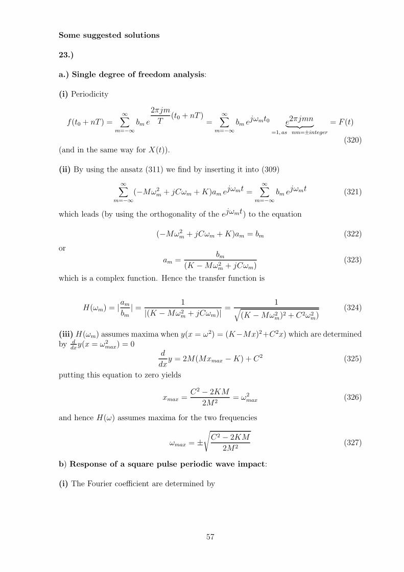
Some suggested solutions
23.)
a.) Single degree of freedom analysis:
(i) Periodicity
f(t0 + nT ) =∞∑
m=−∞
bm e
2πjm
T(t0 + nT )
=∞∑
m=−∞
bm ejωmt0 e2πjmn︸ ︷︷ ︸
=1, as nm=±integer
= F (t)
(320)(and in the same way for X(t)).
(ii) By using the ansatz (311) we find by inserting it into (309)
∞∑
m=−∞
(−Mω2m + jCωm +K)am ejωmt =
∞∑
m=−∞
bm ejωmt (321)
which leads (by using the orthogonality of the ejωmt) to the equation
(−Mω2m + jCωm +K)am = bm (322)
or
am =bm
(K −Mω2m + jCωm)
(323)
which is a complex function. Hence the transfer function is
H(ωm) = |ambm
| = 1
|(K −Mω2m + jCωm)|
=1
√
(K −Mω2m)
2 + C2ω2m)
(324)
(iii) H(ωm) assumes maxima when y(x = ω2) = (K−Mx)2+C2x) which are determinedby d
dxy(x = ω2
max) = 0d
dxy = 2M(Mxmax −K) + C2 (325)
putting this equation to zero yields
xmax =C2 − 2KM
2M2= ω2
max (326)
and hence H(ω) assumes maxima for the two frequencies
ωmax = ±√
C2 − 2KM
2M2(327)
b) Response of a square pulse periodic wave impact:
(i) The Fourier coefficient are determined by
57
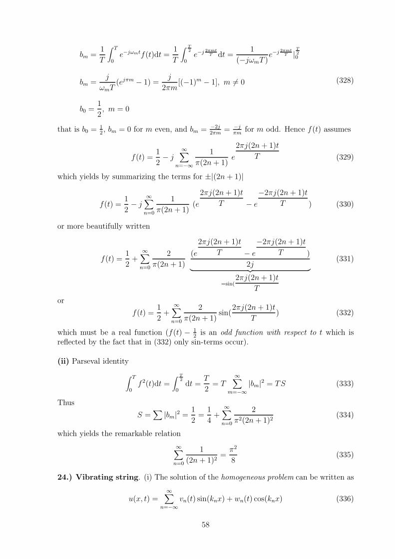
bm =1
T
∫ T
0e−jωmtf(t)dt =
1
T
∫ T2
0e−j 2πmt
T dt =1
(−jωmT )e−j 2πmt
T |T20
bm =j
ωmT(ejπm − 1) =
j
2πm[(−1)m − 1], m 6= 0
b0 =1
2, m = 0
(328)
that is b0 =12, bm = 0 for m even, and bm = −2j
2πm= −j
πmfor m odd. Hence f(t) assumes
f(t) =1
2− j
∞∑
n=−∞
1
π(2n+ 1)e
2πj(2n+ 1)t
T (329)
which yields by summarizing the terms for ±|(2n + 1)|
f(t) =1
2− j
∞∑
n=0
1
π(2n+ 1)(e
2πj(2n+ 1)t
T − e
−2πj(2n+ 1)t
T ) (330)
or more beautifully written
f(t) =1
2+
∞∑
n=0
2
π(2n+ 1)
(e
2πj(2n+ 1)t
T − e
−2πj(2n+ 1)t
T )
2j︸ ︷︷ ︸
=sin(2πj(2n+ 1)t
T
(331)
or
f(t) =1
2+
∞∑
n=0
2
π(2n+ 1)sin(
2πj(2n+ 1)t
T) (332)
which must be a real function (f(t) − 12is an odd function with respect to t which is
reflected by the fact that in (332) only sin-terms occur).
(ii) Parseval identity
∫ T
0f 2(t)dt =
∫ T2
0dt =
T
2= T
∞∑
m=−∞
|bm|2 = TS (333)
Thus
S =∑
|bm|2 =1
2=
1
4+
∞∑
n=0
2
π2(2n+ 1)2(334)
which yields the remarkable relation
∞∑
n=0
1
(2n + 1)2=
π2
8(335)
24.) Vibrating string. (i) The solution of the homogeneous problem can be written as
u(x, t) =∞∑
n=−∞
vn(t) sin(knx) + wn(t) cos(knx) (336)
58
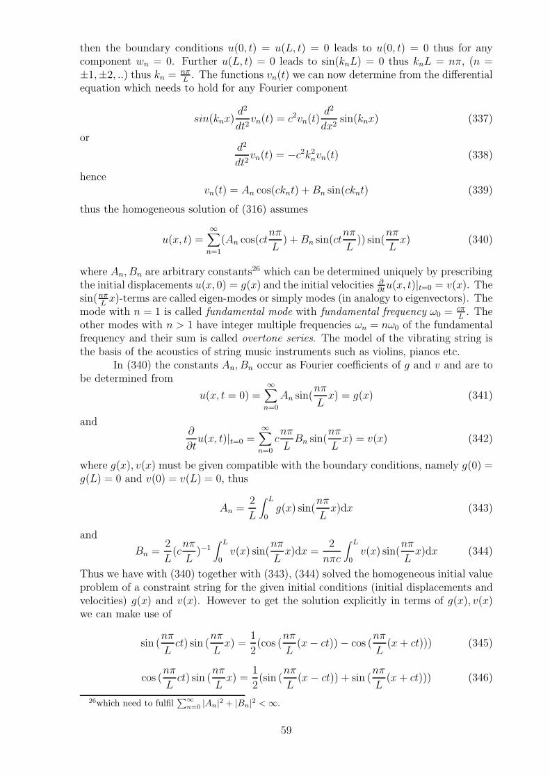
then the boundary conditions u(0, t) = u(L, t) = 0 leads to u(0, t) = 0 thus for anycomponent wn = 0. Further u(L, t) = 0 leads to sin(knL) = 0 thus knL = nπ, (n =±1,±2, ..) thus kn = nπ
L. The functions vn(t) we can now determine from the differential
equation which needs to hold for any Fourier component
sin(knx)d2
dt2vn(t) = c2vn(t)
d2
dx2sin(knx) (337)
ord2
dt2vn(t) = −c2k2
nvn(t) (338)
hencevn(t) = An cos(cknt) +Bn sin(cknt) (339)
thus the homogeneous solution of (316) assumes
u(x, t) =∞∑
n=1
(An cos(ctnπ
L) +Bn sin(ct
nπ
L)) sin(
nπ
Lx) (340)
where An, Bn are arbitrary constants26 which can be determined uniquely by prescribingthe initial displacements u(x, 0) = g(x) and the initial velocities ∂
∂tu(x, t)|t=0 = v(x). The
sin(nπLx)-terms are called eigen-modes or simply modes (in analogy to eigenvectors). The
mode with n = 1 is called fundamental mode with fundamental frequency ω0 =cπL. The
other modes with n > 1 have integer multiple frequencies ωn = nω0 of the fundamentalfrequency and their sum is called overtone series. The model of the vibrating string isthe basis of the acoustics of string music instruments such as violins, pianos etc.
In (340) the constants An, Bn occur as Fourier coefficients of g and v and are tobe determined from
u(x, t = 0) =∞∑
n=0
An sin(nπ
Lx) = g(x) (341)
and∂
∂tu(x, t)|t=0 =
∞∑
n=0
cnπ
LBn sin(
nπ
Lx) = v(x) (342)
where g(x), v(x) must be given compatible with the boundary conditions, namely g(0) =g(L) = 0 and v(0) = v(L) = 0, thus
An =2
L
∫ L
0g(x) sin(
nπ
Lx)dx (343)
and
Bn =2
L(cnπ
L)−1
∫ L
0v(x) sin(
nπ
Lx)dx =
2
nπc
∫ L
0v(x) sin(
nπ
Lx)dx (344)
Thus we have with (340) together with (343), (344) solved the homogeneous initial valueproblem of a constraint string for the given initial conditions (initial displacements andvelocities) g(x) and v(x). However to get the solution explicitly in terms of g(x), v(x)we can make use of
sin (nπ
Lct) sin (
nπ
Lx) =
1
2(cos (
nπ
L(x− ct))− cos (
nπ
L(x+ ct))) (345)
cos (nπ
Lct) sin (
nπ
Lx) =
1
2(sin (
nπ
L(x− ct)) + sin (
nπ
L(x+ ct))) (346)
26which need to fulfil∑
∞
n=0|An|2 + |Bn|2 < ∞.
59

Then we have for the first product sum in (340) with (341) with (346)
∞∑
n=1
An cos(ctnπ
L) sin(
nπ
Lx) =
1
2(g(x− ct) + g(x+ ct)) (347)
and for the second product sum in (340) with (342) and (345)
∞∑
n=1
Bn cos(ctnπ
L) sin(
nπ
Lx) =
1
2
∞∑
n=1
Bn(cos (nπ
L(x− ct))− cos (
nπ
L(x+ ct))) (348)
the last equation can be re-written by integrating (342)
1
2c
∫ x+ct
x−ctv(s)ds =
1
2c
∞∑
n=0
cnπ
LBn
∫ x+ct
x−ctsin(
nπ
Ls)ds (349)
With (347) and (349) we just have expressed the displacement u(x, t) of (340) interms of the given initial conditions u(x, 0) = g(x) and ∂u
∂t(x, 0) = v(x), namely
u(x, t) =1
2(g(x− ct) + g(x+ ct)) +
1
2c
∫ x+ct
x−ctv(s)ds (350)
Solution (350) is know in the literature as D’Alembert solution. It is easilyverified that the D’Alembert solution indeed solve the wave equation and fulfills the ini-tial conditions. The D’Alembert solution (350) applies not only for the vibrating string,generally solves Cauchy problems which are defined a homogeneous wave equation(316) together with the initial conditions (317).
60

4 Appendix
Here we give the proof for (108) which corresponds to the case that the set of n eigen-vectors are linear independent if the eigenvalues are all different to each other: To thisend we assume the set of eigenvalues {~vi} are linear dependent. Then the n×n-equationsystem
n∑
i=1
Ci~vi = V · ~C = 0 (351)
would have nontrivial (non-zero) solution-vector ~C = (Ci). Successive Multiplicationwith matrix A,A2, ..An−1 yields27, taking into account Ak~vi = λk
i ~vi
AkV · ~C =n∑
i=1
Ci~viλki = 0 (352)
where we generate n such equation systems (k = 0, .., n− 1). When we look at the pth
component of these n equation systems we obtain n equations of the form where (~vi)pdenotes the pth component of eigenvector ~vi
n∑
i=1
Ci~vipλki = P~
C = 0 (353)
with ~C = (Ci(vi)p)
P =
1, .., 1λ1, .., λn
..
λn−11 , .., λn−1
n
(354)
The determinant V = DetP is known as the Vandermond Determinant playingan important rule in many cases. In the questions (Question 13.)) we show that theVandermond determinant indeed is non-vanishing for λi 6= λj (i 6= j) and yields
V(λ1, λ2, .., λn) =
DetP = (λ2 − λ1)..(λn − λ1)(λ3 − λ2)..(λn − λ2)..(λn − λn−1)︸ ︷︷ ︸
n(n−1)2
factors
=∏
i<j
(λj − λi)
(355)Because of V(λ1, λ2, .., λn) 6= 0, i.e. the column vectors of P are linear inde-
pendent (because the λi 6= λj are all different) it follows that (352) has only the trivial
solution vector ~C = 0 and hence ~C = (Ci) = 0 which means that (351) has only the triv-ial solution. Hence the set of n eigenvectors ~v1, .., ~vn are indeed linear independent,which proves (108).
5 Literature
There is a vast amount of textbooks which cover the contents of this lecture. The two fol-lowing books are a suggested as they cover most of the contents of the lecture. There areplenty of other standard textbooks which cover this materials as well. Further reading
27Ak = A · .. ·A︸ ︷︷ ︸
k times
61

is explicitly encouraged (also in other than the below referenced textbooks). However,as the lecture does not strictly follow any textbook, these notes should be sufficient forthe comprehensive understanding of the topics addressed in this lecture.Part I:
[1] Glyn James (2004) Advanced Modern Engineering Mathematics, Pearson Education2004 (Third Edition).ISBN: 0 130 45425 7[2] Glynn James (2004) Modern Engineering Mathematics, Pierson Education.ISBN 0 130 45425 7 18319 9Part II:
[2] Bender, C. M.; Orszag, S. A., Advanced Mathematical Methods for Scientists andEngineers, New York: Springer, 1999ISBN 978-0-387-98931-0
62

6 Mock Exam
The following questions which comprise the complete module CIV6400 ”Mathematicsfor Dynamicists” are similar to those of previous exams. Answering of these questionsthus is highly recommended.
Question 1
(d2
dt2+ 2a
d
dt+ b2)X = f(t) (356)
for a, b ∈ R, b 6= 0, a > 0.1.) Give a fundamental solution system of the homogeneous problem (i.e. put f(t) = 0).
2.) Show by using the Wronskian determinant that the system of solutions of thehomogeneous problem you gave in 1.) indeed is a fundamental system.
3.) Determine the general solution X(t) for f(t) = eαt for α2 + 2aα + b2 6= 0.
4.) Solve the initial value problem
(d2
dt2+ 2a
d
dt+ b2)X = 2 cos t (357)
with initial conditionsX(t = 0) = A0,dXdt(t = 0) = A1.
Hint: make use of 2 cos t = eit + e−it, i =√−1 by using:
(i) Operator method(ii) Laplace transformation
5.) Consider now (356) for α = iω, i.e. a driving external force f(t) = eiωt whereω ∈ R is the frequency of this force. Determine for this case the so called enhancementfactor V which is defined by
V =: limt→∞
|xp(t)||f(t)| (358)
where xp(t) denotes any particular solution of the non-homogeneous problem. For thislimiting case which leads to the ’steady state’ solution the fact that a > 0 (which guar-antees exponential damping of the homogeneous solution) is important.
(i) Why is definition (358) unique, i.e. independent of given initial conditions?
(ii) For which values of the exciting frequency ω the enhancement factor V takes amaximum?
(iii) Determine the maximum value of V .
(iv) Sketch V (ω) vs ω schematically.
63
6.) Determine the so referred to as phase shift of the solution 3.) which is definedby
φ =: limt→∞
{arg(Xp(t))− arg(f(t))} = limt→∞
arg[Xp(t)
f(t)] (359)
Question 2Given the recursion
Xn+1 = aXn + bYn; Yn+1 = bXn + aYn; n = 0, 1, 2, .. (360)
initial values X0 = 2, Y0 = 1. Hint: It is convenient to consider the given recursion inmatrix form, i.e. ~xn+1 = M~xn with start vector ~x0.1.) Determine ~xn = (Xn, Yn) in dependence of ~x0 = (X0, Y0).2.) Determine the limiting case A = limn→∞(Xn
Yn) for b > 0.
(i) Does the result depend on c for initial conditions X0 = c, Y0 = c?
3.) Consider now the modified recursion
Xn+1 = α(aXn + bYn); Yn+1 = α(bXn + aYn);n = 0, 1, 2, .. (361)
for a > b > 0.
(i) For which values α > 0 exist the sums Sx =∑∞
n=0Xn, Sy =∑∞
n=0 Yn? Hint: Reducethe problem to the consideration of geometrical series of the form
∑∞n=0[α(a± b)]n and
consider for what values of α > 0 this series is convergent.
(ii) In the case of convergence, determine the values of these sums for the initial condi-tion (X0 = 1, Y0 = −1).
Question 3Given the recursion
Xn+1 = Xnρ cosϕ− Ynρ sinϕ; Yn+1 = Xnρ sinϕ+ Ynρ cosϕ;n = 0, 1, 2, .. (362)
with ϕ ∈ R and ρ ∈ R with initial conditions X0 = A, Y0 = B. For which ρ hold
(i) limn→∞X2n + Y 2
n = 0?
(ii) limn→∞X2n + Y 2
n = A2 +B2?
(iii) limn→∞X2n + Y 2
n = ∞?
Question 4
Determine the solution for the initial value problem (D = ddt)
P (D)X = e−3t; P (D) = D2 + 6D + 9 (363)
with initial conditions X(t = 0) = 1, ddtX(t = 0) = 0 by using
(i) Operator method(ii) Laplace transformation
64
Question 5
Given the differential equation L[u] = f(t) where L[u] = u′′ − 6u
′
+ 25u.
a) Determine the general solution uh(t) of the homogeneous differential equation (f(t) =0).
b) Determine that special solution (particular integral) up(t) for f(t) = eiωt which isperiodic.
c) Determine the frequency of resonance, i.e. the frequency ωr for which |up| is a maxi-mum.
d) Determine the times τn > 0 when the periodic solution up(t) is purely real?
e) Determine the special solution of the non-homogeneous differential equation forf(t) = eiωt which fulfills the initial conditionsu(t = 0) = A
u′
(t = 0) = B
Question 6Given the differential equation L[u] = f(t) whereL[u] = u
′′′ − 3u′′
λ+ 3u′λ2 − λ3.
a) Determine the special solution (complementary function) uh(t) of the homogeneousdifferential equation (f(t) = 0) which fulfills the conditionsu(t = 0) = A
u′
(t = 0) = 0u
′′
(t = 0) = 0b) For which value of A holds uh(1) = e?
c) Determine a particular solution up(t) for f(t) = ebt
(i) for b 6= λ
(ii) for the case b = λ
d) Consider now the case b = λ, i.e. f(t) = eλt:(i) Give the general solution u(t) = uh(t) + up(t).
Question 7
Given the set of functions: X1 = e−t, X2 = et, X3 = e(2+i)t, X4 = e(2−i)t.Determine the homogeneous differential equation P (D)X(t) = 0 from which this set offunctions constitutes a fundamental system.
65