mass spectrum labeling: theory and practiceresearch.cs.wisc.edu/edam/spectrumtr.pdf · mass...

University of Wisconsin – Madison Technical Report

- 1 -

Mass Spectrum Labeling: Theory and Practice

Zheng Huang, Lei Chen

Jin-Yi Cai, Deborah Gross*, Raghu Ramakrishnan, James J. Schauer*, Stephen J. Wright

Computer Sciences Department, University of Wisconsin-Madison

ABSTRACT

In recent years, a number of instruments have been developed for continuous,

real-time monitoring of the environment. Aerosol mass spectrometers can analyze

several hundred atmospheric aerosol particles per minute and generate a plot of

mass-to-charge versus intensity (a mass spectrum) for each particle. The mass

spectrum could be used to identify the compounds present in the particle in real-

time, in contrast to conventional filter-based approaches in which filters collect

samples over a period of time and are then analyzed in a laboratory, but our ability

to analyze the data is currently a bottle-neck. In this paper, we introduce the

problem of labeling a particle’s mass spectrum with the substances it contains, and

develop several formal representations of the problem, taking into account practical

complications such as unknowns and noise.

Our contributions include the introduction and formalization of a novel data

mining problem, theoretical characterizations of the central difficulty underlying

the problem, algorithms for solving the problem, metrics to measure the quality of

labeling, experimental evaluation of the effectiveness of these algorithms, and

comparisons with alternative machine learning techniques (showing that our

algorithms, although slower, achieve uniformly superior accuracy without the need

for training datasets!).

1. INTRODUCTION

Mass spectrometry techniques are widely used in many disciplines of science, engineering, and biology for the

identification and quantification of elements, chemicals and biological materials. Historically, the specificity of

mass spectrometry has been aided by upstream separation to remove mass spectral interference between different

species. Examples include gas- (GCMS) and liquid-chromatography mass spectrometry (LCMS), and off-line

wet chemistry clean-up techniques often employed upstream of inductively coupled plasma mass spectrometry


- 2 -

(ICPMS). Historically, these techniques have been employed in laboratory settings that did not require real-time

data collection, and the time required for separation and clean-up has been acceptable.

In the past decade, a wide range of real-time mass spectrometry instruments have been employed, and the

nature of these instruments often precludes separation and clean-up steps. The mass spectrum produced for a

particle in real-time by one of these instruments is therefore comprised of overlaid mass spectra from several

substances, and the overlap between these spectra makes it difficult to identify the underlying substances. The

Aerosol Time-of-Flight Mass Spectrometer (ATOFMS) [11,9,13,15] is an example that is currently available

commercially, and is used to monitor the size-resolved chemical composition of airborne particles. This

instrument can obtain mass spectra for up to about 250 particles per minute, producing a time-series of unusual

complexity. We have applied our results to ATOFMS data, although the data analysis challenges we describe are

equally applicable to other real-time instruments that utilize mass spectrometry.

Unlabeled Spectrum:

Labeled Spectrum:

Na+

Al+

Fe+Ca+

FeO+K2Cl+

Fe2O+

Ba+ BaO+

BaFeO+

BaFeO2+

BaFe+BaCl+

0 100 300200m/z

Na+

Al+

Fe+Ca+

FeO+K2Cl+

Fe2O+

Ba+ BaO+

BaFeO+

BaFeO2+

BaFe+BaCl+

0 100 300200m/z

0 100 3002000 100 300200m/z

Figure 1: Mass Spectrum Labeling

Mass spectrum labeling consists of “translating” the raw plot of intensity versus mass-to-charge (m/z) value to

a list of chemical substances or ions and their rough quantities (omitted in Figure 1) present in the particle.

Labeling spectra allows us to think of a stream of mass spectra as a time-series of observations, one per collected

particle, where each observation is a set of labels (or ion-quantity pairs). This is similar to a time-series of

transactions, each recording the items purchased by a customer in a single visit to a store [1,4,13]. This analogy

makes a wide range of association rule [3] and sequential pattern algorithms [2] applicable to the analysis of

labeled mass spectrometry data.

The contributions of this paper include:

• In this and a companion paper [7], we introduce a new and important class of data mining problems

involving analysis of mass spectra. The focus in this paper is on the labeling of individual spectra (Section

2), which is the foundation of a class of group-oriented labeling tasks discussed in [7]. Labeling also allows

us to view spectra abstractly as “customer transactions” and borrow analysis techniques such as frequent

itemsets and association rules. There is also a deeper connection to market-basket analysis in that our

formulation of labeling allows us to search for buying patterns of interest (“phenomena” [10]) rather than

just sets of items frequently purchased together [7].


- 3 -

• We present a theoretical characterization of ambiguity, which arises because of the presence of substances

whose individual spectra overlap in the given input spectrum, and controls whether or not there is a unique

way to label the input spectrum. (Section 3)

• We extend the labeling framework to account for practical complexities such as noise, errors, and the

presence of unknown substances (Section 4). We then present two algorithms for labeling a spectrum, using

this realistic problem formulation, together with several optimizations and results characterizing their

behavior. (Section 5).

• A major difficulty for researchers is the effort involved in generating accurately labeled “ground truth”

datasets. Such datasets are invaluable for training machine learning algorithms, tuning algorithms for a

given application context using domain knowledge, and for comparing different algorithms. We present a

detailed synthetic data generator that is based on real mass spectra, conforms to realistic problem scenarios,

and allows us to produce labeled spectra while controlling several fundamental parameters such as ambiguity

and noise. (Section 6).

• Finally, we discuss and rigorously define a metric for measuring the quality of labeling, and present a

thorough evaluation of our labeling algorithm and a comparison with machine learning approaches, showing

that our algorithms, although slower, achieve uniformly superior accuracy without the need for training

datasets! (Section 7)

Related work and future directions are discussed in Section 8.

2. PROBLEM FORMULATION

A mass spectrum (or spectrum) is a vector 1 2[ , ]rb b b b= , where ib R∈ is the signal intensity at mass-to-charge

(m/z) value i. For simplicity, we assume all spectra have the same ‘range’ and ‘granularity’ over the m/z axis; i.e.,

they have the same dimension r and the ith element of a spectrum always corresponds to the same m/z value i.

Intuitively, each m/z ratio corresponds to a particular isotope of some chemical element. The signature of an ion

is a vector 1 2[ , ]rs I I I= , iI R∈ and ∑ =i iI 1 , representing a distribution of isotopes, i.e., iI is the proportion of the

isotope with m/z value i. A signature library is a set of known signatures 1 2{ , }nS s s s= , in which js is the

signature of ion j. Additionally, there may be ions that appear on particles, and are therefore reflected in mass

spectra, but that for which signatures are not included in the signature library.

The spectrum b of a particle is a linear combination of the signatures of ions that it contains, i.e., ∑= j jj swb ,

where jw is the quantity of ion j in the particle. The task of mass spectrum labeling is to find the quantities wj of

all ions present in the particle, given an input spectrum. Formally, a label for an ion with respect to a given

spectrum is an <ion, quantity> pair; a label for the spectrum is the collection of labels for all ions in the signature


- 4 -

library. The task of labeling an input spectrum can be viewed as a search for a linear combination of ions that

best approximates the spectrum, and the success that is achievable depends on the extent of unknown ions. When

developing our algorithms, in Sections 3 to 5, for simplicity we assume that the signature library is complete, i.e.,

there are no unknown ions. We evaluate the impact of unknowns in Sections 6 and 7.

3. WHEN IS LABELING HARD?

In this section, we formulate the labeling task as solving a set of linear equations, and then discuss the

fundamental challenge involved: interference between different combinations of signatures and the consequent

ambiguity in labeling.

3.1 Linear System Abstraction

We can represent the signature library 1 2{ , }nS s s s= as a matrix ] ,...,,[ 21 nsssA = , where ks , the kth column of A, is

the signature of ion k. A spectrum label is an n-dimensional vector x whose jth component [ ]x j indicates the

quantity of ion j in the particle. Labeling consists of solving the linear system Ax b= , 0x ≥ . Noticing

that Ax b= ( ) ( )A x bα α⇒ = for any constant α , we can assume without loss of generality that b is normalized

(i.e., 1][ =∑i ib ). By definition of signatures, each column of A also sums to 1. It follows immediately from this

fact and ∑ =i ib 1][ that ∑ =i ix 1][ . The exact quantity of all ions can be easily calculated by multiplying the quantity

distribution vector x by the overall quantity of the particle, which is simply the sum of signal intensities over all

m/z values in the original spectrum before normalization.

3.2 Uniqueness

In general, given the signature library A and an input spectrum b , neither existence nor uniqueness of

solutions for the system

Ax b= , 0x ≥ (1)

is guaranteed. We define following important property.

Definition 1: An input spectrum b is said to have the unique labeling property with respect to signature library A

if there exists a unique solution 0x to the system Ax b= , 0x ≥ .

For an important class of libraries, we have the following result.

Theorem 1: Consider signature library ] ,...,,[ 21 nsssA = and a spectrum b where nsss ,...,, 21 are linearly independent

(i.e., there is no vector a = 1 2[ , ,..., ]na a a such that ∑ =ni ii sa1 and at least one 0ia ≠ ). Then, either b has the unique

labeling property w.r.t. A, or the system of equations (1) has no solution.

[Proof: See Appendix A]


- 5 -

Even if a signature library does not satisfy the conditions of Theorem 1, there may still be input spectra b for

which the solution of (1) is unique. For example, when

( )10 1 1 / 2,

01 0 1 / 2A b= =⎛ ⎞⎜ ⎟

⎝ ⎠

there is a unique solution [0,1,0]Tx = .

Conversely, there will typically be infinitely many solutions for a given spectrum when the signature library

does not satisfy the conditions of Theorem 1. For example, let there be a nonzero vector

a = 1 2[ , ,..., ]na a a with 0=aA , and equation (1) has a solution 1 2[ , ,..., ]nx x x x= with 0,...,2,1 >= ini xmin . Then xa +β is a

solution to (1) for all β with sufficiently small magnitude.

Theorem 2: Consider signature library ] ,...,,[ 21 nsssA = and a spectrum b where nsss ,...,, 21 are not linearly

independent. If there is a solution ],...,,[ 21 naaaa = to Ax b= , 0x ≥ such that 0,...,2,1 >= ini amin , then b has infinitely

many labels.

[Proof: See Appendix B]

3.3 Spectra with Unique Labeling

In this section, we characterize the complete set of spectra that have the unique labeling property with respect

to a given signature library. We explain the concept by means of a pictorial example and then state a theorem that

describes this set.

Suppose the signature library has only four signatures 4321 ,,, ssss . Figure 2(a) shows the case in which 421 ,, sss

are linearly dependent. All normalized spectra that can be represented as a conic combination (that is, a linear

combination of the vectors 4321 ,,, ssss in which the coefficients are nonnegative) form the triangle 321 sss∆ in this

example. The ambiguity of the labeling comes from the linear dependency among 421 ,, sss , since 4s is itself a conic

combination of 1s and 2s . However, any point lying on the line 31ss can be uniquely represented as a conic

combination of 1s and 3s . The intuitive reason for this is clear: Any involvement of a positive fraction of 2s or 4s

(or both) will lift the point out of the line 31ss . Similarly the points on the line 32ss can be uniquely represented as

a conic combination of 2s and 4s . The case in which 4s combines all three vectors, 321 ,, sss is shown in Figure 2(b).

In this case, any point lying on the boundary of triangle 321 sss∆ can be uniquely represented as a conic

combination of two signatures among 321 ,, sss .

We now characterize the tight boundary of spectra with unique labeling property formally. A polynomial time

algorithm for testing the unique labeling property of a spectrum is also presented in Appendix C.


- 6 -

Definition 2: Given a signature library 1 2{ , }nS s s s= , the convex hull generated by S is defined as:

}1,,0,1,1|{)( 11 niSswwnswSch iini i

ni ii ≤≤∈≥=≥= ∑∑ ==

Theorem 3: The set of spectra with the unique labeling property w.r.t. library S is the set of points in ch(S) that

do not lie in the interior of the convex span of some affine dependent subset of S.

[Proof: See Appendix D]

4. HANDLING AMBIGUITY AND ERRORS

In practice, signal intensities are not precisely calibrated, and background noise causes measurement errors and

introduces uncertainty. We therefore introduce an error bound E and a distance function D, and recast the labeling

problem in terms of mathematical programming, as an “exhaustive” feasibility task:

Seek all such that ( , ) , 0.a D Aa b E a≤ ≥ (2)

(a)

(b)

Figure 2: Vector Space Spanned by Signatures

Given a library A with n signatures and input spectrum b , the search space for problem (2) is a n-

dimensional1 space. The solution space for input spectrum b is defined as follows.

Definition 3 : Given a signature library A, an input spectrum b and an error bound E with respect to distance

function D, the solution space of spectrum b is { }| ( , ) , 0 .L a D Aa b E ab= ≤ ≥

It is worth noting that the choice of the distance function D may affect the complexity of the problem

significantly. We use Manhattan Distance (also known as 1 norm), which allows us to find a specific element of

the solution set for (2) by using the following linear programming (LP) model:

. . , , 0, 0.iimin s s t Aa b s Aa b s a s− ≤ − ≥ − ≥ ≥∑

We observe that if the distance function is convex, the solution space of an input spectrum b is convex (see

below). We will explore this property further in Section 5; for now, we note that Manhattan Distance is a convex

distance function.

1 Actually, an n-1 dimensional space if b is normalized.


- 7 -

Theorem 4: If the distance function D has the form ( , ) ( ),D u v d u v= − where d is a convex function, then the

solution space of the search described by Equation (2) is convex.

Proof: Let 1a and 2a be two elements of the solution space. We wish to show that 21 )1( aaa αα −+= is also a

member of the solution space, for any [0,1]α ∈ . Since 1 0a ≥ and 2 0a ≥ , we have trivially that 0a ≥ also. In addition,

by definition of a and convexity of d , we have

( ) ( )( ) ( )

1 2

1 2

( , ) ( ) (1 )( )

(1 ) (1 ) ,

D Aa b d Aa b d Aa b Aa b

d Aa b d Aa b E E E

α α

α α α α

= − = − + − −

≤ − + − − ≤ + − =

so that EbaAD ≤),( and a is a member of the solution space.

4.1 Discretization

Even if an input spectrum has an infinite number of labels (for a given signature library) because of ambiguity,

in practice, we do not need to distinguish between solutions that are very similar. A natural approach to deal with

the infinity in a continuous space is to discretize it into grids, so that the number of possible solutions becomes

finite.

Formally, a threshold vector ],...,,[ 10 dtttt = divides each dimension of the search space into d ranges, where it

and 1it + are the lower bound and upper bound of range i. Given a threshold vector, we introduce the notion of

index vector to represent a continuous subspace.

Definition 4: Given a threshold vector ],...,,[ 10 dtttt = , an index vector 1 1 2 2[( , ),( , ),...,( , )], , ,n n i i i iI l h l h l h l h l h Z= < ∈

represents a continuous subspace,

}][],[][][,|{ RiaihtiailtiaSI ∈≤<∀=

Since an index vector represents a unique subspace, we will refer to a subspace simply by its corresponding

index vector when the context is clear. Using the index vector representation, we in turn define the notion of cell.

Definition 5: A subspace 1 1 2 2[( , ),( , ),...,( , )]n nl h l h l h is a cell if , 1j jj l h∀ + = .

The cell is the finest granularity of the discretization, which reflects the degree of detail users care about. A

threshold vector ],...,,[ 10 dtttt = divides the whole search space into nd cells, where n is the number of dimensions

(which is equivalent to the total number of signatures in the signature library). Each cell also corresponds to a

distinct n-dimensional integer vector

Zydyyyyy iin ∈≤≤= ,1],,...,,[ 21

which defines a subspace Y corresponding to the index vector )]1,(),...,1,(),1,[( 2211 +++ nn yyyyyy .


- 8 -

4.2 Optimization Model

We now redefine the task of spectrum labeling as follows: Find all the cells that intersect the solution space

of the input spectrum. A label of spectrum b is then simply an integer vector x whose cell intersects the solution

space corresponding to b . All integer vectors whose corresponding cells intersect b 's solution space form the label

set of spectrum b . Formally,

Definition 6: x is a label of spectrum b if the subspace defined by the index vector

1 1 2 2[( , 1),( , 1),..., ( , 1)]n nX x x x x x x= + + + intersects the solution space of spectrum b . Spectrum b 's label set

is { | is a label of }L x x b=

To simplify the discussions in the following sections, we also introduce the notion of feasible space to

describe a subspace that intersects the solution space of the input spectrum. If the feasible space is a cell, it is also

called label, because there is a one-one correspondence between a label and a cell that intersects the input

spectrum's solution space.

Figure 3 illustrates the concepts discussed in this section. Suppose there are only two signatures in the

signature library. The whole search space is a two dimensional space ABCD within which 1 2 3 4S S S S forms the

solution space of a input spectrum. It intersects the cells LFGM and MGHA, each of which corresponds to a label.

Subspace ALFH intersects with the solution space, so it is a feasible space. MBEG is also a feasible space.

Table 1 summarizes our notation and describes an optimization model for the labeling task.

Notations: x An n-dimensional integer vector, 1 [ ]x i d≤ ≤

b Normalized input mass spectrum

t Threshold vector for discretization

d Number of ranges per dimension under the discretization

L Label set of input spectrum

A Signature library with n signatures

D Distance function

E Error bound

L = ∅

for every possible x

s.t.

D(Aa, )

t[ ] [ ] [ 1], [ ] (*)

if (*) succeeds, { }

Seek a

b E

j a i t j j x i

L L x

≤

< ≤ + =

= ∪


- 9 -

return L

Table 1: Operational Definition of Spectrum Labeling

5. LABELING ALGORITHMS

In Section 4, we showed that given n signatures and discretization granularity d, the search space contains nd

cells. A brute force approach that tests the feasibility of each cell is not practical, considering that there are

hundreds of signatures. In this section, we propose two algorithms: DFS is general, and Crawling exploits

convexity of distance functions.

Figure 3: Illustration of Concepts

5.1 Feasibility Test

Given a subspace S, we use the algorithm shown in Table 2 to test the feasibility of the subspace; this algorithm is

a building block. Notice that exactly one LP call is invoked for the test.

5.2 Depth-First Search (DFS) Algorithm

Before we specify the DFS algorithm, we first state an important property of subspace feasibility. The proof is

straightforward and is omitted.

Theorem 5: Let a spectrum b and a signature library A with n signatures be given. If subspace S is feasible, then

any subspace T , with S T⊂ is also feasible.

The DFS labeling algorithm explores a search tree in which each node is associated with a particular subspace,

and the subtree rooted at that node corresponds to the subsets of that subspace. At each node, the algorithm first


- 10 -

tests the feasibility of the subspace for that node. If not feasible, that node and its subtree are pruned. Otherwise,

we select a dimension j that has not been subdivided to the finest possible granularity in the subspace of that node,

and divide the subspace further along dimension j. Each smaller space created thus corresponds to a child of the

current node.

In Table 3, the pick_dimension method chooses a dimension (which is not already at the finest granularity

possible) to split the current subspace, and split_subspace divides the current subspace into smaller pieces along

the chosen dimension. Variants of these two methods are discussed in the following subsections.

Input: b Input mass spectrum

E Error bound

t Threshold vector

Output: TRUE if the subspace is feasible, FALSE

otherwise

Is_feasible(subspace S)

1 1 2 2

s.t.

( , ) (*)

t[ ] [ ] [ ], for 1,2,...,

[( , ),( , ),...,( , )] is the index vector of subspace if (*) succee

j j

n n

Seek a

D Aa b E

l a j t h j n

l h l h l h S

≤

< ≤ =

ds, return TRUE, otherwise return FALSE

Table 2: Test The Feasibility of A Subspace


E Error bound t Threshold vector

Output: Label set )(bL

Depth_First_Search(subspace S)

∅←L

if not Is_feasible(S) return L; else if S is a cell L ← label corresponding to S;

return L; else pick_dimension(j)

{ }iS = split_subspace(S, j)


- 11 -

for each iS

←L L ∪ Depth_First_Search( iS )

return L;

Main : Depth_First_Search(whole search space W)

Table 3: Depth First Search Algorithm

5.2.1 Split Subspace

After the split dimension is chosen, the current subspace will be divided along the chosen dimension into

smaller slices. Suppose the index vector corresponding to the current subspace is )],(),...,,(),,[( 2211 nn hlhlhlI = and the

split dimension is j, the simple split variant will divide the subspace into “slices”, each of which has the finest

granularity in dimension j. That is, the resulting “slices” to be explored individually at the next level of recursion

are { )],(),...,1,(),...,,[( 11 nn hlxxhl + | 1j jl x h≤ ≤ − }. The binary split variant divides the subspace into two “slices” of

approximately equal width along dimension j. If a particular dimension, which corresponds to a signature in the

library, has various values across different labels, the simple split scheme is better than the binary split scheme. If

a convex distance function is used, we can even adopt a binary search strategy to determine the boundary of the

spectrum’s solution space and split the dimension in a way that only one of the resulting “slices” intersect with the

spectrum’s solution space. Our implementation of the DFS algorithm does not rely on the convexity of the

distance function. The simple split scheme is used.

5.2.2 Pick Dimension

The choice of dimension along which to split affects the efficiency of the DFS algorithm in practice. Suppose

we have two signatures in the library and the labels for the given input spectrum are [0,1] (cell LFGM) and [0,2]

(cell MGHA), as illustrated in Figure 3. The simple split scheme is used. Figure 4(a) shows the search tree when

we first choose dimension 1 (x-axis). It divides the whole search space into three slices BEHA, EVUH and VCDU

and tests the feasibility of each. BEHA is a feasible subspace and is further split on dimension 2. Cells BEFL,

LFGM, MGHA are tested. Two labels LFGM and MGHA are found and the algorithm terminates. Similarly,

Figure 4(b) shows the case when dimension 2 is selected first. In this case, the search space is first split along the

y-axis, resulting in two feasible subspaces LQPM and MPDA for further exploration. In the search trees shown in

Figure 4, each node corresponds to a subspace upon which an LP call is invoked. A node is colored black if it

corresponds to a feasible subspace. Leaf nodes correspond to cells in the discretized search space. A leaf node is

black if it corresponds to a label. As we can see, the first search tree invokes 7 LP calls and the second one

invokes 10 LP calls. When the tree is large, the performance difference between various pick_dimension schemes

becomes even more significant. Generally speaking, during the search process, we would like to select those

dimensions (signatures) which lead to fewer future splits. A “greedy” algorithm would select the split node to be

the one that has the fewest feasible children. If all labels have the same value on a particular dimension (that is,

just one feasible child), that dimension is ‘good’ and should be selected as early as possible.


- 12 -

Theorem 6 shows that if a convex distance function is used and the number of labels for the input spectrum is

at most equivalent to the number of signatures in the signature library, the existence of such a “good” dimension

is guaranteed. In our current implementation of the DFS algorithm, we simply choose a dimension that has not

been selected before.

1

2

2

1

(a) (b)

dimensionselected

dimensionselected

BCDA

BEHA

LFGM MGHA

BCDA

LQPM MPDA

LFGM MGHA

Figure 4. Search Trees for Different Split Dimension Choices

Theorem 6: Suppose the convex set K is contained in some “brick” ],[...],[ 11 nn ULULB ××= and that B is divided

into ir ranges along each dimension i , iriiii UaaaLi=<<= ,2,0, , and B is the union of∏ =

ni ir1 many “sub-bricks” of the

form ],[...],[ 1,,1,1,1 11 ++ ××nn jnjnjj aaaa . If K has nonempty intersection with at most n of these “subbricks”, then there

exists a dimension i, and a “slice” ]},[|{ 1,, +∈∈ii jijii aaxBx that contains K.

[Proof: See Appendix E]

5.2.3 Correctness and Complexity

Theorem 7: Given an input spectrum and a specified error bound, the DFS algorithm finds the complete label set

of the spectrum.

Proof: The algorithm checks the feasibility of nodes from top to bottom of the search tree. Each child of a node

will be visited if that node represents a feasible solution subspace. Each label corresponds to a feasible cell and,

according to Theorem 5, all its supersets will also be feasible. Hence there is a path from the root search node to

each label node, such that all the nodes along this path correspond to feasible subspaces and therefore will not be

pruned. Because of this fact, the search node for each label will be visited eventually and the label will be output.

On the other hand, every output label corresponds to a cell. The is_feasible test on that cell guarantees that it is

output as a label for the spectrum only if it is feasible.

It can be shown that given a signature library with n signatures and a threshold vector that divides each

dimension into d ranges, the number of LP calls invoked by DFS algorithm to label a spectrum with k labels is

O(knd). A detailed analysis based on a “node coloring” model is presented in [7].


- 13 -

5.3 The Crawling Algorithm

DFS is a general algorithm in which we can use any distance function D, even one that is non-convex. The

Crawling algorithm requires the distance function to be convex and exploits the connectivity property2 derived

from the convexity of solution spaces, as described in Theorem 5.

Connectivity Property: Given two labels l1 and ln, there exists a path of connecting labels ( l1 ,…, li-1 , li ,… ln ) in

which li-1 , li are adjacent, i.e., differ only in one dimension by 1.


E The error bound t The threshold vector

Output: Label set of b

Crawling() aSeek s.t. 0][,),( ≥≤ iaEbaAD (*)

if (*) fails return ∅ else ∅←L find 0 1 2[ , ,..., ]nl x x x= s.t. ]1[][][ +≤< ii xtiaxt , 1,2,3,...,i n= insert l0 into the queue Q and mark l as generated while (Q is not empty) { pick the first index vector ],...,,[ 21 nxxxl = from Q }{lLL ∪← and remove l from Q for j = 1 to n do if ( 1−≠ dxi ) ],...,1,...,,[' 21 nj xxxxl +=

if 'l is a label of b and 'l has not been generated before, then

insert 'l into Q , mark l’ as generated if 0≠ix ],...,1,...,,[" 21 nj xxxxl −=

if ''l is a label of spectrum b and ''l has not be generated before, then insert ''l into Q, mark ''l as generated } // end of while loop return L

Table 4: Crawling Algorithm

The Crawling algorithm first finds a solution to the linear system 0][,),( ≥≤ iaEbaAD by invoking a LP call. The

cell contains that solution is a label and is used as the start point to explore other connected cells in a breath-first

fashion. If the cell discovered has not been visited before and is a label, its neighbors will be explored

2 Convexity is actually stronger than the connectivity property.


- 14 -

subsequently. Otherwise, it is discarded and no further exploration will be incurred by it. The algorithm stops

when all labels and their neighbors are visited. The connectivity property guarantees that all labels are connected

to the first label we found and can be discovered by “crawling” from that start point. The algorithm is described in

Table 4.

Let’s take Figure 3 in Section 4 again as an example. The input spectrum’s label set contains two labels which

are the cells in shade. The crawling algorithm first finds a solution point. Suppose it falls in cell LFGM. It then

starts from LFGM and explores its neighbors LBEF, FROG and MGHA. Among the three, only cell MGHA is a

label and will incur further exploration. It has only two adjacent cells. One is already visited and the other is not a

label. Thereby the algorithm terminates and outputs LFGM and MGHA as the input spectrum’s label set.

Theorem 8 Given an input spectrum b , a signature database 1 2[ , ,..., ]nA S S S= and a threshold vector 1 2 1[ , ,..., ]dt t t t += ,

suppose the number of labels for b is k, the Crawling algorithm will find the complete set of the labels for input

spectrum.

Proof:

Completeness: According to the connectivity property, any label l connects to the initial found label l0, i.e., there

is a label path 1, ,..., ,o x xnl l l l . Along this path, 1xl will be found when 0l is removed from the queue Q and all the

neighbors of 0l are tested. 2xl will be found at least when 1xl is picked and its neighbors tested. (Note that 2xl does

not necessarily to be generated from 1xl since there might be other path which lead from 0l to 2xl ). By using

induction, it is easy to see that l will be found not later than the time when xnl is picked and its neighbor tested.

Hence, All the labels will finally be collected in queue Q and put in the result set L .

Correctness: All the labels found by Crawling algorithm are correct because one index vector has to go through

the feasibility test before it is inserted into the queue Q. The result label set L only contains labels come from Q.

Hence, all the labels in L should be correct.

Theorem 9: Given an input spectrum b , a signature library ] ,...,,[ 21 nsssA = and a threshold vector ],...,,[ 10 dtttt = ,

suppose the number of labels for b is k, then the number of LP calls invoked by the Crawling algorithm is O(kn).

The number of index vectors stored in the queue is O(kn).

Proof: Each cell in the grid has at most 2n neighbors, two in each dimension. We paint all the cells in the grid

using the following rules: 1) If a cell is a label, we paint it black; 2) if a cell is not a label, but it has a label

neighbor, we paint it grey; 3) if a cell neither is a label nor has a label neighbor, we paint it white. The number of

black cells equals to the number of labels k. Since each cell has at most 2n neighbors and there are k black cells,

the number of grey cells is at most 2kn. According to the connectivity property, all black cells are connected to

each other by a path consisting of only black cells. The algorithm will only generate those cells in black or grey


- 15 -

and invoke exactly one LP call for each of them. Since the number of black and grey cells together is no more

than k+2kn, the number of LP calls invoked is O(kn)

The number of index vectors in the queue Q equals to the number of black cells and grey cells. As stated

above, the number of black and grey cells is O(kn).So the space complexity of the crawling algorithm, which is

measured by the number of index vectors in the queue, is also O(kn).

5.4 Directional Bounding Algorithm

We now describe an algorithm that is similar to crawling in that it progressively identifies solutions by

searching in different dimensions successively. The approach differs in that it uses a binary search to determine

the extent of the solution space along a given dimension. Hence, it may not need to actually solve a linear

program for each of the cells that actually solve (2). For solutions sets with certain shapes that extend over a

moderate to large number of cells, and for moderate to large values of ,d this approach may yield significant

savings over the Crawling Algorithm and DFS.

In order to specify the directional bounding (DB) algorithm and the binary search at its core, we first define

some notation:

( ){ }

( ) { } [ ] [ ] [ ]( ) { }

{ }

1

label Label set of

1,2,..., "explored" dimensionsinteger in 1,2,...,d such that

ˆ set of elements , where 1,2,... , 1,2,... , and 1,2,..., .

i i i i

i

b b

D nx a x t x a i t x

Q x D x d i nD n

+

=

⊂ =

= ≤ <

= ∈ =

⊂

The binary search procedure in Table 5 picks a certain cell x belonging to ( )label b and explores a given

dimension k. to see how far the label set extends along this dimension.

Input: Spectrum b , threshold vector [ ]1 2 1, ,..., ,dt t t t +=

error bound E , label label( )x b∈ , search dimension k .

Output: labels ( , )l r with 1 l r d≤ ≤ ≤ .

( , )l r ← BinarySearch ( ),x k

1, ;U kr d r x← + ←

while 1Ur r− >

( ) / 2Up r r= +⎢ ⎥⎣ ⎦ ;


- 16 -

if there exists a such that

[ ] [ ] [ ][ ] [ ] [ ]

1

( , ) , 0,, ,1 ,

i i

D Aa b E at x a i t x i kt p a k t p

+

≤ ≥≤ ≤ ≠

≤ ≤ +

then r p←

else ;Ur p←

end (while);

0, ;L kl l x← ←

while 1Ll l− >

( ) / 2Lp l l= +⎡ ⎤⎢ ⎥ ;

if there exists a such that

[ ] [ ] [ ][ ] [ ] [ ]

1

( , ) , 0,, ,1 ,

i i

D Aa b E at x a i t x i kt p a k t p

+

≤ ≥≤ ≤ ≠

≤ ≤ +

then l p←

else ;Ll p←

end (while);

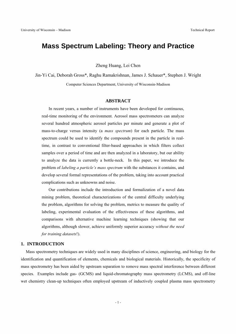
Table 5: Binary Search Procedure We now describe the DB algorithm itself. The algorithm is initialized with a valid label x . It searches outward

from x along each dimension in turn, identifying valid labels in each direction and adding them to a set Q̂ for

further investigation.

Input: : Spectrum b , threshold vector [ ]1 2 1, ,..., ,dt t t t +=

error bound E .

Output: ( )label b

DB()

Seek a such that ( , ) , 0.D Aa b E a≤ ≥

if no such a

then STOP with ( )label ;b =∅

else ( )( ){ }ˆ; , ;D Q x a D←∅ ←

while Q̂ ≠ ∅


- 17 -

remove an element ( ),x D from Q̂ ;

if { }1,2,...,D n=

then ( ) ( ) { }label labelb b x← ∪

else

choose any k D∉ ;

( )( , ) BinarySearch , ;l r x k←

for , 1,...,p l l r= +

define y such that , , ;i i ky x i k y p= ≠ =

{ }( ){ }ˆ ˆ ,Q Q y D k← ∪ ∪

end(for) end(if) end(while)

Table 6: Directional Bounding Algorithm

6. DATA GENERATION

There is a fundamental Cdifficulty in evaluating algorithms for labeling mass spectra: Manual labeling of

spectra (to create training sets) is laborious, and must additionally be cross-validated by other kinds of co-located

measurements, such as traditional filter-based or “wet chemistry” techniques. For any given application,

rigorously establishing appropriate “ground truth” datasets can take months of field-work. In this section, we

describe a detailed approach to synthetic data generation that allows us to use domain knowledge to create

signature libraries and input particle spectra that reflect specific application and instrument characteristics. This

has two important benefits:

• It allows us to compare different labeling algorithms, and to quantify their effectiveness with respect to

important parameters such as noise, unknowns, and ambiguity.

• It allows a domain scientist to generate “labeled” datasets that mimic their application, and to rapidly fine-

tune algorithm settings.

Our generator has two parts: generation of the signature library, and generation of input spectra. We begin

with a collection of real ion signatures, and select a set of n linearly independent signatures to serve as “seeds” for

our generator. New signatures are generated using a non-negative weighted average of seed signatures. The set

of all generated signatures is partitioned into two sets: the signature library, and the unknowns.

The generation of new signatures for the signature library is done in “groups” as follows, in order to control

the degree of (non-)uniqueness, or ambiguity. Each group consists of two “base” signatures from the seeds


- 18 -

(chosen such that no seed appears in multiple groups) plus several “pseudo-signatures” obtained using non-

negative weighted averages of these two signatures. The generated signatures in each group are effectively treated

as denoting new ions in the signature library. Of course, they do not correspond to real ions at all; rather, they

represent ambiguity in that it is impossible to distinguish them from the weighted average of base signatures used

to generate them when labeling an input spectrum that contains ions from this group. Intuitively, the larger the

size of a group, the greater is the ambiguity in input spectra that contain ions from the group; observe that

interference can only occur within groups. We create a total of k groups with i+1 pseudo-signatures in group i.

The set of n original signatures plus the (k+3)k/2 pseudo-signatures generated as above constitute our

“universe” of all signatures. Next, we select some of these signatures to be unknowns, as follows: We randomly

select one signature from each of the k groups; these k signatures are “interfering unknowns”. We also randomly

select u-k seed signatures that were not used in group generation; these u-k signatures are “non-interfering

unknowns”, giving us a total of u unknowns.

The second part of our generator is the generation of input spectra. An input spectrum is generated by selecting

m signatures from the universe of signatures and adding them according to a weighting vector w . Ambiguity and

unknowns are controlled by the careful selection of signatures that contribute to the spectrum, and the input

weighting vector controls the composition of the spectrum as well as the contribution of unknowns. We observe

that the effect of many unknowns contributing to an input spectrum can be simulated by aggregating them into a

single unknown signature with an appropriate weighting vector; accordingly, we use at most a single unknown

signature. Table 11 summarizes the parameters for spectrum generation.

m Number of signatures that contribute to the spectrum.

q Degree of ambiguity, specified in terms of group number.

w

Weighting vector of m elements sorted in descending order,

except the right-most element, which controls the weight of

unknown signature.

o o = 1: unknown signatures is used in spectrum generation;

o = 0: unknown signatures are not used

v v = 1 if unknown signature selected interferes with known

signatures selected. Otherwise v = 0.

g Average amount of noise added to each m/z position.

Table 11: Parameters Used for Spectrum Generation

We begin by randomly selecting two signatures from group q. Then, if unknowns are desired in the generated

spectrum (o=1), we choose either the qth unknown signature, or a randomly selected non-interfering unknown


- 19 -

signature, depending on whether or not the unknown is desired to interfere with known ions in the spectrum (v =

1 or 0). The contribution of unknowns is controlled by the last component of the weighting vector. Next, we

randomly select signatures from the signature library that do not belong to any of the k “groups” to get a total of m

signatures. These signatures are linearly independent seeds, and thus the ambiguity of the generated spectrum

will depend solely on the first 2 (or 3, if an interfering unknown is chosen) signatures.

Finally, we select values for m random variables following a normal distribution whose means are given by the

weighting vector of arity m. The values for these variables are used as the weights wi to combine the m

signatures:∑ −mj jj Sw1 . (We note that when an unknown signature is used in the generation, the last element of the

weighting vector is reset to be the relative quantity of the unknown signature and the whole weighting vector is

normalized to sum up to 1.)

We account for noise by simply adding a noise value (a random variable following a normal distribution) to

each component (i.e., m/z position) of the generated spectrum.

7. EXPERIMENTAL RESULTS

We now describe experiments to evaluate our labeling algorithms with respect to both quality and labeling

speed. To give the reader an idea of the speed, we observed an average processing rate of about 1 spectrum per

second when we ran our algorithms on over 10,000 real mass spectra collected using an ATOFMS instrument in

Colorado and Minnesota; this is adequate for some settings, but not all, and further work is required. Speed and

scalability are not the focus of this paper, but are addressed in [7], and extensive experiments are reported. We

also tested the accuracy of our labeling algorithm against a small set of manually labeled spectra; all were

correctly labeled by the algorithm. Admittedly, this is not an extensive test, but we are limited by the fact that

manual labeling is a tedious and costly process. (This underscores the importance of not requiring training

datasets.)

In this section, we therefore evaluate our algorithms using the data generator from Section 6; this approach

also allows us to study the effect of ambiguity, unknown signatures and noise levels in a controlled fashion. For

comparison, we also evaluated machine learning (ML) algorithms based on WEKA [17]. However, the reader

should note that our algorithms can label input spectra given only the signature library, whereas the ML

approaches require extensive training datasets, which is unrealistic with manual labeling. In addition, the ML

algorithm ignores equivalent alternatives and only generates one label. Nonetheless, we propose two different

quality measures and include the comparison for completeness, and to motivate a promising direction for future

work, namely the development of hybrid algorithms that combine the strengths of these approaches.


- 20 -

7.1 Machine Learning Approach

Our ML algorithm builds upon WEKA classifiers [17]. For each signature in the signature library, we train a

classifier to take a given input spectrum and output a presence category (absent, uncertain or present), i.e., to

detect whether or not the ion represented by the signature is present in the particle represented by the spectrum.

The predictive attributes are the (fixed set of) m/z locations, taking on as values the signal intensities at these

locations in the input spectrum. To label a spectrum, we simply classify it using the classifiers for all signatures in

the library. When we are only interested in the presence of a subset of ions, of course, we need only train and run

the classifiers for the corresponding signatures. We evaluated four types of classifiers: Decision Trees (J48),

Naïve Bayes, Decision Stumps, and Neural Networks. Decision Trees consistently and clearly outperformed the

other three, and we therefore only compare our algorithms against this approach in the rest of this section.

7.2 Datasets

The (common) dimension of all signatures and spectra is set to be 255, which is the value in our real dataset.

We used n=78 base signatures of real ions, and generated k=5 groups containing 2,3,4,5, and 6 pseudo-signatures,

respectively. Including the original 78, we thus obtained 98 signatures, 15 of which were withheld as unknown;

the remaining 83 comprised the signature library. For generating input spectra, we set the number of signatures

used for spectrum generation to be m=10. The relative proportion of these m signatures was controlled by the

weighting vector [0.225, 0.2, 0.2, 0.1, 0.1, 0.06, 0.06, 0.03, 0.01, 0.01]. The weighting vector simulates the fact

that there are usually around 3 majority ions in a particle and 4 to 5 ions of medium quantity.

We generated five testing datasets with controlled ambiguity, unknown signature and noise levels. Each

dataset contains several files, each of which contains 1,000 spectra generated by using the same set of parameter

values. Dataset 1 is designed to test the effect of noise. It consists of 10 files. Each file corresponds to a distinct

noise level from 0% to 360% of a preset error bound3. No ambiguity or unknown signature is involved in this

dataset. Dataset 2 tests the effect of ambiguity. It consists of 5 files corresponding to 5 ambiguity levels. No

unknown signature or noise is introduced in this dataset. Dataset 3 has no noise or ambiguity, but contains some

non-interfering unknown signatures. This dataset contains ten files, with the weight on the unknown signature

varying from 0% to 180% of the preset error bound. Dataset 4 is identical to Dataset 3 except that the unknown

signatures selected are interfering unknowns. Dataset 5 is designed to test the combined effect of noise and

ambiguity. Five ambiguity degrees used in Dataset 2 and five noise levels selected from the 10 noise levels used

in Dataset 1 result in 25 different combinations of noise and ambiguity, and 25 files are generated for each such

combination. The discretization criteria used for all the dataset above is controlled by a threshold vector [0, 0.08,

0.18, 1] which divides the quantity of ion into three categories: absent, uncertain and present.

3 The error bound is set to be 0.01. The noise level represents the overall average amount of noise added to 255 m/z positions. For instance,

at noise level 0.01 (100% of error bound) the expected absolute noise at each m/z position is 0.01/255.


- 21 -

Spectrum

Ion signature A

Ion signature B

Ion signature C

Ion signature D

Figure 5: Indistinguishable Spectrum Labels

7.3 Labeling Quality

Given a particle, consider the “ideal” version of its spectrum obtained by eliminating noise and unknowns, and

is therefore strictly the weighted sum of known ion signatures present in the particle. Even such an ideal mass

spectrum might not have unique labels. The spectrum shown in Figure 5 might represent a particle that contains

ions A and B, or a particle that contains C and D. Given only the input spectrum, the combinations AB and CD

are mathematically indistinguishable, and should be presented to domain experts for further study. The complete

set of such “indistinguishable spectrum labels” for the “ideal” version of an input spectrum is the best result we

can expect from labeling; we call each label in this set a correct label. Intuitively, it is the set of all feasible

combinations of ions in the particle. This is exactly the label set of the ideal spectrum defined in Section 4 (with

the error bound set to 0). By Theorem 7, our algorithms generate this label set when no unknown or noise is

present, i.e., the ideal version is the given input spectrum itself. However, as noise and unknowns are added, the

labels found by our algorithm will no longer the same as the desired set of all correct labels.

Our first proposed metric compares the result of a labeling algorithm with the set of all correct labels. This

metric consists of two ratios: the hit ratio and false ratio. The hit ratio is the percentage of correct labels in the

result set of the labeling algorithm. The false ratio is the proportion of labels in the result set that are not correct

labels. Formally, let the label set of a particle’s ideal spectrum be TL and let the set of labels found by a labeling

algorithm for the particle’s real spectrum under the presence of noise and unknowns be OL :

||/|| TOT LLLRatioHit ∩= ||/|| OTO LLLRatioFalse −=

Experiments under this metric will be called full labeling tests, and are presented in Section 7.3.1.

Our second metric relaxes the requirement of finding the correct combinations of ions, and focuses on the

proportion of individual ions whose presence or absence is correctly classified. Given a collection of interesting

ions, we aggregate the set of correct spectrum labels to obtain a set of ion labels TIL as follows: An ion of interest

is marked present if all correct labels mark it as present, absent if all correct labels mark it as absent, and marked

uncertain in all other cases. Similarly, we can obtain a set of ion labels OIL from the result set of the labeling

algorithm. Our second metric consists of two ratios based on these ion labels:

||/|| TOT ILILILRatioHitPartial ∩= ||/|| OTO ILILILRatioFalsePartial −=


- 22 -

Partial hit ratio is similar to hit ratio, and describes the percentage of ions that are correctly labeled, while partial

false ratio is the proportion of ions that are incorrectly labeled. Experiments under this second metric will be

called partial labeling tests, and are presented in Section 7.3.2.

It is worth noting that for any given spectrum, our algorithms will generate exactly the same result, namely, the

label set of that spectrum. Therefore, for quality evaluation, we simply refer to them as “our algorithm” or the

“LP” algorithm, since they both build upon linear programming.

7.3.1 Full Labeling Tests

In the following graphs, each data point for our algorithm is the average of results on 1000 spectra, while each

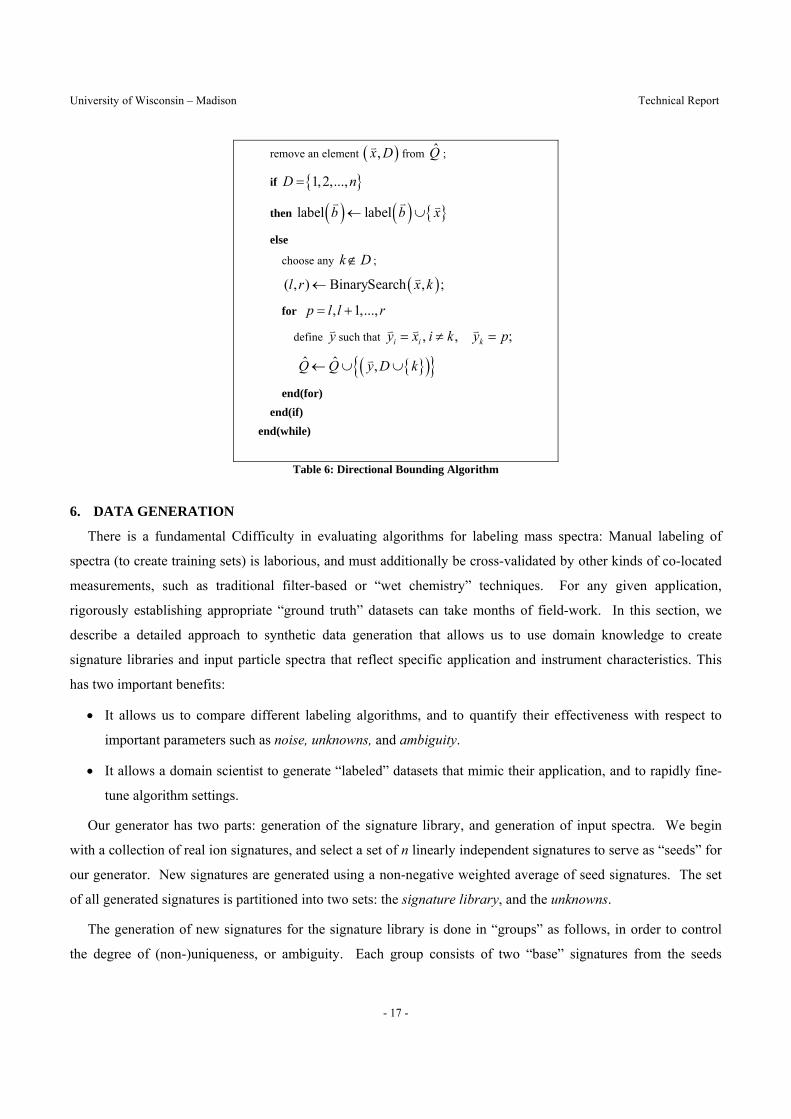
data point for the ML algorithm is the result of 5-fold cross validation on the same 1000 spectra. Figure 6 shows

the result on Dataset 1, which contains no ambiguity or unknowns. In this case, the labeling algorithm is not

required to resolve any ambiguity. Even in this simple case, the ML algorithm performs poorly. Its hit ratio is

close to zero while the false ratio is close to one. In contrast, our algorithm shows great strength in identifying a

possible combination of ions to explain the spectrum. The hit ratio remains almost perfect when the noise is

within 180% of error bound, but drops sharply when noise grows above that threshold. This shows a limitation of

our algorithm: the error bound is the only component that accounts for noise, and our results are sensitive to the

choice of the error bound relative to noise levels. While the error bound helps in accounting for noise, it also

introduces a degree of freedom that allows incorrect labels to be included. Surprisingly, the false ratio, which

measures the percentage of incorrect labels in the result, actually goes down as the noise level increases; the noise

intuitively takes up the slack introduced by error bound. This observation suggests that we might be able to

automatically tune the error bound by estimating the noise level. Figure 7 shows the results on Dataset 5, which

contains both ambiguity and noise. As we can see, the already low hit ratio of the ML algorithm drops further,

essentially to zero, and the false ratio goes over 95%. Our algorithm performs consistently well in Figure 7,

demonstrating its ability to handle ambiguity even in the presence of noise. Figures 8 and 9 summarize the

experimental results on Datasets 3 and 4, which show the effect of unknowns. Intuitively, if the unknown ion is

non-interfering, it acts like additional noise at some m/z positions, which makes it harder to be compensate for.

The hit ratio of our algorithm drops sharply when the non-interfering unknown proportion exceeds the error

bound. The spike in the false ratio at the very end is an artifact caused by the fact that the number of labels found

is reduced to one essentially, and that one is incorrect. The effect of interfering unknowns is more interesting.

While it raises the false ratio as more and more unknowns are added, as expected, surprisingly, it also helps the

hit ratio (because it can be interpreted as some linear combination of known signatures that effectively increases

the quantity of the knowns).


- 23 -

Figure 6: Effect of Noise without

Ambiguity

Figure 7: Effect of Noise with

Ambiguity

Figure 8: Effect of Non-interfering

Unknown

Figure 9: Effect of Interfering Unknown

7.3.2 Partial Labeling Tests

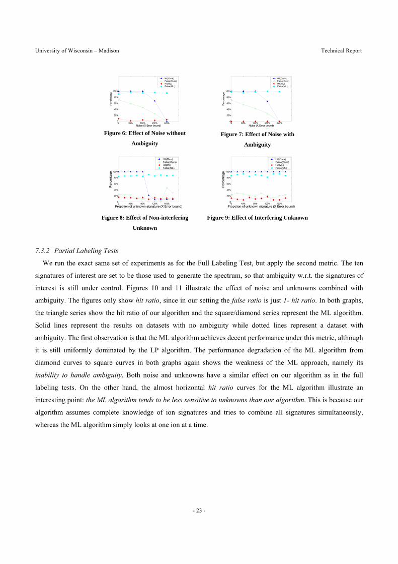
We run the exact same set of experiments as for the Full Labeling Test, but apply the second metric. The ten

signatures of interest are set to be those used to generate the spectrum, so that ambiguity w.r.t. the signatures of

interest is still under control. Figures 10 and 11 illustrate the effect of noise and unknowns combined with

ambiguity. The figures only show hit ratio, since in our setting the false ratio is just 1- hit ratio. In both graphs,

the triangle series show the hit ratio of our algorithm and the square/diamond series represent the ML algorithm.

Solid lines represent the results on datasets with no ambiguity while dotted lines represent a dataset with

ambiguity. The first observation is that the ML algorithm achieves decent performance under this metric, although

it is still uniformly dominated by the LP algorithm. The performance degradation of the ML algorithm from

diamond curves to square curves in both graphs again shows the weakness of the ML approach, namely its

inability to handle ambiguity. Both noise and unknowns have a similar effect on our algorithm as in the full

labeling tests. On the other hand, the almost horizontal hit ratio curves for the ML algorithm illustrate an

interesting point: the ML algorithm tends to be less sensitive to unknowns than our algorithm. This is because our

algorithm assumes complete knowledge of ion signatures and tries to combine all signatures simultaneously,

whereas the ML algorithm simply looks at one ion at a time.


- 24 -

Figure 10: Effect of Noise Figure 11: Effect of

Unknowns

Overall, our algorithm clearly beats the ML algorithm in terms of labeling quality, even in partial labeling tests.

In addition, the ML algorithm needs substantial training data. This is not realistic to get at all. However, the ML

algorithm does show promise in partial labeling, which suggests a promising research direction, namely a hybrid

algorithm that combines the speed of ML and the ambiguity-handling ability of our LP-based approach.

Figure 12: Effect of Ambiguity on Label

Time

Figure 13: Scalability with Respect to #

Signatures

7.4 Labeling Speed

We ran efficiency tests on the five datasets described in Section 7.2. Results show that the presence of noise

and unknown signature does not affect the performance of our algorithms much, unless the noise or weight on the

non-interfering unknown signature is significantly larger than the error bound. When no ambiguity is present,

labeling takes about one second for both DFS and Crawling algorithms. However, as more ambiguity is included

and the label set size increases sharply, the performance of our algorithms degrades significantly. Figure 12 shows

the running time of our algorithms on Dataset 2, which contains five files of spectra with five different degrees of

ambiguity. Series 1 and 2 show the performance of DFS and Crawling algorithms. The Crawling algorithm

exploits the convexity of the distance function and runs slightly faster than DFS, but both become much slower as

ambiguity is increased. This is mainly due to the dramatic increase in the number of correct labels. The ML

algorithm is much faster than our algorithms, but it is worth noting that when no ambiguity is involved and the

number of correct labels is small, the running time of our algorithm is almost the same as for ML. In addition, the

training time of the ML approach is not reflected at all in these graphs. Further, when we are only interested in

detecting a small number of signatures, we can revise our DFS algorithm to only pick the signatures of interest

and do partial labeling. This optimization greatly speeds up DFS, to about 100 spectra per second. Figure 10

summarizes the results of algorithm scalability with respect to the number of signatures in the signature library.


- 25 -

We have not discussed efficiency issues in any depth, since this is not the focus of this paper. While some major

performance results are included here for completeness, we address running time improvement and scalability

issues in a separate paper [7].

8. CONCLUSION

Methods of categorizing aerosol particles using clustering and neural networks have been proposed [1,11,9,15],

but none of them deals with the labeling problem directly. The linear programming method used in this paper is

standard, see, e.g., [12]. Related nonlinear or integer programming tasks arising from the use of Euclidean

distance or discretization are also well studied in the optimization community [6,12,18]. Recent work on

knowledge-based optimization and machine learning [8,16] are promising extensions to the framework we

propose. Machine learning methods such as clustering [5,19] can be applied to our basic linear programming

approach by helping identify better initial points and optimization constraints.

Finally, while this paper addresses foundations and evaluates quality of labeling, in a related paper [7], we

have studied how to scale our labeling algorithms to label a large group of spectra. There are several directions for

future work:

• Better labeling algorithms: Can we use the algorithms presented here to label spectra, and use the results as

training sets for machine learning algorithms? Can we adaptively “learn” important parameters such as the

error bound? The overall objective is a fast hybrid algorithm that does not require manually labeled training

data and that can adapt to changing input streams automatically.

• Utilizing domain knowledge for labeling: Scientists usually have a priori knowledge about spectra they

collect, e.g., if ion A appears in one particle, then it is likely that ion B will also appear in the same particle.

How can we let them specify this information and exploit it for better labeling? As another example,

domain knowledge could be used to produce synthetic training data that closely mimics expected real-

datasets, using the detailed generator that we described.

• Discovering unknown signatures: A limitation of our framework is that it does not distinguish between

noise and unknown signatures, and the precision of labeling is influenced by the existence of unknowns.

Can we discover unknowns?

• Applying our techniques to diverse real datasets: In this paper, we have abstracted many complications that

arise in practice. This work is part of the EDAM project, an ongoing collaboration between chemists and

computer scientists, and we plan to validate our techniques by applying them to real spectral datasets, with

“ground truth” data collected simultaneously using filter-based techniques. This will also allow us to

explore accurate calibration of quantity information.


- 26 -

9. REFERENCES [1] Agrawal, R., Imielinski, T., Swami, A., Mining Associations between Sets of Items in Massive Databases, Proc. ACM-SIGMOD,

1993.

[2] Agrawal, R., Faloutsos, C. and Swami, A. Efficient Similarity Search in Sequence Databases. Proc. Conf. on Foundations of Data

Organization and Algorithms, 1993.

[3] Agrawal, R., Mannila, H., Srikant, R., Toivonen, H. and Verkamo, A. I., Fast Discovery of Association Rules, Advances in

Knowledge Discovery and Data Mining, 1995.

[4] Agrawal, R. and Srikant R.: Fast Algorithms for Mining Association Rules, Proc. VLDB, 1994

[5] Basu, Sugato, Banerjee, Arindam and Mooney, Raymond J., Semi-supervised Clustering by Seeding. Proc. ICML, 2002.

[6] Benson, Steven J., More, Jorge J, A Limited Memory Variable Metric Method, in Subspaces and Bound Constrained Optimization

Problems, 2001.

[7] Chen, L., Huang, Z. and Ramakrishnan, R., Cost-Based Labeling of Groups of Spectra, Proc. ACM-SIGMOD, 2004.

[8] Fung, G., Mangasarian, O.L. and Shavlik, J., Knowledge-Based Support Vector Machine Classifiers. Proc. NIPS 2002.

[9] Gard, E., Mayer J.E., Morrical, B.D., Dienes, T., Fergenson, D.P. and Prather, K.A., Real-Time Analysis of Individual

Atmospheric Aerosol Particles: Design and Performance of a Portable ATOFMS, Anal. Chem. 1997, 69, 4083-4091.

[10] McCarthy, J., Phenomenal data mining, In Communications of the ACM 43(8), 2003

[11] Noble, C.A. and Prather K.A., Real-time Measurement of Correlated Size and Composition Profiles of Individual Atmospheric

Aerosol Particles. Environ. Sci. Technol, 1996; 30, 2667-2680.

[12] Nocedal, J. and Wright, S.J., Numerical Optimization, Springer, 1st edition, 1999.

[13] Prather, K.A., Nordmeyer, T., and Salt, K. Real-time Characterization of Individual Aerosol Particles Using ATOFMS. Anal.

Chem., 1994; 66, 1403-1407.

[14] Srikant, R. and Agrawal, R., Mining Quantitative Association Rules in Large Relational Tables, Proc ACM-SIGMOD, 1996.

[15] Suess, D.T. and Prather K.A., Mass Spectrometry of Aerosols, Chemical Reviews, 1999, 99, 3007-3035.

[16] Towell, G.G. and Shavlik J., Knowledge-Based Artificial Neural Networks. Artificial Intelligence, 70, 1994.

[17] Witten, Ian H. and Frank, Eibe, Practical Machine Learning Tools and Techniques with Java Implementation, Morgan Kaufmann,

1999.

[18] Wolsey, L., Integer Programming, John Wiley, 1998.

[19] Zhang, T., Ramakrishnan, R. and Livny M., BIRCH: An Efficient Data Clustering Method for Very Large Databases, Proc. ACM-

SIGMOD, 1996.

Appendix A

THEOREM Consider signature library ] ,...,,[ 21 nsssA = and a spectrum b where nsss ,...,, 21 are linearly independent (i.e., there is

no vector a = 1 2[ , ,..., ]na a a such that ∑ =ni ii sa1 and at least one 0ia ≠ ). Then, either b has the unique labeling property w.r.t. A, or the

system of equations

Ax b= , 0x ≥ (1)

has no solution.


- 27 -

PROOF If b cannot be uniquely labeled and equation (1) has a solution, there must exist two vectors 0x and 1x such that

0Ax b= , 0 0x ≥ (2)

1Ax b= , 1 0x ≥ (3)

1 0x x≠ (4)

Subtract (3) from (2), we have 0 1( ) 0A x x− = . Since 1 0x x≠ , vector 0 1( ) 0x x− ≠ . It violates the precondition that nsss ,...,, 21

are linearly independent. Thereby, b must have the unique labeling property or equation (1) does not have a solution.

Appendix B

THEOREM: Consider signature library ] ,...,,[ 21 nsssA = and a spectrum b where nsss ,...,, 21 are not linearly independent. If there is a

solution ],...,,[ 21 naaaa = to Ax b= , 0x ≥ such that 0,...,2,1 >= ini amin , then b has infinitely many labels.

PROOF Since nsss ,...,, 21 are not linearly independent, by the definition, there exists a vector a = 1[ ,..., ]ma a , such that

0Aa = . Let constant h be( )

(| |)i

i

Min xMax a

. Then for any constant f, 0<f<h, the vector 0fa x+ ≥ . In addition,

( ) 0A fa x fAa Ax b b+ = + = + = . So, for any f, 0<f<h, fa x+ also satisfies equation Ax b= , 0x ≥ and thus is a possible labeling for the input spectrum too. Given a h>0, the number of f’s is infinite, thereby the number of possible labels for spectrum

b is also infinite.

Appendix C

A linear programming algorithm to test the unique labeling property of spectrum b

Input: Signature database matrix A. A : n m×

Spectrum b . b is a vector of length n

Output:

True, if b has the unique labeling property with respect to A

False, if b does not have the unique labeling property with respect to A

Procedure:

Seek a s.t. A a = b , 0a ≥ (1)

*a is the feasible solution obtained in (1)

Define *{ | [ ] 0}J j a j= >

*{ | [ ] 0}CJ j a j= =

For k = 1 to n


- 28 -

Seek d s.t. A d =0 (2)

[ ] 0 Cd j if j J≥ ∈

[ ] 1d k =

If (2) succeeds Return False

For each k J∈

Seek d s.t. A d =0 (3)

[ ] 0 Cd j if j J≥ ∈

[ ] 1d k = −

If (3) succeeds Return False Return True End of Procedure Note: (1), (2), (3) will call a standard linear programming procedure. Proof:

Necessary condition

Suppose the algorithm returns True, but b does not have the unique labeling

property with respect to A. There must exist a e s.t.

A e = b , 0e ≥

*e a≠

Define *h e a= −

*{ | [ ] 0}J j a j= >

*{ | [ ] 0}CJ j a j= =

Since 0e ≥ , [ ] 0 Ch j if j J≥ ∈

Since *e a≠ , there must be a k s.t. [ ] 0h k ≠ .

If [ ] 0h k > , 1[ ]

hh k

is a feasible solution for (2)

The program will return False.

Otherwise, [ ] 0h k < , 1[ ]

hh k

is a feasible solution for (3)

The program will return False too.


- 29 -

Therefore, b must have the unique labeling property.

Sufficient condition Suppose the algorithm returns False, the linear programming in (2) or (3) must succeed.

If (2) succeeds, the feasible solution is 1d .

Let *

1

(| [ ] |)(| [ ] |)

Min a iMax d i

α =

Both α 1d + *a and *a are solutions to the equation Ax b= , 0x ≥ and α *1d a≠ .

Otherwise, (3) succeeds, the feasible solution is 2d .

Let *

2

(| [ ] |)(| [ ] |)

Min a iMax d i

α =

Both α 2d + *a and *a are solutions to the equation Ax b= , 0x ≥ and α *2d a≠ .

Therefore, b does not have the unique labeling property.

Appendix D

Given a set of points rS ⊆ ℜ , the affine subspace generated by S is defined as

1 1( ) { | 1, 1, , ,1 }

m m

i i i i ii i

as S w s m w w R s S i m= =

= ≥ = ∈ ∈ ≤ ≤∑ ∑

The convex hull generated by S is defined as

1 1( ) { | 1, 1, 0, ,1 }

m m

i i i i ii i

ch S w s m w w s S i m= =

= ≥ = ≥ ∈ ≤ ≤∑ ∑

Such an expression 1

ni ii

w s=∑ with the constraints as in the definition of ( )ch S is called a convex combination.

Clearly ( ) ( )ch S as S⊂ , but has the same dimension.

We will assume our set 0 1{ , ,..., }nS s s s= is finite, and all is lie on the hyperplane T: 1sη =∏ , ,where (1,...,1)T rη = ∈ℜ . Then ( )as S , in particular, ( )ch S , all lie on this hyperplane ∏ . Hence d = dim(as(S)) ≤ r − 1. We

denote by A the r × (n + 1) matrix [s0, s1, . . . , sn].

Define a set {s0, . . . , sk} to be affine independent, if whenever 1

0ki ii

w s=

=∑ , with 1

0kii

w=

=∑ then all wi = 0.


- 30 -

CLAIM 1 {s0, s1, . . . , s1} is affine independent iff {s1 − s0, . . . , sk − s0} is linearly independent.

CLAIM 2 If {s0, s1, . . . , sk} ⊂ Π, then it is linearly independent iff it is affine independent.

We show affine independence implies linear independence for S ⊂ Π. Suppose 1

0ki ii

w s=

=∑ , then

1 0( ) 0k kT

i i ii iw w sη

= == =∑ ∑ , and thus all wi = 0.

( )ch S is a convex polytope of dimension d. As such it is endowed with the Euclidean metric

and topology of as(S). We denote by X0 the interior points of X.

LEMMA 1 If x ∈ ch(S)o then x has a convex combination 1

ki ii

w s=∑ where all wi > 0.

Consider any si. We first obtain a convex combination for x in which the coefficient of si is positive. If x = si then this is trivial. Suppose ix s≠ . Let the 1-dimensional ray from si to x intersect the boundary of ch(S) at y. Then clearly x lies strictly between si and y. So, ix = s + (1- )y,α α where α > 0. Now substitute y by its convex combination from S, we get a convex combination of x where the coefficient of si is positive. To complete the proof of the lemma we simply take an average of such expressions, one for each si.

LEMMA 2 If 1

ki ii

x w s=

= ∑ , where { si | wi > 0 } has rank d + 1, then ( )ox ch S∈ . Wolog, {si, s1 . . . , sd} has rank d + 1, with w0,w1, . . . ,wd > 0. Then affine independent and {s0, s1 . . . , sd} spans a simplex ∆. Let

0

dii

wα=

= ∑ . If α = 1

(i.e., there are no other positive coefficients in 1

ki ii

x w s=

= ∑ ) then clearly ( )o ox ch S∈∆ ⊆ . If α < 1, then x can be expressed as a convex sum

' (1 ) ''x x xα α= + −

where 0

' ( / )d oi ii

x w sα=

= ∈∆∑ , and 1

'' ( /(1 )) ( )ni ii d

x w s ch Sα= +

= − ∈∑ . By varying 'x within the open set o∆ , we see clearly that ( )ox ch S∈

Corollary 1 A point ( )x ch S∈ is an interior point iff it has a convex combination where all coefficients are positive. It is perhaps tempting to think that every interior point x always has a “pure” convex combination where exactly d +1 coefficients are positive corresponding to some d+1 affine independent si. This is not true. An example is the d-dimensional octahedron, the convex hull spanned by the 2d unit vectors ±ei, 1 ≤ i ≤ d. Consider the point 0. Clearly, by taking inner product with ei, any convex combination of 0 must be of the form ( ( ))i i i ii

w e w e+ −∑ . Thus if 0 were to be in the interior of any simplex of dimension > 1, then at least two pair, ±ei and ±ej, have wi,wj > 0. But these 4 vectors are already affine dependent. Another caution we observe from this example is that even though there are only 2d vertices, the octahedron as its convex hull has 2d facets. Thus it is in general infeasible to enumerate all the facets of ( )ch S computationally.

LEMMA 3 If S is affine independent, then every point in ch(S) has a unique convex combination. If S is affine dependent, then every interior point of ch(S) has infinitely many convex combinations.


- 31 -

PROOF The first claim is obvious: If S is affine independent, and 1 1

'i i i ii ix w s w s

= == =∑ ∑ , then ( ' ) 0i i ii

w w s− =∑ , with ( ' ) 0i ii

w w− =∑ . Therefore by affine independence, all 'i iw w= Now suppose S is affine dependent. There exists some 0i ii

w s =∑ , with 0iiw =∑ , for wi not all zero. We may assume all | |iw ε< for sufficiently small ε > 0.

Now add this sum to a convex combination of x with all positive coefficients. The result follows. So assuming S is affine dependent, which necessarily is the case for n ≥ r, the only possible case for unique convex combination is on the boundary of ( )ch S .

Consider the following algorithm: Given any b. Solve for the feasibility of the linear programming: Find w = (w0,w1, . . . ,wn)T, such that

0, 1, 0n

i iiAw b w w

== = ≥∑ . This is solvable for w iff ( )b ch S∈ . Suppose

0

ni ii

b w s=

= ∑ is one such solution. Let B = { si | wi > 0 }. If B is affine dependent, then return “non-unique”. Suppose B is affine independent. Let P be the affine subspace generated by B. Let π be a linear projection dℜ along P, so that P is projected to a single point, and dim(π( dℜ )) = d − dim(P). We may assume π(P) = 0, since we are dealing with convex combinations in affine geometry. Let C = ch(S − B), and C = ch(π(S − B)). Clearly C = π(C). Now by solving a linear programming problem we can determine if 0 (= π(b)) is in C. If so, return “non-unique”, otherwise return “unique”. THEOREM 1 For any ( )b ch S∈ , the above algorithm solves the problem of whether b has a unique convex combination in S. PROOF Suppose ( )b ch S∈ . If B is affine dependent, then on P, b is an interior point of ch(B) by Corollary 1, and therefore by Lemma 3, b has non-unique convex combinations. Now we assume B is affine independent, dim(P) = |B| − 1, and b is an interior point of the simplex ( )ch B .

We have a convex combination of b over :i

i is BB b w s

∈= ∑ . If b does not have a unique convex combination from

S, then there is another expression 'i iib w s=∑ . Since B is affine independent, the non-zero coefficients among 'iw

can not be all from { | }ii s B∈ . Let some ' 0iw > for js B∉ . Under the projection π, all terms corresponding to is B∈ disappeared, we get 0 ( ) ' ( )b w sπ π= =∑ , where the second sum involves only terms not in B, but does contain

' ( )j jw sπ with non-zero ' jw . By dividing out the sum of these coefficients ' 0w >∑ , we get a convex combination of 0 = π(b), i.e., 0 ∈ C. Conversely assume 0 = π(b) ∈ C. Let 0 ' ( )w sπ=∑ be a convex combination, where all terms s B∉ . Now we can lift this back to dℜ to get some convex combination for a certain point x P∈ , i ix w s=∑

where the sum is over all terms s B∉ . Now if x = b then we are done, having obtained a different convex combination for b than i ii

b w s=∑ among is B∈ . (In fact a weighted sum gives infinitely many different convex combinations.) Suppose x b≠ . Draw a ray from x toward b, which intersects at y with the boundary of the simplex generated by B. This y has a convex combination among vectors from B, and b can be expressed as a weighted sum of x and y. Using the convex combination of x above with s B≠ , we obtain another convex combination for b where not all positive coefficients are among B. This is different than i ii

b w s=∑ among si ∈ B (and hence, by any weighted average we get infinitely many different convex combinations.) The theorem is proved.


- 32 -

We note that if the points on the boundary of ch(S) are all on general position (i.e., no two coincide, no three colinear, . . ., in general any k + 1 points have affine rank k) then every point on the boundary has unique convex combination.

Appendix E

LEMMA 1 Suppose we have a convex set K contained in the unit cube [0,1]nQ = . If Q is divided

along every dimension into half, obtaining 2n (closed) subcubes. Suppose K intersects at most n of these subcubes. Then there exists a dimension i, 1 ≤ i ≤ n, where K is either contained in the first half: 0 ≤ xi ≤ 1/2, or contained in the second half: 1/2 ≤ xi ≤ 1. This statement can be generalized. A straightforward induction proves the following. THEOREM Suppose we have a convex set K contained in some “brick” B = [L1, U1] × [L2, U2] ×· · · × [Ln, Un]. Assume B is divided into ir ranges along each dimension i, Li = ai,0 < ai,1 < ai,2 < · · · < ai,ri = Ui, and B is the union of

1

nii

r=∏ many “subbricks” of the form [a1,j1, a1,j1+1]× [a2,j2, a2,j2+1] × · · · × [an,jn, an,jn+1]. Suppose K has

only non-empty intersection with at most n of these subbricks, then there exists a dimension i, 1 ≤ i ≤ n, and a “slice” { x ∈ B | xi ∈ [ai,ji, ai,ji+1] } which contains K. Thus, in our context, if the convex set of solutions K does not intersect many subranges, then the problem can be effectively reduced in dimension, until the number of relevant subranges which do intersect K. Now we turn to the proof of the Lemma. First we observe that it is crucial that we speak of “closed” subcubes. If we were to consider “open” subcubes, then there is the counter example of the diagonal straight line segment as our set K. Also the number n is optimal, as demonstrated by the example of a simplex with vertices at 0 and at vi, 1 ≤ i ≤ n, where vi has coordinates 3/4 in dimension i and 0 elsewhere. PROOF We prove the Lemma by induction on n. The base case n = 1 is trivial. For any binary string {0,1}nb∈ , we denote by n

bQ the subcube where 0 ≤ xi ≤ 1/2 if bi = 0 and 1/2 ≤ xi ≤ 1 if bi = 1. By assumption { | }n

bb K Q∩ ≠ ∅ has cardinality at most n.

Consider the orthogonal projection 1: n nπ −ℜ →ℜ , where 1 1 1 1( ,..., , ) ( ,..., )n n nx x x x xπ − −= . Let ' ( )K Kπ= . Among the 2 1n − subcubes of [0, 1]n−1 of the form 1

'nbQ − , where 1' {0,1}nb −∈ , if 'K only intersects at most n−1 of them, then by

induction, there exists a dimension 1 ≤ i ≤ n−1, such that 'K is contained in either the first half or the second half along that dimension. Then clearly, in nℜ , K is also contained in either the first or the second half along that dimension.

Therefore we may assume that there are n distinct subcubes ' ' '1 2

1 1 1, ,...,n

n n nb b b

Q Q Q− − − , with which 'K has a non-empty intersection. Let '

1' 'j

nj b

p K Q −∈ ∩ , for 1 ≤ j ≤ n. (Note that ' jp ’s need not be distinct.) Let pj ∈ K such that ' ( )j jp pπ= .

We write ( ' , )j j jp p t= , where 1' {0,1}njp −∈ and 0 ≤ tj ≤ 1.

If tj ≤ 1/2, then K has a non-empty intersection with the subcubej

nb

Q , where ' 0j jb b= .Similarly if tj ≥ 1/2 then K

has a non-empty intersection with the subcubej

nbQ , where ' 1j jb b= . We have obtained at least n subcubes

j

nbQ , each

has a non-empty intersection with K. Note that these n binary strings b1, . . . , bn are all distinct (because 1' ,..., 'nb b are all distinct, even though the points 1' ,..., 'np p need not be distinct.)


- 33 -

(If some tj = 1/2, then we have actually obtained n+1 subcubes, and the proof is finished. So we may assume none of tj = 1/2 and each bj is unambiguously defined.) Assume K is not contained in the first half or the second half along dimension n, then it can ot be the case that all tj ≤ 1/2 or all tj ≥ 1/2. It follows that there are some 1 ≤ j ≠ k ≤ n, such that tj > 1/2 and tk < 1/2. In particular, j kp p≠ .

Consider the line segment from pj to pk. There exists a unique point p along this line segment where the n-th coordinate is exactly 1/2. By convexity of K, p ∈ K. Write 1 2 1( , ,..., ,1/ 2)np x x x −= .

Define 1' [1... 1] [0,1]nb b n −= − ∈ as follows: For 1 ≤ j ≤ n − 1, if xj ≤ 1/2 then b[j] = 0, and otherwise b[j] = 1. Then let '0b b= and * '1b b= . Clearly n

bK Q∩ ≠ ∅ and *

nb

K Q∩ ≠ ∅ , because both contain p.

We claim at most one of nbQ or *

nb

Q can be among the previous n subcubes j

nbQ , 1 ≤ j ≤ n. This is because both

nbQ and *

nb

Q project under π to the same 1'

nbQ − and yet all n subcubes

j

nbQ project to distinct n − 1 dimensional

subcubes 1' j

nbQ − .

mass spectrum labeling: theory and practiceresearch.cs.wisc.edu/edam/spectrumtr.pdf · mass...

Documents