mass and energy exchange of a plantation forest in scotland
TRANSCRIPT
Mass and Energy Exchange of a Plantation Forest in Scotland Using
Micrometeorological Methods
Robert J. Clement
A thesis submitted for the degree of Doctor of Philosophy
University of Edinburgh
July 2004

Declaration
This thesis has been composed by myself from the results of my own work, except
where stated otherwise, and has not been submitted in any other application for a
degree.
Robert J. Clement
July, 2004
ii

Dedication I dedicate this thesis to my Mother and Father, who have blessed me with an
admiration of nature. Their patience, encouragement and love have sheltered me in
the hardest of times and inspired me with the freedom to err and thrive at all times.
iii

Acknowledgements Much gratitude is due to my advisors John Moncrieff and Paul Jarvis. Their support
and tolerance have allowed the development of this thesis and the idea’s contained
within its pages. I wish also to thank my examiners Ray Leuning and the internal
reviewer for their selfless examination of this extensive manuscript.
Many thanks go to Keith McNaughton who maintained that fine line between interest
and boredom in difficult topics, and whose darkening of my door was equally
matched by mine of his. Kate Heal was most helpful in her assistance in determining
site DBH and provision of throughfall and stream flow data. Matt Williams and
Belinda Medlyn are thanked for provision of model results for comparison with
measured data and Colin Legg for attempting to answer my odd statistics questions.
John Grace, Maurizio Mencuccini, and Keith Smith were most useful for sharing the
occasional beer, meal, and random discussion.
Thanks go to Allan Kelly, John Massheder, and Ford Cropley for listening to my
questions about programming and for giving useful answers which helped to move
EdiRe along to a successful conclusion. Also of invaluable help were the EdiRe users
Allesandro Cescatti, Colin Lloyd, Hank Loescher, Sune Moller, Ed Swiatek, and
Georg Wolfhart who helped find and solve many of the problems encountered during
development.
The efforts of Steve Scott in getting the Griffin site up and running and construction
of the Edibox and the power system were invaluable and the contributions of Lisa
Wingate’s on site field work and analysis helped to fill many gaps in the Griffin
results. I would also like to thank her for keeping me awake on the trips back and
forth to Griffin. Also, Franz Conen was a most helpful and friendly companion and
contributed his soil carbon measurement results. On the more theoretical end of the
task, I would like to thank John Finnigan, Bart Kruijt, Yadvinder Mahli, Patrick Meir,
and Mark Rayment for their help in answering questions about the myriad of
theoretical and analytical details associated with the results from this experiment. I
would also like to thank Jamie Trembath for keeping our field sites running while I
wrote up this experiment and for being a clever fellow.
iv

Others have contributed their time in listening to my complaints and have been good
and understanding friends when the need arose. I would like to thank Allen Young,
Sandra Patino, Mike Clearwater, and Caroline Nichol for helping to share the mental
and emotional load of doing a PhD. There are many others in the department who I
also thank for their cheerful friendliness: Jordi Martinez-Valialta, Emiliano Pegararo,
Ana Ray, Fiona Carswell, Gail Jackson, Sophie Hale, Maree Lucas, and Peter Levy
always had smiles on their faces and a nice word to say, so thank you.
There were many staff at the university who were most helpful throughout the course
of my study. In particular I would like to thank Sheila Wilson, Connie Fox, Graham
Walker, and Derek Scott for their organizational contributions and Bob Astles, Andy
Gray, and Malcolm Ritchie and the numerous servitors for the more practical aspects
of research within the confines of the Darwin building. Also, the fine workmanship
of Alex, Dave, Graeme, George, and Peter from the workshop were crucial in creating
some of the equipment used in the field and in keeping some of the vehicles running.
Last, I would like to thank my many flatmates: Jane Norton, James Hepher, Sara
Marrow, Mark Goodwill, Ingo, Miga, Hazel, Gareth, and that other guy who’s name I
forget. You mostly a pleasure and at worst interesting, but I will always remember
you – even the last guy.
Tillhill Forestry Ltd. made the Griffin research site available for our use and I wish to
thank them for making this research possible.
Research for this project was carried out under EU grant ENV4-CT95-0078, a
bridging grant from the Scottish Forestry Trust, and NERC grant
NER/B/S/2001/00352.
v

Abstract This thesis presents the energy, water, and carbon budgets of a Sitka spruce plantation
forest in Scotland over the period 1997 to 2001. The site’s infrastructure, layout, and
methods employed in site operation are described and a detailed analysis of the
temporal and environmental dependencies of microclimatological measurements is
presented. The site microclimate is observed to be strongly influenced by the site’s
oceanic climate, and canopy development. Atmospheric structure is observed to
affect temporal patterns of microclimatological variables while topography is
observed to affect microclimatological and flux measurements. Eddy covariance flux
measurement theory and methods are examined and specific inadequacies are
addressed. Theoretical aspects of eddy covariance that were examined include signal
despiking, coordinate rotation, low frequency flux contributions, as well as
corrections for density fluctuations, angle of attack errors, and sonic temperature
determination. An analysis of frequency response correction methods was used to
determine if superior methods could be identified. Fluxes of momentum were used to
verify existing measures of atmospheric turbulence and analysed to identify canopy
structure and growth. Sensible heat fluxes were found to have an unexpected
negative bias, only a portion of which can be attributed to instrument error. This bias
is found to depend upon topography and wind speed but is apparently unrelated to
katabatic flow. Large errors in latent heat flux were caused by enhanced tube
attenuation and were corrected using improved frequency response corrections.
Interannual variability of momentum and sensible heat flux were closely associated
with wind speed variability, while interannual variability of net ecosystem exchange
was attributable primarily to radiation. The source of variability of latent heat flux
was not clearly identifiable. Missing values of latent heat flux were modelled using a
canopy conductance model, which incorporated effects of canopy evaporation.
Missing values of nocturnal net ecosystem exchange were obtained using a
temperature dependent model of ecosystem respiration. This model incorporated
effects of friction velocity and topography. Diurnal values of net ecosystem exchange
were modelled using a light response model of gross ecosystem exchange. This
model included dependencies on temperature, vapour pressure deficit, and cloudiness.
A comparison of measured net ecosystem exchange data with the output of two
vi

models suggests that a diurnal version of the nocturnal flux loss problem may exist.
The hydrology budget losses are within (~10%) of precipitation gains and energy
budget components obtained 90% closure. Annual net ecosystem uptake for Griffin is
estimated as 749 g m-2, and residuals of the carbon budget components fall within the
range of experimental measurements.
vii

Table of Contents
Title Page………………………………………………………..………… i
Declaration…………………………………………………………..……. ii
Dedication…………………………………………………..…………….. iii
Acknowledgements………………………………………..……………. iv
Abstract……………………………………………………..…………….. v
Table of Contents…………………………………………..……………. vii
Symbols………………………………………………………..………….. xii
Chapter 1 Introduction…………………………………….…………… 1
Chapter 2 Experiment site……………………………………..……… 11
2.1 Site natural history…………………………………………….. 11 2.2 Site selection…………………………………………………… 13 2.3 Site infrastructure……………………………………………… 13 2.3.1 Access…………………………………………………………….. 14 2.3.2 Power…………………………………………………………….. 14 2.3.3 Towers…………………………………………………………… 20 2.4 Experiment sites……………………………………………….. 21 2.4.1 Sample plots……………………………………………………… 21 2.4.2 Microclimate measurement sites………………………………… 24 2.4.3 Flux measurement site…………………………………………… 24 2.5 Site management……………………………………………… 27 2.5.1 Land use…………………………………………………..……… 27 2.5.2 Site preparation and planting……………………………………. 27 2.5.3 Fertilization……………………………………………………… 29 2.6 Canopy description……………………………………………. 29 2.6.1 DBH, basal area, and biomass…………………………………… 30 2.6.2 Height……………………………………………………………. 35
2.6.3 Canopy dimensions………………………………………………. 37 2.6.4 Litter fall…………………………………………………………. 38 2.6.5 Leaf area…………………………………………………………. 44
2.7 Soil description……………………………………………….. 44 2.7.1 Structure…………………………………………………………. 45 2.7.2 Bulk density……………………………………………………... 46
viii
2.7.3 Nutrient content…………………………………………………. 48 2.8 Summary………………………………………………………. 51
Chapter 3 Canopy microclimate measurement techniques…….. 53
3.1 Sampling of climatological variables…………………………… 53 3.2 Data acquisition………………………………………………… 55 3.3 Instrument deployment…………………………………………. 57 3.4 Data logistics…………………………………………………... 61 3.5 Data quality assessment……………………………………….. 63
3.5.1 Quality assessment concepts………………………………………. 63 3.5.2 Quality control methods…………………………………………… 65 3.5.3 Quality control effects………………………………………..…… 68
3.6 Summary………………………………………………………... 69
Chapter 4 Griffin climatology…..…………………………………….. 71
4.1 Introduction…………………………………………………….. 71 4.2 Global short-wave irradiance…………………………………. 71 4.3 Global PAR……………………………………………………. 78 4.4 Diffuse radiation……………………………………………… 84 4.5 Reflected short-wave radiation and PPFD……………………. 86 4.6 Albedo and Qpg/Qpr ratio……………………………………… 90 4.7 Absorbed and intercepted PAR………………………………. 95 4.8 Net radiation…………………………………………………. 98 4.9 Temperature………………………………………………….. 102
4.9.1 Above canopy air temperature………………………………….. 102 4.9.2 Temperature profiles……………………………………………. 107 4.9.3 Bole temperatures………………………………………………. 111
4.10 Humidity……………………………………………………. 111 4.10.1 Above canopy humidity….……………………………………. 112 4.10.2 Humidity profiles……………………………………………… 115
4.11 Carbon dioxide……………………………………………… 117 4.11.1 Above canopy CO2……………………………………………. 117 4.11.2 CO2 profiles……………………………………………………. 118
4.12 Wind speed…………………………………………………. 119 4.12.1 Above canopy wind speed…………………………………….. 120 4.12.2 Wind speed profiles…………………………………………… 123
4.13 Wind direction……………………………………………… 128 4.14 Precipitation…………………………………………………. 133
4.14.1 Precipitation…………………………………………………… 133 4.14.2 Throughfall, stem flow, and stream flow……………………… 136
4.15 Atmospheric pressure………………………………………. 139 4.16 Soil moisture……………………………………………….. 141 4.17 Soil heat flux………………………………………………. 143 4.18 Summary……………………………………………………. 146
Chapter 5 Ecosystem Exchange Measurement Methods……… 149
5.1 Introduction…………………………………………………… 149 5.2 Theory………………………………………………………… 153
ix

5.2.1 Description of terms…………………………………………… 155 5.2.1.1 Variable of interest……………………………………… 155 5.2.1.2 Assumptions……………………………………………… 155 5.2.1.3 Source term………………………………………………. 155 5.2.1.4 Diffusion terms………………………………………….. 155 5.2.1.5 Storage Term…………………………………………….. 156 5.2.1.6 Transport terms……………………………………….… 158
5.2.2 Implications for measurements…………………………………… 159 5.2.2.1 Implications for flux measurement term……………… 159 5.2.2.2 Implications for storage measurements……………….. 160 5.2.2.3 Implications for experiment design……………………. 161
5.3 Data acquisition and processing……………………………….. 165 5.3.1 Data management………………………………………………… 165 5.3.2 Data processing…………………………………………………… 165
5.3.2.1 Data extraction and conversion………………………… 165 5.3.2.2 Run length………………………………………………… 166 5.3.2.3 Quality assessment………………………………………. 167 5.3.2.4 Noise and despiking…………………………………….. 167 5.3.2.5 Rotation……………………………………………………. 171 5.3.2.6 Intake tube adsorption/desorption ……………………. 178 5.3.2.7 Filtering/detrending……………………………………... 181 5.3.2.8 Low frequency flux information……………………… 182 5.3.2.9 Density effects……………………………………………. 186 5.3.2.10 Frequency response…………………………………….. 189 5.3.2.11 Storage…………………………………………………… 203 5.3.2.12 Correction iteration……………………………………. 207 5.3.2.13 Final correction procedures………………………….. 209
5.4 Summary………………………………………………………. 210
Chapter 6 The effect of time averaged sampling on fluxes…… 211
6.1 Introduction…………………………………………………….. 211 6.2 Spectral theory………………………………………………….. 213 6.3 Spatial equivalent of time averaging for a point sensor………… 214 6.4 Caveats and complicating factors………………………………. 218
6.4.1 Time averaged closed path sensors……………………………….. 218 6.4.2 Sensors which are both time and path averaged………………….. 219
6.5 Transfer function equation for symmetric arrays……………… 222 6.6 Summary……………………………………………………….. 226
Chapter 7 Comparison of frequency response correction methods… 227
7.1 Introduction…………………………………………………….. 227 7.2 Calculation methods and description of
Comparison scheme nomenclature……………………………. 227 7.3 Reference cospectra determination…………………………….. 229
7.3.1 Model cospectra…………………………………………………… 230 7.3.2 Calculated cospectra………………………………………………. 232
7.4 Response function determination………………………………. 234
x

7.4.1 Modelled response functions……………………………………… 234 7.4.2 Empirical response functions……………………………………… 234
7.5 Comparison results…………………………………………….. 240 7.5.1 Sensible heat flux…………………………………………………. 241 7.5.2 Momentum flux…………………………………………………… 245 7.5.3 Carbon dioxide flux………………………………………………. 248 7.5.4 Latent heat flux …………………………………………………… 252
7.6 Summary……………………………………………………….. 257
Chapter 8 Ecosystem exchange…………………………………….. 259
8.1 Introduction…………………………………………………….. 259 8.2 Flux storage……………………………………………………. 259 8.3 Momentum flux………………………………………………... 266
8.3.1 Correction effects…………………………………………………. 266 8.3.2 Temporal variations in u*…………………………………………. 267 8.3.3 Environmental relations…………………………………………… 270
8.4 Sensible heat flux………………………………………………. 280 8.4.1 Corrections to sensible heat flux………………………………….. 280 8.4.2 Temporal variability …………………………………………….. 284 8.4.3 Environmental variability ………………………………………. 286
8.5 Latent heat flux………………………………………………… 295 8.5.1 Correction effects………………………………………………… 295 8.5.2 Temporal variation……………………………………………….. 296 8.5.3 Environmental variability………………………………………… 299 8.5.4 Model comparisons………………………………………………. 308 8.5.5 Spatial distribution……………………………………………….. 310 8.5.6 Water budget……………………………………………………… 313
8.6 Bowen ratio and energy budget……………………………… 315 8.6.1 Bowen ratio……………………………………………………… 315 8.6.2 Energy budget closure…………………………………………….. 319
8.7 Carbon dioxide flux……………………………………………. 326 8.7.1 Correction effects………………………………………………… 326 8.7.2 Temporal patterns………………………………………………… 327 8.7.3 Environmental relations…………………………………………… 331 8.7.4 Carbon budget…………………………………………………….. 364
8.1 Summary……………………………………………………….. 370
Chapter 9 Conclusions and recommendations…………………… 373
References ……………………………………………………………….. 383
Appendix A Climatological measurement methods………………. 417
A.1 Radiation……………………………………………………….. 417 A.2 Temperature……………………………………………………. 433 A.3 Humidity……………………………………………………….. 448 A.3 Carbon dioxide………………………………………………… 459
xi
A.4 Wind speed…………………………………………………….. 461 A.5 Wind direction…………………………………………………. 468 A.6 Precipitation……………………………………………………. 472 A.7 Atmospheric pressure………………………………………….. 477 A.8 Soil moisture…………………………………………………… 478 A.9 Soil heat flux………………………………………………….. 480
Appendix B Derivations, Equations, and Models…………………. 485
B.1 Derivation of corrections to sonic temperature……………… 485 B.2 Derivation/revision of mean vertical
velocity effects of density variations……………………….. 490 B.3 Radiation equations…………………………………………… 495 B.4 Potential short wave radiation model……………………….. 497 B.5 Model of missing short wave radiation,
wind speed, and air and soil temperatures………………….. 500 B.6 Model of diffuse radiation…………………………………… 500 B.7 Model of albedo and reflected short wave radiation………. 502 B.8 Model of mean CO2 concentration…………………………… 503 B.9 Model of annual variation of canopy height,
zero plane displacement and canopy biomass………………. 505 B.10 Carbon dioxide flux model for unsupported gap filling……… 506 B.11 Primary statistics……………………………………………… 506 B.12 Gas conversion equations….…………………………………. 507 B.13 Miscellaneous calculations…………………………………… 509 B.14 Frequency response attenuation calculations………………… 511 B.15 Spectral models……………………………………………… 516
Appendix C Plot measurements……………………………………… 519
Appendix D Instrumentation and equipment……………………… 523
Appendix E Instrumentation time lines……………………………... 537
Appendix F Software…………………………………………………… 545
F.1 Software packages……………………………………………… 545 F.2 Computational validity of statistics…………………………… 547 F.3 EdiRe processing procedures……..…………………………… 548
Appendix G Signal quality control ranges………………………….. 563
Appendix H A correction for sonic temperature errors resulting from flow acceleration and sensor head Distortion……………………… 565
xii

Symbol List Symbols are listed as the primary symbol, given in first column, and an associated
subscript given in the second column. A brief definition of the symbol is given in the
third column. The symbols units are given in the fourth column, and if appropriate,
the constant value of the symbol are given in brackets. The last column specifies the
equation number of the definition of, or first use of, the symbol. If italicised values
are shown in the “Equ. Or Sect.” column they refer to the section number in which the
symbol is used.
Roman Characters Symbol
Sub-script
Definition
Units (values)
Equ. or Sect.
Available energy W m-2 8.17 G Gross carbon uptake g m-2 a-1 8.7.4 max
Maximum CO2 assimilation rate
µmol m-2 s-1 8.40
* max
Maximum CO2 assimilation rate of beta function
µmol m-2 s-1 8.42
N Net carbon uptake g m-2 a-1 8.7.4 p Arrhenius prefactor s-1 (~1012) 5.17 R Carbon respiration g m-2 a-1 8.7.4
A
r Area m2 B.27 c Canopy albedo B.73 d Flux storage model coefficient Same as flux 8.1 n Flux storage model coefficient Same as flux 8.1 o CO2 flux model coefficient B.87 W Weibull model coefficient B.79 χ Magnitude conversion of
unspecified gas species B.95
a
θ Wind direction model coefficient
4.3, 4.4
a Basal area m2 ha-1 A.12 B s Soil bulk density g m-3 2.2
d Flux storage model coefficient days 8.1 n Flux storage model coefficient days 8.1 o CO2 flux model coefficient B.88 r Respiration model coefficient 8.36 W Weibull model coefficient B.79
b
θ Wind direction model coefficient
4.3, 4.4
xiii

Symbol
Sub-script
Definition
Units (values)
Equ. or Sect.
b 1,2,3 Planar fit rotation parameters 5.14 Cospectral power UW Momentum cospectral power B.131
C
WX Scalar flux cospectral power B.130 c Concentration of CO2 µmol mol-1,
ppm B.80 4.11
co Monthly averfage reference Concentration of CO2
µmol mol-1, ppm
B.80
D Drag coeffiecient 8.6 q Concentration of H2O 5.34 w Concentration of wall bound
gas mol cm-3 5.17
χ Concentration of unspecified gas species
B.97
C
* Scaling CO2 4.12.2 Unspecified atmospheric
constituent 5.1
a Radiation absorption coefficient
W m–2 K-1 s-0.5 (8.011)
A.2
b Specific heat of canopy biomass
J kg –1 K-1 5.38
c Gas species specific BET constant
5.18
D Unspecified atmospheric constituent of non-quite long time period
5.22
d Flux storage model coefficient 8.1 h Specific heat of wetting of
hygroscopic materials J kg –1 K-1
(335) 5.38
L Unspecified atmospheric constituent of long time period
5.21
n Flux storage model coefficient 8.1 o Specific heat of wood J g-1 C-1 5.38 p Specific heat of air at constant
pressure J g-1 C-1 8.16
p-dry Specific heat of dry air at constant pressure
J g-1 C-1 B.108
p-moist
Specific heat of water vapour at constant pressure
J g-1 C-1 B.109
r Respiration model coefficient 8.36 S Unspecified atmos. constituent
of short time period 5.22
s Speed of sound in dry still air - true
m s-1 B.155
c
sa Speed of sound in air - assumed
m s-1 B.1
xiv

Symbol
Sub-script
Definition
Units (values)
Equ. or Sect.
soil Specific heat of soil (organic) J g-1 C-1
(1920) 5.36
v Specific heat of air at constant volume
J kg-1 K-1
W Weibull model coefficient B.79 w Specific heat of water J kg-1 K-1
(4188) 5.37
c
θ Wind direction model coefficient
4.4
Vapour pressure deficit Kpa B.105 4.10
c Diffusivity of unspecified atmospheric constituent
5.1
e Expected coefficient of variation
2.1
t Diffusivity of heat 8.19 w Diffusivity of water vapour 8.19
D
0 Conductance model coef kPa 8.37 Zero plane displacement m 8.8
4.12.2 b Flux storage model coefficient days 8.1 c Albedo model parameter B.75 n Flux storage model coefficient days 8.1 t Tree bole diameter m y Day of year 5.39
d
θ Wind direction dependent zero plane displacement
m B.83
Water vapour flux kg m-2 s-1 8.5 i Equation of time B.50 m Metabolic energy of
photosynthesis or respiration J µMol-1 (-0.525)
5.40
model Water vapour flux g m-2 s-1 8.23 Pot Water vapour flux - potential g m-2 s-1 8.21 PM Water vapour flux – Penman
Montieth model g m-2 s-1 8.14
pcp Water vapour flux – precipitation equivalent
g m-2 s-1 8.23
0 activation energy kg m-2 s-1 8.28
E
d activation energy of desorption
kJ mol-1 5.17
Water vapour pressure kPa 4.10 e s Saturation water vapour
pressure kPa 4.10
Flux of unspecified variable 5.1 F c Flux of CO2 µmol m-2 s-1
xv

Symbol
Sub-script
Definition
Units (values)
Equ. or Sect.
cg Gross flux of CO2 µmol m-2 s-1 8.40 c-peak Peak CO2 flux loss µmol m-2 s-1 8.44 G Gross CO2 assimilation g m-2 s-1 8.20
F
N Net CO2 assimilation g m-2 s-1 8.26 Normalized frequency B.121 t Fractional proportion of time
periods 5.22
f
x Normalized peak frequency 7.3 G Spectral averaging function 6.15
Soil heat flux W m-2 4.5 4.17
G
T Tube attenuation coefficient B.112 Acceleration of gravity m s-2 (9.81) 8.12 a Aerodynamic conductance m s-1 8.19 c Canopy conductance m s-1 8.20,
8.22 i Climatological conductance m s-1 8.18 o Conductance model coef µmol m s-1 8.37
g
sc Stomatal conductance µmol m s-1 8.39 Sensible heat flux W m-2 8.4 H
t Thermocouple sensible heat flux
W m-2 8.4
c Canopy height m 2.4 co Canopy height at beginning of
year m B.81
l Layer depth m 5.27
h
r Relative humidity % 4.10 B.101
hz Frequency I o Solar constant W m-2 (1368) B.55 i Canopy layer index K c conversion factor to place
storage into flux units 5.3
Soil thermal conductivity W m-1 K-1 4.5 K S Solar constant adjustment
factor for Earth Sun distance B.67
k Wave number vector 6.2 von Karmens constant 8.7 c Canopy extinction coef B.74
k
1,2,3 Wave number vector components
6.13
Monin Obukhov length m B.111 L T Linke turbidity factor B.68
l Length, or separation
m
xvi

Symbol
Sub-script
Definition
Units (values)
Equ. or Sect.
a Sonic anemometer path length assumed known
m B.2
m Sonic anemometer actual path length
m A.6
s Sample path dimension m 6.1 T Intake tube length m B.112 w Sonic anemometer path length
in liquid water m A.6
x Along wind dimension m 6.15
l
y Cross wind dimension m 6.17 a Molecular weight of moist air g Mole-1 B.102 bole Bole biomass g 5.37 c Molecular weight of carbon
dioxide g Mole-1 (44.01)
canopy
Canopy biomass g 5.37
d Molecular weight of dry air g Mole-1 v Molecular weight of water
vapour g Mole-1 (18.01)
M
χ Molecular weight of unspecified gas species
g Mole-1 B.94
Inertial subrange parameter 7.3 s Mass of dry soil sample g A.12 w Mass of water in soil sample g A.12
m
z Relative atmospheric air mass B.60 Spectral model normalization
factor 7.3
c CO2 model diel pattern B.79 w Amount of wall bound gas mol cm-2 5.18
N
* w
Amount of wall bound gas in monolayer
mol cm-2 5.18
Natural frequency s-1 Sample size 2.1
n
s Sampling frequency s-1 Atmospheric Pressure kPa 4.15 l Average layer pressure kPa 5.27 T Period of soil T oscillations s 4.2
P
χ Partial pressure of unspecified gas species
kPa B.99
Non-specific atmospheric property
6.2 p
g Gross precipitation mm 4.14.1 pa Absorbed PPFD µmol m-2 s-1 4.7 pf Fraction of intercepted PPFD % 4.7
Q
pg Global photosynthetic photon flux density
µmol m-2 s-1 4.3
xvii

Symbol
Sub-script
Definition
Units (values)
Equ. or Sect.
pr Reflected photosynthetic photon flux density
µmol m-2 s-1 4.5
t Sample flow rate LPM 6.17 10 Respiration temperature
coefficient 8.27
Q
* Scaling humidity 8.5.3.1 q Water vapour A.7 R g Ideal gas constant J mol-1 K-1
(8.314) 5.17
Respiration µmol m-2 s-1 8.7 a autotrophic respiration g m-2 s-1 8.26 b Direct short wave radiation W m-2 B.65 d Diffuse short wave radiation W m-2 B.66
4.4 g Global short wave radiation W m-2 4.2 h heterotrophic respiration g m-2 s-1 8.26 L Net long wave radiation W m-2 4.1 model model respiration µmol m-2 s-1 8.33 p Potential short wave radiation W m-2 B.55
4.2 peak Peak respiration µmol m-2 s-1 8.33 n Net radiation W m-2 4.8 r Reflected short wave radiation W m-2 4.5 0 Reference soil respiration at
T = 0 C µmol m-2 s-1 8.27
10 Reference soil respiration at T = 10 C
µmol m-2 s-1 8.28
10a R10 coefficient for air temperature
µmol m-2 s-1 8.29
R
10s R10 coefficient for soil temperature
µmol m-2 s-1 8.29
Re Reynolds number B.116 Radius m Resistance s m-1 a Aerodynamic resistance s m-1 8.19 c Canopy resistance s m-1 8.20 i Climatological resistance s m-1 8.18 T Tube radius m B.112 0 Droplet velocity coef µm (2500) A.3
r
1 Droplet velocity coef µm (1000) A.3 S Spectral power
c Canopy storage of unspecified variable
5.3 S
canopy
Canopy heat storage W m-2 8.17
xviii

Symbol
Sub-script
Definition
Units (values)
Equ. or Sect.
Energy
Sensible heat storage W m-2 5.4
Kin Sensible heat storage of kinetic energy
W m-2 5.5
Kin-air
Sensible heat storage of kinetic energy of air
W m-2 5.5
Kin-biomass
Sensible heat storage of kinetic energy of biomass
W m-2 5.5
Kin-soil
Sensible heat storage of soil kinetic energy
W m-2 5.5
Kin-water
Sensible heat storage of kinetic energy of water
W m-2 5.5
LE Storage of latent heat flux W m-2 Pot Sensible heat storage of
potential energy W m-2 5.6
Pot-soil, biomass
Sensible heat storage of potential energy of soil and biomass
W m-2 5.6
Pot-water
Sensible heat storage of potential energy of water
W m-2 5.6
soil Soil heat storage W m-2 8.17 water Water heat storage W m-2 8.17
S
0 Flux storage model coefficient Same as flux 8.1 s slope of the curve relating
saturated water vapour pressure to temperature
8.15
Temperature C a Air temperature C 4.9.1 b Bole temperature C 4.9.3 H Beta function maximum
temperature C 8.42
L Beta function minimum temperature
C 8.42
l Average layer temperature C 5.27 o Beta function optimal
temperature C 8.42
psy Psychrometer dry bulb temperature
C
s Soil temperature C 4.9.2 S Sonic anemometer
temperature C A.5
Su Uncorrected sonic anemometer temperature
C A.5
T
v Virtual temperature C B.110
xix

Symbol
Sub-script
Definition
Units (values)
Equ. or Sect.
w Wet bulb temperature C B.96 0 reference temperature C 8.28
T
* scaling temperature C 8.11 Spectral transfer function
6.14
B Transfer function for block averaging
B.126
I Transfer function for temporal averaging
6.42
PV Transfer function for vector path averaging
B.122
PS Transfer function for scalar path averaging
B.123
RM Transfer function for frequency response mis-match
B.125
S Transfer function for sensor separation
B.127
TA Transfer function for tube attenuation
B.126
T
t Transfer function for sensor time response
B.124
time s a Sonic anemometer air transit
times s B.2
D Run length of differential period
s 5.3.2.9
L Run length of long period s 5.3.2.9 l Local apparent time hours B.51 lag Time lag s 4.2 o Flux model coefficient B.85 r Run length s B.140 S Run length of short period s 5.3.2.9 w Sonic anemometer water
transit times s B.3
t
1,2 Sonic anemometer transit times
s A.10
Horizontal wind speed m s-1 4.12 max Maximum profile horizontal
velocity m s-1 4.12.1
min Minimum profile horizontal velocity
m s-1 4.12.1
U
1,2 Steam wise velocity at specified level
m s-1 8.8
Stream wise velocity m s-1 5.1 u p Partially rotated stream wise
velocity m s-1 5.15
xx

Symbol
Sub-script
Definition
Units (values)
Equ. or Sect.
u Unrotated stream wise velocity
m s-1 5.12
* Friction velocity m s-1 4.12.2
u
*0 Respiration model coefficient m s-1 8.36 a,b,c Transducer path velocities m s-1 6.28
6.5 d Sonic path velocity change m s-1 A.6 L Volume m-3 B.27 n Sonic path normal velocity m s-1 A.5 s Sensor flow velocity m s-1 A.2
V
T Tube flow velocity m s-1 B.112 Cross stream velocity m s-1 5.1 p Partially rotated cross stream
velocity m s-1 5.15
v
u Unrotated cross stream velocity
m s-1 5.12
Canopy liquid water content mm 8.24 a Above ground biomass Mg ha-1 2.3 a0 Above ground biomass at
beginning of year Mg ha-1 5.39
ay Annual increment of above ground biomass
Mg ha-1 5.39
max Maximum canopy water capacity
mm 8.23
W
0 Pre-existing canopy liquid water content
mm 8.24
Vertical velocity m s-1 5.1 d Droplet velocity coefficient m s-1 A.6 f Vertical velocity from flux m s-1 B.45 p Partially rotated vertical
velocity m s-1 5.15
S Vertical velocity from storage m s-1 B.38 u Unrotated vertical velocity m s-1 5.12
w
0 Planar fit rotation coefficient m s-1 5.15 X Ozone transmissivity coef B.63 x Horizontal distance or
distance in stream wise direction
m 2.4
y Distance in cross stream direction
m
Z Function describing atmospheric property in wave number space
6.2
Height or vertical distance m 2.4 z i Boundary layer height m 8.5
xxi

Symbol
Sub-script
Definition
Units (values)
Equ. or Sect.
s Depth in soil m 4.2 0 Roughness length m 8.7
4.12.2
z
1,2 Specified height m
Acronyms Symbol Definition ABL Atmospheric boundary layer ABLE Atmospheric Boundary Layer Experiment APAR Absorbed PPFD BOREAS BOReal Ecosystem Atmosphere Study CV Coefficient of variation DBH Diameter at breast height DC Direct current FIFE First ISCLSCP Field Experiement GPS Global positioning system NEE Net ecosystem exchange NER Net ecosystem respiration NIR Near infra-red PAR Photosynthetically active radiation PPFD Photosynthetic photon flux density RH Relative humidity RMS Root mean squared RMSE Root mean squared error R2 Square of Pearson’s correlation coefficient TC Thermocouple TDR Time domain reflectometer UTC Universal coordinated time
xxii

Greek Characters Symbol Sub-
script Definition Units
(value) Equ. (sect.)
a Absorptivity A.2 c Canopy albedo model
coefficient B.76
d Day angle degrees B.48 e inclination angle degrees 2.4 h Hour angle degrees B.52 p Aspect angle of sensor path degrees 6.18 pf Planar fit rotation coefficient 5.15 r Coordinate rotation angle degrees 5.12 s Solar azimuth angle degrees B.54
α
t Sensor tilt aspect angle degrees A.1 Bowen Ratio 8.20
8.6.1 d Diffuse radiation canopy
scattering coefficient B.76
i Direct radiation canopy scattering coefficient
B.76
p Elevation angle of sensor path degrees 6.18 pf Planar fit rotation coefficient 5.15 r Coordinate rotation angle degrees 5.12 s Solar elevation angle degrees B.53
β
t Sensor tilt elevation angle degrees A.1 χ Unspecified sample 2.1
Solar declination angle degrees B.49 δ R Rayleigh optical thickness B.69
Quantum yield µmol mol-1 8.40 ratio of the molecular weight
of water to that of air 8.16
D Error in determination of flux by differential methods
5.23
F Error in determination of flux by differential methods
5.24
ε
S Error in determination of flux by differential methods
5.23
φ Photosynthesis temperature response coefficient
8.8a
φ M Wind profile roughness layer adjustment factor
8.42
Φ Spectral density tensor 6.3 Φ M Wind profile roughness layer
adjustment factor - integrated
8.8b
xxiii
Symbol Sub-script
Definition Units (value)
Equ. (sect.)
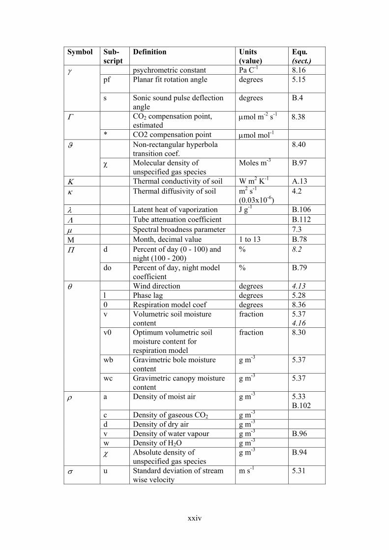
psychrometric constant Pa C-1 8.16 pf Planar fit rotation angle
degrees 5.15
γ
s Sonic sound pulse deflection angle
degrees B.4
CO2 compensation point, estimated
µmol m-2 s-1 8.38 Γ
* CO2 compensation point µmol mol-1 Non-rectangular hyperbola
transition coef. 8.40 ϑ
χ Molecular density of
unspecified gas species Moles m-3 B.97
Κ Thermal conductivity of soil W m2 K-1 A.13 κ Thermal diffusivity of soil m2 s-1
(0.03x10⁻⁶) 4.2
λ Latent heat of vaporization J g-1 B.106 Λ Tube attenuation coefficient B.112 µ Spectral broadness parameter 7.3 Μ Month, decimal value 1 to 13 B.78
d Percent of day (0 - 100) and night (100 - 200)
% 8.2 Π
do Percent of day, night model coefficient
% B.79
Wind direction degrees 4.13 l Phase lag degrees 5.28 0 Respiration model coef degrees 8.36 v Volumetric soil moisture
content fraction 5.37
4.16 v0 Optimum volumetric soil
moisture content for respiration model
fraction 8.30
wb Gravimetric bole moisture content
g m-3 5.37
θ
wc Gravimetric canopy moisture content
g m-3 5.37
a Density of moist air g m-3 5.33 B.102
c Density of gaseous CO2 g m-3 d Density of dry air g m-3 v Density of water vapour g m-3 B.96 w Density of H2O g m-3
ρ
χ Absolute density of unspecified gas species
g m-3 B.94
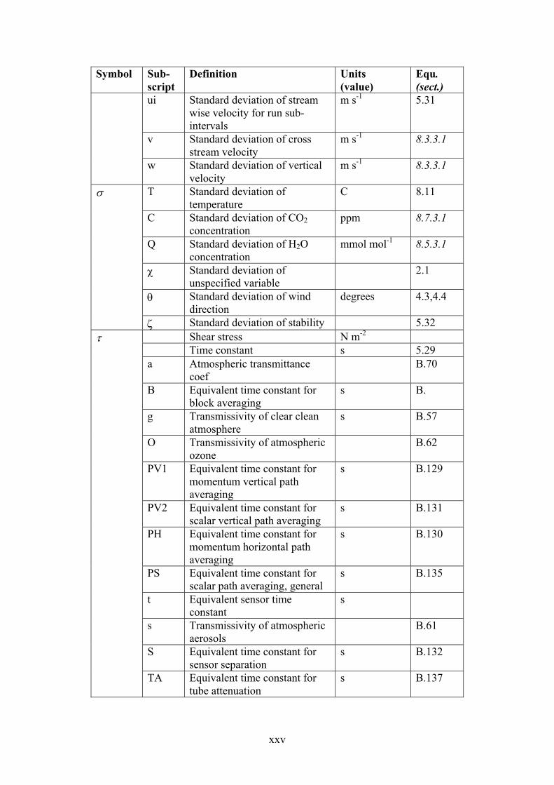
σ u Standard deviation of stream wise velocity
m s-1 5.31
xxiv
Symbol Sub-script
Definition Units (value)
Equ. (sect.)
ui Standard deviation of stream wise velocity for run sub-intervals
m s-1 5.31
v Standard deviation of cross stream velocity
m s-1 8.3.3.1
w Standard deviation of vertical velocity
m s-1 8.3.3.1
T Standard deviation of temperature
C 8.11
C Standard deviation of CO2 concentration
ppm 8.7.3.1
Q Standard deviation of H2O concentration
mmol mol-1 8.5.3.1
χ Standard deviation of unspecified variable
2.1
θ Standard deviation of wind direction
degrees 4.3,4.4
σ
ζ Standard deviation of stability 5.32 Shear stress N m-2 Time constant s 5.29 a Atmospheric transmittance
coef B.70
B Equivalent time constant for block averaging
s B.
g Transmissivity of clear clean atmosphere
s B.57
O Transmissivity of atmospheric ozone
B.62
PV1 Equivalent time constant for momentum vertical path averaging
s B.129
PV2 Equivalent time constant for scalar vertical path averaging
s B.131
PH Equivalent time constant for momentum horizontal path averaging
s B.130
PS Equivalent time constant for scalar path averaging, general
s B.135
t Equivalent sensor time constant
s
s Transmissivity of atmospheric aerosols
B.61
S Equivalent time constant for sensor separation
s B.132
τ
TA Equivalent time constant for tube attenuation
s B.137
xxv

Symbol Sub-script
Definition Units (value)
Equ. (sect.)
Cyl Equivalent time constant for cylindrical averaging
s B.136
Sph Equivalent time constant for spherical averaging
s B.138
w Transmissivity of atmospheric water vapour
B.59
υ Viscosity of air
B.117
ς Atmospheric scattering coefficient
B.70
ω i Albedo model light scattering coefficeint
B.76
Longitude degrees B.51 Ω o Time standard longitude degrees B.51
ξ Atmospheric scattering coefficient
B.71
Ξ Latitude degrees B.53 Ψ Stability adjustment function 8.9
xxvi

xxvii
Proposition 37
No improvement can take place in the Art of the present generation until all classes,
Artists, Manufacturers, and the Public, are better educated in Art, and the existence of
general principles is more fully recognised.
Proposition 13
Flowers or other natural objects should not be used as ornaments, but conventional
representations founded upon them sufficiently suggestive to convey the intended
image to the mind, without destroying the unity of the object they are employed to
decorate. Universally obeyed in the best periods of Art, equally violated when Art
declines.
Proposition 4
True beauty results from that repose which the mind feels when the eye, the intellect,
and the affections, are satisfied from the absence of any want.
Owen Jones
The Grammar of Ornament, 1856