1

Mark-to-Market: Real Effects and Social Welfare

Frank Gigler* Chandra Kanodia* Raghu Venugopalan**

Current revision: August 2016

ABSTRACT Mark-to-market (MTM) information improves welfare by facilitating external decisions. But due to feedback effects, MTM also stimulates pro-cyclical forces that make the firm’s wealth highly volatile. To counteract this increased volatility firm’s have a strong incentive to reduce their exposure to MTM adjustments by changing the asset portfolios they hold. In this paper, we assess the desirability of MTM in a setting where all of the above forces are endogenously determined. We derive the essential tradeoffs that determine the net welfare effects of MTM accounting. We show that, beyond a certain threshold, greater precision in the information provided by MTM would cause the welfare of all affected agents to decline.

* Carlson School of Management, University of Minnesota ** University of Texas, Arlington We thank Nahum Melumad, Amir Ziv, Haresh Sapra, Ron Dye, Shiva Sivaramakrishnan, Sunil Dutta, and Greg Clinch for many helpful comments on earlier versions of this paper. We have also benefited from numerous comments by seminar participants at Baruch City College, Columbia University, the University of Chicago, Northwestern University, Rice University, Southern Methodist University, University of California at Irvine, University of Toronto, Washington University in St. Louis, Rutgers Business School, the 2014 Accounting Theory Conference, the 2014 LAEF Conference at Santa Barbara, the Indian School of Business 2015 Accounting Conference and the 2016 UTS Australian Summer Accounting Conference.

2

1. Introduction The financial crises of 2007-09 ignited an important debate among professional managers,

regulators, the US Congress and academics about the economic consequences of mark-to-market

(MTM) accounting (aka, fair value accounting). Many in the professional community argued that

MTM was contributing significantly to the downward spiral in the economy.1 Many in the academic

community argued that MTM measurements were mere messengers providing timely information that

could only facilitate corrective actions.2 The debate between these two points of view is but one

example of a larger issue. Do accounting measurements and reports to external parties merely mirror

the events occurring in a firm, or could they actually contribute to those events? If the former is true

then accounting reports could never have adverse consequences; they could only facilitate welfare

improving actions by external parties. More information would always be better than less. If the latter

is true then accounting regulators like the Financial Accounting Standards Board (FASB) must

carefully balance the benefits of facilitating external decisions against the possibly adverse

transformative consequences inside the firm.

In this paper, we describe and analyze a setting which illustrates how MTM accounting

transforms the financial wealth of the firm while conveying information to external agents that is used

to assess the firm’s financial condition. We explicitly derive and analyze the tradeoff between causing

such wealth transformations and providing information to facilitate external decisions. Our analysis is

indicative of how standard setting could go awry and produce many unintended consequences when

standard setters assume (as the FASB apparently does) that firms’ operations are independent of how

they are measured and reported to outsiders. 1 For examples, see Forbes (2009), Wallision (2008a, 2008b) and Whalen (2008). Similar concerns were expressed by the American Bankers Association and in US Congressional debates. 2 See Barth, Beaver and Landsman (2001 and Barth (2006). Laux and Leuz (2009) argue that: “FVA is neither responsible for the crisis nor is it merely a measurement system that reports asset values without having economic effects of its own.”

3

As claimed by its supporters, MTM accounting certainly provides a much more accurate

picture of a firm’s current financial situation. This greater transparency enables better decisions and

actions by external agents in all situations where the payoff to those decisions is affected by the firm’s

wealth.3 But, such decisions and actions are not necessarily “corrective” of a failing situation. For

example, potential employees may be concerned with a firm’s financial health when deciding where to

seek employment. Customers may want to know that they are buying from a firm that will remain

financially viable in the future. Suppliers of raw materials and services to a firm are concerned with

the financial strength of the firm, and investors demand such information when called upon to finance

new debt or equity. In each of these situations the interaction between the firm and external agents is

not entirely one sided. The financial condition of the firm certainly affects the payoff to external

agents, but also, collectively, the actions taken by these external agents have significant effects on the

firm’s wealth. The change in the firm’s wealth is likely to be procyclical, in the sense that when the

situation looks good to external agents they take actions that make it better and a situation that doesn’t

look good could trigger a flight of financial capital, human capital, and abandonment by suppliers and

customers that make the financial condition of the firm much worse. Faced with the possibility of

such increased volatility, managers are likely to take anticipatory actions to diminish the effect of

MTM on external agents’ actions.

The interactive effects described above could be quite large. In their presence, the task of

assessing the desirability of MTM is not as simple as asking whether the information provided by

MTM is sufficiently reliable and whether outside stakeholders would want it. In most situations,

individual external agents are so small that each individual’s own actions have no measurable effect on

the firm’s financial condition. Additionally, any anticipatory actions taken by managers will be

perceived as sunk. Therefore to each individual external agent, the firm’s financial situation at the

3 This claim follows from Blackwell’s theorem.

4

time she needs to act, would indeed be a state of Nature, in which case only the decision facilitating

role of MTM would be of concern. Thus every external agent would rationally demand the kind of

information provided by MTM. But when the information is publicly provided, the actions of all

agents are affected in the same direction, in which case the collective effect on the firm’s wealth could

be highly significant. If the change in the firm’s wealth, or the anticipatory actions taken by

corporate managers, adversely affects the payoff to external agents, then providing the

information may be socially undesirable, even though each individual user of the information

would demand it. In such situations, making accounting policy by merely acceding to the

demands of external users is not the appropriate response by regulators. The social costs and

benefits of increased disclosure could be quite subtle, but can be endogenously characterized, and

regulators need to carefully assess them before arriving at an appropriate accounting policy.

The results we derive, when the firm’s wealth is allowed to endogenously adjust to accounting

measurement, are starkly different from traditional wisdom. (i) The traditional wisdom is that

information decreases uncertainty (which is always true in one sided interactions with Nature). In

contrast, we find that information provided to aid in the assessment of a firm’s wealth increases the

uncertainty in that wealth. (ii) The traditional wisdom is that, regardless of whether we mark-to-

market the assets of a firm or don’t mark them to market, the firm’s assets remain exactly the same;

only the accounting numbers change. In contrast, we find that the assets that are marked to market in

an MTM regime would be quite different from the assets that the firm would hold in historical cost

regime. (iii) Traditional wisdom suggests that the more relevant the firm’s wealth is to the decisions

of external stakeholders the more precise should be the information supplied to them. However, we

find that the greater the need of outside stakeholders to assess the firm’s wealth, the less precise

should be the fair value information that is provided to them. In terms of ex ante welfare, we find that

5

the firm (i.e. its shareholders) would unambiguously prefer historical cost to fair value accounting. We

identify plausible conditions under which even outside stakeholders are worse off from fair value

accounting. We find that there is a time inconsistency problem in determining disclosure policy that is

analogous to the well-known time inconsistency of optimal monetary and government policy (Kydland

and Prescott, 1977). At the time that outside stakeholders need to make their decisions they would

demand the most precise fair value information that is feasible, but from an ex ante perspective such a

disclosure policy could actually make them worse off.

Our results cast doubt on the desirability of fair value accounting and, more generally, on the

wisdom of making accounting policy under the assumption that accounting information is analogous

to information about the state of Nature. Plantin, Sapra and Shin (2008) and Allen and Carletti (2008)

have also raised concerns about fair value accounting and have identified some of its negative

consequences. However, in this previous research the concerns originate from measurement

difficulties when there is a lack of liquidity in the market for the firm’s assets. Our analysis does not

depend on measurement difficulties and liquidity issues and challenges a pervasive assumption

underlying the determination of accounting standards in general.

The wealth transformation effect of MTM accounting is a special case of the “real effects” of

financial markets that have been studied in many different contexts, both theoretically and empirically.

One strand of this literature argues that real effects arise due to the information transmission role of

prices in financial markets when traders and speculators in the market are collectively better informed

than corporate managers. Bond, Edmans and Goldstein (2012) provide a comprehensive survey of this

research. A second strand, concerned with the real effects of accounting measurement, assumes that a

priori corporate managers possess information that markets do not have. In this second strand, a

manager’s incentive to choose among various courses of action depends upon how prices in financial

markets respond to these actions. Price response, in turn, depends upon the information in the capital

6

market as augmented by the information contained in accounting measurements. For example, in

Kanodia, Sapra and Venugopalan (2004), a firm’s incentive to invest in intangible assets depends upon

the observability of such investments by investors in the capital market which, in turn, depends at least

partially upon the accounting treatment of intangible assets. A general discussion and survey of this

literature is contained in Kanodia (2006) and Kanodia and Sapra (2016). In the current paper, we do

not model capital markets, so the real effects we study here are not price mediated. Instead, we model

a setting where the payoff to actions taken by external agents, like the firm’s customers or the firm’s

suppliers, depends directly upon the financial strength of the firm. These external agents, therefore,

demand and use accounting reports based on MTM measurements to assess the financial state of the

firm and these assessments guide their actions. Collectively, these actions feed into the firm’s

financial performance and wealth. This approach allows us to succinctly capture both the decision

facilitating role and the wealth transformation effects of accounting information.

The remainder of this paper is organized as follows. Section 2 describes the economic setting

that we analyze and sections 3 and 4 derive the equilibrium for the setting by working backwards from

later actions to earlier actions. Section 3 derives the equilibrium behavior of external agents who use

the information provided by MTM accounting and act after this information is released. Section 4

characterizes the equilibrium actions of the firm taken in anticipation of the equilibrium response of

external agents to the release of MTM information. Section 5 contains a welfare analysis of the

equilibrium and develops the tradeoffs, suggested by our model, that regulators should consider in

assessing the desirability of MTM accounting. Section 6 concludes.

2. The Economic Setting

There are three dates, 0,1 and 2. Date 0 is an initial date, date 1 is an interim date, and date 2

is the final date. At the initial date, the firm chooses a portfolio of assets to hold. These assets change

7

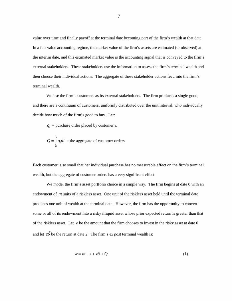
value over time and finally payoff at the terminal date becoming part of the firm’s wealth at that date.

In a fair value accounting regime, the market value of the firm’s assets are estimated (or observed) at

the interim date, and this estimated market value is the accounting signal that is conveyed to the firm’s

external stakeholders. These stakeholders use the information to assess the firm’s terminal wealth and

then choose their individual actions. The aggregate of these stakeholder actions feed into the firm’s

terminal wealth.

We use the firm’s customers as its external stakeholders. The firm produces a single good,

and there are a continuum of customers, uniformly distributed over the unit interval, who individually

decide how much of the firm’s good to buy. Let:

iq = purchase order placed by customer i.

1

0iQ q di= ∫ = the aggregate of customer orders.

Each customer is so small that her individual purchase has no measurable effect on the firm’s terminal

wealth, but the aggregate of customer orders has a very significant effect.

We model the firm’s asset portfolio choice in a simple way. The firm begins at date 0 with an

endowment of m units of a riskless asset. One unit of the riskless asset held until the terminal date

produces one unit of wealth at the terminal date. However, the firm has the opportunity to convert

some or all of its endowment into a risky illiquid asset whose prior expected return is greater than that

of the riskless asset. Let z be the amount that the firm chooses to invest in the risky asset at date 0

and let zθ be the return at date 2. The firm’s ex post terminal wealth is:

w m z z Qθ= − + + (1)

8

Thus, the firm’s terminal wealth depends partly upon a decision made by the firm’s inside

manager and partly upon the aggregate of decisions made by a continuum of outside

stakeholders. These decisions are made sequentially. The inside decision is made prior to the

realization of the fair value signal, while external decisions are made after receipt of the fair

value signal.

We assume that except for informational differences, all customers are identical. The

payoff to a customer for ordering from our incumbent firm depends partly upon a known

parameter η that describes how well the characteristics of the good produced by the firm match

the needs of its customers, and partly upon the financial strength of the firm. The ex post payoff

to a customer who places an order of size iq is:

212i i iu Aq q= − (2)

where 212 iq can be interpreted as the cost of using the good in whatever manner the customer

uses it4. The marginal benefit to a customer from purchasing its needs from the incumbent firm

is described by:

(1 )A wτη τ≡ + − ,

where 0 (1 ) 1τ< − < describes the relative extent to which customers are affected by the

financial strength of the firm that supplies them5. Customers make their purchase decisions

4 The model of customers used here is a variation on the model of individual investment decisions with strategic complementarities in Angeletos and Pavan (2004). 5 That customers are reluctant to place orders with suppliers who are perceived to be financially weak, is a well known empirical phenomenon. General Motors was faced with this predicament during the recent financial crisis. A possible reason for this phenomenon is that the benefit to a customer from today’s purchase depends partially upon future supplies of goods and services by the incumbent supplier, and the supplier’s ability to perform in the future is affected by his current financial strength. Another possibility is that firms that are

9

after receiving the fair value signal provided by the accounting system. The fair value of the

risky asset at this interim date provides noisy information about its terminal value and therefore

the fair value signal is incrementally informative about the terminal wealth of the firm.

3. Customers’ Purchase Decisions

Let ( )iE A be customer 'i s expectation of A conditional on the information she receives

at date 1. Then, the order placed by customer i is the unique solution to:

21( )2iq i i iMax E A q q− (3)

The first order condition to (3) yields:

( ) (1 )[ ( ) ( )]i i i iq E A m z zE E Qτη τ θ= = + − − + + (4)

The presence of ( )iE Q in the first order condition for iq implies the presence of strategic

complementarities in customer purchase decisions. The marginal benefit to purchasing from the

firm is higher the higher the quantity that other customers purchase from the firm.

Expectations of θ are determined by standard Bayesian updating of the prior

distribution of θ . But expectations of the aggregate order Q are a much more complex object.

These latter expectations depend upon what customer i thinks other customers will do, and

therefore on i’s beliefs of the beliefs of other customers and i’s beliefs of other customers’ beliefs

of other customers beliefs, and so on. As is standard in the literature on higher order beliefs,

struggling financially may be motivated to cut corners and sacrifice attributes of the good that are not readily visible to customers.

10

( )iE Q is calculated iteratively, and is described by an infinite hierarchy of higher order beliefs

of θ . We construct this hierarchy below.

Since 1

0iQ q di= ∫ , it follows from the first order condition (4) that:

1 1

0 0

(1 )( ) (1 ) ( ) (1 ) ( )i iQ m z z E di E Q diτη τ τ θ τ= + − − + − + −∫ ∫ (5)

We refer to ( )iE θ as the first order belief of customer ,i and 1

0

( )iE diθ∫ as the average first

order belief about θ in the population of customers. No customer knows what this average

belief is, but each customer can form a belief of this average belief which I denote by

1

0

( )i jE E djθ∫ . From (5),

1 1

0 0

( ) (1 )( ) (1 ) ( ) (1 ) ( )i i j i jE Q m z zE E dj E E Q djτη τ τ θ τ= + − − + − + −∫ ∫ (6)

In (6) the expression 1

0

( )i jE E Q dj∫ is conceptually well defined since it is customer 'i s belief of

the average belief of Q in the customer population, but we don’t yet know how to calculate it.

Inserting (6) into the customer’s first order condition yields:

2

1 12 2

0 0

(1 )( ) (1 ) ( ) (1 ) (1 ) ( )

(1 ) ( ) (1 ) ( )

i i

i j i j

q m z zE m z

zE E dj E E Q dj

τη τ τ θ τ τη τ

τ θ τ

= + − − + − + − + − − +

− + −∫ ∫

(7)

11

Integrating the expression in (7) over the customer population yields:

12

01 1 1 1

2 2

0 0 0 0

(1 )( ) (1 ) ( ) (1 ) (1 ) ( )

(1 ) ( ) (1 ) ( )

i

i j i j

Q m z z E di m z

z E E djdi E E Q djdi

τη τ τ θ τ τη τ

τ θ τ

= + − − + − + − + − − +

− + −

∫

∫ ∫ ∫ ∫

(8)

In (8) the expression ( )i jE E djdiθ∫ ∫ is the average expectation of the average expectation of θ

in the customer population. We refer to it as the average second order expectation of .θ Now,

(8) can be used to obtain an updated calculation of ( )iE Q and this updated expression for

( )iE Q can be inserted into the customer’s first order condition (4) to yield an updated

expression for .iq Integrating this updated expression for iq yields the following updated

expression for the aggregate order quantity .Q

2 2 3

1 1 12

0 0 01 1 1 1 1 1

3 3

0 0 0 0 0 0

(1 ) (1 ) (1 )( ) (1 ) ( ) (1 ) ( )

(1 ) ( ) (1 ) ( )

(1 ) ( ) (1 ) ( )

i i j

i k j i k j

Q m z m z m z

z E di z E E djdi

z E E E djdkdi E E E Q djdkdi

τη τ τη τ τη τ τ τ

τ θ τ θ

τ θ τ

= + − + − + − − + − − + − − +

− + − +

− + −

∫ ∫ ∫

∫ ∫ ∫ ∫ ∫ ∫

(9)

Comparing (5), (8), and (9) it is clear that repeated iteration yields:

2

2

(1) (2) 2 (3)

[1 (1 ) (1 ) ........](1 )( )[1 (1 ) (1 ) ........](1 ) [ (1 ) (1 ) ...........]

Qm z

z

τη τ τ

τ τ τ

τ θ τ θ τ θ

= + − + − + +

− − + − + − + +

− + − + − +

(10)

12

where, ( ) , t 1, 2,3,.....tθ = denotes the average t th. order expectation of θ . Since 0 (1 ) 1τ< − < ,

each of the infinite series contained in (10) is convergent and well defined. Carrying out the

summation yields the final expression:

( 1)(1 )( ) (1 ) (1 )t t

t o

m zQ zτη τ τ τ θτ

∞+

=

+ − −= + − −∑ (11)

Notice from (11) that the undefined expectations of Q have vanished and have been replaced by

well defined higher order expectations of .θ

We assume that the information structure in the economy is as follows. The commonly

known prior distribution of θ is Normal with mean 1 and variance .µa

Equivalently,

1, (0, ).Nθ µ ξ ξa

= + We assume 1µ > so that investment in the risky asset is a priori

desirable. Both historical cost accounting and fair value accounting reveal the amount z of

investment in the risky asset but, at date 1, fair value accounting provides an additional signal

that is not provided by historical cost accounting. Fair value accounting provides an estimate of

the date 1 value of the risky asset. We assume that the fair value estimate at the interim date is a

noisy version of its terminal value, which is zθ . Since z is known, we can model the fair value

signal as:

1, (0, )y Nθ ε εβ

= +

13

Higher values of β represent more precise measurement, and the lowest value of β , i.e. 0β =

is equivalent to not providing any fair value information. Therefore 0β = is representative of

historical cost accounting. In addition to the public fair value signal, customers may have

private sources of information about the return to the risky asset. We model this as private

unbiased signals, ix , with some common precision γ :

1, (0, )i i ix Nθ ω ωγ

= +

We think that a setting with both public and private information is interesting in its own right, as

it captures the realistic idea that in the absence of a public source of information, individual

agents will have idiosyncratic beliefs regarding uncertain variables.6 We assume that all of the

noise terms, , , and iξ ε ω are independent of each other and independent of .θ

We now proceed to derive the equilibrium aggregate order quantity Q and individual

beliefs ( )iE Q for the specific information structure described above. The first order belief of

customer i is:

( ) ii

y xE aµ β γθa β γ+ +

=+ +

(12)

It is convenient to rewrite the above expression in a different way. Let

6 There is also a technical motivation for introducing private signals. A game with strategic complementarity and homogenous beliefs generally has multiple equilibria. As shown by Carlsson and Van Damme (1993), the introduction of private information gets rid of the multiplicity and produces a unique equilibrium. Additionally, the limiting unique equilibrium as the precision of the private signal goes to zero, is commonly used as predictive of what would be observed in settings with only public information. Heinemann, Nagel and Ockenfels (2004) provide empirical support for this latter claim.

14

γδ

a β γ≡

+ +, and

yP aµ β

a β+

≡+

Then (12) is equivalent to:

( ) (1 )i iE x Pθ δ δ= + − , (13)

where P can be thought of as the public information in the economy and ix as the private

information of customer .i The average first order belief of θ is:

( )(1) ( ) (1 ) (1 )i iE di x P di Pθ θ δ δ δθ δ≡ = + − = + −∫ ∫ ,

from which it follows that 'i s belief of the average first order belief is:

( ) ( ) (1 )i j iE E dj E Pθ δ θ δ= + −∫

= [ (1 ) ] (1 )ix P Pδ δ δ δ+ − + −

= 2 2(1 )ix Pδ δ+ −

Therefore the average second order belief of θ is:

(2) 2 2( ) (1 )i jE E djdi Pθ θ δ θ δ≡ = + −∫ ∫

15

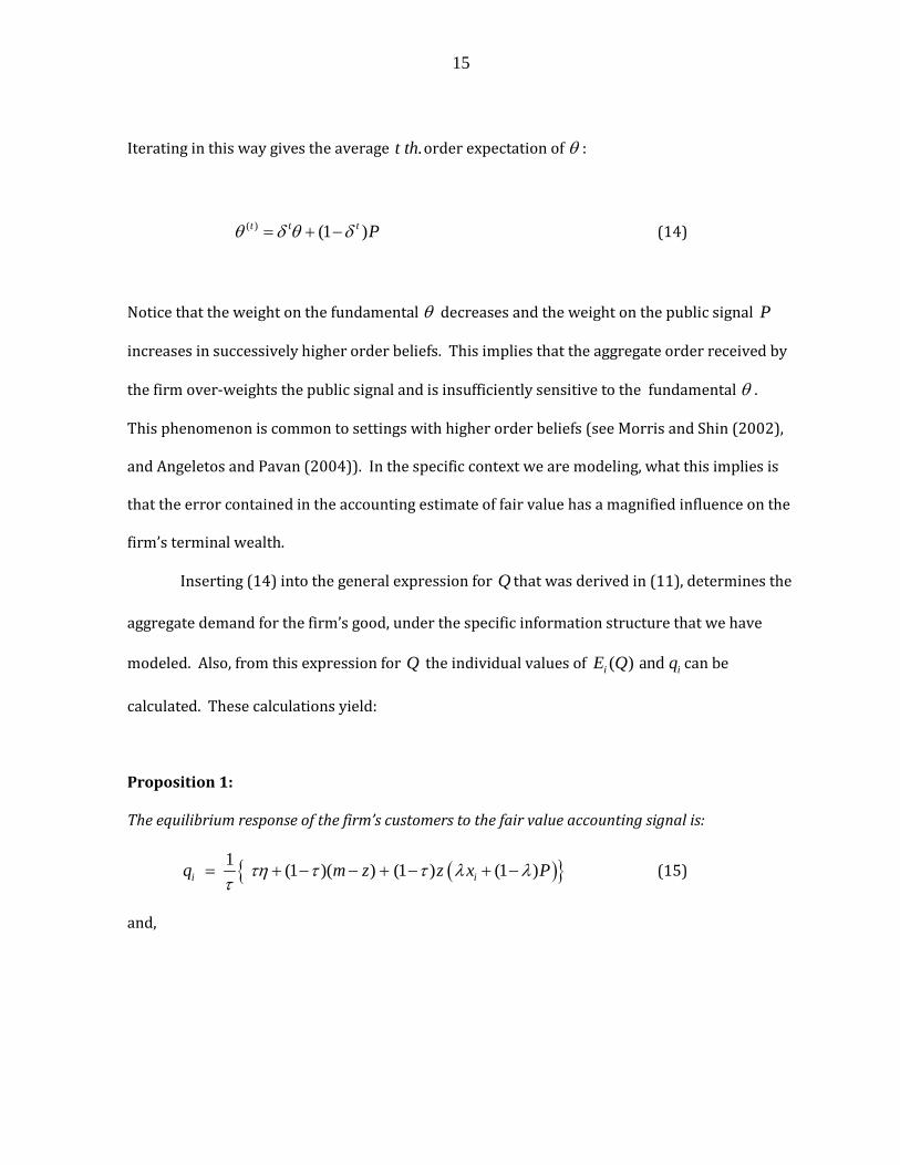
Iterating in this way gives the average .t th order expectation of θ :

( ) (1 )t t t Pθ δ θ δ= + − (14)

Notice that the weight on the fundamental θ decreases and the weight on the public signal P

increases in successively higher order beliefs. This implies that the aggregate order received by

the firm over-weights the public signal and is insufficiently sensitive to the fundamental θ .

This phenomenon is common to settings with higher order beliefs (see Morris and Shin (2002),

and Angeletos and Pavan (2004)). In the specific context we are modeling, what this implies is

that the error contained in the accounting estimate of fair value has a magnified influence on the

firm’s terminal wealth.

Inserting (14) into the general expression for Q that was derived in (11), determines the

aggregate demand for the firm’s good, under the specific information structure that we have

modeled. Also, from this expression for Q the individual values of ( ) and i iE Q q can be

calculated. These calculations yield:

Proposition 1:

The equilibrium response of the firm’s customers to the fair value accounting signal is:

( ) 1 (1 )( ) (1 ) (1 )i iq m z z x Pτη τ τ λ λτ

= + − − + − + − (15)

and,

16

( ) 1 (1 )( ) (1 ) (1 )Q m z z Pτη τ τ λθ λτ

= + − − + − + − (16)

where,

1 (1 )

τδλτ δ

≡− −

Proof: See the Appendix.

Because 1, 0, 11 (1 )

τ δ ττ δ

< ∀ > < − −

, the equilibrium weight on

in (15) and on in (16)ix θ is strictly less than δ , which is the weight that would be used in

Bayesian updating. This confirms the earlier intuition that, because of the need to assess the

beliefs of others, each individual customer under-weights his private information about θ and

over-weights the public information in deciding how much to order from the firm. In turn, this

results in the equilibrium aggregate order quantity Q becoming less sensitive to fluctuations in

the fundamentals θ and overly sensitive to the public information provided by fair value

accounting. The effect of this distortion on social welfare will be developed in a later section.

4. The Firm’s Asset Allocation Decision:

We now turn to the firm’s asset portfolio choice to be made at date 0. As specified

earlier, the firm’s terminal wealth is w m z z Qθ= − + + . We assume the firm is risk averse with

constant absolute risk aversion 0ρ > . If w is distributed Normal, as will be the case, the firm’s

objective function is:

17

1( ) ( )2zMax E w Var wρ −

(17)

From the perspective of date 0, the aggregate order received by the firm at date 1 is a random

variable because individual customer orders depend upon the public fair value signal and the

private signals that customers receive at date 1. At date 0 these signals are random variables.

The equilibrium value of Q , as determined in (16), is distributed Normal since it depends

linearly on the Normally distributed return θ as well as on the Normally distributed fair value

report y that is released later at date 1.

Using the facts that ( ) ( ) ,E P E θ µ= = we obtain from (16):

(1 )[ ( 1)]( ) m zE Q τη τ µ

τ+ − + −

= (18)

and,

( 1)( ) ( 1) ( ) m zE w m z E Q τη µµ

τ+ + −

= + − + = (19)

The firm’s investment in the risky asset affects its expected terminal wealth in two ways.

There is a direct effect and an indirect effect. Since 1µ > , the direct effect of increased

investment in the risky asset is to increase the expected net return on this asset. The indirect

effect operates through the firm’s customers. A customer’s response to the firm’s investment in

the risky asset depends upon both the private signal and the public fair value signal she receives

at date 1. Unfavorable signals decrease a customer’s demand and favorable signals increase her

18

demand. The private signals received by customers affect individual demands but not the

aggregate demand that feeds into the firm’s wealth. This is because variations in private signals

are independent over the customer population and so cancel out in the aggregate. However, the

public fair value signal is perfectly correlated across customers, so its effect on customer

demand is like a systematic shock that persists over the customer population. If the fair value

signal is favorable, then the firm’s investment in the risky asset increases aggregate customer

demand for the firm’s good, but if the fair value signal turns out to be unfavorable then aggregate

demand is decreasing in the risky investment. Since the fair value signal is unbiased, the news is

expected to be neutral, and neutral news is good news because 1.µ > So, in expectation,

aggregate customer demand for the firm’s good is increasing in the amount invested in the risky

asset.

But, the fair value signal also induces volatility in the aggregate demand for the firm’s

good and this volatility is increasing in the amount invested in the risky asset. Below, we

characterize the risk in the firm’s terminal wealth from a date 0 perspective.

2( ) ( ) var( ) 2 cov( , )var w z var Q z Qθ θ= + + (20)

The first term in (20), 2 ( ),z var θ captures the direct effect of higher investment in the risky asset on

the risk in the firm’s wealth. The second and third terms derive from customer assessments of the

firm’s wealth and the consequent change in their order decisions due to observation of the fair value

signal. We assess (20) term by term.

1var( ) var( )θ ξa

= =

From (16):

19

2

21var( ) var[ (1 ) ]Q z Pτ λθ λτ− = + −

= 2

2 2 21 [ var( ) (1 ) var( ) 2 (1 )cov( , )]z P Pτ λ θ λ λ λ θτ− + − + −

(21)

where,

2

2

var( ) var( )

1 1 1

P yβa β

β βa β a β a β a

= +

= + = + +

and,

cov( , ) cov ,

1var( )

P yβθ θa β

β βθa β a β a

= +

= = + +

Inserting these last two calculations into (21) gives:

22 2 21 1var( ) (1 ) 2 (1 )Q zτ β βλ λ λ λ

τ a a β a β − = + − + − + +

which simplifies to:

2

2 2 21 1var( ) (1 )Q zτ βλ λτ a a β

− = + − + (22)

Lemma 1:

20

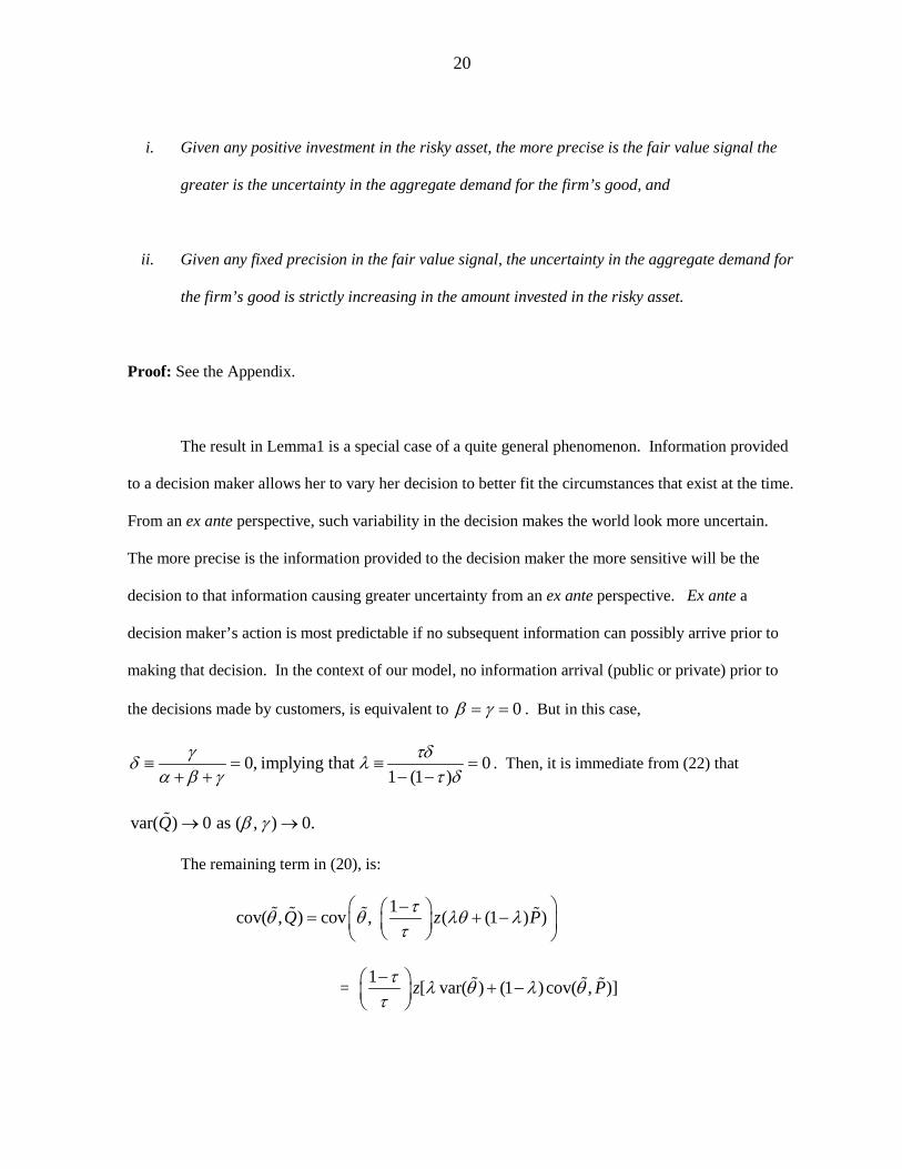
i. Given any positive investment in the risky asset, the more precise is the fair value signal the

greater is the uncertainty in the aggregate demand for the firm’s good, and

ii. Given any fixed precision in the fair value signal, the uncertainty in the aggregate demand for

the firm’s good is strictly increasing in the amount invested in the risky asset.

Proof: See the Appendix.

The result in Lemma1 is a special case of a quite general phenomenon. Information provided

to a decision maker allows her to vary her decision to better fit the circumstances that exist at the time.

From an ex ante perspective, such variability in the decision makes the world look more uncertain.

The more precise is the information provided to the decision maker the more sensitive will be the

decision to that information causing greater uncertainty from an ex ante perspective. Ex ante a

decision maker’s action is most predictable if no subsequent information can possibly arrive prior to

making that decision. In the context of our model, no information arrival (public or private) prior to

the decisions made by customers, is equivalent to 0β γ= = . But in this case,

0, implying that 01 (1 )

γ τδδ λa β γ τ δ

≡ = ≡ =+ + − −

. Then, it is immediate from (22) that

var( ) 0 as ( , ) 0.Q β γ→ →

The remaining term in (20), is:

1cov( , ) cov , ( (1 ) )Q z Pτθ θ λθ λτ

− = + −

= 1 [ var( ) (1 )cov( , )]z Pτ λ θ λ θτ− + −

21

= 1 1 (1 )zτ βλ λτ a a β

− + − + (23)

which is also strictly increasing in .β

Inserting (22) and (23) into (20) gives:

22 2 2 2

2

1 1 1var( ) (1 )

1 12 (1 )

w z z

z

τ βλ λa a τ a β

τ βλ λa τ a β

− = + + − + + − + − +

(24)

Proposition 2:

Keeping fixed the firm’s investment in the risky asset, the more precise is the fair value information

provided to outside stakeholders to assist in assessing the firm’s wealth the more uncertain the wealth

of the firm becomes from an ex ante perspective.

Proof: See the Appendix.

Proposition 2 is a stark departure from traditional wisdom, since in most economic models the

arrival of information decreases uncertainty. But, it is important to ask from whose perspective are we

assessing the uncertainty in the environment. It is certainly true that information provided at date 1

decreases the uncertainty faced by economic agents who make decisions at date1. But, what happens

to the uncertainty faced by economic agents who must move earlier, before the information is

provided? Given that the decision made by later economic agents is sensitive to the information

22

provided to them, the earlier economic agents must perceive the decisions made by the later economic

agents as random variables and therefore the information actually increases the uncertainty they face.

Proposition 2 is also indicative of how misleading accounting disclosure studies could be when the

variable of interest is assigned an exogenously specified distribution. In such studies information

always reduces uncertainty, since statistically a conditional variance is smaller than an unconditional

variance. In our study too, if the firm’s wealth is an exogenously given random variable then

information used to assess the firm’s wealth can only decrease the uncertainty in wealth. But such a

scenario is an over-simplification of the real world. Realistically, a firm’s wealth depends not just

upon the state of Nature, but also upon decisions made by both insiders and outsiders. If the

disclosure of information alters the decisions of outsiders and if these decisions affect the distribution

of the firm’s wealth then it is not necessarily true that information is uncertainty reducing.

We can now characterize the firm’s date 0 investment in the risky asset. Inserting (19) and

(24) into the firm’s objective function, as described in (17), and differentiating with respect to z gives

the first order condition:

22 2

1

1 1 11 (1 ) 2 (1 )z µ

τ β τ βτρ λ λ λ λa τ a β τ a β

−=

− − + + − + + − + +

(25)

Equation (25) indicates that the firm is not passive to the provision of fair value information.

The firm chooses its asset portfolio anticipating the revaluation that occurs at subsequent dates and the

effect such revaluations have on the decisions of outsiders. To see the effect of fair value information

on the firm’s asset choices let us examine how variations in β affect the firm’s choice of z . From

23

(25) it is clear that the effect of on zβ is through the two factors 2 2(1 ) βλ λa β

+ − + and

(1 ) βλ λa β

+ − + contained in the denominator of (25). In the proofs of Lemma 1 and

Proposition 2, we established that both factors are strictly increasing in .β Therefore, the

denominator in (25) is strictly increasing in , implying that 0zββ∂

<∂

. Noting that 0β = is

representative of historical cost, we have:

Proposition 3

i. The firm holds a different portfolio of assets in a fair value accounting regime than it would

hold in a historical cost regime.

ii. Fair value accounting causes the firm to shift away from assets whose fair values are more

volatile and invest more in assets whose fair values are stable.

iii. The more precise is the fair value information the greater the shift in the firm’s asset portfolio.

The result described in Proposition 3 is due to the fact that the precision of the fair value

information increases not only the prior uncertainty in the aggregate order Q but also increases the

marginal effect of z on this uncertainty. The firm decreases its holdings of risky assets in order to

decrease the uncertainty in customer orders.

Proposition 3 is an important testable real effect of fair value accounting. It is noteworthy that

corporate managers argued against fair value accounting on the grounds that such accounting

treatment would increase the volatility of reported income. In order to understand preferences over

accounting reports one must derive them from more primitive preferences over real objects. We have

24

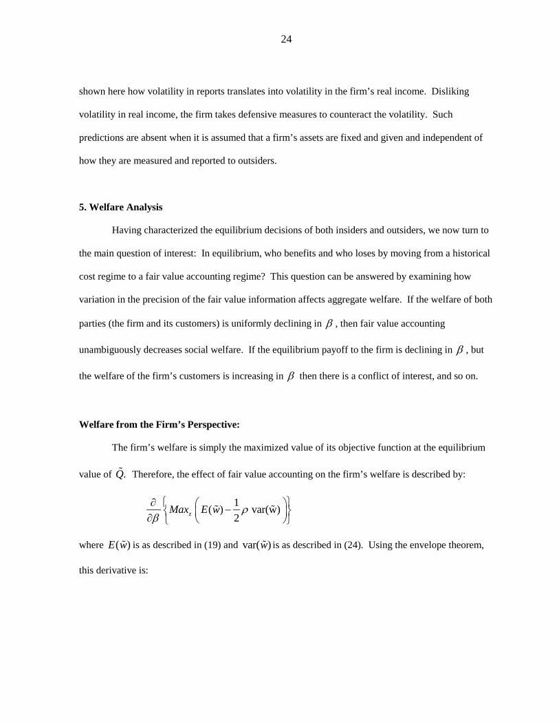
shown here how volatility in reports translates into volatility in the firm’s real income. Disliking

volatility in real income, the firm takes defensive measures to counteract the volatility. Such

predictions are absent when it is assumed that a firm’s assets are fixed and given and independent of

how they are measured and reported to outsiders.

5. Welfare Analysis Having characterized the equilibrium decisions of both insiders and outsiders, we now turn to

the main question of interest: In equilibrium, who benefits and who loses by moving from a historical

cost regime to a fair value accounting regime? This question can be answered by examining how

variation in the precision of the fair value information affects aggregate welfare. If the welfare of both

parties (the firm and its customers) is uniformly declining in β , then fair value accounting

unambiguously decreases social welfare. If the equilibrium payoff to the firm is declining in β , but

the welfare of the firm’s customers is increasing in β then there is a conflict of interest, and so on.

Welfare from the Firm’s Perspective:

The firm’s welfare is simply the maximized value of its objective function at the equilibrium

value of .Q Therefore, the effect of fair value accounting on the firm’s welfare is described by:

1( ) var(w)2zMax E w ρ

β∂ − ∂

where ( )E w is as described in (19) and var( )w is as described in (24). Using the envelope theorem,

this derivative is:

25

22 2 2 21 1 1 1 1(1 ) 2 (1 )

2z zτ β τ βρ λ λ λ λa τ β a β a τ β a β

− ∂ − ∂ − + − + + − ∂ + ∂ +

We have previously established in the proofs of Lemma 1 and Proposition 2 that both

2 2(1 ) βλ λa β

+ − + and (1 ) βλ λ

a β

+ − + are strictly increasing in .β Therefore the firm’s

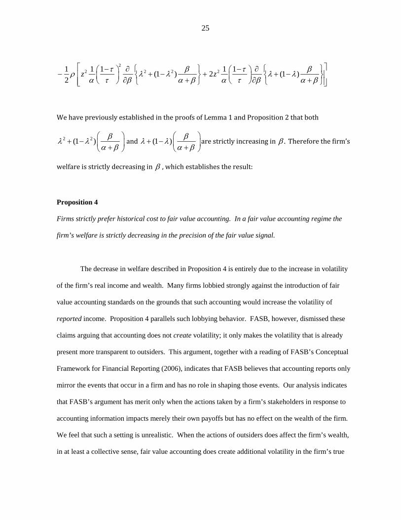
welfare is strictly decreasing in β , which establishes the result:

Proposition 4

Firms strictly prefer historical cost to fair value accounting. In a fair value accounting regime the

firm’s welfare is strictly decreasing in the precision of the fair value signal.

The decrease in welfare described in Proposition 4 is entirely due to the increase in volatility

of the firm’s real income and wealth. Many firms lobbied strongly against the introduction of fair

value accounting standards on the grounds that such accounting would increase the volatility of

reported income. Proposition 4 parallels such lobbying behavior. FASB, however, dismissed these

claims arguing that accounting does not create volatility; it only makes the volatility that is already

present more transparent to outsiders. This argument, together with a reading of FASB’s Conceptual

Framework for Financial Reporting (2006), indicates that FASB believes that accounting reports only

mirror the events that occur in a firm and has no role in shaping those events. Our analysis indicates

that FASB’s argument has merit only when the actions taken by a firm’s stakeholders in response to

accounting information impacts merely their own payoffs but has no effect on the wealth of the firm.

We feel that such a setting is unrealistic. When the actions of outsiders does affect the firm’s wealth,

in at least a collective sense, fair value accounting does create additional volatility in the firm’s true

26

income (not merely reported income), and this increased volatility does have negative economic

consequences.

Welfare from Customers’ Perspective:

We now examine the effect of fair value accounting on the ex ante social welfare of the firm’s

customers. As in Angeletos and Pavan (2004), we define the ex post social welfare Ω of the customer

population as the aggregate of their individual ex post payoffs, i.e.,

212i i iu di A q di q diΩ ≡ = −∫ ∫ ∫

We decompose this aggregate welfare in the same manner as Angeletos and Pavan (2004).

Substituting iq di Q=∫ , 2iq di∫ = 2 2( )iq Q di Q − + ∫ , and inserting the expression for A gives:

[ ] 2 21 1(1 )( ) (1 ) ( )2 2 im z z Q Q Q q Q diτη τ θ τΩ = + − − + + − − − −∫ ,

or, equivalently,

[ ] 2 21 1(1 )( ) (2 1) ( )2 2 im z z Q Q q Q diτη τ θ τΩ = + − − + − − − −∫ (26)

The expression 2( )iq Q di−∫ in (26) indicates that social welfare is enhanced if individual customer

purchases are coordinated so that each customer orders exactly the same amount, i.e. if ,iq Q i= ∀ .

This social benefit to coordination is due to the convexity in the cost function of individual customers.

If the public fair value signal is the only information available to the firm’s customers then customers

would be perfectly coordinated and the last term in (26) would disappear. However, the presence of

private information prevents such perfect coordination. In what follows, we assume, as in Angeletos

and Pavan (2004), that the weight that customers put on the financial wealth of the firm is not too

27

large, specifically, 1(2 1) 0, i.e., (1 ) .2

τ τ− > − < This ensures that when individual orders are

perfectly coordinated, aggregate customer welfare is not increasing in unbounded fashion with Q .

In order to facilitate interpretation, it is useful to first calculate customer welfare if the

information that customers receive perfectly reveals the value of θ to all of them. This is equivalent

to having β →∞ . In this case:

(1 )( ) (1 ) ,iq A m z z Q iτη τ θ τ= = + − − + + − ∀

implying:

[ ]1 (1 )( ) ,iq Q m z z iτη τ θτ

= = + − − + ∀

Therefore, from (26):

[ ] [ ]

[ ]

2 22

22

1 1 1( | perfect information) = (1 )( ) (2 1) (1 )( )2

1 (1 )( )2

z m z z m z z

m z z

τη τ θ τ τη τ θτ τ

τη τ θτ

Ω + − − + − − + − − +

= + − − +

The ex ante welfare of the customer group conditional on perfect information is the expectation of the

above expression with respect to θ :

( )

22

2

1( | , perfect information) = [ (1 )( )]21 var (1 )( )

2

E z E m z z

m z z

τη τ θτ

τη τ θτ

Ω + − − + +

+ − − +

2 2 22 2

1 1 1[ (1 )( )] (1 )2 2

m z z zτη τ µ ττ τ a

= + − − + + − (27)

The first term in (27) is the expected welfare of customers in a regime where there is no incremental

information (private or public) about the return to the risky asset, and the second term is the gain in

28

expected welfare due to perfect information. The gain is due to the fact that information allows

customers to better fit their real decisions to the true wealth of the firm. Because of the quadratic

nature of aggregate payoffs to customers, the amount of the gain is proportional to the extent of

uncertainty reduction caused by the information.

Now, consider the case of noisy public and private information. Then, working with

and iq Q as described in (15) and (16), we obtain:

Proposition 5:

[ ]22

2 22 2

1( | , noisy public and private information) (1 )( )2

1 1 1 (1 )(1 )2 ( ) ( )

E z m z z

z

τη τ µτ

τγ τττ a a β τγ a β τγ

Ω = + − − +

−+ − − − + + + +

(28)

Proof: See the Appendix

As before, the first term in (28) is expected customer welfare in the absence of any

incremental information, while the second term is the change in customer welfare brought about by

noisy public and private information. Holding z fixed, the change in customer welfare is strictly

positive, as shown below, even though the information is noisy and even though the private

component of information results in coordination losses.

2

1 1 (1 ) 1 1 (1 )( ) ( )τγ τ τγ τ

a a β τγ a β τγ a a β τγ a a β τγ− −

− − > − −+ + + + + + + +

2 1 0β τ γ

a β τγ a +

= > + + (29)

29

The overweighting of public information caused by higher order beliefs makes the gain from fair value

accounting smaller than it would otherwise be. To see this, compare (28) to (27). When the public fair

value information is infinitely precise, as in (27), private information becomes redundant so there is no

overweighting of public information. In this case the gain from fair value accounting is proportional

to 1var( )θa

= since this is the amount of uncertainty eliminated by the information that is being

provided. With noisy public and private information the residual uncertainty after providing

information is 1var( | , )ix yθ

a β γ=

+ + , so that the uncertainty eliminated by the information

provided is 1 1a a β γ−

+ + . But, the benefit from fair value information is proportional to:

2

1 1 (1 )( )τγ τ

a a β τγ a β τγ<

−− + + + + +

1 1a a β γ−

+ + because,

2

2

2

1 1 (1 )( )

( ) ( )( ) (1 )( ) 0( )( )

τγ τa β γ a β τγ a β τγ

a β τγ a β τγ a β γ τγ τ a β γa β γ a β τγ

−− − =

+ + + + + +

+ + − + + + + − − + +<

+ + + +

The full benefit from uncertainty reduction is not obtained precisely because public information is

over-weighted and private information is under-weighted.

The following result is immediate from (28):

Proposition 6: If the firm’s asset portfolio remains fixed, customer welfare is strictly increasing in

the precision of fair value information.

30

Proposition 6 succinctly captures FASB’s argument in support of fair value accounting, viz., fair value

information is relevant to external users of accounting statements and improves their decisions. If

asked at the time they choose their decisions, each of our customers would express a positive demand

for fair value accounting and would want the information to be as precise as possible. This is not

surprising. At the time that a customer needs to act, she would view the firm’s assets as sunk and the

size of the collective order quantity Q as an exogenous variable that is beyond her control. Therefore,

from the perspective of each individual customer, at date 1, the wealth of the firm is like a state of

Nature and Blackwell’s theorem would apply.

It is tempting for accounting regulators, charged with maximizing the welfare of external

users, to accede to their sequentially rational demands. But, the larger wisdom requires regulators to

take an ex ante perspective, and from such a perspective the firm’s assets cannot be viewed as fixed

and sunk. In Proposition 3, we established that the firm anticipates the increased volatility caused by

the fair valuing of its assets at a later date, and counters the increased volatility by shifting its portfolio

away from the risky asset. The more precise is the fair value information the greater the shift in the

firm’s asset portfolio. So the welfare result described in Proposition 6, while true in a partial

equilibrium sense, may no longer be true when the decline in z is taken into account. Given that

1µ > , customer welfare is strictly increasing in z as can be seen from visual inspection of (28) and

the inequality in (29). Therefore, from an ex ante perspective, an increase in the precision of the fair

value signal generates two opposing effects: It enables better decisions which increase customer

welfare, but it also causes lower investment in the risky asset which decreases customer welfare.

Whether or not customers are better off, in an overall sense, depends on which of these two effects

dominate. Below, we investigate the net effect on customer welfare.

The ex ante welfare of customers, as derived in (28) consists of two additive terms. The first

term in (28) depends on β only through z and is increasing in .z Since z declines as β is

31

increased, the first term in (28) is unambiguously declining in β . The second term in (28) captures

the two opposing effects described earlier. The parenthetical expression

2

1 1 (1 )( ) ( )

τγ τa a β τγ a β τγ −

− − + + + + captures the decision facilitating benefit of fair value

information. It is strictly positive, as shown in (29) and is strictly increasing in β . But when z is

decreased the firm’s expected wealth is lower and this reduces the expected benefit to the consumer

from every decision she makes. The factor multiplying the parenthetical expression in the second term

of (28) describes this welfare reducing effect of increasing the precision of fair value information

caused by the fact that z declines when β is increased. The net effect of increasing the precision of

fair value information could thus go either way. To gauge the net effect, insert the equilibrium value

of z , as derived in (25) into the second term of (28). After considerable algebraic simplification, and

using the facts that (1 ) β β τγλ λa β a β τγ +

+ − = + + + as shown in the proof of Proposition 2, and

2 22

( )( )(1 )( )

β β τγ a β τγ aτγλ λa β a β τγ + + + −

+ − = + + + as shown in the proof of Lemma 1, this

substitution for z into the second term of (28) yields:

2 22 2

1 1 1 (1 )(1 )2 ( ) ( )

z τγ τττ a a β τγ a β τγ

−− − − + + + +

=

2 2

22 2 2 222

2 2

(1 ) ( 1) ( )( ) (1 )2 1 1 1( ) 1

( )

τ µ a β τγ β τγ aτγ ττ τ ρ τ β τγ τ aτγa β τγ

a τ a β τγ τ a β τγ

− − + + + − −

− + − + + + − + + + +

(30)

32

We wish to study the behavior of (30) with respect to variations in β . Unfortunately the effect of β

on (30) is complex and ambiguous. This implies that the overall effect of increasing the precision of

fair value information on customer welfare is parameter specific.

However, considerable insight is obtained by suppressing private information and examining

consumer welfare when the only information available to consumers is the public fair value

information. Algebraically, this is equivalent to letting the precision of private signals converge to

zero. Letting 0γ → in (25) and (30) yields:

2

2

11 11

z µτ βτρ

a τ a β

−→

−+ +

, (31),

and

2 22 2

2 2 2

1 1 1 (1 ) (1 ) 1(1 )2 ( ) ( ) 2

zz τγ τ τ βττ a a β τγ a β τγ τ a β a

− −− − − → + + + + +

(32)

Substituting (31) into (32), the second term of (28) can be expressed as:

2 2

2 2 2

22

2

(1 ) ( 1)2

1 11

τ µ βa βτ τ ρτ β

a τ a β

− − + − + +

We derive, below, the precise conditions under which this expressions is decreasing in β . Let:

33

22

21 11

( )L

τ βa τ a β

ββ

a β

−+ + ≡

+

If ( )L β is increasing in β then both the first and second terms of customer welfare are monotone

decreasing in the precision of the fair value signal, so the provision of fair value information decreases

the welfare of the customer group. Simplifying the expression for ( )L β gives:

22 2

2 21 1 1( ) 2L a β τ τ ββa β τ τ a β

+ − − = + + +

Differentiating gives:

22

2 2 21 1 1

( )L τβ β τ a β

∂ −= − + ∂ +

Therefore,

2

210 if and only if L τ a β

β τ β∂ − +

> >∂

or, equivalently 0 if and only ifLβ∂

>∂

:

21 2a

β τ< − (33)

34

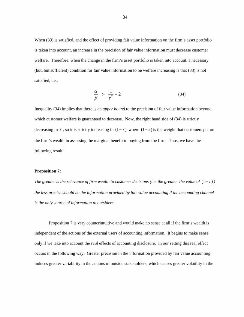
When (33) is satisfied, and the effect of providing fair value information on the firm’s asset portfolio

is taken into account, an increase in the precision of fair value information must decrease customer

welfare. Therefore, when the change in the firm’s asset portfolio is taken into account, a necessary

(but, but sufficient) condition for fair value information to be welfare increasing is that (33) is not

satisfied, i.e.,

21 2a

β τ> − (34)

Inequality (34) implies that there is an upper bound to the precision of fair value information beyond

which customer welfare is guaranteed to decrease. Now, the right hand side of (34) is strictly

decreasing in τ , so it is strictly increasing in (1 )τ− where (1 )τ− is the weight that customers put on

the firm’s wealth in assessing the marginal benefit to buying from the firm. Thus, we have the

following result:

Proposition 7:

The greater is the relevance of firm wealth to customer decisions (i.e. the greater the value of (1 )τ− )

the less precise should be the information provided by fair value accounting if the accounting channel

is the only source of information to outsiders.

Proposition 7 is very counterintuitive and would make no sense at all if the firm’s wealth is

independent of the actions of the external users of accounting information. It begins to make sense

only if we take into account the real effects of accounting disclosure. In our setting this real effect

occurs in the following way. Greater precision in the information provided by fair value accounting

induces greater variability in the actions of outside stakeholders, which causes greater volatility in the

35

firm’s wealth, which induces the firm to become more cautious in its investment strategy which, in

turn, damages the welfare of the firm’s outside stakeholders.

6. Concluding Remarks

The usual debate surrounding MTM accounting is as follows: The FASB and the SEC argue

that marking-to-market a firm’s assets and liabilities improves the accuracy of reported equity.

Professional managers argue that MTM unrealistically increases the volatility of reported income and

reported equity.7 Both arguments are framed in the space of reports. Preferences over reports are not

primitive preferences, so it is difficult to make tradeoffs and welfare comparisons. What we have

done, in this paper, is to explicitly identify an important decision to be made by external agents and we

model how the payoff to such decisions varies with the financial condition of the firm. This allows us

to be precise about how economic agents use MTM information to assess the financial condition of the

firm and adjust their decisions accordingly. In turn, this allows us to quantify the welfare

consequences of providing a more accurate report on the firm’s equity. On the other side of the

argument, we have shown how volatility in reported equity translates into volatility in the firm’s real

wealth/equity, and we have characterized a real decision that corporate managers would change in

anticipation of this increased volatility. All of this allows us to be explicit about tradeoffs and their net

effect on welfare.

Two key ingredients in our model drive the negative welfare results described above. First,

the sequential nature of decisions: Outside stakeholders choose their actions after the accounting

information arrives, but the firm chooses its action before the accounting measurement occurs and in

anticipation of that measurement. Second, both sets of actions affect the object that is of interest to

both parties, viz., the firm’s wealth. We conjecture that both these ingredients are present in most

7 See Beatty, Chamberlain and Magliolo (1996) for an articulation of these arguments.

36

settings where external financial reporting matters in an informational sense. To the extent that this is

true, the approach taken here should be useful for studying many other accounting issues besides fair

value accounting. For, example it would be interesting to study accounting for firms’ hedging

activities from such a perspective. Notably, our approach allows us to endogenously capture both the

costs and benefits of accounting measurement and disclosure, so that there is a meaningful tradeoff

that can be studied.

Such endogenous tradeoffs between costs and benefits have been missing in FASB’s approach

to standard setting and in much of the research in accounting. FASB’s view, as enunciated in the

Conceptual Framework for Financial Reporting (2006) is: “The objective of general purpose external

financial reporting is to provide information that is useful to present and potential investors and

creditors and others in making investment, credit, and similar resource allocation decisions.” There

has been no recognition that firms anticipate and respond to accounting measurements and reports to

external parties, and that these anticipatory actions also affect the welfare of investors and other

stakeholders. The main tradeoff indicated in FASB positions is a tradeoff between “relevance and

reliability” which is difficult to understand in a Bayesian world with rational agents. In such a rational

world, if the only objective of financial reports is to improve external decisions, then any measurement

that has incremental relevant information is valuable and should be disclosed, regardless of how noisy

or unreliable that measurement is. In rational Bayesian updating, noisy measurements are not

misleading; they are simply assigned less weight. In academic research, it is all too common to use

exogenous compliance costs or exogenous proprietary costs to offset the benefits to disclosing more

information.

It may seem that our assumption that customers are risk neutral is a key limitation of our

analysis. What if customers are equally risk averse as the firm’s owners? Unfortunately, an explicit

analysis of how risk aversion among users would change our welfare results cannot be undertaken in

37

the setting that we have studied. This is because, risk averse customers would respond to any

investment in the risky asset by decreasing their demand for the good that they are purchasing from

the firm. Knowing this, the firm would not invest at all in the risky asset, barring some strong and

unrealistic assumptions. Thus there would be no assets that could be marked-to-market. The effect of

risk aversion among users needs to be studied in a different kind of model. However, the assumption

of risk neutrality is not as restrictive as it might seem. As long as the sequential decision making that

we have modeled is preserved, it will always be true that the sensitivity of external decisions to the fair

value signal will cause a sharply increased volatility in the firm’s real equity. This increased volatility

is of concern to the firm’s owners but is of no concern to external decision makers because the

uncertainty in the fair value report is completely resolved by the time external agents need to act. So

the firm is inherently in a more risky position than the external decision makers that rely upon the

accounting information, implying that their preferences over investment in risky assets will generally

not coincide.

38

Appendix

Proof of Proposition 1:

First, we calculate the value of Q from (11). From (14) it follows that:

( 1) 1 1

0 0(1 ) (1 ) [ (1 ) ]t t t t t

t tPτ θ τ δ θ δ

∞ ∞+ + +

= =

− = − + −∑ ∑

0 0 0

[ (1 ) ] (1 ) [ (1 ) ]t t t t t

t t tP Pδθ τ δ τ δ τ δ

∞ ∞ ∞

= = =

= − + − − −∑ ∑ ∑

1 (1 ) 1 (1 )

P Pδθ δτ δ τ τ δ

= + −− − − −

= 1 1

1 (1 ) 1 (1 )Pτδ τδθ

τ τ δ τ δ

+ − − − − −

Inserting this expression into (11) yields the expression described in (16). Now, from (16) it follows that:

1( ) (1 )( ) (1 ) ( ) 1 ( 1)1 (1 ) 1 (1 )i iE Q m z z E P Aτδ τδτη τ τ θ

τ τ δ τ δ = + − − + − + − − − − −

Substituting (A1) into (4) and using ( ) (1 )i iE x Pθ δ δ= + − gives:

1[ (1 )( )] 1 (1 ) [ (1 ) ]

1(1 ) (1 ) 11 (1 ) 1 (1 )

i i

i

q m z z x P

z x P P

ττη τ τ δ δτ

τ τδ τδτ δ δτ τ δ τ δ

− = + − − + + − + − + − − + − + − − − − −

(A2)

39

Collect the terms in (A2) that depend on ix and the terms that depend on .P The term that

depends on ix is:

1(1 ) 1

1 (1 )iz x τ τδτ δτ τ δ

− − + − − =

(1 )1 (1 )

iz xτ δτ δ

−− −

which is convenient to write as:

= 1

1 (1 ) izxτ τδτ τ δ

− − −

(A3)

Also in (A2) the terms that depend on P are:

1 1(1 ) (1 ) 1 11 (1 ) 1 (1 )

zP τ τδ τ τδτ δτ τ δ τ τ δ

− − − − + + − − − − −

= 1 1 1(1 )

1 (1 ) 1 (1 )zP δ τ δτ

τ δ τ τ δ − − − − + − − − −

= 1 1

1 (1 )zPτ δ

τ τ δ − − − −

= 1 1

1 (1 )zPτ τδ

τ τ δ − − − −

(A4)

Inserting (A3) and (A4) into (A2) and simplifying gives:

40

1 (1 )( ) (1 ) 11 (1 ) 1 (1 )i iq m z z x Pτδ τδτη τ τ

τ τ δ τ δ = + − − + − + − − − − −

as claimed in Proposition 1.

Proof of Lemma 1:

Both parts of the Lemma are true if the factor 2 2(1 ) βλ λa β

+ − + is strictly increasing in .β

Using and gives1 (1 )

τδ γλ δτ δ a β γ

≡ ≡− − + +

τγλa β τγ

=+ +

. Therefore the factor:

2 2(1 ) βλ λa β

+ − + =

2 2 2

21( )

τγ τ γ βa β τγ a β τγ a β

+ − + + + + +

2 2 2 2 22

1 [( ) ]( )

βτ γ a β τγ τ γa β τγ a β

= + + + − + + +

= 2 2

2( ) 2

( )τ γ β a β βτγ

a β τγ+ + +

+ +

Therefore,

2 2(1 )sign βλ λβ a β ∂

+ − = ∂ +

2 2 2( ) ( 2 2 ) 2( )( ( ) 2 )sign a β τγ a β τγ a β τγ τ γ β a β βτγ+ + + + − + + + + + =

2 2( )[( )( 2 2 ) 2( ( ) 2 )]sign a β τγ a β τγ a β τγ τ γ β a β βτγ+ + + + + + − + + + =

41

2 2 2 2

( ) [ ( ) 2 ( ) 22 ( ) 2 2 2 ( ) 4 ]

signa β τγ a a β τγ β a β βτγ

τγ a β τ γ τ γ β a β βτγ

+ + + + + + + +

+ + − − + − =

( )[ ( ) 2 ] 0sign a β τγ a a β τγ aτγ+ + + + + >

Q.E.D.

Proof of Proposition 2:

We have previously argued that from the perspective of date 0,

2( ) ( ) var( ) 2 cov( , )var w z var Q z Qθ θ= + + . In Proposition 2 we are holding z fixed and

var( )θ is a prior variance that is unaffected by the precision of accounting disclosure. We have

shown in Lemma 1 that var( )Q is strictly increasing in the precision of public disclosure.

Therefore, it suffices to establish that cov( , )Qθ is also strictly increasing in the precision of

public disclosure. But, from (20), cov( , )Qθ is strictly increasing in β if the factor

(1 ) βλ λa β

+ − + is strictly increasing in .β Inserting

τγλa β τγ

=+ +

gives,

(1 ) βλ λa β

+ − + = 1τγ τγ β

a β τγ a β τγ a β

+ − + + + + +

= β τγ

a β τγ+

+ +

which is strictly increasing in .β

Q.E.D.

Proof of Proposition 5:

42

As derived in (16):

( ) 1 (1 )( ) (1 ) (1 )Q m z z Pτη τ τ λθ λτ

= + − − + − + −

The term (1 )Pλθ λ+ − can be written as:

( ) ( )(1 ) a θ θ µ β θ ελθ λ

a β − + + +

+ − +

= (1 ) ( ) (1 )a βθ λ θ µ λ εa β a β

− − − + − + +

= ( )a βθ θ µ εa β τγ a β τγ

− − + + + + +

where we have used (1 ) a βλa β τγ

+− =

+ + as derived in the proof of Lemma1. Therefore,

1 (1 )( ) (1 ) ( )Q m z z z a βτη τ θ τ θ µ ετ a β τγ a β τγ

= + − − + + − − − + + + + +

Now, we use this last expression for Q to evaluate (26) term by term.

[ ] [ ]

[ ]

21(1 )( ) (1 )(m )

1 (1 )(m ) (1 ) ( )

m z z Q z z

z z z

τη τ θ τη τ θτ

a βτη τ θ τ θ µ ετ a β τγ a β τγ

+ − − + = + − − + +

+ − − + − − − + + + + +

and,

43

[ ]

[ ]

222

2

222

1 (1 )(m )

2 (1 )(m ) (1 ) ( )

1 ( )

Q z z

z z z

z

τη τ θτ

a βτη τ θ τ θ µ ετ a β τγ a β τγ

τ a βθ µ ετ a β τγ a β τγ

= + − − +

+ + − − + − − − + + + + +

− + − − + + + + +

Also, from (15) and (16),

22 2 2 2

2

1( ) (1 ) ( )i iq Q di z x diτγτ θτ a β τγ

− = − − + +

∫ ∫

Therefore, (26) can be expressed as:

[ ] 2 21 1(1 )( ) (2 1) ( )2 2 im z z Q Q q Q diτη τ θ τΩ = + − − + − − − −∫

[ ]22

1 (1 )( )2

m z zτη τ θτ

= + − − + +

[ ]2

1 (1 )( ) (1 ) ( )m z z zτ a βτη τ θ τ θ µ ετ a β τγ a β τγ

− + − − + − − − + + + + +

22 2

2

22 2 2

2

1 (2 1)(1 ) ( )2

1 (1 ) ( )2 i

z

z x di

a βτ τ θ µ ετ a β τγ a β τγ

τγτ θτ a β τγ

− − − − − + + + + +

− − − + +

∫

44

Taking an expectation over the random variables and θ ε and using 2 1[( ) ] var( )E θ µ θa

− = =

and 2 1[( ) ] var( ) ,i iE x xθγ

− = = gives:

[ ]2 2 22 2

1 1 1( | ) (1 )( ) (1 )2 2

E z m z z zτη τ µ ττ τ a

Ω = + − − + + −

2 22

1 (1 ) [( )( )]z Eτ aτ θ θ µτ a β τγ− − − − + +

2 22 2

2

2 1 1 1(1 )2

zτ a βττ a β τγ a a β τγ β

− − − + + + + +

22 2

2 2

1 (1 )2 ( )

z τ γττ a β τγ

− −+ +

Collecting terms and using [( )( )]E θ θ µ− = 2 2 1( ) var( )E θ µ θa

− = = gives,

[ ]22

22 2

2 2 2

1( | ) (1 )( )2

1 1 2(1 )(1 ) (2 1)2 ( ) ( ) ( )

E z m z z

z

τη τ µτ

τ a β τ γτ ττ a a β τγ a β τγ a β τγ

Ω = + − − +

− ++ − − − − − + + + + + +

[ ]22

2 2 22 2

1 (1 )( )2

1 1 1(1 ) (2 2 )( ) (2 1)( )2 ( )

m z z

z

τη τ µτ

τ τ a β τγ τ a β τ γτ a a β τγ

= + − − +

+ − − − + + + − + + + +

45

[ ]22

2 22 2

1 (1 )( )2

1 1 1 (1 )(1 ) ,2 ( ) ( )

m z z

z

τη τ µτ

τγ τττ a a β τγ a β τγ

= + − − +

−+ − − − + + + +

which is the result that we wished to prove.

Q.E.D.

46

References

Allen, Franklin and Elena Carletti, 2008, Mark-to-Market Accounting and Liquidity Pricing, Journal

of Accounting & Economics 45, 358-378

Angeletos, George-Marios and Alessandro Pavan, 2004, Transparency of Information and

Coordination in Economies with Investment Complementarities, American Economic Review, Papers

and Proceedings May, 2004, 91-98.

Barth, Mary, William Beaver and Wayne Landsman, 2001, The Relevance of the Value-Relevance

Literature for Financial Accounting Standard Setting: Another View, Journal of Accounting &

Economics 31,77-104.

Barth, Mary, 2006, Including Estimates of the Future in Today’s Financial Statements Accounting

Horizons 20, 271-85.

Beatty, Anne, Sandra Chamberlain, and Joseph Magliolo, 1996, An Empirical Analysis of the

Economic Implications of Fair Value Accounting for Investment Securities, Journal of Accounting &

Economics 22, 43-77.

Bleck, Alexander and Xuewen Liu, 2007, Market Transparency and the Accounting Regime, Journal

of Accounting Research 45, 229-256.

47

Bond, Philip, Alex Edmans and Itay Goldstein, 2012, The Real Effects of Financial Markets, Annual

Review of Financial Economics 4, 339-360.

Carlsson, H. and Eric Van Damme, 1993, Global Games and Equilibrium Selection, Econometrica

61 (5), 989-1018

Forbes, Steve, End Mark-to-Market, Forbes.com, March 29,2009.

Heinemann, F., Nagel, R. and Ockenfels, P., 2004, Theory of Global Games on Test: Experimental

Analysis of Coordination Games with Public and Private Information. Econometrica 72(5), 1583-

1599.

Kanodia, Chandra, Haresh Sapra and Raghu Venugopalan, 2004, Should Intangibles be Measured:

What are the Economic Tradeoffs, Journal of Accounting Research 42, 89-120.

Kanodia, Chandra, 2006, Accounting Disclosure and Real Effects, Foundations and Trends in

Accounting 1, 167-258.

Kanodia, Chandra and Haresh Sapra, 2016, A Real Effects Perspective to Accounting Measurement

and Disclosure: Implications and Insights for Future Research, Journal of Accounting Research 54,

623-676.

Kydland, Finn. and Edward C. Prescott, 1977, Rules rather than Discretion: The Inconsistency of

Optimal Plans, The Journal of Political Economy 85, No 3, 473-491.

48

Laux, Christian and Christian Leuz, 2009, The Crisis of Fair Value Accounting: Making Sense of the

Recent Debate, Accounting, Organizations and Society 34, 826-834.

Morris, Stephen, and Hyun Shin, 2002, Social Value of Public Information, American Economic

Review, 92(5), 1521-1534.

Plantin, Guillaume, Haresh Sapra and Hyun Shin, 2008, Marking-to-Market: Panacea or Pandora’s

Box? Journal of Accounting Research 46, 435-460.

Wallison, P.J. 2008a, Fair Value Accounting: A Crtique, Financial Services Outlook, American

Enterprise Institute for Public Policy Research, July 2008.

Wallison, P.J. 2008b, Judgment too Important to be Left to the Accountants, Financial Times, May 1,

2008.

Whalen, R.C., 2008, The Subprime Crisis – Causes, Effect and Consequences, Networks Financial

Institute, March 2008.

49