Policy Research Working Paper 9002

Long-Term Effects of PROSPERA on Welfare

Arturo AguilarCristina Barnard

Giacomo De Giorgi

Social Protection and Jobs Global PracticeSeptember 2019

Pub

lic D

iscl

osur

e A

utho

rized

Pub

lic D

iscl

osur

e A

utho

rized

Pub

lic D

iscl

osur

e A

utho

rized

Pub

lic D

iscl

osur

e A

utho

rized

Produced by the Research Support Team

Abstract

The Policy Research Working Paper Series disseminates the findings of work in progress to encourage the exchange of ideas about development issues. An objective of the series is to get the findings out quickly, even if the presentations are less than fully polished. The papers carry the names of the authors and should be cited accordingly. The findings, interpretations, and conclusions expressed in this paper are entirely those of the authors. They do not necessarily represent the views of the International Bank for Reconstruction and Development/World Bank and its affiliated organizations, or those of the Executive Directors of the World Bank or the governments they represent.

Policy Research Working Paper 9002

The long-term effects of Mexico’s conditional cash transfer program, PROSPERA, on poor households are of great interest to policy makers and academics alike. This paper analyzes the long-term effects on the welfare of the original participant households and their offspring, about 20 years after the inception of the program. To complement other studies that look into the effects on schooling and health, the analysis focuses on a utilitarian definition of welfare and employs two empirical strategies. The first uses the 1997–2000 experiment as the cleanest, albeit limited, source of variation. The analysis finds that by 2017–18, the offspring of original beneficiary households are more likely to have formed their own households, to have migrated to differ-ent localities, and to have more durable assets and larger consumption expenditures than their control counterpart.

The second strategy confirms and expands those findings using a difference-in-difference methodology based on the localities’ rollout of the program and the age of the individ-uals, as a proxy of exposure. This second approach covers a much larger and representative sample, while also directly observing self-reported vulnerability in food consumption. The findings confirm the generally positive outlook in terms of durable assets and lower food vulnerability. Perhaps more interestingly and relevant for evaluating the success of the program is that it improved intergenerational mobility. Using the 1997–2000 experiment, the analysis finds that the young adults who benefited from the program improved with respect to their parents in education, assets holding, and income. They appear to be climbing the ladder of assets and income.

This paper is a product of the Social Protection and Jobs Global Practice. It is part of a larger effort by the World Bank to provide open access to its research and make a contribution to development policy discussions around the world. Policy Research Working Papers are also posted on the Web at http://www.worldbank.org/prwp. The authors may be contacted at giacomo.degiorgi@unige.ch and the coordinators of the studies may be contacted at cavilaparra@worldbank.org.

Long-Term Effects of PROSPERA on Welfare ∗

Arturo Aguilar† Cristina Barnard‡ Giacomo De Giorgi§

Keywords: PROSPERA, Social Program, long-term, Welfare.JEL Codes: I38, O12, O15

∗This paper is part of the research project “Studies of PROSPERA’s long-term results” which was funded by theGovernment of Mexico through the National Coordination of PROSPERA (CNP) as part of a technical cooperationagreement with the World Bank. The World Bank team is grateful to the Government of Mexico, including theMinistry of Social Development (now Ministry of Welfare), Ministry of Education, and Ministry of Health, for theclose collaboration in this research project, including the provision of the main datasets. The World Bank teamwould also like to thank the National Council for the Evaluation of Social Development Policy (CONEVAL),the National Institute of Public Health, development partners such as the Inter-American Development Bank,and the national and international researchers that contributed in the Advisory Evaluation Group. This groupwas established to ensure technical quality and methodological rigor of the “Studies of PROSPERA’s long-termresults.” These studies were coordinated by Maria Concepcion Steta, WB Senior Social Protection Specialist;Clemente Avila, WB Social Protection Economist; and Monica Orozco, WB Consultant.†ITAM‡ITAM§GSEM-University of Geneva, MOVE, BGSE, UAB, BREAD, CEPR, IPA

I Introduction

The long-term analysis of Mexico’s conditional cash transfer program (CCT), PROSPERA,constitutes a substantial resource for policy makers, and researchers alike. Mexico’s worldfamous CCT PROSPERA (previously named PROGRESA and Oportunidades), with its focuson human capital investment in terms of health and education, has already inspired severalprograms around the globe and has shaped the way researchers, policy makers, and politiciansinteract on the implementation and evaluation of large policies.1

Moving beyond the short-term analysis will give the opportunity to understand whether theshort-term impacts translate into benefits in the long run, and not only for original beneficiaryhouseholds but also, and most importantly, for their offspring. This analysis is crucial sinceone of the main goals of the program is to break the intergenerational cycle of poverty in whichparents’ conditions worked as a key barrier to their children’s success in life. This would be atremendous accomplishment of any policy and as such deserving of the greatest attention.

In this work, we study the long-term effects of the program by providing answers to thefollowing questions:

1. Did the program improve the long-term welfare of participants?

2. Did the program contributed to break the cycle of poverty of participants and their off-spring (intergenerational mobility)?

Answering these questions is not a simple task. To begin with, the concept of welfare is farfrom being unequivocally determined.2 Atkinson (2011) and Deaton (2018) recently reigniteda decades-long discussion about the proper way to define and measure such an elusive con-cept. Sen (1970, 1973, 1986, 2006) has played a leading role in this debate by challengingan utilitarian approach to welfare and rather promoting a capabilities approach based on theidea that outcomes or decisions (observable to the researcher) portray an incomplete picture ofthe actual well-being of the individual. The ample literature studying PROSPERA’s benefitshas looked into many different dimensions of an individual and household’s life covering wel-

fare from different perspectives. This paper is limited in that sense. We chose to focus on aconsumption-based approach of welfare, which is more in line with the utilitarian view. Theutilitarian perspective of welfare is justified by the fact that from an economics theory perspec-tive, consumption is usually the main input in utility functions.3 While we strive to employa more comprehensive definition of welfare than one based only on consumption and labor

1Appendix A gives a general description of the program.2The references to the conceptual definition of welfare do not intend to be exhaustive. They are just intended

to give a small flavor of these remarkable authors’ extensive work on the topic.3For example, in the motivation for the Nobel prize awarded to Angus Deaton in 2015: ...The consumption of

goods and services is a fundamental determinant of human welfare.... https://www.nobelprize.org/nobel prizes/economic-sciences/laureates/2015/advanced-economicsciences2015.pdf.

2

supply, our analysis is complementary to other papers that are being produced as part of thisset of studies, which look into education, health and occupational mobility. Also, at the timeof writing, we are constrained by the data availability, while future work could include severalother indicators as data become more available.

The consumption-based approach to welfare used in this paper will focus mainly on owner-ship of durable goods, while also proposing a measure of (imputed) non-durable consumption(food, personal products, and clothing). This is justified by the fact that consumption reflectsa household’s permanent income level and its resilience to shocks (Deaton and Zaidi 2002).It also reflects better than income the household’s life conditions. In fact, this explains whyPROSPERA’s targeting used a proxy-means test index based on household durables and house-hold members characteristics to identify vulnerable households to be served (Skoufias et al.2001). Secondly, we will look into measures of success by looking into labor market outcomesof those individuals that as children were encouraged by the program to stay enrolled in school.Finally, to look into the intergenerational transmission of poverty we look into measures of mo-bility in the percentile rankings, as in Chetty et al. (2014) of selected outcomes. Our definitionof mobility is now fairly standard in the literature and focuses on the relative position in theoutcome distribution of individuals with respect to their parents. In practice this means thatwe order our data in ascending order on the magnitudes of the outcome of interest for parentsand offspring separately, this ordering would give us a relative position in the relevant distribu-tion. We then compare the relative position of the parents to that of the offspring. If they haveexactly the same position there is no mobility across generations; if those at the bottom seetheir offspring climb up the ladder, we have upward mobility; and the largest mobility wouldbe found if the position of the parents were to be unrelated to that of the offspring.

In the best case scenario, we would find that by (i) allowing families to insure against tem-porary shocks, (ii) lifting incomes to higher and more stable levels, and (iii) through the in-vestment in both physical and human capital (education, and health) the program can generatea virtuous cycle. This could be reflected in the investment and improvements of outcomes forbeneficiaries and their offspring, potentially lifting future generations out of poverty. We de-fer to future work the extensions to other aspects and approaches to welfare analysis, whilewe already directly speak to a multifaceted strategy that includes multiple indicators (see forexample Ravallion (2011)), and measures of social deprivation, as the ones suggested by theNational Council for the Evaluation of Social Development Policy (CONEVAL).4

The second challenge we face is methodological. We should note here that a large part ofthe analysis focuses on the long-term effects of the original experimental design, which is thecleanest identification strategy and source of variation in this context, but comes at a high cost.Essentially, the experimental variation gives an early versus late treatment difference. This

4See https://goo.gl/aQ8MPt

3

early-late dichotomy is just a little more than a year of extra transfers for the treated group, orabout 9% additional resources available during the first period of the experiment as the controlgroup began receiving transfers just after the initial experiment. This design therefore is morean intensive margin of treatment rather than an extensive one.5 In a way, the estimated effectscould be understood as lower bounds for the true effects out of an extensive treatment andtherefore any positive effect should be taken as a success of the program given the limitedvariation in the available data. Importantly, we also implement an alternative research designwhich allows us to get closer to the treatment versus pure control exercise; in that approach weuse the program sequential roll-out and individual ages to identify the effect of several years oftreatment versus never directly treated status as those children older than 16 at the time of theintroduction of the policy would not be directly exposed to it (or in any case to a much lesserextent as they would be unlikely to satisfy the age requirement for the conditional components).

The main effects of PROSPERA can be summarized as follows: (i) newly formed house-holds, those of the offspring of the initial and original beneficiary households, see a substantialincrease in their durable purchases in particular for entertainment and kitchen goods as well asfor (imputed) non-durable consumption expenditures; (ii) original households do not appear tohave a large increase in durables; and (iii) new households tend to locate in different localitiesthan those where they lived in 1997 (usually where they were born). These results are consis-tent with the fact that the offspring of the original households are the direct recipients of theadditional human capital both in health and education due to the program, therefore they appearto be on a different long-term development path than their control counterpart. In particular,we see that the largest effects are concentrated among those with the largest initial effects onhuman capital accumulation in the sample: those who were at the verge of dropping out of sec-ondary school in 1997/98, i.e. those who were aged 11-16. We need to remind the reader thatthe experiment used for this part of the analysis lasted between 1998 and 1999. Hence, whileit is possible that there could be large improvements in the very young children (e.g. aged 0-5in our analysis), this would become evident in terms of assets by the time their human capitalaccumulation ends, which is not possible to observe in our exercise. In fact, when we lookat a different data source and provide a complementary research design, in Section V.B, wefind that the effects of PROSPERA are generally largest for beneficiaries affected since theirdevelopmental stages.

In terms of intergenerational and lifecycle mobility, we find that young adults who formedtheir own households fare substantially better than their parents in terms of schooling, assets,

5The intensive margin refers to a comparison of receiving more with respect to receiving less. In contrast,the extensive margin refers to a comparison of receiving an intervention with respect to not receiving it. In ourcontext, the group that was initially defined as the control, began to receive the benefits of the program in 1999.Hence, the treatment versus control comparison should be interpreted as one in which the treatment received moreresources (9% more transfers in total) since their enrollment to the program was earlier (a little more than oneyear). This explains why we assume our comparison to be in the intensive margin.

4

and income when compared to their control counterparts. These latter results are very encour-aging, as exactly that was the aim of the policy. A program like PROSPERA should ultimatelyallow the next generation to thrive and climb the ladder of society, thus breaking the cycle ofpoverty. Finally, to estimate the benefits of PROSPERA throughout its existence, we providea back-of-the-envelope exercise that draws upon Gertler et al. (2012). We compute the effectson non-durable consumption expenditure for the 1997-1999 treated households compared toa control group that does not receive any transfer. Such exercise estimates an effect of about25%, per adult equivalent, over the baseline consumption in 1997 (at 2017 prices).

The remainder of the paper includes a selected review of the literature (Section II); a descrip-tion of the potential mechanisms through which the program can have long-term consequenceson the lives of the original households as well as their offspring (Section III); a thorough de-scription of the data employed (Section IV), and the empirical strategies adopted (Section V).We will then move on to the results in Section VI, and finally conclude in Section VII.

II Literature Review

In order to locate the contribution of our work in the now vast literature on PROSPERA we willmention below the more relevant papers on which we build upon. It is important to mentionthat there are several papers analyzing the short and medium term effects of the program ondifferent outcomes of interest for our work. It would be beyond the scope of the current paper tohave a fully exhaustive list of all the publications that over the past two decades have analyzedthe program, we will just focus on a selection of studies closely related to our own. Despitethe large literature, very few papers have looked into the specific aspects of long-term successthat we focus on, in this sense we see our work as complementary to the amount of knowledgeaccumulated over the years for two main aspects: i. our main focus is on welfare through astandard definition of purchasing/consumption behavior; ii. needless to say we are interestedin the long-term implications of the policy not solely in terms of looking at the 20 years ofoutcomes, but, perhaps more important, is our interest on the next generation or the offspringof original households involved in the program since its inception.

For example, there are a number of studies on the impact of the policy on the consumptionprofiles of beneficiaries (Hoddinott and Skoufias 2004) and non-beneficiaries (Angelucci andDe Giorgi 2009 and Angelucci et al. 2017). These studies find robust evidence of increase inconsumption of non-durables (food mostly) and to a lesser extent of durables for both recipienthouseholds and other family members residing in the same locality as the direct transfer recip-ients. Importantly, Angelucci et al. 2017 look at whether such positive impacts persist in themedium term, defined there as six years since the initial transfers.

A more limited literature on longer term impacts of PROSPERA is available, and, in general,

5

of long-term effects studies of CCT programs. Millan et al. (2018) give a recent summary ofpapers investigating long-term effects of these policies. Relevant examples include: analysis onlong-term effects on human capital (Barham et al. (2017) study a CCT in Nicaragua); similarly,Baez and Camacho (2011) study the long-term effects of the Colombian CCT (Familias en Ac-

cion) on human capital; similar analyses are presented in Barrera-Osorio et al. (2017) and Aizeret al. (2016) on children’s longevity, educational attainment, nutritional status, and income inadulthood in the U.S. There is also a literature looking into different aspects of the transfers:conditional versus unconditional (Baird et al., 2011; Bursztyn and Coffman, 2012), targetedversus universal (Niehaus et al., 2013), as well as other aspects of the transfers (Haushoferand Shapiro, 2016). However, determining aspects of the transfers is beyond the focus of ouranalysis.

For the case of Progresa/Oportunidades/PROSPERA, Behrman et al. (2011), Gertler et al.(2012) and Angelucci et al. (2017) look at the medium-term effects on consumption, humancapital, and investment behavior. Later, Kugler and Rojas (2018) investigate the long-term ef-fects on human capital and labor market outcomes for the original experimental population.Also recently Parker and Vogl (2018) focus on the children of original beneficiary householdsand find positive effects on human capital, assets, housing and labor market outcomes. Fi-nally, Adhvaryu et al. (2018) study how PROSPERA protected children from early life shocks,helping them escape from potentially long-term adverse shocks.

III Potential Mechanisms

There are potentially many channels through which PROSPERA might change the lives ofbeneficiaries, and non-beneficiaries alike. This section is meant to present a stylized theory ofchange rather than a detailed account of the possible mechanisms through which PROSPERAmight have long-term effects. There are potentially many such channels, which depend onwhether one looks at the original beneficiary households or their offspring, so that a detailedaccount would be beyond the scope of this paper. However, we will build upon other authors’work to motivate our own approach and analyze our results.

As is well known, the program was designed to tackle multiple aspects of poverty and howto escape it. In particular, the program targeted education, health, and nutrition through trans-fers and conditionalities. It is therefore immediate to think that for the children of the originalhouseholds a direct virtuous channel going through the accumulation of human capital shouldexist. A larger human capital would then improve the livelihoods for the treated in a stable man-ner. The children of the original beneficiaries are by 2017/8 adults themselves, and given thehigher schooling and better health they can be more productive and earn higher incomes. Suchhigher permanent incomes, and human capital, would then translate into better living standards.We will confirm here that indeed PROSPERA increased the human capital, in terms of school-

6

ing, and health of the children of the original households. There are, however, other importantpotential channels from i. asset accumulation, to ii. occupation, and iii. entrepreneurship.There is by now plenty of evidence on the positive effects on educational and health outcomes(Todd and Wolpin 2006; Angelucci et al. 2010; Bobonis 2009; Lalive and Cattaneo 2009; At-tanasio et al. 2012; Parker and Vogl 2018) for both beneficiaries and non-beneficiaries. Also,evidence has been shown about occupational choices and investment behavior (Bianchi andBobba 2010; Gertler et al. 2012; Angelucci et al. 2017). In addition, the program has proveneffects on occupational mobility (Yaschine 2012), and female empowerment and householddecision processes (Attanasio and Lechene 2002, Attanasio and Lechene 2014, Bobonis et al.2015). All this literature asserts that the original households’ members are more educated, andappear to have accumulated more productive assets, as well as initiated productive businessactivities. The general consensus emerging from the literature is that PROSPERA has achievedsubstantial improvements in the short to medium term as a result of higher human capital, morestable income flows, and profitable investment into assets and occupations.

We build on all this existing evidence to make the case for the long-term and intergenera-tional effects on our main measures of well being. In general, savings and therefore investmentcan rise due to a larger disposable income and reduced general uncertainty for beneficiaryhouseholds. Higher incomes can afford previously unattainable investments, while lower un-certainty in terms of future income streams lowers the need for precautionary or unproductivesavings, while allowing households to take more risk into business ventures (Banerjee andDuflo, 2011). Similarly, better educated individuals might be making better long-term con-sumption decisions. Previously severely credit constrained beneficiary households can nowstart saving and investing for the long-term and their offspring.

We acknowledge that all these channels, or more, could be in operation at once. Even thoughwe will discuss some channels when relevant, attempting to decompose the overall effects oneach channel is not the purpose of the present study. Rather, we focus on estimating the overallpolicy effect of the program on different measures that reflect higher wellbeing. Doing so isempirically challenging given that original experiment variation provides only a small windowof differential exposure. Two aspects of such differential exposure will be exploited in ouranalysis: first, the fact that households in experimental localities receive a larger aggregateamount and time exposure to resources. Second, in parts of the analysis we will pair this withcohort variation, which gives differential exposure at critical stages. Two meaningful examplesare: educational stages in which high levels of dropouts are frequent (especially among poorrecipients) and critical early developmental stages. For both cases, the literature on the programhas already provided favorable evidence.

7

IV Data

We employ two data sources for the analysis presented here: (1) the PROSPERA panel datagathered, since 1997 all the way to 2017-2018 (on a subset of localities and individuals), for theevaluation of the initial experiment and (ii) the 2015 intercensus data collected by the NationalInstitute of Statistics and Geography (INEGI).

IV.A PROSPERA ENCEL panel

As it is widely known, in 1997 a sample of 24,077 households in 506 rural localities wasselected to implement a randomized controlled trial (RCT) in order to give robust evidenceabout the effects of PROSPERA (known as Progresa at that time).6 This set of localities,chosen according to the administration of the program guidelines, where then allocated to atreatment (320 localities) and a control group (186 localities) where the eligible householdsin treatment group received PROSPERA’s support, transfers were distributed to those eligiblehouseholds who complied with the stated rules of the program, starting in the fall of 1998while the control localities started to receive the same treatment at the very end of 1999. Suchsample was followed up with a survey instrument called ENCEL in 1998, 1999, 2000, 2003and 2007 to give evidence of short and medium-run impacts of the program. In an effort toprovide relevant data to evaluate the effects of PROSPERA in the long-run, the World Bank,PROSPERA and the National Institute of Public Health (INSP) partnered to gather informationin 2017-2018 on a subset of that sample of participants.

ENCEL 2017-2018 sampling framework. Given the budgetary restrictions and the com-plexity of tracking back the original participants, which was the strategy of the previous roundsof the panel, a sub-sample of 334 localities of the 506 original localities was selected.7 AsPanel A in Table 1 shows, this first filter meant that richer eligible households in less marginal-ized localities would become the sample target. Each of the selected localities was visited andthe surveyors looked for the 18,564 households included in the 1997 sample that inhabited thatlocality. The targeting strategy employed at the beginning of the program to select beneficiariesdefined 12,519 of these households as eligible. We will focus our analysis in this set of house-holds, since they provide the variation that would be relevant for the analysis.8 Priority wasgiven to households that had young members at the start of the data collection (1997-2000).In total, 7,824 eligible households were located in the 2017-18 data collection. Hereon, we

6At the beginning of the program, priority was given to rural localities. In Mexico, rural localities are definedas those with fewer than 2,500 inhabitants.

7Localities that were more accessible and as a result richer within the 506 original full sample were selectedfor the ENCEL 2017-18. A set of localities that were added in the 2003 round are not included in the samplingframework for the 2017-18 round.

8Non-eligible households could have enrolled later to the program. However, comparing non-eligible house-holds from treatment and control communities would involve selecting households that initially did not receivethe program and were not affected by the random allocation of treatment.

8

will refer to them as the original households, since their sampling took place back in 1997.Panel B in Table 1, shows the attrition resulting from the inability to locate some of the originalhouseholds in the 334 selected localities. Larger households with more assets are more likelyto be surveyed in 2017. Importantly, and central for the internal validity of the estimated ef-fects, we show that the overall attrition described appears orthogonal to treatment (see Table

2). This latter result is reassuring in terms of causal identification of the treatments effects,however we should mention that those effects might not be applicable to the entire populationof interest. Despite that concern we conjecture that the sampling framework adopted is likelyto produce underestimates or conservative estimates of the effects as the sample, includes betteroff households to start with, and it is plausible that the program effects would be smaller forthose households.

Next, using a list of all the individuals in the 1997 original households, surveyors asked forsocio-demographic information about each of them, as well as for the new members living inthe household (these would be offspring or other individuals entering the household after the1997 survey round). Among the original set of individuals, a separate survey was designed formembers that were in critical age groups at the time in which the program started. Three agegroups of interest were then defined: (i) newborns in 1997-2000, since they were in a criticalstage of development when the RCT took place; (ii) children 6 to 8 years old in 1997-2000,since they were about to enroll in school grades where the program’s conditionalities are mostrelevant; and (iii) children in sixth grade in 1997-2000, since the program’s positive effects interms of later school enrollment appear to be concentrated in this critical grade.

Importantly, these individuals could be still living in the original households, but they couldhave also moved out to form a new household (or joined an existing one). Contact informationwas recorded to track these individuals. This search process had a geographic limitation: in-terviews with individuals that moved out of the original household were only attempted if theysettled in the same locality as the original household, within a short range of the original house-hold’s locality9 or in the three main metropolitan areas in Mexico (Mexico City, Monterrey andGuadalajara). As mentioned above, the households where these individuals were located couldbe either newly formed households (e.g. the individuals married or just decided to move out bythemselves) or could be households that already existed and the individual decided to move in(e.g. moving with relatives). For the purpose of our analysis we define all these households asnew households in the sense that they did not exist in the 1997 sample.

Surveyors were able to locate and interview 4,987 individuals in the relevant group ages:2,105 of them were still in their original households and the remaining 2,882 were in newhouseholds. Of the individuals living in a new household, 4,207 interviews were not success-fully completed, either because they moved to a household not accessible given the survey

9Given budgetary restrictions, households were searched in localities located within a 30 minute driving dis-tance at most.

9

Tabl

e1:

Attr

ition

tabl

e.Pa

nelA

:Geo

grap

hica

lsel

ectiv

eat

triti

onPa

nelB

:Res

pons

ese

lect

ive

attr

ition

Mea

nM

ean

1997

Var

iabl

esL

ocal

ities

out

Loc

aliti

esin

Diff

p-va

lues

Non

-res

pond

ents

Sam

ple

Diff

p-va

lues

Hou

seho

ldhe

adch

arac

teri

stic

sFe

mal

e*0.

0898

0.08

28-0

.006

90.

3419

0.10

400.

0579

-0.0

462

0.00

00A

ge43

.178

742

.146

8-1

.031

90.

0447

43.6

988

40.3

251

-3.3

737

0.00

00Y

ears

ofsc

hool

ing

2.61

002.

7620

0.15

200.

2534

2.60

302.

9477

0.34

470.

0000

Inco

me

and

prod

uctiv

eac

tiviti

esH

Apr

oduc

tive

land

1.78

811.

6975

-0.0

906

0.57

111.

6422

1.76

280.

1206

0.18

72lo

g(H

Hm

onth

lyin

com

ePC

)5.

0339

4.95

82-0

.075

80.

0706

5.06

244.

8391

-0.2

233

0.00

00

HH

.Cha

ract

eris

ticsa

ndas

sets

Dir

tfloo

r*0.

7661

0.73

65-0

.029

60.

2382

0.76

190.

7066

-0.0

553

0.00

00E

lect

rici

ty*

0.48

550.

6107

0.12

520.

0066

0.56

800.

6612

0.09

320.

0000

Ref

rige

rato

r*0.

0324

0.04

170.

0093

0.34

160.

0385

0.04

560.

0071

0.09

04Te

levi

sion

*0.

2762

0.30

480.

0285

0.29

210.

2661

0.35

040.

0843

0.00

00D

raft

anim

als

owne

rshi

p*0.

3488

0.33

08-0

.018

00.

4476

0.29

700.

3707

0.07

380.

0000

Hou

seho

ldde

mog

raph

ics

Hou

seho

ldsi

ze5.

6965

5.96

630.

2699

0.00

065.

2133

6.85

561.

6423

0.00

00N

umch

ildre

n0-

71.

5602

1.67

900.

1188

0.00

901.

3172

2.10

570.

7885

0.00

00N

umch

ildre

n8-

171.

6560

1.77

730.

1213

0.00

411.

4641

2.14

710.

6830

0.00

00N

umad

ults

70+

0.13

140.

1006

-0.0

308

0.00

200.

1264

0.07

01-0

.056

30.

0000

Loc

aliti

esch

arac

teri

stic

sL

ocal

itym

argi

naliz

atio

nin

dex

1995

0.72

290.

6272

-0.0

957

0.29

850.

6643

0.58

33-0

.080

90.

0309

Num

.obs

erva

tions

2,71

89,

801

5,30

74,

494

Join

ttes

t:F-

stat

=2.

02;p

-val

ue=

0.12

8Jo

intt

est:

F-st

at=

80.0

4p-

valu

e<

0.00

00*

Dum

my

vari

able

Thi

sta

ble

show

sth

ese

lect

ive

attr

ition

base

don

the

geog

raph

ical

rest

rict

ion

esta

blis

hed

tose

lect

the

sam

ple

and

the

capa

bilit

yto

find

the

orig

inal

hous

ehol

dsfr

omth

e19

97E

NC

ASE

Hsa

mpl

e.B

alan

ceof

vari

able

ssh

own

are

calc

ulat

edw

ithth

e19

97E

NC

ASE

Hda

ta.

Stan

dard

erro

rscl

uste

red

atth

elo

calit

yle

vel.

Ast

eris

ksin

dica

tesi

gnifi

canc

eat

the

***1

%,*

*5%

,and

*10%

leve

l.

10

Table 2: Balance table.Mean

1997 Variables Control Treatment Diff p-value

Household head characteristicsFemale* 0.0571 0.0583 0.0012 0.8868Age 40.5610 40.1865 -0.3745 0.4146Years of schooling 2.8088 3.0293 0.2205 0.1457

Income and productive activitiesNum. productive ha of land 1.7492 1.7708 0.0215 0.9048log (HH monthly income PC) 4.8815 4.8130 -0.0685 0.1003

HH. Characteristics and assetsDirt floor* 0.7271 0.6945 -0.0326 0.2831Electricity* 0.6679 0.6572 -0.0106 0.8239Refrigerator* 0.0463 0.0452 -0.0011 0.9262Television* 0.3751 0.3359 -0.0392 0.2528Draft animals* 0.3518 0.3818 0.0301 0.3222

Household demographicsHousehold size 6.8539 6.8566 0.0027 0.9770Num children 0-7 2.1263 2.0936 -0.0327 0.5062Num children 8-17 2.1323 2.1558 0.0235 0.6716Num adults > 70 0.0692 0.0706 0.0015 0.8689

Localities characteristicsMarginalization index 1995 0.6748 0.5296 -0.1452 0.1352Num. observations 1,663 2,831

* Dummy variable

This table tests balance in observable characteristics between the PROSPERA RCT original treat-ment and control with our sample. Observations are restricted to those households that were found inENCEL 2017-18 and employed in our main estimations. Balance of variables shown are calculatedwith the 1997 ENCASEH data. Standard errors clustered at the locality level. Asterisks indicatesignificance at the ***1%, **5%, and *10% level.

11

geographical coverage, individuals were not found in the address given to surveyors or they didnot respond. In addition, a sub-sample of 1,994 individuals outside the relevant age groups wasmistakenly surveyed.10 In our analysis we use all the individuals sampled.

Table 3 gives further detail about the different possibilities of sample attrition. In this tablewe use a logit model to relate household baseline characteristics with the probability of attrition.Even columns add the interaction of the baseline characteristics with the treatment dummy tofurther explore the possibility of selective attrition. In columns (1) to (4) we present evidenceabout the attrition of the original households, which are the foundation of the sampling design.Columns (1) and (2) give evidence of the locality selection (similarly as in Table 1 Panel A)while columns (3) and (4) give evidence of the possibility to find respondents in the selected334 localities. As these columns show, older head members of smaller households are morelikely to be missing. This is consistent with the evidence presented in Table 1, where wefound no evidence of selective attrition. Finally, columns (5) and (6) include newly formedhousehold attrition. Given that these households did not exist in 1997, its attrition is based onthe possibility to find members in the relevant ages that moved out of the original household. Inthis sense, the attrition results from the 4,207 members who were searched for and not found.Section VI.A.3 does a robustness exercise where inverse probability weights are employed toadjust for attrition.

Available information. Both for original and new households, dwelling’s characteristics andinformation on durable assets were gathered at the household level, we use such informationto explore PROSPERA’s long-term impacts on welfare. Individuals in the critical age groupsdescribed were asked several additional questions on income and work-related topics. An im-portant limitation of the ENCEL 2017 data is that non-durable consumption (crucially includingfood consumption) is not available. This somewhat constrains our welfare analysis, especiallyfor a poor population context, where food expenditure represents a high proportion of total ex-penditures. However, as an additional exercise, we propose an imputed measure on non-durableconsumption expenditure, which includes food, personal products, and clothing, adapting themethodology of Blundell et al. (2005) and Attanasio and Pistaferri (2016) to the available dataand context (see Appendix Section C). It is important to remind the reader that while durableconsumption items are typically bigger ticket items, their purchase is infrequent, and for poorhouseholds the total expenditure on durables is typically about 20% of total expenditure, so thatproviding evidence on non-durable expenditure seems rather important.

Table 4 gives descriptive statistics for the original and new households employed in ouranalysis using 1997 and 2017 data. For new households, the 1997 information corresponds tothat of their respective household of origin. The comparison between 1997 and 2017 shows an

10These individuals added by mistake are not a random sub-sample of all the individuals out of the group ofinterest, but correspond to those for whom age was not available in 1997-2000 and were mistaken for newborns.

12

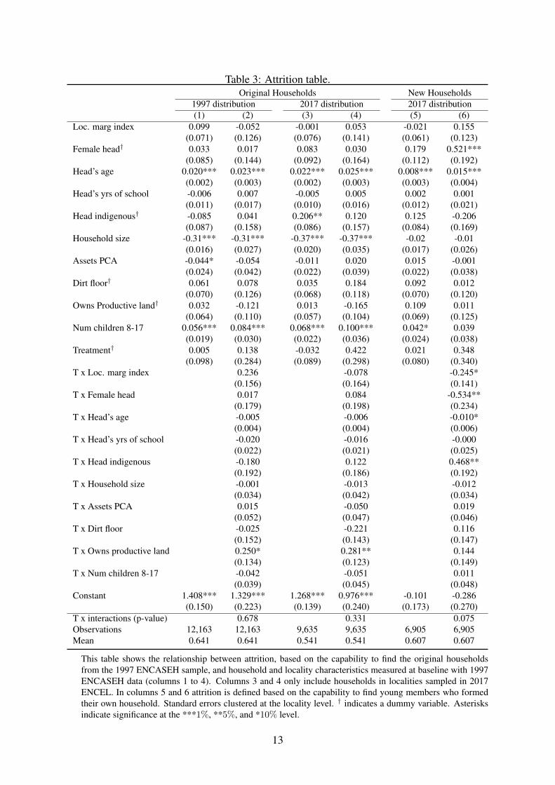
Table 3: Attrition table.Original Households New Households

1997 distribution 2017 distribution 2017 distribution(1) (2) (3) (4) (5) (6)

Loc. marg index 0.099 -0.052 -0.001 0.053 -0.021 0.155(0.071) (0.126) (0.076) (0.141) (0.061) (0.123)

Female head† 0.033 0.017 0.083 0.030 0.179 0.521***(0.085) (0.144) (0.092) (0.164) (0.112) (0.192)

Head’s age 0.020*** 0.023*** 0.022*** 0.025*** 0.008*** 0.015***(0.002) (0.003) (0.002) (0.003) (0.003) (0.004)

Head’s yrs of school -0.006 0.007 -0.005 0.005 0.002 0.001(0.011) (0.017) (0.010) (0.016) (0.012) (0.021)

Head indigenous† -0.085 0.041 0.206** 0.120 0.125 -0.206(0.087) (0.158) (0.086) (0.157) (0.084) (0.169)

Household size -0.31*** -0.31*** -0.37*** -0.37*** -0.02 -0.01(0.016) (0.027) (0.020) (0.035) (0.017) (0.026)

Assets PCA -0.044* -0.054 -0.011 0.020 0.015 -0.001(0.024) (0.042) (0.022) (0.039) (0.022) (0.038)

Dirt floor† 0.061 0.078 0.035 0.184 0.092 0.012(0.070) (0.126) (0.068) (0.118) (0.070) (0.120)

Owns Productive land† 0.032 -0.121 0.013 -0.165 0.109 0.011(0.064) (0.110) (0.057) (0.104) (0.069) (0.125)

Num children 8-17 0.056*** 0.084*** 0.068*** 0.100*** 0.042* 0.039(0.019) (0.030) (0.022) (0.036) (0.024) (0.038)

Treatment† 0.005 0.138 -0.032 0.422 0.021 0.348(0.098) (0.284) (0.089) (0.298) (0.080) (0.340)

T x Loc. marg index 0.236 -0.078 -0.245*(0.156) (0.164) (0.141)

T x Female head 0.017 0.084 -0.534**(0.179) (0.198) (0.234)

T x Head’s age -0.005 -0.006 -0.010*(0.004) (0.004) (0.006)

T x Head’s yrs of school -0.020 -0.016 -0.000(0.022) (0.021) (0.025)

T x Head indigenous -0.180 0.122 0.468**(0.192) (0.186) (0.192)

T x Household size -0.001 -0.013 -0.012(0.034) (0.042) (0.034)

T x Assets PCA 0.015 -0.050 0.019(0.052) (0.047) (0.046)

T x Dirt floor -0.025 -0.221 0.116(0.152) (0.143) (0.147)

T x Owns productive land 0.250* 0.281** 0.144(0.134) (0.123) (0.149)

T x Num children 8-17 -0.042 -0.051 0.011(0.039) (0.045) (0.048)

Constant 1.408*** 1.329*** 1.268*** 0.976*** -0.101 -0.286(0.150) (0.223) (0.139) (0.240) (0.173) (0.270)

T x interactions (p-value) 0.678 0.331 0.075Observations 12,163 12,163 9,635 9,635 6,905 6,905Mean 0.641 0.641 0.541 0.541 0.607 0.607

This table shows the relationship between attrition, based on the capability to find the original householdsfrom the 1997 ENCASEH sample, and household and locality characteristics measured at baseline with 1997ENCASEH data (columns 1 to 4). Columns 3 and 4 only include households in localities sampled in 2017ENCEL. In columns 5 and 6 attrition is defined based on the capability to find young members who formedtheir own household. Standard errors clustered at the locality level. † indicates a dummy variable. Asterisksindicate significance at the ***1%, **5%, and *10% level.

13

increase in levels of education, greater income levels, more asset accumulation; original house-holds aged and became more adult-based; new households are younger in general (both interms of head age and members composition). Interestingly the proportion of female heads im-portantly increases.11 Several reasons explain this change: females are the transfer recipients,this means that single-parent households would tend to be female, but also that when askedfor the head 20-years after the program the likelihood of appointing the female (at least to thesurveyor) is greater; overtime, female widows are more likely than male widowers; and finallyupon households split it is more likely for the female to keep the children and the resources ofthe program.

Table 4: Descriptive Statistics.Original HH New HH

1997 2017 1997 2017Household head characteristics

Female* 0.06 0.26 0.06 0.13Age 40.33 56.82 41.00 31.25Years of schooling 2.95 3.33 2.88 7.76Incomelog(HH monthly income PC) 4.84 7.35 4.85 7.14HH characteristics and assets

Dirt floor* 0.71 0.14 0.69 0.13Electricity* 0.66 0.98 0.66 0.97Refrigerator* 0.05 0.66 0.04 0.56Television* 0.35 0.83 0.36 0.82HH demographics

Household size 6.86 2.47 7.34 3.84Num children 0-7 yrs 2.11 0 2.26 1.08Num children 8-17 yrs 2.15 0 2.38 0.66Num children 18-34 yrs 1.35 0.73 1.46 1.62Num children 35-54 yrs 0.967 0.86 1.01 0.39Num children 55-69 yrs 0.194 0.67 0.20 0.04Num adults 70+ yrs 0.070 0.17 0.07 0.02Localities characteristics

Marginality index (1995) 0.58 0.58Observations 4,494 2,265

* Dummy variablesThis table shows descriptive statistics of household and individual level variables that we will use to build ourmain dependent variables, as well as controls that we will use in our main specifications. Data comes from:(i) 1997 ENCASEH, which corresponds to the baseline data for the Progresa experiment and (ii) 2017-18ENCEL, which is the latest round of the experiment’s panel.

11It is important to indicate that these proportions of female headship are among eligible households.

14

IV.B INEGI’s 2015 Intercensus

A second part of the analysis that will be detailed in the next section uses the 2015 intercensalsurvey, which is collected by INEGI.12 This survey is gathered at the midpoint between cen-suses and contains information on individual’s income, education, dwelling’s characteristics,durable asset ownership, and consumption vulnerability measures (among other things). Thesurvey includes information from individuals in more than 6 million households from all Mexi-can municipalities. The access to this data with restricted geographical identifiers was obtainedthrough INEGI’s microdata lab.13 Our analysis focuses on individuals aged 0 to 21 in 1997-2000 as those individuals had the highest potential exposure to PROSPERA. In total, we use1,875,039 individuals in all the localities (urban and rural) from 24 Mexican states in our anal-ysis.14 Importantly, the use of this ulterior data source allows to look directly into measuresof food consumption insecurity and resilience, while also allowing for a sharper definition oftreatment status as we will explain later. At the same time with this much larger sample, we arealso able to validate the results obtained from the previous data sources, in a fully representativesample of the Mexican population.15

V Empirical Strategy

V.A Analysis Using the PROSPERA ENCEL Panel

Long-Term Effects. For identification of the long-term effects of PROSPERA, we first relyon the 1997-2000 RCT experiment, which gives the cleanest source of variation available.However, since the control localities became treated about two years after the start of Progresa(i.e. by the end of 1999), this strategy should be interpreted as an early versus late treatment oras a treatment intensity deriving from the extra months of transfers the original treated received.Table 5 convincingly shows that original households in early treatment localities receive 8.8%

larger transfers, during 6.6 additional two-month installments. However, these additional re-sources are not evenly distributed during the 20 year period between the start of the programand 2017, rather they are concentrated in 1998-99.

12Available at https://goo.gl/5EMD7e13For confidentiality reasons, INEGI does not disclose the geographical identifiers for localities with fewer than

15,000 inhabitants. The researchers filled up a request to gain access to this information which is critical for theidentification used.

14The selection of Mexican states for the analysis was based on the fact that a discontinuous jump was visu-ally identified in the selection of localities. The states left out include Aguascalientes, Baja California, Colima,Chihuahua, Mexico City, Morelos, Nayarit, and Yucatan.

15Even though the exclusion of Mexico City might strike as harmful for the representativeness of the sample,it is important to remember that the urban extension of the program did not occur until 2004. At that time littlevariation of inclusion was left geographically, which is our main identification strategy here.

15

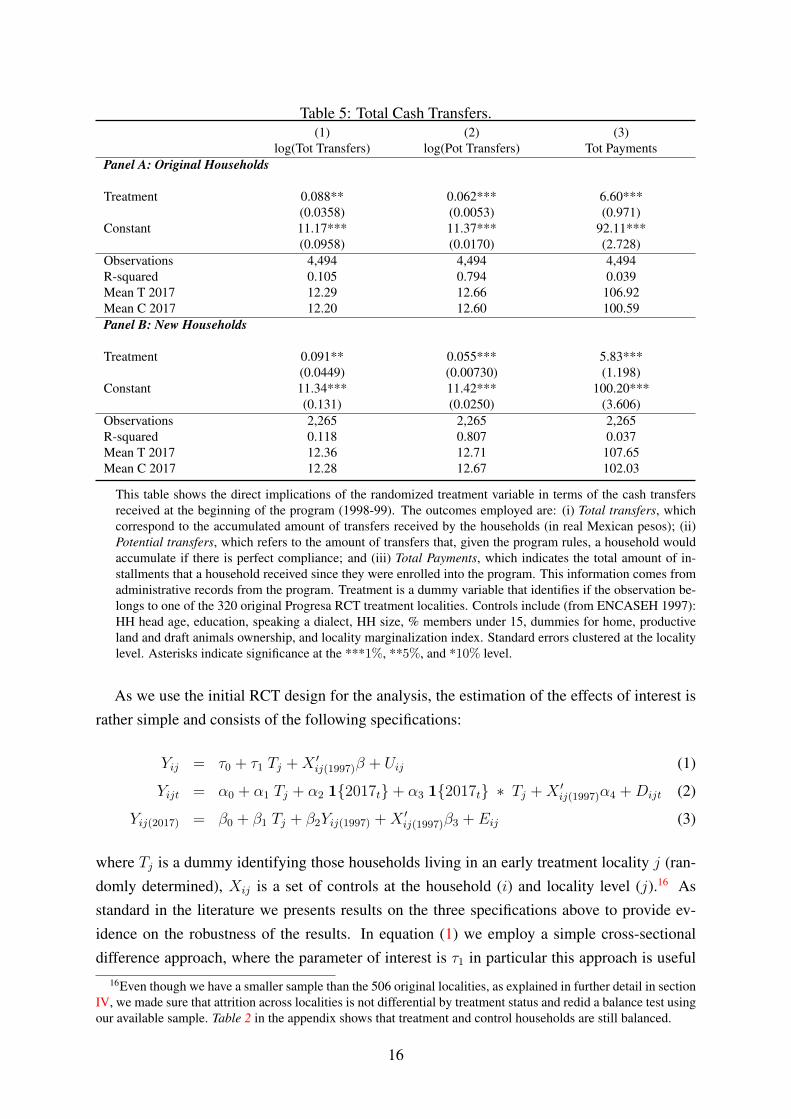
Table 5: Total Cash Transfers.(1) (2) (3)

log(Tot Transfers) log(Pot Transfers) Tot PaymentsPanel A: Original Households

Treatment 0.088** 0.062*** 6.60***(0.0358) (0.0053) (0.971)

Constant 11.17*** 11.37*** 92.11***(0.0958) (0.0170) (2.728)

Observations 4,494 4,494 4,494R-squared 0.105 0.794 0.039Mean T 2017 12.29 12.66 106.92Mean C 2017 12.20 12.60 100.59Panel B: New Households

Treatment 0.091** 0.055*** 5.83***(0.0449) (0.00730) (1.198)

Constant 11.34*** 11.42*** 100.20***(0.131) (0.0250) (3.606)

Observations 2,265 2,265 2,265R-squared 0.118 0.807 0.037Mean T 2017 12.36 12.71 107.65Mean C 2017 12.28 12.67 102.03

This table shows the direct implications of the randomized treatment variable in terms of the cash transfersreceived at the beginning of the program (1998-99). The outcomes employed are: (i) Total transfers, whichcorrespond to the accumulated amount of transfers received by the households (in real Mexican pesos); (ii)Potential transfers, which refers to the amount of transfers that, given the program rules, a household wouldaccumulate if there is perfect compliance; and (iii) Total Payments, which indicates the total amount of in-stallments that a household received since they were enrolled into the program. This information comes fromadministrative records from the program. Treatment is a dummy variable that identifies if the observation be-longs to one of the 320 original Progresa RCT treatment localities. Controls include (from ENCASEH 1997):HH head age, education, speaking a dialect, HH size, % members under 15, dummies for home, productiveland and draft animals ownership, and locality marginalization index. Standard errors clustered at the localitylevel. Asterisks indicate significance at the ***1%, **5%, and *10% level.

As we use the initial RCT design for the analysis, the estimation of the effects of interest israther simple and consists of the following specifications:

Yij = τ0 + τ1 Tj +X ′ij(1997)β + Uij (1)

Yijt = α0 + α1 Tj + α2 1{2017t}+ α3 1{2017t} ∗ Tj +X ′ij(1997)α4 +Dijt (2)

Yij(2017) = β0 + β1 Tj + β2Yij(1997) +X ′ij(1997)β3 + Eij (3)

where Tj is a dummy identifying those households living in an early treatment locality j (ran-domly determined), Xij is a set of controls at the household (i) and locality level (j).16 Asstandard in the literature we presents results on the three specifications above to provide ev-idence on the robustness of the results. In equation (1) we employ a simple cross-sectionaldifference approach, where the parameter of interest is τ1 in particular this approach is useful

16Even though we have a smaller sample than the 506 original localities, as explained in further detail in sectionIV, we made sure that attrition across localities is not differential by treatment status and redid a balance test usingour available sample. Table 2 in the appendix shows that treatment and control households are still balanced.

16

as certain outcomes (specific durable categories IT items and services) are not collected at base-line. However, even if specific outcomes are not recorded at baseline we could still implementboth other approaches by replacing the baseline missing information with durable items thatare correlated with the missing ones (e.g. the full set of durables). In equation (2) we use astandard difference-in-differences approach, where the parameter of interest is α3 describingthe excess variation in the outcomes between treated and controls with 1{2017t} an indicatordummy for the 2017 wave. Equation (3) is commonly referred to as an ANCOVA specificationwhich allows for some extra flexibility with respect to the DiD and is more appropriate from aninferential viewpoint. In the latter specification the parameter of interest is β1, while Yij(1997)indicates the outcome value at baseline (1997) (see McKenzie 2012).

Lifecycle and Intergenerational Effects. For the analysis of the lifecycle and intergenera-tional effects of PROSPERA, we employ a modification of equation 3, as is standard in thisliterature, by relating baseline outcomes (for the original household when appropriate) to cur-rent ENCEL 2017-18 outcomes. We explore the effects on mobility over generations and acrosstreatment status using:

∆ Yij = η0 + η1 Tj + η2 Y (G1)ij(1997) + η3 Y (G1)ij(1997) Tj +X ′ij(1997)η4 +Qij (4)

where ∆ Yij = Y (G2)ij(2017)−Y (G1)ij(1997) gives the change in the outcome through time forthe children with respect to their parents. Y (G2)ij(2017) is the outcome of the next generationor new households (denoted with G2) observed in 2017, while Y (G1)ij(1997) is the outcomeof their parents (G1) observed at the time the program was about to start: the baseline (EN-CASEH 1997). The coefficient η2, is essentially one-minus-the coefficient of intergenerationalpersistence as it indicates the stability of outcomes across generations. In this formulation weare also interested in both η1 and η3, as the first is the baseline effect of the policy with respectto control individuals or households while η1 + η3 is the corresponding parameter for the earlytreated. If we take equation (4) and replace Y (G2)ij(2017) with Y (G1)ij(2017) (parents’ outcomeobserved in 2017), η1 and η3 would give information about lifecycle effects for the treatmentgroup. Following Chetty et al. (2014), in this analysis we employ as outcomes the relativeposition of the household using the percentile of three different measures: schooling, a durableasset index and income. Each percentile is calculated within groups formed by 10-year windowage ranges.

V.B Analysis Using the Intercensus

To avoid the small window provided by the early versus late treatment identification, we com-plement the previous analysis with a difference-in-difference (DiD) strategy that employs theprogram’s roll-out and different age groups. For this purpose, we create four groups of locali-ties based on their enrollment year into PROSPERA: (i) E1, which indicates localities enrolling

17

in 1997-98; (ii) E2, corresponding to entering in 1999-2001; (iii) E3, which relates to localitiesentering in 2002-2005; and (iv) E4, which identifies those localities entering after 2006. Earlyversus late enrollment comparison implies receiving more transfers, but if paired with an indi-vidual’s age it might also give different incentives based on the schooling conditionality, furtherfor those individuals whose age is above the threshold for receiving PROSPERA’s transfers atthe time their locality enters the program this also means that they will never be directly treated.

As poorer localities were in general treated first, we need to deal with the selection bias.Following Duflo (2001) and Parker and Vogl (2018), we begin by taking care of the selectionproblem by using different cohorts, which proxy an individual’s exposure to the program wheninteracted with the roll-out. Four cohorts are formed using individuals’ ages in 2001:

(C1) 0-5 years, which corresponds to individuals who had not begun primary school whentheir locality enrolled, but if enrolled in 1997-98 they possibly benefited in early stagesof their development.

(C2) 6-10 years, which corresponds to individuals more sensitive to their locality’s date ofenrollment because of the program’s conditionalities. For instance, if enrolled in the earlygroups (before 2002) they would still be in primary school when their locality enteredthe program. However, if enrolled later (e.g. 2006) they are likely to be in secondary.

(C3) 11-16 years, which corresponds to individuals in critical schooling stages: if enrolledearly (before 2002) they are likely in late primary or early secondary school years, but ifenrolled late they are likely past this stage. Also this age range has a high likelihood ofbeing employed by 2017-2018.

(C4) 17-22 years, which is taken as a control group since regardless of year of enrollmentthey are past critical stages of schooling in terms of the conditionalities, as such they willnever be directly treated.

The specification for the DiD estimation is:

Yij = θ0 +3∑

k=1

θk Cki +4∑

q=2

γq Eqj +3∑

k=1

4∑q=2

τk,q Cki ∗ Eqj + Uij (5)

where Yij is the 2015 outcomes for individual i of locality j, Cki are the cohorts defined above,and Eqj are the localities’ groups based on their year of enrollment (as defined above). Ourparameters of interest are the τ ’s, which correspond to the DiD estimates. For instance, inour results we will compare τk,1, τk,2, and τk,3, which give the effects of different levels ofprogram exposure for a given cohort (k). In this case, keeping as reference cohort C4 meansthat these τ ’s control for selection bias using the reference cohort C4, which is not benefited bythe program regardless of the enrollment date.

18

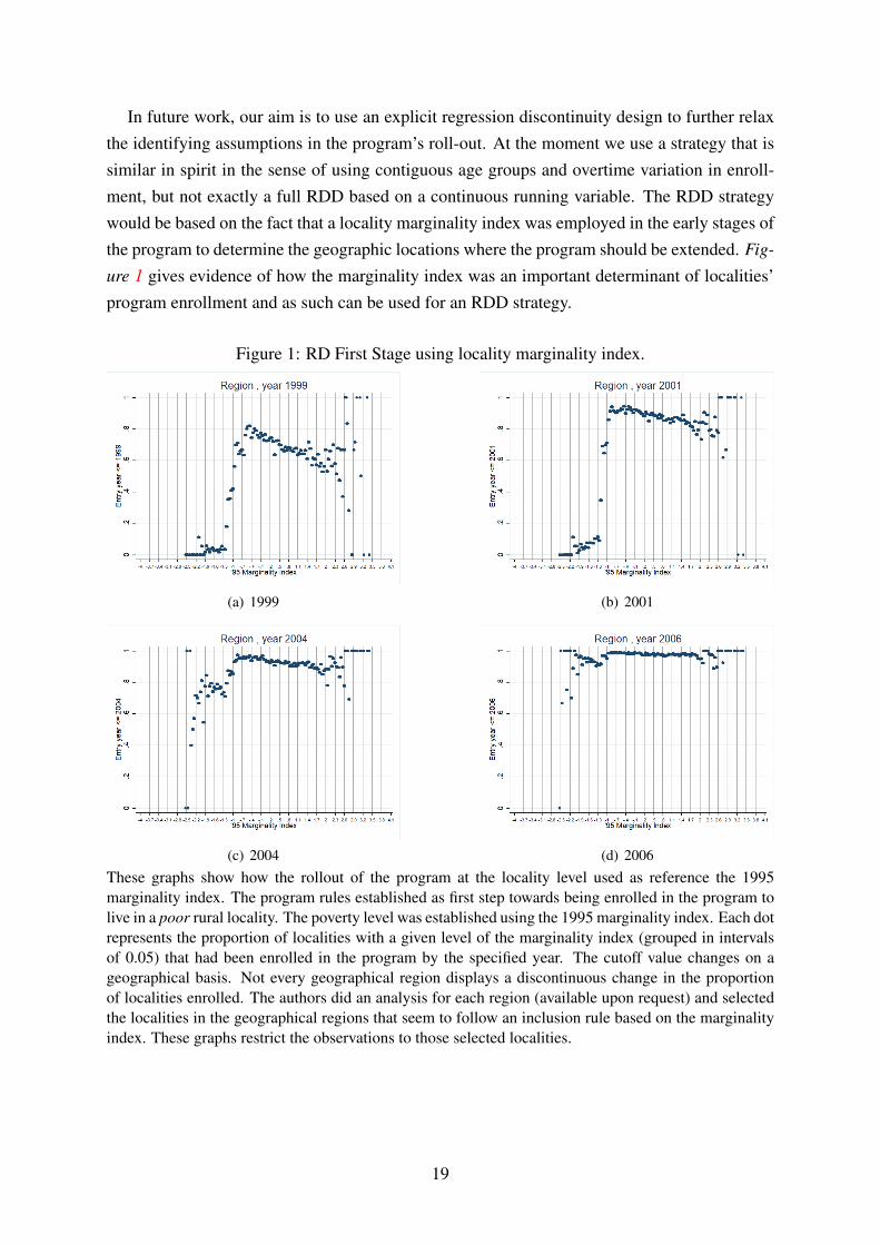
In future work, our aim is to use an explicit regression discontinuity design to further relaxthe identifying assumptions in the program’s roll-out. At the moment we use a strategy that issimilar in spirit in the sense of using contiguous age groups and overtime variation in enroll-ment, but not exactly a full RDD based on a continuous running variable. The RDD strategywould be based on the fact that a locality marginality index was employed in the early stages ofthe program to determine the geographic locations where the program should be extended. Fig-

ure 1 gives evidence of how the marginality index was an important determinant of localities’program enrollment and as such can be used for an RDD strategy.

Figure 1: RD First Stage using locality marginality index.

(a) 1999 (b) 2001

(c) 2004 (d) 2006

These graphs show how the rollout of the program at the locality level used as reference the 1995marginality index. The program rules established as first step towards being enrolled in the program tolive in a poor rural locality. The poverty level was established using the 1995 marginality index. Each dotrepresents the proportion of localities with a given level of the marginality index (grouped in intervalsof 0.05) that had been enrolled in the program by the specified year. The cutoff value changes on ageographical basis. Not every geographical region displays a discontinuous change in the proportionof localities enrolled. The authors did an analysis for each region (available upon request) and selectedthe localities in the geographical regions that seem to follow an inclusion rule based on the marginalityindex. These graphs restrict the observations to those selected localities.

19

VI Results

VI.A Original Experiment

As described above, we begin by analyzing the effects of the early versus late treatment usingthe 1997 original experimental design that assigned 320 of 506 localities to receive governmenttransfers as early as 1998 and all the way to the end of 1999. We estimate equations (1), (2), (3)and present the results in the corresponding panels A to C of Tables 6 and 7. We look at durableassets, imputed non-durable (food, personal products, and clothing) expenditures, further toincome and schooling, as outcomes of interest and to original and new households, respectively,as were defined in section IV. Our interest here is to analyze the durable expenditure behaviorin line with the long-term perspective of the overall report and the original spirit of the program.

VI.A.1 Original Households

Table 6 displays no significant differences for treated vs. control original households in mostcases. The outcomes employed in the analysis are an aggregation (counting) of differentdurable goods, a different aggregation through prices for example would be problematic giventhe large variation in quality and vintage for durable goods. We therefore present a countingexercise on the following assets: (i) transportation, which refers to number of vehicles (cars,vans, motorcycles); (ii) entertainment, which includes TV, radio and sound equipment; (iii)kitchen supplies, which adds number of blenders, refrigerators, microwaves, gas stove or elec-tric grills; (iv) basic housing services, which identifies having firms floor, electricity, drainageand water connection in the property; (v) IT assets, which refers to computers and cellphones;and (vi) IT and entertainment services, which include home phone, internet and pay-TV.17

We note that as some of the IT and IT and Entertainment goods are not available in thebaseline wave (1997) when we produce the analysis for such goods in the DiD and ANCOVAspecifications we use as baseline measures the full aggregation of durables.

In Panel B of Table 6 we perform a testing strategy based on the excess growth of the durablegoods in treated vs. control households; while in Panel C we present a standard ANCOVAspecification, i.e. where we regress follow-up outcomes on treatment and control for baselineoutcomes. The results suggest that in general there are no baseline differences, confirmingthat the initial randomization is still valid and that the random selection of households for thelast follow-up or non-differential attrition rates for the most part, see the coefficients attachedto the Treatment dummy. However, in some of the cases, the treatment dummy (outcome in1997) displays significant, yet negative, differences. The differences resulting from the passingof time (2017 dummy) shows that access to the assets has greatly improved for all items, notsurprisingly given that the two waves are 20 years apart, this signals a general improvement in

17A good-by-good analysis is also available upon request.

20

Table 6: Effects on durable good’s accumulation. Original households.(1) (2) (3) (4) (5) (6) (7)

Transport Entert eq Kitchen sup Basic serv IT items IT serv ln(imp cons)Panel A: Cross-section

Treatment -0.023 0.011 -0.054 -0.002 -0.019 0.020 -0.011(0.023) (0.044) (0.050) (0.048) (0.027) (0.036) (0.011)

Constant 0.289*** 1.380*** 1.804*** 2.709*** 0.738*** 0.236*** 8.713***(0.057) (0.099) (0.121) (0.088) (0.071) (0.075) (0.026)

Observations 4,494 4,494 4,494 4,494 4,494 4,494 4,182

Panel B: DiD 1997-2017

Treatment X 2017 0.006 0.098** 0.066 -0.068 0.082 0.127 0.014(0.027) (0.049) (0.058) (0.077) (0.102) (0.107) (0.011)

Treatment -0.017 -0.103** -0.106** 0.034 -0.158** -0.162** -0.023**(0.012) (0.040) (0.043) (0.063) (0.080) (0.079) (0.009)

2017 0.217*** 0.444*** 1.443*** 1.279*** -0.801*** -1.077*** 0.090***(0.022) (0.038) (0.046) (0.061) (0.078) (0.081) (0.008)

Constant 0.030 0.786*** 0.311*** 1.361*** 1.212*** 1.099*** 8.639***(0.030) (0.079) (0.091) (0.085) (0.104) (0.105) (0.020)

Observations 8,988 8,988 8,988 8,988 8,988 8,988 8,656

Panel C: ANCOVA

Treatment -0.020 0.028 -0.029 -0.002 -0.011 0.026 -0.002(0.022) (0.042) (0.047) (0.046) (0.027) (0.036) (0.010)

Y(97) 0.522*** 0.146*** 0.279*** 0.158*** 0.038*** 0.029** 0.383***(0.077) (0.017) (0.019) (0.018) (0.008) (0.011) (0.032)

Constant 0.295*** 1.287*** 1.731*** 2.504*** 0.704*** 0.210*** 5.401***(0.057) (0.098) (0.116) (0.088) (0.071) (0.075) (0.279)

Observations 4,494 4,494 4,494 4,494 4,494 4,494 4,169Mean T 2017 0.247 1.473 1.928 2.532 0.656 0.426 9.052Mean C 2017 0.241 1.435 1.891 2.497 0.662 0.386 9.041

This table shows the long-term effects of the program on a set of variables that result from aggregating groups of durable assets andhousehold characteristics. Observations are restricted to households from 1997 that were successfully found again in 2017 (originalhouseholds). The outcomes constructed are: (1) Transportation, which adds the number of cars and vans; (2) Entertainment equipment,which gathers under entertainment equipment number of TV, radio and sound equipment; (3) Kitchen supplies, which sums the followingappliances: blender, refrigerator, electric grill, gas stove or microwave oven; (4) Basic services, which consists of the availability of thefollowing services: firm floor, electricity, drainage and water access in the property; (5) IT items, which refer to the number of computersand cellphones; and (6) IT services, which sums the home phone, internet and pay-TV; (7) ln(imp cons), is the imputed measure of non-durable expenditure on food personal products, and clothing. Data employed comes from 1997 ENCASEH and 2017-18 ENCEL. PanelA shows the result from a cross-section estimate which only uses data from 2017. Treatment is a dummy variable that identifies if theobservation belongs to one of the 320 original Progresa RCT treatment localities. Panel B does a DiD estimation with 1997 and 2017 asthe two periods considered. Panel C estimates an ANCOVA, which controls for the pre-existing level of the dependent variable (denoted asY(97)). Controls include (from ENCASEH 1997): HH head age, education, speaking a dialect, HH size, % members under 15, dummiesfor home, productive land and draft animals ownership, and locality marginalization index. Standard errors clustered at the locality level.Asterisks indicate significance at the ***1%, **5%, and *10% level.

21

the lives of the original households. Finally, we find a significant but small difference in theentertainment variable. On non-durable expenditure we find no effects.

Several possible explanations could justify these results. First, as already described, ourtreatment definition means having additional transfers in the first year of the program, whichby now was 20 years ago. These additional resources might have had an effect in the shortand medium term, as several papers and reports have shown. However, such effect might nothave carried through 2017. Second, we are looking at households that also existed in 1997,which means that they are predominately composed of older members and increasingly headedby females. Being mostly focused towards benefiting the next generations, PROSPERA mightyield lower impacts in this older-aged group. Third, the sample might not be large enough toenable researchers to detect statistically significant differences. Fourth, we are using durableassets that in the past have been used to identify eligible (poor) households. This might motivaterespondents not to respond truthfully if they believe that the survey could be used as part ofthe assignment process.18 Fifth, it is notoriously complex to look at durables expendituresas these are infrequent purchases of wide quality variation, the data available so far do notinclude the prices of such purchases; further the available data at this stage do not includenon-durable or food consumption directly, so that we resort to an imputation method whichhas clear advantages but also a number of disadvantages as any imputation. The imputationprocedure is described, as mentioned, in Appendix C. Sixth, the original households mighthave passed on to their offspring some of their assets or savings and therefore we might not seea positive difference with the control households. One should bear in mind that PROSPERA bydesign targets children and therefore it is plausible that the main long-run positive effects arefound among those who were the primary target of the policy in terms of health, nutrition, andschooling. While the original households might have had an initial bump in their incomes, thatwas fairly limited in the original experiment, so that eventually the original control householdmight have caught up. The same does not need to be true for the treated children as some of thecontrol children, given their age and school grades, might not be affected at all by the late rollout of the program in control localities. For example, those children at the margin of droppingout of school who were in the control villages would have dropped our while their counterpartsin treatment villages would have stayed in school.

VI.A.2 New Households

In this section we analyze the effects for durable goods purchase, and imputed consumptionexpenditures, by the new households as previously defined: these are mostly the offspring ofthe original households, potentially those children in 1997 that were the target of the policy. Asthese new households are composed by the direct beneficiaries of the program transfers, they

18With certain regularity PROSPERA gathers a similar survey called ENCASEH, whose purpose is to determineif the households are still in poverty and should stay in the program or not.

22

are perhaps the most interesting group to look at. Importantly, as we describe in Table 4 thenew households are younger (as expected), on average the head of household is 31 years old,and, on average, has about 5 more years of education than their parental households. Furtherthe household size is smaller than that of the original households in 1997 with a size of about4 members compared to 7 members for their parental household. These are in practice younghouseholds with fewer, more educated members. We also note that being an early entrant inPROSPERA is not predictive of receiving PROSPERA transfers in 2017, i.e. both offspring ofearly and late treated households are equally likely to receive PROSPERA in 2017. In Table

7 we present the results for these new households. An important motivation for conducting aseparate analysis for these households, comes from the fact that the program has as one of itsmain purposes breaking the cycle of poverty transmitted from parents to sons and daughters.New households will be mostly composed of members that were children in 1997. For thesehouseholds, the results are more encouraging: in the case of entertainment equipment, kitchensupplies and IT and entertainment services, the effects are positive and significant. Also, thesize of the effect is non-negligible, it represents an increase in durable goods of between 7% and16% of the “control” households. Further, on imputed consumption the effects are positive andsignificant at about a 5% increase in non-durable expenditure, a non-trivial effect consideringthe margin of treatment used here.

Given that we are looking into new households, i.e. households composed by individualswho have moved out of their original households, we need to consider that the household for-mation process might not be purely random. For this reason, in Table 8 we provide evidenceon the strength of such selection mechanism, and we show that the program does not producestrong evidence of motivating young individuals moving out of the parental household on av-erage (column 1 Table 8). In both, treatment and control, the proportion of individuals movingout from home and creating their own new household is 60%. However this average effectmasks a more nuanced behavior when looking at different age groups as we do in column 2,it turns out that very young children (0-5 years old in 1997) tend to remain with the originalhousehold longer, while the older children (11-16 years old in 1997) move out earlier to formtheir own household. Similarly, and importantly for the program, these same older childrenare more likely to migrate outside the locality of birth, in fact given the magnitude of the co-efficients on new household formation and migration it seems that a large fraction of the newhouseholds are formed in different locations than those of the parents. The migration behavioris once more consistent with the human capital accumulation channel, migration being partof it or simply a way to reap the benefits of higher human capital. For these reasons, we testwhether those who migrated chose a large city (Mexico City, Guadalajara, or Monterrey) astypically larger cities provide more opportunities for growth (Moretti 2012; De La Roca andPuga 2017). While this latter test is tentative in nature as it relies upon a selected sample ofmigrants, it would have provided some interesting thoughts, however it appears that there is no

23

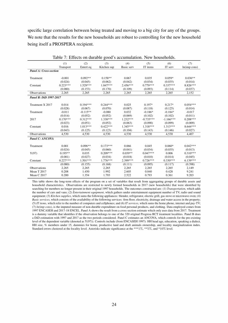
specific large correlation between being treated and moving to a big city for any of the groups.We note that the results for the new households are robust to controlling for the new householdbeing itself a PROSPERA recipient.

Table 7: Effects on durable good’s accumulation. New households.(1) (2) (3) (4) (5) (6) (7)

Transport Entert eq Kitchen sup Basic serv IT items IT serv ln(imp cons)Panel A: Cross-section

Treatment -0.001 0.092** 0.158** 0.067 0.035 0.059* 0.036**(0.024) (0.045) (0.062) (0.042) (0.034) (0.035) (0.014)

Constant 0.223*** 1.529*** 1.847*** 2.456*** 0.779*** 0.337*** 8.826***(0.080) (0.153) (0.170) (0.109) (0.093) (0.114) (0.037)

Observations 2,265 2,265 2,265 2,265 2,265 2,265 2,152

Panel B: DiD 1997-2017

Treatment X 2017 0.014 0.194*** 0.244*** 0.025 0.197* 0.217* 0.054***(0.028) (0.067) (0.070) (0.087) (0.118) (0.125) (0.014)

Treatment -0.011 -0.115** -0.080 0.032 -0.186* -0.184* -0.017(0.014) (0.052) (0.052) (0.069) (0.102) (0.102) (0.011)

2017 0.170*** 0.312*** 1.338*** 1.232*** -0.735*** -1.166*** 0.208***(0.023) (0.051) (0.052) (0.063) (0.090) (0.099) (0.009)

Constant 0.016 1.013*** 0.422*** 1.345*** 1.318*** 1.313*** 8.644***(0.043) (0.125) (0.123) (0.104) (0.143) (0.146) (0.027)

Observations 4,530 4,530 4,530 4,530 4,530 4,530 4,407

Panel C: ANCOVA

Treatment 0.001 0.096** 0.173*** 0.066 0.045 0.060* 0.042***(0.024) (0.045) (0.060) (0.041) (0.034) (0.035) (0.013)

Y(97) 0.195** 0.035 0.209*** 0.039** 0.047*** 0.006 0.310***(0.081) (0.027) (0.034) (0.018) (0.010) (0.014) (0.045)

Constant 0.227*** 1.501*** 1.776*** 2.399*** 0.726*** 0.330*** 6.139***(0.080) (0.155) (0.168) (0.111) (0.095) (0.117) (0.398)

Observations 2,265 2,265 2,265 2,265 2,265 2,265 2,149Mean T 2017 0.208 1.450 1.992 2.605 0.840 0.428 9.241Mean C 2017 0.200 1.354 1.793 2.522 0.793 0.361 9.203

This table shows the long-term effects of the program on a set of variables that result from aggregating groups of durable assets andhousehold characteristics. Observations are restricted to newly formed households in 2017 (new households) that were identified bysearching for members no longer present in their original 1997 households. The outcomes constructed are: (1) Transportation, which addsthe number of cars and vans; (2) Entertainment equipment, which gathers under entertainment equipment number of TV, radio and soundequipment; (3) Kitchen supplies, which sums the following appliances: blender, refrigerator, electric grill, gas stove or microwave oven; (4)Basic services, which consists of the availability of the following services: firm floor, electricity, drainage and water access in the property;(5) IT items, which refer to the number of computers and cellphones; and (6) IT services, which sums the home phone, internet and pay-TV;(7) ln(imp cons), is the imputed measure of non-durable expenditure on food personal products, and clothing. Data employed comes from1997 ENCASEH and 2017-18 ENCEL. Panel A shows the result from a cross-section estimate which only uses data from 2017. Treatmentis a dummy variable that identifies if the observation belongs to one of the 320 original Progresa RCT treatment localities. Panel B doesa DiD estimation with 1997 and 2017 as the two periods considered. Panel C estimates an ANCOVA, which controls for the pre-existinglevel of the dependent variable (denoted as Y(97)). Controls include (from ENCASEH 1997): HH head age, education, speaking a dialect,HH size, % members under 15, dummies for home, productive land and draft animals ownership, and locality marginalization index.Standard errors clustered at the locality level. Asterisks indicate significance at the ***1%, **5%, and *10% level.

24

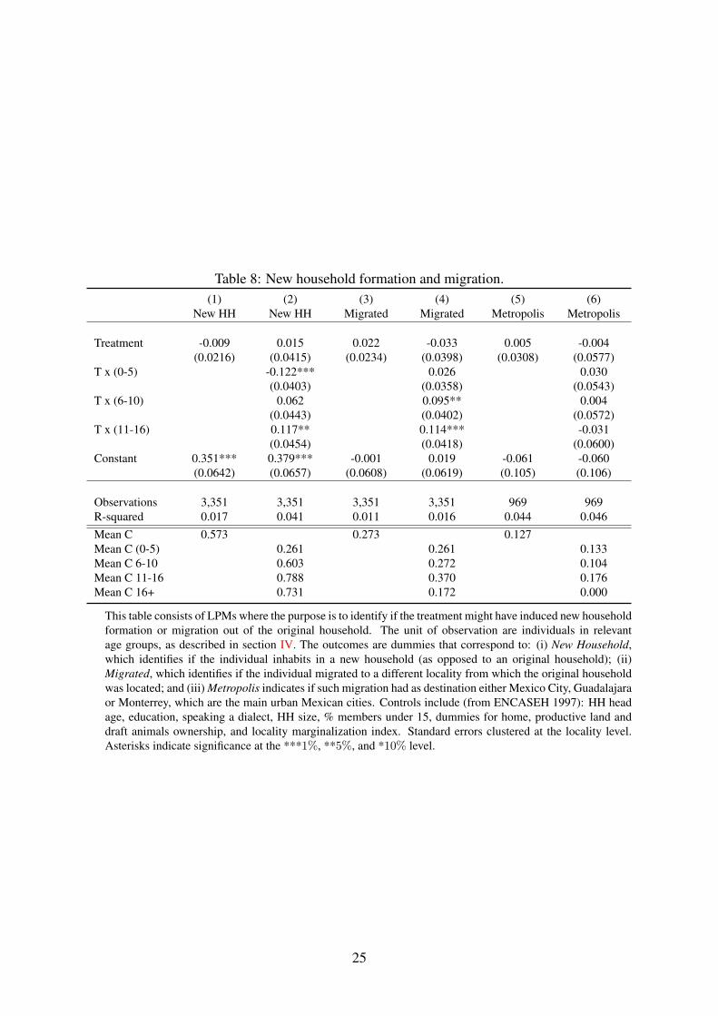
Table 8: New household formation and migration.(1) (2) (3) (4) (5) (6)

New HH New HH Migrated Migrated Metropolis Metropolis

Treatment -0.009 0.015 0.022 -0.033 0.005 -0.004(0.0216) (0.0415) (0.0234) (0.0398) (0.0308) (0.0577)

T x (0-5) -0.122*** 0.026 0.030(0.0403) (0.0358) (0.0543)

T x (6-10) 0.062 0.095** 0.004(0.0443) (0.0402) (0.0572)

T x (11-16) 0.117** 0.114*** -0.031(0.0454) (0.0418) (0.0600)

Constant 0.351*** 0.379*** -0.001 0.019 -0.061 -0.060(0.0642) (0.0657) (0.0608) (0.0619) (0.105) (0.106)

Observations 3,351 3,351 3,351 3,351 969 969R-squared 0.017 0.041 0.011 0.016 0.044 0.046Mean C 0.573 0.273 0.127Mean C (0-5) 0.261 0.261 0.133Mean C 6-10 0.603 0.272 0.104Mean C 11-16 0.788 0.370 0.176Mean C 16+ 0.731 0.172 0.000

This table consists of LPMs where the purpose is to identify if the treatment might have induced new householdformation or migration out of the original household. The unit of observation are individuals in relevantage groups, as described in section IV. The outcomes are dummies that correspond to: (i) New Household,which identifies if the individual inhabits in a new household (as opposed to an original household); (ii)Migrated, which identifies if the individual migrated to a different locality from which the original householdwas located; and (iii) Metropolis indicates if such migration had as destination either Mexico City, Guadalajaraor Monterrey, which are the main urban Mexican cities. Controls include (from ENCASEH 1997): HH headage, education, speaking a dialect, HH size, % members under 15, dummies for home, productive land anddraft animals ownership, and locality marginalization index. Standard errors clustered at the locality level.Asterisks indicate significance at the ***1%, **5%, and *10% level.

25

VI.A.3 Re-weighted Estimates

Table 9 shows the results from re-weighting the observations in the sample in order to replicatethe results that would have been obtained without attrition. Given that attrition occurred indifferent forms, we produce three different comparisons. The method employed for the re-weighting is the inverse probability weighting (DiNardo et al., 1996). As a first step, a logitmodel of attrition with respect to a group of variables is estimated. All the observations areemployed at this stage since baseline explanatory variables from the 1997 ENCASEH are usedto predict attrition. Based on the results of this logit, a weighting factor is calculated to be usedwith the analysis sample from the previous estimations.

Table 9: Re-weighted estimates of long-term effects on durable good’s accumulation.(1) (2) (3) (4) (5) (6) (7)

Transport Entert eq Kitchen sup Basic serv IT items IT serv ln(imp cons)Panel A: Original Households

1. Analysis SampleTreatment -0.020 0.028 -0.029 -0.002 -0.011 0.026 -0.002

(0.022) (0.042) (0.047) (0.046) (0.027) (0.036) (0.010)Observations 4,494 4,494 4,494 4,494 4,494 4,494 4,169

2. Original DistributionTreatment -0.016 -0.002 -0.025 -0.004 -0.011 0.029 -0.005

(0.021) (0.043) (0.047) (0.049) (0.028) (0.033) (0.010)Observations 4,471 4,471 4,471 4,471 4,471 4,471 4,150

3. Localities 2017 distributionTreatment -0.016 -0.001 -0.027 -0.004 -0.014 0.033 -0.005

(0.021) (0.043) (0.047) (0.048) (0.028) (0.033) (0.010)Observations 4,471 4,471 4,471 4,471 4,471 4,471 4,150Mean T 2017 0.247 1.473 1.928 2.532 0.656 0.426 9.052Mean C 2017 0.241 1.435 1.891 2.497 0.662 0.386 9.041

Panel B: New Households

1. Analysis SampleTreatment 0.001 0.096** 0.173*** 0.066 0.045 0.060* 0.042***

(0.024) (0.045) (0.060) (0.041) (0.034) (0.035) (0.013)Observations 2,265 2,265 2,265 2,265 2,265 2,265 2,149

2. Localities 2017 distributionTreatment -0.005 0.076 0.144** 0.052 0.041 0.054 0.040***

(0.026) (0.049) (0.065) (0.043) (0.036) (0.037) (0.013)Observations 1,912 1,912 1,912 1,912 1,912 1,912 1,822Mean T 2017 0.208 1.450 1.992 2.605 0.840 0.428 9.241Mean C 2017 0.200 1.354 1.793 2.522 0.793 0.361 9.203

This table shows the long-term effects of the program on a set of variables that result from aggregating groups of durable assets andhousehold characteristics. The reweighting strategy employed is the inverse probability weight (DiNardo et al., 1996). In Panel A ob-servations are restricted to households included in 1997 ENCASEH (original households), while in Panel B observations are restrictedto newly formed households in 2017 (new households) that were identified by searching for members no longer present in their original1997 households. The reweighting strategy seeks to reproduce the original sample distribution. Two different target distributions are setfollowing the attrition analysis done in Table 3. Original Distribution means the 1997 sample, which corresponds to the original house-holds in the 506 localities. The purpose is to make our results comparable to the vast literature that focuses on this group. Localities2017 distribution is based on the 334 localities chosen for the sample and assumes that all the original 1997 households in those localitieswould have been found. The outcomes employed are: (1) Transportation, which adds the number of cars and vans; (2) Entertainmentequipment, which gathers under entertainment equipment number of TV, radio and sound equipment; (3) Kitchen supplies, which sums thefollowing appliances: blender, refrigerator, electric grill, gas stove or microwave oven; (4) Basic services, which consists of the availabilityof the following services: firm floor, electricity, drainage and water access in the property; (5) IT items, which refer to the number ofcomputers and cellphones; and (6) IT services, which sums the home phone, internet and pay-TV; (7) ln(imp cons), is the imputed measureof non-durable expenditure on food personal products, and clothing. Data employed comes from 1997 ENCASEH and 2017-18 ENCEL.The table shows the results from an ANCOVA estimate, which controls for the pre-existing level of the dependent variable (denoted asY(97)). Controls include (from ENCASEH 1997): HH head age, education, speaking a dialect, HH size, % members under 15, dummiesfor home, productive land and draft animals ownership, and locality marginalization index. Standard errors clustered at the locality level.Asterisks indicate significance at the ***1%, **5%, and *10% level.

26

Panel A refers to original households. Two sources of attrition are considered, as describedin section IV.A: (i) localities composition, which means that just a sub-sample of the 506 orig-inal localities was surveyed; and (ii) response attrition, which means that some households inthe selected localities were not found. In the first part of Panel A (Analysis sample) we showthe main results estimated with the ANCOVA for original households for comparative reasons.Next, we show the results if no attrition happened (Original distribution). This results corre-spond to the household distribution in 506 and we add it for comparative reasons with respectto the original literature about the program. The reweighting factor employed for this resultis the one included in column (1) of Table 3. As can be seen, no significant effects on assetaccumulation are obtained for this reweighted sample. Afterwards, in the third part of Panel A,we show the results that would be obtained if we only control for the response attrition. Thatis, the purpose is to replicate the distribution of all the households in the selected 334 localities.The reweighting factor in this case corresponds to column (3) of Table 3. Again, no significanteffects in asset accumulation are found. These results were expected since the attrition analysissuggested that no differential attrition between treatment groups was found.

Panel B refers to the new households. For this group attrition seems to be more relevant.Attrition here refers to the impossibility of finding all the individuals in the relevant age groupsthat exited their households to form a new one (or joined another household). Columns (5)and (6) in Table 3 show the attrition analysis for this group. To start with, a small proportionof individuals was found (40%). Second, the attrition analysis shows some slight significantdifferences between treatment and control (the joint test with the interaction terms has a p-value of 0.075). For this reason, we perform the reweighting strategy using the results fromcolumn (6) where the interaction terms were included. This reweighting factor would replicatethe household distribution that would result if all the individuals in the relevant age groupsthat moved out of their original household were found in their new household. The results areshown in comparison to the main ANCOVA results (Analysis sample). As can be seen in thetable, the results in asset accumulation are very similar to the resulting analysis with the samplefound.

VI.B Youths and Intergenerational Transmission

It is paramount when looking at long-term effects of such an important program to look at thelife-cycle as well as at the intergenerational effects, ultimately the long-term success of thepolicy will be based on the success of the offspring of the originally treated households or thechildren who directly benefited from the government transfers as well as the other componentsof the program.

27

VI.B.1 Effects in the Relevant Age Group

To better explore the effects on the sample of individuals that form the “next generation”, wetake the individuals classified in the group of interest, given their age. Recall, that this includesindividuals who in 1997 were newborn, just beginning school or at sixth grade. For example, ifwe look at the effects of PROSPERA for those who benefit from the policy over their life, we arelooking at the effect of exposure to the policy on their lifecycle outcomes. Relatedly, we couldbe interested in understanding whether the offspring of original households who are themselvesbeneficiaries of the transfers are faring better than their parents. This latter would be looking atintergenerational mobility and transmission of income, human capital, and consumption. Bothdimensions are rather important as the lifecycle view will investigate whether being treated atan earlier stage of life could have long-lasting consequences (as in Hoddinott et al. 2008 andMartorell 2017); in the intergenerational view that is addressing the link between parents andoffspring and how PROSPERA can foster upward mobility in society by improving the lives ofthe next generation with respect to those of their parents.

Table 10 suggests that it is this group of individuals driving the positive results for the newhouseholds, since entertainment equipment, kitchen supplies, and non-durable expenditure dis-play significant effects in this analysis with similar magnitudes to those previously found. PanelB explores the heterogeneity of the effects distinguishing between young members still livingin the original household and those that formed their household. This analysis confirms ourprevious hypothesis: it is the case that the young members that formed their own householdssignificantly benefit from the program. Panel C also indicates that age-wise, the individualsdriving the positive results correspond to those who were 11 to 16 in 1997 (i.e. those in theircritical stages of schooling, where dropout rates were more common).

Importantly, this latter analysis confirms that those children at risk of dropping out of sec-ondary schooling were in fact retained because of the program, those are the individuals aged11-16 in 1997, and we find sustained positive effects in durable purchases and all other out-comes exactly for this group. However, we should stress that there is also redistribution ofresources within the household as also older children in 1997 those older than 16, who for thelarge part were excluded from the direct schooling transfers as too old, seem to have bene-fited with respect to their control counterpart, certainly in terms of kitchen durables but also(albeit not significant) in the other durable categories. Here we note that, as evidence of thedirect channel through improved human capital, the schooling results and partly the effect onincome (not significantly different from zero) build a direct connection between the policy andits long-term effects. In Panel D, we investigate whether PROSPERA provided some insuranceagainst health shocks of the head of household, we find that the positive effects of PROSPERAon durables and non-durables are somewhat also present for those households who suffered ahealth shock (albeit insignificant and less robust), one should point out here that health shocks

28

Table 10: Heterogeneous effects of PROSPERA on young members.(1) (2) (3) (4) (5) (6) (7) (8)

Transport Enterteq

Kitchensup

Basicserv

Y.school

Inc > 0 log(income)ln(impcons)

Panel A: Overall

Treatment X 2017 0.0275 0.119* 0.142** -0.0119 0.0269 -0.0194 -0.0736 0.0311***(0.0272) (0.0609) (0.0593) (0.0820) (0.209) (0.0273) (0.0848) (0.0119)

Panel B: Household status

Original HH 0.050 0.043 -0.007 -0.042 0.221 -0.062* -0.113 0.001(0.039) (0.072) (0.072) (0.090) (0.261) (0.038) (0.094) (0.014)

New HH 0.009 0.174** 0.253*** 0.011 -0.130 0.028 -0.046 0.054***(0.029) (0.069) (0.072) (0.088) (0.237) (0.027) (0.100) (0.014)

Panel C: Age (in 1997) groups

0-5 0.025 0.072 0.148** -0.035 0.200 -0.009 -0.043 0.022(0.032) (0.075) (0.072) (0.089) (0.220) (0.035) (0.065) (0.015)

6-10 -0.001 0.108 0.019 -0.001 0.167 -0.013 -0.070 0.031*(0.036) (0.091) (0.085) (0.100) (0.258) (0.036) (0.058) (0.018)

11-16 0.057 0.329*** 0.262** -0.017 0.711*** -0.016 0.097 0.050**(0.048) (0.101) (0.112) (0.131) (0.252) (0.052) (0.166) (0.021)

Over 16 0.097 0.051 0.307** 0.130 -0.043 -0.023 0.187 0.045(0.060) (0.147) (0.154) (0.137) (0.293) (0.087) (0.171) (0.034)

Panel D: Health shocks

No health shocks 0.026 0.178*** 0.148** 0.002 0.041 -0.047 -0.122 0.033***(0.030) (0.068) (0.066) (0.086) (0.228) (0.031) (0.092) (0.013)

Health shocks 0.031 -0.038 0.127 -0.103 -0.010 0.047 0.052 0.027(0.038) (0.078) (0.081) (0.100) (0.293) (0.039) (0.110) (0.018)

Panel E: Migration

Same locality 0.043 0.061 0.074 -0.056 -0.086 -0.035 -0.057 0.013(0.031) (0.068) (0.068) (0.087) (0.232) (0.032) (0.102) (0.012)

Mig: Metropolis 0.047 0.477** -0.043 0.225 0.603 0.031 -0.176 0.047(0.063) (0.225) (0.2142) (0.239) (0.986) (0.045) (0.224) (0.043)

Mig: Other -0.017 0.227** 0.314*** 0.055 0.226 0.007 -0.184 0.061(0.042) (0.092) (0.098) (0.112) (0.311) (0.032) (0.110) (0.020)

Observations 6,702 6,702 6,702 6,702 6,702 5,484 4,794 6,527Mean C 1997 0.020 0.985 0.412 1.218 1.392 0.036 0.237 8.971Mean C 2017 0.220 1.420 1.814 2.483 8.009 0.799 8.118 9.139

This table shows the possible heterogeneity of the long-term effect for individuals by specific groups of inter-est. The unit of observation is an individual, who could be in an original or new household. The outcomesconstructed are: (1) Transportation, which adds the number of cars and vans; (2) Entertainment equipment,which gathers under entertainment equipment number of TV, radio and sound equipment; (3) Kitchen sup-plies, which sums the following appliances: blender, refrigerator, electric grill, gas stove or microwave oven;(4) Basic services, which consists of the availability of the following services: firm floor, electricity, drainageand water access in the property; (5) Years of completed formal schooling; (6) Pos income indicates house-hold per capita income greater than zero; (7) log(income), is total individual income; and (8) log(imp cons),is the imputed measure of non-durable expenditure on food personal products, and clothing. Data employedcomes from 1997 ENCASEH and 2017-18 ENCEL. Panel A shows a DiD estimation. Panel B estimates thetreatment effect for different HH types: original and new. Panel C explores differences in the treatment effectby groups of age formed based on the ages associated to critical schooling stages. Panel D shows differencesby health shocks status (health shocks are defined as having at least one household member sick or injuredduring the two weeks before the survey). Panel E looks into the treatment effect by migration status (Metropo-lis includes Mexico City, Guadalajara and Monterrey). Controls include (from ENCASEH 1997): HH headage, education, speaking a dialect, HH size, % members under 15, dummies for home, productive land anddraft animals ownership, and locality marginalization index. Standard errors clustered at the locality level.Asterisks indicate significance at the ***1%, **5%, and *10% level.

29

are seldom fully exogenous so that this is just a tentative correlation analysis. Finally, as shownin Panel E, the positive effects are driven mostly by migrants (but migrants not to the big cities).Interestingly, it seems to be the case that these individuals are doing better in terms of durableassets, but not in income.

VI.B.2 Intergenerational Transmission

In Table 11 we show the effects of PROSPERA on intergenerational mobility in terms of di-vergence of children’s outcomes from their parents, perhaps one of the most relevant aspectof a long-term evaluation. For the new generation, the offspring, still living at home we findrelatively little aside from a closing of the gap more pronounced for treated households in termsof income percentile. More interestingly for the newly formed households in Panel B, we findsubstantial evidence of improvement in the rankings of education, asset holding and incomedistribution; in fact the results suggest that PROSPERA also improved the general mobility sothat not only the children of the better off original households appear to do better but particu-larly those who started lower in the distribution seem to do better (see the negative sign on theTreat *Y (G1) coefficient). These effects are economically relevant and quite encouraging asthey show an upward mobility for the beneficiaries, exactly what the program aimed to achieve.

30

Table 11: Intergenerational transmission. Convergence / Divergence.Years school Asset index Pctile Income Pctile

(1) (2) (3) (4) (5) (6)∆Y ∆Y ∆Y ∆Y ∆Y ∆Y

Panel A: Original households

Treat -0.282 -0.0788 1.892 -3.000 0.889 -7.220*(0.219) (0.337) (1.858) (2.521) (2.965) (3.830)

Y (G1)1997 -0.657*** -0.681*** -0.997***(0.0636) (0.0457) (0.0564)

Treat ∗ Y (G1)1997 -0.031 0.092* 0.113(0.0723) (0.0520) (0.0746)

Constant 1.270* 6.942*** 2.515 38.73*** 59.71*** 93.42***(0.679) (0.717) (6.794) (5.755) (8.744) (7.655)

Observations 1,442 1,442 1,432 1,432 939 939R-squared 0.056 0.266 0.027 0.275 0.081 0.486Mean C Y (G1)1997 2.86 2.86 37.00 37.00 44.24 44.24Mean C Y (G2)2017 8.32 8.32 45.04 45.04 56.08 56.08

Panel B: New households

Treat 0.298 0.833*** 6.918*** 4.035 5.950** 6.579*(0.192) (0.270) (2.269) (2.860) (2.549) (3.629)

Y (G1)1997 -0.657*** -0.862*** -0.833***(0.0469) (0.0436) (0.0524)

Treat ∗ Y (G1)1997 -0.139** 0.014 -0.078(0.0555) (0.0572) (0.0644)

Constant 4.061*** 8.173*** -16.51** 30.07*** 11.61 55.85***(0.705) (0.625) (6.932) (5.891) (9.296) (7.894)

Observations 1,891 1,891 1,880 1,880 1,354 1,354R-squared 0.089 0.391 0.054 0.357 0.069 0.423Mean C Y (G1)1997 2.71 2.71 38.89 38.89 42.46 42.46Mean C Y (G2)2017 7.76 7.76 40.51 40.51 42.36 42.36

This table analyzes the inter-generational mobility relation to the parent’s (Generation 1, G1) distributionalposition to understand how poorer or richer households manage to change their distributional position forspecific outcomes and how Treatment affects this relation. Inter-generational mobility is defined as ∆ Y =Y (G2)2017 − Y (G1)1997, where Y (G2)2017 and Y (G1)1997 are defined as the outcome of the offspring (G2)or parents (G1) observed in 2017 or 1997, respectively. The outcomes of interest considered are: (1) yearsof schooling; (2) a durable asset index formed with a principal component that considers ownership of cars,vans, TV, radio, sound equipment, blender, refrigerator, electric grill, gas stove, microwave oven, firm floor,electricity, drainage and water access in the property; and (3) monthly income. For column (1) the levelof years of schooling is used by itself. For columns (2) and (3), the percentile of each outcome is calculatedrelative to all the individuals inside the same 10-year window age range. The unit of observation are individualsin relevant age groups, as described in section IV and their parents. Controls include (from ENCASEH 1997):HH head age, education, speaking a dialect, HH size, % members under 15, dummies for home, productiveland and draft animals ownership, and locality marginalization index. Standard errors clustered at the localitylevel. Asterisks indicate significance at the ***1%, **5%, and *10% level.

31

VI.C DiD Estimates of Program Roll-out

Our second identification strategy, based on the sequential roll-out of the policy, provides ad-ditional evidence and on larger differences in exposure to the program than the experimentalvariation discussed so far. At the same time, the data employed in this part contain directmeasures of food security and vulnerability which add another layer to our welfare analysis.Further to that, we can also test for the effect of PROSPERA on later dependency on govern-mental programs, this would be a test of a successful policy able to graduate its beneficiariesout of social programs. Our approach here is to produce DiD estimates similarly to Parker andVogl (2018), but with INEGI’s 2015 intercensus data.19 Figure 2 contains the main estimatesof this strategy. Each sub-graph shows the τ estimates from equation (5), which correspond todifference-in-difference estimates. As one moves to the right through the X-axis you increasethe exposure to PROSPERA (calculated by comparing 1998 to different delays to enroll) for agiven cohort with respect to the cohort that should not be benefited by the program (17-22 yearold individuals in 2001).

The results show positive effects on education, particularly for the cohort with the youngestmembers, which increases their schooling attainment between 0.5 and 1.5 additional years. Forthe other cohorts, the program involves an increase around 0.5 years of schooling. Regard-ing income, positive and significant effects are found: household per capita income increasesbetween 2% and 8%, with largest effects for the cohort of those aged 6-10 in 2001. Positiveeffects are also found for a composite index of house characteristics and durable assets. Whenanalyzing asset by asset, the largest effects are found for type of floor, washer, and cellphone.The largest effects are again found for the youngest cohort. To test for dependency on govern-ment aid, or graduation from social programs, we use, as dependent variable, a dummy equalto 1 if the household receives transfers from the government. In this case, overall the evidencesuggests that longer exposure to PROSPERA decreases the dependency on government aid.Unfortunately, this measure does not distinguish PROSPERA from other type of governmentaid. Finally, we look at proxies for vulnerability and food security: two different measuresdirectly addressing food consumption. One question asks whether any adult, in the household,went hungry at least once during the last month. The second question asks whether not enoughmoney was available to purchase enough food variety. We take these two questions as prox-ies for food security, vulnerability, and quality of the diet. For the younger cohorts we havepositive effects on this measure of food security, as those exposed longer are less likely to gohungry (although the estimates are not precise). As for food variety, larger effects are found forthe youngest cohort. For them, the likelihood of not being able to buy enough variety decreasesbetween 1 and 2 percentage points for those with longer exposure.20 These latter two effects on

19As explained in section V.B, these estimates are part of our current research where we seek to use an RDDdesign with the original rule that established that participating localities would be enrolled to the program basedon a marginality index.

20The food scarcity variables are separately asked for children and adults in the household. Similar estimates

32

Figure 2: DiD estimates using program’s rollout by age cohorts.

These graphs show DiD estimates of the rollout of the program for the different cohorts. The coefficientsplotted correspond to the τ ’s in equation (5). Each dot in the graph should be interpreted as the effect ofadditional years of exposure to the program for a specific cohort. To form the X-axis, years of exposureare calculated by comparing entering in 1998 with respect to entering in different years. Therefore,additional 1-3 years implies that the comparison localities in this classification entered between 1999and 2001; additional 4-7 years compares with respect to entering between 2002 and 2005; and finally,8+ years of additional exposure means comparing with the localities that enrolled after 2006. Cohort C4,which corresponds to individuals aged 17-22 in 2001 is taken as a reference to control for the selectioninto early versus late treatment. The outcomes used are: (1) years of schooling, (2) log of household’sper capita income, (3) a PCA index using durable household assets, (4) dummy indicating if householdreceives government transfers, (5) dummy indicating if any adult in the household went hungry somedaylast month, and (6) dummy indicating if adults in the household were not able to eat enough food variety.The cohorts used in the graphs were constructed using individual’s age in 2001: (C1) ages 0-5, whichcorresponds to the gray line, (C2) ages 6-10, which corresponds to the green line and (C3) ages 11-16,which corresponds to the blue line. Filled dots • are significant at the 5% level, unfilled dots ◦ aresignificant at the 10% level and unfilled triangles4 are non-significant estimates. Standard errors wereclustered at the locality level. Data used for these estimations comes from the 2015 INEGI intercensus.

33

food security, coupled with the results on aid dependency, suggest that a higher exposure forthose most likely to benefit from PROSPERA, with respect to their control counterpart, movedbeneficiaries on a higher welfare path. There are clearly some limitations to this approach, notdifferently from other studies employing DiD strategies. For instance, if more capable individ-uals from younger cohorts migrate out of poorer locations to a larger extent, our results mightreflect a self-selection problem. Parker and Vogl (2018) provide some robustness checks for theselective migration by using each individual’s previous location and noting that PROSPERAdoes not seem to promote migration in large numbers.21

VII Conclusions

We provide an analysis of PROSPERA’s ability to improve the social and economic lives oforiginal households and their offspring. We do so through the lens of the long-term effectsof the program on the welfare of its recipients. While the study has some limitations dueto the available data, as well as the limited extent of variation in treatment intensity (for thecleanest identification strategy), the long-term effects of PROSPERA are particularly encour-aging for the offspring of the originally treated households. These new households, formedby young adults who were themselves direct beneficiaries of the program (when children),present higher ownership of durable assets, and larger non-durable consumption expenditure,suggesting higher welfare. These results are fully consistent with the improved human capital,through the schooling and health effects well documented by the literature on PROSPERA’sshort and medium-term effects. Even more importantly, these new households are climbingthe economic and social ladder faster than their control counterpart. Their rank, in the relevantdistribution, is certainly higher than their parents’ in terms of asset holdings and income, anddifferentially so for the offspring of the early entrants in PROSPERA. We take this latter resultas very exciting evidence of PROSPERA’s ability to put beneficiaries on a positive trajectoryand permanently out of poverty. Our results are fully consistent with the existing literature,given the improvements in human capital (health and education), accompanied by higher, andless volatile, income streams through savings and investment in higher returns activities. Ul-timately, the success of PROSPERA should be judged upon its long-term (and permanent)effects and on its ability to lift beneficiaries, and their offspring, out of poverty, facilitatingtheir upward mobility on the social and economic ladder. The future direction for these studiesis that of acquiring larger and more detailed data to be able to augment the current evidencewith other indicators, including directly measuring non-durable consumption, and providinga better understanding of the exact mechanisms behind our findings with the aid of a formaltheoretical framework.

as the ones presented for adults are found for children.21Further work is being done by the authors at the time of writing to tackle these concerns.

34

ReferencesABEYASEKERA, S. AND P. WARD (2002): “Models for Predicting Expenditure per Adult

Equivalent,” Unpublished.

ADHVARYU, A., A. NYSHADHAM, T. MOLINA, AND J. TAMAYO (2018): “Helping ChildrenCatch Up: Early Life Shocks and the PROGRESA Experiment,” Working Paper 24848,National Bureau of Economic Research.

AIZER, A., S. ELI, J. FERRIE, AND A. LLERAS-MUNEY (2016): “The Long-Run Impact ofCash Transfers to Poor Families,” American Economic Review, 106, 935–71.

ANGELUCCI, M. AND G. DE GIORGI (2009): “Indirect Effects of an Aid Program: How DoCash Transfers Affect Ineligibles’ Consumption?” American Economic Review, 99, 486–508.

ANGELUCCI, M., G. DE GIORGI, M. RANGEL, AND I. RASUL (2010): “Family networksand school enrolment: Evidence from a randomized social experiment,” Journal of Public

Economics, 94, 197 – 221.

ANGELUCCI, M., G. DE GIORGI, AND I. RASUL (2017): “Consumption and Investment inResource Pooling Family Networks,” The Economic Journal.

ATKINSON, A. (2011): “The Restoration of Welfare Economics,” American Economic Review,101, 157–161.

ATTANASIO, O., V. DI MARO, V. LECHENE, AND D. PHILLIPS (2013): “Welfare conse-quences of food prices increases: Evidence from rural Mexico,” Journal of Development

Economics, 104, 136 – 151.

ATTANASIO, O. AND V. LECHENE (2002): “Tests of Income Pooling in Household Decisions,”Review of Economic Dynamics, 5, 720–748.

ATTANASIO, O., C. MEGHIR, AND A. SANTIAGO (2012): “Education Choices in Mexico:Using a Structural Model and a Randomized Experiment to Evaluate PROGRESA,” The

Review of Economic Studies, 79, 37–66.

ATTANASIO, O. P. AND V. LECHENE (2014): “Efficient Responses to Targeted Cash Trans-fers,” Journal of Political Economy, 122, 178–222.

ATTANASIO, O. P. AND L. PISTAFERRI (2016): “Consumption Inequality,” Journal of Eco-

nomic Perspectives, 30, 3–28.

BAEZ, J. AND A. CAMACHO (2011): Assessing the long-term effects of conditional cash trans-

fers on human capital : evidence from Colombia, WPS 5681.

35

BAIRD, S., C. MCINTOSH, AND B. OZLER (2011): “Cash or Condition? Evidence from aCash Transfer Experiment *,” The Quarterly Journal of Economics, 126, 1709–1753.

BANERJEE, A. AND E. DUFLO (2011): Poor economics: a radical rethinking of the way to

fight global poverty, Public Affairs.

BARHAM, T., K. MACOURS, AND J. MALUCCIO (2017): “Are Conditional Cash TransfersFulfilling Their Promise? Schooling, Learning, and Earnings After 10 Years,” .

BARRERA-OSORIO, F., L. LINDEN, AND J. SAAVEDRA (2017): “Medium- and Long-TermEducational Consequences of Alternative Conditional Cash Transfer Designs: ExperimentalEvidence from Colombia,” .

BEHRMAN, J., S. PARKER, AND P. TODD (2011): “Do Conditional Cash Transfers for School-ing Generate Lasting Benefits?: A Five-Year Followup of PROGRESA/Oportunidades,”Journal of Human Resources, 46, 93–122.

BIANCHI, M. AND M. BOBBA (2010): “”Financial Constraints and Occupational Choices:Evidence from Rural Mexico”,” Unpublished.

BLUNDELL, R., L. PISTAFERRI, AND I. PRESTON (2005): “Imputing consumption in thePSID using food demand estimates from the CEX,” .

——— (2008): “Consumption Inequality and Partial Insurance,” American Economic Review,98, 1887–1921.

BOBONIS, G., R. CASTRO, AND J. MORALES (2015): “”Conditional Cash Transfers forWomen and Spousal Violence: Evidence of the Long-Term Relationship from the Opor-tunidades Program in Rural Mexico,” .

BOBONIS, G. J. (2009): “Is the Allocation of Resources within the Household Efficient? NewEvidence from a Randomized Experiment,” Journal of Political Economy, 117, 453–503.

BURSZTYN, L. AND L. C. COFFMAN (2012): “The Schooling Decision: Family Preferences,Intergenerational Conflict, and Moral Hazard in the Brazilian Favelas,” Journal of Political

Economy, 120, 359–397.

CHETTY, R., N. HENDREN, P. KLINE, AND E. SAEZ (2014): “Where is the land of oppor-tunity? The geography of intergenerational mobility in the United States,” The Quarterly

Journal of Economics, 129, 1553–1623.

CUNHA, J., G. DE GIORGI, AND S. JAYACHANDRAN (2018): “The Price Effects of CashVersus In-Kind Transfers,” The Review of Economic Studies.

DE LA ROCA, J. AND D. PUGA (2017): “Learning by Working in Big Cities,” The Review of

Economic Studies, 84, 106–142.

36

DEATON, A. (2018): “What Do Self-reports of Wellbeing Say about Life-Cycle Theory andPolicy?” Journal of Public Economics, 162, 18–25.

DEATON, A. AND S. ZAIDI (2002): Guidelines for Constructing Consumption Aggregates for

Welfare Analysis, The World Bank.

DIARIO OFICIAL DE LA FEDERACION (2017): “Presupuesto de egresos de la federacion parael ejercicio fiscal 2018,” Tech. rep., Camara de Diputados del H. Congreso de la Union,Ciudad de Mexico.

——— (2018): “Reglas de operacion de Prospera Programa de Inclusion Social,” Tech. rep.,Ministry of Development.

DINARDO, J., N. FORTIN, AND T. LEMIEUX (1996): “Labor market institutions and thedistributions of wages, 1973-1992: A semiparametric approach,” Econometrica, 64, 1001–1044.

DUFLO, E. (2001): “Schooling and Labor Market Consequences of School Construction inIndonesia: Evidence from an Unusual Policy Experiment,” American Economic Review, 91,795–813.

FIZBEIN, A. AND N. SCHADY (2009): “Conditional cash transfers. Reducing present andfuture poverty,” Policy research report series, World Bank.

GERTLER, P., S. MARTINEZ, AND M. RUBIO-CODINA (2012): “Investing Cash Transfers toRaise Long-Term Living Standards,” American Economic Journal: Applied Economics, 4,164–92.

HAUSHOFER, J. AND J. SHAPIRO (2016): “The Short-term Impact of Unconditional CashTransfers to the Poor: Experimental Evidence from Kenya*,” The Quarterly Journal of Eco-

nomics, 131, 1973–2042.

HERNANDEZ, D., J. GOMEZ DE LEON, AND G. VAZQUEZ (1999): “El Programa de Ed-ucacion, Salud y Alimentacion: orientacion y componentes,” in Mas oportunidades para

las familias pobres. Evaluacion de resultados del Programa de Educacion, Salud y Ali-

mentacion, Mexico D.F.: Ministry of Development, 1–32.

HODDINOTT, J., J. A. MALUCCIO, J. R. BEHRMAN, R. FLORES, AND R. MARTORELL

(2008): “Effect of a nutrition intervention during early childhood on economic productivityin Guatemalan adults,” The Lancet, 371, 411 – 416.

HODDINOTT, J. AND E. SKOUFIAS (2004): “The Impact of PROGRESA on Food Consump-tion,” Economic Development and Cultural Change, 53, 37–61.

INEGI (2018): “Indice de Precios al Consumidor,” Website.

37

KUGLER, A. AND I. ROJAS (2018): “Do CCTs Improve Employment and Earnings in the VeryLong-Term? Evidence from Mexico,” Working Paper 24248, National Bureau of EconomicResearch.

LALIVE, R. AND M. A. CATTANEO (2009): “Social Interactions and Schooling Decisions,”The Review of Economics and Statistics, 91, 457–477.

LEVY, S. (2006): Pobreza y transicion democratica en Mexico. La continuidad de Progresa-

Oportunidades, Washington D.C.: Brookings Institution Press.

MARTORELL, R. (2017): “Improved nutrition in the first 1000 days and adult human capitaland health,” American Journal of Human Biology, 29.

MCKENZIE, D. (2012): “Beyond baseline and follow-up: The case for more T in experiments,”Journal of Development Economics, 99, 210–221.

MILLAN, T. M., T. BARHAM, J. MALUCCIO, AND M. STAMPINI (2018): “Long-Term Im-pacts of Conditional Cash Transfers: Review of the Evidence,” Tech. rep., HAL.

MORETTI, E. (2012): The New Geography of Jobs, Houghton Mifflin Harcourt.

NIEHAUS, P., A. ATTANASSOVA, M. BERTRAND, AND S. MULLAINATHAN (2013): “Tar-geting with Agents,” American Economic Journal: Economic Policy, 5, 206–238.

PARKER, S. AND T. VOGL (2018): “Do Conditional Cash Transfers Improve Economic Out-comes in the Next Generation? Evidence from Mexico,” .

RAVALLION, M. (2011): “On Multidemensional Poverty Indeces,” Policy Research Working

Paper.

RUBIN, D. (1987): “Multiple Imputation for Nonresponse in Surveys,” .

SEN, A. (1970): Collective Choice and Social Welfare, San Francisco: Holden Day.

——— (1973): On Economic Inequality, Oxford: Clarendon Press.

——— (1986): “Welfare Economics and the Real World,” in Frank Seidman Distinguished

Award in Political Economy, Memphis: P.K. Seidman Foundation.

——— (2006): Conceptualizing and Measuring Poverty, Stanford: Stanford University Press.

SKOUFIAS, E., B. DAVIS, AND S. DE LA VEGA (2001): “Targeting the Poor in Mexico:An Evaluation of the Selection of Households into PROGRESA,” World Development, 29,1769–1784.

SUMARTO, S., D. SURYADARMA, AND A. SURYAHADI (2007): “Predicting ConsumptionPoverty using Non-Consumption Indicators: Experiments using Indonesian Data,” Social

Indicators Research, 81, 543–578.

38

TODD, P. AND K. WOLPIN (2006): “Assessing the Impact of a School Subsidy Programin Mexico: Using a Social Experiment to Validate a Dynamic Behavioral Model of ChildSchooling and Fertility,” American Economic Review, 96, 1384–1417.

VARGAS-CHANES, D. AND F. LORENZ (2015): “Inference with Missing Data Using LatentGrowth Curves: an Application to Real Data,” ESTADISTICA, 67, 935–71.

YASCHINE, I. (2012): ¿Oportunidades?: Movilidad Social Intergeneracional e Impacto en

Mexico.

39

Appendix

A PROSPERA program in a nutshell

Mexico’s Progresa-Oportunidades-PROSPERA (POP) program is a basic reference amongconditional cash transfer (CCT) programs. PROSPERA was created with the purpose of “strength-ening the compliance of social rights that would foster the capacities of individuals in povertythrough actions that increase their education, health and nutrition22 (Diario Oficial de la Fed-eracion, 2018).” Its strength lies in a solid institutional foundation and a rigorous evaluationdesign that makes it possible to objectively assess its results under high standards. 23

Progresa started in August 1997. Nowadays, it is the most comprehensive poverty reductionprogram in Mexico. By 2018, it reached a coverage of 6.9 million households (20% of theMexican households). For 2018, the approved budget for the program amounts 46, 396 millionMexican pesos (44% of Mexico’s government expenditure on social programs) (Diario Oficialde la Federacion, 2017).

Between 1997 and 2000, while the program was being expanded at a national level, a ran-domized evaluation design was implemented in a subsample of 506 localities that were initiallydetermined as eligible to receive the program. Of the 506 localities, 320 were randomly de-signed as treatment and 186 as control. Control localities delayed their entry until late 1999.The purpose of the experiment was to rigorously estimate the impact of the program on severaldimensions (Fizbein and Schady, 2009).

At the time Progresa began, it consisted of three main components: (i) education, thatwas promoted by providing cash transfers to households for each child enrolled and regularlyattending school; (ii) nutrition, that consisted on lump-sum cash transfers and delivery offood supplements (targeted to children and breastfeeding or pregnant women) given to house-holds complying with the health conditionality and attendance to information sessions; and (iii)health, that consists of regular check-ups required to all household members, but with higherattendance frequency on children under 5 years old and pregnant or breastfeeding women.Also, the female household head is required to attend regular sessions that distribute informa-tion about good health care practices (Hernandez et al., 1999). Recently, a fourth componentwas added, named the linking components, which seeks to establish links between beneficiariesand productive activities. This fourth component includes counseling, complementary training,financial education, access to credit and savings, etc.

22Author’s translation of PROSPERA’s main objective.23Further details about the program’s history and design can be found in Levy (2006).

40

Cash transfers (educational and nutritional) are delivered to the female head member of thehousehold every two months. Families receive information suggesting how to use the transfersin order to improve the conditions of their members. However, in practice, households canfreely decide how to spend the resources.

B Calibrated Long-Term Effects of a 20-Year Treatment

The evidence presented so far estimates scenarios with differential exposure to the program.However, these strategies do not provide a way to assess two versions of Mexico: one with andanother without PROSPERA. To do so we borrow heavily here from previous work by Gertleret al. (2012) and propose the following thought exercise: we hypothesize that the treated house-holds receive PROSPERA transfers according to their evolving household structure from 1998all the way to 2017, and compare them to virtual control households, with similar characteris-tics, aside from the fact that they do not receive any transfer at all. In practice, the idea is to tryto extend the original randomized experiment all the way to 2017. In order to do so, one needsto impose some extra structure: such as a consumption function and the evolution of assets andtheir returns over time.

We start from a standard consumption model where total consumption expenditure is a func-tion of income:

CNDhvt = α0 + α1Yhvt (6)

CND stands for non-durable household consumption, including food, personal products andclothing, as in Gertler et al. (2012). Here, α1 represents the Marginal Propensity to Consume(MPC) out of income. Given that we do not observe non-durable consumption in the ENCEL2017-18, we rely on Gertler et al.’s (2012) estimated parameters in this section. We then definethe law of motion for assets and earned income:

Ahvt = (1− α1)(Yhv(t−1) + TRhv(t−1)

)+ (1− δ)Ahv(t−1) (7)

Yhvt = β0 + β1Ahvt + β2Wht. (8)

where A are assets, Y is earned income, TR are government transfers (PROSPERA), Ware local level wages, δ is the assets depreciation parameter. Finally, by solving the assetaccumulation equation recursively, we can write our consumption function as:

41

CNDhvt = γ0 + α1TRhvt +

t−1∑s=0

γ1sTRhvs + γ2Ahv0 +t∑

s=0

γ3sWvs. (9)

So that contemporaneous consumption is a function of contemporaneous transfers, the previoustransfers (as in the original article we will split the past periods in 3 long segments), the initiallevel of assets Ahv0, and wages W .

We employ the estimated parameters in Gertler et al. (2012) for the MPC out contempora-neous income/transfers α1 = 0.74, for the past 12, 13-24, and over 24 months γ1 = 0.003,γ2 = 0.018, and γ3 = 0.016 respectively. We then apply those estimates to actual transfers tocompute the long-term effects on non-durable consumption.

This simple exercise gives us a sense of what the long-term effects of PROSPERA wouldbe if we were to compare always versus never treated: the average non-durable consumptionwould increase by about 1, 100MXN per adult equivalent on average (at 2017 prices) or about25% with respect to their baseline yearly consumption expenditure in 1997.

C Consumption Imputation

We adapt a model developed by Blundell, Pistaferri, and Preston (2005, 2008, and (Attana-sio and Pistaferri, 2016)) that imputes household consumptionexpenditures using, theoreti-cally grounded, demand function estimates (or approximations) based on variables consistentlypresent across the different waves of the available ENCEL data.24

In essence, we use durables, socio-demographic information (age, education and maritalstatus of the head of the household, age structure and household size, locality marginalityindex and rural status), and food price controls, at the yearly level as found in the INEGI CPIconstruction series INEGI 2018, to estimate a standard demand equation for total non-durableexpenditure, comprised of food, personal products and clothing, when all these consumptioncategories and expenses are recorded in the survey waves.

Thus, one first estimates the elasticities of demand, and applies the estimated parametersto recover the missing expenditures for our definition of non-durables. As mentioned, a strictrequirement is that all the right hand side variables are present in all waves, as the imputationrelies upon those variables.25

24Related approaches, sometimes referred to as Consumption Correlates Methods, are employed in other con-texts: Tanzania (Abeyasekera and Ward 2002), Indonesia (Sumarto et al. 2007). Further, alternative methods suchas the Multiple Imputation Methods (Rubin, 1987) as well as Vargas-Chanes and Lorenz (2015) could be used toprobe for robustness.

25In order to assuage the usual concern of endogeneity of expenditures (and potentially income), one can usean IV strategy for durables and/or income (as a predictor of expenditure), such as (potential) government trans-

42

Finally, we can internally validate our approach by comparing imputed to actual expendi-tures when both are available (i.e. earlier waves) so to judge the correspondence between thetwo measure of consumption expenditure. As we can see in Figure C.1 our imputed measureseems to perform reasonably well as the scatterplot of imputed on actual measures are concen-trated along the 45-degrees line, with similar masses below and above. Further, in Table C.1we show that selected moments of the imputed consumption (1st, 2nd, 3rd quartiles and mean)match the actual measure reasonably well and in particular for the mean and median.

More in detail. Since much consumption spending information is not available in the 2017ENCEL, we use a model developed by Blundell et al. (2005) and its simplified version (Attana-sio and Pistaferri (2016)) to impute (total) household consumption using a demand function de-rived from those variables consistently present in the ENCEL waves. Specifically, the methoduses spending (or presence) of durables, socio-demographic information (age, education andmarital status of the head of the household, age structure and household size, locality marginal-ity index and rural status), and price controls at the local level to predict food consumptionexpenditure (or quantities) as well as other non-durable consumption (defined as total expen-ditures on personal products and clothing ). The basic idea is to estimate the relationship be-tween consumption variables and the consistently reported demographic variables and durablepurchases, and use this relationship to predict non-durable consumption expenditure in the EN-CEL2017. The model consists of the following regression, using data from waves 1998-1999(where all the necessary variables are recorded):

ln(ncit) = Zitβ + ptγ + g (fit; θ) + uit (10)

Here, ncit indicates our non-durable consumption measure, defined as total expenditures onfood, and other non-durables defined above.

Z represents an array of dummy variables for our demographic covariates: age, educationand marital status of the head of the household, rural status and age structure (at least onefamily member under 18 years of age and over 70 years of age). We also include continuouscovariates for total number of family members and locality marginality index and interactionsof household demographics and durables. We add p for price controls: the yearly CPIs for food(we can compute our CPI’s using available data or rely upon the official ones). The polynomialfunction g(.), includes a counter of durables and the same term squared d (durables), and u isan error term.

fers (as in previous work on the Mexican Program labeled Programa de Apoyo Alimentario (PAL) and demandestimation (Cunha et al. 2018), also average wages by gender/location (Blundell et al. 2005, and Blundell et al.2008; Attanasio et al. 2013) are candidates for instruments.) However, in order to keep the narrative tight, as weconsider this latter exercise just an extra check, we will stick with the simpler approach followed in the literaturerelying upon OLS estimators.

43

Once the demand function is estimated for years 1998-1999, we use the estimated coeffi-cients (parameters of the demand system) to predict non-durable consumption in all waves,including the last year.

Any imputation procedure is bound to be problematic at some level. However, the one wechose is grounded on the theory of consumer behavior rather than being a mere statistical exer-cise. The advantage of that approach is that it tries to explicitly account for the key factors thatshould drive consumption profiles, such as demographics, income, and prices. The usefulnessof this procedure rests with the fact that we can provide a synthetic indicator for householdwelfare rather than presenting evidence on the several variables we use for the imputation.

Figure C.1: Scatter plot of imputed on actual consumption expenditure.

This graph show the scatter plot of imputed on actual log-transformed consumption expenditure.The measure for consumption includes expenditure on non-durables (food, tobacco and hygeneproducts) and semi-durables (clothing, toys and kitchen items). The Data used for these estimationscomes from the October 1998 and May 1999 ENCEL. Observations are restricted to households inthe 3-98th consumption expenditure percentiles.

Table C.1: Moments of actual and imputed consumption.

mean q1 q2 q3ln(consumption expenditure) 8.899 8.551 8.925 9.278predicted 8.899 8.736 8.895 9.076Observations 40,763

The Data used for these estimations comes from the October 1998 and May 1999 ENCEL. Observa-tions are restricted to households in the 2-99th consumption expenditure percentiles.

44