management of natural stands of del. acacia seyal variety
TRANSCRIPT
Fakultät Forst-, Geo- und Hydrowissenschaften
Management of Natural Stands of Acacia seyal Del. variety seyal (Brenan) for Production of Gum Talha, South Kordofan, Sudan
Dissertation for awarding the academic degree Doctor rerum silvaticarum (Dr. rer. silv.)
Submitted by Mohammed Hamed MohammedMSc. Forestry, University of Khartoum, Sudan
Evaluators:
Prof. Dr. rer. silv. habil. Heinz RöhleTechnical University of Dresden, Institute of Forest Growth and Computer Sciences
Prof. Dr. Mohamed El Mukhtar Ballal Forestry Research Centre, Soba, Khartoum
Tharandt, May 4, 2011

Explanation of the doctoral candidate
This is to certify that this copy is fully congruent with the original copy of the dissertation with the topic:
„Management of Natural Stands of Acacia seyal Del. Variety seyal (Brenan) for Production of Gum Talha, South Kordofan, Sudan“
Tharandt, May 4, 2011
Mohammed

Declaration
I hereby certify that this thesis entitled “Management of Natural Stands of Acacia seyal
Del. Variety seyal (Brenan) for Production of Gum Talha, South Kordofan, Sudan” is my
own work and that it has not been submitted anywhere for the award of any other academic
degree. Where other sources of information have been used, they have been duly
acknowledged in the text.
Tharandt, May 4, 2011
Mohammed

To my parents, my wife Hawa, my lovely kids Abdalla, Elharith and Hiba, I dedicate this work
Tharandt, May 4, 2011
Mohammed

TABLE OF CONTENTS i
TABLE OF CONTENTS
LIST OF FIGURES ..................................................................................................... iv�
LIST OF TABLES ........................................................................................................ v�
LIST OF APPENDICES .............................................................................................. vi�
ACRONYMS AND ABBREVIATIONS ....................................................................... vii�
ACKNOWLEDGEMENTS ......................................................................................... viii�
1� INTRODUCTION ................................................................................................. 1�
1.1� Background ...................................................................................................... 1�
1.2� Problem statement ........................................................................................... 4�
1.3� Objectives of the study ..................................................................................... 5�
1.4� Hypotheses of the study .................................................................................. 5�
1.5� Organization of the study ................................................................................. 6�
2� SCIENTIFIC BACKGROUND .............................................................................. 7�
2.1� Natural forest resources in Sudan ................................................................... 7�
2.2� Production of acacia gum ................................................................................ 8�
2.2.1� Gum producing acacia tree species .......................................................... 8�
2.2.1.1� Gum from acacia natural stands ........................................................... 8�
2.2.1.2� Gum from acacia plantations................................................................. 9�
2.2.2� Gum belt ................................................................................................... 9�
2.2.3� Gum Arabic production in Sudan ............................................................ 11�
2.2.3.1� Gum Arabic production methods in Sudan .......................................... 12�
2.2.3.2� Gum talha the natural exudate from Acacia seyal ............................... 13�
2.2.3.2.1� Production of gum talha in Sudan�����������������������������������������������������������
2.2.3.2.2� Factors affecting gum talha production��������������������������������������������������
2.3� Management of Acacia seyal natural stands in Sudan .................................. 14�
2.3.1� Volume and height functions for Acacia seyal ........................................ 15�
2.3.2� Silvicultural characteristics of Acacia seyal ............................................. 16�
2.3.2.1� Direct seeding ..................................................................................... 16�
2.3.2.2� Natural regeneration of Acacia seyal .................................................. 16�
2.3.2.3� Thinning .............................................................................................. 17�
2.3.2.4� Pruning ................................................................................................ 17�
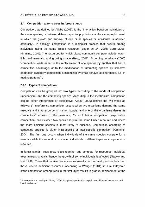
2.4� Competition among trees in forest stands ...................................................... 18�
2.4.1� Types of competition ............................................................................... 18�
TABLE OF CONTENTS ii
2.4.2� Spatial and non-spatial competition ........................................................ 19�
2.4.3� Measuring the degree of competition ...................................................... 20�
3� MATERIALS AND METHODS ........................................................................... 23�
3.1� Background .................................................................................................... 23�
3.2� Study area ..................................................................................................... 23�
3.2.1� Physical attributes ................................................................................... 25�
3.2.1.1� Climate ................................................................................................ 25�
3.2.1.2� Soil and topography ............................................................................ 26�
3.2.1.3� Vegetation cover ................................................................................. 27�
3.2.2� Population ............................................................................................... 29�
3.2.3� Land use patterns ................................................................................... 29�
3.2.4� Forest activities in the Umfakarin Natural Reserve Forest ...................... 31�
3.3� Data collection ............................................................................................... 32�
3.3.1� Reconnaissance survey .......................................................................... 32�
3.3.2� Pre-test samples ..................................................................................... 32�
3.3.3� Mensurational data ................................................................................. 33�
3.3.3.1� Single tree measurement .................................................................... 33�
3.3.3.2� Identifying the competitors .................................................................. 35�
3.3.3.3� Tree mapping ...................................................................................... 35�
3.3.4� Gum tapping and collection techniques .................................................. 37�
3.3.4.1� Background ......................................................................................... 37�
3.3.4.2� Selection and marking trees for tapping .............................................. 37�
3.3.4.3� Gum collection .................................................................................... 41�
3.4� Computational statistics of tree and stand values .......................................... 42�
3.4.1� Stand height curve .................................................................................. 43�
3.4.2� Volume functions .................................................................................... 44�
3.5� Quantification of competition indices using CroCom ...................................... 44�
3.6� Statistical analysis.......................................................................................... 47�
3.6.1� Test for normality .................................................................................... 47�
3.6.2� Simple linear correlation ......................................................................... 47�
3.6.3� Regression analysis ................................................................................ 48�
3.6.4� Post-Hoc tests in the analysis of variance (ANOVA) .............................. 53�
3.6.5� Regression tree ...................................................................................... 54�
3.7� Software ......................................................................................................... 55�
4� RESULTS .......................................................................................................... 57�
TABLE OF CONTENTS iii
4.1� Stand values .................................................................................................. 57�
4.1.1� Modelling height curves .......................................................................... 58�
4.1.2� Volume functions .................................................................................... 62�
4.1.3� Relationship between DBH and crown radius ......................................... 62�
4.2� Single tree values .......................................................................................... 65�
4.2.1� Competition indices (CI) and tree dimensions ........................................ 65�
4.2.1.1� Frequency distribution of CI-values ..................................................... 65�
4.2.1.2� Partial correlations .............................................................................. 65�
4.2.1.3� Selection of an appropriate competition index .................................... 68�
4.2.2� Production of gum talha from natural stands of A. seyal ......................... 71�
4.2.3� Factors affecting gum yield ..................................................................... 73�
4.2.3.1� Gum yield and tree size (DBH) ............................................................ 73�
4.2.3.2� Determining factors influencing gum yield using regression tree ........ 74�
4.2.3.3� Determining factors that influence gum yield using GLM .................... 75�
4.2.3.4� Determining factors affecting gum yield using logistic regression ....... 78�
5� DISCUSSION .................................................................................................... 80�
5.1� Stand characteristics ...................................................................................... 80�
5.1.1� Forest composition and structure ............................................................ 80�
5.1.2� Natural regeneration ............................................................................... 81�
5.1.3� Height-diameter relationship ................................................................... 81�
5.1.4� Single tree and stand volume functions .................................................. 83�
5.1.5� Crown radius-DBH relationship............................................................... 85�
5.2� Single tree values .......................................................................................... 85�
5.2.1� Competition among trees of A. seyal natural stands............................... 85�
5.2.2� Competition index in relation to tree dimensions .................................... 86�
5.2.3� Gum talha production ............................................................................. 87�
5.2.3.1� Factors affecting gum talha yield ......................................................... 88�
5.2.3.2� Gum yield in relation to tree diameter ................................................. 90�
5.2.3.3� Gum yield in relation to CI value ......................................................... 91�
5.2.4� Future prospects of gum talha ................................................................ 91�
SUMMARY AND ZUSAMMENFASSUNG ................................................................ 93�
SUMMARY ............................................................................................................... 93�
ZUSAMMENFASSUNG ............................................................................................ 94�
REFERENCES ......................................................................................................... 97�
APPENDICES ........................................................................................................ 108�

LIST OF FIGURES iv
LIST OF FIGURES
Figure 1.1 Distribution of Acacia seyal varieties in Africa, with respect to rainfall ....... 3�Figure 2.1 Sudan forest and other wooded land (OWL) areas 1990-2010 ................. 8�Figure 2.2 Gum belt in Africa including Sudan .......................................................... 11�Figure 2.3 Production trend of gum hashab and gum talha in Sudan ...................... 14�
Figure 2.4 Methods of selection the competitor trees ............................................... 22�Figure 3.1 Location of Umfakarin Natural Forest, South Kordofan, Sudan. .............. 24�Figure 3.2 Status of the Umfakarin Natural Forest in South Kordofan state forests . 25�Figure 3.3 Climatic diagram (1997-2006) for the Rashad Locality, South Kordofan . 27�Figure 3.4 Conditions of Umfakarin Natural Forest during rainy season, 2007/2008 27�Figure 3.5 Forest cover in Sudan and Kordofan ....................................................... 30�Figure 3.6 Regeneration of A. seyal in open areas in the Umfakarin Forest, 2007 ... 30�Figure 3.7 Forest activities in the Umfakarin Natural Forest Reserve, 2007/2008 .... 31�Figure 3.8 Different densities of A. seyal trees in the Umfakarin Forest, South Kordofan ................................................................................................................... 34�
Figure 3.9 Measuring pole used for marking the position of tree diameters ............. 34�Figure 3.10 Positions of neighborhood trees relative to the subject A. seyal tree ..... 36�Figure 3.11 Local tools used for tapping Acacia seyal for gum production ............... 38�Figure 3.12 Techniques for marking Acacia seyal trees for gum tapping ................. 39�Figure 3.13 Acacia seyal: gum tapping and collection techniques ............................ 40�Figure 3.14 Mean values of the dependant variable above and below the threshold of the explanatory variable............................................................................................ 55�Figure 4.1 DBH and height frequency distribution for A. seyal in the Umfakarin Forest ................................................................................................................................. 59�Figure 4.2 Observed data and the lines of best fit (evaluated height functions) for A.
seyal ......................................................................................................................... 60�Figure 4.3 Observed data and the line of best fit (Michailow height curve) of A. seyal ................................................................................................................................. 61�Figure 4.4 Volume function for A. seyal natural stands in different stand densities. . 63�Figure 4.5 Diameter at breast height (DBH) in relation to crown radius (CR) of A. seyal for different stand densities, Umfakarin Forest, South Kordofan, Sudan. ........ 64�Figure 4.6 Frequency distribution of the selected competition index values for Acacia seyal ......................................................................................................................... 66�Figure 4.7 Partial correlation between competition indices and A. seyal dimensions 67�Figure 4.8 Acacia seyal and the relationship between DBH and competition index (CI) values (CI_Hegyi_2) .......................................................................................... 70�Figure 4.9 Gum talha yield in relation to tree diameter for different stand densities . 73�Figure 4.10 Regression tree model for predicting yield of gum talha ........................ 75�Figure 4.11 Observed and predicted gum yield (g) of Acacia seyal at medium stratum ................................................................................................................................. 78�Figure 5.1 Michailow and parabolic height curves used for predicting height of A. seyal trees in Umfakarin natural forest, Sudan ......................................................... 83�Figure 5.2 Volume functions used for deriving volume of A. seyal in Sudan ............ 84�Figure 5.3 Regression tree model: DBH threshold and the mean gum talha yield (g)
................................................................................................................................. 89�
LIST OF TABLES v
LIST OF TABLES
Table 2.1 Gum producing trees, source and method of production in some African countries ................................................................................................................... 10�Table 3.1 Gum tapping and collection schedule ....................................................... 41�Table 3.2 Potential models used for evaluation of height-diameter relationship of A.
seyal ......................................................................................................................... 43�Table 3.3 Models used for CIs quantification in CROCOM Programme ................... 45�Table 3.4 Calculations for testing significant differences between slopes of kregression lines ........................................................................................................ 52�Table 4.1 Stand values of natural A. seyal in different stand densities ..................... 57�Table 4.2 Number per hectare of natural regeneration greater or less than 1.3 m height ........................................................................................................................ 58�Table 4.3 Models evaluated for the height curve of A. seyal natural stands in the Umfakarin Forest, South Kordofan, Sudan. .............................................................. 60�Table 4.4 Summary of estimated parameters of the Michailow function used for A
seyal height estimation in different strata, Umfakarin Forest, South Kordofan, Sudan. ................................................................................................................................. 62�Table 4.5 Summary of nonlinear regression parameters for volume as a function of DBH and height for A. seyal in different strata, Umfakarin Forest, South Kordofan, Sudan. ...................................................................................................................... 63�Table 4.6 Summary of nonlinear regression parameters for crown radius (CR, in m) in relation to DBH of A. seyal in different strata, Umfakarin Forest, South Kordofan, Sudan. ...................................................................................................................... 64�Table 4.7 Results of normality test of selected competition indices .......................... 65�Table 4.8 Relationship between CIs and tree dimensions in different A. seyal stand
densities ................................................................................................................... 69�Table 4.9 Average yield of gum talha and number of trees by different tapping treatments ................................................................................................................. 72�Table 4.10 Number of trees, total and average gum talha yield (g) per yield class and production (kg/ha) in different stand densities .......................................................... 72�Table 4.11 Post-hoc-test, following ANOVA, based on Scheffé test for testing the difference in gum talha yield ..................................................................................... 76�Table 4.12 Homogenous subset for average gum yield (g) based on Scheffé test... 77�Table 4.13 Classification table* of the logistic regression analysis of gum talha yield ................................................................................................................................. 79�Table 4.14 Results of logistic regression analysis (dependent variable: gum yield) . 79�

LIST OF APPENDICES vi
LIST OF APPENDICES
Appendix 1 Tree measurement and mapping form ................................................. 108�Appendix 2 Gum tapping and collection form ......................................................... 109�Appendix 3 Normality test of A. seyal tree dimensions ........................................... 110�Appendix 4 Results of regression tree analysis for predicting gum talha yield ....... 110�Appendix 5 Scheffe test (Post-hoc-test) after ANOVA for gum talha yield derived from natural A. seyal using different tapping tools in the Umfakarin Forest, South Kordofan, Sudan ..................................................................................................... 110�Appendix 6 GLM results: tests of between-subjects effects ................................... 111�

ACRONYMS AND ABBREVIATIONS vii
ACRONYMS AND ABBREVIATIONS
A. Acacia a.s.l. Above sea level AGB Above ground biomass AIC Akaike´s information Criterion
ANOVA Analysis of variance ARC Agricultural Research Corporation, Sudan BA Stand basal area (m²) per unit area BAL Basal area of the largest tree CART Classification and Regression Tree CD Crown diameter (m) CI Competition index cm Centimeter CPA Comprehensive Peace Agreement CPF Crown permeability factor
CR Crown radius (m) CrPA Crown projection area (m²) DBH Diameter at breast height (cm) FAO Food and Agricultural Organization of the United Nations FNC Forests National Corporation FRA Global Forest Resources Assessment GAC Gum Arabic Company Ltd. GLM General linear model IES Institute of Environmental Studies, University of Khartoum, Sudan IIED International Institute of Environment and Development
JECFA Joint Expert Committee on Food Additives LPG Liquefied petroleum gas m Meter MAI Mean annual increment MCR Mean crown radius for overstory trees mm Millimeter MSE Mean square error NAS National Academy of Science NCP National Congress Party, Sudan NFTA Nitrogen Fixing Tree Association NTFPs Non-timber forest products OWL Other wood land PI Periodic increment QMD Quadratic mean diameter RIZ Radius of influence zone ROI Radius of influence SPLA Sudanese People Liberation Army UNDP United Nations Development Program WHO World Health Organization

ACKNOWLEDGEMENTS viii
ACKNOWLEDGEMENTS
During the development of this thesis, there are many people from whom I have
received advice and encouragement I am greatly indebted to them.
I would like to express my deep gratitude and thanks to Prof. Dr. Heinz Röhle for his
continuous supervision and guidance during my PhD studies.
Thanks to Dr. Dorothea Gerold, Dr. Klaus Römisch and Prof. Dr. Uta Berger for their
comments and assistance in statistical analysis. Thanks also due to Juliane Vogt for
her effort to teach me R program and Janine Murphy, from Canada, for editing the
manuscript.
Without the support of many people the field work would not be possible. Among
them I would like especially to thank Mr. Mohamed Ahmed Ageed, Director, El
Abbassia forest Division, Mr. Hamed Elmanzoul, Inspector, Umfakarin forest and
Yahia Abutaba for their help and assistance.
I am also indebted to University of Kordofan for giving me this opportunity to study in
Germany and to the Ministry of Higher Education and Scientific Research, Sudan for
the scholarship.
Last but not least, I would like to thank all my colleagues at Institute of Forest Growth
and Forest Computer Sciences, TU-Dresden for their valuable comments and help.
Special thanks to Ms. Skibbe for translating the summary and theses to German
language. I would like also to thanks the Sudanese group in Dresden for their lovely
companion. Grateful thanks are also due to my colleagues (Mr. Elsheikh A/Kareem,
Dr. Awad Abdalla and Mr. Ismael Ahmed) for following up some issues in Sudan
relevant to my study. Special thanks are due to my wife and my kids for their patient
and encouraging me during their stay in Germany.

CHAPTER 1: INTRODUCTION 1
1 INTRODUCTION
1.1 Background
Acacia seyal Del. is a typical tree in the African semi zones. It is a small to medium-
sized tree that reaches a height of 12-17 m (Hall and McAllan, 1993; McAllan, 1993;
von Maydell, 1990; National Academy of Sciences, NAS, 1980), has a stem diameter
of 30 cm (Mustafa, 1997), or 60 cm under favourable conditions, and develops a
characteristic umbrella-shaped crown (von Maydell, 1990). Acacia seyal usually
reaches 9-10 m in height at maturity (Nitrogen Fixing Tree Association, NFTA, 1994).
Several authors provide a valuable description of Acacia seyal (see for example;
Elamin, 1990; Hall and McAllan, 1993; McAllan, 1993; Mustafa, 1997; von Maydell,
1990; NAS, 1980).
Like other acacias, A. seyal is widely distributed in the African savannas (Booth and
Wickens, 1988; McAllan, 1993), often dominates the vegetation community and in
some areas forms pure stands (McAllan, 1993; Wickens et al., 1995). It is considered
one of the most common trees on clay plains that flood during the rainy season
(McAllan, 1993).
The species is an important source of fuel wood, building poles, forage, commercial
gums, and tannins (ELamin, 1990; Mustafa, 1997; von Maydell, 1990; NAS, 1979,
1980; Wickens et al., 1995) and is a source of nectar for honeybees (Booth and
Wickens, 1988). A. seyal produces gum which though of inferior quality in
comparison to that of Acacia senegal, is traded in Sudan under the name ´´gum
talha´´ and makes up to 10 percent of the annual exported gum Arabic (Barbier et al.,
1990; McAllan, 1993; NFTA, 1994). Unlike gum from A. senegal, gum talha is not
recognized as an acceptable food additive (Hall and McAllan, 1993).
Additionally, A. seyal serves valuable ecological functions such as reducing soil
erosion and acting as a defence line for desert encroachment in many parts of the
Sudan, as is the case for the selected location for the present study, the Umfakarin
forest reserve. Like other Leguminous, A. seyal is a nitrogen fixing tree which can be
integrated into an agro-forestry system to enhance the growth of agricultural crops.

CHAPTER 1: INTRODUCTION 2
The species requires annual rainfalls of 250-1000 mm and it can withstand
inundation better than other acacias (von Maydell, 1990; NAS, 1980). The species
thrives in most soil types, even in heavy clay and stony soils found on the plains
(McAllan, 1993; NAS, 1980). It prefers temperatures between 15-35 ºC (Vogt, 1995).
It often grows with other tree species, such as Acacia sieberana, Anogeissus
leiocarpus, Balanites aegyptiaca, Faidherbia albida and Ziziphus mauritiana
(McAllan, 1993).
In general, there are two main varieties of A. seyal; variety seyal and variety fistula.
Variety seyal is found in both western and eastern Africa and also on the Arabian
Peninsula, while variety fistula is found in the eastern parts of Africa (McAllan, 1993).
NAS (1980) and NFTA (1994) indicate that variety seyal is native to northern-tropical
Africa and Egypt. The two varieties can be easily distinguished; variety seyal has a
greenish-yellow to reddish-brown bark, while variety fistula has white to greenish-
yellow bark (McAllan, 1993). Figure 1.1 shows the distribution of A. seyal varieties,
with respect to rainfall.
In Sudan, the two varieties occur naturally in the low rainfall savannah zone and
extend from Gadarif, Blue Nile, and White Nile to clay plains around Nuba Mountains
and the Darfur Region (El Amin, 1990; Mustafa, 1997; Sahni, 1968). The species is
distributed throughout its natural range, and is usually associated with Balanites
aegyptiaca in the Acacia seyal-Balanites woodland area. In such formation, A. seyal
is the dominant species, forming pure dense stands in many areas. According to
Mustafa (1997), this formation begins to emerge with an increase in the annual
rainfall to accumulations of more than 500 mm.
In the savanna region of Sudan, A. seyal has been subjected to large-scale clearing
for mechanized agriculture (Mustafa, 1997; Vink, 1990; Wickens et al., 1995)
associated with firewood and charcoal production to meet energy requirements.
Besides clearance for mechanized farming and wood fuel, other factors such as
grazing, deliberate and undeliberate fires also have a significant negative impact, not
only on natural stands of A. seyal but also on natural forests in Sudan.

CHAPTER 1: INTRODUCTION 3
(Source: Hall and McAllan, 1993; McAllan, 1993)
Figure 1.1 Distribution of Acacia seyal varieties in Africa, with respect to rainfall
Var. seyal Var. fistula

CHAPTER 1: INTRODUCTION 4
1.2 Problem statement
Much of the pressure on Sudan's forests is caused by the exploitation of wood
resources for mechanized farming and fuel-wood. The dependence of more than 80
percent of Sudan’s rural population on the wood biomass for their daily energy needs
has accelerated the depletion of natural forest resources, as wood biomass is the
most dominant and accessible source of energy. About 200,000 hectares of natural
woodlands and forests are annually replaced and claimed by the agriculture (FAO,
2005) associated with the production of firewood and charcoal. As a result of such
activities, for example mechanized farming and the extraction of wood fuel, natural
forest areas have been fragmented and their ecological functions have notably
decreased. Additionally, wood volume extracted from natural forests has also
decreased. A. seyal natural stands provide a typical example to this practice, where
vast areas are annually replaced for the above mentioned purposes.
A. seyal grows naturally in the clay plains of central and eastern Sudan and has
extensively managed for firewood and charcoal production in order to meet energy
requirements. The species forms either pure stands of different densities (dense,
medium to poor) or mixed stands associated with other tree species.
Forest management in Sudan mainly focuses on wood production, for either fuel
wood or sawn timber, in plantations and/or natural forests. However, non-timber
forest products (NTFPs) extracted from natural forests and/or plantations, such as
gum, are also very important and often have significant contribution to rural and
national economies of many African countries (Ballal, 2002; Chikamai et al., 2009;
Seif el Din and Zarroug, 1998). For example, in the Liban district of Ethiopia,
Lemenih et al. (2003) indicated that gum production activities contribute to about 33
percent of the annual household subsistence, ranking second after livestock in the
overall household livelihood. Included in these NTFPs is gum talha, the natural
product of A. seyal.
The natural gum exudate (gum talha) is obtained from stems and branches of A.
seyal trees. In some areas, such as Kordofan and Darfur regions, gum talha is
collected by local people and sold in the market; separate from gum hashab (gum
from A. senegal). In some regions of Ethiopia, gums obtained from A. senegal and A.
CHAPTER 1: INTRODUCTION 5
seyal, are also traded separately (Lemenih et al., 2003). Although, the species is
reported to produce a significant amount of gum talha, little information is known
about the potential of the species to produce gum.
Studies on the potentiality of A. seyal to produce gum under different stand densities
and its response to tapping techniques, giving consideration to the amount of gum
yielded by tree per season, are limited. Trees of A. seyal usually grow under different
stand densities. Thinning practices often take place to reduce competition among
trees, mainly to enhance tree growth for wood production. Such practices are rarely
conducted for the promotion of gum talha production. Information regarding the effect
of tree competition on gum talha production is limited.
1.3 Objectives of the study
Based on the problems outlined above, the general objective of this study is to
manage the natural stands of A. seyal for production of gum talha.
Specific objectives
In order to realize the general goal of the current study, the following specific
objectives are formulated:
• to determine the standing volume of natural A. seyal growing in different stand
densities;
• to study the competition among trees of A. seyal in natural stands;
• to examine the effect of tapping techniques (tools) and time of tapping on gum
talha productivity; and
• to develop models to be used for the prediction of gum talha yields.
1.4 Hypotheses of the study The following hypotheses are proposed:
• There are high differences in gum talha yield due to tree competition.
• Yield of gum talha is affected by tapping techniques and time of tapping.
• Tree dimensions, such as the diameter at breast height (DBH), has an impact
on gum talha yield.

CHAPTER 1: INTRODUCTION 6
1.5 Organization of the study
The study consists of five main chapters. The first chapter provides the general
background on the natural stands of A. seyal, including its distribution and uses.
Here, the problem statement, objectives and hypotheses of the study are also
highlighted. A literature review is highlighted in the second chapter. This chapter also
describes in general natural forest resources in Sudan, with special reference to the
management of natural A. seyal stands. Furthermore, gum producing trees and the
production of gum talha from natural stands of A. seyal and the factors that affect its
production are also presented in this chapter. Chapter two also focuses on the
competition among A. seyal trees of different stand densities. Physical attributes of
the study area, beside its population, land use patterns and forest activities, are
addressed in the third chapter. The methods used for data collection and analysis are
explained in the same chapter. Results and discussion are highlighted in chapter four
and five, respectively. A summary of the thesis, zusammenfassung (summary in
German), references and appendices are provided at end of the thesis. Part of the
results of this thesis was presented in international conferences1 and published in
scientific journals.
1 Publications:
Mohammed, M. H. and Röhle, H. (2009). Effect of tree density and tapping techniques on the productivity of gum talha from Acacia seyal in South Kordofan, Sudan. International Conference on Research on Food Security, Natural Resource Management and Rural Development, Oct. 6-8, 2009, Hamburg. ISBN: 978-3-9801686-7-0 (Book of abstracts p 402). URL: http://www.tropentag.de/2009/abstracts/full/93.pdf.
Mohammed, M. H. and Röhle, H. (2010). Gum talha from Acacia seyal Del. variety seyal in South Kordofan, Sudan. Research Journal of Forestry, accepted on December 8, 2010.
Mohammed, M. H. and Röhle, H. (2010). Studying the competition in natural stands of Acacia seyalDel. variety seyal. International Conference Forestry: Bridge to the Future. University of Forestry, Sofia, May 13-15, 2010, Bulgaria. Book of abstracts p 93; ISBN: 978-954-332-072-1. Paper submitted on May 13, 2010 to journal “Forest Ideas” issued by the University of Forestry in Sofia.

CHAPTER 2: SCIENTIFIC BACKGROUND 7
2 SCIENTIFIC BACKGROUND
2.1 Natural forest resources in Sudan
Various forest inventories were created in order to study the extent and the
composition of forest resources in Sudan (Dawelbait et al., 2006). However, the
majority of previous forest inventories were either partially conducted (not covering
the whole country) or are incomplete (Dawelbait et al., 2006; Forests National
Corporation, FNC, 2007). Based on these inventories, the total area of forest in
Sudan is estimated to cover about 28 percent of the country’s total land (250.6 million
hectares), of which only 4.8 per cent was reserved2 in 2007 (Forest Resources
Assessment, FRA, 2010). Nevertheless, the Comprehensive National Strategy (CNS
1992-2002), a government formulated and enacted policy, called for the allocation of
25% (59.4 million hectares) of the country’s total area for forest reserves (FNC,
2007). This estimate does not include other wooded lands3 (OWL), areas which are
estimated, according to the recent estimates of Global Forest Resources
Assessment in 2010, to cover about 20 percent of the country’s total area. Estimates
of forest and other wooded land areas over time are provided in Figure 2.1.
According to these numbers, forest area is seemingly constant after 2000, but the
changes in OWL areas may be attributed to the conversion of OWL into forests
(FRA, 2010).
The World Bank (1986, cited in Mustafa, 1997) approximated that the average
growing stock for natural forests in the Sudanese dry lands was about 24 m³/ha.
However, recently the total growing stock of forest and OWL was estimated to be 5.5
m³/ha and the above ground biomass (AGB) is believed to be about 13 metric tons
oven-dry weight (FRA, 2010). The share of biomass in total energy consumption was
projected to account for from 71 to more than 82 percent of the total energy
consumed in the country (FNC, 2007; Salih, 1994). After the commencement of oil
production, the use of biomass energy alternatives, for example liquefied petroleum
2 According to FRA’s (2010) definition, forest reserves are all forest areas registered in the government
gazette as Forest National Corporation assets. In these reserves, cutting trees is concentrated and replanting is made immediately after removal.
3 Other wooded land is defined, according to FRA (2010), as land not classified as a “Forest”, which
spans more than 0.5 hectares, has trees higher than 5 meters, and a canopy cover of 5-10 percent, or trees able to reach these thresholds in situ. OWL may also be a combination of shrubs, bushes and trees above 10 percent. It does not include land that is predominantly used for agricultural or urban
land.

CHAPTER 2: SCIENTIFIC BACKGROUND 8
gas LPG, kerosene, etc, will have a positive impact on reducing pressure on natural
forests (FNC, 2007).
Source: (FRA, 2010)
Figure 2.1 Sudan forest and other wooded land (OWL) areas 1990-2010
2.2 Production of acacia gum
2.2.1 Gum producing acacia tree species
The genus acacia, family mimosaceae, is widely distributed in the tropical and
subtropical regions of the world, most commonly in Africa and Australia in addition to
the Asia-Pacific region and the Americas (Orchard and Wilson, 2001). Gum acacia is
a natural gum derived from acacia trees. Various acacia tree species, in several
semi-arid African countries, are known to produce gum (Chikamai, 1999).
2.2.1.1 Gum from acacia natural stands
Natural acacia woodlands occupy large areas of the African savannah. According to
Chikamai (1999) most acacia species produce gum based on natural exudation in
natural stands and only four of them produce gum based on tapping, including A.
senegal in nine African countries including Sudan, A. laeta in Chad and Mali, A.
ehrenbergiana in Senegal and A. Karroo in Zimbabwe. Table 2.1 provides a
summary of some acacia species (gum-producing trees), and the source and method
of gum production in selected African countries.
�
�����
�����
�����
�����
�����
�����
����
����
�����
���� ���� ���� ����
����
�������������� �
� ����
���

CHAPTER 2: SCIENTIFIC BACKGROUND 9
2.2.1.2 Gum from acacia plantations
Brown (2000) stated that “acacias are planted mainly in Africa, Indonesia and on the
Indian subcontinent”. In some African countries, Burkina Faso, Ethiopia, Mali,
Mauritania, Niger, Senegal and Sudan, acacia plantations are established for the
production of gum Arabic mainly from the A. senegal species (Brown, 2000;
Chikamai, 1999). Indonesian acacia plantations, i.e. A. mangium, are mainly
established to supply wood material for pulp and paper industries (Aruan, 2004).
Other countries establish acacia plantations for different purposes such as soil and
water protection, recreational purposes, as fuel-wood, and for sawn timber (Brown,
2000; Elsiddig, 2003a; Orchard and Wilson, 2001).
Recent studies carried out by Ballal et al. (2005b) in Sudan investigated the gum
yield variations in natural stands and plantations of A. senegal under different
management regimes. In general, the average gum yield from A. senegal in Sudan is
about 250 g/tree/season (IIED and IES, 1990). Previous estimates of gum Arabic
yield from the same species were found to range from 100-200 g/tree (FAO, 1978).
According to Ballal (2002), the type of stand was factored into the above estimates.
In this context, he estimated the yield of gum hashab (gum derived from A. senegal)
in plantations and natural stands. His estimates ranged from 40.5-87 and 33.0-47.7
kg/ha in plantations and natural stands, respectively.
2.2.2 Gum belt
Geographically (Figure 2.2), the gum belt occurs as a broad band that ranges from
Mauritania, Senegal and Mali in the west, through Burkina Faso, northern Benin,
Niger, and northern parts of Nigeria, Cameroon and Chad and from the northern
Central African Republic to Sudan, Eritrea, Ethiopia and Somalia in the Horn of Africa
(Ahmed, 2006). According to the International Institute for Environment and
Development IIED and the Institute of Environmental Studies IES (IIED and IES,
1990), the Sudanese gum Arabic belt marks the area of Central Sudan, extending
between 10 and 14°N and accounts for around one fif th of Sudan’s total area,
covering an area where low rainfall interacts with sandy and clay soils. The belt acts
as an important area as it provides vital economic activities for rural communities.
Rural people within the Sudanese gum belt derive their income from several land-use
activities, including agriculture, grazing, and forest exploitation such as the collection
of forest products including gum Arabic (Sulieman, 2008). Within this region, A.

CHAPTER 2: SCIENTIFIC BACKGROUND 10
senegal is the only tree species which is planted and protected by farmers
(Mohamed, 2006).
Table 2.1 Gum producing trees, source and method of production in some African countries Production source Production method
Botanical source Plantations Natural stands Tapping Natural exudate
Burkina Faso A. senegal A. laeta A. seyal A. gourmaensis
A. duggeoni A. raddiana
** ** ** ** **
** **
** ** ** **
** **
Chad A. senegal var. senegal A. laeta A. seyal A. polycantha
**
** ** **
**
**
**
** ** **
Ethiopia A. senegal var. senegal A. senegal var. kerensis
A. seyal var. seyal A. seyal var. fistula A. polyacanthat A. drepanolobium
** **
**
** ** ** **
** **
**
** ** ** **
Ghana A. sieberana A. polyacantha
** **
** **
Kenya A. senegal var. kerensis A. paoli
**
**
**
**
Mali A. senegal
A. laeta A. seyal A. polycantha A. raddiana
**
**
**
** ** ** **
**
**
**
** ** ** **
Mauritania A. senegal A. laeta A. seyal
A. macrostachya
** ** ** **
**
** ** ** **
**
Niger A. senegal A. seyal A. raddiana
A. tortilis A. polyacanthat
** ** ** **
** **
** ** **
** **
Nigeria A. senegal var.
senegal A. seyal var. seyal A. nilotica
**
** **
** **
** **
Senegal A. senegal
A. ehrenbergiana A. laeta A. macrostachya A. macrothyrsa A. nilitica A. polycanthat A. sieberana A. tortilis
** **
** ** ** ** ** ** ** **
**
**
**
** ** ** ** ** ** ** **
Sudan A. senegal var. senegal A. seyal var. seyal
** **
**
** *
**
Zimbabwe A. karroo ** ** **
**: indicates gum production source and method of production. Source: (Chikamai, 1999)

CHAPTER 2: SCIENTIFIC BACKGROUND 11
Source: (Elmqvist et al., 2005)
Figure 2.2 Gum belt in Africa including Sudan
2.2.3 Gum Arabic production in Sudan
Gum Arabic4 producing trees grow in most African countries, especially in Sub-
Saharan Africa; nevertheless, most of the world's gum Arabic supply comes from
Sudan (Ahmed, 2006; Wickens et al., 1995). In Sudan, several acacia species
produce gum of different quantities and qualities. However, only gum Hashab (gum
from Acacia senegal) is permitted for the food trade and the remaining types are
used for industrial purposes (Wickens et al., 1995).
Gum Arabic is an important natural product of Acacia senegal (L.) Willd. and Acacia
seyal Del. trees (IIED and IES, 1990). In Sudan, gum Arabic is obtained by tapping
A. senegal trees in natural stands and/or plantations (Abdelnour 1999; Ballal et al.
2005a). However, gum from A. seyal (talha) is mostly obtained from natural stands
and through natural exudation (Abdelnour, 1999; Seif el Din and Zarroug, 1998).
Sudan leads the world in the production and exportation of gum Arabic and accounts
4 According to the Joint Expert Committee on Food Additives (Joint FAO/WHO Expert Committee on
Food Additives, JECFA, 1997), gum Arabic is defined as the dried exudate obtained from the stems
and branches of Acacia senegal (L) or closely related species like A. seyal.
CHAPTER 2: SCIENTIFIC BACKGROUND 12
for about 80 percent of the world’s gum Arabic production (Abdelnour, 1999;
Abdelnour and Osman, 1999; FNC, 2007; Tadesse et al., 2007). At the end of the
1990s, it contributed 70–90% of the world’s production (Elmqvist et al., 2005).
However, recently gum production in Sudan has declined and yields also vary
increasingly from year to year due to several factors, such as deforestation (Rahim,
2006) and price policies (Elmqvist et al., 2005). The product is one of the main
agricultural export commodities produced in traditional rain-fed agriculture
(Abdelnour, 1999; IIED and IES, 1990).
2.2.3.1 Gum Arabic production methods in Sudan
Gum Arabic, particularly gum from A. senegal trees, is collected by tapping A.
senegal trees (local name: hashab), whereas natural exudation is collected from
other acacia species. Gum Arabic production in Sudan is practiced using two main
production systems, hashab owners and hashab renters. Many studies describe the
two production systems of gum Arabic in Sudan (Ahmed, 2006; IIED and IES, 1990).
Most of the gum is produced by smallholders on individual farms where the trees
grow naturally (Elmqvist et al., 2005). Tapping, by making small incisions into the tree
bark, begins in the hot and dry season when trees start to shed their leaves
(Abdelnour, 1999; Ahmed, 2006). Trees that exceed 4 years in age are usually ready
for tapping (IIED and IES, 1990). Traditional axes have been used for tapping A.
senegal trees. Recently, a recommended tool (locally: sonki) that was designed and
released by the Agricultural Research Centre (ARC), Sudan, has also been used for
tree tapping. First gum exudatation is collected in 4-6 weeks after tapping and the
subsequent collections (up to seven) are done every 15 days (Abdelnour, 1999; IIED
and IES, 1990).
Several scholars have assessed the variations in gum arabic production in Sudan
(see for example: Ballal et al., 2005b; IIED and IES, 1990). Studies by the IIED and
IES (1990), indicated that there are pronounced variations in A. senegal stands both
in clay and sandy areas, in terms of stand area, condition, stand density, production
age, method of tapping, accessibility to producers, and the supply of inputs.
In other countries, such as Nigeria and Ethiopa, gum arabic production per unit area
also varies according to stand type. In the Zamfara State, Nigeria, Unanaonwi (2009)
studied the gum Arabic yield in plantations and natural stands. He showed that the
CHAPTER 2: SCIENTIFIC BACKGROUND 13
average gum yield per tree was estimated to be 85.0 and 87.7g, corresponding to
53.1 and 18.6kg/ha, respectively, for plantations where stand density is 625 trees per
hectare and natural forests where there are 212 stems per hectare. In Liban,
Ethiopia, annual production per hectare ranged between 66.6 to 202.6 kg (Lemenih
et al., 2003). Lemenih et al. used results based on households interviews to estimate
gum production per unit area from different acacia woodlands.
2.2.3.2 Gum talha the natural exudate from Acacia seyal
Gum talha is a natural exudate obtained from both the stem and branches of A.
seyal. According to the Joint FAO/WHO Expert Committee on Food Additives
(JECFA, 1997) specification, gum talha is included in the term “gum Arabic” defined
as the dried exudation obtained from the stems and branches of A. senegal (L.) or
closely related species such as A. seyal. However, in Sudan, the gum from A.
senegal and A. seyal are separated in both national statistics and trade (FAO, 1995).
Unlike A. senegal, A. seyal in Sudan has not been cultivated for gum production.
Nevertheless, the species is reported to produce significant amount of gum and has
many traditional and industrial uses, which are generally friable and inferior to that of
A. senegal (Anderson et al., 1984; FAO 1995; Hall and McAllan 1993; McAllan 1993).
2.2.3.2.1 Production of gum talha in Sudan
Despite the extensive use of A. seyal for firewood and charcoal, the species
produces gum talha and constitutes to about 10 percent of Sudan’s total gum
production, of which more than 50 percent comes from Kordofan region (Gum Arabic
Company, GAC, 2008). This amount of gum production is collected only from natural
exudates by local people in western Sudan (Fadl and Gebauer, 2004). Macrae and
Merlin (2000) indicated that “the potential production of talha gum in Sudan is very
large–estimated at least twice the amount of hashab hard gum”. Furthermore, they
noted that this type of gum is not promoted by the Sudanese government, and thus
remains attached to its reputation and market dominance in the hashab sector of the
market.
Figure 2.3 depicts the general trend of gum Arabic in Sudan. Generally, the annual
production of hashab gum fluctuates due to climatic variations (IIED and IES, 1990).
In the case of gum talha, production potential estimates indicate that the mean
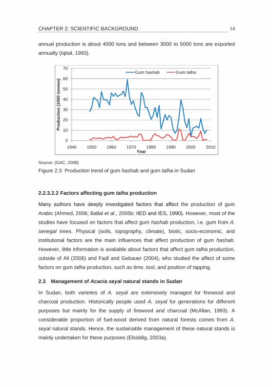
CHAPTER 2: SCIENTIFIC BACKGROUND 14
annual production is about 4000 tons and between 3000 to 5000 tons are exported
annually (Iqbal, 1993).
Source: (GAC, 2008)
Figure 2.3 Production trend of gum hashab and gum talha in Sudan
2.2.3.2.2 Factors affecting gum talha production
Many authors have deeply investigated factors that affect the production of gum
Arabic (Ahmed, 2006; Ballal et al., 2005b; IIED and IES, 1990). However, most of the
studies have focused on factors that affect gum hashab production, i.e. gum from A.
senegal trees. Physical (soils, topography, climate), biotic, socio-economic, and
institutional factors are the main influences that affect production of gum hashab.
However, little information is available about factors that affect gum talha production,
outside of Ali (2006) and Fadl and Gebauer (2004), who studied the affect of some
factors on gum talha production, such as time, tool, and position of tapping.
2.3 Management of Acacia seyal natural stands in Sudan
In Sudan, both varieties of A. seyal are extensively managed for firewood and
charcoal production. Historically people used A. seyal for generations for different
purposes but mainly for the supply of firewood and charcoal (McAllan, 1993). A
considerable proportion of fuel-wood derived from natural forests comes from A.
seyal natural stands. Hence, the sustainable management of these natural stands is
mainly undertaken for these purposes (Elsiddig, 2003a).
0
10
20
30
40
50
60
70
1940 1950 1960 1970 1980 1990 2000 2010
Pro
du
ctio
n (
1000
to
nn
es)
Year
Gum hashab Gum talha

CHAPTER 2: SCIENTIFIC BACKGROUND 15
Generally, in semi-arid savannas the growth rate of A. seyal is low; however, early
growth rates can be quite fast, trees can reach up to 1 meter in 3 months on
favorable sites (McAllan, 1993). As indicated by Mustafa (1997), A. seyal trees can
reach its reproductive stage rapidly, within 5 years in a natural stand, unless the
growth is retarded by local events such as intensive browsing or fire. The periodic
increment (PI) of the diameter at breast height and volume, respectively, does not
exceed 1.3 cm and 5 m³/ha in 3 years (Vink, 1990a). In Sudan, the growth and yield
of A. seyal vary according to region. For example, the mean annual increment (MAI),
of A. seyal, in Garri forest, Blue Nile, ranged between 1.6-2.4 m³/ha/year during
1963-1966, where recorded annual rainfall was 657 to 718 mm. However, the MAI
ranged between 1-1.5 m³/ha in the Rawashda forest in eastern Sudan (Vink, 1990a),
where annual rainfall ranges between 450-500 mm. Trees managed on a 10-15 year
rotation yield 10-35 m³/ha of fuel-wood per year (Orwa et al., 2009).
2.3.1 Volume and height functions for Acacia seyal
To estimate volume in forest stands, adequate and reliable allometric functions are
needed to be established (Bjarnadottir et al., 2007). These functions (formulas 1 and
2) mathematically describe the relationship between the tree volume and diameter at
breast height (DBH) and/or the height of the tree (Bjarnadottir et al., 2007; Pretzsch,
2009; West, 2004).
As the management of A. seyal in Sudan is mainly undertaken for fuelwood, most of
the studies were conducted as part of the project “fuelwood development for energy
in Sudan”. Volume and height functions have been developed, respectively, for
predicting volume and the height of A. seyal in natural stands (Elsiddig, 2003b).
)(dfv = ……………………………………………………….......................................... (1)
),( hdfv = …………………………………………………………………………...….….. ( 2)
This means, volume ( v ) is a function ( f ) of diameter ( d ) when using only ( d ) such
as in formula (1) or a function of d and height ( h ) when using both d and h as
predictors (formula 2).
The height function (3) is another allometric function that describes the relationship
between tree height and DBH (Kramer und Akça, 2008; West, 2004). It is also used
to predict tree height using DBH as a predictor.
)(dfh = …………………………………………………………………………………… (3)

CHAPTER 2: SCIENTIFIC BACKGROUND 16
The stand height curve can be used to provide information about the development
and growth stages of the stand; for example it can help determine whether it is a
young or old stand. It also provides information about the competitive situation of the
trees in the stand.
2.3.2 Silvicultural characteristics of Acacia seyal
The silvicultural system is a set of rules applied to a forest stand in order to ensure its
renewal (Bollefontaine et al., 2000). There are three basic silvicultural systems that
may be identified for natural forests in dry tropical zones; the coppice system, the
high forest system, and the coppice with standards system. The coppice system is
made up of stump and/or root sprouts, originating from “rejuvenation” cuttings, which
constitute a vegetative reproduction system. The “high forest” is a stand made up of
trees directly grown from seed on site. The “coppice with standards” is a mixed
system designed to perpetuate stands with trees of which some have originated from
seeds and others are derived from vegetative regeneration (Bollefontaine et al.,
2000).
2.3.2.1 Direct seeding
Many direct seeding trials have been carried out in the dry tropical zones, and their
success depends on several factors, such as seed quality, weed competition and
anthropogenic disturbance (Bollefontaine et al., 2000). In general, propagation of A.
seyal occurs via self-seeding and root suckers (Orwa et al., 2009). Nevertheless,
seedlings can be raised in the tree nursery from seed or cuttings (McAllan, 1993). A.
seyal can be established by direct seeding if there is reliable rainfall and adequate
protection for the seedlings (Hall and McAllan, 1993; McAllan, 1993; Mustafa, 1997).
Seed pretreatment, for example scarification, sulphuric acid treatment (Orwa et al.,
2009), or soaking in hot water for 30 minutes (Hall and McAllan, 1993; McAllan,
1993), is important to accelerate seed germination but not essential. Management
through coppicing is also possible and may help regenerate and manage species
with good coppicing ability (Mustafa, 1997).
2.3.2.2 Natural regeneration of Acacia seyal
Regeneration is an important aspect for the development and management of forest
stands. Therefore, the success of natural forest management depends on the

CHAPTER 2: SCIENTIFIC BACKGROUND 17
success of natural regeneration which is influenced by many factors. The most
important of which are soil seed bank (Du et al., 2007), gap size (Myers et al., 2000)
and biophysical and soil factors, in addition to other disturbance factors such as the
presence of herbivores and fires. Mustafa (1997) investigated some of these factors
in his study on A. seyal regeneration in the dryland region of the Sudan clay plain. In
order to maintain the ecological and other functions of the forest, it is necessary to
gather information about regeneration. Natural regeneration starts when gaps occur.
However, Mustafa (1997) illustrated that A. seyal seedlings were recruited from
naturally dispersed seed regardless of the available gap size between the individual
tree crowns.
2.3.2.3 Thinning
Savannah acacias’ natural mortality is normally caused either due to competition or
other disturbing factors such as fires, browsing, and droughts (Bukhari, 1998; Smith
and Goodman, 1986). Like other savanna acacias, A. seyal responds to spacing and
thinning regimes. According to NFTA (1994) A. seyal, for the production of poles and
firewood in Sudan, has an assumed initial stock of 1000 stems per hectare, however
regular thinning after 10 and 14 years can reduce stocking to 675 and 450 stems/ha,
respectively. Employing a 4 m grid for spacing is suitable for sorghum and sesame
intercropping (McAllan, 1993; NFTA, 1994).
Forest authorities in Sudan direct the commercial logging of mostly A. nilotica in the
reserved riverine forests and A. seyal for firewood and charcoal to supply the cities,
mostly via clearing A. seyal and other acacias from areas allocated for agriculture
(Gorashi, 2001).
2.3.2.4 Pruning
Evaluations of the response to pruning all branches of A. seyal trees, for example
pollarding and lopping, indicates a limited recovery capacity in mature trees and may
lead to mortality (Bollefontaine et al., 2000; Orwa et al., 2009). In the dry season in
western Sudan, the cattle owners formerly lopped the branches or the entire crown
for their cattle in times of fodder scarcity (McAllan, 1993; Orwa et al., 2009).
CHAPTER 2: SCIENTIFIC BACKGROUND 18
2.4 Competition among trees in forest stands
Competition, as defined by Allaby (2006), is the “interaction between individuals of
the same species, or between different species populations at the same trophic level,
in which the growth and survival of one or all species or individuals is affected
adversely”. In ecology, competition is a biological process that occurs among
individuals using the same limited resource (Begon et al., 2006; Berg, 2008;
Kimmins, 2004). The resources for which plants commonly compete include water,
light, soil minerals, and growing space (Berg, 2008). According to Allaby (2006)
“competition leads either to the replacement of one species by another that has a
competitive advantage, or to the modification of interacting species by selective
adaptation (whereby competition is minimized by small behavioral differences, e.g. in
feeding patterns)”.
2.4.1 Types of competition
Competition can be grouped into two types, according to the mode of competition
(mechanism) and the competing species. According to the mechanism, competition
can be either interference or exploitative. Allaby (2006) defines the two types as
follows: 1) interference competition occurs when two organisms demand the same
resource and that resource is in short supply, and one of the organisms denies its
competitors5 access to the resource; 2) exploitation competition (exploitative
competition) occurs when two species require the same limited resource and where
the more efficient species is most likely to succeed. Competition according to
competing species is either intra-specific or inter-specific competition (Kimmins,
2004). The first one occurs when individuals of the same species compete for a
resource while the second occurs when individuals of different species compete for a
resource.
In forest stands, trees grow close together and compete for resources. Individual
trees interact spatially; hence the growth of some individuals is affected (Gadow and
Hui, 1999). Trees that receive few resources usually perform and produce less than
those receive sufficient resources. According to Wenger (1984), in a multi-layered
stand competition among trees in the first layer results in gradual replacement of the
5 A competitor according to Allaby (2006) is a plant species that exploits conditions of low stress and
low disturbance.

CHAPTER 2: SCIENTIFIC BACKGROUND 19
intolerant trees and that leads to succession. Schwinning and Weiner (1998) in their
study about the mechanisms of competition among plants stated that “when plants
are competing, larger individuals often obtain a disproportionate share of the
contested resources and suppress the growth of their smaller neighbors”. They
further defined the mode of competition among plants according to their sizes into
five categories. These include:
• complete size symmetric competition where resource uptake among
competitors is independent of their relative sizes;
• partial size symmetry competition when the uptake of contested resources
increases with plant size, but less than proportionally;
• perfect size symmetry where the uptake of the contested resources is
proportional to size (equal uptake per unit size);
• partial size asymmetry where the uptake of contested resources increases
with plant size, and larger plants receive a disproportionate share; and
• completely size-asymmetric competition, where the largest plants obtain all
the contested resources.
Schwinning and Weiner (1998) also identified other types of competition such as
“one-sided competition” or “dominance and suppression”, referring to the mode of
competition that exists when larger plants obtain all the contested resource. In this
case, the available resources assigned for the smaller plants decrease and, under
severe competition, this leads to natural mortality.
2.4.2 Spatial and non-spatial competition
As noted by Hasenauer (2006), “the basic principle for most of the competition
processes assumes a certain minimum distance between neighboring trees before
competition occurs”. Based on this principle, competition can be distance-dependent
or distance-independent (Alder, 1995; Hasenauer, 2006; Vanclay, 1994; Wimberly
and Bare, 1996). The distance-dependent or spatial competition is based on the
measurements of tree coordinates or locations (Biging and Dobbertin, 1992; Hegyi,
1974; Münder and Schröder, 2001; Pretzsch 1995; Pretzsch, 2009) in addition to
stem and crown size (Pretzsch, 2009). Distance-independent or non-spatial
competition is based on the measurements of stand density (Nagel, 1999; Pretzsch,
2009; Wykoff et al., 1982). Position-dependent and position-independent are also

CHAPTER 2: SCIENTIFIC BACKGROUND 20
termed by Pretzsch (2009) referring to distance-dependent and distance-
independent, respectively. Furthermore, he provides a valuable description of
different approaches for measuring distance-dependent and distance-independent
competition indices.
2.4.3 Measuring the degree of competition
Measuring the degree of competition is an important element for forest growth and
silviculture, as it affects the growth and yield of trees in forest stands. A competition
index (CI) characterizes the degree to which the growing space of an individual plant
is shared by other plants (De Luis et al., 1998). A CI describes the degree of
competition caused by the adjacent trees to the growth and production capability of a
subject tree. The term “competition index” has been intensively used in forest growth
and yield research as a measure of individual trees’ resource availability (Pretzsch,
2009; Wichmann, 2002) and dominance or suppression of a tree in comparison to its
neighbors (Wichmann, 2002). It is also used in silviculture as a tool to assess
silvicultural management options, such as planting density (De Luis et al., 1998).
Recently, there has been considerable literature published about the methods of
estimating the competition index (Alder, 1995; Biging and Dobbertin, 1992; Hegyi,
1974; Münder and Schröder, 2001; Nagel, 1999; Pretzsch, 1995; Pretzsch, 2009;
Wykoff et al., 1982). These methods are based on different approaches for
identifying the neighboring trees, for example using bases such as competitors that
compete with the subject tree and evaluating the competition strength. A more
detailed description of these methods is provided by several authors; (see for
example, Alder, 1995; Gadow and Hui, 1999; Pretzsch, 2009; Vanclay, 1994).
Competitors’ selection and quantification for a CI can be completed by various
methods, but generally there are two steps to measure the competition value for
each subject tree that these methods were based on; first, the selection of the
competitor trees; and second the quantification of the competition effect. The
quantification of the competition indices using CroCom program will be described
later in this chapter (see section 3.5). Figure 2.4 explains the different methods for
the identification of the competitors. The figure describes some common approaches
for competitors’ selection, as identified in scholarly works (Münder, 2005; Pretzsch,
2009; Schröder, 2003):
CHAPTER 2: SCIENTIFIC BACKGROUND 21
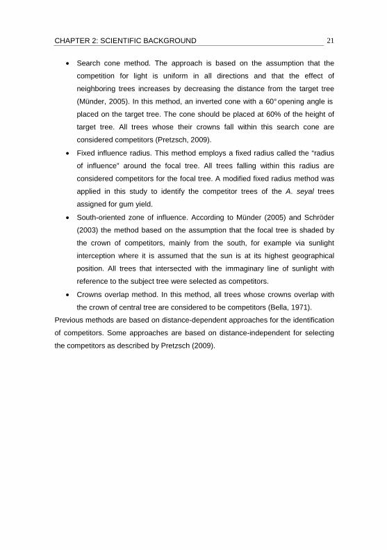
• Search cone method. The approach is based on the assumption that the
competition for light is uniform in all directions and that the effect of
neighboring trees increases by decreasing the distance from the target tree
(Münder, 2005). In this method, an inverted cone with a 60° opening angle is
placed on the target tree. The cone should be placed at 60% of the height of
target tree. All trees whose their crowns fall within this search cone are
considered competitors (Pretzsch, 2009).
• Fixed influence radius. This method employs a fixed radius called the “radius
of influence” around the focal tree. All trees falling within this radius are
considered competitors for the focal tree. A modified fixed radius method was
applied in this study to identify the competitor trees of the A. seyal trees
assigned for gum yield.
• South-oriented zone of influence. According to Münder (2005) and Schröder
(2003) the method based on the assumption that the focal tree is shaded by
the crown of competitors, mainly from the south, for example via sunlight
interception where it is assumed that the sun is at its highest geographical
position. All trees that intersected with the immaginary line of sunlight with
reference to the subject tree were selected as competitors.
• Crowns overlap method. In this method, all trees whose crowns overlap with
the crown of central tree are considered to be competitors (Bella, 1971).
Previous methods are based on distance-dependent approaches for the identification
of competitors. Some approaches are based on distance-independent for selecting
the competitors as described by Pretzsch (2009).

CHAPTER 2: SCIENTIFIC BACKGROUND 22
Source: (Röhle et al., 2003)
Figure 2.4 Methods of selection the competitor trees Where: R = radius; dist = distance; ka = height to the beginning of the crown; h = height; HGK = height to the greatest crown width; VKF = vertical crown area; KF = horizontal crown area; SW = angle of the inverse cone; SH = height to the intersection point; kr = crown radius; OKU = the angle of incidence of
sunlight to crown base of the subject tree.

CHAPTER 3: MATERIALS AND METHODS 23
3 MATERIALS AND METHODS
3.1 Background
This chapter provides an overview of the study area, highlighting the location,
physical attributes, population and land-use patterns. Methods for data collection and
analysis are also described in this chapter.
The current boundaries of South Kordofan state were established by the
Comprehensive Peace Agreement (CPA), which took place in Kenya in 2005
between the Sudanese People Liberation Army (SPLA) and the National Congress
Party (NCP) of the Sudan. South Kordofan is comprised of four main physiographic
regions. These regions are the Nuba Mountains, the eastern plains, the southern
plains, and the western sandy plains. The state (Lat. 9° 50´- 12° 46´ N and Long. 29°
15´- 32° 28´ E), which occupies the south part of G reater Kordofan, has an area of
about 79470 km2. Administratively the state is divided into eight localities; Rashad,
Abu Gibeiha, Talodi, Kadugli, Lagawa, Assalam, Abyei and El Dilling, where Kadugli
is the capital of the state.
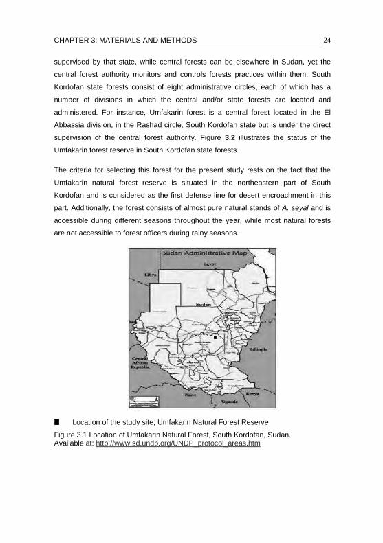
3.2 Study area
This study was conducted in the Umfakarin Natural Forest Reserve (about 540 m
a.s.l, Lat. 12° 29´- 12° 35´ N and Long. 31° 17´ 33 ´´- 31° 20´ E) ( Figure 3.1). This
forest has an area of about 2689 ha and lies 44 km north El Abbassiya town,
belonging to the Rashad locality (7872 km2), South Kordofan state. The forest was
gazetted in 1993 under gazette number (8) and is surrounded by four villages
(Umfakarin, Elhafirah, Elhafirah Dardig and Awlad Rahal). The inhabitants of these
villages mainly depend on the reserved forest for firewood, charcoal, building
materials, grazing, and hunting.
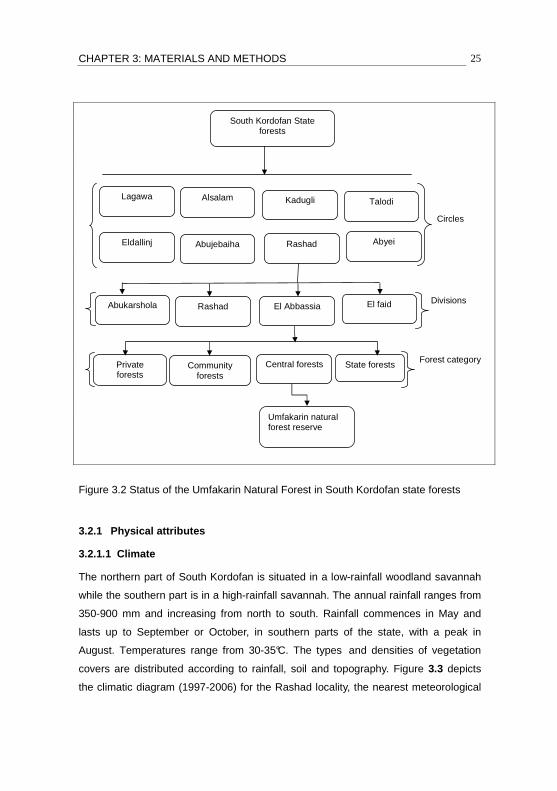
Sudan’s forest legislation recognizes forest ownership as institutional, private and
community forests, in addition to governmental forests, which are either state or
central6 forests. Regional (or state) forests are located in the specified state and are
6
According to the FRA (2010) definition, central forests are forests owned by the central government (federal)
institution (Forests National Corporation). Community forests (social forests) are forests owned by groups of rural population (villagers). Regional (state forests) are forests owned and administrated by the forest authority in that
state. Individual private forests (community) are those which are owned by individuals (one or many). Institutions’ forests are forests owned by agricultural schemes, farmer unions, and companies (private or public).
CHAPTER 3: MATERIALS AND METHODS 24
supervised by that state, while central forests can be elsewhere in Sudan, yet the
central forest authority monitors and controls forests practices within them. South
Kordofan state forests consist of eight administrative circles, each of which has a
number of divisions in which the central and/or state forests are located and
administered. For instance, Umfakarin forest is a central forest located in the El
Abbassia division, in the Rashad circle, South Kordofan state but is under the direct
supervision of the central forest authority. Figure 3.2 illustrates the status of the
Umfakarin forest reserve in South Kordofan state forests.
The criteria for selecting this forest for the present study rests on the fact that the
Umfakarin natural forest reserve is situated in the northeastern part of South
Kordofan and is considered as the first defense line for desert encroachment in this
part. Additionally, the forest consists of almost pure natural stands of A. seyal and is
accessible during different seasons throughout the year, while most natural forests
are not accessible to forest officers during rainy seasons.
Location of the study site; Umfakarin Natural Forest Reserve
Figure 3.1 Location of Umfakarin Natural Forest, South Kordofan, Sudan. Available at: http://www.sd.undp.org/UNDP_protocol_areas.htm
CHAPTER 3: MATERIALS AND METHODS 25
Circles
Divisions
Forest category
Figure 3.2 Status of the Umfakarin Natural Forest in South Kordofan state forests
3.2.1 Physical attributes
3.2.1.1 Climate
The northern part of South Kordofan is situated in a low-rainfall woodland savannah
while the southern part is in a high-rainfall savannah. The annual rainfall ranges from
350-900 mm and increasing from north to south. Rainfall commences in May and
lasts up to September or October, in southern parts of the state, with a peak in
August. Temperatures range from 30-35°C. The types and densities of vegetation
covers are distributed according to rainfall, soil and topography. Figure 3.3 depicts
the climatic diagram (1997-2006) for the Rashad locality, the nearest meteorological
South Kordofan State forests
Lagawa Alsalam
Eldallinj
Kadugli Talodi
Abujebaiha Rashad Abyei
Abukarshola Rashad El Abbassia El faid
Central forests State forests
Umfakarin natural forest reserve
Community
forests
Private forests

CHAPTER 3: MATERIALS AND METHODS 26
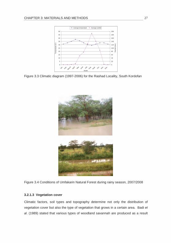
station to the Umfakarin Natural Forest Reserve. This climatic diagram shows the
curves for average monthly temperatures in °C versu s the average monthly rainfall in
mm with a ratio of 1:4. This means, for instance, that the distance along the ordinates
is the same for 20 mm precipitation and 5°C air tem perature (Schultz, 1995). As
described by FAO (2001) and Schultz (1995, 2005) at this ratio, times during which
the precipitation curve is above the temperature curve are considered humid, while
the remaining periods are classified as arid.
Seasonal flooding is the most conspicuous feature in the forest. Every year most
parts of the forest, especially the dense vegetation patches, are inundated for
almost two to four months. Figure 3.4 shows the conditions in the Umfakarin
Reserve Forest during the rainy season 2007/2008.
3.2.1.2 Soil and topography
There are three different main soil types that prevail in South Kordofan; clay plains,
sandy clay (non-cracking soils) locally known Gardud, and sandy soils. The clay
plains comprise about 32 percent while the Gardud and sandy soils comprise about
27 and 21 percent of the total state area, respectively. The rest are rocky soils in hilly
areas and other soils. Clay soils, and to some extent sandy clay and sandy soils, are
suitable for the cultivation of cash crops and basic food staples. Sandy-clay loam,
sandy-loam and Mayaat (soil under water bodies) are the major soil types that prevail
in the Umfakarin Forest Reserve.
In general, the forest reserve can be described as a slightly undulating land surface
with the exception to a few seasonal streams that penetrate some parts of the forest.
No physical features seem to be clearly bounded by the forest reserve or inside the
forest.
CHAPTER 3: MATERIALS AND METHODS 27
Figure 3.3 Climatic diagram (1997-2006) for the Rashad Locality, South Kordofan
Figure 3.4 Conditions of Umfakarin Natural Forest during rainy season, 2007/2008
3.2.1.3 Vegetation cover
Climatic factors, soil types and topography determine not only the distribution of
vegetation cover but also the type of vegetation that grows in a certain area. Badi et
al. (1989) stated that various types of woodland savannah are produced as a result
0
5
10
15
20
25
30
35
40
45
50
Jan.
Feb.
Mar
chApr
ilM
ayJu
neJu
lyAug
.
Sep
t.Oct
.
Nov
.
Dec
.
Month
Te
mp
era
ture
(C
°)
0
20
40
60
80
100
120
140
160
180
200
Ra
infa
ll (
mm
)
Average temperature Average rainfall
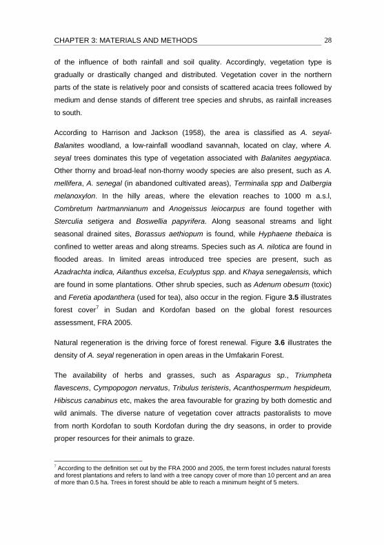
CHAPTER 3: MATERIALS AND METHODS 28
of the influence of both rainfall and soil quality. Accordingly, vegetation type is
gradually or drastically changed and distributed. Vegetation cover in the northern
parts of the state is relatively poor and consists of scattered acacia trees followed by
medium and dense stands of different tree species and shrubs, as rainfall increases
to south.
According to Harrison and Jackson (1958), the area is classified as A. seyal-
Balanites woodland, a low-rainfall woodland savannah, located on clay, where A.
seyal trees dominates this type of vegetation associated with Balanites aegyptiaca.
Other thorny and broad-leaf non-thorny woody species are also present, such as A.
mellifera, A. senegal (in abandoned cultivated areas), Terminalia spp and Dalbergia
melanoxylon. In the hilly areas, where the elevation reaches to 1000 m a.s.l,
Combretum hartmannianum and Anogeissus leiocarpus are found together with
Sterculia setigera and Boswellia papyrifera. Along seasonal streams and light
seasonal drained sites, Borassus aethiopum is found, while Hyphaene thebaica is
confined to wetter areas and along streams. Species such as A. nilotica are found in
flooded areas. In limited areas introduced tree species are present, such as
Azadrachta indica, Ailanthus excelsa, Eculyptus spp. and Khaya senegalensis, which
are found in some plantations. Other shrub species, such as Adenum obesum (toxic)
and Feretia apodanthera (used for tea), also occur in the region. Figure 3.5 illustrates
forest cover7 in Sudan and Kordofan based on the global forest resources
assessment, FRA 2005.
Natural regeneration is the driving force of forest renewal. Figure 3.6 illustrates the
density of A. seyal regeneration in open areas in the Umfakarin Forest.
The availability of herbs and grasses, such as Asparagus sp., Triumpheta
flavescens, Cympopogon nervatus, Tribulus teristeris, Acanthospermum hespideum,
Hibiscus canabinus etc, makes the area favourable for grazing by both domestic and
wild animals. The diverse nature of vegetation cover attracts pastoralists to move
from north Kordofan to south Kordofan during the dry seasons, in order to provide
proper resources for their animals to graze.
7 According to the definition set out by the FRA 2000 and 2005, the term forest includes natural forests
and forest plantations and refers to land with a tree canopy cover of more than 10 percent and an area
of more than 0.5 ha. Trees in forest should be able to reach a minimum height of 5 meters.

CHAPTER 3: MATERIALS AND METHODS 29
In the Umfakarin Forest, vegetation cover is about 75 percent8, A. seyal represents
90 percent. Other woody plants are also found, such as A. mellifera at the forest’s
edge, Balanites aegyptiaca, A. polycantha, A. senegal, A. nilotica in water bodies, A.
sieberana, Cordia Africana, Boscia senegalensis and Dichrostachys cinerea. The
general structure of the Umfakarin Forest can be characterized by either type and/or
the density of its prevailing vegetation. A. seyal of different densities dominates the
forest. In this investigation, these densities can be categorized based on the number
of trees per unit area, or into three strata-dense, medium, and slight, strata. The
existence and diversity of the ground vegetation or understory are determined by the
low density of the tree canopy that allows light to penetrate beneath the canopy.
3.2.2 Population
According to the Sudan population census in 2008, South Kordofan has a population
of 2.3 million persons, representing about 6 percent of the country’s total population.
The state is inhabited by a variety of ethnic groups practicing different livelihoods.
Agriculture, livestock breeding, and the collection of timber and non-timber forest
products are the residents’ main livelihoods.
3.2.3 Land use patterns
The state has a comparative advantage in agricultural and horticultural crops, gum
Arabic and livestock production. Although the state produces a surplus of food and
cash crops, large numbers of inhabitants face food insecure, especially during
rainfall, due to poor infrastructure and limited access to markets. The most important
crops are sorghum, maize, cotton, sesame, millet, fruits, and vegetables. A near-
majority of the population engages in agriculture. Rain-fed cultivation comprises both
smallholder subsistence farming and large-scale mechanized farming. Small irrigated
gardens exist where water is available from seasonal water sources or shallow
aquifers. The total area of land that is suitable for agriculture in South Kordofan is in
the range of 15 million Feddans (1 Feddan = 0.42 ha), of which seven million
Feddans are demarcated and allocated for mechanized farming.
8 Personal communication (September 10, 2007) with H. Elmanzoul (Umfakarin Forest Inspector)

CHAPTER 3: MATERIALS AND METHODS 30
Source: (Dawelbait et al. 2006)
Figure 3.5 Forest cover in Sudan and Kordofan
Figure 3.6 Regeneration of A. seyal in open areas in the Umfakarin Forest, 2007
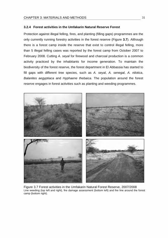
CHAPTER 3: MATERIALS AND METHODS 31
3.2.4 Forest activities in the Umfakarin Natural Reserve Forest
Protection against illegal felling, fires, and planting (filling gaps) programmes are the
only currently running forestry activities in the forest reserve (Figure 3.7). Although
there is a forest camp inside the reserve that exist to control illegal felling, more
than 5 illegal felling cases was reported by the forest camp from October 2007 to
February 2008. Cutting A. seyal for firewood and charcoal production is a common
activity practiced by the inhabitants for income generation. To maintain the
biodiversity of the forest reserve, the forest department in El Abbassia has started to
fill gaps with different tree species, such as A. seyal, A. senegal, A. nilotica,
Balanites aegyptiaca and Hyphaene thebaica. The population around the forest
reserve engages in forest activities such as planting and weeding programmes.
Figure 3.7 Forest activities in the Umfakarin Natural Forest Reserve, 2007/2008 Line weeding (top left and right), fire damage assessment (bottom left) and fire line around the forest camp (bottom right).
CHAPTER 3: MATERIALS AND METHODS 32
3.3 Data collection
Data for this study were collected between September 2007 and February 2008 at
the Umfakarin Natural Forest Reserve, South Kordofan, Sudan.
3.3.1 Reconnaissance survey
The purpose of the reconnaissance survey was to provide a general background
about the area, through observations about the forest under investigation, in terms of
geographical aspects, forest cover, composition, and structure. This survey was
completed in September 2007 by both automobile and foot.
3.3.2 Pre-test samples
Pre-test samples were taken in September 2007 to:
1. Check all the diameter classes. Since A. seyal is a multi-stem species
(McAllan, 1993), usually forking below diameter at breast height (DBH), it was
decided to measure the diameter at a height of 0.25 m to quickly set the
diameter classes. Four classes of diameter were determined; 9-11.5, 13.5-16,
18-20.5 and above 21 cm, based on diameter of 0.25 m height (d0.25). This
criterion was used to determine which trees (subject trees) would be selected
and used in actual field survey of gum talha production.
2. Check the stand densities of natural A. seyal. In this investigation, three stand
density categories, dense, medium and slight, were determined. The dense
stratum, 396 stem/ha on average, is usually inundated for at least two months
during rainy season. However, medium and slight strata, with an average 271
and 209 stem/ha, respectively, are not inundated.
3. Fix the so-called ‘radius of influence’ (ROI) within which neighboring trees
could be identified as competitors for the focal tree.
The term focal, target or subject tree is used in this study to refer to the A. seyal tree,
either tapped by local tools or untapped, selected for gum exudate collection. The
results of pre-test were not incorporated into the results of this study. Two types of
field data were gathered, namely mensurational and gum tapping and collection data.
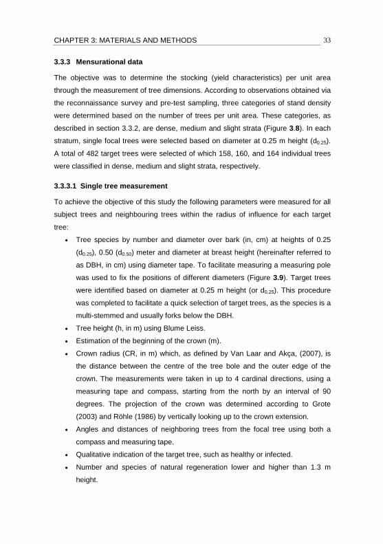
CHAPTER 3: MATERIALS AND METHODS 33
3.3.3 Mensurational data
The objective was to determine the stocking (yield characteristics) per unit area
through the measurement of tree dimensions. According to observations obtained via
the reconnaissance survey and pre-test sampling, three categories of stand density
were determined based on the number of trees per unit area. These categories, as
described in section 3.3.2, are dense, medium and slight strata (Figure 3.8). In each
stratum, single focal trees were selected based on diameter at 0.25 m height (d0.25).
A total of 482 target trees were selected of which 158, 160, and 164 individual trees
were classified in dense, medium and slight strata, respectively.
3.3.3.1 Single tree measurement
To achieve the objective of this study the following parameters were measured for all
subject trees and neighbouring trees within the radius of influence for each target
tree:
• Tree species by number and diameter over bark (in, cm) at heights of 0.25
(d0.25), 0.50 (d0.50) meter and diameter at breast height (hereinafter referred to
as DBH, in cm) using diameter tape. To facilitate measuring a measuring pole
was used to fix the positions of different diameters (Figure 3.9). Target trees
were identified based on diameter at 0.25 m height (or d0.25). This procedure
was completed to facilitate a quick selection of target trees, as the species is a
multi-stemmed and usually forks below the DBH.
• Tree height (h, in m) using Blume Leiss.
• Estimation of the beginning of the crown (m).
• Crown radius (CR, in m) which, as defined by Van Laar and Akça, (2007), is
the distance between the centre of the tree bole and the outer edge of the
crown. The measurements were taken in up to 4 cardinal directions, using a
measuring tape and compass, starting from the north by an interval of 90
degrees. The projection of the crown was determined according to Grote
(2003) and Röhle (1986) by vertically looking up to the crown extension.
• Angles and distances of neighboring trees from the focal tree using both a
compass and measuring tape.
• Qualitative indication of the target tree, such as healthy or infected.
• Number and species of natural regeneration lower and higher than 1.3 m
height.
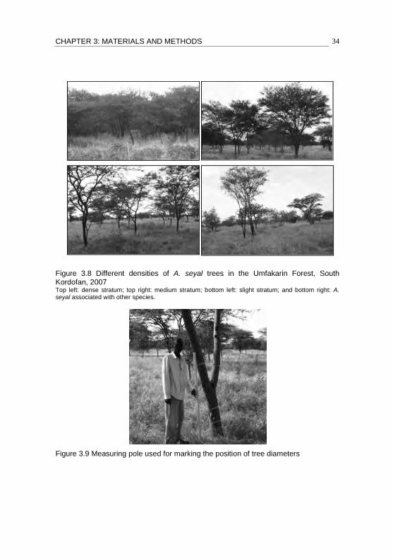
CHAPTER 3: MATERIALS AND METHODS 34
Figure 3.8 Different densities of A. seyal trees in the Umfakarin Forest, South
Kordofan, 2007 Top left: dense stratum; top right: medium stratum; bottom left: slight stratum; and bottom right: A. seyal associated with other species.
Figure 3.9 Measuring pole used for marking the position of tree diameters

CHAPTER 3: MATERIALS AND METHODS 35
3.3.3.2 Identifying the competitors
Normally when measuring trees in a stand, sample plots of a specific radius are
distributed systematically or randomly within the forest stand. In this study, each
sample has a different radius referred to as the radius of influence (ROI) or the radius
of influence zone (RIZ). These terms are frequently used in forest growth and
measurement for the calculation of competition indices (CIs) as a measure of the
competition between trees in forest stands. In previous studies, the criteria for
determining RIZ, and thus the competitors, was based on different methods. For
example, Arney (1973) used the radius of influence equivalent to open-grown crown
radius of Douglas-fir trees on the Pacific coast. While Hegyi (1974), includes all
competitors within a radius of ten feet (3.05 m). In the present study, a different
approach was adopted to select competitor trees, as trees have different forms,
especially the tropical dry ones such as A. seyal in Sudan. The criterion for
identifying competitors was based on the height of the subject tree. The radius of
influence was determined after several attempts in pre-test sampling. This radius of
the circle is a function of tree size (Gadow and Hui, 1999). The suitable influence
zone used to identify competitors was defined as the radius of a circle equal to the
height of subject tree multiplied by a factor (1.25), r = h*1.25, where r is the radius of
influence (in, m) and h is tree height (in, m). All trees falling within this radius were
considered to be competitors of the focal tree. Several characteristics such as DBH,
tree height, height to the crown base, and crown radii of target tree and its
competitors beside competitors coordinates were measured and incorporated into
the computation of the competition indices.
3.3.3.3 Tree mapping
Polar coordinates were used to describe the position of individual trees in each
sample plot. Within the radius of influence, trees were mapped using the subject tree
as a focal point. Figure 3.10 shows the distribution of neighbourhood trees, whereby
the distance from the target tree fell within an area of 380.13 m2 (radius or r = 11 m).
Mapping the locations of neighbourhood trees was carried out according to Dimov
(2004), by measuring the angle from the north using a compass and the horizontal
distance (m) to each tree from the subject tree. Appendix 1 shows the form used for
tree measurements and tree mapping.
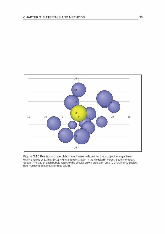
CHAPTER 3: MATERIALS AND METHODS 36
Figure 3.10 Positions of neighborhood trees relative to the subject A. seyal tree within a radius of 11 m (380.13 m²) in a dense stratum in the Umfakarin Forest, South Kordofan, Sudan. The size of each bubble refers to the circular crown projection area (CCPA, in m²). Subject
tree (yellow) and competitor trees (blue).
-15
-10
-5
0
5
10
15
-15 -10 -5 0 5 10 15
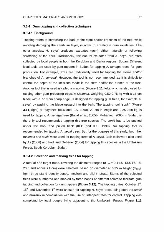
CHAPTER 3: MATERIALS AND METHODS 37
3.3.4 Gum tapping and collection techniques
3.3.4.1 Background
Tapping refers to scratching the bark of the stem and/or branches of the tree, while
avoiding damaging the cambium layer, in order to accelerate gum exudation. Like
other acacias, A. seyal produces exudates (gum) either naturally or following
scratching of the bark. Traditionally, the natural exudates from A. seyal are often
collected by local people in both the Kordofan and Darfur regions, Sudan. Different
local tools are used by gum tappers in Sudan for tapping A. senegal trees for gum
production. For example, axes are traditionally used for tapping the stems and/or
branches of A. senegal. However, the tool is not recommended, as it is difficult to
control the depth of the incisions made in the stem and/or the branch of the tree.
Another tool that is used is called a makmak (Figure 3.11, left), which is also used for
tapping other gum producing trees. A Makmak, weighing 0.50-0.75 kg with a 15 cm
blade with a 7-10 cm sharp edge, is designed for tapping gum trees, for example A.
seyal, by pushing the blade upward into the bark. The tapping tool “sonki” (Figure
3.11, right) or “bayonet” (IIED and IES, 1990), 20 cm in length and 0.25-0.50 kg, is
used for tapping A. senegal tree (Ballal et al., 2005b; Mohamed, 2005) in Sudan, is
the only tool recommended tapping this tree species. The sonki has to be pushed
under the bark and pulled back (IIED and IES, 1990). No tapping tool is
recommended for tapping A. seyal trees. But for the purpose of this study, both the,
makmak and sonki were used for tapping trees of A. seyal. Both tools were also used
by Ali (2006) and Fadl and Gebauer (2004) for tapping this species in the Umfakarin
Forest, South Kordofan, Sudan.
3.3.4.2 Selection and marking trees for tapping
A total of 482 target trees, covering the diameter ranges (d0.25 = 9-11.5, 13.5-16, 18-
20.5 and above 21 cm) were selected, based on diameter at 0.25 m height (d0.25),
from three stand density-dense, medium and slight- strata. Stems of the selected
trees were numbered and marked by three bands of different colors to facilitate gum
tapping and collection for gum tappers (Figure 3.12). The tapping dates, October 1st,
15th and November 1st were chosen for tapping A. seyal trees using both the sonki
and makmak in combination with the use of untapped trees for control. Tapping was
completed by local people living adjacent to the Umfakarin Forest. Figure 3.13

CHAPTER 3: MATERIALS AN
illustrates the gum tapping a
from tapped and untapped tre
Source: Adapted from Ali, 2006
Figure 3.11 Local tools used f
(Makmak and sonki, from left t
ND METHODS
nd collection techniques in addition to gu
es.
for tapping Acacia seyal for gum production
to right)
38
m exudation

CHAPTER 3: MATERIALS AND METHODS 39
Figure 3.12 Techniques for marking Acacia seyal trees for gum tapping Top right: (yellow band) for sonki; bottom left: (red band) for makmak; and bottom right: blue band for untapped trees.

CHAPTER 3: MATERIALS AND METHODS 40
Figure 3.13 Acacia seyal: gum tapping and collection techniques Top left: tapping techniques; top right: gum collection; bottom left: natural gum exudation; and bottom
right: gum exudation after tapping.
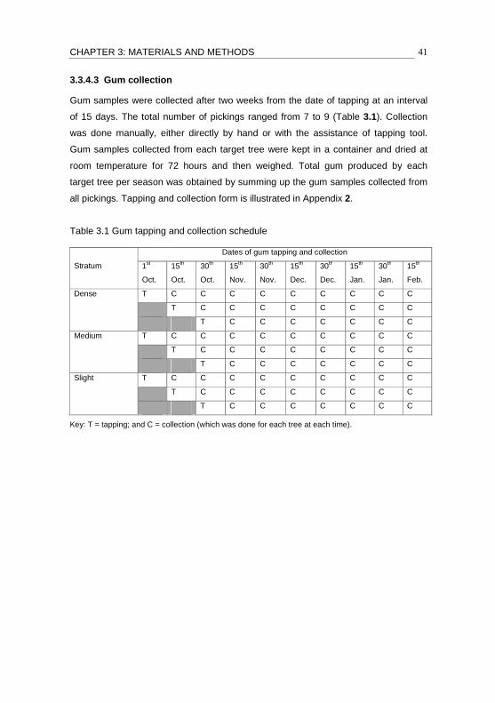
CHAPTER 3: MATERIALS AND METHODS 41
3.3.4.3 Gum collection
Gum samples were collected after two weeks from the date of tapping at an interval
of 15 days. The total number of pickings ranged from 7 to 9 (Table 3.1). Collection
was done manually, either directly by hand or with the assistance of tapping tool.
Gum samples collected from each target tree were kept in a container and dried at
room temperature for 72 hours and then weighed. Total gum produced by each
target tree per season was obtained by summing up the gum samples collected from
all pickings. Tapping and collection form is illustrated in Appendix 2.
Table 3.1 Gum tapping and collection schedule
Stratum
Dates of gum tapping and collection
1st
Oct.
15th
Oct.
30th
Oct.
15th
Nov.
30th
Nov.
15th
Dec.
30th
Dec.
15th
Jan.
30th
Jan.
15th
Feb.
Dense T C C C C C C C C C
T C C C C C C C C
T C C C C C C C
Medium T C C C C C C C C C
T C C C C C C C C
T C C C C C C C
Slight T C C C C C C C C C
T C C C C C C C C
T C C C C C C C
Key: T = tapping; and C = collection (which was done for each tree at each time).

CHAPTER 3: MATERIALS AND METHODS 42
3.4 Computational statistics of tree and stand values
Quadratic mean diameter (QMD, in cm), mean height, basal area per hectare,
number of trees/ha, standing volume per hectare, and crown parameters were
computed for trees in each stratum, as follows:
• Quadratic mean diameter
The quadratic mean diameter, i.e. diameter at breast height (DBH) corresponding to
the average basal area of trees in the stand was obtained (Formula 4) according to
Kramer and Akça (2008), Vink (1990b) and West (2004).
� � �∑��
�
�
�
��� .......................................................................................................... (4)
Where � is the quadratic mean diameter (QMD, in cm); � is the number of observations; and �� is the
diameter at breast height (DBH, in cm) of �, tree.
• Stand basal area
Basal area per hectare was calculated by multiplying the mean diameter with number
of trees per hectare (Formula 5).
�� � � �²/40000 ................................................................................. (5)
Where �� is the basal area per hectare (m²); � is the QMD; and � represents the number of trees per
hectare and represents 3.14159265.
• Stand mean height
The mean height of the stand was calculated following Kramer and Akça (2008) and
Van Laar and Akça (2007) by regressing the Michailow stand height curve on the
mean DBH (Formula 6).
)/(0
1*3.1 DaeaH +=.................................................................................................... (6)
Where H is the mean height (m); D is the QMD; e is the base of natural logarithm; and 0a and 1arepresent coefficients.
• Single tree volume was obtained using Formula 7, as illustrate below:
ffhbav **= ………………………………………………………………………………. (7)
Where ba represents the tree’s basal area (in m2, 40000/*2 πdba= ); d represents tree diameter
(DBH); h represents the observed tree height (m); ff is the form factor ( ff = 0.5 according to El Dool,
1988); and = 3.14159265.
• Standing volume
The Stand-level volume equation (Gadow and Hui 1999) was used to derive the
standing volume in m³/ha:
� � �� � ��......................................................................................................... (8)

CHAPTER 3: MATERIALS AND METHODS 43
Where is volume in m³/ha; ��, � and �� represent Basal Area, height and form factor, respectively.
• Crown parameters
The measured four crown radii were used to calculate the average crown radius (CR,
in m) and the crown projection area (CrPA, m²). The CR, which is equal to ½ the
crown diameter (CD, in m) was obtained by calculating the arithmetic mean of the
four radii. Two crown shapes, i.e. circle and ellipse, were assumed for A. seyal for
the calculation of CrPA. CrPA of either a circle or ellipse for the individual trees was
calculated according to the equations (9) and (10).
Circular crown area:
π*)4
( 24321 rrrrCrPA
+++= ……………………………………………………...………… (9)
Elliptic crown area:
( ) 4/*)*()()*()*( 144*33221 πrrrrrrrrCrPA +++= ………………………………….….….. (10)
Where: CrPA= crown projection area (m2); 41...rr = crown radii (m); and represents 3.14159265.
3.4.1 Stand height curve
Height-diameter relationship was evaluated using several height functions (Table 3.2)
based on data from medium stand density (Kramer and Akça, 2008). The criteria for
selecting the best model to be used for the A. seyal height curve were based on R²,
Akaike’s Information Criterion (AIC) and plausibility of the curve. Stand height curves
were produced for dense, medium, and slight strata using the selected allometric
height function.
Table 3.2 Potential models used for evaluation of height-diameter relationship of A. seyalFunction name Function Parabolic 2
210 ** dadaah ++=
Petterson
2
10 *3.1
⎟⎟
⎠
⎞
⎜⎜
⎝
⎛
++=
daad
h
Prodan )**/(3.1 2210
2 dadaadh +++=Michailow )/(
01*3.1 daeah +=
Hendrickson daah log*10 +=Van Laar )//( 2
210 dadaaeh ++=Source: (Kramer and Akça, 2008)
Where: h = total height (m); d = diameter at breast height (DBH, in cm); log = natural logarithm; e =
base of natural logarithm (≈ 2.7183); a0, a1 and a2 are coefficients. Observations (n = 1235) based
on data from medium stratum.
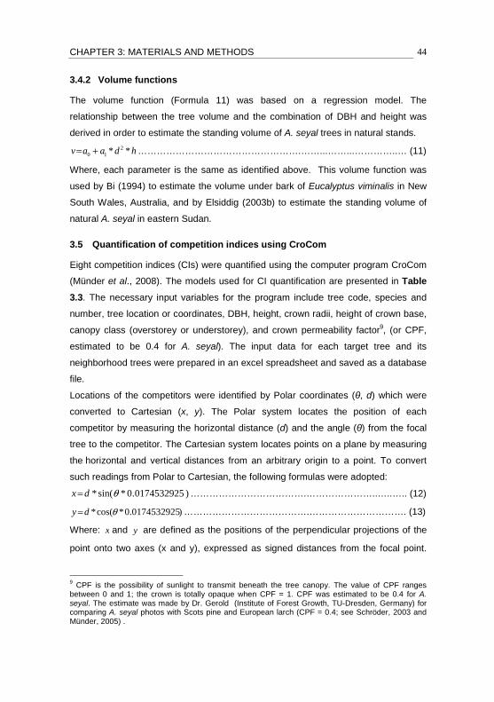
CHAPTER 3: MATERIALS AND METHODS 44
3.4.2 Volume functions
The volume function (Formula 11) was based on a regression model. The
relationship between the tree volume and the combination of DBH and height was
derived in order to estimate the standing volume of A. seyal trees in natural stands.
hdaav ** 210 += …………………………………………….……...……...…………..… (11)
Where, each parameter is the same as identified above. This volume function was
used by Bi (1994) to estimate the volume under bark of Eucalyptus viminalis in New
South Wales, Australia, and by Elsiddig (2003b) to estimate the standing volume of
natural A. seyal in eastern Sudan.
3.5 Quantification of competition indices using CroCom
Eight competition indices (CIs) were quantified using the computer program CroCom
(Münder et al., 2008). The models used for CI quantification are presented in Table
3.3. The necessary input variables for the program include tree code, species and
number, tree location or coordinates, DBH, height, crown radii, height of crown base,
canopy class (overstorey or understorey), and crown permeability factor9, (or CPF,
estimated to be 0.4 for A. seyal). The input data for each target tree and its
neighborhood trees were prepared in an excel spreadsheet and saved as a database
file.
Locations of the competitors were identified by Polar coordinates (θ, d) which were
converted to Cartesian (x, y). The Polar system locates the position of each
competitor by measuring the horizontal distance (d) and the angle (θ) from the focal
tree to the competitor. The Cartesian system locates points on a plane by measuring
the horizontal and vertical distances from an arbitrary origin to a point. To convert
such readings from Polar to Cartesian, the following formulas were adopted:
)0174532925.0*sin(* θdx = ……………………………….…………………..…..….. (12)
)0174532925.0*cos(* θdy = ………………………………….…………………………. (13)
Where: x and y are defined as the positions of the perpendicular projections of the
point onto two axes (x and y), expressed as signed distances from the focal point.
9 CPF is the possibility of sunlight to transmit beneath the tree canopy. The value of CPF ranges
between 0 and 1; the crown is totally opaque when CPF = 1. CPF was estimated to be 0.4 for A. seyal. The estimate was made by Dr. Gerold (Institute of Forest Growth, TU-Dresden, Germany) for comparing A. seyal photos with Scots pine and European larch (CPF = 0.4; see Schröder, 2003 and
Münder, 2005) .

CHAPTER 3: MATERIALS AND METHODS 45
The constant (0.0174532925) was used to transform the compass readings from
“degrees” to “radians” (1 degree = 0.0174532925 radian); d and θ represent
horizontal distance and angle (compass reading) of the competitor from the focal
tree, respectively.
The results of the data analyzed by CroCom create intra- and inter-specific
competition indices. According to the CroCom definition, the intra-specific
competition expresses the competition between trees sharing the same crown layer,
while inter-specific competition exists between trees growing at different layers.
However, in ecology, inter-specific competition refers to the competition that occurs
whenever two different species attempt to utilize the same limited resources, while
intra-specific is the competition between individuals of the same species (Kimmins,
2004; Begon et al., 2006). To avoid confusion between these two concepts, in
CroCom and ecology, intra- and inter-layer competitions will be used to refer to the
competition between trees sharing the same layer and the competition between trees
growing in different layers, respectively. The final competition index induced by the
competitors is the sum of inter- and intra-layer competition.
Table 3.3 Models used for CIs quantification in CROCOM Programme Index formula Variables used in the model Author (s)
Distance-dependent competition indices
∑=
=nj
jijij distddHEGYICI
1
)/()/(_DBH, distance Hegyi 1974
∑=
+=nj
jijij distggHEGYICI
1
)1/()/(2__Basal area, distance Hegyi 1974
∑=
=nj
j i
j
KF
SHKFKFCI
1
)(_
Crown dimensions Biging and Dobbertin 1992
∑=
=nj
j i
j
KV
SHKVKVCI
1
)(_
Crown dimensions Biging and Dobbertin 1992
ji
ij
nj
j
KQFKQFBetaPRETZSCHCI /*_1
∑=
=Angle of inverse cone and
crown dimensions
Pretzsch 1995
∑= +
=nj
j ij
ij
dist
VKFVKFVKFCI
1 1
/_
Crown dimensions and distance
Münder und Schröder 2001
Distance-independent indices
∑=
=nj
jHGKj i
KFCCI1
)(66_Crown dimensions Nagel 1999
∑=
==max
1
_n
jjcum gGBALCI
Basal area Wykoff et al. 1982; Schütz
2001; Schütz und Röhnisch 2003
Source: (Scütz 2001; Schütz and Röhnisch 2003; Schröder 2003; Münder 2005; Rivas et al. 2005) Where: i = focal tree; j = competitor; d = diameter at breast height (DBH); dj max = DBH of trees larger
than the subject tree (in cm); BAL = basal area of trees larger than the subject tree (m2/ha); ig = basal
area (BA, in m²); Gcum = cumulative BA of trees larger than the subject; nmax= number of trees of basal areas larger than the subject tree; nj= number of competitors; distij= distance treei- treej; Beta =

CHAPTER 3: MATERIALS AND METHODS 46
gradient of straight line connecting base of search cone and top of competitor tree; KF = horizontal crown area; KQF= KF at height of search-cone base; HGK = height of greatest crown width; SH = height of intersection of search cone and tree axis; KV= crown volume; VKF = vertical crown area; and h = height.
Definition of indices used in CroCom:
Distance-dependent competition indices
1. CI_HEGYI (Hegyi, 1974): also known as the "Jack-Pine-index" was discovered
in 1974 by Hegyi and is considered to be the most famous and easiest index
(Münder, 2005; Schröder, 2003) to use to quantify competition indices in forest
stands. The index is only based on DBH of both the target tree and its
competitors and the horizontal distance between each competitor and the
target tree.
2. CI_HEGYI_2 (Hegyi 1974): similar to first index but employs basal area
instead of diameter.
3. CI_KF (Biging and Dobbertin, 1992): based on the horizontal crown area and
the height of intersection of the search cone and tree axis.
4. CI_KV (Biging and Dobbertin, 1992): the index uses crown volume based on
the height of intersection of the search cone and tree axis.
5. CI_PRETZSCH (Pretzsch, 1995): this index is a component of the forest
growth simulator, SILVA, developed at the Chair of Forest Yield Science at the
Technical University of Munich, Germany. It is used to quantify the competition
index based on the identification of competitors by means of the search cone
method.
6. CI_VKF (Münder and Schröder, 2001): this index is based on the vertical
crown area and horizontal distance between the competitor and subject tree.
Distance-independent competition indices
�� CI_C66 (Nagel 1999): based on the horizontal crown area at the height of
greatest crown width. The C66 of a subject tree is calculated by summing up
the horizontal crown areas of all trees cut at the height of its greatest crown
width, which is fixed at 66.6% of crown length from the top (Nagel 1999 in
Schröder et al., 2007). The C66 index identifies competitors either as all trees
belonging to the same stand (distance-independent mode) or by checking a

CHAPTER 3: MATERIALS AND METHODS 47
fixed critical radius (distance-dependent mode) (Schröder et al., 2007). The
latter was used in this study to identify competitors.
�� CI_BAL (Wykoff et al., 1982): this index is also termed the “Gcum” or shading
index (Schütz, 2001; Schütz and Röhnisch, 2003) and can be calculated by
summing up the basal areas of the trees larger (BAL) than the subject tree.
3.6 Statistical analysis
3.6.1 Test for normality
The test for normality is an important procedure for testing the null hypothesis that
the data sample came from a normally distributed population. Many statistical
procedures are used for testing departures from normality. In this study, normality
plots with tests (Kolmogorov-Smirnov or Shapiro-Wilk) were used to test whether the
data have come from a normally distributed population. In this investigation the
goodness of fit, for example Shapiro-Wilk test (Zar, 2009), was selected. If a test of
significance gives a p-value greater than the chosen alpha level (in this case α =
0.05), then one can conclude that the data came from a normally distributed
population. The Shapiro-Wilk test statistic (W) is calculated as follows (Sachs and
Hedderich, 2006):
W �
�∑ ������
�²�
���
∑ ������
��
���
…………………………………….…………………………………… (14)
Where:
���
� ��…�
�� is the �� ordered sample values (�
�� is the smallest value); �
� ��
…�
�� are
constants obtained from the measures of order statistics of a normally distributed random variables; �
is the sample mean; and is the sample size.
3.6.2 Simple linear correlation
The simple linear correlation considers the linear relationship between two variables
(x and y), but neither is assumed to be functionally dependent upon the other (Van
Laar and Akça, 2007; Zar, 2009). The correlation coefficient (r) is the most important
parameter to be determined in simple linear correlation. There are several different
correlation methods, but the most common type is the Pearson, or product moment,
correlation. The relationship between two variables when removing the influence of
other variables is referred to as a partial correlation. The value of r ranges between 1
and -1, or -1<r<+1. As indicated by Zar (2009), a positive correlation implies that if

CHAPTER 3: MATERIALS AND METHODS 48
one variable increases in value then the other variable also increases in value; a
negative correlation indicates that an increase in value of one of the variables will be
accompanied by a decrease in value of the other variable. If r = 0, there is no linear
association between the two variables. The mathematical formula for computing the
correlation coefficient (r) is provided by Zar (2009), as depicted in Formula (15):
⎟
⎟
⎠
⎞
⎜
⎜
⎝
⎛
−⎟
⎟
⎠
⎞
⎜
⎜
⎝
⎛
−
−=
∑∑
∑∑
∑ ∑∑
n
yy
n
xx
n
yxxy
r2
22
2 )()(
……………………………………….………. (15)
Where: r = correlation coefficient; x and y = are dependent and independent variables, respectively; and n = number of observations.
3.6.3 Regression analysis
Regression analysis is useful for evaluating the association between two or more
variables and expressing the nature of such relationships (Husch et al., 2003).
Regression is either simple, if only two variables are considered, or multiple, if more
than two variables are considered. The simplest relationship between one dependent
and one independent variable, for example a simple linear regression, is illustrated
below in Equation 16. However, when a number of predictors (independent variables)
influence the dependent variable (Zar, 2009) the situation is best expressed by
Equation 17.
iii xaay ε++= 10ˆ ………………………………………………………..……………..…. (16)
inni xaxaxaay ε+++++= ...ˆ 22110 ……………………..…………………………….…… (17)
Where: iy is the dependent or response variable (predicted value); nxxx ..., 21 are independent or
explanatory variables; 0a is the intercept and also denotes the expected value of dependent variable
when the independent(s) variable(s) is zero; naaa ..., 21 are parameters to be estimated by linear
regression: and iε represents the error or residual which is the difference between the predicted value
and the observed value of the response variable.
Generally, a nonlinear regression represents any regression in which the relationship
between the dependent and independent variable(s) is not linear. Regression models
such as logarithmic, exponential or any forms in which the estimated parameters do
not appear in an additive manner are examples of nonlinear regression. The normal
nonlinear regression model (Equation 18) can be written as:
iii xfy εβ += ),( ´………………………………………………………………….………. (18)
CHAPTER 3: MATERIALS AND METHODS 49
Where: iy = ( nyy ...1 ) is a vector of predictors for the thi of n observations;
´ix = )...( 1 nxx is a vector of
explanatory variable; β = )...( 1 naa is a vector of parameters to be estimated by non-linear regression;
and iε = random error, iε ~ N (0, σ²).
Some examples of non-linear regression models (Equations 19-21) used in this study
are depicted below.
)ln(*10 xaay += ………………………………………………………………….…….. (19)
xaay 10 *= …………………………………………………….…………………..……… (20)
)/(0
1* xaeay = …………………………………………………………………........…. (21)
Where: y represents the outcome variable; x illustrates the explanatory variable; ln represents a
natural logarithm; e is the base of natural logarithm and is approximately equal to 2.7183; 10 aandadenote parameters to be estimated by regression model; and ε refers to error.
The most important parameter to be determined by regression analysis is the
coefficient of determination (or R²). The coefficient of determination (0 ≤ R² ≤ +1)
quantifies the regression’s goodness of fit which indicates how suitable the model is
for the data presented. R² is sometimes referred to as expressing the goodness of fit
of the line for the data or as the precision of the regression (Zar, 2009). R² also
measures the proportion (or percentage) of the total variation in response variables
as explained by the regression model. When new explanatory variables are added to
a regression equation, R² may increase even if the new variables have no predictive
capability. Unlike R², adjusted R² (R²adj) may not increase unless the new variables
have a real predictive capability. R² and R²adj can be calculated using the Equations
depicted in 22 and 23.
∑
∑
=
=
−
−−= n
ii
n
iii
yy
yyR
1
2
1
2
2
)(
)ˆ(1 ……………………………………………………………………... (22)
1)1(* 2
22
−−−−=kn
RkRR adj …………………………………………………………………... (23)
Where: R² is the coefficient of determination; R²adj represents the adjusted R²; iy depicts the observed
values from ni ...1= ; iy denotes predicted values; iy is the average value of iy ; k is the number of
parameters; and n represents the number of observations.

CHAPTER 3: MATERIALS AND METHODS 50
The standard error of the estimate (SE) is another parameter used to measure the
accuracy of predictions originating from a regression analysis. SE is indicated as the
root of the mean square error (MSE) and can be calculated using the following
formula:
MSEorkn
yySE ii
−−
= ∑2)ˆ(
…………………………………………….…………..….. (24)
Where: SE is the standard error of the estimate; MSE is the mean square error; and iyk, , iy and nrepresent the variable depicted in the equation above.
Akaike’s Information Criterion (AIC)
AIC is an index proposed by Akaike (1974) to measure the fit of the model (Burnham
and Anderson, 2002). The AIC is recently used for judging the performance of
several candidate models. The minimum value of the index, the adequate model fit to
the data. The mathematical formula for calculating AIC is as follows:
��� � 2� � ln �����………………………………………………………………….. (25)
Where: AIC is Akaike’s Information Criterion; k is the number of parameters in the model; n is number
of observations; ln is the natural logarithm; RSS is the residual sum of squares.
Transformation of non-linear into linear regression models
Some non-linear models can be transformed into linear versions. In this study, and
for the sake of testing the significance of the regression lines, non-linear regression
models such as equations 26 and 27 were transformed into a linear form, using a
logarithmic transformation. The two models were transformed as follows:
10 log*log)log( axay ii += ……………………………………………...…..…………… (26)
ii xaay /log)log( 10 += …………………………….…………………………..…………. (27)
Where: log is the logarithm to the base 10; and yi, xi, 0a and 1a are as previously explained.
Test of significance between regression lines
There are three possible comparisons for testing the significance between linear
regression lines (Glantz, 2005):
- test for a difference in slope (regardless of the intercepts)
- test for a difference in intercept (regardless of the slopes)
- overall test of coincidence, in which if the lines are different.
CHAPTER 3: MATERIALS AND METHODS 51
This study deals only with the first option, the test of differences in slope regardless
of the intercepts. A simple method for testing the hypothesis whether the slopes of
two regression lines are different or not (H0: b1=b2) has been identified by many
authors (see e.g. Glantz, 2005; Husch, 1963; Zar, 1999). The procedure for
comparing the two slopes is analogous to the t test for differences between two
means. The mathematical term or the test statistic is:
21
21
bbSbb
t−
−= ………………………………………………………………………….….…… (28)
Where the standard error of the difference between regression coefficients is:
∑∑
+=−2
2
.2
12
.2
)(
)(
)(
)(21 x
S
x
SS pxypxy
bb ……………………………………………………...…...…. (29)
The pooled residual mean square is calculated as:
21
21.
2
)()()()(
)(DFresidualDFresidualSSresidualSSresidual
S pXY++= ……………………………………..…...….. (30)
The critical value of the t for this test has )4( 21 −+ nn degrees of freedom (where n1
and n2 are the number of observations for lines 1 and 2 respectively). To compare
several regression lines (H0: ß1 = ß2 = … = ßk, where k is the number of lines needed
to be tested), an analysis of covariance has to be used (Zar, 1999). F statistic can be
calculated using the following formula:
)/()1
(p
ppc
DF
SS
k
SSSSF
−−
= …………………………………………………………………... (31)
Where:
SSc is the common residual sum of squares; SSp is the pooled residual sum of squares; and DFp is the
residual degrees of freedom.
The steps taken to calculate SSc, SSp and DFp are shown in the following table
(Table 3.4).

CHAPTER 3: MATERIALS AND METHODS 52
Table 3.4 Calculations for testing significant differences between slopes of kregression lines
∑x² ∑xy ∑y² RSS RDF
Regression 1
Regression 2 . . Regression k
Pooled regression
Common regression
A1
A2
.
. Ak
∑=
=k
iic AA
1
B1
B2
.
. Bk
∑=
=k
iic BB
1
C1
C2
.
. Ck
∑=
=k
iic CC
1
12
111 / ABCSS −=
22222 / ABCSS −=
.
.
kkkk ABCSS /2−=
∑=
=k
iip SSSS
1
cccc ABCSS /2−=
211 −= nDF
222 −= nDF. .
2−= kk nDF
∑=
−=k
iip nDF
1
)2(
∑=
−−=k
iic knDF
1
1
Source: (Zar, 1999)
Logistic regression
Logistic regression, or sometimes the logistic model, is used for the prediction of the
probability of occurrence of an event. The difference between the logistic model and
the linear regression model is that the outcome variable in a logistic regression is
binary or dichotomous (Hosmer and Lemeshow, 2000; Zar, 1999). The dependent
variable has two possible values, for example yield or no yield, male or female, or
more, for example low, medium, and high. The independent variable(s) can be
measurable and/or categorical. In this study, a binary logistic regression was used to
describe the relationship between the dependent variable (gum yield) and the
independent variables (stand density, tapping tool, tapping date, DBH and
competition index value). The dependent variable (dichotomous) was set as 1 and 0
referring to yield and no gum yield. In this case, the mathematical expression of
logistic model can be written as follows:
)1
1/(1 )...22110 nn xaxaxaaey ++++= …………………………………………………………..…… (32)
Where: y is the probability of gum yield; other variables are defined as explained previously.
The Wald 2χ statistic is used to test the significance of each variable´s coefficient in
the model and can be calculated by squaring the quotient of the coefficient divided by
its standard error, compared with a tabulated 2χ with 1 degree of freedom under a
certain level of significance (α = 0.05).

CHAPTER 3: MATERIALS AND METHODS 53
3.6.4 Post-Hoc tests in the analysis of variance (ANOVA)
Post-hoc tests are generally performed only after obtaining a significant difference
between the means of several treatments and where additional exploration is needed
to provide specific information about the reason why the means are significantly
different from each other. In this study, an ANOVA test was applied in order to test
whether the means of gum yield obtained from different gum tapping treatments are
equal or not. In addition to that, Post-hoc in ANOVA, based on the Scheffé test, was
applied to make simple comparisons of all possible pair-wise gum yield means. The
Scheffé test (S test) can be used to test the null hypothesis of the form
0:0 =− ABH μμ (Zar, 1999), where Bμ and Aμ are the values of the two means. The
important parameters to be quantified when conducting Scheffé test (S test), are the
test statistics (S), and the critical value of S. The mathematical breakdown of S
statistic is:
SEXX
SAB ||
−−−= ………………………………………………………………………..….. (33)
Where:
⎟⎟
⎠
⎞
⎜⎜
⎝
⎛
+=BA nn
SSE112 ……………………………………………………………………..... (34)
And the critical value is:
.,1,)1( kNkFkS −−−= αα …………………………………………………………………….. (35)
Where: S is the Scheffé test statistics; −−
BA XandX represent the mean values of treatments A and B
respectively; SE denotes the Standard error; αS is the critical value of S; BA nandn are the number
of observations in treatments A and B , respectively; k is equal to the number of treatments; Nrepresents the number of observations in all treatments; and αF represents the tabulated Fisher value
(in this case α = 0.05) under ,1−k and kN − degrees of freedom.
To accept or reject the null hypothesis depends on the αS value. If αS < S statistics
the null hypothesis should be rejected and if it is not then the hypothesis is acceptable.
CHAPTER 3: MATERIALS AND METHODS 54
3.6.5 Regression tree
Classification and Regression Trees (CART) is a package available in R software via
the user-contributed packages rpart and tree (R Development Core Team, 2008;
Venables et al., 2009). The classification tree is mainly used for predicting categorical
dependent variables, while the regression tree is used to predict continuous
dependent variables (Cappelli and D’Elia, 2006). In this study, the regression tree
was applied to predict gum talha productivity based on a set of explanatory variables.
Tree-based models are computationally intensive methods that are used in situations
where there are many explanatory variables and the aim is to identify which of them
can be included in a regression model (Crawley, 2007), and to find interaction
variables (Faraway, 2006). Tree-based methods are non-parametric tools that allow
modelling the relationship between a response variable and a set of predictors by
means of a recursive binary partitioning approach (Cappelli and D’Elia, 2006). The
advantages of tree-based methods which can be summarized by the following
(Crawley, 2007):
• They are very simple.
• They are excellent for initial data inspection.
• They provide a very clear picture of the structure of the data.
• They provide a highly intuitive insight into the types of interactions that exist
between variables.
In a regression tree, the response variable is a continuous measurement, whereas
explanatory variables can be any mix of continuous and categorical variables
(Crawley, 2007). In this study, the model is fitted using a regression tree by stating
that gum yield (response variable) is a function of several explanatory variables,
including stand density, tapping tool, date of tapping, tree competition and DBH.
The data frame containing all variables, for example response and predictors, were
prepared in an excel worksheet and saved in a pure text format, for example comma-
separated value (CSV). The prepared file can be loaded directly into R as a data
frame, using the “read.table” function. To run the program, the user must type some
commands, such as the command “print” which shows the summary statistics for the
model, contains the node number, the split, the number of observations per node,
deviance, and the mean value of the response variable at each terminal node. As
explained by Crawley (2007), in the command “print” of the regression tree model,
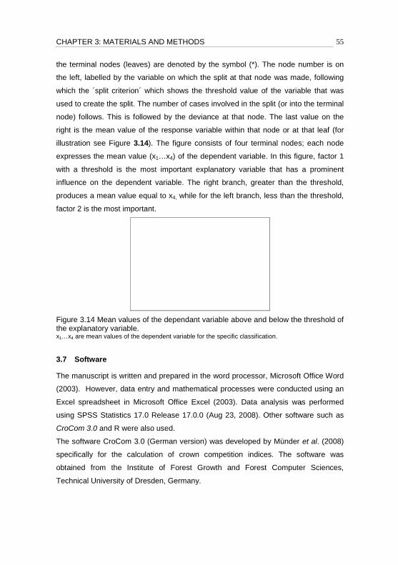
CHAPTER 3: MATERIALS AN
the terminal nodes (leaves) a
the left, labelled by the variab
which the ´split criterion´ whic
used to create the split. The n
node) follows. This is followe
right is the mean value of the
illustration see Figure 3.14).
expresses the mean value (x
with a threshold is the most
influence on the dependent v
produces a mean value equa
factor 2 is the most important.
Figure 3.14 Mean values of ththe explanatory variable. x1…x4 are mean values of the depen
3.7 Software
The manuscript is written and
(2003). However, data entry
Excel spreadsheet in Microso
using SPSS Statistics 17.0 R
CroCom 3.0 and R were also
The software CroCom 3.0 (Ge
specifically for the calculatio
obtained from the Institute
Technical University of Dresde
ND METHODS
are denoted by the symbol (*). The node n
ble on which the split at that node was mad
ch shows the threshold value of the varia
number of cases involved in the split (or into
ed by the deviance at that node. The last v
e response variable within that node or at
The figure consists of four terminal nodes
1…x4) of the dependent variable. In this fig
t important explanatory variable that has
variable. The right branch, greater than th
l to x4, while for the left branch, less than th
he dependant variable above and below the
ndent variable for the specific classification.
prepared in the word processor, Microsoft
and mathematical processes were conduc
oft Office Excel (2003). Data analysis wa
Release 17.0.0 (Aug 23, 2008). Other softw
used.
erman version) was developed by Münder
on of crown competition indices. The so
of Forest Growth and Forest Compute
en, Germany.
55
number is on
de, following
ble that was
o the terminal
value on the
that leaf (for
s; each node
gure, factor 1
a prominent
he threshold,
he threshold,
e threshold of
Office Word
ted using an
as performed
ware such as
et al. (2008)
oftware was
er Sciences,

CHAPTER 3: MATERIALS AND METHODS 56
R is an integrated suite of software facilities for data manipulation, calculation, and
graphic displays, including (Venables et al., 2009):
• an effective data handling and storage facility,
• a suite of operators for calculations on arrays, in particular matrices,
• a large, coherent, integrated collection of intermediate tools for data analysis,
• graphical facilities for data analysis and display either directly with a computer
or using a hardcopy, and
• a well-developed, simple and effective programming language
The R programme is available for download from the R Project, at http://www.r-
project.org/.

CHAPTER 4: RESULTS 57
4 RESULTS
4.1 Stand values
The most common measurements made in stands, as mentioned by Husch et al.
(2003), Van Laar and Akça (2007), West (2004) are age, basal area, number of tree
stems per unit area, mean diameter, mean height, standing volume and stand
biomass. This section deals with the aspects of stand values such as mean diameter,
mean height, basal area, stand volume and the number of stems per unit area.
In this investigation, three stand categories, or strata, were distinguished based on
stand density in the Umfakarin Forest, namely dense, medium and slight strata.
Stand values, such as basal area (BA, in m² per hectare) and the number of trees per
hectare, besides mean diameter at breast height (DBH, in cm), mean height (h, in m)
and volume (V, in m³ per hectare) were obtained, a summary of which can be found
in Table 4.1. Stand BA ranged from 3.09 m²/ha in slight stratum to 5.93 m²/ha in
dense stratum. The three stand categories vary in terms of the number of trees per
unit area, ranging from 209 to 396 stems per hectare, with standing volume ranging
from 10.86 to 22.10 m3/ha. Stands of dense, medium and slight density have mean
DBH 12.2, 13.4 and 12.2 cm with mean height 7.2, 7.6 and 6.7 m, respectively.
Table 4.1 Stand values of natural A. seyal in different stand densities
Stratum DBH(cm) h (m) BA/ha (m2) V/ha (m
3) N/ha
Dense 12.2 7.2 5.93 22.10 396
Medium 13.4 7.6 4.87 19.45 271
Slight 12.2 6.7 3.09 10.86 209
Where: DBH is the quadratic mean diameter at breast height (over bark, cm); h is the mean tree height (m); BA is the basal area (m
2); V is the stand volume (m
3); N is the number of trees per hectare
Table 4.2 illustrates the number of natural regeneration (greater or less than 1.3 m in
height) per hectare by stratum of A. seyal and other associated species. In general,
all stands had a very limited number of seedlings. A. seyal occurs at all strata;
however, only 9-50 seedlings per hectare, ≥ 1.3 m in height, were recorded.
Seedlings from other species of ≤ 1.3 m height occur in dense and slight strata with a
density of 8 and 15 seedlings per hectare, respectively.

CHAPTER 4: RESULTS 58
Table 4.2 Number per hectare of natural regeneration greater and less than 1.3 m height
Stratum Acacia seyal Associated species
≥ 1.3 m ≤ 1.3 m ≥ 1.3 m ≤ 1.3 m
Number of seedlings per hectare
Dense 50 - - 8
Medium 9 - - -
Slight 11 - - 15
Diameter at breast height and height frequency distribution for the three strata was
identified. Figure 4.1 illustrates the DBH and the height frequency distribution of
natural A. seyal stands in the Umfakarin Forest. As illustrated by this figure, the
frequency distribution of DBH classes (at 5 cm intervals) and the height classes at
1.5 m intervals, of the three strata, shows an irregularly distributed form, especially
height in medium and slight strata. Normality test was conducted and revealed that
tree dimensions, i.e. DBH and height of A. seyal are not normally distributed (P <
0.000; Appendix 3).
4.1.1 Modelling height curves The results of the evaluated models were based on data from medium stand density. Lines of the best fit of the evaluated height functions in combination with observed data were illustrated in
Figure 4.2. Additionally, Table 4.3 provides details about the evaluated models, their
estimated parameters, the coefficient of determination values (R²) and Akaike´s
information Criterion (AIC). A model with the greater R² value and smaller AIC is the
best. The statistical analysis resulted in a very similar values of R² (0.237-0.242) and
AIC (479.00-486.36) as well. Based on the results of the evaluated models, a
Michailow height function (R² = 0.237) was selected as it also produces a line of the
best fit acceptable from a biological point of view. A scatter plot was created with
DBH representing the independent variable on the horizontal axis and height, the
dependent variable, plotted on the vertical axis. The distribution of data points on the
scatter plot expresses the trend of the height-diameter relationship.
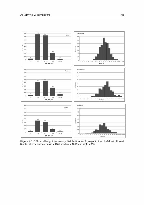
CHAPTER 4: RESULTS 59
Figure 4.1 DBH and height frequency distribution for A. seyal in the Umfakarin Forest Number of observations: dense = 1781, medium = 1235, and slight = 783.
39
770737
212
23
0
100
200
300
400
500
600
700
800
7.5 12.5 17.5 22.5 ≥27.45
DBH class (cm)
Nu
mb
er o
f tr
ees
DenseDense stratum
0
50
100
150
200
250
300
350
0.5 1 1.5 2 2.5 3 3.5 4 4.5 5 5.5 6 6.5 7 7.5 8 8.5 9 9.5 10 10.5 11 11.5
Height (m)
Fre
qu
ency
34
430463
250
58
0
100
200
300
400
500
600
700
800
7.5 12.5 17.5 22.5 ≥27.45
DBH class (cm)
Nu
mb
er o
f tr
ees
MediumMedium stratum
0
50
100
150
200
250
300
350
0.5 1 1.5 2 2.5 3 3.5 4 4.5 5 5.5 6 6.5 7 7.5 8 8.5 9 9.5 10 10.5 11 11.5
Height (m)
Fre
qu
ency
22
349
310
85
17
0
100
200
300
400
500
600
700
800
7.5 12.5 17.5 22.5 ≥27.45
DBH class (cm)
Nu
mb
er o
f tr
ees
Slight
Slight stratum
0
50
100
150
200
250
300
350
0.5 1.0 1.5 2.0 2.5 3.0 3.5 4.0 4.5 5.0 5.5 6.0 6.5 7.0 7.5 8.0 8.5 9.0 9.5 10.0 10.5 11.0 11.5
Height (m)
Fre
qu
ency

CHAPTER 4: RESULTS 60
Figure 4.2 Observed data and the lines of best fit (evaluated height functions) for A. seyal
Table 4.3 Models evaluated for the height curve of A. seyal natural stands in the Umfakarin Forest, South Kordofan, Sudan. Function Function
0a 1a 2a R² AIC
Parabolic 2210 ** dadaah ++= 4.908 0.216 -0.002 0.238 486.36
Petterson
2
10 *3.1
⎟⎟
⎠
⎞
⎜⎜
⎝
⎛
++=
daad
h0.961 0.328 0.239 483.68
Prodan )**/(3.1 2210
2 dadaadh +++= -1.267 0.977 0.095 0.240 483.26
Michailow )/(0
1*3.1 daeah += 8.917 -4.714 0.237 485.94
Hendrickson daah log*10 += 1.762 5.096 0.242 479.00
Van Laar )//( 2210 dadaaeh ++= 2.399 -6.125 13.654 0.240 484.32
Where: h = total height (m); d = diameter at breast height (DBH, in cm); log = natural logarithm; e = base of natural logarithm (≈ 2.7183); a0, a1 and a2 are parameters to be estimated by nonlinear regression; and R² = coefficient of determination. Observations (n = 1235) based on data from
medium stratum.

CHAPTER 4: RESULTS 61
Figure 4.3 illustrates the Michailow height curves for each different stratum in
combination with other observed data. For each stratum, the data points appear to
be randomly scattered, or not around the line of best fit, which indicates a low
correlation between height and diameter. Parameters estimated by the Michailow
height function for the three strata are presented in Table 4.4. R² values ranged from
0.193 in dense stratum to 0.240 in slight stratum. Thus, R² value decreases with an
increase in the number of trees per unit area. Results of statistical test revealed that
the slopes of the height curves in different stand densities are not significantly
different (using the conventional significant level, i.e., α = 0.05). Because the slopes
for the curves in the three strata do not significantly differ, a combined height curve
(R² = 0.227) was produced and included (Figure 4.3, bottom right). The maximum
height (asymptote = 10.2 m) is reached by trees in medium stratum. Trees in dense
and slight strata reach a maximum height of 9.3 and 9.4 m, respectively.
Figure 4.3 Observed data and the line of best fit (Michailow height curve) of A. seyal
0
2
4
6
8
10
12
14
0 5 10 15 20 25 30 35 40
DBH (cm)
Hei
gh
t (m
)
Observed Michailow function
Dense stratum
0
2
4
6
8
10
12
14
0 5 10 15 20 25 30 35 40
DBH (cm)
Hei
gh
t (m
)
Observed Michailow function
Medium stratum
0
2
4
6
8
10
12
14
0 5 10 15 20 25 30 35 40
DBH (cm)
Hei
gh
t (m
)
Observed Michailow function
Slight stratum
0
2
4
6
8
10
12
14
0 5 10 15 20 25 30 35 40
DBH (cm)
Hei
ght
(m)
Dense Medium Slight Combined curve
R² = 0.193R² = 0.237R² = 0.240R² = 0.227

CHAPTER 4: RESULTS 62
Table 4.4 Summary of estimated parameters of the Michailow function used for A seyal height estimation in different strata, Umfakarin Forest, South Kordofan, Sudan.
Stratum n a0 a1 R² Asymptote
Dense 1781 8.039 (0.125) -3.857 (0.193) 0.193 9.3
Medium 1235 8.917 (0.166) -4.714 (0.250) 0.237 10.2
Slight 783 8.102 (0.214) -5.072 (0.328) 0.240 9.4
a0 and a1 are parameters to be estimated by non-linear regression; in parenthesis is the standard error of parameter; n = number of individual trees; R
2 is coefficient of determination.
4.1.2 Volume functions
Figure 4.4 depicts the volume curves, which are applied to estimate the standing
volume of A. seyal, together with observed data for different stand densities. The
data points for all strata are scattered around the line of best fit, up to around 20 cm
DBH. The resulting pattern indicates the dependence of volume on DBH and height.
It is worth mentioning that the height used for the volume function is the estimated
height, for example the height derived from the height curve. Table 4.5 presents the
parameters uncovered by the volume function. The coefficient of determination
ranged from 0.906 in slight stratum to 0.928 in medium stratum. Results of a
statistical test showed that slopes of the three volume curves are not significantly (α =
0.05) different from each other. Consequently, a combined volume curved was
derived.
4.1.3 Relationship between DBH and crown radius
Figure 4.5 depicts the observed data and the fitted curves resulting from the
relationship between DBH and the crown radius (CR). Statistical analysis revealed no
significant difference (p < 0.000) between the observed means of crown radius (2.65,
2.65 and 2.68 m) in dense, medium and slight stands. Table 4.6 provides a summary
of nonlinear regression parameters for crown radius (CR, in m) in relation with DBH
of A. seyal in different strata. The distribution of data points, in all strata, appears to
be randomly scattered, which expresses the poor relationship between CR and DBH.
The slopes of the three fitted regression lines were statistically tested and revealed to
have no significant difference (α = 0.05) from each other. Therefore, a combined
curve was produced. The relationship between CR and DBH at slight stratum
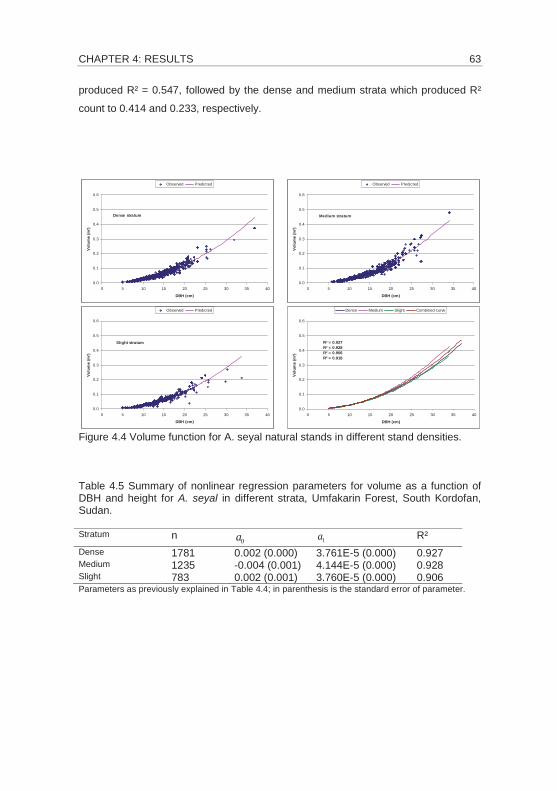
CHAPTER 4: RESULTS 63
produced R² = 0.547, followed by the dense and medium strata which produced R²
count to 0.414 and 0.233, respectively.
Figure 4.4 Volume function for A. seyal natural stands in different stand densities.
Table 4.5 Summary of nonlinear regression parameters for volume as a function of DBH and height for A. seyal in different strata, Umfakarin Forest, South Kordofan, Sudan.
Stratum n 0a 1a R²
Dense 1781 0.002 (0.000) 3.761E-5 (0.000) 0.927 Medium 1235 -0.004 (0.001) 4.144E-5 (0.000) 0.928 Slight 783 0.002 (0.001) 3.760E-5 (0.000) 0.906 Parameters as previously explained in Table 4.4; in parenthesis is the standard error of parameter.
0.0
0.1
0.2
0.3
0.4
0.5
0.6
0 5 10 15 20 25 30 35 40
DBH (cm)
Vo
lum
e (m
³)
Observed Predicted
Dense stratum
0.0
0.1
0.2
0.3
0.4
0.5
0.6
0 5 10 15 20 25 30 35 40
DBH (cm)V
olu
me
(m³)
Observed Predicted
Medium stratum
0.0
0.1
0.2
0.3
0.4
0.5
0.6
0 5 10 15 20 25 30 35 40
DBH (cm)
Vo
lum
e (m
³)
Observed Predicted
Slight stratum
0.0
0.1
0.2
0.3
0.4
0.5
0.6
0 5 10 15 20 25 30 35 40
DBH (cm)
Vo
lum
e (m
³)
Dense Medium Slight Combined curve
R² = 0.927R² = 0.928R² = 0.906R² = 0.918

CHAPTER 4: RESULTS 64
Figure 4.5 Diameter at breast height (DBH) in relation to crown radius (CR) of A. seyal for different stand densities, Umfakarin Forest, South Kordofan, Sudan.
Table 4.6 Summary of nonlinear regression parameters for crown radius (CR, in m) in relation to DBH of A. seyal in different strata, Umfakarin Forest, South Kordofan, Sudan.
Stratum n 0a 1a R²
Dense 1781 -1.840 (0.127) 1.762 (0.050) 0.414 Medium 1189 -3.202 (0.303) 2.225 (0.115) 0.233 Slight 783 -2.588 (0.173) 2.082 (0.068) 0.547
Parameters as previously explained in Table 4.4; in parenthesis is standard error of parameter.
0
1
2
3
4
5
6
7
0 5 10 15 20 25 30 35 40
DBH (cm)
CR
(m
)Observed Predicted
Dense stratum
0
1
2
3
4
5
6
7
0 5 10 15 20 25 30 35 40
DBH (cm)
CR
(m
)
Observed Predicted
Medium stratum
0
1
2
3
4
5
6
7
0 5 10 15 20 25 30 35 40
DBH (cm)
CR
(m
)
Observed Predicted
Slight stratum
0
1
2
3
4
5
6
7
0 5 10 15 20 25 30 35 40
DBH (cm)
CR
(m
)
Dense Medium Slight Combined curve
R² = 0.414R² = 0.233R² = 0.547R² = 0.477

CHAPTER 4: RESULTS 65
4.2 Single tree values
4.2.1 Competition indices (CI) and tree dimensions
4.2.1.1 Frequency distribution of CI-values
Frequency distribution was conducted for three select indices in different stand
densities, including CI_Hegyi and CI_Hegyi_2 which represent distance-dependent
competition indices, and CI_C66 which represents the distance-independent index.
The frequency distribution of the selected indices revealed an irregular distribution
form, as illustrated in Figure 4.6. The pattern of distribution for distance-dependent
index values (at an interval of 0.5) appears to be similar. A normality test was used to
investigate whether the values of these indices are normally distributed or not (Table
4.7). The results illustrate that the values are not normally distributed.
Table 4.7 Results of normality test of selected competition indices
Stratum Index Mean Median SD Min. Max. Skewness Shapiro-Wilk
Statistic P-value
Hegyi 1.56 1.42 0.92 0.11 6.93 1.55 0.91 0.000
Dense C66 148.31 142.33 87.47 0.00 380.68 0.57 0.96 0.000
Hegyi_2 1.83 1.37 1.50 0.05 8.55 1.53 0.86 0.000
Hegyi 1.07 0.92 0.65 0.00 3.44 0.83 0.94 0.000
Medium C66 142.18 114.42 280.42 0.00 3600.0 11.93 0.17 0.000
Hegyi_2 1.35 0.88 1.17 0.00 6.41 1.49 0.84 0.000
Hegyi 0.60 0.51 0.47 0.00 2.19 0.76 0.94 0.000
Slight C66 54.96 37.84 52.72 0.00 279.03 1.44 0.87 0.000
Hegyi_2 0.66 0.47 0.64 0.00 3.26 1.27 0.87 0.000
Number of observations per stratum (dense = 158; medium = 160; slight = 164); SD = standard
deviation
4.2.1.2 Partial correlations
Figure 4.7 illustrates the results of significant partial correlations between various
competition indices (CI) and tree dimensions. Results of the partial correlation
indicate that most indices, with the exception of CI_PRETZSCH, CI_BD_KV and
CI_C66, show a clear and negative significant correlation with DBH in the three
different strata. The maximum negative partial correlation coefficient, (-0.70), was
obtained by CI_HEGYI_2 in dense stratum. The Pretzsch index revealed a negative
correlation for height in dense and slight strata. Other indices, with the exception of
CI_BD_KV and CI_VKF, exhibited a positive correlation with height. Crown diameter
revealed a negative partial correlation with all indices except CI_BAL which showed
no correlation.

CH
AP
TE
R 4
: R
ES
ULT
S
Fig
ure
4.6
Fre
qu
ency d
istr
ibutio
n o
f th
e s
e
66
lecte
d c
om
petition ind
ex v
alu
es f
or
Acacia
seyal
C66
ind
ex, d
ense
str
atu
m
0
10
20
30
40
50
60
70
80
050
100
150
200
250
300
350
400
450
Co
mp
eti
tio
n i
nd
ex
Frequency
0
10
20
30
40
50
60
70
80
00
.51
1.5
Frequency
C66
ind
ex, m
ediu
m s
trat
um
0
10
20
30
40
50
60
70
80
050
100
150
200
250
300
350
400
450
Co
mp
eti
tio
n i
nd
ex
Frequency0
10
20
30
40
50
60
70
80
00
.51
1.5
Frequency
C66
ind
ex, s
ligh
t str
atu
m
0
10
20
30
40
50
60
70
80
050
100
150
200
250
300
350
400
450
Co
mp
eti
tio
n i
nd
ex
Frequency
0
10
20
30
40
50
60
70
80
00
.51
1.5
Frequency
Heg
yi_2
ind
ex, d
ense
str
atu
m
22
.53
3.5
44
.55
5.5
66.5
77.5
88.5
99
.510
Co
mp
eti
tio
n i
nd
ex
Heg
yi_2
ind
ex, m
ediu
m s
trat
um
22
.53
3.5
44
.55
5.5
66.5
77.5
88.5
99
.510
Co
mp
eti
tio
n i
nd
ex
He
gyi
_2 in
dex
, slig
ht s
trat
um
22
.53
3.5
44
.55
5.5
66.5
77.5
88.5
99
.510
Co
mp
eti
tio
n i
nd
ex
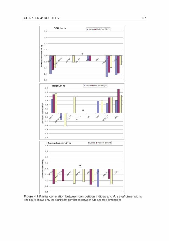
CHAPTER 4: RESULTS 67
Figure 4.7 Partial correlation between competition indices and A. seyal dimensions The figure shows only the significant correlation between CIs and tree dimensions
DBH, in cm
-0.8
-0.6
-0.4
-0.2
0.0
0.2
0.4
0.6
0.8
HEG
YI
PRETZSC
H
BD_K
F
BD_K
VVKF
C66
HEG
YI_
2BAL
CI
Co
rrel
atio
n c
oef
fici
ent
(r)
Dense Medium Slight
Height, in m
-0.6
-0.5
-0.4
-0.3
-0.2
-0.1
0.0
0.1
0.2
0.3
0.4
0.5
0.6
HEG
YI
PRETZSC
H
BD_K
F
BD_K
VVKF
C66
HEG
YI_
2BAL
CI
Co
rrea
ltio
n c
oef
fici
ent
(r)
Dense Medium Slight
Crown diameter , in m
-0.4
-0.3
-0.2
-0.1
0.0
0.1
0.2
0.3
0.4
HEGYI
PRETZSC
H
BD_K
F
BD_K
VVKF
C66
HEGYI_
2BAL
CI
Co
rrel
atio
n c
oef
fici
ent
(r)
Dense Medium Slight
CHAPTER 4: RESULTS 68
4.2.1.3 Selection of an appropriate competition index
The relationship between tree dimensions (DBH, height and crown diameter) and
various competition indices was tested by a logarithmic function. The criterion for
selecting the appropriate index that better relates to the tree dimension in a specific
stratum was based on the coefficient of determination (R²); the higher the value of R²,
the better the index expresses the relationship. Values of R² vary according to tree
dimension, competition index and stand density. Table 4.8 depicts the result of the
association between tree dimensions and competition index values at different stand
densities. In this table, the maximum R² (0.690) was obtained as a result of the
relationship between DBH and the HEGYI_2 index in dense stratum. Another index,
such as the Hegyi index, has also produced a significant relationship (R² = 0.238 to
0.471) with DBH. Tree height on the other hand, revealed a negligible association
with all indices, with the exception of the Pretzsch index (R² = 0.238) in slight
stratum. After further inspection of this table, tree crown diameter revealed no
relationship with all indices meaning that crown diameter is independent to stand
density or competition. Based on the results of this table, Hegyi_2 is the most
important index as it better relates to DBH. Thus, Hegyi_2 index can be considered
an appropriate index for expressing competitive situations using DBH as an
explanatory variable. The selected logarithmic model is able to explain up to 70
percent of the variation. Scatter plots with logarithmic fitted lines, as a result of the
association between DBH and the Hegyi_2 index for the different stand densities,
were produced and are displayed in Figure 4.8. The data points are randomly
scattered and do not lie on the line of best fit in medium and slight strata. However in
dense stratum, the data points are scattered around the line of best fit, with some
scattered points which indicate the presence of outliers. In this figure, the value of the
competition index decreases as the DBH increases and the line of the best fit points
down to the right, indicating a negative relationship between CI and DBH. In general,
CI decreases and approaches zero when DBH exceeds 22 cm in all strata.
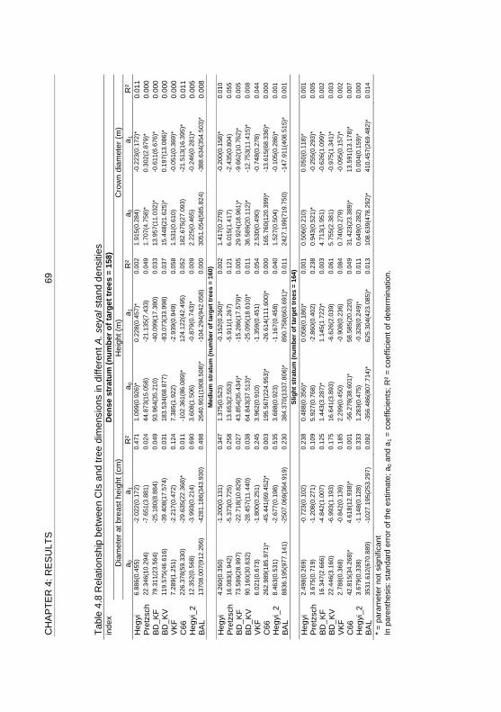
CH
AP
TE
R 4
: R
ES
ULT
S
69
Table
4.8
Rela
tionsh
ip b
etw
ee
n C
Is a
nd t
ree d
imensio
ns in d
iffe
rent
A. seyal sta
nd d
ensitie
s
ind
ex
Den
se s
trat
um
(n
um
ber
of
targ
et t
rees
= 1
58)
Dia
mete
r at
bre
ast he
ight (c
m)
Heig
ht (m
) C
row
n d
iam
ete
r (m
)
a0
a1
R²
a0
a1
R²
a0
a1
R²
Heg
yi
6.8
86(0
.455)
-2.0
22(0
.172)
0.4
71
1.0
99(0
.926)*
0.2
28(0
.457)*
0.0
02
1.9
15(0
.284)
-0.2
23(0
.172)*
0.0
11
Pre
tzsch
22.3
46(1
0.2
94)
-7.6
51(3
.881)
0.0
24
44.8
73(1
5.0
58)
-21.1
35(7
.433)
0.0
49
1.7
07(4
.758)*
0.3
02(2
.879)*
0.0
00
BD
_K
F
79.3
11(2
3.5
64)
-25.1
80(8
.884)
0.0
49
93.9
64(3
5.2
10)
-40.0
99(1
7.3
80)
0.0
33
13.9
57(1
1.0
32)*
-0
.611(6
.676)*
0.0
00
BD
_K
V
119.5
75(4
6.6
16)
-39.4
08(1
7.5
74)
0.0
31
183.5
34(6
8.8
77)
-83.0
73(3
3.9
98)
0.0
37
15.4
48(2
1.6
25)*
0.1
97(1
3.0
86)*
0.0
00
VK
F
7.2
89(1
.251)
-2.2
17(0
.472)
0.1
24
7.3
85(1
.922)
-2.9
39(0
.949)
0.0
58
1.5
31(0
.610)
-0.0
51(0
.369)*
0.0
00
C66
226.3
78(5
9.3
30)
-29.6
35(2
2.3
68)*
0.0
11
-102.3
61(8
6.0
89)*
124.1
22(4
2.4
95)
0.0
52
182.6
75(2
7.0
93)
-21.5
13(1
6.3
95)*
0.0
11
Heg
yi_
2
12.3
52(0
.568)
-3.9
93(0
.214)
0.6
90
3.6
08(1
.506)
-0.8
79(0
.743)*
0.0
09
2.2
25(0
.465)
-0.2
46(0
.281)*
0.0
05
BA
L
13708.0
07(9
12.2
66)
-4281.1
86(3
43.9
30)
0.4
98
2640.9
01(1
908.5
08)*
-1
04.2
94(9
42.0
58)
0.0
00
3051.0
54(5
85.8
24)
-388.6
34(3
54.5
03)*
0.0
08
Med
ium
str
atu
m (
num
ber
of
targ
et t
rees
= 1
60)
Heg
yi
4.2
60(0
.350)
-1.2
00(0
.131)
0.3
47
1.3
75(0
.523)
-0.1
52(0
.260)*
0.0
02
1.4
17(0
.279)
-0.2
00(0
.158)*
0.0
10
Pre
tzsch
16.0
83(1
.942)
-5.3
73(0
.725)
0.2
58
13.6
53(2
.553)
-5.9
11(1
.267)
0.1
21
6.0
15(1
.417)
-2.4
35(0
.804)
0.0
55
BD
_K
F
73.5
89(2
8.9
97)
-22.7
18(1
0.8
29)
0.0
27
43.8
54(3
5.4
34)*
-1
5.2
86(1
7.5
79)*
0.0
05
29.9
24(1
8.9
61)*
-9
.662(1
0.7
62)*
0.0
05
BD
_K
V
90.1
60(3
0.6
32)
-28.4
57(1
1.4
40)
0.0
38
64.8
43(3
7.5
13)*
-2
5.0
95(1
8.6
10)*
0.0
11
36.5
89(2
0.1
12)*
-1
2.7
53(1
1.4
15)*
0.0
08
VK
F
6.0
21(0
.673)
-1.8
00(0
.251)
0.2
45
3.9
62(0
.910)
-1.3
59(0
.451)
0.0
54
2.5
30(0
.490)
-0.7
48(0
.278)
0.0
44
C66
262.9
89(1
85.9
71)*
-4
5.4
41(6
9.4
52)*
0.0
03
195.5
67(2
24.9
53)*
-2
6.6
14(1
11.6
00)*
0.0
00
165.7
60(1
20.3
99)*
-1
3.6
15(6
8.3
36)*
0.0
00
Heg
yi_
2
8.4
63(0
.531)
-2.6
77(0
.198)
0.5
35
3.6
88(0
.923)
-1.1
67(0
.458)
0.0
40
1.5
27(0
.504)
-0.1
05(0
.286)*
0.0
01
BA
L
8836.1
95(9
77.1
41)
-2507.0
69(3
64.9
19)
0.2
30
384.3
70(1
337.8
06)*
890.7
58(6
63.6
91)*
0.0
11
2427.1
99(7
19.7
50)
-147.9
11(4
08.5
15)*
0.0
01
Slig
ht
stra
tum
(nu
mb
er o
f ta
rget
tre
es =
164
)
Heg
yi
2.4
98(0
.269)
-0.7
23(0
.102)
0.2
38
0.4
88(0
.356)*
0.0
58(0
.186)*
0.0
01
0.5
06(0
.210)
0.0
50(0
.118)*
0.0
01
Pre
tzsch
3.6
75(0
.719)
-1.2
08(0
.271)
0.1
09
5.9
27(0
.768)
-2.8
60(0
.402)
0.2
38
0.9
43(0
.521)*
-0
.255(0
.293)*
0.0
05
BD
_K
F
16.3
47(2
.666)
-4.8
42(1
.007)
0.1
25
1.4
43(3
.287)*
1.1
45(1
.722)*
0.0
03
4.7
13(1
.951)
-0.6
26(1
.099)*
0.0
02
BD
_K
V
22.4
46(3
.160)
-6.9
93(1
.193)
0.1
75
16.6
41(3
.893)
-6.6
26(2
.039)
0.0
61
5.7
55(2
.381)
-0.9
75(1
.341)*
0.0
03
VK
F
2.7
88(0
.368)
-0.8
42(0
.139)
0.1
85
2.2
99(0
.450)
-0.9
08(0
.236)
0.0
84
0.7
40(0
.279)
-0.0
95(0
.157)*
0.0
02
C66
42.8
15(3
4.2
68)*
4.6
18(1
2.9
38)*
0.0
01
-56.2
78(3
8.6
01)*
58.5
85(2
0.2
20)
0.0
49
31.4
23(2
3.3
89)*
13.5
91(1
3.1
78)*
0.0
07
Heg
yi_
2
3.6
79(0
.338)
-1.1
48(0
.128)
0.3
33
1.2
83(0
.475)
-0.3
28(0
.249)*
0.0
11
0.6
49(0
.282)
0.0
04(0
.159)*
0.0
00
BA
L
3531.6
12(6
70.8
89)
-1027.1
95(2
53.2
97)
0.0
92
-356.4
86(8
07.7
14)*
625.3
04(4
23.0
85)*
0.0
13
108.6
39(4
78.2
92)*
410.4
57(2
69.4
82)*
0.0
14
* =
para
mete
r not
sig
nific
an
t
In p
are
nth
esis
: sta
ndard
err
or
of th
e e
stim
ate
; a
0 a
nd a
1 =
coe
ffic
ients
; R
² =
co
effic
ient
of
dete
rmin
ation
.

CHAPTER 4: RESULTS 70
Figure 4.8 Acacia seyal and the relationship between DBH and competition index (CI) values (CI_Hegyi_2)
0
1
2
3
4
5
6
7
8
9
0 5 10 15 20 25 30 35 40
DBH (cm)
CI
valu
e
Observed Predicted
Dense
0
1
2
3
4
5
6
7
8
9
0 5 10 15 20 25 30 35 40
DBH (cm)
CI
valu
es
Observed Predicted
Slight
0
1
2
3
4
5
6
7
8
9
0 5 10 15 20 25 30 35 40
DBH (cm)
CI
valu
e
Observed Predicted
Medium
0
1
2
3
4
5
6
7
8
9
0 5 10 15 20 25 30 35 40
DBH (cm)
CI
valu
es
Dense Medium Slight
CI = 12.352-3.993*ln(DBH)CI = 8.463-2.677*ln(DBH)CI = 3.679-1.148*ln(DBH)R² = 0.690R² = 0.535R² = 0.333

CHAPTER 4: RESULTS 71
4.2.2 Production of gum talha from natural stands of A. seyal
A total of 482 individual trees of natural A. seyal, of three different stand densities,
were selected and exposed to tapping techniques by local tapping tools on three
tapping dates. Average gum yield and the number of individual trees per each
tapping treatment are shown in Table 4.9. Trees tapped by sonki (n= 16) on first of
October at medium stratum have the highest gum yield, with a value of about 56
g/tree/season. The minimum gum yield, 2 g/tree/season, was obtained on 15 October
by 18 untapped trees in slight stratum.
Gum talha yields are classified into six yield classes (g) namely, ≤ 50, 51-100, 101-
150, 151-200, 201-250 and ≥ 251 g. In each yield class, the number of trees in
addition to the total and average gum talha yield (g) in different stand densities were
obtained and summarized in Table 4.10. The maximum total gum yield (1076.07 g)
was obtained in the lowest yield class (≤ 50 g) by 84 observations in dense stratum.
Upper yield classes are characterized by few or absence of trees. Irrespective of
tapping date and tool of tapping, the average gum yield (g) of a tree per season and
gum production (kg/hectare/season) were also obtained for the different stand
densities. On average, trees in slight stratum produced a higher amount of gum
(20.58 g/tree/season) than those of the other strata. Gum talha production ranges
between 3.59 to 4.78 kg/ha. In all strata, a high number of trees (between 41-53
percent) in the lowest gum yield class (≤ 50 g) were detected. The number of trees in
the second yield class upwards represents less than 5 percent of the selected trees
in dense stratum. In medium and slight strata, the number of trees in the same yield
classes represents about 6 and 13 percent, respectively. The high yielding trees for
example classes 151-200 and upwards, constitute about only 2 percent of the total
target trees (482). Non-yielding trees constitute about 43, 53 and 45 percent of the
selected trees in dense, medium and slight stratum, respectively.
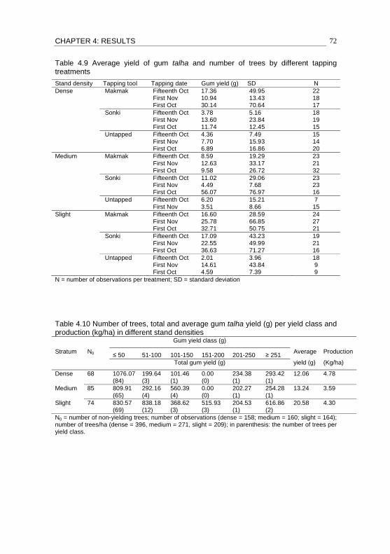
CHAPTER 4: RESULTS 72
Table 4.9 Average yield of gum talha and number of trees by different tapping treatments
Stand density Tapping tool Tapping date Gum yield (g) SD N
Dense Makmak Fifteenth Oct 17.36 49.95 22 First Nov 10.94 13.43 18 First Oct 30.14 70.64 17
Sonki Fifteenth Oct 3.78 5.16 18 First Nov 13.60 23.84 19 First Oct 11.74 12.45 15
Untapped Fifteenth Oct 4.36 7.49 15 First Nov 7.70 15.93 14 First Oct 6.89 16.86 20
Medium Makmak Fifteenth Oct 8.59 19.29 23
First Nov 12.63 33.17 21 First Oct 9.58 26.72 32
Sonki Fifteenth Oct 11.02 29.06 23 First Nov 4.49 7.68 23 First Oct 56.07 76.97 16
Untapped Fifteenth Oct 6.20 15.21 7
First Nov 3.51 8.66 15
Slight Makmak Fifteenth Oct 16.60 28.59 24 First Nov 25.78 66.85 27 First Oct 32.71 50.75 21
Sonki Fifteenth Oct 17.09 43.23 19 First Nov 22.55 49.99 21 First Oct 36.63 71.27 16
Untapped Fifteenth Oct 2.01 3.96 18 First Nov 14.61 43.84 9 First Oct 4.59 7.39 9
N = number of observations per treatment; SD = standard deviation
Table 4.10 Number of trees, total and average gum talha yield (g) per yield class and production (kg/ha) in different stand densities Gum yield class (g)
Stratum N0≤ 50 51-100 101-150 151-200 201-250 ≥ 251
Average Production
Total gum yield (g) yield (g) (Kg/ha)
Dense 68 1076.07(84)
199.64 (3)
101.46 (1)
0.00 (0)
234.38 (1)
293.42 (1)
12.06 4.78
Medium 85 809.91 (65)
292.16 (4)
560.39 (4)
0.00 (0)
202.27 (1)
254.28 (1)
13.24 3.59
Slight 74 830.57 (69)
838.18 (12)
368.62 (3)
515.93 (3)
204.53 (1)
616.86 (2)
20.58 4.30
N0 = number of non-yielding trees; number of observations (dense = 158; medium = 160; slight = 164); number of trees/ha (dense = 396, medium = 271, slight = 209); in parenthesis: the number of trees per yield class.

CHAPTER 4: RESULTS 73
4.2.3 Factors affecting gum yield
4.2.3.1 Gum yield and tree size (DBH)
Regardless of the gum tapping treatments, the relationship between gum yield and
DBH for the different three stand densities was tested. Observed values and the
modelled ones-smooth lines are graphically presented in Figure 4.9. The data dots
are randomly distributed, indicating a high-level of variability for yields in all strata.
The following linear regression model (Equation 36) based on the same figure could
be used to predict the yield of gum talha in medium stratum; where Y is the predicted
gum yield (g) per tree and d is the tree diameter (DBH, in cm). Generally, as gum
yield increases, DBH also increases. Dense stratum, however, produce a curved
space below the curves of medium and slight strata. The maximum R² value (0.146)
was obtained in medium stand density. This means that the model is able to explain
a small proportion (only 15%) of gum yield variation.
� � 3.562 � 28.061 ........................................................................................... (36)
Parameters are described in the text.
Figure 4.9 Gum talha yield in relation to tree diameter for different stand densities Number of observations per stratum (dense = 90, medium = 75 and slight = 90)
0
50
100
150
200
250
300
350
400
0 5 10 15 20 25 30 35 40
DBH (cm)
Gum
yie
ld (
g)
Observed_dense Predicted_dense Observed_medium Predicted_medium
Observed_slight Predicted_slight
Y = 6.386+0.983*DBHY = 3.562*DBH-28.061Y = 27.426+0.656*DBHR² = 0.010R² = 0.146R² = 0.003

CHAPTER 4: RESULTS 74
4.2.3.2 Determining factors influencing gum yield using regression tree
To examine factors determining gum talha yield, the regression tree package was
used and was applied to predict the mean value of gum yield obtained from A. seyal
trees using different tapping treatments. Gum yield, a measurable response variable,
can be expressed as a function of several explanatory-measurable and categorical-
variables. These explanatory variables include: stand density (dense, medium and
slight), tapping tool (makmak, sonki and untapped trees) and the date of tapping (1st
October, 15th October and 1st November) in addition to DBH and competition index
(CI). The regression tree model is shown in Figure 4.10. This figure illustrates that
the model contains of 6 terminal nodes (or leaves, i.e. 4, 6, 7, 10, 22 and 23). DBH,
tapping tool, date of tapping and CI contribute to the construction of the tree. DBH is
the most important explanatory variable that influences gum yield. The model splits
the original data set into two partitions, below and above the DBH threshold value
(23.95 cm), which are not evenly distributed. The data set below the threshold
includes 97% of the total observations, whereas the set above the threshold reflects
only 3% of the observations (see right-hand branch of the Figure 4.10). The model
starts with the root node (1) which contains the entire data set (n = 482). The model
indicates that the overall mean value of gum is 15.35 g. The predicted mean values
of gum yield and number of cases (n) for each terminal node are provided in the
same figure. The intermediate and terminal nodes´ number is depicted in
parentheses. In the left-hand branch and in the terminal node (4), the minimum gum
yield value (5.87 g) is given by 105 untapped trees when DBH is less than the
threshold (23.95 cm). In node 7, located in the right-hand branch, the maximum gum
yield (124.70 g) is only obtained by 8 trees with DBH larger than the threshold when
CI is greater than 0.125. Further details regarding the results of regression tree
analysis for predicting gum talha yield are shown in Appendix 4. Node number,
variables used at each split and split criterion, number of observations, the deviance
associated with split and mean value of gum yield (g) are obtained and summarized
in the same appendix.

CHAPTER 4: RESULTS 75
Figure 4.10 Regression tree model for predicting yield of gum talhaMeans of gum yield are shown in the terminal nodes (4, 6, 7, 10, 22 and 23); in parentheses are node number; n is the number of observation per node; CI = Hegyi_2 competition index; tool (a: makmak, b: sonki, c: untapped trees); date (a: 15
th October, b: 1
st November, c: 1
st October).
4.2.3.3 Determining factors that influence gum yield using GLM
The results of the regression analysis under a general linear model
(GLM)/UNIVARIATE showed that at least one treatment is different. To explore the
differences in gum yield among significant categorical variables in each stratum,
post-hoc tests (or post-hoc comparison tests) following ANOVA and based on
Scheffé test were carried out. The results of the ANOVA showed that only the date of
tapping is significant for medium stratum. Tapping tool is not significant in all strata
(Appendix 5). The Tests of Between-Subject Effects table (Appendix 6), shows the
results of GLM univariate in which gum talha yield is estimated per each stratum by
the fixed factors (tapping date and tool of tapping) in addition to DBH and CI as
covariates. The results show that the only significant (p = 0.000) overall model is in
medium stratum and the effect size is partial eta squared (analogous to R2 = 0.304),
meaning that the model explains 30.4% of the variance in gum talha yield. The
overall models in dense and medium strata are not significant. Table 4.11 provides

CHAPTER 4: RESULTS 76
information about whether the means of gum yield for different tapping dates are
significantly (α = 0.05) different from each other. In this table, the results of the post-
hoc test indicate that the significance (p < 0.021) detected stemmed from a difference
between just two groups of dates; the first of October vs. the first of November. The
other comparisons were found to be insignificant. More details about the differences
in gum yield are presented in the table of the homogenous subset (Table 4.12). As
illustrated by this table, the outputs of Scheffé test produces gum averages either in
one subset or two subsets for each group. Averages within the same subset are not
significantly different from each other (α = 0.05). For example, in the case of one
subset in dense and slight strata, there is no significant difference in gum yield
between the different tapping dates. However, for medium stratum, there are two
subsets. This means that, in the first subset, there is no difference (p = 0.943) in gum
yield between the fifteen of October and the first of November. In the second subset,
there is also no difference between first and fifteen of October. However, gum yield is
different (p = 0.050) between the first of October and the first of November.
Table 4.11 Post-hoc-test, following ANOVA, based on Scheffé test for testing the difference in gum talha yield
Stratum Date (X) Date (Y) Gum mean difference (X-Y)
SE Sig. 95% Confidence limit
Lower Upper
Dense
First of October
Fifteen of October
6.516 6.291 0.586 -9.040 22.073
First of November
4.848 6.410 0.752 -11.002 20.698
Fifteen of October
First of November
-1.668 6.323 0.966 -17.303 13.966
First of
October
Fifteen of
October
15.748 6.535 0.058 -0.407 31.902
Medium First of November
17.939* 6.375 0.021 2.180 33.698
Fifteen of October
First of November
2.191 6.207 0.940 -13.152 17.535
First of October
Fifteen of October
16.122 9.442 0.236 -7.215 39.459
Slight First of
November
5.747 9.583 0.836 -17.939 29.433
Fifteen of October
First of November
-10.375 8.907 0.509 -32.391 11.640
*. The mean difference is significant at the 0.05 level X and Y are specified dates; SE is the standard error of the mean
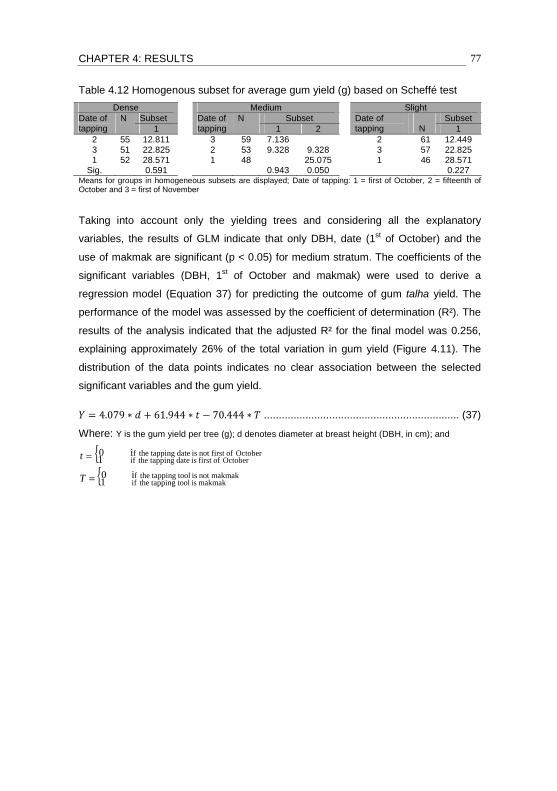
CHAPTER 4: RESULTS 77
Table 4.12 Homogenous subset for average gum yield (g) based on Scheffé test
Dense Medium Slight
Date of
tapping
N Subset Date of
tapping
N Subset Date of
tapping N
Subset
1 1 2 1
2 55 12.811 3 59 7.136 2 61 12.449
3 51 22.825 2 53 9.328 9.328 3 57 22.825 1 52 28.571 1 48 25.075 1 46 28.571
Sig. 0.591 0.943 0.050 0.227 Means for groups in homogeneous subsets are displayed; Date of tapping: 1 = first of October, 2 = fifteenth of October and 3 = first of November
Taking into account only the yielding trees and considering all the explanatory
variables, the results of GLM indicate that only DBH, date (1st of October) and the
use of makmak are significant (p < 0.05) for medium stratum. The coefficients of the
significant variables (DBH, 1st of October and makmak) were used to derive a
regression model (Equation 37) for predicting the outcome of gum talha yield. The
performance of the model was assessed by the coefficient of determination (R²). The
results of the analysis indicated that the adjusted R² for the final model was 0.256,
explaining approximately 26% of the total variation in gum yield (Figure 4.11). The
distribution of the data points indicates no clear association between the selected
significant variables and the gum yield.
� � 4.079 � 61.944 � � 70.444 � .................................................................. (37)
Where: Y is the gum yield per tree (g); d denotes diameter at breast height (DBH, in cm); and
{ October offirst is date tapping theifOctober offirst not is date tapping thef
1i0=t
{ makmak is tool tapping theifmakmaknot is tool tapping thef
1i0=T

CHAPTER 4: RESULTS 78
Figure 4.11 Observed and predicted gum yield (g) of Acacia seyal at medium stratum
Number of observations (only yielding trees) = 75; d = DBH (cm); t = time of tapping (1st of October); T
= tapping tool (makmak)
4.2.3.4 Determining factors affecting gum yield using logistic regression
The classification table (Table 4.13) displays the correctly (predicted), incorrectly (not
predicted) and overall predictions of the binary logistic model results. The model was
used to classify both yielding and non-yielding trees. For instance, the percent of
correctly classified yielding trees was calculated by dividing the number of correctly-
classified cases by the number of correctly and incorrectly predicted observations.
However, the overall percentage correct was obtained by adding the total correctly
predicted yielding trees with the correctly predicted non-yielding trees and then
dividing the total of the two by the total observations for both yielding and non-
yielding trees. In dense stratum, the model correctly classified 80.2% of trees as
yielding trees and 46.3% of the non-yielding trees. Similarly, in the medium stratum
the model correctly identified 54.7% of the yielding trees and 70.6% of the non-
yielding trees, whereas 74.4% and 54.1% were correctly classified, respectively, for
yielding and non-yielding trees in the slight stratum. The classification table shows
that the model’s overall predictions (total predictive efficiency) account for 65.8, 63.1
and 65.2% for dense, medium and slight strata, respectively.
The results of the logistic regression analysis and the variables to be used in the
model are presented in Table 4.14. The significance of each variable is measured
0
50
100
150
200
250
300
0 5 10 15 20 25 30 35 40
Tree diameter (DBH, cm)
Gu
m y
ield
(g
)
Observed yield Predicted yield
Y = 4.079*d+61.944*t-70.444*t*TR² = 0.256
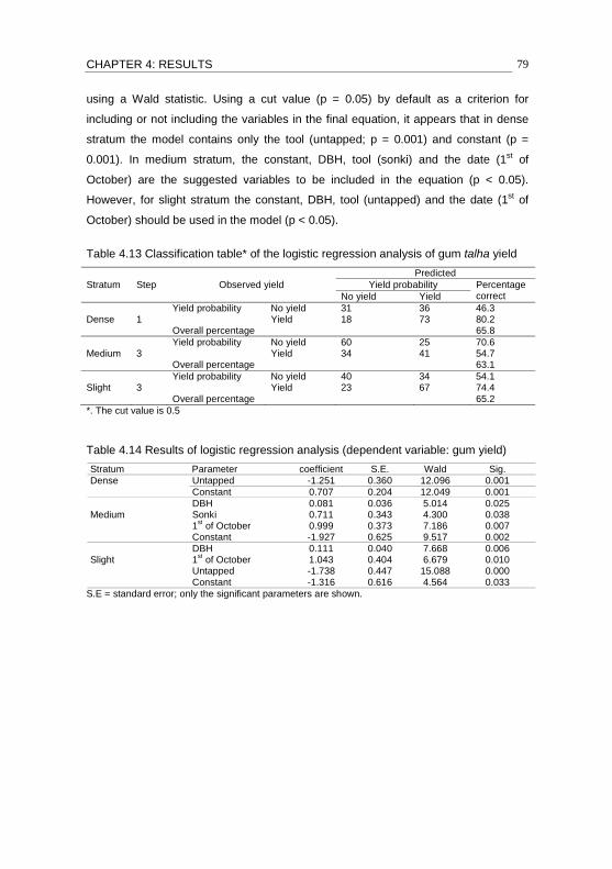
CHAPTER 4: RESULTS 79
using a Wald statistic. Using a cut value (p = 0.05) by default as a criterion for
including or not including the variables in the final equation, it appears that in dense
stratum the model contains only the tool (untapped; p = 0.001) and constant (p =
0.001). In medium stratum, the constant, DBH, tool (sonki) and the date (1st of
October) are the suggested variables to be included in the equation (p < 0.05).
However, for slight stratum the constant, DBH, tool (untapped) and the date (1st of
October) should be used in the model (p < 0.05).
Table 4.13 Classification table* of the logistic regression analysis of gum talha yield
Predicted
Stratum Step Observed yield Yield probability Percentage correct No yield Yield
Yield probability No yield 31 36 46.3 Dense 1 Yield 18 73 80.2 Overall percentage 65.8
Yield probability No yield 60 25 70.6 Medium 3 Yield 34 41 54.7 Overall percentage 63.1
Yield probability No yield 40 34 54.1 Slight 3 Yield 23 67 74.4
Overall percentage 65.2
*. The cut value is 0.5
Table 4.14 Results of logistic regression analysis (dependent variable: gum yield)
Stratum Parameter coefficient S.E. Wald Sig.
Dense Untapped -1.251 0.360 12.096 0.001
Constant 0.707 0.204 12.049 0.001
Medium DBH 0.081 0.036 5.014 0.025 Sonki 0.711 0.343 4.300 0.038 1
st of October 0.999 0.373 7.186 0.007
Constant -1.927 0.625 9.517 0.002
Slight DBH 0.111 0.040 7.668 0.006 1
st of October 1.043 0.404 6.679 0.010
Untapped -1.738 0.447 15.088 0.000
Constant -1.316 0.616 4.564 0.033
S.E = standard error; only the significant parameters are shown.
CHAPTER 5: DISCUSSION 80
5 DISCUSSION
The following chapter presents the discussion on the results revealed in the present
study. There are three sections included in this chapter. The first one deals with
stand structure, composition and modeling height and volume functions of A. seyal.
The second section discusses the competition among individual trees of A. seyal in
natural stands. The third section focuses on the production of gum talha, factors
affecting the production and models for gum talha yield.
5.1 Stand characteristics
Stand characteristics, such as composition, structure, basal area, and volume, are
common attributes assigned to entire stands based on plot measurements.
5.1.1 Forest composition and structure
As previously mentioned three stands densities, based on the number of trees per
unit area, of A. seyal in the Umfakarin Natural Forest Reserve were distinguished,
namely dense, medium and slight strata. Important features of these stands can be
described as mono-species, single-layered, and naturally regenerated. Additionally,
there have been no silvicultural treatments or felling operations in the forest, with the
exception of illegal felling in some parts of the forest by local people who live
adjacent to the reserve. The stands are typical for the Garri forest in Blue Nile, Sudan
which was described by Vink (1990a) as “A. seyal formation of 10-20 years old, of
natural origin, pure, no understory, no natural regeneration and the site is being
grazed by villages´ livestock”. A. seyal of different densities dominate the forest,
nevertheless, other trees and/or shrubs are also found, such as A. mellifera,
Balanites aegyptiaca, A. polycantha, A. senegal, A. nilotica, A. sieberana, Cordia
Africana, Boscia senegalensis, and Dichrystachst sinaria.
Stand structure is the distribution of species and tree sizes in a forest area (Husch et
al., 1993). Distribution of diameters and the heights of trees, in a specific stand, is a
good criterion not only for describing the horizontal and vertical structure of the stand
but to also provide basic information for forest resource management. Moreover,
trees of different diameters may be used for different purposes and have different
values per cubic meter of wood (Philip, 1994). In the present study, the height
CHAPTER 5: DISCUSSION 81
frequency distribution is approximately normal in the dense stratum, yet it is irregular
in the other strata. On the other hand, the diameter is approximately normally
distributed and the pattern of distribution appears to be similar in the three stand
densities. The number of individuals is higher in the second and third diameter
classes. In contrast, there are few stems in the small (DBH = 7.5 cm) and large
diameter classes (DBH = 22.5+ cm). Egadu et al. (2006), in their study of the
population of acacia tree species producing gum Arabic in Karamoja, Uganda,
revealed a higher number of stems of A. seyal in smaller diameter classes indicating
good regeneration. Conversely, in this study few stems were detected in the smaller
diameter class indicating poor natural regeneration. The lower number of stems in
the 22.5 diameter class and upwards could be attributed to illegal felling in some
parts of the forest. Despite protection measures against illegal felling, temporary
informal tracks were created inside the forest by loggers to facilitate wood extraction
(diameters 22.5+ cm) for different purposes.
5.1.2 Natural regeneration
A. seyal is a light demander; it is a rapidly growing species and its small seedlings
colonize open sites quickly (Figure 3.6). The aggregation of A. seyal natural
generation (4867 seedlings per hectare) demonstrates that the species, in its natural
habitats, successfully compete with other vegetation types (woody and/or grass
species). The species grows fast and mature trees tend to close the canopy which
may lessen the growth efficiency of other vegetation. In the present investigation, the
number of natural regeneration per unit area in all strata is quite poor (maximum 50
seedlings per hectare), which is not promising. The unsatisfactory natural
regeneration may be due to the seedlings mortality caused by frequent forest
disturbances such as continuous grazing and fires. These disturbance factors are
very common in the area of investigation. The situation exemplifies the absence of
tending operations to assist natural regeneration.
5.1.3 Height-diameter relationship
Height and diameter are the most frequent measurements made by foresters in order
to estimate growth and/or the yield of trees in forest stands. El-Juhany and Aref
(2001) indicated that, under uniform site conditions, trees of the same age grow in
height at roughly the same rate but not necessarily the same in diameter. They

CHAPTER 5: DISCUSSION 82
further noted that, in uniform site conditions, trees of the same diameter do not
necessarily having the same height. However, in tropical natural forest stands, it is
difficult to estimate tree age, hence trees growing under the same site conditions do
not necessarily grow in height at the same rate. Variation in heights and diameters
may be due to competition and difference in tree age.
One of the most important elements of forest structure is the relationship between
tree diameters and heights (Zucchini et al., 2001). A stand height curve is a
mathematical or graphical representation that describes the dependency of tree
height on diameter. The height curve can be used to predict individual tree height
when only DBH is measured. Moreover, the predicted height can be used together
with DBH to derive single tree volume and/or to produce volume table (2-way volume
table) of a forest stands. In this investigation, six height functions were proposed for
testing the height-diameter relationship of A. seyal trees in natural stands. The
criteria adopted for examining the performance of the height curves were the R²
value, AIC, curve shape and asymptote. However, Laar and Akça (2007) and
Yuancai and Parresol (2001) suggested that the fit curve should satisfy specific
criteria. These criteria are monotonic increment (increasing height with increasing
diameter), inflection point (the point(s) where the curve change its direction) and
asymptote (when the diameter goes to infinity). In reality, height increases with
increasing diameter but not absolute, it should increase to a certain limit. Based on
these criteria Michailow height function was selected because in addition to plausible
curve shape, about 23% of the total height variability is explained. Nevertheless, the
Michailow height curve was compared to parabolic function which was used by
Elsiddig (2003b) for estimating height of A. seyal in eastern Sudan (Figure 5.1). The
later function produces R² value greater than that of Michailow but does not satisfy
the criteria which proposed by the authors (Laar and Akça, 2007; Yuancai and
Parresol, 2001). Both models revealed biologically logical trend up to 30 cm DBH,
then height by parabolic decreases with increasing DBH which is not acceptable from
biological view point. The Michailow height function also satisfies the asymptote
which corresponds to the maximum height (10.2 m) when DBH goes to infinity. The
parabolic function does not satisfy this criterion. Based on these findings, Michailow
height function (Equation 38) was used for predicting height of A. seyal trees in
Umfakarin natural forest, Sudan and in other areas of similar climatic conditions.

CHAPTER 5: DISCUSSION 83
� � 1.3 � 8.486 ���
�.���
�
�
………………………………………………….……………. (38)
Parameter as previously explained.
Figure 5.1 Michailow and parabolic height curves used for predicting height of A. seyal trees in Umfakarin natural forest, Sudan
5.1.4 Single tree and stand volume functions
In forest stands, yield of wood is usually measured in terms of standing volume of
trees which is mostly dependent on site quality and silvicultural management. A.
seyal in Sudan is considered as one of the original sources for firewood and charcoal
since the species is growing rapidly and requiring minimum management (Wickens et
al., 1995). Findings related to the standing volume in the present investigation, are
similar to that estimates obtained by El Dool (1988) at Khor Donya forest (~ 700 mm
mean annual rainfall) in Blue Nile province, Sudan, who revealed to an average
volume of 20.5 m³/ha, 5.2 m²/ha BA and 373 stem/ha of A. seyal (10-20 years old).
The similarity of these findings is expecting elsewhere in Sudan because A. seyal is
growing naturally in specific zone of similar climatic conditions.
Mathematical models for estimating timber yields are usually developed by fitting a
suitable equation to observed data (Gadow and Hui, 1999). In this investigation,
volume of A. seyal trees was estimated using the volume function of two-entries (i.e.
0
1
2
3
4
5
6
7
8
9
10
0 5 10 15 20 25 30 35 40
DBH (cm)
Hei
gh
t (m
)
Michailow Parabolic
R² = 0.227R² = 0.233
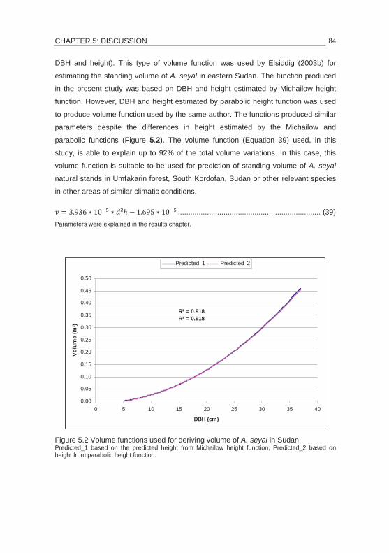
CHAPTER 5: DISCUSSION 84
DBH and height). This type of volume function was used by Elsiddig (2003b) for
estimating the standing volume of A. seyal in eastern Sudan. The function produced
in the present study was based on DBH and height estimated by Michailow height
function. However, DBH and height estimated by parabolic height function was used
to produce volume function used by the same author. The functions produced similar
parameters despite the differences in height estimated by the Michailow and
parabolic functions (Figure 5.2). The volume function (Equation 39) used, in this
study, is able to explain up to 92% of the total volume variations. In this case, this
volume function is suitable to be used for prediction of standing volume of A. seyal
natural stands in Umfakarin forest, South Kordofan, Sudan or other relevant species
in other areas of similar climatic conditions.
� � 3.936 10�� ²� � 1.695 10�� ..................................................................... (39)
Parameters were explained in the results chapter.
Figure 5.2 Volume functions used for deriving volume of A. seyal in Sudan Predicted_1 based on the predicted height from Michailow height function; Predicted_2 based on
height from parabolic height function.
0.00
0.05
0.10
0.15
0.20
0.25
0.30
0.35
0.40
0.45
0.50
0 5 10 15 20 25 30 35 40
DBH (cm)
Vo
lum
e (m
³)
Predicted_1 Predicted_2
R² = 0.918R² = 0.918

CHAPTER 5: DISCUSSION 85
5.1.5 Crown radius-DBH relationship
Crown profile in a stand level is usually measured to study either growth or
competition among trees. Crown characteristics, such as crown projection area
(CrPA) and crown diameter (CD), are good measures to understand competition and
production (Shimano, 1997). Krajicek et al (1961) used the crown competition factor
as a measure of stand density which indicates that crown characteristics are affected
by stand density. Crown radius, for instance, is affected by stand density (Hussein,
2001) but only up to a certain point. In contrast to the findings of these authors, the
results of the present investigation revealed a positive association between crown
radius and DBH independent to stand density as illustrated by Figure 3.8 and Figure
4.5, bottom right.
5.2 Single tree values
5.2.1 Competition among trees of A. seyal natural stands
In this study, eight competition indices (CIs) were quantified using the CroCom
program. A two step process was necessary, in order to quantify the CIs;
identification of the competitors and quantification of the index values. The method
for selecting the competitor trees was based on the assumption that A. seyal usually
exists as single-layered stands and intra-layer competition occurs within an area
referred to the available growing space. The radius of this area was assumed to
slightly exceed the height of a single tree. Several approaches have been used to
identify which neighbor trees compete with target trees, for example (Biging and
Dobbertin, 1992; Hegyi, 1974; Münder and Schröder, 2001; Pretzsch, 1995; Schütz,
2001; Schütz and Röhnisch, 2003; Wykoff et al., 1982). Most of these methods are
based on the authors’ judgment. The competitive stress induced by the neighbor
trees on target trees can be obtained by the identification of the dimensions and
positions of neighborhood trees and the relationship that these parameters have with
those of the target tree. In this study, environmental factors such as soil and water
were not evaluated, assessment of which is beyond the scope of this investigation.
Nevertheless, Bukhari (1998) pointed out that natural mortality in A. seyal trees is a
result of root competition. This idea necessitates a general approach for quantifying
the competition value that links below and above ground competition.
CHAPTER 5: DISCUSSION 86
5.2.2 Competition index in relation to tree dimensions
The relationship between the calculated CIs and tree parameters (DBH, height and
crown diameter) was first assessed by the method of partial correlation, in order to
highlight the actual correlation between each CI and each dimension after removing
the effects of other variables. As long as the partial correlation assumes only linear
correlations between variables, a logarithmic model can be used to determine the
relationship between CIs and tree dimensions. These dimensions are sensitive
variables for a competitive situation. Additionally, variations in tree dimensions are
caused by the stand density (number of trees per unit area) and the tree size in
addition to the distance between trees. Several scholars have also used these
variables to determine the relationship between CI and tree parameters (for instance,
Biging and Dobbertin, 1992; Hegyi, 1974; Münder and Schröder, 2001 and Pretzsch,
1995). Competition induced by large adjacent trees may negatively reflect on
diameter and crown dimensions (negative competition outcomes) of individual
subject trees. Both diameter and crown diameter are negatively correlated with
almost all of the competition indices. Growth or production performance of individual
trees decreases as the stand density per unit area increases. In dense situations,
many trees may not be able to develop their crowns because of competition.
Whenever the causes of competition are minimized or removed, trees start to
develop their crowns hence, increase their growth and production capability. During
competitive situations trees may tend to increase their heights (positive competition
outcomes) in order to obtain sunlight, especially light demanding trees in single-
layered stands like A. seyal, rather than enlarging cross-sectional dimensions such
as DBH and crown diameter. This situation is clearly expressed by a positive
correlation between tree height and some indices (CI_HEGYI, CI_BD_KF, CI_C66,
CI_HEGYI_2 and CI_BAL), as shown in Figure 4.7. This positive association could
be attributed to the method of selecting the competitors which was based on the
height of subject tree. The radius of influence zone (RIZ) increases as the height of
the subject tree increases and consequently additional competitors are included and
this will increase the competition index value. Lorimer (1983) used similar to this
method to identify the competitor trees in a radius based on mean crown radius
(MCR) of overstory trees. The radius was termed as “search radius” and equal to

CHAPTER 5: DISCUSSION 87
3.5xMCR. Based on this method the number of competitors and competition stress
also increase as MCR increases.
As previously mentioned, a non-linear regression (logarithmic function) model was
used for describing the relationship between tree dimensions and competition
indices. Based on the results of these models, and using DBH as a predictor,
CI_HEGYI_2 is considered to be a suitable index for quantifying the degree of
competition in natural stands of A. seyal of dense and medium stratum. About 70% of
the total variability is explained by the function at the dense stratum. The portion
(30%) not explained by the model could be related to other factors such as crown
dimensions, site conditions and the method used for selecting the competitors. The
selection of methodology is subjective as the judgment of what method is best is
based on the investigator, simplicity, and practical applicability of the method.
5.2.3 Gum talha production
Gum talha has a significant contribution to the total production of gum Arabic in
Sudan. Nevertheless, the yield per tree and production per unit area is very low in
comparison to that of Acacia senegal. The results of this section demonstrate the
possibility of managing A. seyal natural stands for sustainable production of gum
talha. In this study, gum talha production was carried out under different tapping
treatments and the average gum yield was 12-20.59 g per tree per season. These
results are similar to those reported by some authors (Ali, 2006; Hineit, 2007).
However, these results are greatly different from the estimates (78.51-185.75 g/tree)
provided by Fadl and Gebauer (2004). Gum talha production per hectare can,
however, be increased by increasing the number of trees per ha. But production per
hectare in medium stratum is less than that of slight stratum. The production (4.5
kg/ha) in dense stratum is only a matter of number of trees per hectare. Low
production could be associated with the capability of a tree to produce gum or other
factors such as site conditions. Moreover, the lower price of gum talha in comparison
with that gum hashab produced by Acacia senegal may not provide an incentive for
local farmers to harvest gum talha. The percent of non-yielding trees also contributes
to the low production of gum talha. In this study, the non-yielding trees constitutes
about 47% of the total number of trees (482) selected for gum production. On the
other hand, trees that produce less than 50 g of gum represent between 41-53

CHAPTER 5: DISCUSSION 88
percent. These results indicate that few individual (4-13%) Acacia seyal trees in the
Umfakarin Forest produce gum talha exceeding 50 grams.
5.2.3.1 Factors affecting gum talha yield
To manage Acacia seyal natural stands for the production of gum talha, factors
affecting the production of gum should be identified and assessed. This study
suggests an approach for estimating the yield of gum talha from A. seyal natural
stands. This approach is based on a set of independent variables, including stand
density, tapping tool and date of tapping in addition to DBH and competition index
(CI). It was assumed that these explanatory variables have an influence on gum
yield. To test this assumption, different models, i.e., regression tree, regression
analysis under univariate GLM (general linear model) and logistic regression, were
applied. The influence of these variables on gum production was first tested by
regression tree model which able to explain only 6% of the total variation in gum
talha yield.
Based on the results of regression tree, stand density was the only variable that did
not contribute in the tree model (Figure 4.10). This means, stand density had no
significant influence on gum yield of single trees but has an impact on the total gum
yield. On the other hand, tool and date of tapping contributed in tree model, exposing
that both variables have an influence on gum yield. The present findings seem to be
consistent with those of Fadl and Gebauer (2004) who investigated the effect of
tapping tools on the productivity of gum talha and revealed that tapping has a
positive impact on gum yield. In contrast to the results of this study, other research
(e.g. Ali, 2006) revealed that tool and date of tapping have no sigificant effect on gum
talha productivity.
The regression tree model was also used to calculate the mean value of the gum
yield based on the threshold of the DBH. The mean gum yield below the DBH
threshold is only 13.53 g/tree/season which represents in more than 97% of the total
observations (482) and the rest (only 3%) produced gum with a mean equal to 81.10
g (Figure 5.3). In this figure, the vertical dotted line denotes the threshold value
(23.95) of DBH. The two horizontal lines show the mean values of gum yield 13.53
and 81.10 below and above the threshold, respectively. As can be seen from this
figure, the right-hand side of the vertical dotted line contains only 13 individuals,

CHAPTER 5: DISCUSSION 89
making further subdivision ineffective. However, further subdivision for the data
below the threshold is necessary. These results demonstrate the importance of the
number of trees to be selected for the purpose of gum talha production experiments.
Both studies conducted by the authors Ali (2006) and Fadl and Gebauer (2004) used
only 5 and 2 trees per tapping treatment, respectively.
Figure 5.3 Regression tree model: DBH threshold and the mean gum talha yield (g) The vertical dotted line denotes the threshold value (23.95 cm) of DBH. The two horizontal lines show the mean values of gum yield (g) 13.53 and 81.10 below and above the threshold, respectively.
The results of the GLM indicate that the tree size (DBH) and the time of tapping have
a profound effect on the production of gum talha in medium stratum. Consequently, a
mathematical model (Equation 34) was developed for the prediction of gum talha
yield. However, this model only used the data from trees with gum yield, which may
not clearly express the real situation of A. seyal in natural stands. This may
underscore a weak point in the model as it does not include all observations.
The classification results of the logistic regression analysis were used to evaluate the
predictive performance of the logistic regression model. In the classification table
(Table 4.13), the observed gum yield values and the predicted ones (at a cut value of

CHAPTER 5: DISCUSSION 90
0.50) are cross-classified. This classification table shows that the logistic regression
model overall predictions do not exceed 65% for any of the three strata.
The parameters´ coefficient exhibited in Table 4.14 can be used in logistic regression
models for the prediction of gum yield probability in all three strata. For these models,
the predictions (P) would be as follows for dense, medium and slight stratum,
respectively:
P����
� 1/�1 �
���.���.�� ���������
� ……………………………………….………...…. (40)
P���� �
� 1/�1 �
���.�� �����.� �������.��� �!�� �# $%��&�!.����
� ...…….…….…………… (41)
P�����
� 1/�1 �
���. ���.�'� ���������.��' �!�� �# $%��&�!.'��
� .……….…….………… (42)
untapped � &0 if the tree is untapped
1 if the tree is tapped ,
sonki � &0 if the tapping tool is not sonki
1 if the tapping tool is sonki ,
1irst of October � &0 if the tapping date is not the 1irst of October
1 if the tapping date is the 1irst of October ,
5.2.3.2 Gum yield in relation to tree diameter
The correlation coefficient (r) is a good criterion for testing the relationship between
two variables. Based on the results of a simple correlation (r = 0.315; p = 0.000), gum
talha yield was found to be positively associated with DBH at medium stand density.
This means tree size, i.e. DBH, has a positive effect on the yield of gum talha. The
present results indicate that there is a moderate correspondence between the
observed gum yield and predictions when using DBH as a predictor. Similarly, a
weak positive correlation (r = 0.138) was reported by Ali (2006) between gum talha
yield and DBH. However, the findings of the current study do not support previous
research conducted by Hineit (2007) who found no significant relationship between
yield of gum talha and DBH. The weak correlation between gum talha yield and tree
diameter could be attributed to genetic and environmental factors. Further studies on
the gum yield of A. seyal under different site conditions could be of importance in
order to proof this assumption. For example, the affect of environmental factors on
gum Arabic yield (gum from A. senegal) was investigated by Ballal et al. (2005b).

CHAPTER 5: DISCUSSION 91
Their study revealed that gum arabic yield is highly affected by rainfall and is
positively correlated with annual rainfall.
5.2.3.3 Gum yield in relation to CI value
CI quantification stemmed from the assumption that competition has a clear negative
impact on the productivity of gum talha. In this case, a correlation analysis was
performed. The purpose of correlation analysis was to measure the strength and
direction of association between competition index values and gum yield. Among the
eight competition indices, correlation analysis found a negative linear combination (r
= -0.164; p = 0.038) between BAL index and gum yield in medium stratum.
5.2.4 Future prospects of gum talha
Gum talha is an important natural exudates produced by A. seyal. Rural people in
Sudan collect the product, in regions where the species exists naturally. Despite the
low production of gum talha per unit area, the present study has shown that it is
possible for gum talha production from natural stands of A. seyal in the Umfakarin
Forest, South Kordofan, Sudan. Conservation and the improvement of natural forests
in Sudan, and A. seyal in particular, is paramount due to two obvious reasons. First,
A. seyal provides multiple services for both rural and urban populations. The tree
species is the main source of fuel-wood, fodder and gum in addition to other
services. The species provides income for rural people living in the vicinity of A. seyal
forested areas, through the sale of fuel-wood and gum. Second, the natural stands of
A. seyal could perform significant protective functions if managed properly, especially
in marginal areas such as the northern parts of South Kordofan, Sudan.
To assess the potential of gum talha production in Sudan, several variables need to
be identified:
• areas where A. seyal is currently present
• stocking density in terms of the number of trees
• yield per tree and production per unit area
The first and second variables could be measured by means of remote sensing and
ground inventories. The last variable could be assessed by conducting gum
experiments in permanent plot trials in different climatic regions of the Sudan.
CHAPTER 5: DISCUSSION 92
Finally, the findings presented in this thesis present new perspectives for future
research in order to promote the production of gum talha from Acacia seyal and
gums from other tree species. For the future development of research on gum talha
production the following suggestions are made:
• Further investigation and experimentation into gum talha production is strongly
recommended.
• Conducting experiments on the production of gum talha in permanent plot
trials in different climatic regions of the Sudan is highly recommended.
• Further investigation on the influence of a combination of environmental
factors and managerial ones (such factors investigated in this thesis) on the
production of gum talha would be very interesting.
• The thesis has thrown up ideas in need for further investigation. Further
research regarding whether the competition among trees has an impact on the
production of gum talha during the life span of Acacia seyal tree is highly
recommended. In this regard, a careful method of selecting the competing
trees during the life span of a single tree of Acacia seyal is needed.
SUMMARY AND ZUSAMMENFASSUNG 93
SUMMARY AND ZUSAMMENFASSUNG
SUMMARY
The present study was conducted in Umfakarin natural forest reserve, South
Kordofan, Sudan. The main objective was to investigate the possibility of managing
Acacia seyal Del. variety seyal for the production of gum talha. Three stand densities
(strata), namely dense, medium, and slight, were distinguished based on the number
of trees per hectare. During the sampling phase, the study adopted the method of
identifying the competitors (neighboring trees) from the subject one (trees selected
for gum production experiments). From the three stand densities, a total of 482
subject trees, covering variable diameter ranges (d= 9-11.5, 13.5-16, 18-20.5 and
above 21 cm) were selected, based on the diameter at 0.25 m height (d0.25). In each
stratum, competitor trees were identified within a radius equal to the height of subject
tree multiplied by a factor (1.25). The diameter at breast height, height to crown base,
height, crown radii, and tree coordinates were measured for each of the subject trees
and its competitors. Subject trees were exposed to tapping on first of October, the
fifteenth of October, and the first of November, using local tools (Sonki and Makmak).
Additionally, untapped trees were used as controlling-variables. The initial gum
collection was completed fifteen days after the tapping, while the subsequent (7-9
pickings) were done at an interval of fifteen days.
Six stand height functions were tested and the results illustrated that the Michailow
stand height function was suitable for predicting the height of Acacia seyal in
Umfakarin natural forest. The predictive ability of this height function ranged from
19.3% to 24%. The volume function used in this study was able to predict the volume
of standing trees with more than 92 percent accuracy.
Competition among trees of Acacia seyal was assessed in terms of competition
indices. Eight competition indices were quantified using the CroCom program. The
relationship between these indices and tree dimensions (diameter at breast height,
height and crown diameter) was tested using logarithmic models. Among these
indices, the Hegyi_2 index is considered a suitable index to be applied for estimating
the degree of competition in natural stands of A. seyal of dense stratum when using
SUMMARY AND ZUSAMMENFASSUNG 94
diameter at breast height as a predictor. About 70% of the total variability is
explained by this logarithmic model.
Gum yielded by each subject tree per season was obtained by summing up the gum
samples collected from all pickings. Gum production per unit area was also
determined. Regression tree, general linear model (GLM) and logistic regression
techniques were used for analyzing the obtained data. The results of the study
indicated that the gum yield is independent of stand density. Tapping has influence
on gum yield. Trees tapped by sonki on the first of October at medium stand density
have the highest gum with an average value of about 56 g/tree/season. Significant
difference (p = 0.021) was detected between two groups of dates; the first of October
and first of November in medium stand density. The results also revealed that the
most important variable influencing gum production was found to be diameter at
breast height with 23.95 cm threshold. Between 41-53 percent of subject trees
produce gum less than 50 g/season. The results indicated that A. seyal species
produces a very low quantity of gum talha (3.6-4.8 kg/ha) and for economic reasons,
its tapping is not recommended. The findings of the regression analysis revealed to a
model which could be used to estimate the yield of gum talha from A. seyal natural
stands in the Umfakarin forest, South Kordofan, Sudan. Conducting experiments on
the production of gum talha in permanent plot trials in different climatic regions of the
Sudan is highly recommended.
ZUSAMMENFASSUNG
Die vorliegende Studie wurde im Umfakarin Naturwaldreservat in Südkordofan,
Sudan, durchgeführt. Hauptziel war die Untersuchung möglicher
Bewirtschaftungsstrategien im Bezug auf die Gum talha Produktion von Acacia seyal
Del. Varietät seyal. Basierend auf der Stammzahl pro ha wurden drei
Bestandesdichten (Straten, dicht, mittel und licht) definiert. Bei der Probennahme
wurde unterschieden zwischen den Zentralbäumen (ausgewählte Individuen zur
Untersuchung der Gummiproduktion) und Konkurrenten (Nachbarbäume). In den drei
Straten wurden insgesamt 482 Zentralbäume ausgewählt. Diese Bäume
repräsentierten, auf Basis des Durchmessers in 0.25 m Höhe (d0.25), ein weites
Durchmesserspektrum, das in vier Durchmesserklassen unterteilt wurde (d=9-11.5,
13.5-16, 18-20.5 und über 21 cm). Zur Identifizierung der Konkurrenten wurde um

SUMMARY AND ZUSAMMENFASSUNG 95
jeden Zentralbaum ein Kreis mit einem Radius aus „Höhe des Zentralbaumes x 1.25“
gelegt. Es wurden von jedem Zentralbaum und dessen Nachbarn BHD, Höhe,
Kronenradius, Kronenansatzhöhe und die Stammfußkoordinaten gemessen. Die
Zentralbäume wurden am 1. Oktober, am 15. Oktober und am 1. November mit lokal
üblichen Geräten (Sonki und Makmak) geritzt. Zusätzlich wurden ungeritzte Bäume
als Kontrolle ausgewählt. Die erste Exudaternte (Gummisammlung) war 15 Tage
nach dem Ritzen (Anzapfen) beendet, und alle folgenden Ernten (sieben bis neun
Nachsammlungen) wurden in Intervallen von jeweils 15 weiteren Tagen
vorgenommen.
Es wurden sechs Funktionen zur Konstruktion von Bestandeshöhenkurven getestet.
Dabei stellte sich heraus, dass die Michailow-Funktion am besten geeignet ist, um
die Durchmesser-Höhenbeziehung von Acacia seyal im Umfakarin
Naturwaldreservat zu beschreiben. Mit dieser Höhenfunktion konnten zwischen
19.3% bis 24% der Variation der Baumhöhen erklärt werden. Die Volumenfunktion,
die in dieser Arbeit verwendet wurde, erklärt dagegen mehr als 92 % der Variation
des Volumens stehender Bäume.
Die Konkurrenzverhältnisse in den Untersuchungsbeständen wurden mit Hilfe von
Konkurrenzindizes beurteilt. Dazu wurden mit dem Programm CroCom acht
Konkurrenzindizes berechnet und die Beziehungen zwischen diesen Indizes und den
Baumdimensionen (BHD, Höhe und Kronendurchmesser) mit logarithmischen
Ansätzen analysiert. Für die Schätzung des Konkurrenzdrucks in dichten Beständen
von Acacia seyal erwies sich der Hegyi_2 Index mit dem BHD als unabhängiger
Variable als gut geeignet, mehr als 70% der Variation der Zielgröße konnten erklärt
werden.
Der gesamte Gummiertrag jedes Zentralbaums in einer Vegetationsperiode (Saison)
wurde durch Addition der Exudatmengen aus der ersten Ernte und aller
Nachsammlungen ermittelt. Damit konnte auch der Ertrag pro Flächeneinheit
bestimmt werden. Zur statistischen Analyse der Messwerte wurden das Regressions-
Baum-Verfahren, allgemeine lineare Modelle (GLM) und die logistische Regression
herangezogen. Die Ergebnisse dieser Studie zeigen, dass die Gummiproduktion
unabhängig von der Bestandesdichte ist. Andererseits hat die Anzapftechnik einen
Einfluss auf die Gummiproduktion. Bäume in Beständen mittlerer Dichte, die am 1.
Oktober mit dem Sonki geritzt wurden, erbrachten mit durchschnittlich 56 g pro Baum
und Saison den höchsten Ertrag. Signifikante Ertragsunterschiede (p = 0.021) in
Beständen mittlerer Dichte wurden auch zwischen den Anzapfterminen 1. Oktober
und 1. November festgestellt. Die Ergebnisse zeigten außerdem, dass der BHD
einen entscheidenden Einfluss auf die Gummiproduktion ausübt und hier dem
Schwellenwert von 23.95 cm große Bedeutung zukommt.

SUMMARY AND ZUSAMMENFASSUNG 96
In den drei Straten produzierten zwischen 41 bis 53 % der Zentralbäume weniger als
50 g Gummi pro Saison. Die Ergebnisse zeigen, dass Bäume der Art Acacia seyal
Del. Varietät seyal. mit, je nach Stratum, 3.6 bis 4.8 kg pro Hektar und Saison nur
geringe Mengen an Gum talha produzieren, weshalb ein Anzapfen der Bäume auf
diesem Standort aus ökonomischen Gesichtspunkten nicht empfohlen wird.
Abschließend gelang die Formulierung eines Regressionsmodells, das zu einer
ersten, orientierenden Schätzung des Ertrags von Gum talha im Umfakarin
Naturwaldreservat in Südkordofan, Sudan, verwendet werden kann.
Zur Durchführung weiterer Untersuchungen bezüglich Gummiproduktion wird die
Anlage von Dauerversuchsflächen in Regionen mir unterschiedlicher
Klimaausprägung in Sudan dringend empfohlen.
REFERENCES 97
REFERENCES
Abdelnour, H. O. (1999). Gum arabic in Sudan: production and socio-economic
aspects. In FAO (Editor), Medicinal, culinary and aromatic plants in the Near East.
Proceedings of the International Expert Meeting organized by the Forest Products
Division FAO Forestry Department and the FAO Regional Office for the Near East
19-21 May 1997 Cairo, Egypt. Rome: FAO.
Abdelnour, H. O., and Osman, M. E. (1999). Management and organization of gum
Arabic industry in Sudan. In Mugah, J. O. Chikamai, B. N. Mbiru, S. S. and Casad, E.
(Editors), Conservation, management and utilization of plant gums, resins, and
essential oils: Proceedings of a regional conference for Africa held in Nairobi, Kenya
6-10 October 1997. Forestry Department, FAO.
Ahmed, M. E. (2006). The socio-economic role of Acacia senegal in sustainable
development of rural area in the gum belt of the Sudan. Tharandt, Germany: Institut
für Internationale Forst- und Holzwirtschft, Technische Universität Dresden.
Akaike, H. (1974). A new look at the statistical model identification. IEEE Transaction
on Automatic Control AC , 19, 716-723.
Alder, D. (1995). Growth modelling for mixed tropical forests. Forestry research
Programme. Tropical Forestry Papers 30. Oxford Forestry Institute, Department of
Plant Sciences, University of Oxford.
Ali, E. Y. (2006). Yield potential of Acacia seyal Del. variety seyal in relation to growth
parameters, methods and position of tapping. Master Thesis. Faculty of Natural
Resources and Environmental Studies, University of Kordofan.
Allaby, M. (2006). A dictionary of plant sciences. Revised edition. Oxford University
Press.
Anderson, D. M., Bridgeman, M. M., and De Pinto, G. (1984). Acacia gum exudates
from species of the series gummiferae. Phytochemistry, 575-577.
Arney, J. D. (1973). Tables for quantifying competitive stress on individual trees.
Victoria, B.C: Pacific Forest Research Centre.
Aruan, A. L. (2004). The future of plantation forests and forest-based industry in
Indonesia. In E. M. Donoghue, G. L. Benson, and J. L. Chamberlain (Editors),
Sustainable production and of wood and non-wood forest products: proceedings of
the IUFRO Division 5 Research Groups 5.11 and 5.12, March 11–15, 2003 (pp. 5-
REFERENCES 98
13). Rotorua, New Zealand: General Technical Report PNW-GTR-604. Portland, OR:
U.S. Department of Agriculture, Forest Service, Pacific Northwest Research Station.
Badi, K. H., Ahmed, A. E., and Bayoumi, A. M. (1989). The forests of the Sudan.
Khartoum, Sudan: Agricultural Research Council.
Ballal, M. E. (2002). Yield trends of gum Arabic from Acacia senegal as relation to
some environmental and managerial factors. PhD Thesis. Faculty of Forestry,
University of Khartoum.
Ballal, M. E., El Siddig, E. A., Elfadl, M. A., and Luukkanen, O. (2005a). Gum arabic
yield in differently managed Acacia senegal stands in western Sudan. Agroforestry
Forum, 63, 237–245.
Ballal, M. E., El Siddig, E. A., Elfadl, M. A., and Luukkanen, O. (2005b). Relationship
between environmental factors, tapping dates, tapping intensity and gum arabic yield
of an Acacia senegal plantation in western Sudan. Journal of Arid Environments, 63,
379–389.
Barbier, E. B., Markandya, A., and Pearce, D. W. (1990). Sustainable agricultural
development and project appraisal. European Review of Agricultural Economics, 17,
181-196.
Begon, M., Townsend, C. R., and Harper, J. L. (2006). Ecology: from individuals to
ecosystems. Oxford: Blackwell Publishing.
Bella, I. E. (1971). A new competition model for individual trees. Forest Sci., 17, 364-
372.
Bellefontaine, R., Gaston, A., and Petrucci, Y. (2000). Management of natural forests
of dry Tropical zones. FAO Conservation Guide 32. FAO, CIRAD, SLU and Sida.
Berg, L. (2008). Introductory botany: plants, people and the environment (2nd edition).
Thomson Brooks/Cole.
Bi, H. (1994). Southeast re-growth forest growth and yield modelling: design,
methods and preliminary results. Research Paper 24. State Forests of N.S.W.
Biging, G. S., and Dobbertin, M. (1992). A comparison of distance-dependent
competition measures for height and basal area growth of individual conifer trees.
Forest Science, 38 (3), 695-720.
Bjarnadottir, B., Inghammar, A. C., Brinker, M., and Sigurdsson, B. D. (2007). Single
tree biomass and volume functions for young Siberian larch trees (Larix sibirica) in
eastern Iceland. ICEL. AGRIC. SCI., 20, 125-135.

REFERENCES 99
Booth, F. E., and Wickens, G. E. (1988). Non-timber uses of selected arid zone trees
and shrubs in Africa. FAO concservation guide 19. Rome: FAO.
Brown, C. (2000). The global outlook for future wood supply from forest plantations.
Paper prepared for the 1999 Global Forest Products Outlook Study. GFPOS Working
Paper No. 3. Rome: FAO.
Bukhari, Y. M. (1998). Tree-root influence on soil physical conditions, seedling
establishment and natural thinning of Acacia seyal var. seyal on clays of Central
Sudan. Agroforestry Systems, 42, 33–43.
Burnham, K. P., and Anderson, D. R. (2002). Model selection and multimodel
inference: a practical information-theoretic approach (2nd edition). Springer-Verlag,
New York.
Cappelli, C., and D’Elia, A. (2006). A tree-based method for selection of variables in
models for ordinal data. Quaderni di Statistica, 8, 125-126.
Chikamai, B. (1999). Production, markets and quality control of gum Arabic in Africa:
findings and recommendations from an FAO project. In J. O. Mugah, B. N. Chikamai,
S. S. Mbiru, and E. Casad (Editors), Conservation, management and utilization of
plant gums, resins and essential oils. Proceedings of a regional conference for Africa
held in Nairobi, Kenya: 6-10 October 1997. Forestry Department, FAO.
Chikamai, B., Tchatat, M., Tieguhong, J. C., and Ndoye, O. (2009). Forest
management for non-wood forest products and services in Sub-Saharan Africa.
Discovery and Innovation, 21 (SFM Special Edition No. 1), 50-59.
Crawley, M. J. (2007). The R book. West Sussex, England: John Wiley & Sons, Ltd.
Dawelbait, N., Yousif, S., Branthomme, A., Elmahi, A. G., Lungo, A. D., and
Abdelnour, H. (2006). Global forest resources assessment 2005: estimating forest
cover and forest cover change in Sudan. FRA Working Paper 109/E. Rome: FAO.
De Luis, M., Raventos, J., Cortina, J., Moro, M. J., and Bellot, J. (1998). Assessing
components of a competition index to predict growth in an evenaged Pinus nigra
stand. New Forests, 15, 223–242.
Dimov, L. D. (2004). Spatial analyses and growth of trees in selected bottomland
hardwood stands. Graduate Faculty of the Louisiana State University and Agricultural
and Mechanical College.
Du, X., Guo, Q., Gao, X., and Ma, K. (2007). Seed rain, soil seed bank, seed loss
and regeneration of Castanopsis fargesii (Fagaceae) in a subtropical evergreen
broad-leaved forest. Forest Ecology and Management, 238, 212–219.

REFERENCES 100
Egadu, S. P., Mucunguzi, P., and Obua, J. (2006). The population of acacia tree
species producing gum arabic in the Karamoja region, Uganda. African Journal of
Ecology, 45, 236–241.
El Amin, H. M. (1990). Trees and Shrubs of the Sudan. Ithaca Press.
El Dool, Y. M. (1988). Status report on existing reserved forests. Prepared for the
World Bank/IDA Sudan Forestry Project. Khartoum: Forests Administration, Sudan.
El-Juhany, L. I. and Aref, I. M. (2001). Spacing effects on relative growth rates of
diameter, height and biomass production in Leucaena leucocephala (Lam.) de Wit.
before and after pruning. JKAU: Met., Env. & and Arid Land Agric. Sci., 12, 77-87.
Elmqvist, B., Olsson, L., Elamin, E. M., and Warren, A. (2005). A traditional
agroforestry system under threat: an analysis of the gum arabic market and
cultivation in the Sudan. Agroforestry Systems, 64, 211–218.
Elsiddig, E. A. (2003a). Aboveground wood weight and volume relationships for
Acacia seyal in Eastern Sudan. Sudan Silva, 9 (1), 25-39.
Elsiddig, E. A. (2003b). Development of volume and height-diameter equations for
Eucalyptus camaldulensis, Acacia nilotica and Acacia seyal in the Sudan. Sudan
Silva, 9 (2), 1-13.
Fadl, K. M., and Gebauer, J. (2004). Effect of different tapping tools and different
tapping positions on 'talh gum' yield of Acacia seyal var. seyal in South Kordofan,
Sudan. Conference on International Agricultural Research for Development. Berlin,
October 5-7, 2004. Deutscher Tropentag.
FAO (1978). Forestry for local community development. Forestry Paper 7. Rome:
FAO.
FAO (1995). Gums, resins and latexes of plant origin. Non-wood forest products 6.
Rome: FAO.
FAO (2001). FRA 2000 global ecological zoning for the global forest resources
assessment 2000. Final report. FRA Working Paper 56. Rome: FAO.
FAO (2005). Nutrition country profile: Republic of the Sudan. FAO.
FAO (2006). Global Forest Resources Assessment 2005. Progress towards
sustainable forest management. FAO Forestry Paper 147. Rome: FAO.
FAO (2010). Global forest resources assessment 2010: Country report Sudan.
Rome: FAO.

REFERENCES 101
Faraway, J. J. (2006). Extending the Linear Model with R: generalized linea, mixed
effects and nonparametric regression models. Boca Raton London New York:
Chapman & Hall/CRC Taylor & Francis Group.
Forests National Corporation, FNC. (2007). A brief account on the forests of the
Sudan. Retrieved July 15, 2010, from http://www.fnc.gov.sd/Preif_account.htm
Gadow, K. v., and Hui, G. (1999). Modelling forest development (Vol. 57). Dordrecht,
The Netherlands: Kluwer Academic Publishers.
Glantz, A. S. (2005). Primer of biostatistics (6th
edition). Mcgraw-Hill Professional.
Gorashi, A. R. (2001). State of forest genetic resources in Sudan. The sub-regional
workshop FAO/IPGRI/ICRAF on the conservation, management, sustainable
utilization and enhancement of forest genetic resources in Sahelian and North-
Sudanian Africa. Working papers FGR/20E. FAO, IPGRI/SAFORGEN, DFSC and
ICRAF.
Grote, R. (2003). Estimation of crown radii and crown projection area from stem size
and tree position. Ann. For. Sci., 60, 393–402.
Gum Arabic Company, GAC. (2008). Annual reports 1970-2008. Khartoum, Sudan:
Gum Arabic Company Ltd, GAC.
Hall, J. B., and McAllan, A. (1993). Acacia seyal: a monograph. Bangor, UK: School
of Agricultural and Forest Sciences, Univesrity of Wales.
Harrison, M. N., and Jackson, J. K. (1958). Ecological classification of the vegetation
of the Sudan. Forest Bulletin No. 2. Khartoum, Sudan: Forest Department.
Hasenauer, H. (2006). Concepts within tree growth modelling. In H. Hasenauer,
Sustainable forest management: growth models for Europe (pp. 3-17). Berling
Heidelberg: Springer.
Hegyi, F. (1974). A simulation model for managing jack-pine stands. In J. Fries
(Editor), Growth models for tree and stand simulation (pp. 74–90). Stockholm,
Sweden: Royal College of Forestry.
Hineit, B. M. (2007). Effect of type, time of tapping and tree size of Acacia seyal var.
seyal on the production of gum talha in Rawashda forest, Gedarif State, Sudan.
Master Thesis. Faculty of Forestry, University of Khartoum.
Hosmer, D. W., and Lemeshow, S. (2000). Applied logistic regression (2nd
edition).
John Wiley & Sons, Inc.
Husch, B. (1963). Forest mensuration and statistics. New York: The Ronald Press
Company.

REFERENCES 102
Husch, B., Miller, I. C., and Beers, T. W. (1993). Forest mensuration (3rd edition).
Krieger Publishing Company, Malabar, FL.
Husch, B., Miller, I. C., and Beers, T. W. (2003). Forest mensuration (4th edition).
Hoboken, New Jersey: John Wiley & Sons, Inc.
Hussein, K. A. (2001). Parameter/parsimonious models fro crown and stem profiles.
PhD thesis. Faculty of Forest Sciences and Forest Ecology, Geog-August-University
Göttingen.
International Institute for Environment and Development and Institute of
Environmental Studies, IIED and IES. (1990). Gum arabic belt rehabilitation in the
Republic of the Sudan. Stage 1 report volume 2: main report and recommendations
for action for the project preparation unit of the Ministry of Finance and Economic
Planning (Planning) The Republic of the Sudan. International Institute for
Environment and Development (IIED), England, London and Institute of
Environmental Studies, University of Khartoum, Sudan.
Iqbal, M. (1993). International trade in non-wood forest products: an overview. FO:
Misc/93/11 Working Paper. Rome: FAO.
Joint FAO/WHO Expert Committee on Food Additives, JECFA. (1997). Compendium
of food additive specifications. Addendum 5. (FAO Food and Nutrition Paper - 52
Add. 5). Rome: FAO.
Kimmins, J. P. (2004). Forest Ecology: a foundation for sustainable forest
management and environmental ethics in forestry (3rd edition) Prentice Hall.
Krajicek, J. E., Brinkman, K. A., and Gingrich, S. F. (1961). Crown competition: a
measure of density. Forest Science, 7, 35-42.
Kramer, H., und Akça, A. (2008). Leitfaden zur waldmesslehre (5. überarbeitete
Ausg.). Frankfurt am Main: J.D. Sauerländer´s Verlag.
Lemenih, M., Abebe, T., and Olsson, M. (2003). Gum and resin resources from some
Acacia, Boswellia and Commiphora species and their economic contributions in
Liban, south-east Ethiopia. Journal of Arid Environments, 55, 465–482.
Lorimer, C. G. (1983). Tests of age-independent competition indices for individual
trees in natural hardwood stands. Forest Ecology and Management, 6, 343-360.
Macrae, J., and Merlin, G. (2002). The prospects and constraints of development of
gum arabic in Sub-Saharan Africa. Washington, D.C.: World Bank.
McAllan, A. (1993). Acacia seyal: a handbook for extension workers. Bangor, UK:
School of Agricultural and Forest Sciences, University of Wales.

REFERENCES 103
Mohamed, A. G. (2005). Improvement of traditional Acacia senegal agroforestry:
ecophysiological characteristics as indicators for tree-crop interaction on sandy soil in
western Sudan. Faculty of Agriculture and Forestry, University of Helsinki.
Mohamed, M. S. (2006). Mapping and assessment of land use/land cover using
remote sensing and GIS in North Kordofan State, Sudan. PhD Dissertation. Fakultät
Forest-, Geo- und Hydrowissenschaften, Technische Universität Dresden.
Münder, K. (2005). Konkurrenzuntersuchungen und Wachstumsmodellierung in
Waldumbaubeständen des Mittleren Erzgebirges. PhD Dissertation. Fakultät Forst-,
Geo- und Hydrowissenschaften der Technischen Universität Dresden.
Münder, K., Schildbach, M., und Schröder, J. (2008). CroCom Version 3.0
(unveröffentlicht). Institut für Waldwachstum und Forstliche Informatil, TU-Dresden.
Münder, K., und Schröder, J. (2001). Modellierung von Konkurrenz und Zuwachs in
Kiefern-Buchen-Umbaubeständen im nordwestsächsischen Tiefland. Vortrag zu den
Tharandter Hochschultagen 2001. TU Dresden, Fachrichtung Forstwissenschaften.
Mustafa, A. F. (1997). Regeneration of Acacia seyal forests on the dryland of the
Sudan caly plain. Tropical Forestry Report No. 15. Department of Forest Ecology,
Helsinki University Printing House.
Myers, G. P., Newton, A. C., and Melgarejo, O. (2000). The influence of canopy gap
size on natural regeneration of Brazil nut (Bertholletia excelsa) in Bolivia. Forest
Ecology and Management, 127, 119-128.
Nagel, J. (1999). Konzeptionelle Ünerlegungen zum schrittweisen Aufbau eines
waldwachstumskundlichen Simulationssystems für Nordwestdeutschland. Schriften
aus der Forstlichen Fakultät der Universtität Göttingen und der Niedersächsichen
Forstlicehn Versuchsanstalt. Frankfurt am Main: J.D. Sauerländer´s.
National Academy of Sciences, NAS. (1979). Tropical legumes: resources for the
future. Washington, D.C: NAS.
National Academy of Sciences, NAS (1980). Shrubd and tree species for energy
production. Washington, D.C., USA: National Academy of Sciences.
Nitrogen Fixing Tree Association, NFTA (1994). Acacia seyal - multipurpose tree of
the Sahara desert. NFTA 94-07. Waimanalo: Nitrogen Fixing Tree Association.
Orchard, A E; WilsonX, A J G (editors). (2001). Flora of Australia Volume 11A,
Mimosaceae, Acacia part 1. Melbourne: ABRS/CSIRO Publishing.

REFERENCES 104
Orwa, C., Mutua, A., Kindt, R., Jamnadass, R., and Simons, A. (2009). Agroforestree
Database: a tree reference and selection guide. Retrieved June 11, 2010, from
http://www.worldagroforestry.org/
Philip, M. S. (1994). Measuring trees and forests (2nd Edition). CABI Publishing.
Pretzsch, H. (1995). Zum Einfluß des Baumverteilungsmusters auf den
Bestandeszuwachs. Allgemeinen Forst- und Jagdzeitung, 166 (9-10), 190-201.
Pretzsch, H. (2009). Forest dynamics, growth and yield from measuremnt to model.
Springer.
R Development Core Team (2008). R: a language and environment for statistical
computing. Vienna, Austria: R Foundation for Statistical Computing. URL:
http://www.R-project.org.
Rahim, A. H. (2006). Economic analysis of deforestation: the case of the gum Arabic
belt in Sudan. PhD-thesis . Wageningen University.
Rivas, J. J. C., Alvarez, J. G., Aguirre, G. O. Hernandez, F. J. (2005). The effect of
competition on individual tree basal area growth in mature stands of Pinus cooperi
Blanco in Durango (Mexico). Eur J Forest Res. 124: 133–142.
Röhle, H. (1986). Vergleichende Untersuchungen zur Ermittlung der Genauigkeit bei
der Ablotung von Kronenradien mit dem Dachlot und durch senkrechtes Anvisieren
des Kronenrandes. Forstarchiv, 57, 67–71.
Röhle, H., Gerold, D., Münder, K., und Schröder, J. (2003). Jahrestagung der Sektion
Ertragskunde 2003 in Torgau- Exkursion in das Sächsische Forstamt Falkenberg.
Konkurrenz und Wachstum in der voranbauschicht (Poster). Tharandt: Institut für
Waldwachstum und Forstliche Informatik, TU-Dresden.
Sachs, L., und Hedderich, J. (2006). Angewandte Statistik: Methodensammlung mit
R. Berlin Heidelberg: Springer-Verlag.
Sahni, K. C. (1968). Important trees of northern Sudan. Khartoum: UNDP/FAO.
Salih, S. A. (1994). Sustainable ecosystem in Africa: managing natural forest in
Sudan. Working paper No. 117. World Institute for Development Economics
Research WIDER, The United Nations University.
Schröder, J. (2003). Zur modellierung von wachstum und konkurrenz in
Kiefern/Buchen-Waldumbaubeständen Nordwestsachsens. PhD Dissertation.
Fakultät Forst-, Geo- und Hydrowissenschaften der Technischen Universtät Dresden.

REFERENCES 105
Schröder, J., Röhle, H., Gerold, D., and Münder, K. (2007). Modeling individual-tree
growth in stands under forest conversion in East Germany. Eur J Forest Res, 126,
459–472.
Schultz, J. (1995). The ecozones of the world: the ecological divisions of the
geosphere. Berlin: Springer-Verlag.
Schultz, J. (2005). The ecozones of the world: the ecological divisions of the
geosphere (2nd edition). Berlin, Heidelberg: Springer.
Schütz, J.-P. (2001). Der Plenterwald: Und weitere Formen strukturierter und
gemischter Wälder. Berlin: Verlag Parey.
Schütz, J.-P., und Röhnisch, F. (2003). Steuerung des Nachwuchses während der
Überführung von gleichförmigen Fichten-Aufforstungsbeständen in Plenterwälder. In
G. Kenk (editor), Sektion Ertagskunde: Beiträge zur Jahrestagung 2003 (pp. 184-
194). Torgau: Deutscher Verband Forstlicher Forschungsanstalten.
Schwinning, S., and Weiner, J. (1998). Mechanisms determining the degree of size
asymmetry in competition among plants. Oecologia, 113, 447-455.
Seif el Din, A. G., and Zarroug, M. (1998). Production and commercialization of gum
arabic in Sudan. In FAO (editor), International conference on domestication and
commercialization of non-timber forest products in agroforestry systems. Non-Wood
Forest Products 9. Held on 19-23 February 1996: Nairobi, Kenya. Rome: FAO.
Shimano, K. (1997). Analysis of the relationship between DBH and crown projection
area using a new model. J. For. Res., 2, 237-242.
Smith, T. M., and Goodman, P. S. (1986). The effect of competition on the structure
and dynamics of Acacia savannas in Southern Africa. Journal of Ecology, 74, 1031-
1044.
SPSS Statistics 17.0. Release 17.0.0 . (Aug 23, 2008).
Sulieman, H. M. (2008). Mapping and modelling of vegetation changes in the
Southern Gadarif Region, Sudan, using remote sensing: land-use impacts on
biophysical processes. Dresden: TUD press, Verlag der Wissenschaften GmbH.
Tadesse, W., Desalegn, G., and Alia, R. (2007). Natural gum and resin bearing
species of Ethiopia and their potential applications. Investigación Agraria: Sistemas y
Recursos Forestales, 16 (3), 211-221.
Unanaonwi, O. E. (2009). Estimation of gum Arabic yield and total production in
Zamfara State, Nigeria. PAT, 5 (2), 335-344.
REFERENCES 106
Vanclay, J. K. (1994). Modelling forest growth and yield: application to mixed tropical
forests. Wallingford, UK: CABI International.
Van Laar, A. and Akça, A. (2007). Forest mensuration: managing forest ecosystems.
Dordrecht, The Netherlands: Springer.
Venables, W N; Smith, D M; The R Developmen Core Team (2009). An Introduction
to R. Notes on R: a programming environment for data analysis and graphics.
Version 2.9.0 available at: http://www.r-project.org/.
Vink, A T. (1990a). Growth of Acacia seyal analysis of 1987-1990 measurements in
Rawashda forest. Field Document No. 38. Fuelwood Development for Energy in
Sudan, GCP/SUD/033/NET. Government of the Republic of Sudan/ Netherlands
Government/FAO.
Vink, A. T. (1990b). Growth of Acacia seyal analysis of 1963-1972 measurements in
Garri forest, Blue Nile Province. Field Document No. 39. Fuelwood Development for
Energy in Sudan, GCP/SUD/033/NET. Government of the Republic of
Sudan/Netherlands Government/FAO.
Vogt, K. (1995). Common trees and shrubs of dryland Sudan. SOS Sahel
International. UK.
von Maydell, H. (1990). Trees and shrubs of the Sahel, their characteristics and
uses. Weikersheim, Germany: GTZ. Verlag Josef Margraf Scientific Books.
Wenger, K. F. (1984). Forestry handbook (2nd edition). John Wiley & Sons, Inc.
West, P. W. (2004). Tree and forest measurement. Springer-Verlag Berlin Heidelberg
New York.
Wichmann, L. (2002). Modelling the effects of competition between individual trees in
forest stands. PhD thesis. Copenhagen, Denmark: Unit of Forestry, Department of
Economics and Natural Resources, The Royal Veterinary and Agricultural University.
Wickens, G. E., Seif El Din, A. G., and Nahal, I. (1995). Role of acacia species in the
rural economy of dry Africa and the Near East. FAO Conservation Guide 27. Rome:
FAO.
Wimberly, M. C. and Bare, B. B. (1996). Distance-dependent and distance-
independent models of Douglas-fir and western hemlock basal area growth following
silvicultural treatment. Forest Ecology and Management, 89, pp 1- 11.
World Bank (1986). Sudan: forestry sector review. Report No. 5911-SU. World Bank,
Washington, D.C.. In Mustafa, A.F (1997) regneration of Acacia seyal forestson the
REFERENCES 107
dryland of the Sudan clay plain. Doctoral thesis. Tropical Forestry Reports 15.
University of Kelsinki.
Wykoff, W. R., Crookston, N. L., and Stage, A. L. (1982). User’s guide to the stand
prognosis model. General Technical Report INT-122. Ogden: United States
Department of Agriculture, Forest Service.
Yuancai, L. and Parresol, B. R. (2001). Remarks on height-hiameter modeling.
Southern Research Station, Research Note SRS-IO. United States Department of
Agriculture, Forest Service.
Zar, J. H. (1999). Biostatistical analysis (4th edition). New Jersey: Prentice Hall Upper
Saddle River.
Zar, J. H. (2009). Biostatistical analysis (5th edition). Pearson Education International.
Zucchini, W., Schmidt, M., and Gadow, K. v. (2001). A model for the diameter-height
distribution in an uneven-aged Beech forest and a method to assess the fit of such
models. Silva Fennica, 35 (2), pp 169–183.
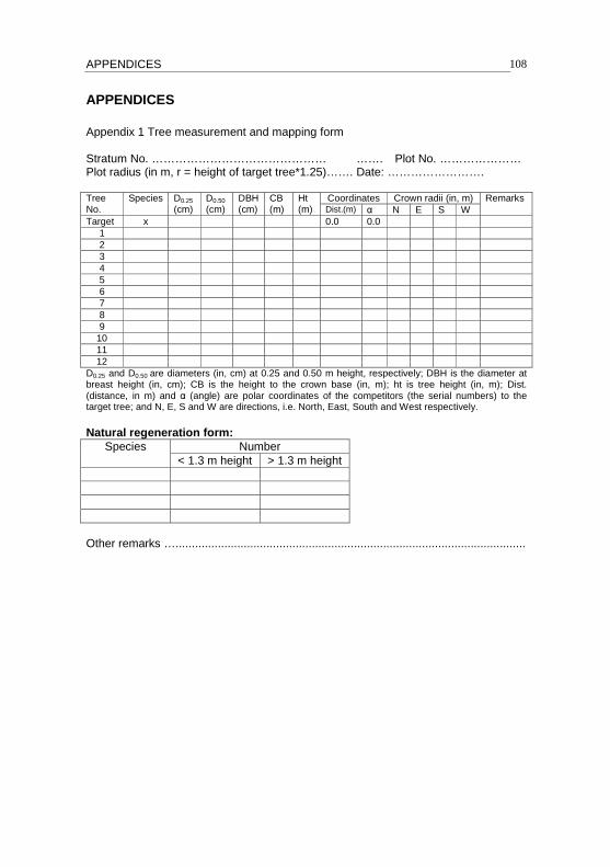
APPENDICES 108
APPENDICES
Appendix 1 Tree measurement and mapping form
Stratum No. ……………………………………… ……. Plot No. ………………… Plot radius (in m, r = height of target tree*1.25)……. Date: …………………….
Tree No.
Species D0.25
(cm) D0.50
(cm) DBH (cm)
CB (m)
Ht (m)
Coordinates Crown radii (in, m) Remarks Dist.(m) α N E S W
Target x 0.0 0.0
1
2
3
4
5
6
7
8
9
10
11
12
D0.25 and D0.50 are diameters (in, cm) at 0.25 and 0.50 m height, respectively; DBH is the diameter at breast height (in, cm); CB is the height to the crown base (in, m); ht is tree height (in, m); Dist.
(distance, in m) and α (angle) are polar coordinates of the competitors (the serial numbers) to the target tree; and N, E, S and W are directions, i.e. North, East, South and West respectively.
Natural regeneration form: Species Number
< 1.3 m height > 1.3 m height
Other remarks …............................................................................................................

APPENDICES 109
Appendix 2 Gum tapping and collection form
Stratum No. ……. ………………………… Plot No. ………………
Tapping date: □ 1st October □ 15th October□ 1st November
Target tree
Tapping tool
DBH (cm)
Height (m)
Crown base
Crown radii (m) Gum quantity (g) per collection
N E S W 1st 2
nd 3
rd 4
th 5
th 6
th 7
th
1
2
3
4
5
6
7
8
9
10
11
12
13
14
15
16
17
18
19
20
21
22
23
24
25
26
27
28
29
Remarks: …………………………………………………………………………………………………. ………………………………………………………………………………………………….………………………………………………………………………………………………….………………………………………………………………………………………………….………………………………………………………………………………………………….
………………………………………………………………………………………………….………………………………………………………………………………………………….

APPENDICES 110
Appendix 3 Normality test of A. seyal tree dimensions Stratum Index Mean Median SD Min. Max. Skewness Shapiro-Wilk
Statistic P-value
DBH 12.2 12.9 3.8 5.1 36.9 1.12 0.945 0.000
Dense Height 7.2 7.0 1.2 4.5 11.5 0.22 0.988 0.000
DBH 13.4 13.8 4.5 5.8 34.1 0.71 0.967 0.000
Medium Height 7.6 7.5 1.3 4.0 12.0 0.09 0.989 0.000
DBH 12.2 12.9 4.0 5.1 33.9 0.87 0.958 0.000
Slight Height 6.7 6.7 1.3 2.3 10.0 -0.02 0.989 0.000
Number of observations per stratum (dense = 1781; medium = 1235; slight = 783); SD = standard deviation
Appendix 4 Results of regression tree analysis for predicting gum talha yield
Node number Variable Split criterion N Deviance Gum yield (g)
1 Root node 482 751000 15.35
2 DBH < 23.95 cm 469 574200 13.53
4* Tool Untapped 105 29090 5.87
5 Tool Makmak, sonki 364 537200 15.74
10* Date 15th Oct, 1
st Nov 250 295800 12.61
11 Date 1st Oct 114 233600 22.59
22* CI < 3.915 109 158400 20.80
23* CI > 3.915 5 67210 61.69
3 DBH > 23.95 cm 13 119000 81.10
6* CI < 0.125 5 1330 11.40
7* CI > 0.125 8 78200 124.70
*. Denotes for terminal node; N = number of observations per split; nodes´ number are ordered
according to the regression tree model; CI = Hegyi_2 competition index
Appendix 5 Scheffe test (Post-hoc-test) after ANOVA for gum talha yield derived from natural A. seyal using different tapping tools in the Umfakarin Forest, South Kordofan, Sudan
Stratum Tool (I) Tool (J) Mean
Difference (I-J) Std. Error Sig.
95% Confidence Interval
Lower Bound Upper Bound
Dense Makmak
Sonky
Sonky 9.480 6.238 0.318 -5.943 24.903
Untapped 12.798 6.337 0.134 -2.870 28.466
Untapped 3.318 6.476 0.877 -12.694 19.330
Medium Makmak
Sonky
Sonky -10.100 5.613 0.201 -23.975 3.775
Untapped 5.758 7.940 0.769 -13.871 25.386
Untapped 15.858 8.139 0.153 -4.262 35.977
Slight Makmak
Untapped
Sonky .023 8.615 1.000 -21.270 21.316
Untapped 18.939 9.870 0.162 -5.455 43.333
Sonky -18.916 10.329 0.190 -44.445 6.613
Results are based on observed means.
The error term is Mean Square (Error) = 2337.915

APPENDICES 111
Appendix 6 GLM results: tests of between-subjects effects
Stratum Source SS DF MS F-value Sig. η²
Corrected Model 11680.673 10 1168.067 1.107 0.361 0.070 Intercept 470.807 1 470.807 0.446 0.505 0.003 BHD 2322.279 1 2322.279 2.201 0.140 0.015 CI 715.687 1 715.687 0.678 0.412 0.005 Dense Tool 4413.710 2 2206.855 2.091 0.127 0.028 Date 1782.141 2 891.071 0.844 0.432 0.011 Tool*Date 2898.767 4 724.692 0.687 0.602 0.018
Error 155132.502 147 1055.323 Total 189780.795 158 Corrected Total 166813.175 157 Corrected Model 60091.638 9 6676.849 7.293 0.000 0.304
Intercept 8558.918 1 8558.918 9.349 0.003 0.059 BHD 21085.447 1 21085.447 23.032 0.000 0.133 CI 2618.599 1 2618.599 2.860 0.093 0.019 Medium Tool 7383.671 2 3691.836 4.033 0.020 0.051 Date 22363.719 2 11181.859 12.214 0.000 0.140 Tool*Date 19305.564 3 6435.188 7.029 0.000 0.123 Error 137325.695 150 915.505 Total 225481.077 160
Corrected Total 197417.333 159 Corrected Model 33695.824 10 3369.582 1.489 0.148 0.089 Intercept 5975.268 1 5975.268 2.641 0.106 0.017 BHD 14864.197 1 14864.197 6.570 0.011 0.041
CI 10492.793 1 10492.793 4.638 0.033 0.029 Slight Tool 12009.690 2 6004.845 2.654 0.074 0.034 Date 5093.358 2 2546.679 1.126 0.327 0.015 Tool*Date 3166.788 4 791.697 0.350 0.844 0.009
Error 346145.902 153 2262.392 Total 449283.545 164 Corrected Total 379841.726 163
Dependent variable: gum talha yield (g) Dense: R² = 0.070 (Adjusted R Squared = 0.007)
Medium: R² = 0.304 (Adjusted R Squared = 0.263) Slight: R² = 0.089 (Adjusted R Squared = 0.029) CI = Hegyi_2 competition index; η² = Partial Eta squared; SS = sum of squares; MS = mean square; DF = degrees of freedom.
